Nutation in the Spinning SPHERES Spacecraft and Fluid

Slosh

Caley A. Burke, David W. Miller

June 2010 SSL # 7-10

2

3

Nutation in the Spinning SPHERES Spacecraft and Fluid Slosh

Caley A. Burke, David W. Miller

June 2010 SSL # 7-10 This work is based on the unaltered text of the thesis by Caley Ann Burke submitted to the Department of Aeronautics and Astronautics in partial fulfillment of the requirements for the degree of Masters of Science at the Massachusetts Institute of Technology.

4

5

Nutation in the Spinning SPHERES Spacecraft and Fluid Slosh

by

Caley Ann Burke

Submitted to the Department of Aeronautics and Astronautics on May 21, 2010 in partial fulfillment of the requirements for the degree of

Masters of Science in Aeronautics and Astronautics

Abstract

Spacecraft today are often spin-stabilized during a portion their launch or mission. Though the basics of spin stabilization are well understood, there remains uncertainty in predicting the likelihood of rapid nutation growth due to onboard liquids. Solely analytical methods of prediction are mainly unsuccessful and physical tests to gather slosh data have only been done for a few specific spacecraft. Data from past spacecraft is subject to a number complex physical factors and anomalies during the launch or mission.

This study verifies a ground based method to test fluid tanks horizontally and obtain the first fundamental frequency of the tank. Horizontal tanks have the gravitational acceleration vector applied in the same direction as the acceleration experienced by an offset tank on a spinning spacecraft.

The study also performs tests on the Synchronized Position-Hold, Engage, Reorient Experimental Satellites (SPHERES) satellites to characterize their nutation. In the tests, the satellite is spun about a single axis and then allowed to drift. Each principal axis is tested by at least one test. Two configurations of the satellite are tested: the satellite by itself and the satellite with an additional rigid mass attached to alter the inertia matrix of the system.

These two efforts can be combined in the future to perform spinning slosh testing on the SPHERES satellites, with knowledge of the frequency of the fluid tanks. The potential for the SPHERES Testbed to add to the generic fluid slosh data is due to it having a relatively simple spacecraft system capable of both software and hardware modifications and being located in the visually observable microgravity environment of the International Space Station (ISS).

Thesis Supervisor: David W. Miller

Title: Professor of Aeronautics and Astronautics

6

7

Acknowledgements

NASA - Kennedy Space Center (KSC) and the NASA Launch Services Program for providing the funding for this research via the Kennedy Graduate Fellowship Program Dr. David Miller for guidance throughout this study The SPHERES team for working with me to perform the research on the Testbed

8

9

Contents

List of Tables .......................................................................................................................... 13

List of Figures ......................................................................................................................... 15

Acronyms ................................................................................................................................ 19

Mathematical Variables ........................................................................................................ 20

Chapter 1 Introduction ................................................................................................... 23

1.1 Motivation ............................................................................................................. 23

1.2 Literature Review ................................................................................................. 24

1.3 SPHERES Testbed ................................................................................................ 25

1.4 Approach ............................................................................................................... 27

Chapter 2 Building a Model of the Problem (generic) ............................................... 29

2.1 Euler Equations of Motion .................................................................................. 29

2.2 Nutation Prediction ............................................................................................. 31

2.2.1 Nutation Definition ...................................................................................... 32

2.2.2 Excitation of Nutation .................................................................................. 34

2.2.3 Slosh ................................................................................................................ 35

2.2.4 Coupled Slosh and Nutation ....................................................................... 37

2.3 Nutation Determination Problem ...................................................................... 40

Chapter 3 Physical Environments of the Experiments .............................................. 41

3.1 Environment of the Horizontal Fluid Slosh Ground Tests ............................ 41

3.2 Geometry of a SPHERES satellite ...................................................................... 42

10

3.3 Inertia Models ....................................................................................................... 44

3.3.1 SPHERES Satellite ......................................................................................... 45

3.3.2 SPHERES satellite with additional rigid mass ......................................... 47

3.3.3 SPHERES Satellite with additional fluid mass ......................................... 49

3.3.3.1 Availability of Tanks for Additional Fluid Mass .................................. 50

3.4 Disturbance Torques ............................................................................................ 51

3.4.1 Atmospheric Drag ........................................................................................ 51

3.4.2 Gravity ............................................................................................................ 53

3.5 Design of Experiment .......................................................................................... 54

3.5.1 Horizontal Fluid Slosh Ground Tests ........................................................ 54

3.5.2 SPHERES Nutation in Microgravity .......................................................... 59

Chapter 4 Experimental Data ........................................................................................ 62

4.1 Horizontal Slosh Ground Tests .......................................................................... 62

4.2 SPHERES Nutation in Microgravity ISS Tests - Execution and Results ...... 65

4.2.1 Minor Axis Spin ............................................................................................ 67

4.2.2 Intermediate Axis Spin ................................................................................ 71

4.2.3 Major Axis Spin ............................................................................................. 72

4.2.4 Major Axis Spin of the SPHERE + Battery Pack Configuration ............. 74

4.2.4.1 Detecting Rotation Rate by Video ........................................................... 77

4.2.4.2 Open Loop Thrust Anomaly .................................................................... 78

4.2.5 Modifications of the Tests............................................................................ 81

4.2.5.1 Adding the Position Holds ...................................................................... 81

4.2.5.2 Removing stopping maneuver ................................................................ 83

4.2.5.3 Reducing time of IMU .............................................................................. 84

11

Chapter 5 Model Correlation ........................................................................................ 85

5.1 Horizontal Fluid Slosh Ground Tests ............................................................... 85

5.1.1 Frequency Modes .......................................................................................... 85

5.1.1.1 Previous Experimental Study .................................................................. 85

5.1.1.2 Correlation of Experiments ...................................................................... 86

5.1.2 The Effect of Fill Fraction on Slosh Power ................................................ 88

5.1.3 Applicability .................................................................................................. 89

5.1.4 Angular Momentum Conservation and the Drag Effect ........................ 90

5.2 Inertia Ratio Determination of Ground Based Test Model ............................ 92

5.3 Nutation Frequency of ISS Tests ........................................................................ 93

5.4 Nutation Time Constant Calculation ................................................................ 97

5.5 Open Loop Thrust ................................................................................................ 99

Chapter 6 Conclusions ................................................................................................. 101

6.1 Thesis Summary ................................................................................................. 101

6.2 Contributions ...................................................................................................... 102

6.3 Future Work ........................................................................................................ 102

Bibliography ............................................................................................................................. 105

12

13

List of Tables

Table 3.1 Thruster Geometry (in body coordinate frame) [8] .............................................. 43

Table 3.2 Inertia Models of the SN1 SPHERES (wrt the geometric center [GC]) [16] ...... 46

Table 3.3 Center of Mass (CM) Models of the SN1 SPHERES (wrt the GC) [16] .............. 46

Table 3.4 Inertia Effects on SN1 SPHERES satellite System due to the Addition of a

Battery Pack .......................................................................................................................... 48

Table 3.5 Container Dimensions .............................................................................................. 58

Table 4.1 ISS Nutation Test Matrix .......................................................................................... 66

Table 4.2 Minor Axis Spin Maneuvers .................................................................................... 68

Table 5.1 Inertia Ratios of the SPHERES satellites based on the Ground Measured

Inertia Values (Dry) [16] ...................................................................................................... 92

Table 5.2 Nutation Frequency of Each Test ............................................................................ 93

Table 5.3 ISS Measured Inertia Values .................................................................................... 97

Table 5.4 Various Calculations of Rotation Rate Increase .................................................. 100

14

15

List of Figures

Figure 1.1 SPHERES Satellite (with battery pack attached to left hand side) on the ISS [9]

................................................................................................................................................. 26

Figure 2.1(a) Nutation Motion (z is a geometric axis) (b) Nutation Angle [11] [6] ......... 32

Figure 2.2 Motion of the Nutating Spacecraft. ....................................................................... 33

Figure 2.3 Basic object with unequal Moments of Inertia, d < h < w and 321 III << ..... 33

Figure 2.4 Southwest Research Institute (SwRI) Spinning Slosh Test Rig (developed with

NASA) [14] ............................................................................................................................ 39

Figure 3.1 SPHERES Satellite with Body Axes and Thrusters 1/2 Identified [15] ........... 42

Figure 3.2 SPHERES Thruster Geometry [8] .......................................................................... 43

Figure 3.3 SPHERES Satellite with battery attached via Velcro –X face [17] .................... 48

Figure 3.4 SPHERES Satellite with No-Rinse Shampoo Bottles Attached ......................... 50

Figure 3.5 No Rinse Shampoo Bottle ....................................................................................... 51

Figure 3.6 SPHERES Spin Profiles (a) +Z spin (b) +Y spin (+X spin has the same profile)

(c) +Y spin with battery mass attached [20] ..................................................................... 53

Figure 3.7 MESSENGER Propellant Tank Configuration [22] ............................................ 55

Figure 3.8 Examples of cylinders oriented with the acceleration force .............................. 56

Figure 3.9 1-g Slosh Testing Set-up ......................................................................................... 57

Figure 4.1 Amplified Load Cell Data from a Container B 40% Fill Fraction ..................... 63

Figure 4.2 Power Spectral Density from a Container B 40% Fill Fraction Run ................. 65

16

Figure 4.3 Experimental First Longitudinal Modes for Containers A and B by Fill

Fraction .................................................................................................................................. 65

Figure 4.4 Body Axis Rotation Rates for Test 1: Minor Axis Spin (+Z) Test ..................... 68

Figure 4.5 Test 1 Position Location within the ISS Test Volume ......................................... 70

Figure 4.6 Test 1 IMU 1000Hz data (a) Accelerometers (b) Gyroscopes ............................ 70

Figure 4.7 Test 2 Body Axis Rotation Rates ............................................................................ 71

Figure 4.8 Test 3 Body Axis Rotation Rates ............................................................................ 73

Figure 4.9 Test 4 Body Axis Rotation Rates ............................................................................ 74

Figure 4.10 Test 5 Body Axis Rotation Rates .......................................................................... 75

Figure 4.11 Test 6 Body Axis Rotation Rates .......................................................................... 76

Figure 4.12 Test 6 Power Spectral Density of the Body Axis Rotation Rates .................... 78

Figure 4.13 Test 6 Thruster Commands .................................................................................. 80

Figure 4.14 Test 6 Disrupted IMU Data .................................................................................. 80

Figure 4.15 Test 4 Position and Velocity Data ....................................................................... 82

Figure 4.16 Test 3 Position and Velocity Data ....................................................................... 83

Figure 5.1 Experimental 1st Longitudinal Modes .................................................................. 87

Figure 5.2 Liquid Fill Fraction vs. Power Density of the 1st Longitudinal Mode ............. 88

Figure 5.3 The range of possible Inertia ratios for SN3 ........................................................ 94

Figure 5.4 Inertia Possible for SN1 .......................................................................................... 95

Figure 5.5 Angular Momentum Magnitude of the Test 2 for both the Ground and ISS

Measured Inertia Values ..................................................................................................... 96

17

Figure 5.6 Nutation Angle of (a) Test 3: Major Axis Spin (+X) Test (b) Test 5: Major Axis

Spin of the SPHERES + Battery Pack (+Y) Test: Rotation Rate 1.25 rad/s (c) Test 6:

Rotation Rate 6.28 rad/s ..................................................................................................... 98

18

19

Nomenclature

Acronyms

3DOF Three Degrees of Freedom 6DOF Six Degrees of Freedom CAD Computer-Aided Design CM Center of Mass CO2 Carbon Dioxide GC Geometric Center IMU Inertial Measurement Unit ISS International Space Station KSC Kennedy Space Center LOS Loss of Signal LV Launch Vehicle MAMS Microgravity Acceleration Measurement System

MESSENGER MErcury Surface, Space ENvironment, GEochemistry, and Ranging

MIT Massachusetts Institute of Technology MOI Moment of Inertia NASA National Aeronautics and Space Administration NTC Nutation Time Constant PMDs Propellant Management Devices PSD Power Spectral Density S/C Spacecraft SN SPHERES Number

SPHERES Synchronized Position-Hold, Engage, Reorient Experimental Satellites

SSL Space Systems Laboratory SwRI Southwest Research Institute TS Test Session

20

Mathematical Variables

1-g sea level gravity a acceleration A surface area Bo Bond number Cd coefficient of drag cm centimeter d depth E rotational kinetic energy F force f frequency Fd drag force g gravitational acceleration h height h height of liquid within the container Hz Hertz (1/s) I inertia i imaginary number (square root of 1) km kilometer L angular momentum vector L characteristic length scale l bottle length M force moment m meters mL milliliter N length of signal in time n nth parameter of that variable P principal axis psi pressure per square inch R radius of the cylinder

R distance of from the center of mass of a system to the center of mass of the fluid container

rad radians s seconds t time v velocity w width x signal of length N z nutation motion γn nth fluid frequency parameter

21

θ nutation angle λ nutation frequency ρ density σ surface tension of the interface σ sigma (distribution) τ nutation time constant (NTC) τ torque ω angular acceleration

angular velocity ω instantaneous rotation axis Ω rotation rate ω angular frequency ω1 first longitudinal natural frequency ωN Nth root of 1

22

23

Chapter 1

Introduction

This chapter contains the motivation of the work achieved in this thesis. It reviews

the literature for previous work performed. It summarizes the SPHERES Testbed, on

which some of the experiments in this thesis were executed. It concludes with the

approach of the study of nutation of spinning spacecraft and fluid slosh.

1.1 Motivation

Propellant fluid slosh in spacecraft can couple into the dynamics of the vehicle leading

to performance degradation in the propulsion and attitude stabilization sub-systems.

Spacecraft are frequently rotated for several reasons: to provide gyroscopic stability;

and to allow sensors or other hardware on the spacecraft to rotate. The rotation for

stability often required on spacecraft with solid propellant upper stages. The rotation

for sensors/hardware may be either for thermal reasons, for field of view purpose, or

other reasons specified by the scientific mission. Spacecraft tanks are often offset from

24

this spin axis so that the rotation induces a local acceleration that forces the fluid into

one side of the tank. This acceleration also provides an effective “stiffness” to the

fluid’s motion which, when coupled with the fluid’s inertia, results in slosh. This

oscillatory fluid motion then couples with the motion of the vehicle.

Understanding the dynamics of this fluid slosh is essential to the design of

mitigation techniques such as attitude control, fluid baffles, etc. Of particular interest

are conditions leading to resonance between the nutation motion and liquid modes,

which can result in rapid nutation growth. Rapid growth nutation can lead to a loss of

control of the spacecraft; a state where either the control system is either unable regain

control of spacecraft attitude or the control system has used most to all of its system’s

fluids overcoming the nutation, leaving minimal or no fluids available to perform the

mission. Tanks with cylindrical sections have been shown particularly susceptible to

this.

1.2 Literature Review

Purely analytical methods of predicting the effect of fluid slosh in microgravity have

had very limited success at this point. Capturing this understanding through the use of

dynamic models requires test data in order to accurately calibrate the models and

ensure that all of the important physics involved are properly captured. Since rotation

rates can differ, and these spacecraft are operating in the microgravity of space, it is

important to obtain test data at different acceleration levels. However, some of these

25

acceleration levels are less than 1-g and therefore difficult to create the reduced gravity

environment for long durations in a terrestrial laboratory.

There has been significant fluid slosh work performed today. Much of the work

takes place on the ground. [1] There is also extensive knowledge of how to analytically

predict the slosh of spheres and vertical cylinders. However, cylinders with the

acceleration applied horizontally are significantly more difficult to model and require

testing, once the tank changes beyond being a simple cylinder filled halfway. [2] [3] [4]

[5]

In spacecraft where rapid nutation growth is of high concern, physical modeling of

the tanks or spacecraft is often conducted. However, due to constraints, these tests are

often conducted either in the 1-g or simulated microgravity via a drop tower on the

miniature scale (capable of only ~2-3 seconds data per run). Additionally, the tests are

conducted for highly complex spacecraft that using a variety of tanks, system

configurations, and going to a variety of locations throughout the solar system. The

technical community is lacking global, non-mission specific data regarding fluid slosh

in microgravity. [6]

1.3 SPHERES Testbed

The Synchronized Position-Hold, Engage, Reorient Experimental Satellites

(SPHERES) Testbed was developed and is maintained by the Space Systems Laboratory

(SSL) at Massachusetts Institute of Technology (MIT). The testbed consists of six degrees

26

of freedom (6DOF) microsatellites capable of communicating with each other and the

computer. [7] [8]

The satellites are each approximately 4 kg and have a diameter of 20 cm (about the

size of a basketball).

Figure 1.1 SPHERES Satellite (with battery pack attached to left hand side) on the ISS [9]

At the time of the testing described within this paper, there were two sets of three

SPHERES satellites, located in two places: the SSL and the U.S. Laboratory of the

International Space Station (ISS). The SPHERES Testbed in the SSL is operated with

three degrees of freedom (3DOF) in a 1-g environment. The SPHERES Testbed on the

ISS is operated at a 6DOF in a microgravity environment.

27

Testing on the ISS is performed as a voluntary science, which occurs as allowed by

astronauts’ schedules. Multiple tests are grouped together and performed on the same

day to form a Test Session (TS).

1.4 Approach

This thesis focuses on the nutation of spinning spacecraft in microgravity with fluid

slosh. The test data analyzed divides into two sections: horizontal fluid slosh tests

performed in 1-g and nutation testing of the SPHERES satellites in microgravity. The

fluid slosh microgravity data gathered previously has been on functional spacecraft.

This study intends to use the SPHERES Testbed, to gather data in microgravity for a

relatively simple spacecraft system and be able to perform maneuvers specifically

designed with slosh in mind. The system is visibly observable via video cameras and in

person (an astronaut) and is able to be reset, both software wise and physically.

The approach to the experiments discussed within this thesis is as follows:

1. Horizontal fluid slosh experiments performed on the ground

• Develop method of determining the fundamental frequency of a

container via a test in the lab in 1-g

• Perform the method on containers with known fundamental

frequencies

• Multiple containers

• Multiple fill fractions of fluid (ratio of liquid in container to

volume of the container)

28

• Verify that the method achieved the expected fundamental frequencies

• Perform the method on the fluid tank(s) to be used in microgravity

testing [future work]

2. Nutation testing on the ISS

• Develop a test to be run on a SPHERES satellite that can measure the

nutation of a spinning spacecraft

• Perform the test on the ground

• Perform the test on the ISS for multiple configurations

• SPHERES satellite

• SPHERES satellite with a rigid mass attached

• Verify the test performed as expected

• Determine the mass properties of the SPHERES satellite

• Perform the test on the ISS [future work]

• SPHERES satellite with fluid tank

The thesis covers the nutation of spacecraft (Chapter 2), the setup of the tests

(Chapter 3), the performance and data of the tests (Chapter 4), and the analysis of the

test data (Chapter 5).

29

Chapter 2

Building a Model of the Problem (generic)

This chapter derives the equation for nutation frequency from the Euler Equations of

Motion, which can be applied generically to a rigid body rotating about a single

principal axis in microgravity. It then discusses how that nutation can be calculated,

why knowledge of nutation is important in a spacecraft system and how it can interact

with fluid slosh.

2.1 Euler Equations of Motion

The Euler Equations of Motion are three differential equations relating force

moments , angular velocities , and angular accelerations of a rotating rigid

body:

( )( )( ) 3211233

2133122

1322311

MIIIMIIIMIII

=−+=−+=−+

ωωωωωωωωω

2.1

The reference body fixed axes are assumed to be the principal axes of inertia. [10]

30

The Euler equations will be applied to the generic system with several assumptions:

1. The force moments exerted on the system are zero. 03,2,1 =M

2. The angular velocity for each axis consists of a set rotation rate (Ωi) and

incremental variance in that rotation rate (ωi). The angular acceleration is only

applied to the variance in the rotation rate.

111 ωω +Ω⇒ 2.2

3. The set rotations for the other two principal axes are zero. 03,2 =Ω

4. The set rotation rate for the first principal axis is to be significantly larger than

the variance in any three of the rotations. 3,2,11 ω>>Ω

5. The value of any variances in rotation values times another variance is zero

(i.e. remove nonlinearities from the system).

2.3

As the first two of these assumptions are applied to the Euler Equations, Equation

2.1 becomes:

( )( )( ) 0))((

0))((0))((

22111233

11333122

33222311

=+Ω+Ω−+=+Ω+Ω−+=+Ω+Ω−+

ωωωωωωωωω

IIIIIIIII

2.4

With the third assumption, Equation 2.4 becomes:

( )( )( ) 0)(

0)(0

2111233

1133122

322311

=+Ω−+=+Ω−+

=−+

ωωωωωω

ωωω

IIIIIIIII

2.5

With the final two assumptions, Equation 2.5 becomes:

31

( )( ) 0

00

211233

133122

11

=Ω−+=Ω−+

=

ωωωω

ω

IIIIII

I

2.6

By taking the Fourier transform of Equation 2.6, the equations are converted to state

space. The response is assumed to be oscillatory and to correspond to the frequency of

the variance in the rotation rates.

( )( ) 0

00

211233

133122

11

22

=Ω−+=Ω−+

=−=

=

ωωωω

ωλ

λ

IIsIIIsI

sIs

is

2.7

Equation 2.7 can be manipulated to

( )

( ) ( ) ( )

( )( ) 021132132

2

2

1313

3

121

3

21213

2

13132

=Ω−−+⇒

Ω−Ω−=

Ω−=

Ω−=

IIIIIIs

sIII

sIII

sIIIsIII

ωωω

ωω

2.8

By moving out of state space and solving for the variance frequency, Equation 2.8

becomes

( )( )32

13211 II

IIII −−Ω±=λ

2.9

This variance frequency is known as the nutation frequency .

2.2 Nutation Prediction

Nutation references in this study will be defined in terms of common spacecraft

usage. This differs from the classic mechanics description, which involves a prominent

gravitational field causing vertical wobble in a spin axis [11].

32

2.2.1 Nutation Definition

Nutation is rotational motion for which the instantaneous rotation axis is not aligned

with a principal axis. There are three vectors involved in nutation:

: the angular momentum vector. It is fixed in inertial space.

: the principal axis which is rotating about L. It is fixed to the spacecraft, due to

inertia properties.

ω: instantaneous rotation axis. It rotates about both inertial space and the

spacecraft.

(a) (b)

Figure 2.1(a) Nutation Motion (z is a geometric axis) (b) Nutation Angle [11] [6]

The angle between the principal axis and angular momentum vector is called the

nutation angle ; it measures the magnitude of nutation. Given the following

conditions, the nutation angle will ideally remain constant: the other two of the

principal moments of inertia are equal, the nutation angle is small, there are no external

forces/torques on the system, and there is no energy dissipation in the system. The

movement of ω follows the intersection of a space cone and body cone, as shown in

Figure 2.2.

33

(a) (b)

Figure 2.2 Motion of the Nutating Spacecraft.

The body cone rolls on the space cone for (a) 321 III <= (b) 321 III <= [11]

Once the secondary principal moments of inertia are no longer equal, cone cross-

sections become elliptical instead of circular and the nutation angle loses the possibility

of remaining constant.

Figure 2.3 Basic object with unequal Moments of Inertia, d < h < w and 321 III <<

For any spacecraft with its principal moments of inertia such that 321 III << , the

spacecraft may spin stably about either I3 (the major axis) or I1 (the minor axis). In either

case, small perturbations produce bounded deviations from the nominal state. In cases

34

where 21 II ≈ , major axis spin is commonly referred to as Frisbee spin. In cases where

23 II ≈ , minor axis spin is commonly referred to as pencil spin.

However, spin about I2 (the intermediate axis) is unstable and small perturbations

produce unbounded deviations from the nominal state. The nutation frequency is

always an imaginary value. The axis of rotation should not be the intermediate axis.

2.2.2 Excitation of Nutation

Torques can affect the nutation of the system. The type of torque and how it is

applied determines the effect.

External torques on the system come in two main forms: disturbance torques from

the environment (i.e. drag) and control torques from attitude control (i.e. gas jets). If the

torque is applied parallel/anti-parallel to the angular momentum vector, the magnitude

of the angular momentum will increase/decrease. A torque applied perpendicular to

the angular momentum vector will change the direction of the vector along with its

magnitude, which is called precession.

Internal torques cannot change the value of the angular momentum vector in inertial

space. However, they can affect angular momentum vector in relation to the spacecraft

frame. Possible causes of energy dissipation due to internal forces in spacecraft are the

system (damping by the structure), spacecraft components (including fluids), and

nutation damping hardware.

If internal torques cause energy dissipation, the rotational kinetic energy of the

spacecraft will decrease. Equation 2.10 shows how the rotational kinetic energy ( )E

35

relates to the spacecraft principal moments of inertia ( )I and those axes’ corresponding

angular velocity and momentum vector components ( )L in a rigid spacecraft [11].

( )

++=++=

3

23

2

22

1

212

33222

211 2

121

IL

IL

ILIIIEk ωωω

2.10

For a constant value of L, rotational kinetic energy decreases by transferring the

angular momentum to its component corresponding to the largest principal moment of

inertial (major principal axis). Once rotational kinetic energy is at its minimum, the

energy dissipation ceases and the angular momentum vector is aligned with the major

principal axis.

In cases where the intended axis of rotation is the major principal axis, this is known

as nutation damping and excess kinetic energy is removed from the system. In cases

where the intended axis of rotation is not the major principal axis, this could be

disastrous for the spacecraft.

Rapid nutation growth can lead to loss of control. This may cause the spacecraft to

use excess propellant to control the spacecraft, which shortens the life of the spacecraft.

It could also result in loss of the spacecraft or mission. The intent of spin stabilization is

usually to give gyroscopic stability. If an object spinning about a minor axis has any

flexibility, it will need to have nutation damping capabilities, either active or passive, on

board.

2.2.3 Slosh

The energy dissipation that this study will focus on is fluid slosh, specifically

propellant slosh. Propellant slosh “refers to free surface oscillations of a fluid in a

36

partially filled tank resulting from translational or angular acceleration of [the]

spacecraft.” [11] The acceleration could be caused by the control system, flexibility in

the spacecraft structure, or an environmental disturbance.

The oscillations are movement of the liquid propellant within the tank, caused by

the balance of inertia and surface tension forces. The Bond Number characterizes

the ratio between acceleration to surface tension forces, as seen in Equation 2.11. [12]

The surface tension forces are defined by the density of the fluid , surface tension of

the interface and the characteristic length scale . On a spinning spacecraft in

microgravity, the acceleration input is the centrifugal acceleration and not gravity, since

generally gR >>Ω2 (R is the distance from the spin axis to the free surface).

σρ 2aLBo =

2.11

For cases when 1<<Bo , surface tensions dominate and the fluid free surface climbs

the tank walls. As the Bond number decrease, so do the components of natural

frequency.

The following trends have high risk for significant slosh energy: large propellant

tanks (the fluid is a significant percentage of the total spacecraft [S/C] mass) and

intermediate fill fraction (i.e. ~60%) [13]. Each trend can independently create

significant slosh energy, but having both trends present is what really creates the high

risk situation. A tank filled 100% with fluid does not allow motion of the location of the

fluid within the tank and an empty tank has no fluid to impact force, which is why

these fill fractions are not high risk conditions for slosh.

37

Since standard tank walls generally provide minimal damping effects, propellant

management devices (PMD) are often placed within the tank to increase slosh damping.

Though this study will not be addressing PMDs, some examples are: baffles,

diaphragms, vanes.

2.2.4 Coupled Slosh and Nutation

By determining the Nutation Time Constant (NTC) early in the design, it can be

used to determine if the current control system will be able to keep nutation under

control or if additional PMDs or other changes are necessary. The accuracy of the NTC

is important, as it is required as an input to the stability analysis for spinning launch

vehicle upper stage or spacecraft flight.

The upper stages spin to provide gyroscopic stabilization during orbital transitions.

Due to geometric constraints imposed by the launch vehicle, this spin is about the

minimum moment of inertia. The flexibility in the spacecraft leads to energy

dissipation, which then lead to instability. Fluid slosh is a source of flexibility and

therefore is also a source of energy dissipations.

Coupled resonance occurs when the nutation frequency is at or near the liquid

modal frequency. There is rapid energy dissipation and nutation change. The liquid

modal frequency changes as the propellant is depleted, so all fill levels of the tank must

be considered for coupled resonance.

Since the frequencies of both nutation and the slosh are proportional to spin rate (as

discussed in relation to Equation 2.1 and later demonstrated in 5.1.1.2), coupled

38

resonance cannot be avoided in a system simply by altering the spin rate. However, it

may be less severe at lower spin rates.

The calculation of the nutation angle over time requires knowledge of τ, the

NTC of the spacecraft. Equation 2.12 assumes that the initial nutation angle )( 0θ is

small (no more than a few degrees).

τθθ te0= 2.12

The NTC can be either positive or negative, depending on if nutation is growing or

decaying (minor or major axis spin). When there is fluid on board or flexibility in the

S/C, the NTC is very difficult to calculate, especially in early S/C design. Simulations of

propellant slosh often utilize mechanical analogs, such as pendulums and rotors, to

replace full fluid modeling. Analytical methods of predicting liquid frequencies are

possible, but usually underestimate the effect on nutation growth rates. Analytical

methods of obtaining resonant NTC are often off by an order or two of magnitude. [6]

The most accurate determination comes from flight or test data. Prior to flight, the NTC

can be calculated through forced motion (spin table in Figure 2.4), drop tower (free-fall),

ballistic trajectory, and air-bearing tests.

39

Figure 2.4 Southwest Research Institute (SwRI) Spinning Slosh Test Rig (developed with NASA) [14]

Through testing, groups can be determined for off-axis fluid tanks with variances in

the height and diameter of tank, as slosh is not very sensitive to these factors. These

groups are classified by nondimensional constants, such as the length to diameter ratio

of a cylindrical tank. However, NTC is very sensitive to factors such as fill fraction,

inertia ratio, tank shape, internal hardware (i.e. PMDs), and the tank location within the

S/C and so these dimension/values must be constant within a group.

If the tank is off-set from the spin axis of the spacecraft, the slosh modes will most

likely be higher than the nutation frequency and not cause coupled resonance; any

surface modes resulting from slosh would be small. However, if the tank is in-line, there

is the possibility of coupled resonance between the two frequencies and therefore large

surface waves: nutation synchronous motion. This complex motion is a rapidly

40

increasing rotating dynamic imbalance, visible in the jump of nutation angle, and the

corresponding NTC in such cases is uncontrollable. [6]

2.3 Nutation Determination Problem

Nutation determination is an involved and expensive process, so it is generally not

performed without a specific need. Testing in microgravity and other methods of

nutation determination are usually only performed for spacecraft where there is a

concern about rapid nutation growth. These spacecraft are usually very complicated, so

the data obtained is difficult to apply to other systems.

This study observed nutation in a simple spacecraft system in microgravity. By

characterizing nutation without and without additional fluid masses, the effect of the

fluid masses can be determined. The data from the simplified system is then

transferable. This thesis contains data only for the nutation of the spacecraft system

without additional fluid masses.

41

Chapter 3

Physical Environments of the Experiments

This chapter describes the environments of the experiments performed and follows

with the design of the experiments: horizontal fluid slosh ground tests and SPHERES

Nutation in Microgravity. The location and assumptions of the ground tests performed

are stated. Then the properties of the SPHERES satellite are detailed; this includes

masses that will be added to the satellite system (solid mass and fluid tanks). The

disturbance torques encountered in the ISS by the satellite are discussed. Finally the

design of each experiment is outlined.

3.1 Environment of the Horizontal Fluid Slosh Ground Tests

The ground tests were performed in an MIT lab. Average sea level atmospheric

conditions and gravity acceleration are assumed.

42

3.2 Geometry of a SPHERES satellite

Figure 3.1 SPHERES Satellite with Body Axes and Thrusters 1/2 Identified [15]

Figure 3.1 is a Computer-Aided Design (CAD) rendering of a SPHERES satellite,

with the body axes labeled. Through the center of the satellite is a CO2 propellant tank,

which aligns with the Z-axis. The propellant tank aboard the SPHERES satellite contains

nominally 172 g of CO2 when the tank is “full”, which is when the liquid fill is 68% of

the capacity of the tank. The SPHERES satellite is powered by two battery packs, which

are accessed by two magnetic doors located behind the +Y and –Y faceplates.

43

Figure 3.2 SPHERES Thruster Geometry [8]

Having twelve thrusters allows the satellite to have six degrees of freedom

capability. Figure 3.2 shows the locations of each thruster on a two dimension map of a

SPHERES satellite. Table 3.1 shows the direction of thrust for each thruster.

Table 3.1 Thruster Geometry (in body coordinate frame) [8]

Thruster Thruster position [cm] Nominal force direction Nominal torque direction

x y z x y z x y z 0 -5.16 0 9.65 1 0 0 0 1 0 1 -5.16 0 -9.65 1 0 0 0 -1 0 2 9.65 -5.16 0 0 1 0 0 0 1 3 -9.65 -5.16 0 0 1 0 0 0 -1 4 0 9.65 -5.16 0 0 1 1 0 0 5 0 -9.65 -5.16 0 0 1 -1 0 0 6 5.16 0 9.65 -1 0 0 0 -1 0 7 5.16 0 -9.65 -1 0 0 0 1 0 8 9.65 5.16 0 0 -1 0 0 0 -1 9 -9.65 5.16 0 0 -1 0 0 0 1

10 0 9.65 5.16 0 0 -1 -1 0 0 11 0 -9.65 5.16 0 0 -1 1 0 0

44

The SPHERES satellites have an inertial sensor suite: three rate gyroscopes and three

accelerometers. They can record data at 1000 Hz and have respective ranges of ± 1.45

rad/s and ± 25.6 mg. The satellites also have a Position and Attitude Determination

System global metrology system, which uses a global reference frame of either the

laboratory or the ISS.

On the SPHERES satellites, the -X face has Velcro attach points, which can be used to

attach the satellites to one another. Though this is most often used in docking

experiments, the Velcro can also be used to attach two SPHERES satellites together or

attach a used battery pack to a SPHERES satellite to perform tests with altered inertia.

There is a used battery pack on the ISS that has Velcro applied in the corresponding

pattern as on the SPHERES satellite.

3.3 Inertia Models

As when modeling any physical system, knowledge of the specifics of the system is

an issue. The main source for the nutation of a SPHERES satellite is the inertia

properties. With the exception of the CO2 liquid inside the propellant tank, there is

minimal flexibility within the SPHERES satellite system. The SPHERES satellite system

was noted to experience fluid slosh within its propellant tank in [16]. However, the

effect of noise produced by the slosh on the online mass property estimation was

considered negligible in comparison to the gyro ringing and thruster variability. Since

the majority of the tests performed on the SPHERES Testbed concern algorithms that

employ state estimation, the negligible coupling of nutation with the fluid slosh on the

45

SPHERES satellite do not effect those tests and therefore has not been fully studied.

Also, the spin rates have been very slow in all previous tests, making the nutation

frequency negligible.

3.3.1 SPHERES Satellite

Prior to this study, there were three inertia models of the SPHERES satellites.

• Analysis Model – CAD

o This model was developed by Payload Systems, Inc. [15]

• Test Model – derived from Ground Based Measurements

o This model was developed by in MIT’s SSL at 1-g, using a test stand

built in the lab. [16]

o σ = 2*10-3 kg-m2

• Test Model – derived from KC-135 Microgravity Measurements

o A series of rotational and translational tests were performed in the KC-

135 reduced gravity airplane microgravity environment. [7]

o As the microgravity in this environment is only available in 10-15

second increments, these tests were severely limited in time.

The models are given in Table 3.2. The serial numbers of the SPHERES satellites are

given as SN# (i.e. SN1). This notation indicates the specific SPHERES satellite that the

inertia models given measured; the CAD model applies to all SPHERES satellites. Wet

indicates that the model includes the CO2 fluid in the propellant tank, at a fill fraction of

68% liquid by volume; dry indicates the model is without the fluid.

46

Table 3.2 Inertia Models of the SN1 SPHERES (wrt the geometric center [GC]) [16]

(kg m2)*10-2 CAD Model

Measured

Ground, Microgravity (plane) (Dry) (Wet) (Dry) (Wet) (Wet)

Ixx 2.19 2.3 2.45 2.57 2.84

Iyy 2.31 2.42 2.15 2.25 2.68

Izz 2.13 2.14 2.03 2.03 2.36

Ixy 0.01 0.01 - - -0.0084

Ixz -0.03 -0.03 - - 0.0014

Iyz 0 0 - - -0.029

A very notable difference in the inertia matrices is the designation of the major and

intermediate axes. Although the CAD model and two test derived models give the Z-

axis as the minor axis, the CAD model assigns the Y-axis as the major axis and the other

two models assign the X-axis as the major axis.

Table 3.3 Center of Mass (CM) Models of the SN1 SPHERES (wrt the GC) [16]

CM Offset from GC (mm)

CAD Model Ground Test

Model (Dry) (Wet) (Dry) (Wet)

X 0.49 0.48 0.37 0.82 Y -1.24 -1.19 -1.52 -0.99 Z 3.98 1.08 3.32 1.07

The center of mass (CM) is close to but not exactly at the geometric center and varies

with the models and any additional of mass to the system. However, for this system, the

CM is never more than 4mm off and has a minimal effect on the system nutation. The

measured ground model, found through hardware testing, lists individual values for

each SPHERES satellite and is the most recently developed midel.

Testing of the SPHERES satellites in microgravity on the ISS indicated the ground

based testing model to be the closest to truth and it is used as the starting value for the

47

inertia matrices. However, the ground based testing model has only two fluid

configurations of the SPHERES satellite: without fluid in the CO2 tank and with a CO2

tank at its maximum liquid fluid fill (68%). Therefore the variable CO2 component in

microgravity has to be added to the inertia matrix. The amount the moments of inertia

(MOIs) increase is dependent on the amount of fluid in the tank and the configuration

of the fluid within the tank. So the MOIs of the SPHEREs are constantly changing due

to propellant usage, the accelerations exerted on the tank and free surface interactions

of the fluid. When calculating the nutation, the particular configuration for that test

must be considered (i.e. the fill level and location of the fluid within the CO2 tank). At a

maximum, the moments of inertia (MOI) for the X- and Y-axes will increase by 4.5%

and the Z-axis by 0.2% due to the fluid mass.

3.3.2 SPHERES satellite with additional rigid mass

The addition of rigid mass(es) to the SPHERES satellite allows for observing the

effect of adding mass without introducing flexibility to the system. The rigid mass alters

the center of mass and the inertia matrix of the SPHERES satellite. As the inertia of a

system is changes, so does the nutation. However, since all mass added is solid, the

change in the nutation is due to only to the change inertia and not by adding energy

dissipation to the system. This requires the attachment of the mass to have only

minimal flexibility, so not to have energy dissipate through the attachment point.

The Velcro on the –X face provides a good connection between the objects, which the

astronaut has the option of reinforcing with Kapton tape.

48

Figure 3.3 SPHERES Satellite with battery attached via Velcro –X face [17]

The mass and dimensions of the battery pack are well known. The mass is assumed

to be evenly distributed, as there is minimal space between the batteries. Table 3.4

shows the resulting change in inertia of the SPHERES satellite system from adding a

battery pack. It gives the inertia matrix for the cases where the battery pack is centered

exactly over the -X face and where it is off by 1 cm each in the +Y and +Z directions,

possible due to human error.

Table 3.4 Inertia Effects on SN1 SPHERES satellite System due to the Addition of a Battery Pack

(kg m2) 10-2 No Additional Mass Battery Pack Attached to -X face

Centered 1cm offset in +Y and +Z

Ixx 2.450 2.455 2.459

Iyy 2.150 2.424 2.425

Izz 2.030 2.302 2.305

Ixy - 0.003 0.028

Ixz - -0.007 0.017

Iyz - 0.000 -0.002

An important note from the inertia change due to the battery pack is that the major

and intermediate axes are now within 4*10-4 kg-m2 (~2%) of each other and the one

sigma value for the model is 2*10-3 kg-m2. The built-in uncertainty means that it is

49

possible for the major and intermediate axes to actually be able to switch. The addition

of a rigid mass 5.5% of the mass of the SPHERES satellite has dramatically changed the

nutation properties of the system and which axes it can stably spin about. The effect on

the inertia ratios must be considered when adding any mass to the SPHERES satellite

system.

3.3.3 SPHERES Satellite with additional fluid mass

The addition of fluid mass to the SPHERES satellite system has all the same effects

of adding a rigid mass plus it introduces a new source of flexibility and energy

dissipation to the system.

Symmetry with respect to the spin axis is desirable so to keep the center of mass

close to the geometric center of the SPHERES satellite system. The longitudinal axis of

the cylindrical fluid containers is parallel to the spin axis. The setup in Figure 3.4 is for

spin about the +Y axis; the +Y face of the SPHERES satellite in the figure has the

SPHERES logo on it.

50

Figure 3.4 SPHERES Satellite with No-Rinse Shampoo Bottles Attached

to the +X and –X faces for +Y Spin

3.3.3.1 Availability of Tanks for Additional Fluid Mass

This study intends to test slosh in microgravity conditions by adding fluid tanks

already available on the ISS. This additional liquid mass within the fluid tank could be

added to the SPHERES satellite system to observe fluid slosh. This option is seriously

considered for several reasons.

The modeling of off-axis tanks in spinning spacecraft is better understood by the

community at this time than on-axis tanks. This would allow for better correlation of

the test results to the models developed. Also, there would be a level of control over the

amount of fluid and fill fraction of the additional liquid masses that does not exist for

the onboard CO2 tanks.

At the maximum propellant load, the fluid mass of the SPHERES satellite is never

greater than 4% of the system mass. Since tanks are only changed on a needed basis and

test order is predetermined for SPHERES test sessions, the mass of the CO2 at the start

of any test could vary between 26-172 g. The mass of the CO2 is best known soon after

51

installation. After that, thruster use is tracked, but thruster variability leads to

inaccuracy in the estimate of the remaining CO2.

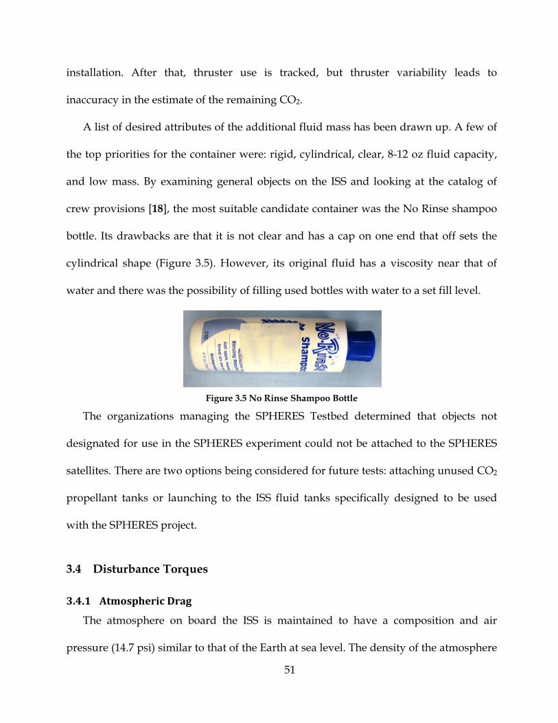
A list of desired attributes of the additional fluid mass has been drawn up. A few of

the top priorities for the container were: rigid, cylindrical, clear, 8-12 oz fluid capacity,

and low mass. By examining general objects on the ISS and looking at the catalog of

crew provisions [18], the most suitable candidate container was the No Rinse shampoo

bottle. Its drawbacks are that it is not clear and has a cap on one end that off sets the

cylindrical shape (Figure 3.5). However, its original fluid has a viscosity near that of

water and there was the possibility of filling used bottles with water to a set fill level.

Figure 3.5 No Rinse Shampoo Bottle

The organizations managing the SPHERES Testbed determined that objects not

designated for use in the SPHERES experiment could not be attached to the SPHERES

satellites. There are two options being considered for future tests: attaching unused CO2

propellant tanks or launching to the ISS fluid tanks specifically designed to be used

with the SPHERES project.

3.4 Disturbance Torques

3.4.1 Atmospheric Drag

The atmosphere on board the ISS is maintained to have a composition and air

pressure (14.7 psi) similar to that of the Earth at sea level. The density of the atmosphere

52

at 200 km is eight orders of magnitude smaller than the density of the air inside the ISS.

[11] So while spacecraft in low Earth orbit do have to account from atmospheric drag, it

is more often concerned with the lifetime of the mission and orbit maintenance.

However, when tests consider the physical system, atmospheric drag (3.1, [19]) is a

significant external force on the SPHERES satellite within the ISS and cannot be

considered negligible. This is particularly true when increasing the velocity of the

SPHERES satellite, since that causes an exponential increase in drag. The other factors

in drag force are the density of the fluid , surface area and coefficient of drag

.

3.1

In this study, the SPHERES satellite spins in along each of its three principal axes.

Additionally, it spins along its Y-axis with a configuration change that includes a

battery pack attached at the +X face. Though the coefficient of drag has not been

calculated for any of the cases, observation indicates that it would be lowest for the Z-

axis spin and highest for the Y-axis spin with battery attachment, with the DC for X-axis

and Y-axis spin just being a little smaller when without the battery pack attached. This

is illustrated in Figure 3.6 , which shows the obtrusions of the knob and tank in the +Y

and +X spin and the additional obtrusion of the battery pack when it is attached. The

system with the battery pack attached also has a higher surface area, as will any system

with additional mass attachments, which increases the drag force.

53

(a) (b) (c)

Figure 3.6 SPHERES Spin Profiles (a) +Z spin (b) +Y spin (+X spin has the same profile) (c) +Y spin with battery mass attached [20]

As discussed in 2.2.2, atmospheric drag is an external force and will change the

angular momentum vector of the spacecraft in inertial space.

3.4.2 Gravity

The ISS is in a free fall state and therefore objects within it results in microgravity

levels of acceleration. The quasi-steady acceleration measured by the Microgravity

Acceleration Measurement System (MAMS) indicates that the magnitude of the mean

acceleration experienced by that instrument aboard the ISS was less than 0.3 gµ in all

directions, and never more than 4 gµ ; this acceleration is due to the center of gravity

offset from the ISS to the MAMS and vibrations within the ISS. The MAMS published

data for two out of the three days in which SPHERES testing occurred for this study; the

acceleration values given apply directly to those days and are assumed to be true for the

third day. [21]

For a tank radius of 1 cm, as long as the SPHERES satellite was spinning at more

than 0.0626 rad/s, the centrifugal acceleration experienced by the fluid would be

greater than the free fall acceleration. Since the rotation rates in this study are more than

54

an order of magnitude greater than that rate, the effect of gravity is not factored into the

physical system.

3.5 Design of Experiment

The experiment plan has multiple phases:

• Observe fluid slosh in horizontal cylinders at 1-g

• Characterize nutation of the SPHERES satellite spinning in microgravity

• Characterize nutation of the SPHERES satellite spinning in microgravity with a

rigid mass attached

• Characterize nutation of the SPHERES satellite spinning in microgravity with

fluid tanks attached

This study executed the first three phases and discusses the results. Implementation

of the final phase is discussed in the future work section.

3.5.1 Horizontal Fluid Slosh Ground Tests

The end phase of the experiment plan involves observing the fluid slosh in tanks in

microgravity. To better understand the fluid slosh in the tanks, this study observed

fluid slosh in horizontal cylinders in 1-g.

The configuration of horizontal cylinders was chosen for a couple of reasons. Fluid

slosh in spheres is currently well understood and there are many models already

available, so exploration of this shape was limited in possible contributions. Spacecraft

propellant tanks are frequently cylinders with hemi-spherical ends. The acceleration

experienced due to centrifugal force in off-axis tanks on spacecraft is in the same

55

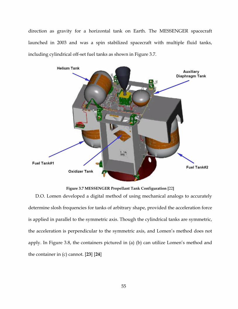
direction as gravity for a horizontal tank on Earth. The MESSENGER spacecraft

launched in 2003 and was a spin stabilized spacecraft with multiple fluid tanks,

including cylindrical off-set fuel tanks as shown in Figure 3.7.

Figure 3.7 MESSENGER Propellant Tank Configuration [22]

D.O. Lomen developed a digital method of using mechanical analogs to accurately

determine slosh frequencies for tanks of arbitrary shape, provided the acceleration force

is applied in parallel to the symmetric axis. Though the cylindrical tanks are symmetric,

the acceleration is perpendicular to the symmetric axis, and Lomen’s method does not

apply. In Figure 3.8, the containers pictured in (a) (b) can utilize Lomen’s method and

the container in (c) cannot. [23] [24]

56

(a) (b) (c)

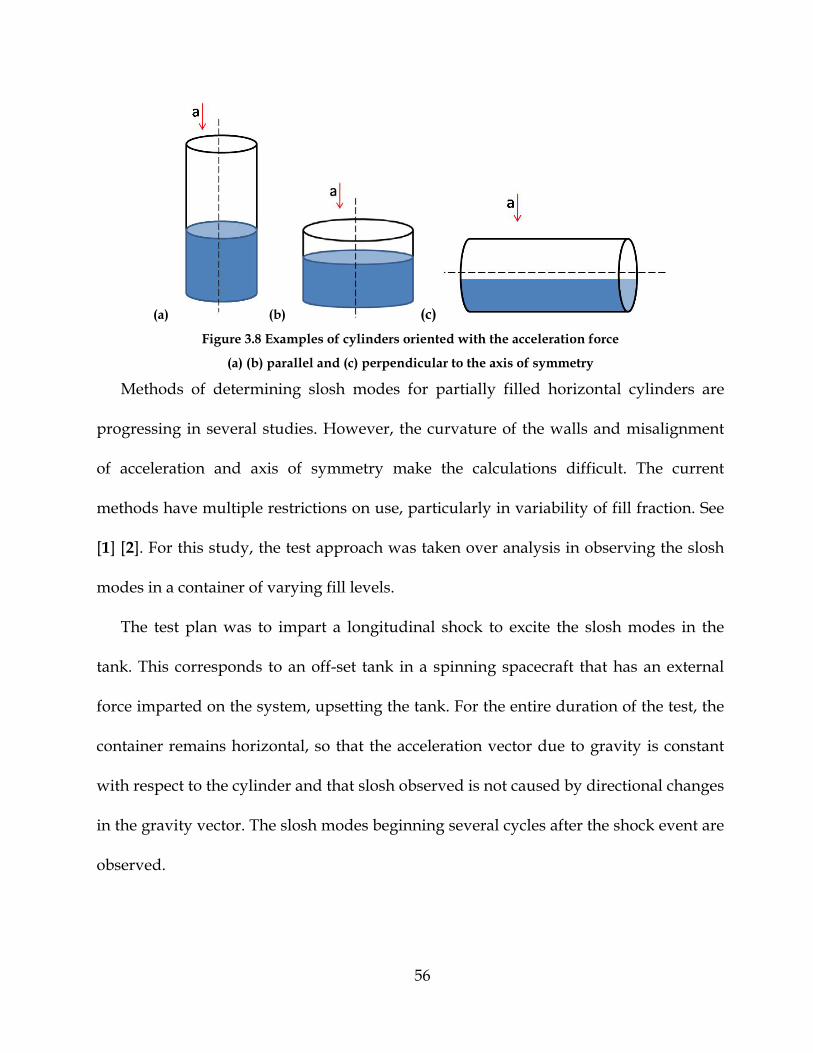
Figure 3.8 Examples of cylinders oriented with the acceleration force

(a) (b) parallel and (c) perpendicular to the axis of symmetry

Methods of determining slosh modes for partially filled horizontal cylinders are

progressing in several studies. However, the curvature of the walls and misalignment

of acceleration and axis of symmetry make the calculations difficult. The current

methods have multiple restrictions on use, particularly in variability of fill fraction. See

[1] [2]. For this study, the test approach was taken over analysis in observing the slosh

modes in a container of varying fill levels.

The test plan was to impart a longitudinal shock to excite the slosh modes in the

tank. This corresponds to an off-set tank in a spinning spacecraft that has an external

force imparted on the system, upsetting the tank. For the entire duration of the test, the

container remains horizontal, so that the acceleration vector due to gravity is constant

with respect to the cylinder and that slosh observed is not caused by directional changes

in the gravity vector. The slosh modes beginning several cycles after the shock event are

observed.

57

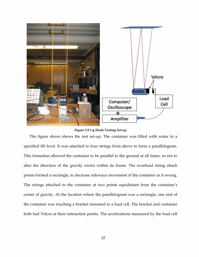
Figure 3.9 1-g Slosh Testing Set-up

The figure above shows the test set-up. The container was filled with water to a

specified fill level. It was attached to four strings from above to form a parallelogram.

This formation allowed the container to be parallel to the ground at all times, so not to

alter the direction of the gravity vector within its frame. The overhead string attach

points formed a rectangle, to decrease sideways movement of the container as it swung.

The strings attached to the container at two points equidistant from the container’s

center of gravity. At the location where the parallelogram was a rectangle, one end of

the container was touching a bracket mounted to a load cell. The bracket and container

both had Velcro at their interaction points. The accelerations measured by the load cell

58

are amplified and recorded by passing through an amplifier to an oscilloscope to a

computer with LabView.

The test was performed by drawing back the container a prescribed distance from

the bracket/load cell configuration, ensuring it is level with the ground. Once the fluid

had settled, the container was released and struck the bracket. The container and

bracket fastened to one another. The fluid within the container was excited by the shock

event. It then sloshed to its natural frequencies, which were observed via the

accelerations recorded throughout the test. The test was performed between 2-8 times

each for fill fractions ranging from 10% to 90% for Container A; the drawback distance

was kept approximately the same, but was not measured. The test was performed three

times each for three different draw back distances (5, 10, 15 cm) for fill fractions ranging

from 10% to 60% for Container B.

Possible sources of error in the test included the flexibility the Velcro connection at

the attach point, the difficulty in keeping the container level with ground and verifying

this, and any angle between the end of the container and the bracket, caused by an

indirect initial connection.

The results given for this study are for two cylindrical containers with smooth walls

and some imperfections at the end caps. The fluid used was water.

Table 3.5 Container Dimensions

Container Diameter Length Fluid Capacity

cm cm mL A 5 17 550 B 6.5 15 504

59

The tests performed are preliminary and demonstrate the method for obtaining 1-g

slosh modes for a horizontal cylindrical container. The tests also show trends in slosh

based on fill factor. Once go ahead is given to test attach fluid tanks to the SPHERES

satellite on the ISS and the fluid container is definite, these 1-g tests should be

performed again with that container and containing the fluid to be in it on the ISS.

3.5.2 SPHERES Nutation in Microgravity

In order to characterize the nutation of the SPHERES satellite, with and without a

rigid mass attached, four separate test configurations were performed over three test

sessions:

• SPHERES satellite spinning about the X-axis

• SPHERES satellite spinning about the Y-axis

• SPHERES satellite spinning about the Z-axis

• SPHERES satellite with a rigid mass attached spinning about the Y-axis

The intention of the tests was to observe a growing or decaying nutation angle

(depending on spin axis), in order to better understand nutation of the SPHERES

satellite system. Then, when additional fluid masses are later added, the nutation due to

the fluid masses only can be extracted and therefore determine the impact of the fluid

masses on the dynamics of the system as a whole. Also, the rigid body tests were

intended verify the accuracy of the inertia ratios with the nutation frequency.

The design of each test followed the following general procedure:

1. Calibrate the estimator

2. Stop in the middle of the test volume

60

3. Spin up to a set rotation rate about the designated spin axis

4. Turn off all control for a short period of time (i.e. drift)

5. Torque the SPHERES satellite about the X-axis via a short thruster pair firing

6. Turn off all control for a long period of time (i.e. drift)

7. Bring the vehicle to a physical stop

The first two steps were the set-up portion of the test: getting the SPHERES satellite

oriented and settling out all disturbances from astronaut release. The spin-up step

brought the SPHERES satellite up to the condition that it is imitating in real-life

spacecraft: gyroscopic stability. The drift steps removed all control from the system: the

only forces on the system are the atmospheric drag and energy dissipation within it.

The torque step acted as a disturbance force, to excite the nutation.

Since the tests happened over three separate test sessions, the timing and execution

of each of these events varied for every test. For example, the final stopping step was

only implemented in the first test session. The other variations will be specified in 4.2.

The limits of testing, on both rotation rate of the SPHERES satellite and the length of

time of the test, minimized the number of nutation cycles occurring within the test. It is

preferable that 20 or more nutation cycles occur, since increasing the number of cycles

allows for more nutation decay or growth to occur. One of the tests of major axis spin

with the battery mass attached increased its rotation rate to 4 times the sensor limit (via

open loop thrusting) and observed 11 nutation cycles, as opposed to the 1-4 nutation

cycles observed by the other tests. The trade off was that the spin about the primary axis

had to be calculated by observing the SPHERES satellite spin via video and counting

61

the number of frames per cycle. This increased the uncertainty in the rotation rate of the

spin axis from 7.1*10-4 to 0.21 rad/s, which also made determination of the angular

momentum vector less certain.

62

Chapter 4

Experimental Data

This chapter details the experiments performed and data collected for both the

horizontal slosh ground tests and the SPHERES nutation in microgravity tests. It

discusses how the microgravity tests varied upon iteration.

4.1 Horizontal Slosh Ground Tests

There were a total of 60 runs performed on Container A and 72 runs performed on

Container B at various fill fractions (ratio of liquid in container to volume of the

container). The data from a single test is shown within this section, and correlation of

results is covered in Chapter 5.

The raw data for a Container B test run is shown in Figure 4.1. Figure 4.1a is of the

entire test, beginning a second before the container connects with the load cell and

generates the shock event. Figure 4.1b shows the test data beginning ~2.5 seconds after

63

the shock event, after the shock has tampered out. Only the data from the second figure

was processed to determine frequency modes and respective powers.

(a)

(b)

Figure 4.1 Amplified Load Cell Data from a Container B 40% Fill Fraction

Drawback Distance 10cm Run (a) With Shock Event (b) After Shock Diminishes

The force signal is then run through a Fast Fourier Transform (FFT). For this process,

x is a signal of length N in the time domain and is the Nth root of 1.

4.1

4.2

4.3

64

By way of the Cooley-Tukey algorithm, x is split into even (x’) and odd (x’’)

components. By using a half-matrix Fm now instead of FN, the number of multiplications

when calculating the y component can be reduced.

4.4

4.5

The Power Spectral Density (PSD) represents the density of the power of the signal

at the frequency f in the spectrum. Essentially, the PSD is y times its complex conjugate.

4.6

The corresponding frequency is found by the following equation, where t represents

time.

4.7

The highest detectable frequency will be half of that data rate of the signal. [25]

The PSD from the test corresponding to the signal from Figure 4.1 is shown in

Figure 4.2. The peaks indicate the modes in which larger percentages of the active mass

are participating in that mode. The PSD value at 1.38 Hz (100.14) is nearly an order of

magnitude larger than any other frequency.

65

Figure 4.2 Power Spectral Density from a Container B 40% Fill Fraction Run

Based on the individual PSD plots, the frequency mode of the first longitudinal

mode associated with each run was found, with uncertainty in each run ranging from

0.25-0.4 Hz. Then, for each fill fraction, the runs were averaged to determine the first

longitudinal frequency mode and are shown in Figure 4.3.

Figure 4.3 Experimental First Longitudinal Modes for Containers A and B by Fill Fraction

4.2 SPHERES Nutation in Microgravity ISS Tests - Execution and Results

This section of the study discusses the performance of the various tests in

operational terms. The discussion of nutation and other model expectations are found

66

in the following chapter. Since this study is dependent on the interactions of the

physical system, outlining events and disruptions occurring in the system is important.

A summary of the tests can be found in Table 4.1. SPHERES Number (SN) indicates

which of the three SPHERES satellites on the ISS was used for the test. CO2 Tank Fill

Fraction indicates what percentage of the volume of the CO2 tank is filled with liquid.

The rotation information refers to which axis the satellite was spun around for that test

and what the rate at the end of the controlled portion of the test. Test Session indicates

which SPHERES Test Session the particular test occurred in; tests in later sessions were

altered based on results from previous test sessions.

Table 4.1 ISS Nutation Test Matrix

Test Type of Spin Configuration SN

CO2 Tank Fill Fraction

Axis of Rotation

Initial Rotation Rate rad/s

Test Session

1 Minor Axis

SPHERE

2 49% Z 0.74 13 2 Intermediate

Axis 1 47% Y 1.25 14b

3

Major Axis

3 68% X 1.15 16 4

SPHERE + Battery Pack

2 5% Y

0.74 13 5 1 28% 1.25 14b 6 3 66% 6.2 16

Four of the six tests were successfully executed and able to determine the nutation of

the satellite. The exceptions are Test 2, the intermediate axis test, which was successfully

executed twice but could not determine the nutation due to unstable spin, and Test 1,

which was executed with partial success twice but did not have enough test data to

determine the nutation. Common details of the tests are mentioned in 4.2.1; only

variations on these details are mentioned in further sections.

67

The initial rotation rate was obtained by closed loop controlled rotation for all tests

except Test 6. Test 6 incorporated open loop thrust in order to obtain a rotation rate of

6.2 rad/s. All closed loop rotation rates were obtained within 0.01 rad/s of the targeted

value except Test 3, which is explained below. There were perturbations via +X torques

by open loop thrust for 30ms increments, which were predicted to increase by the X-

axis rotation rate by 25.4-28.7 mrad/s, depending on the SPHERES satellite. The tests

experienced increases ranging from 21.2-28.4 mrad/s; thruster variability, the open and

closing of the thrusters and inaccuracy of the inertia matrix are the causes of the small

differences between predicted and actual rotation rate increase.

4.2.1 Minor Axis Spin

Test 1 was the only microgravity test that spun about the minor principal axis (+Z).

The maneuver start times performed for this test around found in Table 4.2 and

correspond to the telemetry figures within this section. For other tests, the main

maneuver differences will be the axis of rotation and maneuver time lengths, though

further changes are mentioned in 4.2.5.

In Table 4.2, the Inertial Measurement Unit (IMU) Data Recorded indicates which

maneuvers obtained high frequency data from gyroscopes and accelerometers.

Recording this data requires additional time for data download following the active

portion of the test, which is why it is limited to only certain maneuvers and not

collected over the entire test.

68

Table 4.2 Minor Axis Spin Maneuvers

Maneuver Performed Length (s) Start Time

(s) IMU Data Recorded

Estimator Converge 17 0

Attitude Stopping Maneuver 16 17

Controlled Spin about the Minor Axis (Z) 26 33

Controlled Spin about the Minor Axis (Z) 6 59 X Drift without Control 26 65 X

Perturbation: +X-axis torque for 30ms 2 91 X Drift without Control 41 93 X

Attitude Stopping Maneuver 16 134 X End Test

150

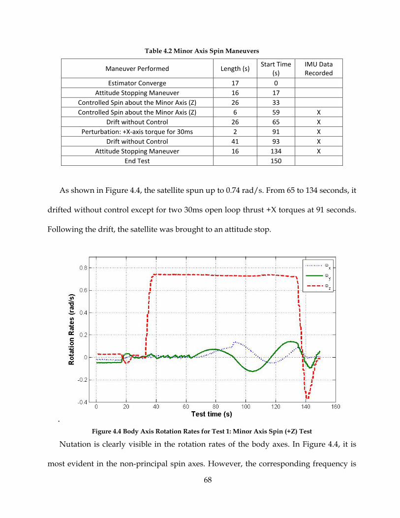
As shown in Figure 4.4, the satellite spun up to 0.74 rad/s. From 65 to 134 seconds, it

drifted without control except for two 30ms open loop thrust +X torques at 91 seconds.

Following the drift, the satellite was brought to an attitude stop.

.

Figure 4.4 Body Axis Rotation Rates for Test 1: Minor Axis Spin (+Z) Test

Nutation is clearly visible in the rotation rates of the body axes. In Figure 4.4, it is

most evident in the non-principal spin axes. However, the corresponding frequency is

69

visible in the principal spin axis (Z) also; there was a peak in the Z-axis rotation rate at

117 seconds, when the phasing of the non-principal axes has them at their combined

lowest. This would be the point when the nutation angle was the smallest; the nutation

angle was at its highest at just before the stopping maneuver (134 seconds).

For this particular test, a full uninterrupted nutation cycle was not observed. At the

nutation frequency observed, just over one cycle could have been observed. However,

the timing of the perturbation, which affects the magnitude and frequency of the

nutation within the rotation rates, interrupted this cycle. Tests following this test session

moved the perturbation to beginning of the drift period, so not to disturb the nutation

cycles, and increased both the principal axis rotation rate and drift period to observe a

greater number of nutation cycles.

The position of the SPHERES satellite moved throughout the entire test. In this

particular case, the satellite moved generally closer to the center of the test volume.

However, had the satellite’s velocity in the Z direction been reversed, it most likely

would have encountered a wall before the completion of the active portion of the test.

70

Figure 4.5 Test 1 Position Location within the ISS Test Volume

Minor Axis Spin (+Z) Test

The processed IMU data in Figure 4.6 matches the rotation rates and nutation values

in the gyroscopic data with that given by the telemetry. The spikes in the accelerometer

data indicate the opening and closing of thrusters. The data shows thruster activity for

the end of the controlled rotation and the attitude hold maneuver at the end of the test.

In between, there is no thruster activity during the long drift period except the two

spikes for the perturbation of two 30ms +X torque separated by 1 second (at ~91

seconds of test time).

(a)

(b)

Figure 4.6 Test 1 IMU 1000Hz data (a) Accelerometers (b) Gyroscopes

71

4.2.2 Intermediate Axis Spin

Test 2 was the only microgravity test that spun about the intermediate principal axis

(+Y). The test was performed twice with very similar results. Therefore, only the first

test execution will be shown here.

As shown in Figure 4.7, the satellite spun up to 1.25 rad/s. From 55 to 262 seconds, it

drifted without control except for a single 30ms open loop thrust +X torque at 58

seconds. Following the drift, the satellite was brought to an attitude stop.

Figure 4.7 Test 2 Body Axis Rotation Rates

Intermediate Axis Spin (+Y) Test

The test was able to maintain the +Y axis as the principal axis of rotation provided

active control was on. Once the active control was turned off, the direction of the

angular momentum vector began moving through the body. This was not the coning

and nutation seen in major or minor axis spin; it was unstable spin. The direction of

spin completely reversed directions four times.

At the time this test was performed, the CAD inertia model was being used as the

reference inertia model, which indicates the Y-axis to be the major axis and the X-axis to

72

be the intermediate axis. That order of the principal axes clashes with the results of this

test.

Following this test, the reference containing the ground measured inertia matrix

model was discovered and it was put into use. These tests correlate with order of axes

in that inertia model, which indicates the Y-axis to be the intermediate axis for the three

SPHERES satellites on the ISS.

4.2.3 Major Axis Spin

Test 3 was the only microgravity test that spun about the major principal axis (+X).

As shown in Figure 4.8, the satellite achieves a spin rate of 1.115 rad/s at 67 seconds

at the end of the controlled rotation period, which is within 0.14 rad/s of the targeted

rotation rate of 1.25 rad/s. A previous attempt of the test attained 1.25 rad/s with a

similar rotation profile just prior to running out of CO2. The impact of the change of the

CO2 tank immediately before this test on the gas levels in the tank and the thruster

value system is assumed to be the cause of the undershooting. The only disruption this

caused was that since the rotation rate was lower, so was the nutation frequency and

there were fewer nutation cycles to observe.

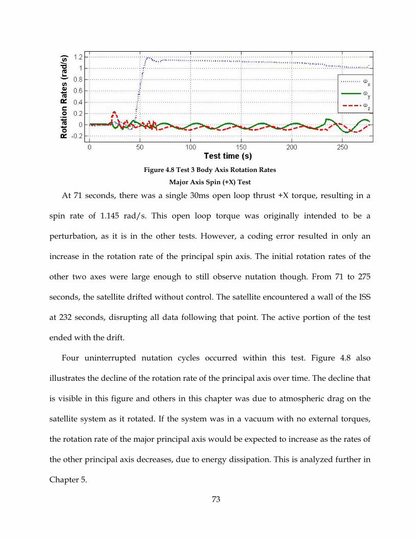
73

Figure 4.8 Test 3 Body Axis Rotation Rates

Major Axis Spin (+X) Test

At 71 seconds, there was a single 30ms open loop thrust +X torque, resulting in a

spin rate of 1.145 rad/s. This open loop torque was originally intended to be a

perturbation, as it is in the other tests. However, a coding error resulted in only an

increase in the rotation rate of the principal spin axis. The initial rotation rates of the

other two axes were large enough to still observe nutation though. From 71 to 275

seconds, the satellite drifted without control. The satellite encountered a wall of the ISS

at 232 seconds, disrupting all data following that point. The active portion of the test

ended with the drift.

Four uninterrupted nutation cycles occurred within this test. Figure 4.8 also

illustrates the decline of the rotation rate of the principal axis over time. The decline that

is visible in this figure and others in this chapter was due to atmospheric drag on the

satellite system as it rotated. If the system was in a vacuum with no external torques,

the rotation rate of the major principal axis would be expected to increase as the rates of

the other principal axis decreases, due to energy dissipation. This is analyzed further in

Chapter 5.

74

4.2.4 Major Axis Spin of the SPHERE + Battery Pack Configuration

There were three tests in which the inertia matrix was altered by adding a solid mass

(battery pack) to the SPHERES satellite (Test 4,5,6). The satellite spun about the major

principal axis of the system (+Y). The primary difference between the tests was the rate

of rotation and they will be identified by that value.

As shown in Figure 4.9, the satellite spun up to 0.74 rad/s for Test 4. From 65 to 134

seconds, it drifted without control except for two 30ms open loop thrust +X torques at

91 seconds. The satellite encountered a wall of the ISS at 112 seconds, disrupting all data

following that point. Following the drift, the satellite was brought to an attitude stop.

Due to the very low nutation frequency observed, a full nutation cycle could not have

been observed even without the disturbances of the perturbation and the wall

encounter.

Figure 4.9 Test 4 Body Axis Rotation Rates

Major Axis Spin of the SPHERES + Battery Pack (+Y) Test: Rotation Rate 0.74 rad/s

As shown in Figure 4.10, the satellite spun up to 1.25 rad/s (Test 5). From 55 to 262

seconds, it drifted without control except for a single 30ms open loop thrust +X torque

75

at 58 seconds. Following the drift, the satellite was brought to an attitude stop. Two full

nutation cycles were observed.

Figure 4.10 Test 5 Body Axis Rotation Rates

Major Axis Spin of the SPHERES + Battery Pack (+Y) Test: Rotation Rate 1.25 rad/s

As shown in Figure 4.11, the satellite spun up to 1.4 rad/s under closed loop control

in Test 6. From 71 to 80 seconds, open loop thrust increased the rotation rate to 6.2

rad/s. From 80 to 282 seconds, the satellite drifted without control. The satellite

encountered a wall of the ISS at 233 seconds, disrupting all data following that point.

The active portion of the test ended with the drift. Eleven full nutation cycles were

observed. The loss of signal (LOS) in broadcast of the video occurred at 175 seconds,

which is why the rotation rate detected by the video ends there (discussed further in

4.2.4.1).

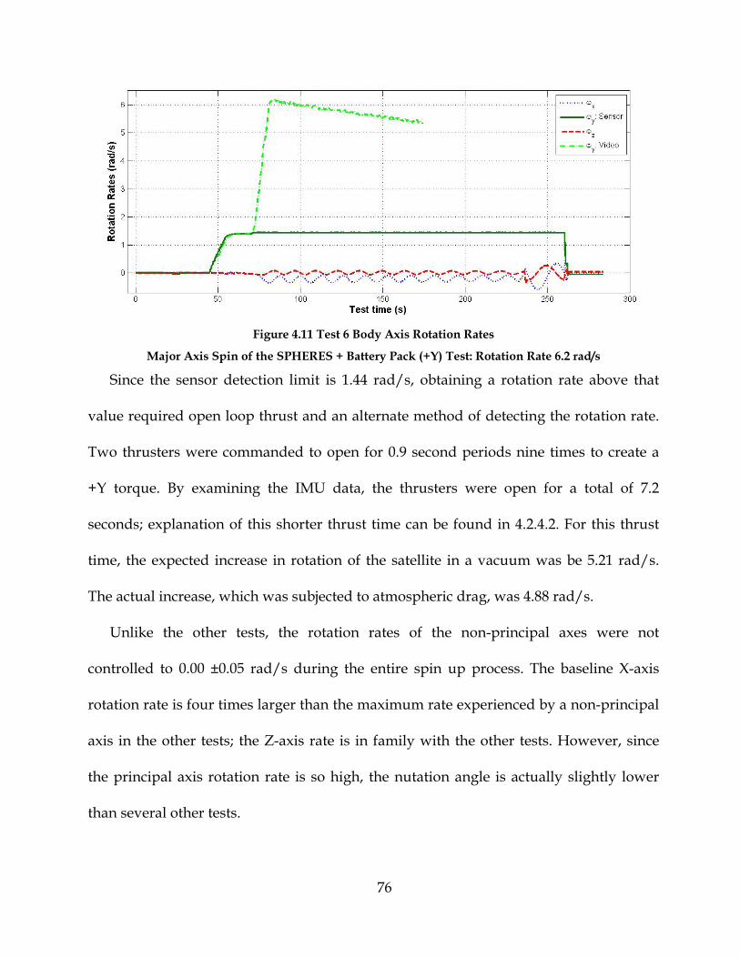
76

Figure 4.11 Test 6 Body Axis Rotation Rates

Major Axis Spin of the SPHERES + Battery Pack (+Y) Test: Rotation Rate 6.2 rad/s

Since the sensor detection limit is 1.44 rad/s, obtaining a rotation rate above that

value required open loop thrust and an alternate method of detecting the rotation rate.

Two thrusters were commanded to open for 0.9 second periods nine times to create a

+Y torque. By examining the IMU data, the thrusters were open for a total of 7.2

seconds; explanation of this shorter thrust time can be found in 4.2.4.2. For this thrust

time, the expected increase in rotation of the satellite in a vacuum was be 5.21 rad/s.

The actual increase, which was subjected to atmospheric drag, was 4.88 rad/s.

Unlike the other tests, the rotation rates of the non-principal axes were not

controlled to 0.00 ±0.05 rad/s during the entire spin up process. The baseline X-axis

rotation rate is four times larger than the maximum rate experienced by a non-principal

axis in the other tests; the Z-axis rate is in family with the other tests. However, since

the principal axis rotation rate is so high, the nutation angle is actually slightly lower

than several other tests.

77

4.2.4.1 Detecting Rotation Rate by Video

In this test, video of the test session was examined to detect principal axis rotation

over the sensor limit. The video was received was from a broadcast during the test

session and LOS are common through test sessions. An LOS occurred from 175 seconds

through the end of the test, which is why there is no available rotation rate data for the

Y-axis during that period.

The satellite was oriented so that during the principal axis spin, the battery pack and

CO2 tank end moved in a circle whose plane was parallel to the camera view. The

battery pack and tank end stuck out at approximately 90˚ from one another. By noting

the frame numbers in which the two items line up either parallel or perpendicular to the

side of the frame, it was possible to determine the frequency of that quarter wavelength

of the rotation.

The uncertainty in rotation rate was the rotation rate divided by the frequency of

frame rate divided by the number of wavelengths. The video received from NASA was

29.97 Hz. However, the effective rate was approximately 15 Hz, as every two frames

were identical. During the drift period, the rotation rate ranged from 5.23-6.2 rad/s,

which means the uncertainty in the rate was 0.35-0.42 radians-wavelength/s. During

the portion of the test where the sensor data is still valid and the rotation rate is

measured by the sensors to be 1.39-1.40 rad/s, error in the video data was within the

predicted uncertainty of 0.12 rad/s when calculated at every three-fourths of a

wavelength length. Calculating the rotation rate for wavelengths less than three-fourths

resulted in errors significantly exceeding that of the predicted uncertainty (i.e. error was

78

twice the uncertainty at half a wavelength). This indicates that three seconds of data are

necessary in this test for the error to be within the predicted uncertainty.

For Figure 4.11, the rotation rate during the drift was calculated every half a

wavelength over a two and a half wavelength period. The uncertainty of the average

rotation rate for the entire period was 0.17 rad/s. The disadvantage with averaging the

rotation rate over a period so that uncertainty is known is that the ability to view

fluctuations (i.e. the 23 second nutation cycles) within the rotation rate is reduced.

However, these fluctuations were already difficult to detect due to the uncertainty and

declining rate due to drag. The PSDs of the rotations rates from 85 to 175 seconds are

shown in Figure 4.12. The figure illustrates how the nutation frequency dominates the

non-principal axes frequency spectrums, but not for the principal axis rotation rate

measured via video. Reducing the period of averaging the rotation rate from 2.5 to 1

wavelength did not cause the nutation frequency to peak on the PSD to appear.

(a) (b) (c)

Figure 4.12 Test 6 Power Spectral Density of the Body Axis Rotation Rates

Major Axis Spin of the SPHERES + Battery Pack (+Y) Test: Rotation Rate 6.2 rad/s

(a) X-axis (b) Y-axis (c) Z-axis

4.2.4.2 Open Loop Thrust Anomaly

During Test 6, one or more of the thrusters did not fire as commanded. This

occurred during the open loop thrusting portion of the test. During this part of the test,

79

two of the twelve thrusters were commanded to be open for 0.9 seconds out of every

second for a 9 second period.

The thruster commands recorded match the expected firing of two X-axis direction

thrusters, whose combined theoretical thrust results in Y-axis torque with no net force

(Figure 4.13). The commanded thrust was to occur 0.9 seconds of every second. The

accelerometers experienced a disturbance every time the thrusters opened or closed.

The accelerometer data for this portion of the test is shown in Figure 4.14. During the

first commanded thrust of 0.9 seconds, the thrusters were open for 0.9 seconds. During

the following six commanded thrusts of 0.9 seconds, the thrusters were open for only

0.81 seconds. This shows that by commanding the thrusters to open and close once each

per second, the maximum time that the thrusters can remain open is 0.81 seconds.

However, there was unexplained disruption in the thruster firings at the end of the

open loop thrusting, as shown in Figure 4.14. From time 71 – 78 seconds, the

disturbance forces occurred in the expected pattern. During the eighth thrust cycle,

there were two additional disturbances, as if one or both thrusters closed and then

reopened during the middle of a period when the thruster should have continually

remained open. An astronaut not running the test took a picture during at

approximately this time; this was the only noted variant at the time of the anomaly

from the previous 7 seconds.

80

Figure 4.13 Test 6 Thruster Commands

Figure 4.14 Test 6 Disrupted IMU Data

By examining the position and rotation rates of the body axes at this point, there was

no obvious disruption. It is assumed that both thrusters simultaneously opened and

closed. This would reduce the total time exerting the torque force to increase rotation

rate, but have no other discernable effects. The actually increase in rotation rate was

81

93% that it would have been had this anomaly not occurred. With this being a physical

test, it was more important to know the torque exerted and the resulting rotation rate

than actually reaching a specific rotation rate. The results of the test were not affected

by this anomaly.

4.2.5 Modifications of the Tests

Most of the modifications of the test format happened following the first test session.

Of the three test sessions in which these tests took place, Tests 1 and 4 took place in the

first one; Tests 2 and 5 took place in the second one; and Tests 3 and 6 took place in the

third test session.

4.2.5.1 Adding the Position Holds

In the first test session, the position of the SPHERES satellite is never controlled. The

astronaut placed the satellite in the middle of the test volume with as little initial

velocity as possible. For this experiment, the position is insignificant provided that is

has minimal change and the SPHERES satellite is not near the bounds of the test

volume. However, as found in Figure 4.15, the satellite is capable of reaching these

bounds and encountering a wall (115 seconds) during this period.

The combination of the initial velocity acquired during initial placement in the

volume, the velocity due to uneven thruster force during the controlled rotation from

33-60 seconds, and the velocity due to any air currents within the ISS imparted enough

velocity for the satellite to impact the wall of the ISS for this particulate test run. Once

this occurred, all test data following that point was not relevant, due to the significant

external force. Since the two previous attempts of the test experienced satellite resets

82

which interrupted the test or the data and it was necessary at that point to move on to

another test within the test session, this test was limited in useable data collected. Since

the nutation frequency was quite low, an entire nutation cycle was not captured in the

data.

Figure 4.15 Test 4 Position and Velocity Data

Major Axis Spin of the SPHERES + Battery Pack (+Y) Test: Rotation Rate 0.70 rad/s

The other test sessions (Tests 2,3,5,6) employed a position hold during all controlled

portions of the test. This way the velocity due to the three factors was minimized up

until the point that control was stopped. The addition of the position did not stop the

problem, as Figure 4.16 illustrates at 230 seconds. However, it did extend the length of

time that the SPHERES satellite could drift while rotating from 50 to 165 seconds.

83

Figure 4.16 Test 3 Position and Velocity Data

Major Axis Spin (+X) Test

It is noted that over half of the tests from all sessions were able to run through

completion without encountering the wall or other obstacles in the ISS. Two runs of the

exact same test were performed one after another, with nearly identical initial

positioning; however, the path of the satellite varied for both. Though the addition of

position hold during controlled rotation increases the time before the satellite could

encounter an obstacle, any future experiments should consider or watch for

opportunities to reduce the position drift when the satellite is not being controlled.

4.2.5.2 Removing stopping maneuver

In the first two test sessions, there is a maneuver at the end of the test that brings the

satellite to an attitude hold. The original intention of this maneuver is to cause whatever

fluid is within the CO2 tank to slosh. However, the control system was imparted and the

noise from use of the estimator overwhelms what fluid slosh may be occurring. It was

84

removed from the diagnostic tests performed in this study to allow more time for the

drift and therefore nutation cycles.

For future experiments with additional fluid tanks, the stopping maneuver could be

imparted with open loop thrusting, removing the noise from the estimator. However,

other disturbances with this method will have to be considered, such as the uneven

thruster forces.

4.2.5.3 Reducing time of IMU

The first test session recorded 1000Hz data from the gyroscope and accelerometer

sensors, beginning with the last 5 seconds of controlled rotation through the end of the

test. This is very costly in terms of test time, as the time to download the 1000 Hz data is

approximately four times the length of time the data was taken over (i.e. 15 seconds of

1000Hz data requires one minute of data download time). For the other test sessions,

1000Hz data was recorded beginning with the last 5 seconds of controlled rotation

through the first 10 seconds of the drift period. This allowed for the length of the drift

period to be increased without causing the length of the test to increase by five times

that time increase.

85

Chapter 5

Model Correlation

This chapter demonstrates that the horizontal slosh ground tests successfully

correlated to previous experimental studies. The angular momentum and nutation

frequency are used for the SPHERES Nutation in Microgravity tests to derive new

inertia models for the SPHERES satellites. The Nutation Time Constant is also examined

for the microgravity tests.

5.1 Horizontal Fluid Slosh Ground Tests

5.1.1 Frequency Modes

5.1.1.1 Previous Experimental Study

The results of this study were correlated to the experimental study performed by

McCarty and Stephens [5]. In that study, horizontal cylindrical containers were agitated

at gradually increasing frequencies until a modal frequency appeared and continued to

resonant even without excitation. The containers in this study are cylinders with some

86

imperfections, within the same radius to length ratios as McCarty and Stephens, and

half the actual length. The fluid in both studies was water.

The equations below refer to the experimentally determined fluid frequency

parameter, , and can be used to calculate the natural modes of a horizontal cylinder

among different acceleration value. Equation 5.1 is for longitudinal modes and Equation

5.2 is for transverse modes. The bottle length and the height of the liquid within the

container are referenced. The frequency parameter for longitudinal modes found by

McCarty and Stephens are shown with the results of this study in Figure 5.1.

5.1

5.2

For Equation 5.2, Equation 5.3 and Figure 5.1, R refers to the radius of the cylinder.

For all other references to R within this study, R refers to the distance of from the center

of mass of a system to the center of mass of the fluid container.

For case of h = R, Lamb applied the first transverse natural frequency in the

equation below [26]. For Container B, the estimated first transversal natural frequency is

0.32 Hz, about a quarter of the first longitudinal natural frequency.

5.3

5.1.1.2 Correlation of Experiments

The longitudinal modes of the horizontal slosh tests are shown in Figure 5.1. The

results are shown for the first longitudinal mode of each container, along with the faired

curves of the parameter for the first four longitudinal modes from [5]. The uncertainty

87

in frequency and imperfections in the cylinders of this study account for the small

variances from McCarty and Stephens. The method in this study of obtaining modes in

containers with liquid is verified.

Figure 5.1 Experimental 1st Longitudinal Modes

Once the fluid frequency parameters are found here on Earth, they can be used to

find the modal frequencies elsewhere by substituting the gravity term with the

dominate acceleration source. On a spinning spacecraft in microgravity, this will be

centrifugal force. Since the replacement of the acceleration force for gravity is , a

container for a given fill level will have its natural frequency by directly proportional to

the spin rate, just like the nutation frequency.

5.4

Assuming the offset tanks are 12.5 cm from the center of mass of the system and the

system is accelerating at 1.25 rad/s, the acceleration exerted on the tanks will go from

88

9.807 m/s to 0.0195 m/s. The modal frequencies would be expected to decrease to

approximately 4.5% of their values on Earth.

5.1.2 The Effect of Fill Fraction on Slosh Power

The force power is expected to increase both with increased fluid mass and

increased draw back distance. However, the force power peaks at the 68% fill level

Container A and the 50% fill level Container B, as shown in Figure 5.2. This is because

the largest slosh mode/resonance is at this fill fraction; the largest active component of

fluid occurs at this fill. Though the higher fill fractions have more overall fluid mass, a

lower percentage of that mass is participating in the mode such that the amount of

active mass is smaller.

Figure 5.2 Liquid Fill Fraction vs. Power Density of the 1st Longitudinal Mode

These power values are associated with the frequency that is the first longitudinal

mode. This mode has the highest PSD for fill fractions between 20-90%; the outlying fill

fractions had much higher frequencies than the highest PSD, but they were on the same

order of magnitude as the PSD of the first mode. For Container B, the draw-back

distance shown in Figure 5.2 is constant at 10 cm. The Container A distances were kept

89

approximately constant, but were not as rigorously controlled. This is why the trend in

maximum power density is less ordered.

To determine the peak slosh power fill fraction, there should be greater detail

around the fill fractions that have the highest power densities. The expected peak in

active fluid is expected at ~60%.

5.1.3 Applicability

The horizontal slosh tests demonstrate a method of determining slosh frequency

modes and the power associated with them. The tests match other experimental results

of a horizontal cylindrical container with water. By altering the container with hemi-

spherical ends and/or changing the fluid within the container, the ability to correlate

with McCarthy and Stephens will wane. However, the new container(s) can be tested

with the method established here to find its longitudinal modes, along with which fill

fractions result in the highest slosh power for that container and fluid.

The method can also be altered so that transverse modes can be obtained. The main

difference will be the side of the container contacting the load cell will switch, which

will require set-up changes to accommodate.

However long the test is following shock event, 1/test length is the uncertainty that

will result. For example, if the usable test data following the shock event is 5 seconds,

then the PSD values are available at 0.2 Hz increments. Test data in this study results in

frequency increments ranging from 0.25-0.4 Hz. This was caused by a coding issue in

the test set-up for recording data that resulted in only 10 seconds of data per test. This

90

issue was not overcome at the time of the tests, but is expected to not be difficult to

work through in the coding of the recording software.

The larger drawback tests had shorter usable test data, since it took the fluid longer

to recover from the shock event, and so have larger uncertainty. Since the lower

frequencies are of greater interest, it is vital to increase the time length of the usable

data. By removing the restriction of the amount of time to end data recording, the

amount of data following the shock event can increase and the fidelity in frequency

modes will significantly increase.

The highest detectable frequency will be half of that data rate on the sensor. In this

case, the sensor data rate was 1000 Hz, and 500 Hz is significantly higher than the

frequencies of interest.

5.1.4 Angular Momentum Conservation and the Drag Effect

The drag force for the Z-axis is lower than that exerted on the other two axes. Since

this is an external torque that acts as a disturbance to the test, it is preferable to

minimize the drag when possible.

In the current configuration of the SPHERES satellite, the only practical locations to

add mass to the system at the +X and –X faces of the satellite, since the Y faces are

hinged battery doors and the Z faces have the tank and pressure knob protruding from

the satellite. As the result, the moment of inertia (MOI) about the X-axis would only

increase minimally compared to the MOIs about the Y-axis and Z-axis. When adding

masses to the system, the impact on the MOIs must always be considered. For studies

91

involving gyroscopic spin, the axis of the spin can never be the intermediate axis, due to

its inherent instability.

For the cylindrical offset fluid tanks this study is addressing, the symmetric axis of

the tank is in-line with the axis of spin of the satellite. This orientation must be

considered in determining the MOI of the new system. If the tanks are placed at the –X

and +X faces in-line with Y-axis, the increase in the MOIs is greatest in Z-axis direction

and least in the X-axis direction. If in-line with the Z-axis, then the Y-axis MOI will have

the greatest increase and the X-axis will remain the least. This allows two options for

spin axis:

• Y-axis rotation (major axis spin), provided the increase in the Y-axis MOI

overcomes the X-axis MOI and the Z-axis MOI does not overcome the Y-axis

MOI

• Z-axis rotation (minor axis spin), provided the increase in the Z-axis MOI does

not overcome the X-axis MOI (unlikely for the Z-axis MOI to overcome the Y-axis

MOI)

The inertia of the fluid tanks, including fluid within the tank, will dictate which, if

either, of these options is possible. For tanks designed to be added to the system, this

should be taken into consideration, to avoid instable spin occurring during the test.

If both axes could be spun about without being the intermediate axis, the Z-axis is

preferable so that the drag on the system is minimized. However, the drag due to the

addition of the fluid tanks will have to be calculated for all configurations used.

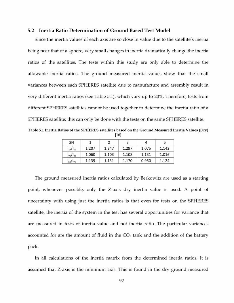
92

5.2 Inertia Ratio Determination of Ground Based Test Model

Since the inertia values of each axis are so close in value due to the satellite’s inertia

being near that of a sphere, very small changes in inertia dramatically change the inertia

ratios of the satellites. The tests within this study are only able to determine the

allowable inertia ratios. The ground measured inertia values show that the small

variances between each SPHERES satellite due to manufacture and assembly result in

very different inertia ratios (see Table 5.1), which vary up to 20%. Therefore, tests from

different SPHERES satellites cannot be used together to determine the inertia ratio of a

SPHERES satellite; this can only be done with the tests on the same SPHERES satellite.

Table 5.1 Inertia Ratios of the SPHERES satellites based on the Ground Measured Inertia Values (Dry) [16]

SN 1 2 3 4 5 Ixx/Izz 1.207 1.247 1.297 1.075 1.142

Iyy/Izz 1.060 1.103 1.108 1.131 1.016

Ixx/Iyy 1.139 1.131 1.170 0.950 1.124

The ground measured inertia ratios calculated by Berkowitz are used as a starting

point; whenever possible, only the Z-axis dry inertia value is used. A point of

uncertainty with using just the inertia ratios is that even for tests on the SPHERES

satellite, the inertia of the system in the test has several opportunities for variance that

are measured in tests of inertia value and not inertia ratio. The particular variances

accounted for are the amount of fluid in the CO2 tank and the addition of the battery

pack.

In all calculations of the inertia matrix from the determined inertia ratios, it is

assumed that Z-axis is the minimum axis. This is found in the dry ground measured

93

inertia values for all SPHERES satellites tested in microgravity for this study; the

addition of CO2 fluid increases the inertia in the other two axes more than the Z-axis

and keeps it the minor axis. When adding mass on both the +X and –X face (i.e. a

battery pack or fluid tank on each side), it is possible for the Z-axis to overcome one of

the other axes in MOI and become the intermediate axis.

5.3 Nutation Frequency of ISS Tests

The nutation frequencies of the tests compared the predicted frequencies based off

of the ground measured inertia model vary significantly from the test results, as shown

in Table 5.2.

Table 5.2 Nutation Frequency of Each Test

Test System Axis of

Rotation

Initial Rotation Rate

Ω: rad/s

Nutation Frequency λ: rad/s

λ / Ω

Predicted Test Predicted Test

1 SPHERE

Z 0.74 0.126 0.103 0.171 0.139 2 Y 1.25 imag imag imag imag 3 X 1.15 0.275 0.194 0.239 0.168 4

SPHERE + Battery Pack

Y 0.74 imag 0.052 imag 0.070

5 1.25 imag 0.087 imag 0.070 6 6.28 imag 0.459 imag 0.073

A major difference between the predictions and the test results is that the ground

measured model has the difference between the X-axis and Y-axis great enough that

even with the addition of the battery pack, the Y-axis remains the intermediate axis.

However, the tests demonstrate that the battery pack causes the Y-axis to be the major

axis for all SPHERES satellites.

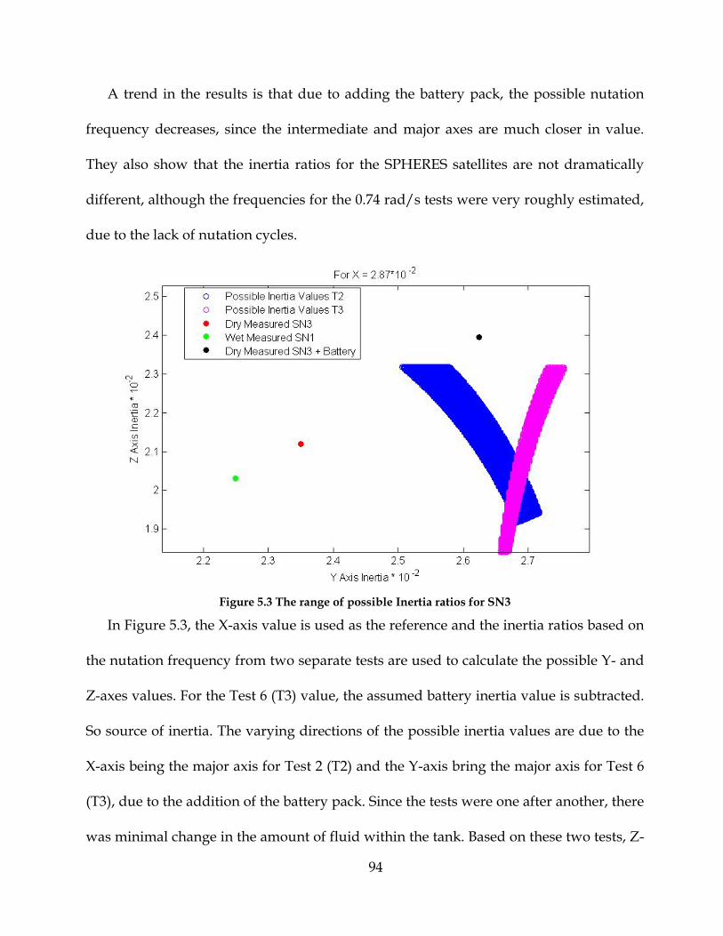
94

A trend in the results is that due to adding the battery pack, the possible nutation

frequency decreases, since the intermediate and major axes are much closer in value.

They also show that the inertia ratios for the SPHERES satellites are not dramatically

different, although the frequencies for the 0.74 rad/s tests were very roughly estimated,

due to the lack of nutation cycles.

Figure 5.3 The range of possible Inertia ratios for SN3

In Figure 5.3, the X-axis value is used as the reference and the inertia ratios based on

the nutation frequency from two separate tests are used to calculate the possible Y- and

Z-axes values. For the Test 6 (T3) value, the assumed battery inertia value is subtracted.

So source of inertia. The varying directions of the possible inertia values are due to the

X-axis being the major axis for Test 2 (T2) and the Y-axis bring the major axis for Test 6

(T3), due to the addition of the battery pack. Since the tests were one after another, there

was minimal change in the amount of fluid within the tank. Based on these two tests, Z-

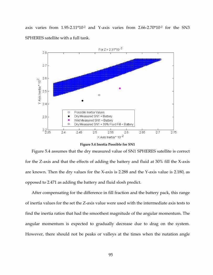
95

axis varies from 1.95-2.11*10-2 and Y-axis varies from 2.66-2.70*10-2 for the SN3

SPHERES satellite with a full tank.

Figure 5.4 Inertia Possible for SN1

Figure 5.4 assumes that the dry measured value of SN1 SPHERES satellite is correct

for the Z-axis and that the effects of adding the battery and fluid at 30% fill the X-axis

are known. Then the dry values for the X-axis is 2.288 and the Y-axis value is 2.180, as

opposed to 2.471 as adding the battery and fluid slosh predict.

After compensating for the difference in fill fraction and the battery pack, this range

of inertia values for the set the Z-axis value were used with the intermediate axis tests to

find the inertia ratios that had the smoothest magnitude of the angular momentum. The

angular momentum is expected to gradually decrease due to drag on the system.

However, there should not be peaks or valleys at the times when the nutation angle

96

increases (i.e. when the rotation rate of the spin axis is at its lowest in the nutation

cycle).

Figure 5.5 shows the angular momentum magnitude with the ground measured

inertia values and with the inertia values from Figure 5.4 adapted from the major axis

spin with the battery pack that results in the lowest magnitude of peaks/valleys.

Figure 5.5 Angular Momentum Magnitude of the Test 2 for both the Ground and ISS Measured Inertia

Values

The method of optimizing the inertia ratios to best fit the magnitude of angular

momentum does not work for other cases besides the intermediate axis spin. Since the

intermediate axis spin is unstable, the satellite switches principal axes of rotation

throughout the test and each axis crosses the zero value at least once in the test. The

dramatic switching of axes allows for definite viewing of magnitude changes in the

angular momentum vector that are due to inaccurate inertia ratios and not disturbances

of the physical system.

In the minor/major axis spin tests, the peaks and valleys in the magnitude of

angular momentum over time due to nutation are visible, but only slightly. Table 5.3

shows the calculated ISS best estimates of inertia of SPHERES satellite SN1 and SN3

97

with the applicable fill fraction, based on all tests. Tests 1 and 4 were performed on SN2

and the data collected did not allow for calculation of the inertia matrix of that

particular SPHERES satellite.

Table 5.3 ISS Measured Inertia Values

SN Fill Fraction of

CO2 Tank (kg m2)*10-2

Ixx Iyy Izz

1 Dry 2.3245 2.2174 1.9509 48% 2.4357 2.3021 1.9509

30% + Battery 2.4939 2.5443 2.2259

3 Dry 2.7350 2.5365 2.0248 68% 2.8550 2.6565 2.0248

65% + Battery 2.8640 2.9305 2.2998

5.4 Nutation Time Constant Calculation

For major axis spin of the SPHERES satellite only (Test 3), the maximum nutation

angle increases from 0.0715 to 0.073 radians from 92 seconds to 189 seconds (see Figure

5.6 (a)), resulting in a Nutation Time Constant (NTC) of 4672. Since the NTC is positive,

this indicates that the nutation angle is growing, which is the opposite of what is

expected for spin about a major axis. For that NTC, the nutation angle doubles every

3238 seconds.

98

(a) (b)

(c)

Figure 5.6 Nutation Angle of (a) Test 3: Major Axis Spin (+X) Test (b) Test 5: Major Axis Spin of the SPHERES + Battery Pack (+Y) Test: Rotation Rate 1.25 rad/s (c) Test 6: Rotation Rate 6.28 rad/s

For major axis spin of the SPHERES satellite with battery pack at 1.25 rad/s (Test 5),

the maximum nutation angle decreases from 0.0719 to 0.0708 radians from 80 to 224

seconds (see Figure 5.6 (b)), resulting in a NTC of -9340. Since the NTC is negative, this

indicates that the nutation angle is decaying, which is as expected for spin about a

major axis. For that NTC, the nutation angle halves every 6474 seconds.

When examining the nutation angle for every cycle, in both tests, the nutation angle

goes both up and down. However, the NTCs listed above show the general trend for

those tests.

99

This system has a prominent external force in the atmospheric drag and it does not

affect the rotation rates about all axes the same. The drag is proportional to the square

of the velocity, so the axes spinning faster will also not decrease at linearly the same rate

as the slower spinning axes. Also, since the coefficient of drag is different for the axes,

some will slow down faster than others. In the major axis spin of the SPHERES satellite

only test, the coefficient of drag on the Z-axis is significantly lower than that of either

the X- or Y-axis, and apparently that factor combines with the lower velocity to increase

the nutation angle instead of decreasing it, as the inertia matrix of the SPHERES satellite

would suggest. The major axis spin of the SPHERES satellite with altered inertia matrix

at 1.25 rad/s test (Test 5) adds a battery pack to the SPHERES satellite. This would

expectedly increase the coefficient of drag on all axes, but would have the greatest effect

on the Z-axis. This evening out allows the inertia matrix to dominate over the

atmospheric drag in effect on the nutation angle growth/decay.

5.5 Open Loop Thrust

Torque is calculated from the cross product of the displacement vector and

the force vector . For calculating the open loop thrust of the SPHERES satellite, the

displacement vector is the distance from the center of mass to the location of each firing

thruster. The force vectors due to each thruster are assumed to be only in the Y plane

(i.e. force vectors out of the Y plane are negligible). For constant torque, the angular

acceleration is also constant and can therefore be used to find the angular velocity.

5.5

100

5.6

Table 5.4 Various Calculations of Rotation Rate Increase

Model for Iyy Used Angular Acceleration Increase in

Angular Velocity

rad/s2 rad/s Ground Measured SN3 Full Tank + Battery 0.942 6.78

ISS Measured SN3 Full Tank + Battery 0.723 5.21 Test (Actual) 0.678 4.88

The results in Table 5.4 show how much closer the ISS Measured Inertia Values

calculated increase in angular velocity is to the actual increase produced by open loop

thrust than that calculated by the Ground Measured Inertia Values. The difference

between the ISS Measured Inertia Values calculated increase in angular velocity and the

actual increase in angular velocity are assumed to be due to thruster variance and

atmospheric drag.

While the SPHERES satellite is in controlled rotation, the X- and Z-axis rotation rates

are controlled to within 0.05 rad/s of 0.00 rad/s. Therefore, when the control is turned

off and the SPHERES satellite is drifting, the centerline of the rotation rate for those axes

is expected to be -0.05 to 0.05 rad/s. This occurs for all other tests, except for tests in

which the rotation rate is set with an open loop thrust instead of closed loop estimation.

101

Chapter 6

Conclusions

This chapter includes the summary of this thesis and its contributions. It also makes

recommendations for future work for this study.

6.1 Thesis Summary

This thesis discusses the issues involving fluid slosh and nutation on spinning

spacecraft pertaining to prediction. It develops an approach to perform fluid slosh tests

in microgravity on a simplified spacecraft system by using the SPHERES Testbed on the

ISS. The work performed characterizes the nutation of the SPHERES satellite and the

environment of testbed in preparation for performing spinning tests on the SPHERES

with fluid tanks attached. The work also includes horizontal testing of fluid tanks on

the ground, as a method of characterizing the fluid slosh frequencies of a tank prior to

testing in microgravity (on the ISS).

102

6.2 Contributions

This work developed and verified a method of fundamental frequency

determination of a fluid tank in a ground based lab. It has determined the inertia

properties of the SPHERES satellites in microgravity. It also characterized the ISS

environment and expected external disturbances. This will allow for future physical

tests to better understand the mass properties of the spacecraft and the abilities of the

SPHERES satellites to perform physical tests.

6.3 Future Work

This study can be continued by conducting microgravity tests with fluid tanks

attached. There are two options for fluid tanks, based on the guidelines set for testing

on the ISS: SPHERES CO2 tanks and fluid tanks sent up to the ISS. Both of these tanks

will need to be ground tested to determine their slosh frequencies prior to testing on the

ISS.

By testing the fluid containers on Earth and knowing the expected location of the

container and spin rate on the SPHERES satellite, the tests will be able to determine the

first modes of longitudinal and transverse slosh expected to be observed in

microgravity. These tests can then determine if slosh is expected to resonate with

nutation and which mode it will be, or preferable use this information to develop tanks

with fluid levels that will produce slosh to resonate with the nutation.

If possible, conduct the ISS tests with the SPHERES on-axis propellant CO2 tank

nearly empty. This will reduce its effect on the system, so that the attached off-set fluid

tank(s) is the main contributor to the energy dissipation. Also, test on the ISS both with

103

the off-set tank empty or with a rigid mass inside in addition and with fluid in the tank.

This allows observation of the effect of adding the mass of the tanks along with the

increased atmospheric drag, with and without the motion due to the fluid.

1. Horizontal Slosh Ground Tests

• Perform on containers intend to use as offset spinners on ISS (CO2 or designed)

o Longitudinal

o Lateral

• Make sure to:

o Test heavily around fill fraction intended for use on ISS (i.e. test at a

greater frequency in the range of fill fractions near the ISS fill fraction

than for fill fractions outside of that range).

o Collect data over a time length adequate to view low frequencies

2. Characteristics of the Instrumented Fluid Tanks (to be sent to ISS and then attached

to SPHERES satellites for slosh testing)

• Clear, to be able to see the slosh occurring in the tanks

• Specially machined, to be able to choose a tank shape that will best correlate to

the tank of interest (i.e. launch vehicle or spacecraft tanks)

• Filled with specified fluid, to be able to choose a fluid for correlation to a chosen

launch vehicle or spacecraft fluid and possibly color for viewing the slosh

• Have attach points, to be able to have the best connection to the SPHERES

satellite and reduce disturbances to the system and attenuation of the slosh

forces to the sensors due to attachment

104

• Contain greater fluid than currently present in the SPHERES satellite, to be able

to increase effect of slosh on the satellite

• Have sensors with capabilities beyond those present on the SPHERES satellites,

to be able to better observe the fluid slosh

105

Bibliography

[1] Raouf A. Ibrahim, Liquid sloshing dynamics : theory and applications. New York:

Cambridge University Press, 2005.

[2] Spyros A Karamanos, Lazaros A Patkas, and Manolis A Platyrrachos, "Sloshing Effects

on the Seismic Design of Horizontal-Cylindrical and Spherical Industrial Vessels,"

Journal of Pressure Vessel Technology, vol. 128, 2006.

[3] S Papaspyrou, D Valougeorgis, and S A Karamanos, "Sloshing Effects in Half-Full

Horizontal Cylindrical Vessels Under Longitudinal Excitation," Journal of Applied

Mechanics, vol. 71, 2004.

[4] Lazaros A Patkas and Spyros A Karamanos, "Variational Solutions for Externally

Induced Sloshing in Horizontal-Cylindrical and Spherical Vessels," JOURNAL OF

ENGINEERING MECHANICS, 2007.

[5] John McCarty and David G Stephens, "Investigation of the natural frequencies of a

fluid in spherical and cylindrical tanks," Langley Research Center, Washington, NASA

Technical Report NASA TN D-252, 1960.

[6] Carl Hubert, "Behavior of Spinning Space Vehicles with Onboard Liquids,"

NASA/Kennedy Space Center, Purcellville, Technical Report B3007; Contract Number

106

NAS10-02016, 2008.

[7] Alvar Saenz-Otero, "The SPHERES Satellite Formation Flight Testbed: Design and

Initial," Electrical Engineering and Computer Science, Masschusetts Institute of

Technology, Cambridge, Masters Thesis 2000.

[8] Mark O Hilstad, John P Enright, Arthur G Richards, and Swati Mohan, "The SPHERES

Guest Scientist Program," Space Systems Laboratory, Massachusetts Institute of

Technology, SPHERES GSP version 2.1, 2010.

[9] ISS Expedition 14 Crew, SPHERES Satellite Image Taken Aboard ISS, 2007.

[10] J.M.A. Danby, Fundamentals of Celestial Mechanics, 2nd ed. Richmond, VA: Willmann-

Bell, Inc, 1992.

[11] Computer Sciences Corporation: Attitude Systems Operation, Spacecraft Attitude

Determination and Control, James R. Wertz, Ed. Boston: Kluwer Academic Publishers,

2002, vol. 73.

[12] Michael T. Kezirian, "Fuel Slosh Dynamics in Spinning Spacecraft," in 42nd

AIAA/ASME/SAE/ASEE Joint Propulsion Conference & Exhibit, Sacramento, CA, 2005, p.

8.

[13] Keith Schlee, Sathya Gangadharan, and James Ristow, "Parameter Estimation of

Spacecraft Fuel Slosh," in 47th AIAA/ASME/ASCE/AHS/ASC Structures, Structural

Dynamics, and Materials Conference, Newport, RI, 2006, p. 18.

[14] Launch Services Program. (2002) Kennedy Space Center Research and Technology

Reports. [Online].

http://rtreport.ksc.nasa.gov/techreports/2002report/300%20Range%20Tech/306.html

[15] Allen Chen, "Propulsion System Characterization for the SPHERES Formation Flight

and Docking Testbed," Aeronautics and Aeronautics, Massachusetts Institute of

107

Technology, Cambridge, MA, Masters Thesis 2000.

[16] Dustin Berkovitz, "System Characterization and Online Mass Property Identification of

the SPHERES Formation Flight Testbed," Aeronautics and Astronautics, Massachusetts

Institute of Technology, Cambridge, MA, Masters Thesis SSL# 26-07, 2007.

[17] "SPHERES ISS Test Session 14," Space Systems Laboratory, Massachusetts Insititute of

Technology, Cambridge, MA, Test Session Plan 2008.

[18] Johnson Space Center, "Joint Crew Provisioning Catalog," National Aeronautics and

Space Administration, Houston, SSP 50477; Rev A, 2007.

[19] Jr., John D Anderson, Fundamentals of Aerodynamics.: McGraw-Hill, 2003.

[20] Aurora Flight Systems, Inc, SPHERE Assembly.

[21] Principal Investigator Microgravity Services (PIMS). [Online].

http://pims.grc.nasa.gov/html/ISSAccelerationArchive.html

[22] Walter Tam, Sam Wiley, Katherine Dommer, Larry Mosher, and David Persons,

"Design and Manufacture of the MESSENGER Propellant Tank Assembly," in 38th

AIAA/ASME/SAE/ASEE Joint Propulsion Conference & Exhibit, 2002.

[23] D.O. Lomen, "Digital Analysis of Liquid Propellant Sloshing in Mobile Tanks with

Rotational," NASA CR-230, 1965.

[24] D.O. Lomen, "Liquid Propellant Sloshing in Mobile Tanks with Rotational Symmetry,"

CR-222, 1965.

[25] Gilbert Strang, Computational Science and Engineering. Cambridge, MA: Wellesley-

Cambridge Press, 2007.

[26] Stefan aus der Wiesche, "Sloshing dynamics of a viscous liquid in a spinning horizontal

cylindrical tank," Aerospace Science and Technology, vol. 12, no. 6, 2008.

108

[27] Carl Hubert, "Introduction to the Dynamics & Control of Spinning Space Vehicles,"

West Windsor, 2001.

[28] Marco B. Quadrelli, "Nutation Time Constant Determination of On-Axis Diaphragm,"

Journal of spacecraft and rockets , vol. 42, no. 3, 2005.

[29] JetStream - Online School for Weather. [Online].

http://www.srh.noaa.gov/jetstream/atmos/pressure.htm

[30] Southwest Research Institute, "The Dynamics Behavior of Liquids in Moving

Containers," Scientific and Technical Information Division, National Aeronautics and

Space Administration, Washington, DC, NASA SP-106, 1966.

[31] Franklin T. Dodge, "The New Dynamics of Liquids in Moving Containers," Southwest

Research Institute, San Antonio, TX, 2000.

[32] Keith Schlee and James Sudermann, "Estimation of Nutation Time Constant Model

Parameters for On-Axis Spinning Spacecraft," in AIAA/AAS Astrodynamics Specialist

Conference and Exhibit, 2008.

[33] Gilbert Strang, Introduction to Applied Mathematics.: Wellesley-Cambridge Press, 1986.

[34] Ja-Young Kang, "Slosh Dynamics of Internal Mass in a Spinning Vehicle," in AIAA/AAS

Astrodynamics Specialist Conference and Exhibit, Providence, RI, 2004, p. 11.

[35] R.J. Hung, Y.T. Long, and Y.M. Chi, "Slosh Dynamics Coupled with Spacecraft Attitude

Dynamics; Part 1: Formulation and Theory," Journal of Spacecraft and Rockets, vol. 33, no.

4, p. 7, July-August 1996.

[36] Ja-Young Kang and John E Cochran Jr., "Stability Criteria of Slosh Motion with

Periodicity in a Spinning Spacecraft," Journal of Guidance, Control and Dynamics, vol. 28,

no. 3, p. 6, May-June 2005.