nyu wireless tr 20 15 -00 2wireless.engineering.nyu.edu/static-homepage/tech-reports/tr2015... ·...
TRANSCRIPT
© 2015 NYU
NYU WIRELESS TR 2015-002 Technical Report
Indoor Office Wideband Millimeter-Wave Propagation Measurements and Channel Models at 28 GHz and 73 GHz for Ultra-
Dense 5G Wireless Networks
Results published in:
G. R. MacCartney, Jr., T. S. Rappaport, S. Sun, and S. Deng, “Indoor Office Wideband Millimeter-Wave Propagation Measurements and Channel Models at 28 GHz and 73 GHz for Ultra-Dense 5G Wireless
Networks, (Invited Paper),” IEEE Access, 2015.
George R. MacCartney, Jr., Sijia Deng, Shu Sun, and
Theodore S. Rappaport [email protected], sijia @nyu.edu, ss7152@nyu, and [email protected]
NYU WIRELESS NYU Polytechnic School of Engineering
2 MetroTech Center Brooklyn, NY 11201
Oct. 1, 2015

This page is intentionally left blank.
Acknowledgements
This material is based upon work supported by the NYU WIRELESS Industrial Affiliates: AT&T, Ca-bleLabs, Cablevision, Ericsson, Huawei, Intel Corporation, InterDigital Inc., Keysight Technologies, L3Communications, Nokia, National Instruments, Qualcomm Technologies, Samsung Corporation, SiBeam,Straight Path Communications, and UMC. This work is also supported by the GAANN Fellowship Programand three National Science Foundation Grants: 1320472, 1302336, and 1555332.


Abstract
Abstract
This report provides the world’s first comprehensive study of indoor channels at 28 GHz and 73GHz using different antenna polarizations and combined polarizations to generate large-scalepath loss models and time delay spreads for the development of 5G standards at 28 GHz and73 GHz. Directional and omnidirectional path loss models and directional multipath RMSdelay spread values are presented, yielding insight into mmWave indoor office propagationcharacteristics. The results show that novel large-scale path loss models provided here aresimpler and more physically-based compared to previous 3GPP and ITU indoor propagationmodels that require more model parameters, yet offer very little additional accuracy and lackphysical basis. The closed-form expressions that optimize existing and newly proposed large-scale path loss models are given in Appendix A, the raw omnidirectional data used to createthe large-scale path loss models in this report are tabulated in Appendix B, and standarddeviations of each large-scale path loss model are tabulated for side-by-side comparison inAppendix C. The technical report describes the extensive ultra-wideband millimeter-waveindoor propagation measurement campaign conducted at 28 GHz and 73 GHz by the NYUWIRELESS research team during the summer of 2014. The measurements were sponsored bythe NYU WIRELESS Industrial Affiliates Program and the National Science Foundation.
Measurements were performed using two similar 400 Mega-chips-per-second sliding corre-lator channel sounder systems with mechanically-steerable, highly-directional 15 dBi (at 28GHz) and 20 dBi (at 73 GHz) horn antennas at both the transmitter and receiver, withthe transmitter antennas always vertically polarized and the receiver antennas vertically andhorizontally polarized to measure co- and cross-polarized channel characteristics. The indoormeasurements were conducted in a typical office environment on the 9th floor of 2 MetroTechCenter, Brooklyn, NY. Transmit antennas were set at a height of 2.5 meters near the ceiling(typical indoor wireless access point heights), and receiver antennas were placed at heights of1.5 meters (typical handset heights), to emulate a typical WLAN environment. Five trans-mitter (TX) locations and 33 receiver (RX) locations were chosen and a total of 48 TX-RXlocation combinations were measured (identical locations at both frequencies) in a typical of-fice environment to investigate the complex indoor propagation channel. The measurementenvironment was a closed-plan in-building scenario that included line-of-sight and non-line-of-sight corridor, hallway, cubicle-farm, and adjacent-room communication links. A corridorenvironment is when a propagating signal travels down a corridor to reach the receiver bya line-of-sight path, reflections, and/or diffraction, but not penetration. An cubicle-farm en-vironment includes a large layout and a central TX location, where the propagating signalreaches the receiver by a line-of-sight path, reflections, and/or diffraction, but not penetra-tion. A closed-plan environment is when a propagating signal penetrates an obstruction toreach the receiver in addition to potential reflections, and/or diffraction. All measurementenvironment scenarios are included as part of the closed-plan environment, and the models inthis report are for closed-plan and thus include all locations measured (both line-of-sight andnon-line-of-sight).
Power delay profiles were acquired at unique antenna pointing angles for each TX-RX locationcombination for distances that ranged from 3.9 m to 45.9 m for both frequencies, with -6.5dBm to 24 dBm of transmit power at 28 GHz and -7.9 dBm to 12.3 dBm of transmit powerat 73 GHz. Six angle of arrival (AOA) antenna sweeps and two angle of departure (AOD)antenna sweeps were conducted in the azimuth plane at fixed elevation planes for each TXand RX location combination using highly-directional and steerable horn antennas for vertical-to-vertical (V-V) antenna polarizations. Six identical AOA and two identical AOD antenna
c© 2015 NYU WIRELESS v

Abstract
sweeps were also performed for vertical-to-horizontal (V-H) antenna polarizations, resultingin 16 overall measurement sweeps for each TX-RX location combination.
The chapters in this report provide a literature review of previous measurements and presentthe measurement hardware, measurement environments, measurement procedures, and mea-surement results of the 28 GHz and 73 GHz campaign, including directional (unique pointingangle) and omnidirectional path loss models, and time dispersion properties. Single frequencyand multi-frequency path loss models are introduced, with the closed-form expressions foroptimization provided in Appendix A. Path loss models are given for both separate and com-bined polarization scenarios. The comparative analysis of path loss models shows the value ofincluding a free space path loss leveraging point based on actual physics, that provides betterpredictability and stability than models that do not include a reference distance. Appendix Bincludes a listing of the raw omnidirectional path loss data used to calculated the modelspresented in this report, and Appendix C provides a side-by-side comparison of the standarddeviations of each model. The time dispersion characteristics such as RMS delay spread areprovided for arbitrary antenna pointing angles and for the strongest receive power antennapointing angle combinations.
The models and characteristics will be helpful for mmWave radio-system design and system-wide simulations, in order to estimate network capacity and overall data throughput in indooroffice environments at the 28 GHz and 73 GHz mmWave frequency bands.
c© 2015 NYU WIRELESS
Contents
Contents vii
List of Figures ix
List of Tables xi
1 Introduction 1
1.1 Millimeter-Wave Communications Background and Motivation . . . . . . . . . . . . . . . . . 1
1.2 Project Overview . . . . . . . . . . . . . . . . . . . . . . . . . . . . . . . . . . . . . . . . . . . 1
1.3 Report Overview . . . . . . . . . . . . . . . . . . . . . . . . . . . . . . . . . . . . . . . . . . . 2
2 Literature Review 5
2.1 Below 6 GHz . . . . . . . . . . . . . . . . . . . . . . . . . . . . . . . . . . . . . . . . . . . . . 5
2.2 Above 6 GHz . . . . . . . . . . . . . . . . . . . . . . . . . . . . . . . . . . . . . . . . . . . . . 7
2.3 Recent Activities for Indoor MmWave Studies . . . . . . . . . . . . . . . . . . . . . . . . . . . 10
3 Measurement Descriptions 11
3.1 Locations and Environments . . . . . . . . . . . . . . . . . . . . . . . . . . . . . . . . . . . . 11
3.1.1 MTC1 and corresponding RX locations . . . . . . . . . . . . . . . . . . . . . . . . . . 13
3.1.2 MTC2 and corresponding RX locations . . . . . . . . . . . . . . . . . . . . . . . . . . 15
3.1.3 MTC3 and corresponding RX locations . . . . . . . . . . . . . . . . . . . . . . . . . . 17
3.1.4 MTC4 and corresponding RX locations . . . . . . . . . . . . . . . . . . . . . . . . . . 18
3.1.5 MTC5 and corresponding RX locations . . . . . . . . . . . . . . . . . . . . . . . . . . 20
3.2 System Descriptions . . . . . . . . . . . . . . . . . . . . . . . . . . . . . . . . . . . . . . . . . 22
3.2.1 Transmitter Hardware . . . . . . . . . . . . . . . . . . . . . . . . . . . . . . . . . . . . 22
3.2.2 Receiver Hardware . . . . . . . . . . . . . . . . . . . . . . . . . . . . . . . . . . . . . . 22
3.3 Measurement Procedure . . . . . . . . . . . . . . . . . . . . . . . . . . . . . . . . . . . . . . . 24
4 Large-Scale Path Loss Models 29
4.1 Single Frequency Path Loss Models . . . . . . . . . . . . . . . . . . . . . . . . . . . . . . . . . 29
4.2 Multi-Frequency Path Loss Models . . . . . . . . . . . . . . . . . . . . . . . . . . . . . . . . . 30
5 Path Loss Model Parameters and Analysis 33
5.1 Directional Path Loss Models for Co- and Cross-Polarized Antennas . . . . . . . . . . . . . . 33
5.2 Omnidirectional Path Loss Models for Co- and Cross-polarized Antennas . . . . . . . . . . . 38
5.3 Directional Path Loss Models for Combined Polarizations . . . . . . . . . . . . . . . . . . . . 43
5.4 Omnidirectional Path Loss Models for Combined Polarizations . . . . . . . . . . . . . . . . . 44
vii
Contents
6 Time Dispersion Properties 49
6.1 MmWave Indoor Time Dispersion Properties . . . . . . . . . . . . . . . . . . . . . . . . . . . 49
6.1.1 Multipath Time Dispersion Statistics for Co- or Cross-Polarized Antennas . . . . . . . 49
6.1.2 Multipath Time Dispersion Statistics for Combined-Polarized Antennas . . . . . . . . 52
7 Conclusion 55
A Path Loss Model Parameter Closed-Form Expressions 59
A.1 CI Path Loss Model . . . . . . . . . . . . . . . . . . . . . . . . . . . . . . . . . . . . . . . . . 59
A.2 CIX Path Loss Model . . . . . . . . . . . . . . . . . . . . . . . . . . . . . . . . . . . . . . . . 60
A.3 CIF Path Loss Model . . . . . . . . . . . . . . . . . . . . . . . . . . . . . . . . . . . . . . . . 61
A.4 CIFX Path Loss Model . . . . . . . . . . . . . . . . . . . . . . . . . . . . . . . . . . . . . . . 63
A.5 FI Path Loss Model . . . . . . . . . . . . . . . . . . . . . . . . . . . . . . . . . . . . . . . . . 64
A.6 ABG Path Loss Model . . . . . . . . . . . . . . . . . . . . . . . . . . . . . . . . . . . . . . . . 65
A.7 ABGX Path Loss Model . . . . . . . . . . . . . . . . . . . . . . . . . . . . . . . . . . . . . . . 66
B Omnidirectional Path Loss Values 69
C Path Loss Model Standard Deviations Side-by-Side 75
viii
List of Figures
3.1 Map of the 2 MetroTech Center 9th floor with five TX locations and 33 RX locations. Theyellow stars represent the TX locations, and the red dots represent the RX locations. . . . . . 12
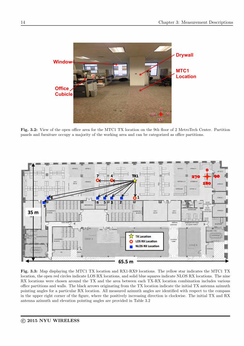
3.2 View of the open office area for the MTC1 TX location on the 9th floor of 2 MetroTech Center.Partition panels and furniture occupy a majority of the working area and can be categorizedas office partitions. . . . . . . . . . . . . . . . . . . . . . . . . . . . . . . . . . . . . . . . . . . 14
3.3 Map displaying the MTC1 TX location and RX1-RX9 locations. The yellow star indicates theMTC1 TX location, the open red circles indicate LOS RX locations, and solid blue squaresindicate NLOS RX locations. The nine RX locations were chosen around the TX and thearea between each TX-RX location combination includes various office partitions and walls.The black arrows originating from the TX location indicate the initial TX antenna azimuthpointing angles for a particular RX location. All measured azimuth angles are identified withrespect to the compass in the upper right corner of the figure, where the positively increasingdirection is clockwise. The initial TX and RX antenna azimuth and elevation pointing anglesare provided in Table 3.2 . . . . . . . . . . . . . . . . . . . . . . . . . . . . . . . . . . . . . . 14
3.4 View of the lobby area outside of two classrooms at the end of a long corridor for the MTC2TX location. . . . . . . . . . . . . . . . . . . . . . . . . . . . . . . . . . . . . . . . . . . . . . 15
3.5 Map displaying the MTC2 TX location, RX10 to RX22, and RX161 locations. The yellowstar indicates the MTC1 TX location, the open red circles indicate LOS RX locations, andsolid blue squares indicate NLOS RX locations. The 14 RX locations were chosen aroundthe TX and the area between each TX-RX link combination includes various obstructionsand partitions such as drywall, elevators, glass doors, and metal doors. RX16 and RX161are at the same location, but with the NYU WIRELESS front entrance glass door closedfor RX16, and open for RX161. The black arrows originating from the TX location indicatethe initial TX azimuth boresight angles for a particular RX location. All measured azimuthangles are identified with respect to the compass in the upper right corner of the figure, wherethe positively increasing direction is clockwise. The initial TX and RX antenna azimuth andelevation pointing angles are provided in Table 3.3. . . . . . . . . . . . . . . . . . . . . . . . . 16
3.6 View of the open room area with partition panels and office furniture obstructions near theMTC3 TX location. . . . . . . . . . . . . . . . . . . . . . . . . . . . . . . . . . . . . . . . . . 17
3.7 Map displaying the MTC3 TX location, RX16, RX17, and RX23-RX27 locations. The yellowstar indicates the MTC3 TX location, the open red circle indicates the LOS RX location, andthe solid blue squares indicate the NLOS RX locations. The seven RX locations were chosenaround the TX and are behind various combinations of walls, glass doors, and metal doors.The black arrows originating from the TX location indicate the initial TX antenna azimuthpointing angles for a particular RX location. All measured azimuth angles were identified withrespect to the compass in the upper right corner of the map, where the positively increasingdirection is clockwise. The initial TX and RX antenna azimuth and elevation pointing anglesare provided in Table 3.4. . . . . . . . . . . . . . . . . . . . . . . . . . . . . . . . . . . . . . . 18
3.8 View of the long corridor where the MTC4 TX was placed outside of the elevator partitionentrance. . . . . . . . . . . . . . . . . . . . . . . . . . . . . . . . . . . . . . . . . . . . . . . . . 19
ix
List of Figures
3.9 Map showing the MTC4 location and corresponding RX11-RX16, RX18, RX28, RX121, andRX161 locations. The yellow star indicates the MTC4 TX location, the open red circlesindicate the four LOS RX locations, and the solid blue squares indicate the six NLOS RXlocations. The black arrows originating from the TX location indicate the initial TX antennaazimuth pointing angles for a particular RX location. All azimuth angles in the measurementswere with respect to the compass in the upper right corner of the map, where the positivelyincreasing direction is clockwise. The initial TX and RX antenna azimuth and elevationpointing angles are provided in Table 3.5. . . . . . . . . . . . . . . . . . . . . . . . . . . . . . 19
3.10 View of the inside of the classroom where the MTC5 TX location was placed, surrounded bydesks and chairs. . . . . . . . . . . . . . . . . . . . . . . . . . . . . . . . . . . . . . . . . . . . 20
3.11 Map displaying the MTC5 TX location, and RX8, RX19, and RX28-RX33 locations. Theyellow star indicates the MTC5 TX location and the solid blue squares indicate the eightNLOS RX locations. The black arrows originating from the TX location indicate the initialTX antenna azimuth pointing angles for a particular RX location. All azimuth angles in themeasurements were with respect to the compass in the upper right corner of this figure, wherethe positively increasing direction is clockwise. The initial TX and RX antenna azimuth andelevation pointing angles are provided in Table 3.6. . . . . . . . . . . . . . . . . . . . . . . . . 21
3.12 Block diagram of the 28 GHz transmitter. The TX PN generator produced a 400 Mcps PNsequence that was modulated by a 5.4 GHz IF and then multiplied by a 22.6 GHz LO, thusupconverted to a 28 GHz centered RF signal. The RF signal was then transmitted through ahighly-directional horn antenna with 15 dBi of gain and 28.8◦ azimuth HPBW. . . . . . . . . 22
3.13 Block diagram of the 73 GHz transmitter. The TX PN generator produced a 400 Mcps PNsequence that was modulated by a 5.625 GHz IF and then multiplied by a 67.875 GHz (tripled22.625 GHz) LO, thus upconverted to a 73.5 GHz centered RF signal. The RF signal was thentransmitted through a highly-directional horn antenna with 20 dBi of gain and 15◦ azimuthHPBW. . . . . . . . . . . . . . . . . . . . . . . . . . . . . . . . . . . . . . . . . . . . . . . . . 23
3.14 Block diagram of the RX system used to characterize the 28 GHz indoor channel. The receivedsignal was downconverted from the 28 GHz centered RF signal via an LO of 22.6 GHz, whichwas then subsequently demodulated down to its I and Q baseband components via an IF-stage 5.4 GHz LO. A PN sequence identical to that at the TX was generated, but at a slightlyslower rate of 399.95 Mcps, and was then mixed with the received signal’s baseband I and Qsignals, that were used to recover a time-dilated impulse response of the channel. . . . . . . . 24
3.15 Block diagram of the RX system used to characterize the 73 GHz indoor channel. The receivedsignal was downconverted from the 73.5 GHz centered RF signal via an LO of 67.875 GHz,which was then subsequently demodulated down to its I and Q baseband components via anIF-stage 5.625 GHz LO. A PN sequence identical to that at the TX was generated, but at aslightly slower rate of 399.95 Mcps, and was then mixed with the received signal’s basebandI and Q signals, that were used to recover a time-dilated impulse response of the channel. . . 25
x

List of Tables
3.1 TX and corresponding RX locations measured for the 28 GHz and 73 GHz indoor propagationmeasurements referenced to Fig. 3.1. 3D T-R separation distance ranges are provided for eachTX and corresponding RX locations, as well as RX locations that experienced outage (e.g. nodetectable signal for all pointing angles) for V-V or V-H antenna polarization configurations.A “-” indicates no outage and the RX ID number indicates where an outage occurred. . . . . 12
3.2 TX and RX location IDs, T-R separation distances, initial TX and RX antenna azimuthand elevation pointing angles for each TX-RX location combination, and environment typesfor the co- and cross-polarization antenna configuration measurements for the MTC1 TXlocation. All angle configurations are the same for both 28 GHz and 73 GHz measurementsfor RX2-RX9. However, the RX1 initial angle configurations were different for the 28 GHzand 73 GHz measurements, as specified in the table. . . . . . . . . . . . . . . . . . . . . . . . 15
3.3 TX and RX location IDs, T-R separation distances, initial TX and RX antenna azimuth andelevation pointing angles for each TX-RX location combination, and environment types for theco- and cross-polarization antenna configuration measurements for the MTC2 TX location.All angle configurations are identical for the 28 GHz and 73 GHz measurements. . . . . . . . 16
3.4 TX and RX location IDs, T-R separation distances, initial TX and RX antenna azimuth andelevation pointing angles for each TX-RX location combination, and environment types for theco- and cross-polarization antenna configuration measurements for the MTC3 TX location.All angle configurations are identical for the 28 GHz and 73 GHz measurements. . . . . . . . 17
3.5 TX and RX location IDs, T-R separation distances, initial TX and RX antenna azimuth andelevation pointing angles for each TX-RX location combination, and environment types for theco- and cross-polarization antenna configuration measurements for the MTC4 TX location.All angle configurations are identical for the 28 GHz and 73 GHz measurements. . . . . . . . 20
3.6 TX and RX location IDs, T-R separation distances, initial TX and RX antenna azimuth andelevation pointing angles for the each TX-RX location combination, and environment typesfor the co- and cross-polarization antenna configuration measurements for the MTC5 TXlocation. All angle configurations are identical for the 28 GHz and 73 GHz measurements. . . 21
3.7 Broadband sliding correlator channel sounding system specifications for the 28 GHz and 73GHz indoor measurement campaign [6, 97–100]. . . . . . . . . . . . . . . . . . . . . . . . . . . 23
3.8 The measurement routine for each TX and RX location combination. Elevation angles arewith respect to boresight (initial) angles, which can be found in Tables 3.2 – 3.6. HPBWindicates the step increment in the azimuth plane (tilt change in the elevation plane), wherethe antenna azimuth HPBW for the 28 GHz measurements was 28.8◦, but the step incrementwas 30◦. As previously described the HPBW step increment for the 73 GHz measurementswas 15◦ . . . . . . . . . . . . . . . . . . . . . . . . . . . . . . . . . . . . . . . . . . . . . . . . 27
5.1 Path loss environment definitions for directional path loss models. . . . . . . . . . . . . . . . 33
xi
List of Tables
5.2 Single frequency directional CI path loss model (4.1) parameters with d0 = 1 m for 28 GHzand 73 GHz indoor channels with TX heights of 2.5 m and RX heights of 1.5 m for V-Vand V-H antenna polarization configurations. The 28 GHz TX and RX antennas had 15dBi (28.8◦ azimuth HPBW) of gain and the 73 GHz TX and RX antennas had 20 dBi (15◦
azimuth HPBW) of gain. “Freq.” stands for carrier frequency and “Pol.” stands for TX-RXantenna polarization configuration. The LOS distances ranged from 4.6 m to 21.3 m and theNLOS distances ranged from 3.9 m to 45.9 m. . . . . . . . . . . . . . . . . . . . . . . . . . . . 35
5.3 Single frequency directional CIX path loss model (4.2) parameters with d0 = 1 m for 28 GHzand 73 GHz indoor channels with TX heights of 2.5 m and RX heights of 1.5 m for V-Hantenna polarization configurations. The 28 GHz TX and RX antennas had 15 dBi (28.8◦
azimuth HPBW) of gain and the 73 GHz TX and RX antennas had 20 dBi (15◦ azimuthHPBW) of gain. “Freq.” stands for carrier frequency and “Pol.” stands for TX-RX antennapolarization configuration. . . . . . . . . . . . . . . . . . . . . . . . . . . . . . . . . . . . . . . 35
5.4 Single frequency directional FI path loss model (4.3) parameters for 28 GHz and 73 GHzindoor channels with TX heights of 2.5 m and RX heights of 1.5 m for both V-V and V-Hantenna polarization configurations. The 28 GHz TX-RX antennas had 15 dBi (28.8◦ azimuthHPBW) of gain and the 73 GHz TX-RX antennas had 20 dBi (15◦ azimuth HPBW) of gain.“Ant. Pol.” stands for antenna polarization. . . . . . . . . . . . . . . . . . . . . . . . . . . . . 35
5.5 28 GHz and 73 GHz multi-frequency directional path loss model parameters for the CI,CIX, CIF, CIFX, ABG, and ABGX models for LOS, NLOS, and NLOS-Best environmentsand scenarios. The CIX, CIFX, and ABGX cross-polarized models use the correspondingparameters found for their respective co-polarized models to find the XPD factor in dB thatminimizes σ. “Pol.” stands for polarization configuration (either V-V or V-H). . . . . . . . . 36
5.6 Path loss definitions for omnidirectional path loss models. . . . . . . . . . . . . . . . . . . . . 39
5.7 Single frequency omnidirectional CI path loss model parameters with d0 = 1 m and FI pathloss model parameters for 28 GHz and 73 GHz indoor propagation channels with TX heightsof 2.5 m and RX heights of 1.5 m for both V-V and V-H antenna polarization configurationsfor LOS and NLOS environments. “Freq.” stands for carrier frequency, “Pol.” stands forTX-RX antenna polarization configuration, and “Env.” stands environment. . . . . . . . . . . 41
5.8 Single frequency omnidirectional CIX path loss model parameters with d0 = 1 m for 28 GHzand 73 GHz indoor channels with TX heights of 2.5 m and RX heights of 1.5 m for V-Hantenna polarization configurations. The 28 GHz TX and RX antennas had 15 dBi (28.8◦
azimuth HPBW) of gain and the 73 GHz TX and RX antennas had 20 dBi (15◦ azimuthHPBW) of gain. “Freq.” stands for carrier frequency and “Pol.” stands for TX-RX antennapolarization configuration . . . . . . . . . . . . . . . . . . . . . . . . . . . . . . . . . . . . . . 41
5.9 28 GHz and 73 GHz multi-frequency omnidirectional path loss model parameters for the CI,CIX, CIF, CIFX, ABG, and ABGX models for LOS and NLOS environments. The CIX,CIFX, and ABGX cross-polarized models use the corresponding parameters found for theirrespective co-polarized models to find the XPD factor in dB that minimizes σ. “Pol.” standsfor polarization configuration (either V-V or V-H). . . . . . . . . . . . . . . . . . . . . . . . . 41
5.10 Single frequency combined polarization directional path loss models at 28 GHz and 73 GHzfor LOS, NLOS, and NLOS-Best scenarios. . . . . . . . . . . . . . . . . . . . . . . . . . . . . 43
5.11 28 GHz and 73 GHz multi-frequency combined polarization directional path loss models forLOS, NLOS, and NLOS-Best scenarios. . . . . . . . . . . . . . . . . . . . . . . . . . . . . . . 45
5.12 28 GHz and 73 GHz single frequency combined polarization CI and FI omnidirectional pathloss models for LOS and NLOS environments. . . . . . . . . . . . . . . . . . . . . . . . . . . . 45
5.13 28 GHz and 73 GHz multi-frequency combined polarization CI, CIF, and ABG omnidirectionalpath loss models for LOS and NLOS environments. . . . . . . . . . . . . . . . . . . . . . . . . 46
xii

List of Tables
6.1 Comparison of mean, standard deviation, and maximum RMS delay spreads at 28 GHz and73 GHz for V-V and V-H antenna polarization combinations in LOS and NLOS indoor prop-agation environments. “Ant. Pol.” means TX-RX antenna polarization and “Env.” indicatesthe environment type of the RX locations. . . . . . . . . . . . . . . . . . . . . . . . . . . . . . 53
6.2 Comparison of mean, standard deviation, and maximum RMS delay spreads at 28 GHz and 73GHz for combined antenna polarizations in LOS and NLOS indoor propagation environments.“Env.” indicates the environment type of the RX locations. . . . . . . . . . . . . . . . . . . . 53
B.1 28 GHz co-polarized antenna (V-V) omnidirectional path loss values with corresponding En-vironment (Env.) TX IDs, RX IDs, path loss (PL) in dB, and 3D T-R separation distance inmeters. . . . . . . . . . . . . . . . . . . . . . . . . . . . . . . . . . . . . . . . . . . . . . . . . . 70
B.2 28 GHz cross-polarized antenna (V-H) omnidirectional path loss values with correspondingEnvironment (Env.) TX IDs, RX IDs, path loss (PL) in dB, and 3D T-R separation distancein meters. . . . . . . . . . . . . . . . . . . . . . . . . . . . . . . . . . . . . . . . . . . . . . . . 71
B.3 73 GHz co-polarized antenna (V-V) omnidirectional path loss values with corresponding En-vironment (Env.) TX IDs, RX IDs, path loss (PL) in dB, and 3D T-R separation distance inmeters. . . . . . . . . . . . . . . . . . . . . . . . . . . . . . . . . . . . . . . . . . . . . . . . . . 72
B.4 73 GHz cross-polarized antenna (V-H) omnidirectional path loss values with correspondingEnvironment (Env.) TX IDs, RX IDs, path loss (PL) in dB, and 3D T-R separation distancein meters. . . . . . . . . . . . . . . . . . . . . . . . . . . . . . . . . . . . . . . . . . . . . . . . 73
C.1 Single frequency directional path loss model standard deviations for the CI model with d0 = 1m, the CIX model, and the FI path loss model. “Freq.” stands for carrier frequency, “Pol.”stands for TX-RX antenna polarization configuration, “Env.” stands for environment, and“Comb.” stands for combined polarization. Differences in standard deviations are also shown. 75
C.2 Multi-frequency directional path loss model standard deviations for the CI, CIX, CIF, CIFX,ABG, and ABGX large-scale path loss models. “Pol.” stands for TX-RX antenna polarizationconfiguration, “Env.” stands for environment, and “Comb.” stands for combined polarization.Differences in standard deviations are also shown. . . . . . . . . . . . . . . . . . . . . . . . . 76
C.3 Single frequency omnidirectional path loss model standard deviations for the CI model withd0 = 1 m, the CIX model, and the FI path loss model. “Freq.” stands for carrier frequency,“Pol.” stands for TX-RX antenna polarization configuration, “Env.” stands for environment,and “Comb.” stands for combined polarization. Differences in standard deviations are alsoshown. . . . . . . . . . . . . . . . . . . . . . . . . . . . . . . . . . . . . . . . . . . . . . . . . 76
C.4 Multi-frequency omnidirectional path loss model standard deviations for the CI, CIX, CIF,CIFX, ABG, and ABGX large-scale path loss models. “Pol.” stands for TX-RX antennapolarization configuration, “Env.” stands for environment, and “Comb.” stands for combinedpolarization. Differences in standard deviations are also shown. . . . . . . . . . . . . . . . . 77
xiii

This page is intentionally left blank.

Chapter 1
Introduction
1.1 Millimeter-Wave Communications Background and Motivation
Over the past few years there has been an explosion in mobile data traffic as a consequence of the growthof smartphones, tablets, and devices that provide, monitor, transfer, and record ZettaBytes of data everyyear [1–3]. Smartphone adoption rates are sharply increasing as carriers and service providers attempt toattract more customers [4, 5]. The advent of smartphones and “Wireless Fidelity” (WiFi) enabled deviceshas facilitated the surge in wireless technologies and applications, but has created congestion in the sub–6GHz spectrum in which a majority of these devices operate in [6–9].
The 2.4 GHz and 5 GHz WiFi bands have been widely used for indoor wireless communications in typicaloffice environments, restaurants, and hotels since the early 2000’s [10, 11], but dense deployment of indoorhotspots and new wireless multimedia devices has led to increased congestion and traffic over indoor net-works [12]. Offices are “cutting the cord,” by investing in numerous wireless multimedia devices for video.In addition to the 2.4 GHz and 5 GHz WiFi bands, the 60 GHz millimeter-wave (mmWave) band is usedfor WiGig to support high-data-rate applications. The vast available bandwidth (57-64 GHz) at 60 GHz(and unlicensed availability in the U.S. and other countries) motivated extensive 60 GHz indoor propaga-tion measurements to understand channel characteristics necessary for designing indoor wireless local areanetwork (WLAN) systems capable of achieving multi-gigabits-per-second throughputs [13, 14]. The study ofmmWave propagation has been widely conducted at 60 GHz (with fewer studies at other mmWave bands)for common indoor environments in order to properly model path loss and channel characteristics.
The impending spectrum and capacity crunch for outdoor cellular may very well lead to the use of the 28GHz and 73 GHz mmWave frequency bands as an extension for 5G outdoor and indoor communications,especially due to the trend of shrinking cell sizes. If the 28 GHz and 73 GHz bands are to eventually becomeunlicensed similar to the 60 GHz band, the wide range of applications and events they could support wouldtremendously reduce the load on the cellular and backhaul networks as we move into the age of Internetof Things (IoT) [15]. In any case, extensive indoor propagation measurements at the 28 GHz and 73 GHzbands are needed in order to accurately characterize and model the channel to design capable indoor systemsat these frequencies.
1.2 Project Overview
The NYU WIRELESS research center conducted extensive measurements at 28 GHz and 73 GHz withvarious transmitter (TX) and receiver (RX) antenna azimuth and elevation pointing angle combinations and

2 Chapter 1: Introduction
for different antenna polarization configurations in the summer of 2014 in a typical office building. Over 70GB of raw data were collected and are the basis for the models and characteristics presented in this report.
The measurements were conducted on the 9th floor of 2 MetroTech Center (MTC) in Downtown Brooklyn,New York. The single floor office environment (35 meters × 65.5 meters) consisted of typical office partitionsand furniture (such as cubicles, desks, chairs, metal shelves, wood closets, concrete walls, glass doors,and elevator doors). A 400 Megachips-per-second (Mcps) sliding correlator channel sounding system andtwo pairs of steerable directional horn antennas were used to measure co- and cross-polarization channelcharacteristics at the 28 GHz and 73 GHz frequency bands. A pair of 15 dBi gain horn antennas with 28.8◦
half-power beamwidth (HPBW) in the azimuth plane and a pair of 20 dBi gain horn antennas with 15◦
HPBW in the azimuth plane were used at the TX and RX when performing measurements at 28 GHz and73 GHz, respectively. Five TX locations and 33 RX locations with 48 overall TX-RX location combinationsand with transmitter-receiver (T-R) separation distances ranging from 3.9 meters (m) to 45.9 m were chosenin order to investigate the complex indoor propagation channels. The TX antennas were set at heights of2.5 m (near the ceiling) above ground level (AGL) to emulate indoor wireless access points, and the RXantennas were fixed at heights of 1.5 m AGL (similar to the height of a mobile phone carried by a human).For each measured TX-RX location combination, 16 different unique pointing angle measurement sweepswere performed to investigate angle of departure (AOD) and angle of arrival (AOA) statistics, and a powerdelay profile (PDP) was acquired at each unique azimuth and elevation antenna pointing angle, separatedby step increments of 15◦ or 30◦ in the azimuth plane for the 28 GHz and 73 GHz frequencies, respectively.The measurements included two antenna polarization combinations: vertical-to-vertical (V-V), where theTX and RX antennas were vertically polarized (perpendicular to the ground), and vertical-to-horizontal(V-H), where the TX antenna was vertically polarized and the RX antenna was horizontally polarized, inorder to study the impact of polarization for indoor mmWave communications systems at 28 GHz and 73GHz.
1.3 Report Overview
The following sections of the report discuss details from numerous indoor propagation campaigns below 6GHz and above 6 GHz in the mmWave frequency bands including measurement hardware, environments,configurations, and results. The specifications regarding the 28 GHz and 73 GHz measurement equipmentthat was used to measure the indoor channel at NYU are also described, in addition to the measurementprocedures, settings, and scenarios for all 48 TX-RX location combinations conducted at each band. Tradi-tional single frequency path loss models such as the close-in free space reference distance (CI) and alpha-betafloating-intercept (FI) models are discussed, in addition to multi-frequency path loss models such as thealpha-beta-gamma (ABG) model and a new close-in free space reference distance with frequency weightingfactor (CIF) model. Furthermore, cross-polarized versions of each path loss model, that includes a cross-polarization discrimination (XDP) factor are introduced. The closed-form expressions for optimizing modelparameters are provided in Appendix A. After introducing the models, the report gives the estimated di-rectional and omnidirectional path loss model parameters for separate and combined polarizations for singleand multi-frequency path loss models from line-of-sight (LOS) and non-line-of-sight (NLOS) measurementdata. Multipath time dispersive characteristics from the directional measurements are then provided for thebest and worst cases (smallest and largest delay spreads), and for the unique pointing angles that resulted inthe lowest path loss between the TX and RX for each location combination. Time dispersive characteristicsare given for both separate and combined polarization scenarios.
c© 2015 NYU WIRELESS

Chapter 1: Introduction 3
In Appendix B a compilation of the post-processed omnidirectional path loss data at 28 GHz and 73 GHzis provided so that researchers may generate their own omnidirectional path loss models and perform anal-yses from the measurement data. As previously mentioned, the closed-form expressions that optimize theparameters for each model are given in Appendix A.
c© 2015 NYU WIRELESS

This page is intentionally left blank.
Chapter 2
Literature Review
This chapter presents an extensive literature review on previous indoor propagation studies that have focusedon wireless channel characterization for the creation of statistical models, vital to the development of newstandards and technologies for wireless communications systems. The current WiFi and 4G standards weredeveloped based on propagation measurements that assisted in accurately characterizing the temporal andspatial indoor propagation channel below 6 GHz frequencies. A literature review of channel measurementsand models is presented for frequencies below 6 GHz and above 6 GHz (mainly focused on 60 GHz) forvarious indoor scenarios.
2.1 Below 6 GHz
Extensive studies for indoor wireless propagation and channel models below 6 GHz have been conducted formany years. As just a sample of typical work in an indoor office environment, a 900 MHz signal with 200kHz of bandwidth experienced between 28 and 61 dB of attenuation per decade of distance for distances upto 27 m, across multiple floors [16]. Ericsson used a path loss model from multi-floor measurements of anoffice building that had four breakpoints, but assumed 30 dB of attenuation at d0 = 1 m (free space for firstmeter) at 900 MHz and measured a PLE of 2 for up to 10 m, and used a multiple slope model at greaterdistances [17]. Indoor multipath propagation measurements were performed by Saleh and Valenzuela with a10 ns probing pulse centered at 1.5 GHz with vertically polarized discone TX and RX antennas at 2 meter(m) heights [18]. The indoor channel was observed to vary slowly with time, resulting in maximum RMSdelay spreads of 50 ns in adjacent rooms, and signal attenuation between 30 dB and 40 dB per decade ofdistance.
Bultitude measured the 910 MHz band in an indoor office-style building with a CW (continuous wave) tonetransmitted at 500 mW with an omnidirectional TX antenna, and a quarter-wave monopole RX antenna [19].Results indicated that in line-of-sight (LOS) environments, signal attenuation over distance closely followedFriis’ free space path loss equation where propagating signals attenuate following the square power law. Insome cases, the received power was greater than predicted free space propagation, indicating a waveguideeffect in narrow hallways of the office building.
In the late 1980’s, Motley and Keenan performed indoor multi-floor measurements and found PLEs of 4 and3.5 relative to a 1 m free space reference distance at 900 MHz and 1700 MHz, respectively, using TX andRX dipole antennas [20]. Rappaport et al. conducted wideband multipath measurements at 1300 MHz infactory buildings with a 10 nanosecond (ns) transmitting pulse in both LOS and NLOS environments with

6 Chapter 2: Literature Review
TX and RX discone antennas that resulted in path loss attenuation of 22 dB per decade of distance and anRMS delay spread that ranged from 30 ns to 300 ns [21].
In the early 1990’s, Rappaport et al. performed indoor measurements at 1.3 GHz and 4.0 GHz for bothcircularly and linearly polarized antennas. Results indicated similar propagation path loss for both fre-quencies, and larger cross-polarization discrimination was found in LOS channels compared to NLOS orobstructed channels [22–24]. Additionally, the use of an omnidirectional TX antenna and a directionalcircularly-polarized RX antenna provided the lowest RMS delay spread and the lowest maximum excessdelay (10 dB down) compared to various polarizations of omnidirectional and directional antennas.
A paper on indoor propagation by J. B. Andersen et al. in 1995 highlighted the value of using a 1 m close-infree space reference distance for meaningful indoor path loss models [25]. The paper also demonstrated theviability of ray-tracing for indoor channel impulse response prediction for single and multi-floor propagation.Single story retail and grocery stores had PLEs of 2.2 and 1.8 at 914 MHz, respectively, with respect to(w.r.t.) a 1 m reference distance. Indoor offices with soft partitions measured at 900 and 1900 MHz hadPLEs w.r.t. a 1 m reference distance of 2.4 and 2.6, respectively, with standard deviations between 9.6dB and 14.1 dB. Radio-frequency penetration was also reported to attenuate between 3 dB and 30 dB formetallic tinted windows. Rappaport and Sandhu published a survey paper in 1994 that summarized radio-propagation measurements for frequencies between 850 MHz and 4000 MHz and the problems of radio-wavepropagation into buildings for wireless communications systems [26]. Average floor attenuation factors werefound to be 24.4 dB and 31.6 dB at 914 MHz for a transmitter and receiver separated by 3 floors in twodifferent office buildings.
Alvarez et al. studied the indoor radio channel between 1 GHz and 9 GHz, and defined four scenarios: LOS(when there was a direct path between the TX and RX), Soft-NLOS (when there was no direct path, butrather reflected paths between the TX and RX), Hard-NLOS (when there was no direct or reflected pathbetween the TX and RX), and corridor (special case for LOS, when there was a direct path and many strongreflected paths between the TX and RX) [27]. A VNA channel sounder with omnidirectional TX and RXantennas was used to record the channel transfer function by concatenating frequency sweeps between 1 and5 GHz and 5 and 9 GHz. The estimated PLEs from the measurement data were 1.4 (d0 = 15.1 cm) for theLOS scenario, 3.2 (d0 = 8.2 cm) for Soft-NLOS, and 4.1 (d0 = 6.7 cm) for Hard-NLOS.
Ghassemzadeh et al. used a Vector Network Analyzer (VNA) to transmit an ultra-wideband 1250 MHzradio-frequency (RF) bandwidth signal centered at 5 GHz with a conical monopole omnidirectional TX andRX antenna inside 23 homes in northern and central New Jersey [28]. In LOS environments the close-in freespace reference distance path loss model relative to a 1 m free space path loss (FSPL) distance resulted in aPLE of 1.7, and was determined to be 3.1 in NLOS environments. The standard deviation or shadow factorabout the mean path loss lines ranged from 2.8 dB to 4.4 dB, indicating small large-scale signal fluctuationsin the indoor home environments for ultra-wideband propagation at 5 GHz.
In the late 1990’s Durgin et al. performed numerous CW indoor and outdoor-to-indoor measurementsbetween walls and other partitions to derive path loss models in residential areas at 5.85 GHz [29–32]. Thepropagation models developed from the measurements were helpful for outdoor-to-indoor deployments, asthe main results indicated that signals that penetrated homes attenuated on average by about 14 dB, withtree shadowing attenuation that varied from 11 dB to 16 dB. Close-in building shadowing also attenuatedthe propagating signals by 15 dB to 21 dB, depending on RX antenna heights.
Durgin et al. studied angle delay and dispersion characteristics for outdoor and indoor peer-to-peer channelscentered at 1920 MHz in the early 2000’s. Both omnidirectional and directional (30◦ half-power beamwidth(HPBW)) antennas were used to measure angles of arrival and delay spread statistics. Typical results foroutdoor cross-campus measurements resulted in 17 ns to 219 ns RMS delay spreads, whereas three indoor-to-indoor locations resulted in 27 ns to 34 ns RMS delay spreads and 0.73-0.90 angular spreads [33, 34].
c© 2015 NYU WIRELESS
Chapter 2: Literature Review 7
Patawari et al. also studied peer-to-peer propagation, but at 1.8 GHz with low antenna heights and with200 MHz of first null-to-null RF bandwidth, with measured RMS delay spreads up to 330 ns in rural areasand up to 200 ns in urban peer-to-peer environments [35].
Ray-tracing simulations are another popular method for modeling indoor and outdoor propagation channels,and are less time-intensive and less costly compared to actual measurements. Motorola demonstrated theviability of ray-tracing for its revolutionary 18 GHz Altair WLAN product in the early 1990’s [36]. TheUniversity of Bristol and Virginia Tech were two of the first institutions to demonstrate the promise ofray-tracing for small-cell and indoor deployments [37]. Schaubach et al. used geometric optics to estimateaverage path loss and delay spread in microcellular environments by building database environments andwriting a computer program to perform ray-tracing on the databases. Simulations compared with time-delaymeasurements at 914 MHz on the Virginia Tech campus validated the program and methodology [38].
Work by Seidel et al. in the 1990’s showed good agreement for path loss and delay spread characteristicsusing predictive ray-tracing techniques and measurements at 1.3 GHz and 4.0 GHz. The predicted andmeasured path loss differed by less than 6 dB over most locations and RMS delay spreads were within 20 nsfor each measured location in rooms with 4.5 m ceiling heights [39, 40]. Additional ray-tracing simulationsusing 3D building databases and transmitted, reflected, and scattered ray mechanisms successfully predictedpropagation at 1900 MHz using a spread spectrum system [41]. An indoor ray-tracing software developed inthe 1990’s was able to predict path loss, partition loss, and floor attenuation loss for indoor environments atvarious sub-6 GHz frequencies by taking advantage of attenuation models based on the types of partitions,frequency, and distance [42, 43]. Improved ray-tracers for indoor wireless propagation included 3D ray-launching methods by using geodesic spheres and distributed wavefronts to increase accuracy and predictionat 900 MHz [44].
A measurement-based statistical indoor radio-channel impulse response model (SIRCIM) and statisticaloutdoor simulator (SMRCIM) were successfully implemented from many thousands of collected channelimpulse responses (CIRs) in factories at 1.3 GHz [45, 46], and from outdoor cellular channel PDPs [47, 48].These CIR models were popular with industry in the 1990’s during the early years of digital cellular andWiFi [49]. The SIRCIM and SMRCIM models were based on statistical and geometrical models to synthesizethe phases and directions of arrival and departure in an IR model [49, 50].
2.2 Above 6 GHz
Many studies at mmWave bands for the indoor environment have been conducted, predominantly in the 60GHz band, one of the most promising candidates for multi-gigabit wireless indoor communications systems.The large swath of available spectrum in the unlicensed 57-66 GHz band (60 GHz band) represents one ofthe largest unlicensed areas of spectrum real-estate to achieve ultra-high data rates for multi-Gbps wirelesscommunications performance, spectrum flexibility, and capacity [51, 52]. While the 60 GHz spectrum hasa large amount of bandwidth to offer, oxygen attenuation is more severe than other mmWave bands [53].Yong et al. presented an overview of 60 GHz technologies and their potential to provide next generationmulti-gigabit wireless communications, along with a series of technical challenges to resolve before large-scaledeployments [54]. Today, higher transmit power is allowed at 60 GHz compared to other existing wirelesslocal area networks (WLANs) and wireless personal area network (WPANs) systems. While high path lossin the first meter of propagation and transmission loss at 60 GHz may limit the operation to one room,interference is reduced compared to the severe interference experienced in the congested 2-2.5 GHz and 5-5.8GHz bands. Additionally, the form factor of mmWave systems and antennas will be smaller, comparedto sub-6 GHz systems, making it convenient highly-directional steerable antenna arrays to be integratedinto electronic products [55–57]. A number of open issues and technical challenges have yet to be fully
c© 2015 NYU WIRELESS

8 Chapter 2: Literature Review
addressed at 60 GHz, and they can be generally classified into the following categories: channel propagation,antenna technologies, RF solutions, and modulation schemes [54, 58–61]. Next-generation WLANs will alsoexploit 60 GHz spectrum with the development of the IEEE 802.11ad and WiGig standards, supported byWiFi companies who recognized that current spectral resources are insufficient for next-generation applica-tions [51, 53]. Researchers in Japan conducted pioneering research in the 1990’s in the 60 GHz band, anddeveloped point-to-point base-stations and user-stations with mmWave monolithic microwave integrated cir-cuit (MMIC) devices with antennas the size of a quarter that could transmit as high as 156 Mbps for wirelesslocal area networks (WLANs) [62, 63]. In a recent indoor experiment down a narrow hallway, researcherswere able to transmit 7.5 Gbps at a distance of 15 m using a high gain Antipodal Linear Tapered SlotAntenna (ALTSA) at 60 GHz [64], with additional studies resulting in path loss exponents slightly abovefree space (n = 2) in LOS [65]. Researchers in India also focused on mmWave antenna design at 60 GHzwith relatively high gains and small form factors for gigabit wireless communications and applications [66].
There have been extensive channel measurements and modeling efforts for indoor and outdoor scenarios at 60GHz, but this report focuses on indoor environments. Some of the earliest mmWave indoor channel modelingwork happened in Europe and Japan. Smulders et al. performed frequency-domain measurements across2 GHz of bandwidth centered at 58 GHz in an indoor environment and employed biconical horn antennaswith omnidirectional radiation patterns at the TX and RX [67–69]. The wideband mmWave measurementsyielded RMS delay spreads between 15 ns and 45 ns in small rooms and between 30 ns and 70 ns in largerrooms indicating that more paths with considerable energy arrive at the receiver over a larger time delay inlarger rooms. A worst case RMS delay spread of 100 ns was also reported.
Xu et al. studied the 60 GHz indoor channel using a directional horn antenna with 7◦ HPBW in the azimuthplane and 29 dBi of gain at the RX, and an open-ended waveguide with 90◦ HPBW in the azimuth plane and6.7 dBi of gain at the TX [13, 70]. A sliding correlator channel sounder was utilized with an RF null-to-nullbandwidth of 200 MHz and a 10 ns time resolution, with power delay profiles (PDPs) or channel impulseresponses, captured at discrete pointing angles while rotating the RX antenna. LOS measurements resultedin a PLE less than 2 (theoretical FSPL), relative to a 1 m close-in free space reference distance. Thesefindings were similar to those at lower frequencies in indoor environments, where ground and ceiling bouncereflections and a waveguide effect are known to increase power at the receiver such that the measured pathloss is less than theoretical FSPL.
Measurements similar to those conducted by Xu et al., were performed by Bensebti et al. to study large-scalepath loss in the indoor multipath propagation channel at 60 GHz at the University of Bristol using a spreadspectrum channel sounder with directional, semi-directional, and omnidirectional TX and RX antennasplaced at heights of 1.5 m [71]. Excess delay spreads ranged from 10 ns to 40 ns over short distances, withminimal deep fades. The total received discrete power was exponentially distributed in a LOS environmentalong a corridor that was 3 m x 30 m for 7 m to 33 m transmitter-receiver (T-R) separation distances.
Zwick et al. performed numerous wideband channel measurements at 60 GHz using a heterodyne transmitterand receiver. They measured propagation at 60 GHz with a channel sounder consisting of a 500 MHzbandwidth (2 ns resolution) PN sequence as the probing signal that was transmitted at 10 different frequencyslots between 59 GHz and 64 GHz and concatenated the measurements (for 5 GHz of total bandwidth), usingomnidirectional antennas in several different rooms for short-range distances [72]. Using omnidirectional TXand RX antennas, they measured median RMS delay spreads from 3 ns to 9 ns, in addition to calculatinga PLE of 1.33 relative to a 1 m free space reference distance and a shadow factor of 5.1 dB across allmeasurements.
Geng et al. conducted 60 GHz propagation measurements in various indoor environments in continuous-route (CR) and direction-of-arrival (DOA) measurement campaigns [73]. The RMS delay spread trended toa log-normal distribution, and the typical range was from 3 ns to 80 ns. The propagation mechanisms werestudied based on DOA measurements, indicating that the direct wave and the first-order reflected waves
c© 2015 NYU WIRELESS
Chapter 2: Literature Review 9
from smooth surfaces were sufficient in LOS propagation environments, while in NLOS cases, diffraction wasa significant propagation mechanism, and the transmission loss through walls was very high. Geng et al.also conducted 60 GHz measurements in corridor, LOS hallway, and NLOS hallway environments, and themeasured PLEs were 1.6 in LOS corridor, 2.2 in LOS hallway, and 3.0 in NLOS hallway environments [74].
Anderson et al. conducted indoor wideband measurements at 2.5 GHz and 60 GHz using a broadbandvector sliding correlator channel sounder to record PDPs [75, 76]. For the 2.5 GHz measurements, both thetransmitter and receiver antennas were vertically polarized omnidirectional biconical antennas with 6 dBiof gain. The transmit power before the antenna was 0 dBm in order to emulate the same operating powerof 2.4 GHz WLAN networks. For the 60 GHz measurements, vertically polarized pyramidal horn antennaswith 25 dBi of gain and a HPBW of 50◦ were used at both the transmitter and receiver. The transmit powerwas -10 dBm in order to maintain the linear operation of the power amplifier at the transmitter and to avoidsaturating the low noise amplifier of the receiver at short distances. An EIRP of 15 dBm was comparable tothe power of a femtocellular system to study a typical single-cell-per-room network environment. Anderson etal. selected eight transmitter locations and 22 receiver locations with T-R separation distances from 3.5 m to27.4 m on the same floor in a modern office building with a variety of obstructions in the signal path [75, 76].The transmitter and receiver locations were chosen to represent a wide range of typical office femtocellularpropagation environments. The heights of the transmitter and receiver antennas were 1.2 m relative to theground, with an exception at one receiver location where the RX antenna was 2.4 meters relative to the floor.By using a minimum mean square error fit, the PLE with respect to a 1 m free space reference distance at2.5 GHz was found to be 2.4 with a standard deviation of 5.8 dB, and at 60 GHz the PLE was 2.1 with astandard deviation of 7.9 dB.
Manabe et al. investigated how the radiation patterns and antenna polarizations at remote terminals affectsmultipath propagation characteristics at 60 GHz, in a conference room [77, 78]. Four types of antennaswere used to examine the effects of radiation patterns of RX antennas: an omnidirectional antenna andthree directive antennas with wide, medium, and narrow HPBWs. The use of a directive antenna at theremote terminal was an effective method to reduce the effects of multipath propagation. Further reductionin multipath effects was achieved with the use of circularly polarized directive antennas instead of linearlypolarized directive antennas.
In 2005, Moraitis and Constantinou performed indoor 60 GHz radio channel measurements by recordingpower delay profiles using a direct RF pulse technique with a 10 ns repetitive square pulse, modulated up tothe 60 GHz carrier having a bandwidth of 100 MHz and 10 dBm of transmit power while using identical 21dBi vertically polarized horn antennas at the TX and RX [79]. The extracted power delay profiles revealedthat excess delay was much less in hallways (up to 8.18 ns) compared to offices (up to 14.69 ns). Themeasurements also revealed that the office environment did not experience large channel variation over localareas.
Maltsev et al. used an 800 MHz OFDM channel sounder centered at 60 GHz using circular horn antennasat the transmitter and receiver and found that cross-polarized antennas in LOS environments could yieldapproximately 20 dB of isolation at 60 GHz [14, 80], and about 10-20 dB of isolation for NLOS environments.Torkildson et al. investigated the potential for exploiting spatial multiplexing as a means to increase spectralefficiency at 60 GHz in an indoor environment [81, 82]. The robustness of a link was observed to improve byincreasing the number of antennas at the RX, which would also reduce the sensitivity of the channel capacity.The indoor channel was significantly degraded when the LOS path was blocked due to an obstruction,suggesting more accurate and elaborate channel models were needed to better assess link performance inthe absence of a LOS path.
Aside from the majority of indoor propagation research at 60 GHz, little is known about other mmWavebands. In the early 1990’s, Motorola conducted extensive 18 GHz indoor propagation measurements us-ing both sectored and omnidirectional antennas in support of their Altair WLAN product, but little was
c© 2015 NYU WIRELESS
10 Chapter 2: Literature Review
published. Haneda et al. conducted numerous measurement campaigns in the 60 GHz and 70 GHz bandsin indoor shopping malls, railway stations, and office environments using a VNA based channel soundingmethod over 5 GHz of bandwidth [83, 84]. The measurements employed a directional horn antenna at theTX with 20 dBi of gain, and a biconical omnidirectional antenna at the RX. Specular reflections in the prop-agation channel accounted for 75% of the received power in office environments, and 90% of the receivedpower in a shopping mall and railway station, and delay spreads were similar at both 60 GHz and 70 GHz.
Wu et al. conducted 28 GHz indoor laboratory measurements using horn antennas that rotated in the entireazimuth plane while using a VNA to measure the channel [85]. They used the Saleh-Valenzuela model tocharacterize the indoor channel and were able to extract intra-cluster parameters. Lei et al. also performedindoor 28 GHz channel propagation measurements in an indoor environment with a VNA and a pair of 26dBi gain horn antennas for distances up to 30 m. Path loss attenuation slopes as a function of log-distancein different indoor environments were estimated to be 2 in free space, 2.2 in a hallway, 1.2 in a corridor, and1.8 in an office [86].
2.3 Recent Activities for Indoor MmWave Studies
Research groups are now beginning to study the indoor propagation channel at mmWave frequencies otherthan 60 GHz. Fixed point-to-point WLANs in the 71–76 GHz, 81–86 GHz, and 92–95 GHz bands have been,or soon will be deployed using light licensing rules and recommendations by the Federal CommunicationsCommission (FCC) [87, 88] in the United States, the Electronic Communications Commission (ECC) [89] inEurope, the Office of Commission (Ofcom) [90] in the United Kingdom, the Canadian Radio-television andTelecommunications Commission (CRTC) [91] in Canada, and the Australian Communications and MediaAuthority (ACMA) [91] in Australia.
An even stronger indication for the impending use of mmWave frequency bands in future fifth generation(5G) indoor and outdoor wireless communications systems can be found in public comments filed in responseto the FCC’s 2014 notice of inquiry (NOI) FCC 14-154 and FCC 14-177 regarding the use of spectrum above24 GHz [92, 93]. The UK Office of Commission (Ofcom) requested similar public comments in 2015 on theuse of spectrum in higher mmWave frequency bands [94]. It is also noted here that mmWave frequencies areused for other applications and have a wide range of use cases, specifically passive imaging which is becomingmore widespread as a means for detecting concealed weapons and for through-the-wall imaging [95].
c© 2015 NYU WIRELESS
Chapter 3
Measurement Descriptions
Measurements were conducted in the NYU WIRELESS research center on the 9th floor of 2 MetroTech Centerin Downtown Brooklyn, New York, which is a 10-story building constructed in the early 1990’s with tintedwindows and steel reinforcement between each floor. The 9th floor is a typical single floor office environmentwith common obstructions such as desks, chairs, cubicle partitions, offices, classrooms, doors, hallways, wallsmade of drywall, and elevators. We tried to measure between adjacent floors (9th to 10th) with a wide rangeof antenna pointing angle combinations between the TX and RX at 73 GHz with maximum transmit power,but the metal and concrete structure and tinted glass windows of the building prevented any signals frombeing measured between adjacent office floors. This test was not attempted at 28 GHz. Identical TX andRX locations were used for both the 28 GHz and 73 GHz measurements with both co- and cross-polarizationantenna configurations between the TX and RX. For co-polarization measurements, the TX and RX hornantennas were vertically polarized (V-V), whereas for the cross-polarization measurements, the TX antennawas vertically polarized and the RX antenna was horizontally polarized (V-H). Since future mmWave wirelesssystems will be used by people and appliances with various physical orientations, approximately half of themeasurements used co-polarized antennas at the TX and RX, and half used cross-polarized antennas. TXantennas were placed 2.5 m above the floor, very close to the 2.7 m ceiling to emulate common indoorhotspot locations, and RX antennas were placed 1.5 m above the floor (typical handset level heights).
3.1 Locations and Environments
Five TX locations and 33 RX locations were selected, resulting in measurements from 48 TX-RX locationcombinations that had 3D transmitter-receiver (T-R) separation distances ranging from 3.9 m to 45.9 m,with RX locations chosen in LOS and NLOS environments (the floor dimensions were 35 m x 65.5 m).The 10 LOS measurement locations had 3D distances ranging from 4.6 m to 21.3 m, and the 38 NLOSmeasurement locations had 3D distances that ranged from 3.9 m to 45.9 m.
Fig. 3.1 displays a map of the five TX locations, the 33 RX locations (some were used for multiple transmit-ters), and basic descriptions of the surrounding obstructions. The 33 RX locations were randomly chosenaround the corresponding TX locations with various combinations of partition materials between the TXsand RXs. The height of the office floor walls (drywall) was approximately 2.7 m, and most doors had heightsof 2.1 m relative to the floor. Each TX was set to 2.5 m AGL (close to the ceiling), while each RX was setto 1.5 m AGL (just below cubicle partition heights of 1.7 m). The measurement environment was a closed-plan in-building scenario that included line-of-sight and non-line-of-sight corridor, hallway, cubicle-farm,and adjacent-room communication links. A corridor environment is when a propagating signal travels downa corridor to reach the receiver by a line-of-sight path, reflections, scattering, and/or diffraction, but not

12 Chapter 3: Measurement Descriptions
Table 3.1: TX and corresponding RX locations measured for the 28 GHz and 73 GHz indoor propagation measure-ments referenced to Fig. 3.1. 3D T-R separation distance ranges are provided for each TX and corresponding RXlocations, as well as RX locations that experienced outage (e.g. no detectable signal for all pointing angles) for V-V orV-H antenna polarization configurations. A “-” indicates no outage and the RX ID number indicates where an outageoccurred.
TX ID RX IDs T-R Dist (m)V-V V-H
Outages Outages28 GHz 73 GHz 28 GHz 73 GHz
1 1–9 6.4 ≤ d ≤ 32.9 - 9 9 8, 9
2 10, 11–22, 161 4.1 ≤ d ≤ 45.9 - 17, 20 14, 15, 17 13–15, 17, 19, 20
3 16,17, 23–27 5.3 ≤ d ≤ 8.7 - - - -
4 11–16, 18, 28, 121, 161 7.1 ≤ d ≤ 33.0 - - - -
5 8, 19, 28–33 3.9 ≤ d ≤ 31.2 - - - -
penetration. An open-plan environment includes a cubicle-farm and a central TX location around soft parti-tions such as cubicle walls [43, 96]. A closed-plan environment is when a propagating signal must penetratean obstruction such as a fixed building wall to reach the receiver. All of these measurement environmentstypically occur in a closed-plan indoor environment.
A subset of RX locations (typically 8 to 10) were measured for each TX location during the measurementcampaign. The identical 48 TX-RX location combinations were measured at 28 GHz and 73 GHz, to enabledirect comparison across the two frequency bands. Table 3.1 provides the RX locations that were measuredfor each TX location, and indicates which TX-RX combinations resulted in outages (for V-V, V-H, or bothantenna polarization configurations).
Fig. 3.1: Map of the 2 MetroTech Center 9th floor with five TX locations and 33 RX locations. The yellow starsrepresent the TX locations, and the red dots represent the RX locations.
c© 2015 NYU WIRELESS

Chapter 3: Measurement Descriptions 13
Measured environment types were categorized according to the following definitions for each unique antennapointing angle in the azimuth and elevation planes between the TX and RX antennas:
• Line-of-Sight Boresight (LOS B): when both the TX and RX antennas are pointed directly towardseach other on boresight and aligned in both the azimuth and elevation planes with no obstructionsbetween the antennas. For LOS environments, only the first rotation index (Rot 0)∗ of Measure-ment 1 and Measurement 9 (RX sweeps), and of Measurement 6 and Measurement 14 (TXsweeps) were considered LOS B measurements since the Rot 0 index of those specific measurementscorresponds to when the TX and RX antennas are as close to true boresight-to-boresight as possible.
• Line-of-Sight Non-Boresight (LOS NB): when the TX and RX antennas have no obstructionsbetween them, but the antennas are not pointed directly towards each other in either the azimuth orelevation plane, or both, commonly known as off-boresight. In LOS environments, for all measurementrotations except the LOS boresight angle configuration, the TX and RX antennas are NOT aligned onboresight with each other (labeled as LOS NB).
• Non-Line-of-Sight (NLOS): when the TX and RX antennas are in an environment with obstructionsbetween each other, with no clear optical path between the two.
Chapter 4 describes the path loss models used to characterize each environment for both directional andomnidirectional cases. The following subsections describe the environment and specifications for each TXlocation used, and the corresponding RX locations used for each. Again, each TX-RX location combinationwas measured for both the 28 GHz and 73 GHz mmWave bands.
3.1.1 MTC1 and corresponding RX locations
The first TX location (MTC1) was placed in the center of an open area office space inside the NYU WIRE-LESS research center on the 9th floor of 2 MetroTech Center. Nine RX locations (RX1 to RX9) wereidentified with T-R separation distances, that ranged from 6.4 m to 32.9 m. Fig. 3.2 displays the openarea working space with office partitions such as cubicles, desks, chairs, metal shelves, and wood closets.The nine RX locations were chosen around the TX with various combinations of office partitions and wallsbetween the TX and RX. The TX antenna was set 2.5 m AGL near the ceiling (2.7 m), to emulate currentindoor wireless access points, and the nine RX’s were set at heights of 1.5 m AGL (typical heights of mobiledevices). Cubicle partition heights were 1.7 m relative to the floor, slightly higher than the RX height.
Fig. 3.3 displays a map of MTC1 with its corresponding RX locations (RX1 to RX9). Table 3.2 providesthe T-R separation distances, initial TX and RX antenna azimuth and elevation pointing angles, and envi-ronments for both the co- and cross-polarization measurements, for each TX-RX location combination. Theinitial TX and RX azimuth and elevation angles indicated in Tables 3.2 – 3.6 are calculated according tobasic trigonometry formulas using the measured T-R separation distances and TX and RX heights. Fieldantenna alignment tests were conducted at LOS RX locations to find the true boresight angle combinationsthat resulted in the strongest received power, thus, some of the indicated elevation angles may be differentfrom the calculated elevation angle values, due in part to the different sizes of our up- and down- converterboxes and the two sets of antennas used for the 28 GHz and 73 GHz frequency bands. Note that the TX andRX elevation angle combinations of the MTC1-RX1 location combination for the 28 GHz measurements areslightly different than for the 73 GHz measurements. The field antenna alignment test indicated that the-8◦/+8◦ TX/RX elevation angles for the TX and RX1 resulted in the strongest received power for the 28GHz measurements, whereas the -9◦/+9◦ TX/RX elevation angles for the TX and RX1 antennas resultedin the strongest received power for the 73 GHz measurements.
∗Rot, the abbreviation for Rotation will be explained later
c© 2015 NYU WIRELESS
14 Chapter 3: Measurement Descriptions
MTC1 Location
Drywall
Office Cubicle
Window
Fig. 3.2: View of the open office area for the MTC1 TX location on the 9th floor of 2 MetroTech Center. Partitionpanels and furniture occupy a majority of the working area and can be categorized as office partitions.
Fig. 3.3: Map displaying the MTC1 TX location and RX1-RX9 locations. The yellow star indicates the MTC1 TXlocation, the open red circles indicate LOS RX locations, and solid blue squares indicate NLOS RX locations. The nineRX locations were chosen around the TX and the area between each TX-RX location combination includes variousoffice partitions and walls. The black arrows originating from the TX location indicate the initial TX antenna azimuthpointing angles for a particular RX location. All measured azimuth angles are identified with respect to the compassin the upper right corner of the figure, where the positively increasing direction is clockwise. The initial TX and RXantenna azimuth and elevation pointing angles are provided in Table 3.2
c© 2015 NYU WIRELESS

Chapter 3: Measurement Descriptions 15
Table 3.2: TX and RX location IDs, T-R separation distances, initial TX and RX antenna azimuth and elevationpointing angles for each TX-RX location combination, and environment types for the co- and cross-polarization antennaconfiguration measurements for the MTC1 TX location. All angle configurations are the same for both 28 GHz and73 GHz measurements for RX2-RX9. However, the RX1 initial angle configurations were different for the 28 GHz and73 GHz measurements, as specified in the table.
TX RXT-R TX TX RX RX
EnvironmentDistance (m) Azimuth(◦) Elevation(◦) Azimuth(◦) Elevation(◦)
MTC1 1 6.4 180 -8 (28 GHz) / -9 (73 GHz) 0 8 (28 GHz) / 9 (73 GHz) LOS
MTC1 2 7.8 216 -7 36 7 NLOS
MTC1 3 10.1 231 -6 51 6 NLOS
MTC1 4 7.9 270 -7 90 7 LOS
MTC1 5 11.9 238 -5 58 5 NLOS
MTC1 6 14.4 244 -4 64 4 NLOS
MTC1 7 12.9 270 -7 90 7 LOS
MTC1 8 25.9 258 -2 78 2 NLOS
MTC1 9 32.9 256 -2 76 2 NLOS
3.1.2 MTC2 and corresponding RX locations
The second TX location (MTC2) was located in the center of an open area outside the NYU WIRELESSresearch center on the 9th floor of 2 MetroTech Center. Specifically, MTC2 was placed in a lobby outsideof two classrooms and at one end of a long corridor. One RX location (RX10) was in a LOS environment,and 13 RX locations (RX11-RX22 and RX161) were in a NLOS environment, for the MTC2 TX location.Fig. 3.4 displays the TX MTC2 location outside one of the classrooms.
Fig. 3.5 displays a map of MTC2 with its corresponding RX locations (RX10 to RX22 and RX161). Theblockage materials include drywall outside the classrooms and along the corridor, glass doors at the frontentrance of the NYU WIRELESS research center, metal doors at the rear entrance of NYU WIRELESS,wooden doors with glass windows at the corridor entrance, and elevator doors. RX locations were chosenwith various combinations of partitions in order to study the loss caused by multiple obstructions andreflections for NLOS indoor environments. The RX161 location was at the exact same position as RX16,but with the glass door kept open at the front of the NYU WIRELESS entrance. Table 3.3 lists the T-R
MTC2 Location
Classroom Entrance (Glass Door)
Drywall
Fig. 3.4: View of the lobby area outside of two classrooms at the end of a long corridor for the MTC2 TX location.
c© 2015 NYU WIRELESS

16 Chapter 3: Measurement Descriptions
Fig. 3.5: Map displaying the MTC2 TX location, RX10 to RX22, and RX161 locations. The yellow star indicatesthe MTC1 TX location, the open red circles indicate LOS RX locations, and solid blue squares indicate NLOS RXlocations. The 14 RX locations were chosen around the TX and the area between each TX-RX link combinationincludes various obstructions and partitions such as drywall, elevators, glass doors, and metal doors. RX16 andRX161 are at the same location, but with the NYU WIRELESS front entrance glass door closed for RX16, and openfor RX161. The black arrows originating from the TX location indicate the initial TX azimuth boresight angles fora particular RX location. All measured azimuth angles are identified with respect to the compass in the upper rightcorner of the figure, where the positively increasing direction is clockwise. The initial TX and RX antenna azimuthand elevation pointing angles are provided in Table 3.3.
Table 3.3: TX and RX location IDs, T-R separation distances, initial TX and RX antenna azimuth and elevationpointing angles for each TX-RX location combination, and environment types for the co- and cross-polarization antennaconfiguration measurements for the MTC2 TX location. All angle configurations are identical for the 28 GHz and 73GHz measurements.
TX RXT-R TX TX RX RX
EnvironmentDistance (m) Azimuth(◦) Elevation(◦) Azimuth(◦) Elevation(◦)
MTC2 1 4.1 90 -14 270 14 LOS
MTC2 11 9.0 108 -6 288 6 NLOS
MTC2 12 28.5 96 -2 276 2 NLOS
MTC2 13 29.2 104 -2 284 2 NLOS
MTC2 14 30.4 111 -2 291 2 NLOS
MTC2 15 39.2 99 -1 279 1 NLOS
MTC2 16 41.9 94 -1 274 1 NLOS
MTC2 161 41.9 94 -1 274 1 NLOS
MTC2 17 45.9 96 -1 276 1 NLOS
MTC2 18 12.1 257 -5 77 5 NLOS
MTC2 19 15.5 250 -4 70 4 NLOS
MTC2 20 17.1 261 -3 81 3 NLOS
MTC2 21 6.7 90 -9 270 9 NLOS
MTC2 22 14.8 259 -4 79 4 NLOS
c© 2015 NYU WIRELESS

Chapter 3: Measurement Descriptions 17
separation distances, initial TX and RX antenna azimuth and elevation pointing angle combinations, andenvironments for both the co- and cross-polarization measurements, for each TX-RX location combination.
3.1.3 MTC3 and corresponding RX locations
The third TX location (MTC3) was located in the center of an office area inside the NYU WIRELESSresearch center on the 9th floor of 2 MetroTech Center. One LOS RX location (RX16) and six NLOSRX locations (RX17 and RX23-RX27) were measured for the MTC3 TX location. Fig. 3.6 displays theMTC3 TX location, with the TX located outside several office rooms near the front entrance of the NYUWIRELESS research center.
Fig. 3.7 displays a map of MTC3 with its corresponding RX locations (RX16, RX17, and RX23-RX27).The environment obstructions include drywall, glass doors at the front entrance of NYU WIRELESS, officedoors, and metal doors at the nearby conference room. Table 3.4 lists the T-R separation distances, theinitial TX and RX antenna azimuth and elevation pointing angle combinations, and the environments forboth co- and cross-polarization measurements, for each TX-RX location combination.
MTC3 Location
Drywall
Office Entrance (Glass Door)
Fig. 3.6: View of the open room area with partition panels and office furniture obstructions near the MTC3 TXlocation.
Table 3.4: TX and RX location IDs, T-R separation distances, initial TX and RX antenna azimuth and elevationpointing angles for each TX-RX location combination, and environment types for the co- and cross-polarization antennaconfiguration measurements for the MTC3 TX location. All angle configurations are identical for the 28 GHz and 73GHz measurements.
TX RXT-R TX TX RX RX
EnvironmentDistance (m) Azimuth(◦) Elevation(◦) Azimuth(◦) Elevation(◦)
MTC3 16 5.3 163 -11 243 11 LOS
MTC3 17 8.7 144 -7 224 7 NLOS
MTC3 23 5.6 133 -10 313 10 NLOS
MTC3 24 7.8 180 -8 0 8 NLOS
MTC3 25 8.4 266 -7 86 7 NLOS
MTC3 26 5.5 318 -10 138 10 NLOS
MTC3 27 8.3 194 -7 14 7 NLOS
c© 2015 NYU WIRELESS

18 Chapter 3: Measurement Descriptions
Fig. 3.7: Map displaying the MTC3 TX location, RX16, RX17, and RX23-RX27 locations. The yellow star indicatesthe MTC3 TX location, the open red circle indicates the LOS RX location, and the solid blue squares indicate theNLOS RX locations. The seven RX locations were chosen around the TX and are behind various combinations ofwalls, glass doors, and metal doors. The black arrows originating from the TX location indicate the initial TX antennaazimuth pointing angles for a particular RX location. All measured azimuth angles were identified with respect to thecompass in the upper right corner of the map, where the positively increasing direction is clockwise. The initial TXand RX antenna azimuth and elevation pointing angles are provided in Table 3.4.
3.1.4 MTC4 and corresponding RX locations
The fourth TX location (MTC4) was located in a corridor outside the elevator partition entrance of theNYU WIRELESS research center on the 9th floor of 2 MetroTech Center. Four LOS RX locations (RX11,RX12, RX28, and RX121) and six NLOS RX locations (RX13-RX16, RX18, and RX161) were measured forthe MTC4 TX location. Fig. 3.4 displays the corridor environment of the MTC4 TX location.
Fig. 3.9 displays a map of MTC4 with its corresponding RX locations (RX11-RX16, RX18, RX28, RX121,and RX161). The environment and obstructions consist of drywall, glass doors at the front entrance of NYUWIRELESS, metal doors at the rear entrance of NYU WIRELESS, and elevators outside the partitionedentrance. The heights of all the blockage materials are the same as the ceiling height (2.7 m). The RX121and RX161 locations are identical to RX12 and RX16, respectively, except the glass door entrance to thefront of the NYU WIRELESS research center was closed for RX12 and RX16 measurements, and was openfor the RX121 and RX161 measurements. Table 3.5 lists the T-R separation distances, initial TX andRX antenna azimuth and elevation pointing angle combinations, and environments for both the co- andcross-polarization measurements, for each TX-RX location combination.
c© 2015 NYU WIRELESS
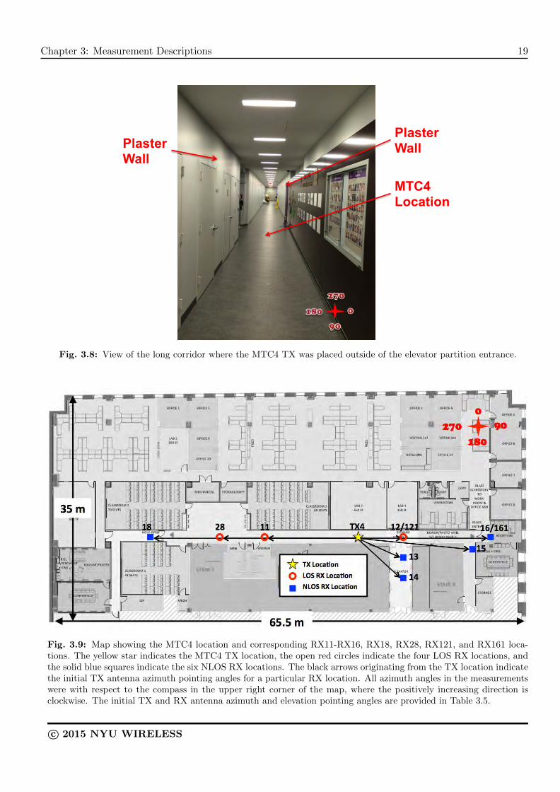
Chapter 3: Measurement Descriptions 19
MTC4 Location
Plaster Wall Plaster
Wall
Fig. 3.8: View of the long corridor where the MTC4 TX was placed outside of the elevator partition entrance.
Fig. 3.9: Map showing the MTC4 location and corresponding RX11-RX16, RX18, RX28, RX121, and RX161 loca-tions. The yellow star indicates the MTC4 TX location, the open red circles indicate the four LOS RX locations, andthe solid blue squares indicate the six NLOS RX locations. The black arrows originating from the TX location indicatethe initial TX antenna azimuth pointing angles for a particular RX location. All azimuth angles in the measurementswere with respect to the compass in the upper right corner of the map, where the positively increasing direction isclockwise. The initial TX and RX antenna azimuth and elevation pointing angles are provided in Table 3.5.
c© 2015 NYU WIRELESS

20 Chapter 3: Measurement Descriptions
Table 3.5: TX and RX location IDs, T-R separation distances, initial TX and RX antenna azimuth and elevationpointing angles for each TX-RX location combination, and environment types for the co- and cross-polarization antennaconfiguration measurements for the MTC4 TX location. All angle configurations are identical for the 28 GHz and 73GHz measurements.
TX RXT-R TX TX RX RX
EnvironmentDistance (m) Azimuth(◦) Elevation(◦) Azimuth(◦) Elevation(◦)
MTC4 11 12.7 270 -5 90 5 LOS
MTC4 12 7.1 90 -8 270 8 LOS
MTC4 121 7.1 90 -8 270 8 LOS
MTC4 13 8.2 120 -7 300 7 NLOS
MTC4 14 10.8 139 -5 319 5 NLOS
MTC4 15 20.8 100 -3 280 3 NLOS
MTC4 16 20.6 90 -3 270 3 NLOS
MTC4 161 20.6 90 -3 270 3 LOS
MTC4 18 33.0 270 -2 90 2 NLOS
MTC4 28 21.3 270 -3 90 3 LOS
3.1.5 MTC5 and corresponding RX locations
The fifth TX location (MTC5) was located in a classroom adjacent to the long corridor on the 9th floorof 2 MetroTech Center. Eight RX locations (RX8, RX19, and RX28-RX33) were selected, all in NLOSenvironments. Fig. 3.10 displays the classroom environment for the MTC5 TX location.
Fig. 3.11 displays the RX locations placed outside of the classroom on the 9th floor of 2 MetroTech Center.The blockage materials included numerous drywalls outside the classroom and along the corridor, and metaldoors at the rear entrance of NYU WIRELESS. Table 3.6 lists the T-R separation distances, initial TXand RX antenna azimuth and elevation pointing angle combinations, and environments for both the co- andcross-polarization measurements, for each TX-RX location combination.
MTC5 Location
Drywall
Classroom Entrance (Glass Door)
Fig. 3.10: View of the inside of the classroom where the MTC5 TX location was placed, surrounded by desks andchairs.
c© 2015 NYU WIRELESS

Chapter 3: Measurement Descriptions 21
Fig. 3.11: Map displaying the MTC5 TX location, and RX8, RX19, and RX28-RX33 locations. The yellow starindicates the MTC5 TX location and the solid blue squares indicate the eight NLOS RX locations. The black arrowsoriginating from the TX location indicate the initial TX antenna azimuth pointing angles for a particular RX location.All azimuth angles in the measurements were with respect to the compass in the upper right corner of this figure,where the positively increasing direction is clockwise. The initial TX and RX antenna azimuth and elevation pointingangles are provided in Table 3.6.
Table 3.6: TX and RX location IDs, T-R separation distances, initial TX and RX antenna azimuth and elevationpointing angles for the each TX-RX location combination, and environment types for the co- and cross-polarizationantenna configuration measurements for the MTC5 TX location. All angle configurations are identical for the 28 GHzand 73 GHz measurements.
TX RXT-R TX TX RX RX
EnvironmentDistance (m) Azimuth(◦) Elevation(◦) Azimuth(◦) Elevation(◦)
MTC5 8 3.9 9 -14 189 14 NLOS
MTC5 19 6.9 180 -8 0 8 NLOS
MTC5 28 15.6 106 -4 286 4 NLOS
MTC5 29 15.0 90 -4 270 4 NLOS
MTC5 30 11.4 127 -5 307 5 NLOS
MTC5 31 13.9 139 -4 319 4 NLOS
MTC5 32 31.2 90 -2 270 2 NLOS
MTC5 33 9.1 193 -6 13 6 NLOS
c© 2015 NYU WIRELESS

22 Chapter 3: Measurement Descriptions
3.2 System Descriptions
Two 400 Mcps broadband sliding correlator channel sounders were employed, one at 28 GHz and the otherat 73 GHz, both consisting of similar architectures with varying Intermediate Frequency (IF) and LocalOscillator (LO) frequencies, as well as interchangeable RF up- and down-converter front-ends.
3.2.1 Transmitter Hardware
The TX sides of the channel sounding systems used for the 28 GHz and 73 GHz measurements are displayedin Figs 3.12 and 3.13, respectively. The systems used state-of-the-art signal generators provided by NationalInstruments (NI) and PhaseMatrix for an Intermediate Frequency (IF) of 5.4 GHz and 5.625 GHz and aLocal Oscillator (LO) frequency of 22.6 GHz and 22.625 GHz (subsequently tripled to 67.875 GHz) forthe 28 GHz and 73 GHz measurements, respectively. At the TX, we generated a maximal length 2047pseudorandom noise (PN) sequence (or pseudorandom binary sequence (PRBS)) clocked at 400 MHz, whichwas mixed with the IF of 5.4 GHz or 5.625 GHz, and was then modulated with either the LO of 22.6 GHzor 67.875 GHz, allowing us to reach either center frequency of 28 GHz or 73.5 GHz, respectively, resultingin an RF signal with 800 MHz null-to-null bandwidth. The 22.625 GHz LO frequency used in the 73 GHzsystem was frequency-tripled inside the RF up-converter to achieve an LO of 67.875 GHz. The RF signal wastransmitted through a highly-directional horn antenna (mounted to a waveguide output) with 15 dBi of gain(28.8◦ azimuth HPBW) and 20 dBi of gain (15◦ azimuth HPBW) for the 28 GHz and 73 GHz measurements,respectively.
Fig. 3.12: Block diagram of the 28 GHz transmitter. The TX PN generator produced a 400 Mcps PN sequence thatwas modulated by a 5.4 GHz IF and then multiplied by a 22.6 GHz LO, thus upconverted to a 28 GHz centered RFsignal. The RF signal was then transmitted through a highly-directional horn antenna with 15 dBi of gain and 28.8◦
azimuth HPBW.
3.2.2 Receiver Hardware
Figs. 3.14 and 3.15 display the block diagrams of the 28 GHz and 73 GHz RX systems, respectively. Inthe down-converter stage, the received 28 GHz or 73.5 GHz centered spread spectrum RF signal was down-converted into the 5.4 GHz or 5.625 GHz IF, and was then further demodulated using an IF-stage LOof 5.4 GHz or 5.625 GHz, into the in-phase I and quadrature Q, baseband signals. Both the I and Qbaseband components were then mixed with a PRBS sequence identical to the transmitted signal, but at aslightly slower rate of 399.95 Mcps, which produced an impulse when both codes were aligned in time. Thecross-correlation mixing operation reduced the bandwidth of the I and Q signals to 50 kHz due to the time
c© 2015 NYU WIRELESS
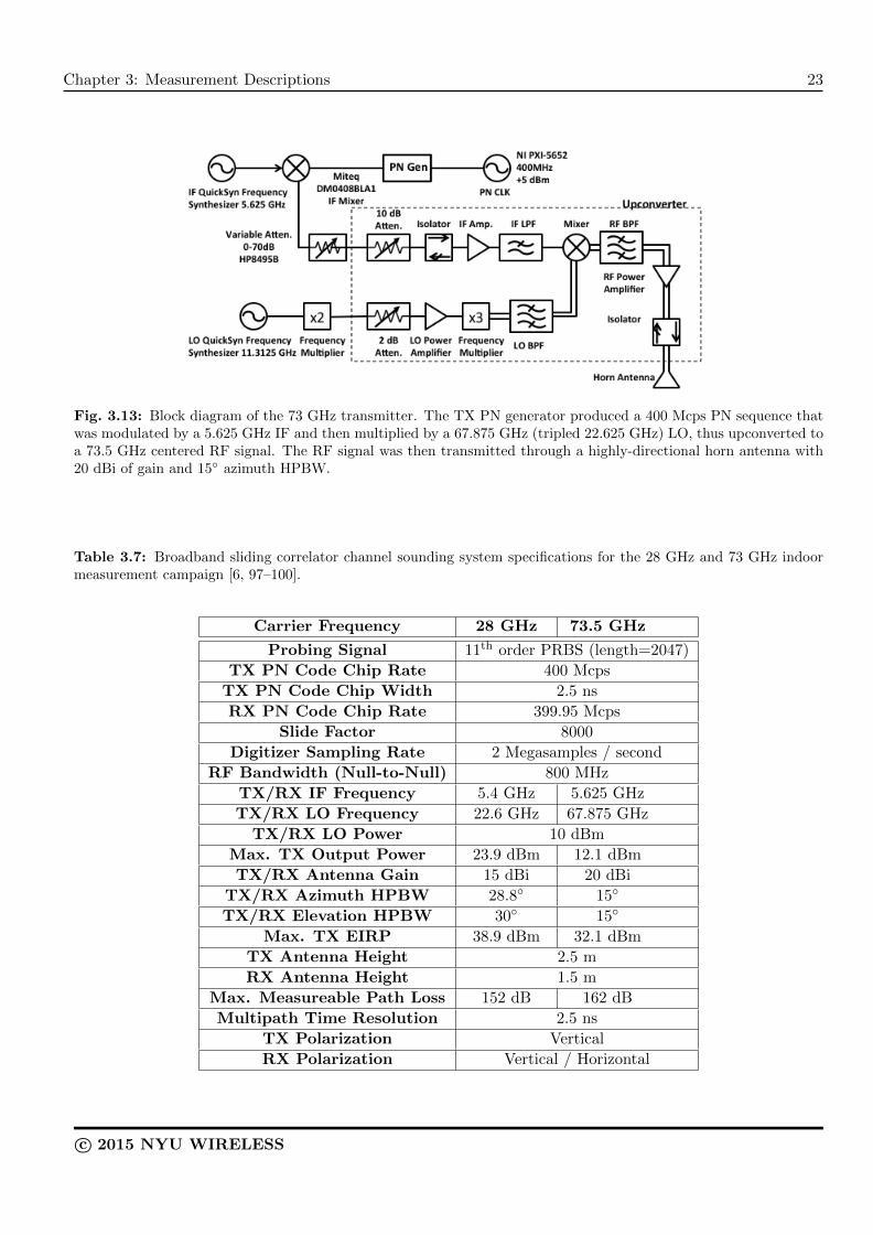
Chapter 3: Measurement Descriptions 23
Fig. 3.13: Block diagram of the 73 GHz transmitter. The TX PN generator produced a 400 Mcps PN sequence thatwas modulated by a 5.625 GHz IF and then multiplied by a 67.875 GHz (tripled 22.625 GHz) LO, thus upconverted toa 73.5 GHz centered RF signal. The RF signal was then transmitted through a highly-directional horn antenna with20 dBi of gain and 15◦ azimuth HPBW.
Table 3.7: Broadband sliding correlator channel sounding system specifications for the 28 GHz and 73 GHz indoormeasurement campaign [6, 97–100].
Carrier Frequency 28 GHz 73.5 GHz
Probing Signal 11th order PRBS (length=2047)
TX PN Code Chip Rate 400 Mcps
TX PN Code Chip Width 2.5 ns
RX PN Code Chip Rate 399.95 Mcps
Slide Factor 8000
Digitizer Sampling Rate 2 Megasamples / second
RF Bandwidth (Null-to-Null) 800 MHz
TX/RX IF Frequency 5.4 GHz 5.625 GHz
TX/RX LO Frequency 22.6 GHz 67.875 GHz
TX/RX LO Power 10 dBm
Max. TX Output Power 23.9 dBm 12.1 dBm
TX/RX Antenna Gain 15 dBi 20 dBi
TX/RX Azimuth HPBW 28.8◦ 15◦
TX/RX Elevation HPBW 30◦ 15◦
Max. TX EIRP 38.9 dBm 32.1 dBm
TX Antenna Height 2.5 m
RX Antenna Height 1.5 m
Max. Measureable Path Loss 152 dB 162 dB
Multipath Time Resolution 2.5 ns
TX Polarization Vertical
RX Polarization Vertical / Horizontal
c© 2015 NYU WIRELESS

24 Chapter 3: Measurement Descriptions
dilation properties of sliding correlation (slide factor of 8000) [49, 101, 102]. The subsequent I and Q voltagesignals then passed through a 100 kHz low pass filter and were then individually sampled at 2 MS/s. UsingLabVIEW software, the digital I and Q samples (I2+Q2) were squared and then summed to generate the rawPDP of the channel. Each sampled signal resulted in a power delay profile (PDP) that was 60,000 sampleslong. In order to increase the SNR of the received signal, 20 successive PDPs were averaged to obtain arecorded PDP for each individual measurement†. At the receiver, directionality across a large portion of theazimuth and elevation planes was made possible by mechanically steering the directional receiver antennaswith gimbals controlled by LabVIEW software. The flexibility in maneuvering the RX antennas allowedmany different angles of arrival (AOAs) over the entire 360◦ azimuth plane to be measured in additionto many elevation planes. Future measurements will use recently upgraded synchronization between theTX and RX to recover true propagation delay of recorded PDPs. Table 3.7 provides the channel sounderspecifications for the 28 GHz and 73 GHz measurement systems.
Fig. 3.14: Block diagram of the RX system used to characterize the 28 GHz indoor channel. The received signal wasdownconverted from the 28 GHz centered RF signal via an LO of 22.6 GHz, which was then subsequently demodulateddown to its I and Q baseband components via an IF-stage 5.4 GHz LO. A PN sequence identical to that at the TXwas generated, but at a slightly slower rate of 399.95 Mcps, and was then mixed with the received signal’s basebandI and Q signals, that were used to recover a time-dilated impulse response of the channel.
3.3 Measurement Procedure
The indoor measurement days started and ended with a free space system calibration routine at a knowndistance of 4 m, with vertically-polarized TX and RX antennas at heights of 2 m. The purpose of calibrationwas to find the linear range and gain of the RX system in order to recover the true received power fromeach individually recorded field measurement. Calibration was necessary at the end of the measurement
†Results in this report may be slightly different than those initially reported in [103, 104] due to this updated averagingmethod and the use of a more stringent 5 dB SNR thresholding algorithm described in [105].
c© 2015 NYU WIRELESS
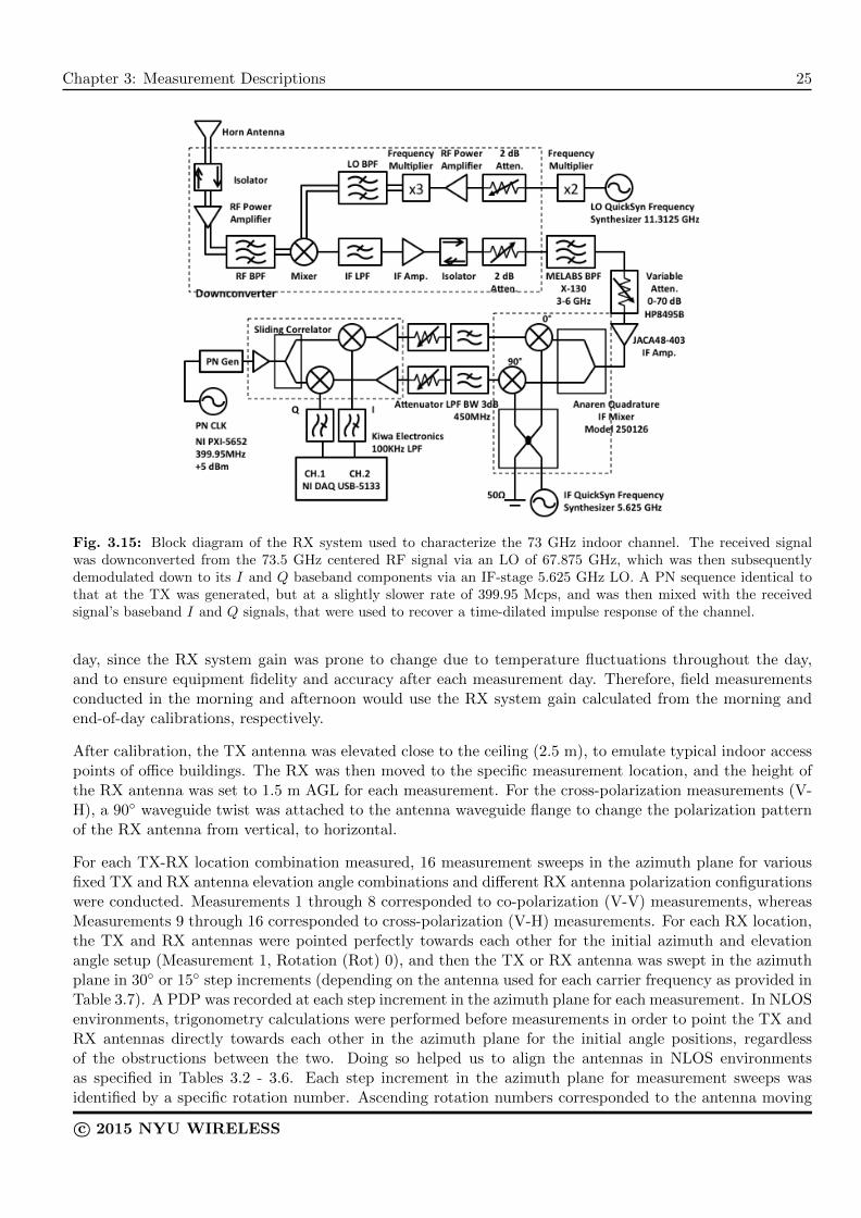
Chapter 3: Measurement Descriptions 25
Fig. 3.15: Block diagram of the RX system used to characterize the 73 GHz indoor channel. The received signalwas downconverted from the 73.5 GHz centered RF signal via an LO of 67.875 GHz, which was then subsequentlydemodulated down to its I and Q baseband components via an IF-stage 5.625 GHz LO. A PN sequence identical tothat at the TX was generated, but at a slightly slower rate of 399.95 Mcps, and was then mixed with the receivedsignal’s baseband I and Q signals, that were used to recover a time-dilated impulse response of the channel.
day, since the RX system gain was prone to change due to temperature fluctuations throughout the day,and to ensure equipment fidelity and accuracy after each measurement day. Therefore, field measurementsconducted in the morning and afternoon would use the RX system gain calculated from the morning andend-of-day calibrations, respectively.
After calibration, the TX antenna was elevated close to the ceiling (2.5 m), to emulate typical indoor accesspoints of office buildings. The RX was then moved to the specific measurement location, and the height ofthe RX antenna was set to 1.5 m AGL for each measurement. For the cross-polarization measurements (V-H), a 90◦ waveguide twist was attached to the antenna waveguide flange to change the polarization patternof the RX antenna from vertical, to horizontal.
For each TX-RX location combination measured, 16 measurement sweeps in the azimuth plane for variousfixed TX and RX antenna elevation angle combinations and different RX antenna polarization configurationswere conducted. Measurements 1 through 8 corresponded to co-polarization (V-V) measurements, whereasMeasurements 9 through 16 corresponded to cross-polarization (V-H) measurements. For each RX location,the TX and RX antennas were pointed perfectly towards each other for the initial azimuth and elevationangle setup (Measurement 1, Rotation (Rot) 0), and then the TX or RX antenna was swept in the azimuthplane in 30◦ or 15◦ step increments (depending on the antenna used for each carrier frequency as provided inTable 3.7). A PDP was recorded at each step increment in the azimuth plane for each measurement. In NLOSenvironments, trigonometry calculations were performed before measurements in order to point the TX andRX antennas directly towards each other in the azimuth plane for the initial angle positions, regardlessof the obstructions between the two. Doing so helped us to align the antennas in NLOS environmentsas specified in Tables 3.2 - 3.6. Each step increment in the azimuth plane for measurement sweeps wasidentified by a specific rotation number. Ascending rotation numbers corresponded to the antenna moving
c© 2015 NYU WIRELESS

26 Chapter 3: Measurement Descriptions
in the counterclockwise direction with respect to the compass in Fig. 3.1, while descending rotation numberscorresponded to the antenna moving in the clockwise direction. Tables 3.2 - 3.6 indicate the Measurement1, Rot 0 TX and RX antenna azimuth and elevation pointing angles for each specific TX-RX locationcombination measured for both the 28 GHz and 73 GHz measurements.
The list of items to follow indicates the change in TX and/or RX antenna azimuth and elevation anglesfor the Rot 0 pointing direction of Measurements 1 through 8 (V-V). Measurements 9 through 16 (V-H)are identical to 1 through 8, except the RX antenna was configured for horizontal polarization. For RXsweeps (Measurements 1-5, 7, 9-13, and 15), the TX antenna was fixed in the azimuth and elevation planeswith the RX antenna elevation fixed, and then swept in step increments in the azimuth plane. For TXsweeps (Measurements 6, 8, 14, and 16), the RX antenna was fixed in the azimuth and elevation planeswith the TX antenna elevation fixed, and then swept in step increments in the azimuth plane. RX antennasweeps are also known as AOA sweeps, and TX antenna sweeps are also known as AOD sweeps. For eachmeasurement sweep and at each incremental step, a PDP was recorded at the RX. The detailed descriptionof each measurement sweep is listed below. The measurement sweep descriptions hold true for both LOSand NLOS environments.
• Measurement 1 (M1): The TX and RX antennas were pointed directly towards each other on boresightin both the azimuth and elevation planes (for LOS or NLOS environments). The RX antenna was thenswept in the azimuth plane in steps of 30◦ or 15◦, for a fixed TX antenna at the boresight azimuthand elevation angles.
• Measurement 2 (M2): With respect to the boresight angle in elevation, the RX antenna was uptiltedby 30◦ or 15◦ and then swept in the azimuth plane in steps of 30◦ or 15◦, for a fixed TX antenna atthe boresight azimuth and elevation angles.
• Measurement 3 (M3): With respect to the boresight angle in elevation, the RX antenna was downtiltedby 30◦ or 15◦ and then swept in the azimuth plane in steps of 30◦ or 15◦, for a fixed TX antenna atthe boresight azimuth and elevation angles.
• Measurement 4 (M4): With respect to the boresight angle in elevation, the TX antenna was uptiltedby 30◦ or 15◦. The RX antenna was fixed at the boresight elevation angle, and then swept in theazimuth plane in steps of 30◦ or 15◦.
• Measurement 5 (M5): With respect to the boresight angle in elevation, the TX antenna was downtiltedby 30◦ or 15◦. The RX antenna was fixed at the boresight elevation angle, and then swept in theazimuth plane in steps of 30◦ or 15◦.
• Measurement 6 (M6): The TX and RX antennas were pointed directly towards each other on boresightin both the azimuth and elevation planes. The TX antenna was then swept in the azimuth plane insteps of 30◦ or 15◦, for a fixed RX antenna at the boresight azimuth and elevation angles.
• Measurement 7 (M7): This measurement was an RX sweep with the TX antenna set to the secondstrongest AOD in the azimuth and elevation plane. The second strongest AOD was determined bycomparing the trigger level from all the AODs during Measurement 6, except for the angles corre-sponding to the main angle of arrival. The RX antenna was fixed at the boresight elevation angle andthen swept in steps of 30◦ or 15◦ in the azimuth plane.
• Measurement 8 (M8): This measurement corresponds to the second TX sweep with TX antennaeither uptilted or downtilted by 30◦ or 15◦ after determining the elevation plane with the strongestreceived power from Measurement 4 and Measurement 5 during field measurements. The RX antennawas pointed towards the initial boresight azimuth and elevation angles, and the TX was uptilted ordowntilted by 30◦ or 15◦, and then swept in steps of 30◦ or 15◦ in the azimuth plane.
c© 2015 NYU WIRELESS
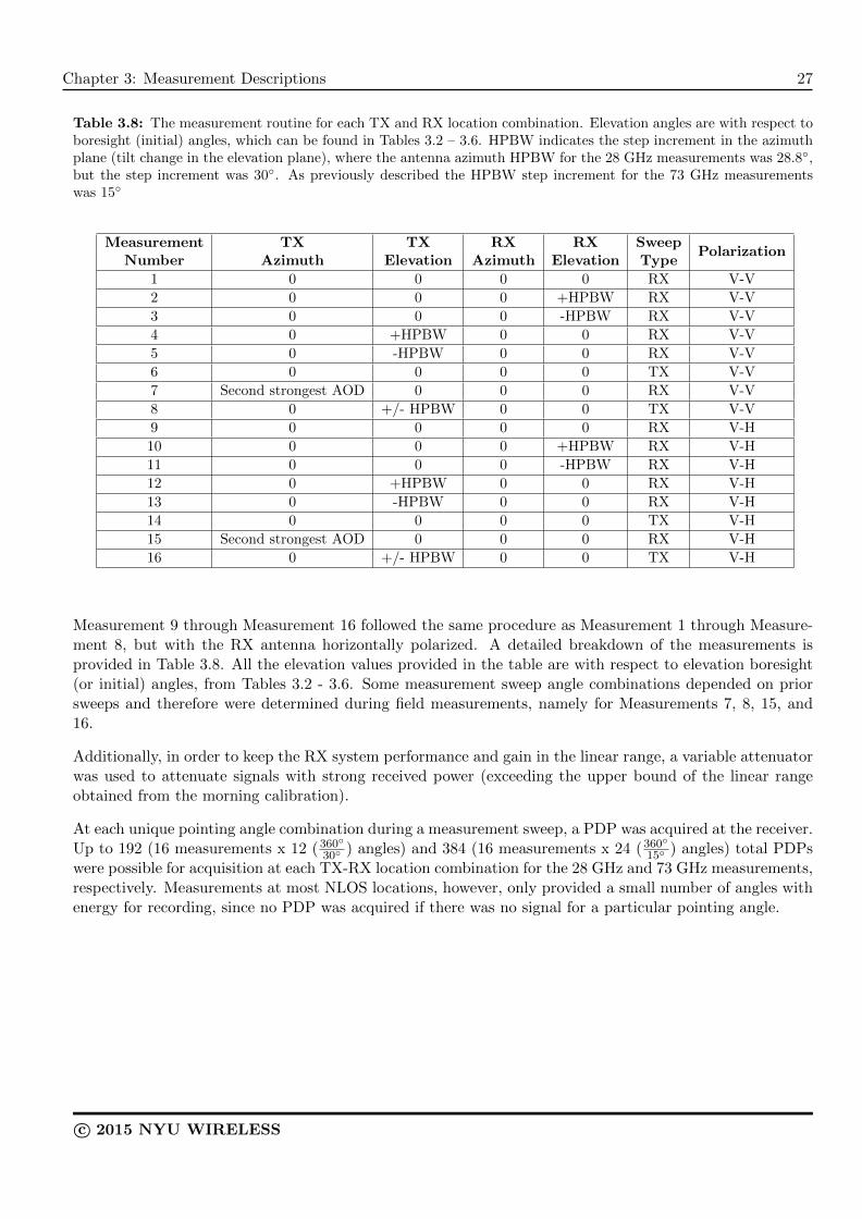
Chapter 3: Measurement Descriptions 27
Table 3.8: The measurement routine for each TX and RX location combination. Elevation angles are with respect toboresight (initial) angles, which can be found in Tables 3.2 – 3.6. HPBW indicates the step increment in the azimuthplane (tilt change in the elevation plane), where the antenna azimuth HPBW for the 28 GHz measurements was 28.8◦,but the step increment was 30◦. As previously described the HPBW step increment for the 73 GHz measurementswas 15◦
Measurement TX TX RX RX SweepPolarization
Number Azimuth Elevation Azimuth Elevation Type
1 0 0 0 0 RX V-V
2 0 0 0 +HPBW RX V-V
3 0 0 0 -HPBW RX V-V
4 0 +HPBW 0 0 RX V-V
5 0 -HPBW 0 0 RX V-V
6 0 0 0 0 TX V-V
7 Second strongest AOD 0 0 0 RX V-V
8 0 +/- HPBW 0 0 TX V-V
9 0 0 0 0 RX V-H
10 0 0 0 +HPBW RX V-H
11 0 0 0 -HPBW RX V-H
12 0 +HPBW 0 0 RX V-H
13 0 -HPBW 0 0 RX V-H
14 0 0 0 0 TX V-H
15 Second strongest AOD 0 0 0 RX V-H
16 0 +/- HPBW 0 0 TX V-H
Measurement 9 through Measurement 16 followed the same procedure as Measurement 1 through Measure-ment 8, but with the RX antenna horizontally polarized. A detailed breakdown of the measurements isprovided in Table 3.8. All the elevation values provided in the table are with respect to elevation boresight(or initial) angles, from Tables 3.2 - 3.6. Some measurement sweep angle combinations depended on priorsweeps and therefore were determined during field measurements, namely for Measurements 7, 8, 15, and16.
Additionally, in order to keep the RX system performance and gain in the linear range, a variable attenuatorwas used to attenuate signals with strong received power (exceeding the upper bound of the linear rangeobtained from the morning calibration).
At each unique pointing angle combination during a measurement sweep, a PDP was acquired at the receiver.Up to 192 (16 measurements x 12 (360
◦
30◦ ) angles) and 384 (16 measurements x 24 (360◦
15◦ ) angles) total PDPswere possible for acquisition at each TX-RX location combination for the 28 GHz and 73 GHz measurements,respectively. Measurements at most NLOS locations, however, only provided a small number of angles withenergy for recording, since no PDP was acquired if there was no signal for a particular pointing angle.
c© 2015 NYU WIRELESS

This page is intentionally left blank.
Chapter 4
Large-Scale Path Loss Models
Large-scale path loss models estimate the attenuation over distance of propagating signals, and are vital fordesigning communications systems. Different types (deterministic, empirical, and stochastic) of large-scalepath loss models exist, but measurement-based path loss models provide realistic insight into propagationcharacteristics of a wireless channel [105, 106].
4.1 Single Frequency Path Loss Models
A common path loss model is the close-in free space reference distance (CI) path loss model provided inEq. (4.1) and parameterized by the average path loss exponent (PLE) n:
PLCI(f, d)[dB] = FSPL(f, d0) + 10n log10
(d
d0
)+XCI
σ for d ≥ d0, where d0 = 1 m (4.1)
where XCIσ is a zero mean Gaussian random variable with standard deviation σ in dB (large-scale channel
fluctuations due to shadowing [49]). The CI model uses a physically-based reference distance d0, where
FSPL(f, d0) = 10 log10
(4πd0λ
)2. The CI path loss model is found by determining the PLE n via the minimum
mean-square error (MMSE) approach that fits the measured data with smallest error (by minimizing σ) usinga true physical anchor point that expresses the free space transmitted power from the TX antenna out to theclose-in distance d0. The closed-form expression for optimizing the CI PLE can be found in Appendix A. Forthe mmWave CI model, d0 = 1 m is used, proposed as a standard in [25, 105]. High gain directional antennasmay have far-field radiation patterns (Fraunhofer distances) greater than 1 m from the antenna, but the CIpath loss model can easily be reverted back to a 1 m reference distance by assuming that the far-field beginsat 1 m (even if it does not). The error between the near- and far-field will not be significant in communicationanalysis using a 1 m reference distance, since very few users would ever be this close to the TX antenna,and close-in users will have extremely strong signals and little path loss [105]. Standardizing to a d0 = 1 mreference distance allows for easy model comparison between different frequency bands and measurementsfrom other researchers, and allows closed-form computation in analysis, and intuitive computation of pathloss or received power without a calculator, since the power decays by 10n dB per decade of distance beyond1 m [105]. The CI path loss model may be used for estimating path loss from either cross- or co-polarizationmeasurements, or for a generalized data set that combines both co- and cross-polarized (combined polarized)measurements (as would occur in a practical cellular system with random device orientations). As shownin [105], the single parameter CI model may be used for multiple frequencies with good accuracy in outdoorchannels, but as shown subsequently, a two parameter variation of the CI model offers a better fit for indoorchannels.
30 Chapter 4: Large-Scale Path Loss Models
An extension of the basic (CI) path loss model for the special case of cross-polarization propagation is toadd a constant attenuation factor known as the cross-polarization discrimination (XPD) factor, that bestfits the measured data via an MMSE method [22, 24, 49, 107] given by:
PLCIX(f, d)[dB] = FSPL(f, d0) + 10n(V-V) log10
(d
d0
)+ XPD[dB] +XCIX
σ (4.2)
This model, which we call the close-in reference distance with XPD (CIX) path loss model, is similar tothe constant floor attenuation model introduced in [42, 43, 96], and uses the co-polarization PLE in (4.1) todetermine the best fit XPD factor caused by antenna polarization mismatch. Instead of solving for a PLEfor cross-polarized measured path loss in (4.1), the CIX model uses the PLE found from co-polarized an-tenna measurements at identical locations of cross-polarized measurements, and adds an optimized constantattenuation (XPD). One simply solves for the optimal XPD value (in dB) via the MMSE method that fitsthe measured cross-polarized path loss data with the smallest error (by minimizing σ). As seen from (4.2),the CIX model uses the optimum attenuation factor (XPD) in dB that is added to the CI model to minimizethe error between the estimator and measured cross-polarized path loss. In (4.2), n(V-V) represents theco-polarization PLE determined from measurements, as provided in Table 5.2, XPD is the optimized cross-polarization attenuation factor in dB, and XCIX
σ is the zero mean Gaussian (in dB) shadow fading randomvariable for the CIX model in (4.2) that describes the large-scale variation of signal power about mean pathloss and constant XPD attenuation term as a function of distance. The CIX model provides the best-fit tothe cross-polarized data (minimizes error via MMSE), while using the co-polarized PLE from (4.1) and a 1m free space reference distance. The CIX model closed-form expressions for optimizing the XPD value aregiven in Appendix A.
The floating-intercept (FI) path loss model is used in the WINNER II and 3GPP standards [108, 109]. Thismodel requires two parameters and does not consider a physically-based anchor to the transmitted power,and has a similar form to (4.1):
PLFI(d)[dB] = α+ 10 · β log10(d) +XFIσ (4.3)
where α is the floating-intercept in dB (different than a FSPL reference), and β is the slope of the line(different than a PLE), also with a zero mean Gaussian (in dB) shadow fading random variable XFI
σ whichdescribes large-scale signal fluctuations about the mean path loss over distance. Similar to the CI and CIXmodels, the best-fit involves solving for α and β to minimize σ and the closed-form optimized solutions areprovided in Appendix A. Note that (4.3) requires two model parameters, whereas the CI model only requireda single parameter, the PLE. Previous work indicated that the CI and FI path loss models produce verysimilar shadow fading standard deviations in outdoor mmWave channels [105, 110–112], casting doubt onthe value of using an extra modeling parameter when there is a lack of physical relationship to transmittedpower.
4.2 Multi-Frequency Path Loss Models
Standards bodies and modeling groups are also interested in multi-frequency path loss models in order tohave a general form/model to cover a broad range of frequencies and measurements. The CI model (4.1)can be used for both single and multi-frequency datasets. A multi-frequency three parameter model knownas the alpha-beta-gamma (ABG) model includes a frequency dependent and distance-dependent term todescribe path loss at various frequencies [112, 113]. The ABG model equation is given by (4.4):
PLABG(f, d)[dB] = 10α log10
(d
d0
)+ β + 10γ log10
(f
f0
)+XABG
σ , where d0 = 1 m, f0 = 1 GHz (4.4)
c© 2015 NYU WIRELESS

Chapter 4: Large-Scale Path Loss Models 31
where α and γ are coefficients that describe the distance and frequency dependence on path loss, β is anoptimized offset in path loss, f is the frequency in GHz and XABG
σ is Gaussian random variable representingthe shadowing or large-scale signal fluctuations about the mean path loss over distance. The ABG model isan extension of the FI model for multiple frequencies, and reverts to the FI model (when setting γ = 0 or2) if only a single frequency is used. The ABG model is solved via MMSE to minimize σ by simultaneouslysolving for α, β, and γ. Note that the ABG model is identical to the CI model if we equate α in the ABGmodel in (4.4) with the PLE n in the CI model in (4.1), γ in (4.4) with the free space PLE of 2, and βin (4.4) with 20 log10(4π/c). Furthermore, the ABG model requires three parameters and the CI modelonly one parameter, and as shown subsequently, the additional two variables in the ABG model offer verylittle improvement in accuracy and have no tie to propagation physics [105]. The closed-form expressionsfor optimizing the ABG model parameters are described in Appendix A.
Similar to the CIX model, one may consider the alpha-beta-gamma with XPD factor (ABGX) model thatis used for the specific case of cross-polarized propagation measurements. The ABGX model is providedin (4.5):
PLABGX(f, d)[dB] = 10α log10
(d
d0
)+ β + 10γ log10
(f
f0
)+ XPD[dB] +XABGX
σ , where d0 = 1 m, f0 = 1 GHz
(4.5)
where the optimum α, β, and γ values found for the ABG co-polarized measurement locations are used tosolve for the XPD value using identical cross-polarized locations that minimizes σ via MMSE. The closed-form expressions that optimize the XPD factor for the ABGX model when using the optimized co-polarizedABG model parameters are provided in Appendix A.
A new simple two parameter multi-frequency model can be considered to be an extension of the CI model.The close-in free space reference distance with frequency weighting (CIF) path loss model is a multi-frequency,frequency weighted model that employs the same FSPL anchor at 1 m as the CI model. The CIF modelequation is presented in (4.6):
PLCIF(f, d)[dB] = FSPL(f, d0) + 10n
(1 + b
(f − f0f0
))log10
(d
d0
)+XCIF
σ , where d0 = 1 m (4.6)
where n denotes the distance dependency of path loss (e.g. the path loss exponent, or PLE), b is an intuitivemodel-fitting parameter that captures the amount of linear frequency dependency of path loss, thus modelingthe results here which show that path loss increases with frequency at a specific distance for indoor channels∗,f0 is a fixed reference frequency that serves as the balancing point for the linear frequency dependency ofthe PLE, and is based on the average of all frequencies represented by the model, and XCIF
σ is the zero meanGaussian random variable (in dB) that describes large-scale signal fluctuations about the mean path lossover distance.
In the multi-frequency CIF model, the parameter f0 is computed as the weighted frequency average of allmeasurement locations for each specific environment and antenna scenario, found by summing up the numberof measurement locations at a particular frequency and antenna scenario, multiplying by the correspondingfrequency, and dividing that number by the entire number of measurement locations taken over all frequenciesfor that specific environment and antenna scenario. Note that we round the calculated f0 to the nearestinteger in GHz. For example, the combined polarization omnidirectional multi-frequency models in thisreport used f0 = 51 GHz in LOS and f0 = 49 GHz in NLOS, based on the number of measured locationsat each frequency in each environment. With a specified f0, the MMSE method is used to simultaneously
∗As shown in [105], outdoor channels exhibit a PLE that does not have a strong frequency dependence – most of the frequencydependence is captured in the first meter of free space propagation. However, indoor channels, as shown here, have a PLE thatis much more frequency dependent and are more lossy as frequency increases.
c© 2015 NYU WIRELESS

32 Chapter 4: Large-Scale Path Loss Models
solve for the two model parameters b and n that minimize σ. The CIF model has a similar form as theABG model (both have a frequency term, distance term, and constant intercept term) but only requires twomodel parameters instead of three, while also including the close-in free space leverage point for maintaininga physical tie to the transmitter [105, 114]. The CIF closed-form expressions for the best fit model parametersare given in Appendix A.
A CIF XPD factor (CIFX) model naturally follows, similar to the CIX and ABGX models for estimatingpath loss with cross-polarized antennas over multiple frequencies. The CIFX model equation is providedin (4.7):
PLCIFX(f, d)[dB] = FSPL(f, d0) + 10n
(1 + b
(f − f0f0
))log10
(d
d0
)+ XPD[dB] +XCIFX
σ , where d0 = 1 m
(4.7)
where the n and b values found for the co-polarized CIF model and the same f0 parameter are used tosolve for the XPD that minimizes σ via MMSE. The closed-form expressions for optimizing the CIFX modelparameters are similar to the CIX and ABGX models and are provided in Appendix A. It is important tonote that the single frequency CI model (4.1) can also be used as a multi-frequency path loss model, whilerequiring only a single parameter, PLE [105].
The large-scale path loss models and parameters presented in the following chapter will be useful for deter-mining capacity and for modeling communication system performance, in addition to determining deploy-ment approaches. Co-channel interference is one of the most important factors to consider when designinga wireless system and network, and the large-scale models to follow in this report can be used to estimateand analyze interference from multiple sources [115, 116]. Estimating bit error rates (BER) for indoor officeenvironments is also vital in order to understand how actual deployments will perform [117]. Shadowingor the large-scale signal fluctuations around the mean path loss is also necessary to understand for radio-system design, and researchers were able to estimate and predict shadowing relatively well for an indooroffice environment at 900 MHz and 1900 MHz in the early 1990’s [118]. The same approach may also beapplicable for simulations at mmWave frequencies.
c© 2015 NYU WIRELESS

Chapter 5
Path Loss Model Parameters andAnalysis
Single frequency and multi-frequency path loss models and parameters are explained and studied in thefollowing chapter. The distances d in the models to follow are the 3D T-R separation distances from themeasurements. Additionally, both co- and cross-polarized path loss models and combined polarization pathloss models are given for directional and omnidirectional cases. For combining the polarization measure-ments, the co- and cross-polarized measurements were lumped into one dataset. For omnidirectional models,the measurements for co- and cross-polarized antennas for the same identical locations were considered sep-arate, since full antenna sweeps were conducted across large portions of the azimuth and elevation planes tosynthesize omnidirectional path loss at one location for a specific polarization configuration.
5.1 Directional Path Loss Models for Co- and Cross-Polarized Antennas
Directional path loss models are useful for modeling systems at mmWaves that may use directional antennasfor arbitrary direction pointing, beam steering, or beam combining techniques [119, 120]. Previous work at28, 38, 60, and 73 GHz in outdoor environments provided insights into directional path loss models [6, 99,105, 121–123]. Now, path loss models are given for 28 GHz and 73 GHz indoor channels.
The definitions for descriptors of the physical environments for directional path loss models are identical tothose used in [105], and are given in Table 5.1. Figs. 5.1a and 5.1b display the directional path loss scatterplots and best fit CI models (4.1) at 28 GHz in LOS and NLOS environments for co-polarization (V-V)and cross-polarization (V-H) antenna configurations, respectively. Each plot also shows the NLOS-best CIpath loss model (see Table 5.1) that considers only the strongest received power for each measured NLOSTX-RX location combination. For V-V antenna polarizations, the LOS PLE is 1.7 at 28 GHz and 1.6 at
Table 5.1: Path loss environment definitions for directional path loss models.
Setting Description
LOS Path loss determined for environments when TX and RX antennas are pointed at each other, aligned onboresight with no obstructions between them.
NLOS Path loss determined for environments when TX and RX antennas are separated by obstructions and thereis no clear optical path between the antennas. This scenario also includes the case where the TX and RXantennas have a clear line-of-sight path to one another, but the antennas are not aligned on boresight.
NLOS-best Path loss determined for the unique antenna pointing angles (in the azimuth and elevation planes) resultingin the strongest received power for each specific TX-RX location combination. This results from the singlestrongest measured PDP from the NLOS data at each TX-RX location combination.
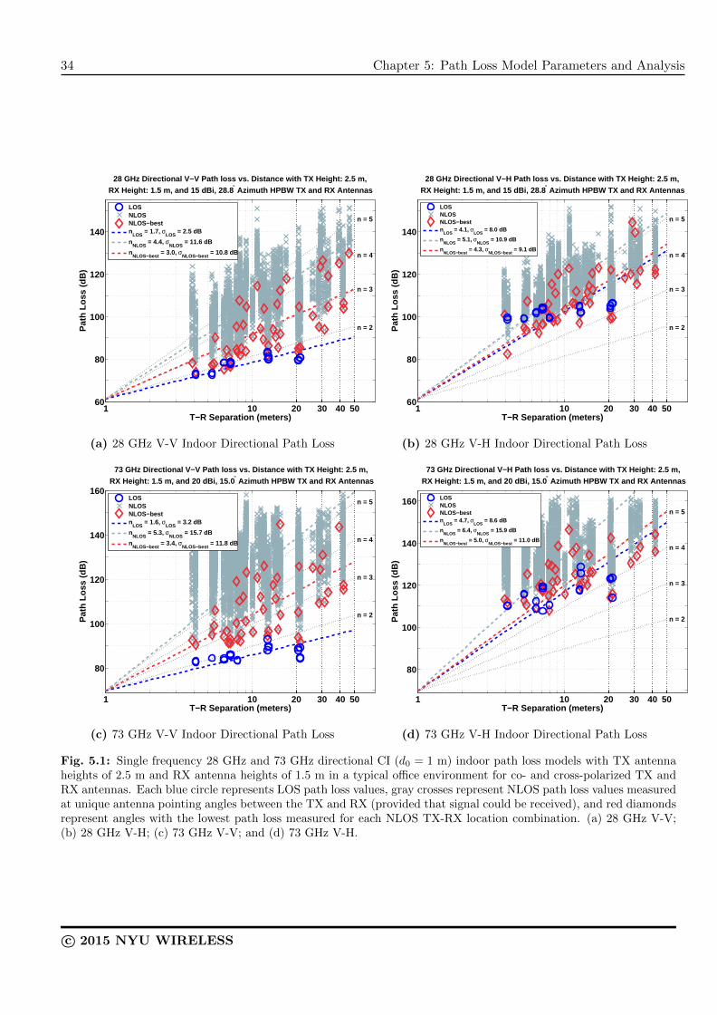
34 Chapter 5: Path Loss Model Parameters and Analysis
1 10 20 30 40 5060
80
100
120
140
n = 2
n = 3
n = 4
n = 5
T−R Separation (meters)
Pat
h Lo
ss (
dB)
28 GHz Directional V−V Path loss vs. Distance with TX Height: 2.5 m, RX Height: 1.5 m, and 15 dBi, 28.8 ° Azimuth HPBW TX and RX Antennas
LOSNLOSNLOS−bestn
LOS = 1.7, σ
LOS = 2.5 dB
nNLOS
= 4.4, σNLOS
= 11.6 dB
nNLOS−best
= 3.0, σNLOS−best
= 10.8 dB
(a) 28 GHz V-V Indoor Directional Path Loss
1 10 20 30 40 5060
80
100
120
140
n = 2
n = 3
n = 4
n = 5
T−R Separation (meters)
Pat
h Lo
ss (
dB)
28 GHz Directional V−H Path loss vs. Distance with TX Height: 2.5 m, RX Height: 1.5 m, and 15 dBi, 28.8 ° Azimuth HPBW TX and RX Antennas
LOSNLOSNLOS−bestn
LOS = 4.1, σ
LOS = 8.0 dB
nNLOS
= 5.1, σNLOS
= 10.9 dB
nNLOS−best
= 4.3, σNLOS−best
= 9.1 dB
(b) 28 GHz V-H Indoor Directional Path Loss
1 10 20 30 40 50
80
100
120
140
160
n = 2
n = 3
n = 4
n = 5
T−R Separation (meters)
Pat
h Lo
ss (
dB)
73 GHz Directional V−V Path loss vs. Distance with TX Height: 2.5 m, RX Height: 1.5 m, and 20 dBi, 15.0 ° Azimuth HPBW TX and RX Antennas
LOSNLOSNLOS−bestn
LOS = 1.6, σ
LOS = 3.2 dB
nNLOS
= 5.3, σNLOS
= 15.7 dB
nNLOS−best
= 3.4, σNLOS−best
= 11.8 dB
(c) 73 GHz V-V Indoor Directional Path Loss
1 10 20 30 40 50
80
100
120
140
160
n = 2
n = 3
n = 4
n = 5
T−R Separation (meters)
Pat
h Lo
ss (
dB)
73 GHz Directional V−H Path loss vs. Distance with TX Height: 2.5 m, RX Height: 1.5 m, and 20 dBi, 15.0 ° Azimuth HPBW TX and RX Antennas
LOSNLOSNLOS−bestn
LOS = 4.7, σ
LOS = 8.6 dB
nNLOS
= 6.4, σNLOS
= 15.9 dB
nNLOS−best
= 5.0, σNLOS−best
= 11.0 dB
(d) 73 GHz V-H Indoor Directional Path Loss
Fig. 5.1: Single frequency 28 GHz and 73 GHz directional CI (d0 = 1 m) indoor path loss models with TX antennaheights of 2.5 m and RX antenna heights of 1.5 m in a typical office environment for co- and cross-polarized TX andRX antennas. Each blue circle represents LOS path loss values, gray crosses represent NLOS path loss values measuredat unique antenna pointing angles between the TX and RX (provided that signal could be received), and red diamondsrepresent angles with the lowest path loss measured for each NLOS TX-RX location combination. (a) 28 GHz V-V;(b) 28 GHz V-H; (c) 73 GHz V-V; and (d) 73 GHz V-H.
c© 2015 NYU WIRELESS
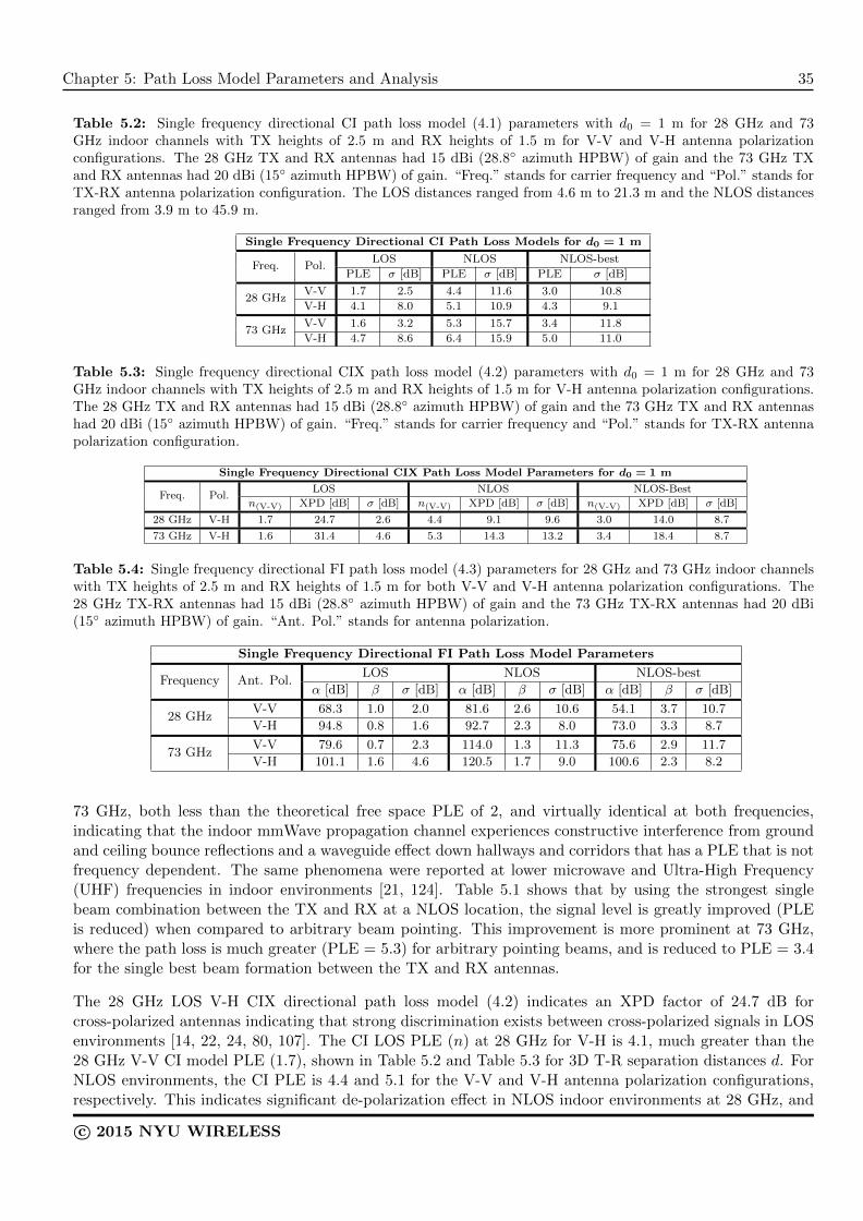
Chapter 5: Path Loss Model Parameters and Analysis 35
Table 5.2: Single frequency directional CI path loss model (4.1) parameters with d0 = 1 m for 28 GHz and 73GHz indoor channels with TX heights of 2.5 m and RX heights of 1.5 m for V-V and V-H antenna polarizationconfigurations. The 28 GHz TX and RX antennas had 15 dBi (28.8◦ azimuth HPBW) of gain and the 73 GHz TXand RX antennas had 20 dBi (15◦ azimuth HPBW) of gain. “Freq.” stands for carrier frequency and “Pol.” stands forTX-RX antenna polarization configuration. The LOS distances ranged from 4.6 m to 21.3 m and the NLOS distancesranged from 3.9 m to 45.9 m.
Single Frequency Directional CI Path Loss Models for d0 = 1 m
Freq. Pol.LOS NLOS NLOS-best
PLE σ [dB] PLE σ [dB] PLE σ [dB]
28 GHzV-V 1.7 2.5 4.4 11.6 3.0 10.8
V-H 4.1 8.0 5.1 10.9 4.3 9.1
73 GHzV-V 1.6 3.2 5.3 15.7 3.4 11.8
V-H 4.7 8.6 6.4 15.9 5.0 11.0
Table 5.3: Single frequency directional CIX path loss model (4.2) parameters with d0 = 1 m for 28 GHz and 73GHz indoor channels with TX heights of 2.5 m and RX heights of 1.5 m for V-H antenna polarization configurations.The 28 GHz TX and RX antennas had 15 dBi (28.8◦ azimuth HPBW) of gain and the 73 GHz TX and RX antennashad 20 dBi (15◦ azimuth HPBW) of gain. “Freq.” stands for carrier frequency and “Pol.” stands for TX-RX antennapolarization configuration.
Single Frequency Directional CIX Path Loss Model Parameters for d0 = 1 m
Freq. Pol.LOS NLOS NLOS-Best
n(V-V) XPD [dB] σ [dB] n(V-V) XPD [dB] σ [dB] n(V-V) XPD [dB] σ [dB]
28 GHz V-H 1.7 24.7 2.6 4.4 9.1 9.6 3.0 14.0 8.7
73 GHz V-H 1.6 31.4 4.6 5.3 14.3 13.2 3.4 18.4 8.7
Table 5.4: Single frequency directional FI path loss model (4.3) parameters for 28 GHz and 73 GHz indoor channelswith TX heights of 2.5 m and RX heights of 1.5 m for both V-V and V-H antenna polarization configurations. The28 GHz TX-RX antennas had 15 dBi (28.8◦ azimuth HPBW) of gain and the 73 GHz TX-RX antennas had 20 dBi(15◦ azimuth HPBW) of gain. “Ant. Pol.” stands for antenna polarization.
Single Frequency Directional FI Path Loss Model Parameters
Frequency Ant. Pol.LOS NLOS NLOS-best
α [dB] β σ [dB] α [dB] β σ [dB] α [dB] β σ [dB]
28 GHzV-V 68.3 1.0 2.0 81.6 2.6 10.6 54.1 3.7 10.7
V-H 94.8 0.8 1.6 92.7 2.3 8.0 73.0 3.3 8.7
73 GHzV-V 79.6 0.7 2.3 114.0 1.3 11.3 75.6 2.9 11.7
V-H 101.1 1.6 4.6 120.5 1.7 9.0 100.6 2.3 8.2
73 GHz, both less than the theoretical free space PLE of 2, and virtually identical at both frequencies,indicating that the indoor mmWave propagation channel experiences constructive interference from groundand ceiling bounce reflections and a waveguide effect down hallways and corridors that has a PLE that is notfrequency dependent. The same phenomena were reported at lower microwave and Ultra-High Frequency(UHF) frequencies in indoor environments [21, 124]. Table 5.1 shows that by using the strongest singlebeam combination between the TX and RX at a NLOS location, the signal level is greatly improved (PLEis reduced) when compared to arbitrary beam pointing. This improvement is more prominent at 73 GHz,where the path loss is much greater (PLE = 5.3) for arbitrary pointing beams, and is reduced to PLE = 3.4for the single best beam formation between the TX and RX antennas.
The 28 GHz LOS V-H CIX directional path loss model (4.2) indicates an XPD factor of 24.7 dB forcross-polarized antennas indicating that strong discrimination exists between cross-polarized signals in LOSenvironments [14, 22, 24, 80, 107]. The CI LOS PLE (n) at 28 GHz for V-H is 4.1, much greater than the28 GHz V-V CI model PLE (1.7), shown in Table 5.2 and Table 5.3 for 3D T-R separation distances d. ForNLOS environments, the CI PLE is 4.4 and 5.1 for the V-V and V-H antenna polarization configurations,respectively. This indicates significant de-polarization effect in NLOS indoor environments at 28 GHz, and
c© 2015 NYU WIRELESS

36 Chapter 5: Path Loss Model Parameters and Analysis
Table 5.5: 28 GHz and 73 GHz multi-frequency directional path loss model parameters for the CI, CIX, CIF, CIFX,ABG, and ABGX models for LOS, NLOS, and NLOS-Best environments and scenarios. The CIX, CIFX, and ABGXcross-polarized models use the corresponding parameters found for their respective co-polarized models to find theXPD factor in dB that minimizes σ. “Pol.” stands for polarization configuration (either V-V or V-H).
28 GHz and 73 GHz Multi-Frequency Directional LOS Path Loss Model Parameters
Pol. PLE XPD σ
CI V-V 1.7 - 2.9 dB
CIX V-H 1.7 28.1 dB 4.7 dB
Pol. n b f0 XPD σ
CIF V-V 1.7 -0.07 52 GHz - 2.9 dB
CIFX V-H 1.7 -0.07 52 GHz 28.1 dB 5.0 dB
Pol. α β γ XPD σ
ABG V-V 0.9 43.6 1.8 - 2.1 dB
ABGX V-H 0.9 43.6 1.8 27.4 dB 4.9 dB
28 GHz and 73 GHz Multi-Frequency Directional NLOS Path Loss Model Parameters
Pol. PLE XPD σ
CI V-V 4.9 - 14.6 dB
CIX V-H 4.9 11.3 dB 13.3 dB
Pol. n b f0 XPD σ
CIF V-V 4.8 0.19 50 GHz - 13.9 dB
CIFX V-H 4.8 0.19 50 GHz 11.6 dB 11.8 dB
Pol. α β γ XPD σ
ABG V-V 1.9 27.5 4.3 - 11.1 dB
ABGX V-H 1.9 27.5 4.3 8.9 dB 8.7 dB
28 GHz and 73 GHz Multi-Frequency Directional NLOS-Best Path Loss Model Parameters
Pol. PLE XPD σ
CI V-V 3.2 - 11.5 dB
CIX V-H 3.2 16.0 dB 9.6 dB
Pol. n b f0 XPD σ
CIF V-V 3.2 0.13 50 GHz - 11.3 dB
CIFX V-H 3.2 0.13 50 GHz 16.1 dB 9.0 dB
Pol. α β γ XPD σ
ABG V-V 3.3 11.1 3.2 - 11.2 dB
ABGX V-H 3.3 11.1 3.2 16.2 dB 8.8 dB
is further emphasized by the XPD factor of 9.1 dB determined from (4.2), which is substantially less thanthe 24.7 dB XPD factor found for 28 GHz LOS indoor mmWave channels. Similar results were noticed forthe 73 GHz indoor channel, where LOS environments indicate an XPD factor of 31.4 dB, but only 14.3 dBfor NLOS environments.
Tables 5.2 and 5.3 show the CI (4.1) and CIX (4.2) path loss model parameters, respectively, with d0 = 1m at 28 GHz and 73 GHz in the indoor environments. Results in Table 5.2 are slightly different than thoseinitially published in [103] due to more stringent noise thresholding described in [105]. The 28 GHz and73 GHz LOS PLEs for V-V are 1.7 and 1.6, respectively, due to constructive interference, and the shadowfading (SF) standard deviations for V-V and V-H measurements at the two bands are approximately 3 dBand 8 dB for the CI models, respectively. The 73 GHz NLOS CI model shows a much larger shadow fadingstandard deviation that is approximately 16 dB for V-V and V-H configurations, indicating much largerfluctuations in received signal strength around the mean received power over all T-R separation distances,regardless of whether the polarizations are matched. The NLOS CIX models at 28 GHz and 73 GHz arebetter estimates of cross-polarization path loss compared to the CI model as they have smaller SF values(1.3 dB and 2.7 dB less) than the CI V-H path loss models.
c© 2015 NYU WIRELESS

Chapter 5: Path Loss Model Parameters and Analysis 37
1 10 20 30 40 5060
80
100
120
140
n = 2
n = 3
n = 4
n = 5
T−R Separation (meters)
Pat
h Lo
ss (
dB)
28 GHz Combined Polarization Directional Path loss Models with TX Height: 2.5 m, RX Height: 1.5 m, and 15 dBi, 28.8 ° Azimuth HPBW TX and RX Antennas
LOSNLOSNLOS−bestn
LOS = 2.9, σ
LOS = 13.3 dB
nNLOS
= 4.8, σNLOS
= 11.9 dB
nNLOS−best
= 3.0, σNLOS−best
= 10.8 dB
(a) 28 GHz combined polarization indoor directional pathloss
1 10 20 30 40 50
80
100
120
140
160
n = 2
n = 3
n = 4
n = 5
T−R Separation (meters)
Pat
h Lo
ss (
dB)
73 GHz Combined Polarization Directional Path loss Models with TX Height: 2.5 m, RX Height: 1.5 m, and 20 dBi, 15.0 ° Azimuth HPBW TX and RX Antennas
LOSNLOSNLOS−bestn
LOS = 3.1, σ
LOS = 16.8 dB
nNLOS
= 5.7, σNLOS
= 16.7 dB
nNLOS−best
= 3.4, σNLOS−best
= 11.8 dB
(b) 73 GHz combined polarization indoor directional pathloss
Fig. 5.2: Single frequency combined polarization 28 GHz and 73 GHz directional CI (d0 = 1 m) indoor path lossmodels with TX antenna heights of 2.5 m and RX antenna heights of 1.5 m in a typical office environment for LOSand NLOS environments. Each blue circle represents LOS path loss values, gray crosses represent NLOS path lossvalues measured at unique antenna pointing angles between the TX and RX (provided that signal could be received),and red diamonds represent angles with the lowest path loss measured for each NLOS TX-RX location combination.(a) 28 GHz; (b) 73 GHz.
Table 5.4 shows the parameters for the FI model, where it can be seen that α values can vary widelycompared to free space path loss at 1 m in LOS for V-V at 28 GHz (68.3 dB) and 73 GHz (79.6 dB), andin some environments by more than 20 to 30 dB. This reveals that the FI model lacks a physical link to thetransmitted signal power, and does not physically model what actually happens in a practical LOS or NLOSsystem where there are no obstructions, e.g., free space conditions, in the first several meters of propagation.Furthermore, the slope β of the mean least-squares fit line in (4.3) are close to or less than free space (β =2) in NLOS environments for both 28 GHz and 73 GHz with co- and cross-polarized antennas, which doesnot properly predict the intuitive fact that NLOS cross-polarized signals undergo much heavier attenuationwith distance than free space signals. This underscores the lack of intuition provided by the FI model whentrying to reconcile the physical effects of polarization and environmental loss with distance. The lack ofmeasurements or data samples is often the cause of α and β values that make no physical sense [105, 112].Post-processing methods that employ different thresholding techniques can also significantly change theparameters in the very sensitive FI model [105]. The results in Tables 5.2–5.4 indicate that there is littlevalue in using a model with more than 1 parameter, since the difference in standard deviation between theCI and FI models is very small, in most cases less than 1 dB.
With regards to the CI path loss model, the 73 GHz band is more lossy than the 28 GHz band in indoorNLOS environments. The 73 GHz band is initially 8.4 dB more lossy in the first meter of propagation,but as seen in Table 5.2, at greater distances the PLE is 0.9 greater for the V-V case, indicating that 73GHz NLOS propagation experiences an additional 9 dB per decade of distance more path loss beyond thefirst meter of propagation compared to 28 GHz. The smaller 73 GHz wavelength results in more diffusescattering and greater shadowing in the physical surroundings that weakens signals when compared to 28GHz in the NLOS indoor office environment. The carpeted floors, cubicle sound proofing, and textured wallsurfaces all likely contribute to greater attenuation due to diffusion at 73 GHz.
c© 2015 NYU WIRELESS
38 Chapter 5: Path Loss Model Parameters and Analysis
The CI model of (4.1) provides the benefit of simple comparisons of measurements across many frequencybands using just one parameter, since frequency dependent effects of the model are primarily contained in the1 m FSPL where a substantial amount of loss occurs, while the PLE value represents the environmental effectsof propagation that are less sensitive to frequency than the loss in the first meter. For outdoor mmWavechannels, the PLE was found to be only slightly sensitive to frequency [105]. However, Tables 5.2, 5.3, and 5.4show that for indoor channels, the environment provides additional and substantial frequency-dependent lossbeyond the first meter of free space propagation. Variations of the CI model as described in [3, 105, 114]and presented here with the CIF model (4.6) allow the PLE to vary with frequency.
Table 5.5 provides the 28 GHz and 73 GHz directional multi-frequency CI, CIX, CIF, CIFX, ABG andABGX path loss models for the directional LOS, NLOS, and NLOS-Best environments and scenarios. Themulti-frequency XPD models are used for cross-polarized measurements, as they result in lower standarddeviation and better minimization of σ compared to a non-XPD model, as noticed in the differences in σ whencomparing the CI cross-polarized (V-H) model and CIX model for directional single frequency measurementsin Table 5.2. The standard deviations for the three multi-frequency models are within 1 dB or so of eachother in LOS and NLOS environments, as shown in Table 5.5. The CI and CIF models have identical slopeparameters (PLE and n, respectively) in LOS (1.7) and NLOS-Best (3.2) environments and differ by only0.1 in NLOS. In the NLOS-Best environment, the ABG model has a similar slope parameter to the CI andCIF models (α) where the CI (PLE) and CIF (n) parameters are 3.2 and ABG α is 3.3. The CIX, CIFX,and ABGX LOS XPD models show that there is large polarization isolation in LOS environments, where theXPD factors are greater than 27 dB for each. The ABG and ABGX models have lower standard deviationsin a majority of scenarios when compared to the CIF and CIFX model, but not by much, except for thearbitrary pointing NLOS situation, where the ABG and ABGX models have a 2.8 dB and 3.1 dB lowerstandard deviation compared to the CIF and CIFX models. Note, however, the standard deviations for allthree models are large, over 11 dB in NLOS cases, and well within measurement error of 1-2 dB in typicalmeasurement campaigns. The ABGX and ABG models do not have a free space path loss leverage point,thus these models are not tied to true transmitted power, and as shown in [114], are much less stable oraccurate compared to models that use a free-space reference distance when used outside the measurementrange for which the model parameters were optimized for. The standard deviations of multi-frequency pathloss models for similar environments in Table 5.5 show just how closely the different directional path lossmodels predict path loss, with little difference in standard deviations observed for most cases (a majoritydiffer by less than 1 dB). The small differences in standard deviation suggest that the simpler, physics-basedCI, CIX, and CIF models may be better suited for closed-form analysis as well as standards work whendeveloping future mmWave indoor networks. As shown subsequently, the omnidirectional path loss modelsreveal even smaller differences between the CIF and ABG models.
5.2 Omnidirectional Path Loss Models for Co- and Cross-polarized An-tennas
While the preceding directional path loss models are useful for wireless systems using directional anten-nas [120, 125, 126], standards bodies rely on omnidirectional path loss models to allow arbitrary antennapatterns to be used for simulations. In order to synthesize an omnidirectional path loss model from di-rectional measurements, the antenna radiation patterns used during measurements must be de-embeddedor removed from the results [127]. This can be achieved by summing received powers (in the linear scale)from unique, non-overlapping pointing angle directional measurements (from adjacent angular bins) andafter subtracting the antennas gains, as implemented in [128, 129]. Since the measurement sweeps includedantenna pointing directions separated by approximately one antenna HPBW in the azimuth and elevationplanes, the summed directions are virtually orthogonal to each other in space, thereby avoiding over-counting
c© 2015 NYU WIRELESS

Chapter 5: Path Loss Model Parameters and Analysis 39
Table 5.6: Path loss definitions for omnidirectional path loss models.
Setting Description
LOS Path loss when there is a clear optical path between the TX and RX.
NLOS Path loss when the TX and RX are separated by obstructions and there is no clearoptical path between the TX and RX.
of received power or multipath energy [105, 129]. The raw omnidirectional path loss data used to generatethe omnidirectional path loss models presented in this report are provided in tabular form in Appendix B.
The same method used in [128] was performed on the 28 GHz and 73 GHz indoor directional data, wherefor each TX-RX location pair, the omnidirectional path loss between the ith TX location and the jth RXlocation was recovered from individual and non-overlapping pointing angle received powers in the azimuthand elevation planes following [105, 128, 129]:
PLi,j [dB] = Pti,j [dBm] − 10 log10
[∑z
∑y
∑x
∑w
Pri,j(θrw , φrx , θty , φtz
)[mW]
](5.1)
where θt and φt are the TX antenna pointing angles in the azimuth and elevation planes, respectively,θr and φr are the RX antenna pointing angles in the azimuth and elevation planes, where Pti,j is theomnidirectional transmit power, and the Pri,j values are the individual directional received powers from theunique pointing angles, with the antenna gains removed. The individual directional received powers werefound from the PDPs recorded for each unique antenna pointing angle, where power is the area under eachPDP. To ensure consistency with the omnidirectional path loss models presented in [105, 128], the samedescriptors of physical environments for omnidirectional path loss models were used in this article and aredefined in Table 5.6.
Figs. 5.3a – 5.3d display the CI (d0 = 1 m) and FI omnidirectional scatter plots and path loss models at28 GHz and 73 GHz for LOS and NLOS indoor office environments with separate V-V and V-H antennapolarization configurations. Table 5.7 lists the omnidirectional CI and FI path loss model parameters.Table 5.8 gives the CIX model parameters for the V-H omnidirectional cross-polarization scenarios. Thetables show that in LOS environments, the V-V CI model omnidirectional PLE is 1.1 and 1.3 at 28 GHzand 73 GHz, respectively. Similar to the directional V-V CI models, the omnidirectional PLEs are less thantheoretical free space path loss (n = 2), and not surprisingly show significantly lower loss than the directionalLOS channels. In NLOS environments for V-V antennas, the omnidirectional PLE is 2.7 and 3.2 at 28 GHzand 73 GHz, respectively, showing higher path loss at 73 GHz than at 28 GHz, likely due to increaseddiffuse scattering with shorter wavelengths at higher frequencies [7]. The NLOS directional V-V PLEs are4.4 and 5.3 at 28 GHz and 73 GHz, respectively, compared to the omnidirectional values of 2.7 and 3.2 at28 GHz and 73 GHz, respectively, showing that omnidirectional antennas would capture more energy thandirectional antennas, but offer less link margin (less distance range due to smaller antenna gain) [105, 129].
For cross-polarized antennas, the 28 GHz LOS (V-H PLE = 2.5) and NLOS (V-H PLE = 3.6) CIX omni-directional models resulted in attenuation XPD factors of 14.0 dB and 10.4 dB, respectively. The LOS andNLOS V-H PLEs for 73 GHz were 3.5 (XPD = 22.8 dB) and 4.5 (XPD = 15.4 dB), respectively, also indicat-ing higher path loss at 73 GHz as well as greater polarization discrimination. Similar to the directional pathloss models, for omnidirectional LOS channels, a lumped cross-polarization attenuation factor used in (4.2)yields a simple CIX path loss model with lower standard deviation (better fit) about the distance-dependentmean path loss compared to a traditional CI model for cross-polarized path loss data.
c© 2015 NYU WIRELESS

40 Chapter 5: Path Loss Model Parameters and Analysis
1 10 20 30 40 5060
80
100
120
n = 1
n = 2
n = 3
T−R Separation (meters)
Pat
h Lo
ss (
dB)
28 GHz Indoor Omnidirectional V−V Path Loss vs. Distancewith TX Height: 2.5 m and RX Height: 1.5 m
LOSNLOSn
LOS = 1.1, σ
LOS = 1.8 dB
nNLOS
= 2.7, σNLOS
= 9.6 dB
LOS (α, β, σ), = (60.4 dB, 1.2, 1.8 dB)NLOS (α, β, σ), = (51.3 dB, 3.5, 9.3 dB)
(a) 28 GHz V-V Indoor Omnidirectional Path Loss
1 10 20 30 40 5060
80
100
120
140
n = 1
n = 2
n = 3
n = 4
T−R Separation (meters)
Pat
h Lo
ss (
dB)
28 GHz Indoor Omnidirectional V−H Path Loss vs. Distancewith TX Height: 2.5 m and RX Height: 1.5 m
VH LOSVH NLOSCI−VV
LOS: n = 1.1, σ = 1.8 dB
CI−VVNLOS
: n = 2.7, σ = 9.6 dB
CIXLOS
: n = 1.1, XPD = 14.0 dB, σ = 1.5 dB
CIXNLOS
: n = 2.7, XPD = 10.4 dB, σ = 9.7 dB
FI−VHLOS
: α = 72.9 dB, β = 1.4, σ = 1.4 dB
FI−VHNLOS
: α = 61.9 dB, β = 3.6, σ = 9.4 dB
XPDLOS
= 14.0 dB
XPDNLOS
= 10.4 dB
(b) 28 GHz V-H Indoor Omnidirectional Path Loss
1 10 20 30 40 50
80
100
120
140
n = 1
n = 2
n = 3
n = 4
T−R Separation (meters)
Pat
h Lo
ss (
dB)
73 GHz Indoor Omnidirectional V−V Path Loss vs. Distancewith TX Height: 2.5 m and RX Height: 1.5 m
LOSNLOSn
LOS = 1.3, σ
LOS = 2.4 dB
nNLOS
= 3.2, σNLOS
= 11.3 dB
LOS (α, β, σ), = (77.9 dB, 0.5, 1.4 dB)NLOS (α, β, σ), = (76.3 dB, 2.7, 11.2 dB)
(c) 73 GHz V-V Indoor Omnidirectional Path Loss
1 10 20 30 40 50
80
100
120
140
160
n = 1
n = 2
n = 3
n = 4
T−R Separation (meters)
Pat
h Lo
ss (
dB)
73 GHz Indoor Omnidirectional V−H Path Loss vs. Distancewith TX Height: 2.5 m and RX Height: 1.5 m
VH LOSVH NLOSCI−VV
LOS: n = 1.3, σ = 2.4 dB
CI−VVNLOS
: n = 3.2, σ = 11.3 dB
CIXLOS
: n = 1.3, XPD = 22.8 dB, σ = 2.4 dB
CIXNLOS
: n = 3.2, XPD = 15.4 dB, σ = 8.0 dB
FI−VHLOS
: α = 94.7 dB, β = 1.1, σ = 2.3 dB
FI−VHNLOS
: α = 96.1 dB, β = 2.2, σ = 7.5 dB
XPDLOS
= 22.8 dB
XPDNLOS
= 15.4 dB
(d) 73 GHz V-H Indoor Omnidirectional Path Loss
Fig. 5.3: Single frequency 28 GHz and 73 GHz indoor omnidirectional CI (d0 = 1 m) and FI path loss scatter plotsand models with TX antenna heights of 2.5 m and RX antenna heights of 1.5 m in a typical office environment for co-and cross-polarized TX and RX antennas. Gray circles represent LOS omnidirectional path loss values and solid bluesquares represent NLOS omnidirectional path loss values, using Eq. (5.1). (a) 28 GHz V-V; (b) 28 GHz V-H; (c) 73GHz V-V; and (d) 73 GHz V-H.
The 14.0 dB and 10.4 dB omnidirectional XPD factors in LOS and NLOS at 28 GHz may not be sufficient forindoor systems to implement simultaneous dual antenna polarization transmission [130, 131], depending onthe modulation scheme used, but interference cancellation methods might allow simultaneous transmissionsof cross-polarized signals and should be further investigated. The 73 GHz LOS and NLOS XPD factorsof 22.8 dB and 15.4 dB are substantially larger than those at 28 GHz and yield remarkable polarizationisolation for 73 GHz diversity polarization transmission in indoor environments. The results show thatNLOS environments experience higher path loss which results in a lower XPD factor compared to LOS [23].
c© 2015 NYU WIRELESS
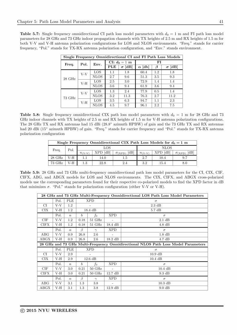
Chapter 5: Path Loss Model Parameters and Analysis 41
Table 5.7: Single frequency omnidirectional CI path loss model parameters with d0 = 1 m and FI path loss modelparameters for 28 GHz and 73 GHz indoor propagation channels with TX heights of 2.5 m and RX heights of 1.5 m forboth V-V and V-H antenna polarization configurations for LOS and NLOS environments. “Freq.” stands for carrierfrequency, “Pol.” stands for TX-RX antenna polarization configuration, and “Env.” stands environment.
Single Frequency Omnidirectional CI and FI Path Loss Models
Freq. Pol. Env.CI: d0 = 1 m FI
PLE σ [dB] α [db] β σ [dB]
28 GHz
V-VLOS 1.1 1.8 60.4 1.2 1.8
NLOS 2.7 9.6 51.3 3.5 9.3
V-HLOS 2.5 3.0 72.9 1.4 1.4
NLOS 3.6 9.4 61.9 3.6 9.4
73 GHz
V-VLOS 1.3 2.4 77.9 0.5 1.4
NLOS 3.2 11.3 76.3 2.7 11.2
V-HLOS 3.5 6.3 94.7 1.1 2.3
NLOS 4.5 9.7 96.1 2.2 7.5
Table 5.8: Single frequency omnidirectional CIX path loss model parameters with d0 = 1 m for 28 GHz and 73GHz indoor channels with TX heights of 2.5 m and RX heights of 1.5 m for V-H antenna polarization configurations.The 28 GHz TX and RX antennas had 15 dBi (28.8◦ azimuth HPBW) of gain and the 73 GHz TX and RX antennashad 20 dBi (15◦ azimuth HPBW) of gain. “Freq.” stands for carrier frequency and “Pol.” stands for TX-RX antennapolarization configuration
Single Frequency Omnidirectional CIX Path Loss Models for d0 = 1 m
Freq. Pol.LOS NLOS
n(V-V) XPD [dB] σ(XPD) [dB] n(V-V) XPD [dB] σ(XPD) [dB]
28 GHz V-H 1.1 14.0 1.5 2.7 10.4 9.7
73 GHz V-H 1.3 22.8 2.4 3.2 15.4 8.0
Table 5.9: 28 GHz and 73 GHz multi-frequency omnidirectional path loss model parameters for the CI, CIX, CIF,CIFX, ABG, and ABGX models for LOS and NLOS environments. The CIX, CIFX, and ABGX cross-polarizedmodels use the corresponding parameters found for their respective co-polarized models to find the XPD factor in dBthat minimizes σ. “Pol.” stands for polarization configuration (either V-V or V-H).
28 GHz and 73 GHz Multi-Frequency Omnidirectional LOS Path Loss Model Parameters
Pol. PLE XPD σ
CI V-V 1.2 - 2.3 dB
CIX V-H 1.2 18.4 dB 5.7 dB
Pol. n b f0 XPD σ
CIF V-V 1.2 0.18 51 GHz - 2.1 dB
CIFX V-H 1.2 0.18 51 GHz 18.4 dB 4.8 dB
Pol. α β γ XPD σ
ABG V-V 0.9 26.8 2.6 - 1.8 dB
ABGX V-H 0.9 26.8 2.6 18.2 dB 4.7 dB
28 GHz and 73 GHz Multi-Frequency Omnidirectional NLOS Path Loss Model Parameters
Pol. PLE XPD σ
CI V-V 2.9 - 10.9 dB
CIX V-H 2.9 12.6 dB 10.4 dB
Pol. n b f0 XPD σ
CIF V-V 3.0 0.21 50 GHz - 10.4 dB
CIFX V-H 3.0 0.21 50 GHz 12.7 dB 9.3 dB
Pol. α β γ XPD σ
ABG V-V 3.1 1.3 3.8 - 10.3 dB
ABGX V-H 3.1 1.3 3.8 12.9 dB 9.0 dB
c© 2015 NYU WIRELESS

42 Chapter 5: Path Loss Model Parameters and Analysis
The FI omnidirectional models at 28 GHz and 73 GHz have intercept α values in LOS environments, that areseveral dB offset from theoretical free space at 1 m at both 28 GHz and 73 GHz. The very low LOS β slopevalue of 0.5 at 73 GHz shows the extreme sensitivity of the FI model and how the model parameters defyphysical interpretation (where a PLE value less than 1 in the CI model implies gain with increasing distance).This illustrates the caution that must be taken to extrapolate the FI model outside of the measurementrange.
The small LOS β slope values may be due to the small sample set of LOS locations. The strength of the CImodel compared to the FI model is that it only requires a single parameter to accurately predict path loss,and models FSPL up until the reference distance d0, giving an accurate physically-based reference anchorpoint for estimating LOS path loss. Choosing d0 = 1 m is convenient and sensible because FSPL existsin the first meter of propagation, before the transmitted wave encounters most walls, ceilings, and floorsthat cause reflections, scattering, or diffraction loss (blockage). If more LOS omnidirectional locations weremeasured, we would expect the FI β slope to converge to the CI PLE values in LOS environments (1.1 and1.3 at 28 GHz and 73 GHz, respectively), as shown in the 28 GHz LOS V-V model displayed in Fig. 5.3a,where the CI PLE and FI β values are within 0.1 of each other.
Some researchers may correctly argue that the two parameter FI model (4.3) reduces the shadow factor(standard deviation) about the mean path loss line compared to the shadow factor found using the singleparameter CI path loss model (4.1). That argument may be true in very sparse measurement data sets, butwhen enough measurements are taken, the standard deviations are generally within a fraction of a dB forboth models as seen in Table 5.7 and [105]. From this study, Table 5.7 shows that their are only three cases(all cross-polarized cases) where the standard deviation is more than 1 dB different between the CI and FIomnidirectional models: the 73 GHz V-H NLOS case, and the 28 GHz and 73 GHz LOS V-H cases, where thestandard deviation is different by 2.2 dB, 1.6 dB and 4.0 dB, respectively, yet we have already established thatthe CIX model with an XPD term in (4.2) is a better estimator of path loss for V-H antenna configurationsthan either the CI or FI model (Compare Table 5.7 and Table 5.8). Furthermore, the CIX model providesnearly identical standard deviations compared to the FI model, where the maximum difference in standarddeviation of both models over all frequencies and environments is 0.5 dB. Important points to consider arethat all models here have rather large standard deviations (8 dB or so), so selecting a simpler path lossmodel that has fewer parameters with less than a dB of difference in standard deviation assures virtuallyidentical modeling accuracy in the face of typical measurement error, physical database error, and cableand calibration fluctuations [105]. Further, in the absence of measured data, the physical foundation ofthe CI family of path loss models allows for extrapolation beyond the 3D T-R separation distances of themeasurements because they are physically-anchored to a known free space (true transmitter power) path lossvalue and distance, whereas the FI models are only valid over the measured 3D T-R separation distances.
A key observation from the omnidirectional path loss data is the pronounced increase in the PLE for 73 GHzcompared to 28 GHz, for any given environment due to the increased loss experienced by signals with smallerwavelengths. The standard deviation also increased at 73 GHz compared to 28 GHz for the omnidirectionalmodels, as seen in Tables 5.7–5.8. Due to a more stringent noise thresholding algorithm used here anddescribed in [105], values in Table 5.7 are slightly different than those presented in [103]. The differencesin the CI, FI, and CIX model standard deviations in Tables 5.7–5.8 are 1 dB or less in a majority of thedifferent environments and scenarios, while the overall standard deviations are much larger (greater than 8dB in NLOS cases).
Multi-frequency omnidirectional path loss model parameters for co- and cross-polarized antennas are givenin Table 5.9. Similar to the directional models, the standard deviations for each omnidirectional multi-frequency model with specific polarizations (CI, CIF, and ABG) are within 1 dB for the corresponding LOSand NLOS environments (σ is between 1.8 dB and 2.3 dB in LOS and between 10.3 dB and 10.9 dB inNLOS for the CI, CIF, and ABG models). The FSPL anchoring point is an advantage in the CI and CIF
c© 2015 NYU WIRELESS
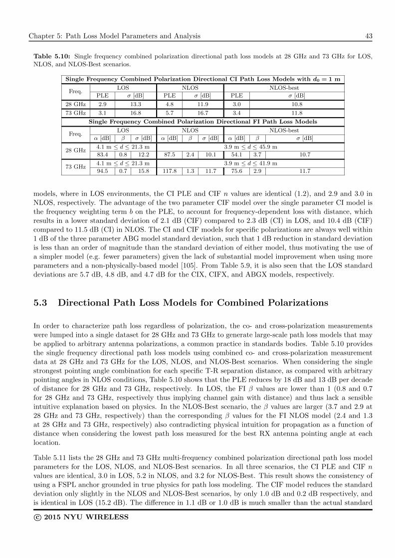
Chapter 5: Path Loss Model Parameters and Analysis 43
Table 5.10: Single frequency combined polarization directional path loss models at 28 GHz and 73 GHz for LOS,NLOS, and NLOS-Best scenarios.
Single Frequency Combined Polarization Directional CI Path Loss Models with d0 = 1 m
Freq.LOS NLOS NLOS-best
PLE σ [dB] PLE σ [dB] PLE σ [dB]
28 GHz 2.9 13.3 4.8 11.9 3.0 10.8
73 GHz 3.1 16.8 5.7 16.7 3.4 11.8
Single Frequency Combined Polarization Directional FI Path Loss Models
Freq.LOS NLOS NLOS-best
α [dB] β σ [dB] α [dB] β σ [dB] α [dB] β σ [dB]
28 GHz4.1 m ≤ d ≤ 21.3 m 3.9 m ≤ d ≤ 45.9 m
83.4 0.8 12.2 87.5 2.4 10.1 54.1 3.7 10.7
73 GHz4.1 m ≤ d ≤ 21.3 m 3.9 m ≤ d ≤ 41.9 m
94.5 0.7 15.8 117.8 1.3 11.7 75.6 2.9 11.7
models, where in LOS environments, the CI PLE and CIF n values are identical (1.2), and 2.9 and 3.0 inNLOS, respectively. The advantage of the two parameter CIF model over the single parameter CI model isthe frequency weighting term b on the PLE, to account for frequency-dependent loss with distance, whichresults in a lower standard deviation of 2.1 dB (CIF) compared to 2.3 dB (CI) in LOS, and 10.4 dB (CIF)compared to 11.5 dB (CI) in NLOS. The CI and CIF models for specific polarizations are always well within1 dB of the three parameter ABG model standard deviation, such that 1 dB reduction in standard deviationis less than an order of magnitude than the standard deviation of either model, thus motivating the use ofa simpler model (e.g. fewer parameters) given the lack of substantial model improvement when using moreparameters and a non-physically-based model [105]. From Table 5.9, it is also seen that the LOS standarddeviations are 5.7 dB, 4.8 dB, and 4.7 dB for the CIX, CIFX, and ABGX models, respectively.
5.3 Directional Path Loss Models for Combined Polarizations
In order to characterize path loss regardless of polarization, the co- and cross-polarization measurementswere lumped into a single dataset for 28 GHz and 73 GHz to generate large-scale path loss models that maybe applied to arbitrary antenna polarizations, a common practice in standards bodies. Table 5.10 providesthe single frequency directional path loss models using combined co- and cross-polarization measurementdata at 28 GHz and 73 GHz for the LOS, NLOS, and NLOS-Best scenarios. When considering the singlestrongest pointing angle combination for each specific T-R separation distance, as compared with arbitrarypointing angles in NLOS conditions, Table 5.10 shows that the PLE reduces by 18 dB and 13 dB per decadeof distance for 28 GHz and 73 GHz, respectively. In LOS, the FI β values are lower than 1 (0.8 and 0.7for 28 GHz and 73 GHz, respectively thus implying channel gain with distance) and thus lack a sensibleintuitive explanation based on physics. In the NLOS-Best scenario, the β values are larger (3.7 and 2.9 at28 GHz and 73 GHz, respectively) than the corresponding β values for the FI NLOS model (2.4 and 1.3at 28 GHz and 73 GHz, respectively) also contradicting physical intuition for propagation as a function ofdistance when considering the lowest path loss measured for the best RX antenna pointing angle at eachlocation.
Table 5.11 lists the 28 GHz and 73 GHz multi-frequency combined polarization directional path loss modelparameters for the LOS, NLOS, and NLOS-Best scenarios. In all three scenarios, the CI PLE and CIF nvalues are identical, 3.0 in LOS, 5.2 in NLOS, and 3.2 for NLOS-Best. This result shows the consistency ofusing a FSPL anchor grounded in true physics for path loss modeling. The CIF model reduces the standarddeviation only slightly in the NLOS and NLOS-Best scenarios, by only 1.0 dB and 0.2 dB respectively, andis identical in LOS (15.2 dB). The difference in 1.1 dB or 1.0 dB is much smaller than the actual standard
c© 2015 NYU WIRELESS

44 Chapter 5: Path Loss Model Parameters and Analysis
1
1020
304050
20
40
60
8060
80
100
120
140
160
180
Distance (m)
Indoor Office 28 GHz and 73 GHz Combined PolarizationDirectional LOS and NLOS CIF Path Loss Models
Frequency (GHz)
Pat
h L
oss
(d
B) 28 GHz LOS
73 GHz LOS28 GHz NLOS73 GHz NLOSCIF
LOS @ 28 GHz
CIFLOS
@ 73 GHz
CIFNLOS
@ 28 GHz
CIFNLOS
@ 73 GHz
CIFLOS
: n = 3.0, b = 0.07, f0 = 51 GHz,
σ = 15.2 dB
CIFNLOS
: n = 5.2, b = 0.21, f0 = 50 GHz,
σ = 14.5 dB
(a) Multi-frequency combined polarization directional CIFLOS and NLOS scatter plot
1
1020
304050
20
40
60
8060
80
100
120
140
160
180
Distance (m)
Indoor Office 28 GHz and 73 GHz Combined PolarizationDirectional LOS and NLOS ABG Path Loss Models
Frequency (GHz)
Pat
h L
oss
(d
B) 28 GHz LOS
73 GHz LOS28 GHz NLOS73 GHz NLOSABG
LOS @ 28 GHz
ABGLOS
@ 73 GHz
ABGNLOS
@ 28 GHz
ABGNLOS
@ 73 GHz
ABGLOS
: α = 0.7, β = 47.1, γ = 2.5,
σ = 14.2 dB
ABGNLOS
: α = 1.9, β = 27.5, γ = 4.5,
σ = 11.0 dB
(b) Multi-frequency combined polarization directionalABG LOS and NLOS scatter plot
Fig. 5.4: 28 GHz and 73 GHz multi-frequency combined polarization CIF and ABG directional path loss models forLOS and NLOS environments. Red circles represent 28 GHz LOS directional path loss values, green squares represent73 GHz LOS directional path loss values, solid gray circles represent 28 GHz NLOS directional path loss values, andsolid blue squares represent 73 GHz NLOS directional path loss values for (a) CIF Model; (b) ABG Model.
deviation value of 15.5 dB (CI-NLOS) and 14.5 dB (CIF-NLOS) as shown in Table 5.11. For the ABGmodel, the α and β terms are seen to vary over a wide range of values that do not provide intuitive sense.Table 5.11 does show that the ABG model for LOS, NLOS, and NLOS-best has lower standard deviationthan both the CI and CIF models, but the reduction is so small (a few dB to a fraction of a dB) comparedto the overall standard deviation values which are all greater than 11 dB. Figs 5.4a and 5.4b show theLOS and NLOS CIF and ABG directional path loss models for combined polarizations. Note that the CIFmodel standard deviation is within 0.4 dB of the ABG model in the NLOS-Best scenario. For the NLOSarbitrary pointing angle case, the standard deviation for the ABG model is 3.5 dB smaller than the CIFmodel, reducing it from 14.5 dB to 11 dB through the use of three modeling parameters, but Table 5.11shows that the ABG model parameters vary over a wide range without intuition of the physics, and in theother cases (LOS and NLOS-Best) the differences in standard deviation between the CIF and ABG modelsare less than a dB, less than an order of magnitude of standard deviation values of all models, and certainlyin the measurement noise.
5.4 Omnidirectional Path Loss Models for Combined Polarizations
Using the synthesized omnidirectional path loss values described here, and given in Appendix B, omnidirec-tional path loss models were computed for single and multi-frequency cases at 28 GHz and 73 GHz with theco- and cross-polarized measurements lumped into a common dataset. Table 5.12 provides single frequencypath loss model parameters at 28 GHz and 73 GHz and Figs. 5.5a and 5.5b display the corresponding 28 GHzand 73 GHz scatter plots. It is apparent that the 28 GHz and 73 GHz NLOS CI model standard deviationis within 1 dB of the NLOS FI model, well within measurement error, and less than an order of magnitudethan the actual standard deviations, where the CI model requires only one parameter and uses a physicallybased FSPL anchoring point. The FI model 73 GHz LOS β slope value indicates channel amplification withdistance (0.8). The FI model is limited as it is only valid over the measurement range of the data, which is
c© 2015 NYU WIRELESS
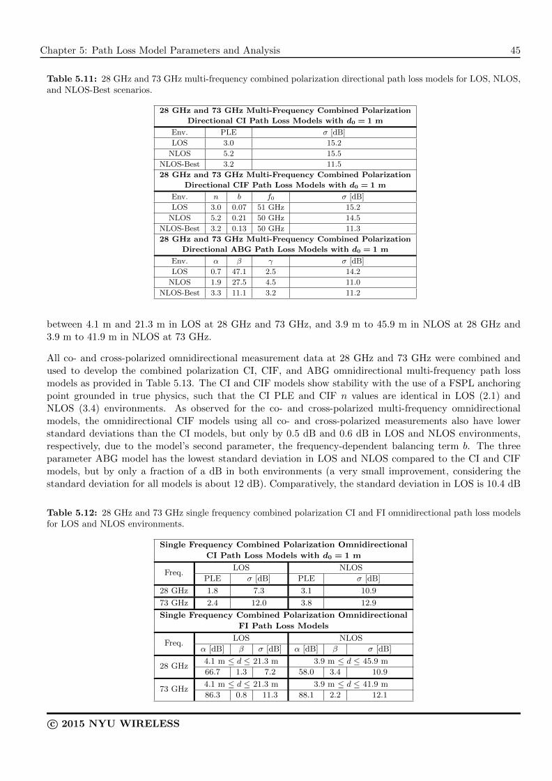
Chapter 5: Path Loss Model Parameters and Analysis 45
Table 5.11: 28 GHz and 73 GHz multi-frequency combined polarization directional path loss models for LOS, NLOS,and NLOS-Best scenarios.
28 GHz and 73 GHz Multi-Frequency Combined Polarization
Directional CI Path Loss Models with d0 = 1 m
Env. PLE σ [dB]
LOS 3.0 15.2
NLOS 5.2 15.5
NLOS-Best 3.2 11.5
28 GHz and 73 GHz Multi-Frequency Combined Polarization
Directional CIF Path Loss Models with d0 = 1 m
Env. n b f0 σ [dB]
LOS 3.0 0.07 51 GHz 15.2
NLOS 5.2 0.21 50 GHz 14.5
NLOS-Best 3.2 0.13 50 GHz 11.3
28 GHz and 73 GHz Multi-Frequency Combined Polarization
Directional ABG Path Loss Models with d0 = 1 m
Env. α β γ σ [dB]
LOS 0.7 47.1 2.5 14.2
NLOS 1.9 27.5 4.5 11.0
NLOS-Best 3.3 11.1 3.2 11.2
between 4.1 m and 21.3 m in LOS at 28 GHz and 73 GHz, and 3.9 m to 45.9 m in NLOS at 28 GHz and3.9 m to 41.9 m in NLOS at 73 GHz.
All co- and cross-polarized omnidirectional measurement data at 28 GHz and 73 GHz were combined andused to develop the combined polarization CI, CIF, and ABG omnidirectional multi-frequency path lossmodels as provided in Table 5.13. The CI and CIF models show stability with the use of a FSPL anchoringpoint grounded in true physics, such that the CI PLE and CIF n values are identical in LOS (2.1) andNLOS (3.4) environments. As observed for the co- and cross-polarized multi-frequency omnidirectionalmodels, the omnidirectional CIF models using all co- and cross-polarized measurements also have lowerstandard deviations than the CI models, but only by 0.5 dB and 0.6 dB in LOS and NLOS environments,respectively, due to the model’s second parameter, the frequency-dependent balancing term b. The threeparameter ABG model has the lowest standard deviation in LOS and NLOS compared to the CI and CIFmodels, but by only a fraction of a dB in both environments (a very small improvement, considering thestandard deviation for all models is about 12 dB). Comparatively, the standard deviation in LOS is 10.4 dB
Table 5.12: 28 GHz and 73 GHz single frequency combined polarization CI and FI omnidirectional path loss modelsfor LOS and NLOS environments.
Single Frequency Combined Polarization Omnidirectional
CI Path Loss Models with d0 = 1 m
Freq.LOS NLOS
PLE σ [dB] PLE σ [dB]
28 GHz 1.8 7.3 3.1 10.9
73 GHz 2.4 12.0 3.8 12.9
Single Frequency Combined Polarization Omnidirectional
FI Path Loss Models
Freq.LOS NLOS
α [dB] β σ [dB] α [dB] β σ [dB]
28 GHz4.1 m ≤ d ≤ 21.3 m 3.9 m ≤ d ≤ 45.9 m
66.7 1.3 7.2 58.0 3.4 10.9
73 GHz4.1 m ≤ d ≤ 21.3 m 3.9 m ≤ d ≤ 41.9 m
86.3 0.8 11.3 88.1 2.2 12.1
c© 2015 NYU WIRELESS

46 Chapter 5: Path Loss Model Parameters and Analysis
Table 5.13: 28 GHz and 73 GHz multi-frequency combined polarization CI, CIF, and ABG omnidirectional path lossmodels for LOS and NLOS environments.
28 GHz and 73 GHz Multi-Frequency Combined Polarization
Omnidirectional CI Path Loss Models with d0 = 1 m
Env. PLE σ [dB]
LOS 2.1 10.4
NLOS 3.4 12.5
28 GHz and 73 GHz Multi-Frequency Combined Polarization
Omnidirectional CIF Path Loss Models with d0 = 1 m
Env. n b f0 σ [dB]
LOS 2.1 0.32 51 GHz 9.9
NLOS 3.4 0.22 49 GHz 11.9
28 GHz and 73 GHz Multi-Frequency Combined Polarization
Omnidirectional ABG Path Loss Models with d0 = 1 m
Env. α β γ σ [dB]
LOS 1.1 17.7 3.5 9.5
NLOS 2.9 4.5 4.1 11.6
1 10 20 30 40 5060
80
100
120
140
n = 1
n = 2
n = 3
n = 4
T−R Separation (meters)
Pat
h Lo
ss (
dB)
28 GHz Indoor Combined Polarization Omnidirectional Path Loss Modelswith TX Height: 2.5 m and RX Height: 1.5 m
LOSNLOSn
LOS = 1.8, σ
LOS = 7.3 dB
nNLOS
= 3.1, σNLOS
= 10.9 dB
LOS (α , β, σ), = (66.7 dB, 1.3, 7.2 dB)NLOS (α , β, σ), = (58.0 dB, 3.4, 10.9 dB)
(a) 28 GHz omnidirectional combined polarization pathloss
1 10 20 30 40 50
80
100
120
140
n = 1
n = 2
n = 3
n = 4
T−R Separation (meters)
Pat
h Lo
ss (
dB)
73 GHz Indoor Combined Polarization Omnidirectional Path Loss Modelswith TX Height: 2.5 m and RX Height: 1.5 m
LOSNLOSn
LOS = 2.4, σ
LOS = 12.0 dB
nNLOS
= 3.8, σNLOS
= 12.9 dB
LOS (α, β, σ), = (86.3 dB, 0.8, 11.3 dB)NLOS (α, β, σ), = (88.1 dB, 2.2, 12.1 dB)
(b) 73 GHz omnidirectional combined polarization pathloss
Fig. 5.5: 28 GHz and 73 GHz single frequency combined polarization CI and FI omnidirectional path loss modelsfor LOS and NLOS environments. Gray circles represent LOS omnidirectional path loss values and solid blue squaresrepresent NLOS omnidirectional path loss values for (a) 28 GHz; (b) 73 GHz.
for CI, 9.9 dB for CIF, and 9.5 dB for the ABG model, not a large difference for standard deviations that arealready greater than 9 dB. Furthermore, the standard deviation in NLOS is 12.5 dB for CI, 11.9 dB for CIF,and 11.6 dB for the ABG model, also within measurement errors and typical cable loss variations or gain driftin typical measurements, and not a vast difference for already large standard deviations. Figs. 5.6a and 5.6bshow the 3D scatter plots of omnidirectional LOS and NLOS path loss values and the corresponding CIFand ABG path loss models, where the CIF model is anchored by FSPL at 1 m. Both figures show a similartrend as path loss increases with frequency. The combined polarization omnidirectional path loss modelsgiven in Tables 5.12 and 5.13 also show comparable standard deviations in LOS and NLOS environmentsbetween the CI and FI single frequency models and the CI, CIF, and ABG multi-frequency models, wheredifferences in standard deviations are less than an order of magnitude of the standard deviation, and lessthan or equal to 1 dB in all cases.
c© 2015 NYU WIRELESS

Chapter 5: Path Loss Model Parameters and Analysis 47
1
1020
304050
20
40
60
8060
80
100
120
140
160
Distance (m)
Indoor Office 28 GHz and 73 GHz Combined PolarizationOmnidirectional LOS and NLOS CIF Path Loss Models
Frequency (GHz)
Pat
h L
oss
(d
B) 28 GHz LOS
73 GHz LOS28 GHz NLOS73 GHz NLOSCIF
LOS @ 28 GHz
CIFLOS
@ 73 GHz
CIFNLOS
@ 28 GHz
CIFNLOS
@ 73 GHz
CIFLOS
: n = 2.1, b = 0.32, f0 = 51 GHz,
σ = 9.9 dB
CIFNLOS
: n = 3.4, b = 0.22, f0 = 49 GHz,
σ = 11.9 dB
(a) Multi-frequency combined polarization omnidirec-tional CIF LOS and NLOS path loss
1
1020
304050
20
40
60
8060
80
100
120
140
160
Distance (m)
Indoor Office 28 GHz and 73 GHz Combined PolarizationOmnidirectional LOS and NLOS ABG Path Loss Models
Frequency (GHz)
Pat
h L
oss
(d
B) 28 GHz LOS
73 GHz LOS28 GHz NLOS73 GHz NLOSABG
LOS @ 28 GHz
ABGLOS
@ 73 GHz
ABGNLOS
@ 28 GHz
ABGNLOS
@ 73 GHz
ABGLOS
: α = 1.1, β = 17.7, γ = 3.5,
σ = 9.5 dB
ABGNLOS
: α = 2.9, β = 4.5, γ = 4.1,
σ = 11.6 dB
(b) Multi-frequency combined polarization omnidirec-tional ABG LOS and NLOS path loss
Fig. 5.6: 28 GHz and 73 GHz multi-frequency combined polarization CIF and ABG omnidirectional path loss modelfor LOS and NLOS environments. Gray circles represent 28 GHz LOS omnidirectional path loss values, blue squaresrepresent 73 GHz LOS omnidirectional path loss values, solid gray circles represent 28 GHz NLOS omnidirectionalpath loss values, and solid blue squares represent 73 GHz NLOS omnidirectional path loss values for (a) CIF Model;(b) ABG Model.
From the large-scale path loss models and parameters shown above, it is apparent that the single frequencyCI model does an excellent job in predicting indoor path loss at mmWave frequencies by using a singleparameter. For multiple-frequency omnidirectional modeling, it is clear that indoor channels offer greaterloss with distance at higher frequencies. The work above shows that the two parameter CIF model retainsa physical link to the physics of propagation while reducing the standard deviation as compared to the CImodel. The three parameter ABG model can typically obtain a fraction of a dB to a dB or two less standarddeviation but at the expense of an additional parameter model and a lack of physical basis. Thus, theCIF model appears to be a good candidate for indoor large-scale path loss modeling over a wide range ofmmWave frequencies.
c© 2015 NYU WIRELESS

This page is intentionally left blank.

Chapter 6
Time Dispersion Properties
6.1 MmWave Indoor Time Dispersion Properties
The time dispersion properties of wideband channels are generally characterized by RMS delay spread,as it is a good measure of the multipath time dispersion and coherence bandwidth nature of multipathchannels, and an indication of the potential severity of intersymbol interference, depending on the signal’sbandwidth [49, 132, 133]. To build power-efficient mmWave mobile communications systems with simpleequalization, it was recently postulated that there could be advantages in searching for particular beampointing directions that offer both minimum path loss and minimum multipath delay spread [120]. Physicallayer design is often dictated by channel RMS delay spread and time dispersion characteristics, and analysisof such properties can provide valuable information for the design of indoor mmWave communicationssystems. All RMS delay spread and temporal statistics presented in this section are for typical LOS andNLOS environments.
The RMS delay spread is defined as the square root of the second moment of a PDP [49]:
στ =
√τ2 − (τ̄)2 (6.1)
where,
τ̄ =
∑k P (τk)τk∑k P (τk)
(6.2)
τ2 =
∑k P (τk)τk
2∑k P (τk)
(6.3)
In Eqs. (6.1)-(6.3), στ is the RMS delay spread, P (τk) is the received power (in mW) at the delay bincentered at τk, τ̄ is the mean excess delay which is the first moment of a PDP, and τ2 is the second centralmoment of a PDP. We captured a PDP at each unique antenna pointing angle between the TX and RXin the azimuth and elevation planes, for all measured TX and RX pointing angles between each TX-RXlocation combination.
6.1.1 Multipath Time Dispersion Statistics for Co- or Cross-Polarized Antennas
Figs. 6.1a and 6.1b show the cumulative distribution functions (CDF) for the RMS delay spreads of thePDPs measured over all pointing angles at 28 GHz for V-V and V-H antenna polarization configurations,respectively. Both figures show that 90% of the measured RMS delay spreads in both LOS and NLOS

50 Chapter 6: Time Dispersion Properties
0 10 20 30 40 50 60 700
0.1
0.2
0.3
0.4
0.5
0.6
0.7
0.8
0.9
1CDF of 28 GHz VV Indoor RMS Delay Spread for LOS and NLOS
RMS Delay Spread (ns)
Pro
babi
lity
RM
S D
elay
S
prea
d <
Abs
ciss
a
E[28 GHz(LOS)σt] = 17.3 ns
E[28 GHz(NLOS)σt] = 17.7 ns
E[Strongest − 28 GHz(LOS) σt] = 4.1 ns
E[Strongest − 28 GHz(NLOS) σt] = 13.4 ns
Elevation HPBW = 30 ° @ 28 GHz
Azimuth HPBW = 28.8 ° @ 28 GHz
28 GHz Indoor LOS28 GHz Indoor NLOSStrongest − 28 GHz Indoor LOSStrongest − 28 GHz Indoor NLOS
(a) 28 GHz V-V indoor directional RMS delay spread
0 10 20 30 40 50 60 700
0.1
0.2
0.3
0.4
0.5
0.6
0.7
0.8
0.9
1CDF of 28 GHz VH Indoor RMS Delay Spread for LOS and NLOS
RMS Delay Spread (ns)
Pro
babi
lity
RM
S D
elay
S
prea
d <
Abs
ciss
a
E[28 GHz(LOS)σt] = 17.2 ns
E[28 GHz(NLOS)σt] = 18 ns
E[Strongest − 28 GHz(LOS) σt] = 7.3 ns
E[Strongest − 28 GHz(NLOS) σt] = 13.2 ns
Elevation HPBW = 30 ° @ 28 GHz
Azimuth HPBW = 28.8 ° @ 28 GHz
28 GHz Indoor LOS28 GHz Indoor NLOSStrongest − 28 GHz Indoor LOSStrongest − 28 GHz Indoor NLOS
(b) 28 GHz V-H indoor directional RMS delay spread
0 10 20 30 40 50 60 700
0.1
0.2
0.3
0.4
0.5
0.6
0.7
0.8
0.9
1CDF of 73 GHz VV Indoor RMS Delay Spread for LOS and NLOS
RMS Delay Spread (ns)
Pro
babi
lity
RM
S D
elay
S
prea
d <
Abs
ciss
a
E[73 GHz(LOS)σt] = 12.8 ns
E[73 GHz(NLOS)σt] = 12.3 ns
E[Strongest − 73 GHz(LOS) σt] = 3.6 ns
E[Strongest − 73 GHz(NLOS) σt] = 11.3 ns
Elevation HPBW = 15 ° @ 73 GHz
Azimuth HPBW = 15 ° @ 73 GHz
73 GHz Indoor LOS73 GHz Indoor NLOSStrongest − 73 GHz Indoor LOSStrongest − 73 GHz Indoor NLOS
(c) 73 GHz V-V indoor directional RMS delay spread
0 10 20 30 40 50 60 700
0.1
0.2
0.3
0.4
0.5
0.6
0.7
0.8
0.9
1CDF of 73 GHz VH Indoor RMS Delay Spread for LOS and NLOS
RMS Delay Spread (ns)
Pro
babi
lity
RM
S D
elay
S
prea
d <
Abs
ciss
a
E[73 GHz(LOS)σt] = 11.4 ns
E[73 GHz(NLOS)σt] = 8.4 ns
E[Strongest − 73 GHz(LOS) σt] = 7 ns
E[Strongest − 73 GHz(NLOS) σt] = 12.5 ns
Elevation HPBW = 15 ° @ 73 GHz
Azimuth HPBW = 15 ° @ 73 GHz
73 GHz Indoor LOS73 GHz Indoor NLOSStrongest − 73 GHz Indoor LOSStrongest − 73 GHz Indoor NLOS
(d) 73 GHz V-H indoor directional RMS delay spread
Fig. 6.1: 28 GHz and 73 GHz arbitrary pointing angle (directional) RMS delay spread CDFs for TX antenna heightsof 2.5 m RX antenna heights of 1.5 m in a typical indoor office environment for co- and cross-polarized TX and RXantennas in LOS and NLOS environments. The T-R separation distances ranged from 3.9 m to 45.9 m. (a) 28 GHzV-V; (b) 28 GHz V-H; (c) 73 GHz V-V; and (d) 73 GHz V-H.
c© 2015 NYU WIRELESS

Chapter 6: Time Dispersion Properties 51
environments are less than 40 ns for all measured arbitrary pointing angles. The NLOS locations weregenerally found to have greater RMS delay spreads than LOS locations, since obstructions in NLOS locationsblocked or severely attenuated the direct path, causing multipath to arrive at the receiver over a largerpropagation time interval. In LOS environments, the LOS component was much stronger than reflectedor scattered paths, leading to lower RMS delay spreads. Similar trends were observed in propagationmeasurements below 6 GHz, conducted by Hashemi et al. in two office environments [133]. The mean RMSdelay spread was smaller in LOS environments (where the direct path was dominant) compared to NLOSenvironments (where the direct path was obstructed). Similar RMS delay spread statistics at 60 GHz werereported by Geng et al., where RMS delay spreads in a NLOS hall were larger than in either a LOS hall orcorridor [74].
The measured mean RMS delay spreads at 28 GHz are between 17 ns and 18 ns in all environments andpolarization combinations (as summarized in Table 6.1), which in general are larger than the mean RMSdelay spreads between 8 ns and 13 ns at 73 GHz. Similar results were reported by Yang et al. where themean RMS delay spreads at 58 GHz (8 ns to 14 ns) were about 50% lower than those at 2.25 GHz (20 ns to28 ns) due to high penetration loss caused by walls, such that multipath components observed at 58 GHzcame mostly from reflected waves confined to the room, while the reflected waves from neighboring roomsat 2.25 GHz had significantly longer delays [134].
The results reported in Table 6.1 and displayed in Fig. 6.1 show that the minimum measured RMS delayspreads are all lower than 1 ns, while the maximum delay spread values observed are all greater than 100ns, regardless of frequency or environment. Maximum RMS delay spreads were measured to be 98 ns at58 GHz [68], between 100 ns and 150 ns at 1.5 GHz [18], and up to 250 ns at 850 MHz [135]. At 28 GHzand 73 GHz the maximum measured RMS delay spreads in LOS environments are smaller than in NLOSenvironments for most cases, with the only exception for the 73 GHz V-H antenna polarization scenario,where the maximum RMS delay in a NLOS environment is larger than that in a LOS environment (21.6 nsgreater), as noticed in Table 6.1 and Fig. 6.1. Additionally, standard deviations of RMS delay spreads inLOS and NLOS environments at both frequencies are less than 18 ns. There was no clear trend observedbetween the minimum RMS delay spreads and standard deviations of RMS delay spreads in relation toenvironment, polarization, and frequency.
We also studied the RMS delay spreads when considering the single best unique antenna pointing anglesbetween the TX and RX locations that resulted in the strongest received power, for each TX-RX locationcombination measured. For all LOS and NLOS locations measured, the CDF of the RMS delay spreads forthe angles with the strongest received power (lowest path loss) are also provided in the subfigures in Fig. 6.1.For both 28 GHz and 73 GHz, and for the co- and cross-polarized antenna configurations, the mean RMSdelay spreads when considering the single strongest pointing angles are less as compared to the mean RMSdelay spreads over all unique antenna pointing angles measured for all locations, except for 73 GHz V-HNLOS. This is particularly true for LOS environments, where Fig. 6.1 shows that the strongest beams offermuch smaller RMS delay spread than arbitrary pointing beams, although the difference is not as great forNLOS channels. For cross-polarized NLOS channels, however, the best beam can sometimes increase themultipath dispersion. As shown in Table 6.1 and Fig. 6.1, the strongest beams in NLOS locations resulted ingreater standard deviations than in LOS locations, which is not observed when considering arbitrary pointingangles. Table 6.1 shows that the minimum values of RMS delay spreads when considering the best beam arein general within 4 ns regardless of frequency, environment, and antenna polarization, indicating that thebest beam can simultaneously minimize path loss and RMS delay spread. These observations indicate theopportunity to minimize multipath time dispersion with high gain, narrowbeam, directional, co-polarizedantennas for indoor mmWave communications systems when exploiting the strongest pointing angle beamsbetween the TX and RX.
Figs. 6.1c and 6.1d show similar RMS delay spread CDF curves at 73 GHz for both V-V and V-H antennapolarization configurations. The figures indicate that 90% of RMS delay spreads in both LOS and NLOS
c© 2015 NYU WIRELESS

52 Chapter 6: Time Dispersion Properties
indoor environments are less than 30 ns. Little difference in RMS delay spread is noticed between LOS andNLOS locations for both V-V and V-H antenna configurations.
At both 28 GHz and 73 GHz, the mean RMS delay spreads were significantly reduced when considering thesingle strongest co-polarized pointing angle combinations between the TX and RX antennas, where in V-VLOS cases the mean RMS delay spreads were reduced from 17.3 ns to 4.1 ns, and from 12.8 ns to 3.6 ns, for28 GHz and 73 GHz respectively. Somewhat smaller reductions in RMS delay spreads where seen in NLOSfor the V-V case, where the mean RMS delay spreads were reduced from 17.7 ns to 13.4 ns, and from 12.3ns to 11.3 ns, for 28 GHz and 73 GHz, respectively, when considering the strongest pointing angles. Thesmaller RMS delay spreads are due to the strongest received power angle combinations containing a mainLOS component and very weak multipath at large excess delays (or none at all). The largest difference inmean RMS delay spread for co-polarized antennas when comparing arbitrary pointing angles to the strongestpointing angles is in the LOS environment, where beamforming and beam steering algorithms [136, 137] willbe useful in reducing RMS delay spread by searching for the strongest received power pointing angles. Asseen in Table 6.1, the V-H scenario at 28 GHz was very similar to the V-V case with mean RMS delayspreads reduced by 9.9 ns and 1.0 ns in LOS and NLOS respectively; however, 73 GHz mean RMS delayspreads reduced by 4.4 ns in LOS and increased by 4.1 ns in NLOS for the V-H case.
In all cases for the 28 GHz and 73 GHz measurements, the cross-polarized antenna RMS delay spreads werelarger than co-polarized antenna RMS delay spreads (see Table 6.1), likely a result of additional energycaptured based on wave de-polarization from the TX to RX in the indoor mmWave environment, and wasalso noticed in [22, 24, 107] where cross-polarized omnidirectional antennas experienced 3-4 ns larger meanand maximum RMS delay spreads compared to co-polarized antennas.
Table 6.1 summarizes the mean, standard deviation, minimum, and maximum measured RMS delay spreadstatistics calculated from the 28 GHz and 73 GHz measurements for co- and cross-polarized antenna con-figurations in LOS and NLOS environments. Compared to 28 GHz, the 73 GHz band had smaller observedRMS delay spreads, similar to results reported in [138] when comparing RMS delay spreads of 2 GHz, 5GHz, and 17 GHz. The time dispersion values given in Table 6.1 are marginally different than those in [103]as a result of a newer more stringent noise thresholding method described in [105].
6.1.2 Multipath Time Dispersion Statistics for Combined-Polarized Antennas
Time dispersion characteristics are also important for modeling applications that will employ arbitraryantenna polarization configurations such as mobile handsets that are constantly changing orientations.Figs. 6.2a and 6.2b show the CDFs for the RMS delay spreads for combined polarization measurementsat 28 GHz and 73 GHz, respectively, for PDPs measured over all arbitrary pointing angles and also for thesingle strongest pointing angles for each TX-RX location combination. Table 6.2 summarizes the mean RMSdelay spreads from the figures and includes the standard deviation, minimum, and maximum measured RMSdelay spread statistics calculated at 28 GHz and 73 GHz for combined antenna polarizations for LOS andNLOS environments.
Figs. 6.2a and 6.2b indicate that 90% of RMS delay spreads for combined antenna polarizations, regardlessof environment, are less than 35 ns and 30 ns at 28 GHz and 73 GHz, respectively. From Table 6.1 andTable 6.2, there is no distinguishable difference between co-polarization (V-V) and combined polarizationin the RMS delay spread statistics. The RMS delay spread statistics at 28 GHz are, in general, slightlygreater than the corresponding statistics at 73 GHz. The measured mean RMS delay spreads for combinedpolarizations at 28 GHz are 17.2 ns (LOS) and 17.8 ns (NLOS), and are larger than the mean RMS delayspreads of 12.1 ns (LOS) and 10.7 ns (NLOS) at 73 GHz. Irrespective of frequency and environment, theminimum RMS delay spreads are all less then 2 ns and the maximum RMS delay spreads are all less than
c© 2015 NYU WIRELESS

Chapter 6: Time Dispersion Properties 53
Table 6.1: Comparison of mean, standard deviation, and maximum RMS delay spreads at 28 GHz and 73 GHz forV-V and V-H antenna polarization combinations in LOS and NLOS indoor propagation environments. “Ant. Pol.”means TX-RX antenna polarization and “Env.” indicates the environment type of the RX locations.
RMS Delay Spreads Over All Arbitrary Angles
Ant.Env.
28 GHz
Pol. µ (ns) σ (ns) Min. (ns) Max. (ns)
V-V
LOS 17.3 18.0 0.7 134.4
NLOS 17.7 13.8 0.6 198.5
LOS-Best 4.1 1.6 1.6 6.1
NLOS-Best 13.4 13.1 0.9 47.9
V-H
LOS 17.2 14.5 0.9 126.4
NLOS 18.0 10.9 0.6 128.1
LOS-Best 7.3 3.5 4.2 14.6
NLOS-Best 13.2 10.8 3.5 55.7
Ant.Env.
73 GHz
Pol. µ (ns) σ (ns) Min. (ns) Max. (ns)
V-V
LOS 12.8 16.9 0.6 101.9
NLOS 12.3 14.2 0.5 142.0
LOS-Best 3.6 1.5 0.8 5.1
NLOS-Best 11.3 14.4 3.7 73.4
V-H
LOS 11.4 17.5 0.5 143.8
NLOS 8.4 10.6 0.5 122.2
LOS-Best 7.0 10.9 0.8 37.7
NLOS-Best 12.5 22.5 2.2 122.2
Table 6.2: Comparison of mean, standard deviation, and maximum RMS delay spreads at 28 GHz and 73 GHz forcombined antenna polarizations in LOS and NLOS indoor propagation environments. “Env.” indicates the environmenttype of the RX locations.
RMS Delay Spreads Over All Arbitrary Angles
For Combined Polarizations
Env.28 GHz
µ (ns) σ (ns) Min. (ns) Max. (ns)
LOS 17.2 16.4 0.7 134.4
NLOS 17.8 12.5 0.6 198.5
LOS-Best 4.1 1.6 1.6 6.1
NLOS-Best 13.4 13.1 0.9 47.9
Env.73 GHz
µ (ns) σ (ns) Min. (ns) Max. (ns)
LOS 12.1 17.2 0.5 143.8
NLOS 10.7 13.0 0.5 142.0
LOS-Best 3.6 1.5 0.8 5.1
NLOS-Best 11.3 14.4 3.7 73.4
c© 2015 NYU WIRELESS

54 Chapter 6: Time Dispersion Properties
0 10 20 30 40 50 60 700
0.2
0.4
0.6
0.8
1
CDF of 28 GHz Combined Polarization Indoor OfficeRMS Delay Spread for LOS and NLOS
RMS Delay Spread (ns)
Pro
babi
lity
RM
S D
elay
S
prea
d <
Abs
ciss
a
E[28 GHz(LOS)σt] = 17.2 ns
E[28 GHz(NLOS)σt] = 17.8 ns
E[Strongest − 28 GHz(LOS) σt] = 4.1 ns
E[Strongest − 28 GHz(NLOS) σt] = 13.4 ns
Elevation HPBW = 30 ° @ 28 GHz
Azimuth HPBW = 28.8 ° @ 28 GHz
28 GHz Indoor LOS28 GHz Indoor NLOSStrongest − 28 GHz Indoor LOSStrongest − 28 GHz Indoor NLOS
(a) 28 GHz combined polarization indoor directional RMSdelay spread
0 10 20 30 40 50 60 700
0.2
0.4
0.6
0.8
1
CDF of 73 GHz Combined Polarization Indoor OfficeRMS Delay Spread for LOS and NLOS
RMS Delay Spread (ns)
Pro
babi
lity
RM
S D
elay
S
prea
d <
Abs
ciss
a
E[73 GHz(LOS)σt] = 12.1 ns
E[73 GHz(NLOS)σt] = 10.7 ns
E[Strongest − 73 GHz(LOS) σt] = 3.6 ns
E[Strongest − 73 GHz(NLOS) σt] = 11.3 ns
Elevation HPBW = 15 ° @ 73 GHz
Azimuth HPBW = 15 ° @ 73 GHz
73 GHz Indoor LOS73 GHz Indoor NLOSStrongest − 73 GHz Indoor LOSStrongest − 73 GHz Indoor NLOS
(b) 73 GHz combined polarization indoor directional RMSdelay spread
Fig. 6.2: 28 GHz and 73 GHz arbitrary pointing angle (directional) combined polarization RMS delay spread CDFsfor TX antenna heights of 2.5 m RX antenna heights of 1.5 m in a typical indoor office environment for LOS andNLOS scenarios. The T-R separation distances ranged from 3.9 m to 45.9 m. (a) 28 GHz combined polarization; (b)73 GHz combined polarization.
200 ns. A majority of standard deviations of RMS delay spread are around 15 ns. The minimum valueand standard deviation of RMS delay spreads show no clear dependence on environment, polarization, andfrequency.
Similar to statistics for separate polarizations, the RMS delay spreads are lower when only considering thesingle strongest antenna pointing orientation between the TX and RX at 28 GHz and 73 GHz, most notablywhere Table 6.2 and Fig. 6.2 shows in LOS environments that the mean RMS delay spread reduces from17.2 ns to 4.1 ns at 28 GHz (in LOS) and from 12.1 ns to 3.6 ns at 73 GHz (in LOS). From Table 6.2 it isapparent that the V-V antenna polarization corresponds to the maximum observed RMS delay spreads at28 GHz in LOS (134.4 ns) and NLOS (198.5 ns) environments for combined polarizations (as observed inTable 6.1). The same observation is made at 73 GHz in NLOS (142.0 ns), however, in the LOS case at 73GHz, the V-H antenna polarization in LOS (143.8 ns) corresponds to the maximum observed RMS delayspread for combined antenna polarizations.
Work in [120] suggests a simple algorithm to find the best beam directions that can simultaneously minimizeboth RMS delay spread and path loss (finding the best paths that simultaneously have both strong SNRand very small multipath time dispersion). By selecting a beam with both low RMS delay spread and lowpath loss, relatively high SNR can be achieved at the RX using directional antennas without complicatedequalization, meaning that low latency single carrier (wideband) modulations may be a viable candidate forfuture mmWave wireless communications systems [131]. The measured values presented in Tables 6.1–6.2and Figs. 6.1 and 6.2 give insight to the range of multipath channel parameters for arbitrary pointing co-,cross-, or combined-polarized antennas, as well as for the best TX and RX antenna pointing angles thatresult in the lowest path loss/link attenuation.
c© 2015 NYU WIRELESS

Chapter 7
Conclusion
This report provides the world’s first comprehensive study of indoor channels at 28 GHz and 73 GHzusing different antenna polarizations and combined polarizations to generate large-scale path loss modelsand time delay spreads for the development of 5G standards at 28 GHz and 73 GHz. Directional andomnidirectional path loss models and directional multipath RMS delay spread values are presented, yieldinginsight into mmWave indoor office propagation characteristics. Extensive analysis shows that for mmWaveindoor channels, large-scale path loss over distance and frequency may be modeled with virtually no sacrificein accuracy by using simple close-in (CI) free space reference distance models with just one or two parametersthat ensure a physical tie to the transmitter power, rather than using existing 3GPP and WINNER floatingintercept (FI) models that have no tie to the transmitted power, lack intuition, and require more modelingparameters. The closed-form expressions for optimizing existing and newly proposed large-scale path lossmodel parameters are given in Appendix A, the raw omnidirectional data used to create the large-scale pathloss models in this report are tabulated in Appendix B, and standard deviations of each large-scale path lossmodel are tabulated for side-by-side comparison in Appendix C.
Single frequency directional path loss models were provided using the 1 m close-in free space referencedistance (CI), close-in reference distance with XPD factor (CIX), and floating-intercept (FI) forms. The CIpath loss models showed that for co-polarized antennas, constructive interference due to waveguiding andreflections resulted in nearly identical LOS PLEs of 1.7 and 1.6 for 28 GHz and 73 GHz, respectively, smallerthan theoretical FSPL (n = 2), suggesting that LOS PLEs are independent of frequency. Path loss observedin NLOS environments had much greater attenuation (44 dB (n = 4.4) and 53 dB (n = 5.3) per decade ofdistance for 28 GHz and 73 GHz, respectively) than in LOS environments; however, the high attenuationwas significantly reduced (resulting in n = 3.0 at 28 GHz and n = 3.4 at 73 GHz), when considering thebest TX and RX antenna pointing angles that resulted in the maximum received power at each measuredlocation. The shadowing factor increased from 28 GHz to 73 GHz (2.5 dB to 3.2 dB in LOS, and 11.6 dB to15.7 dB in NLOS), indicating more variability in large-scale shadowing at higher mmWave frequencies, mostlikely due to increased diffuse scattering, greater diffraction loss, and weaker reflections. The directionalPLEs for the V-H antenna polarization configurations indicated significant de-polarization in NLOS indoorenvironments at both 28 GHz and 73 GHz. For LOS channels, large directional XPD factors of 24.7 dBand 31.4 dB were found for V-H scenarios at 28 GHz and 73 GHz, respectively, and showed that there waslarge isolation between co- and cross-polarized transmission when using high-gain directional horn antennas.Larger fluctuations in received signal strength about the distance-dependent mean path loss were observedat 73 GHz in NLOS environments for cross-polarized directional antennas (15.9 dB) compared to 28 GHzcross-polarized directional antennas (10.9 dB). The CIX model was shown to be a useful and simple pathloss model for cross-polarized antenna systems, and was shown to improve (reduce) the standard deviationcompared to the CI model, most notably by 4.0 dB and 2.7 dB in LOS and NLOS environments, respectively,
56 Chapter 7: Conclusion
at 73 GHz. The FI path loss model is sensitive to the post-processing methods and was shown to lack aphysical basis for radio propagation. The directional CI path loss model better explained the physicalpropagation at 28 GHz and 73 GHz compared to the FI model, where the β slope values were 1.0 and 0.7for V-V in LOS at 28 GHz and 73 GHz, respectively, suggesting the nonsensical situation of ultra-low lossor channel gain with distance using the FI model. The better stability and physical sensibility of the CImodel is due to the fixation of received power at 1 m from the transmitter, which is based in physics [105],as well as the inherent frequency dependence of path loss in the first meter of propagation.
For the combined co- and cross-polarized measurements, which are the most representative of arbitrary (e.g.random) antenna orientations in an indoor wireless network, the single frequency directional LOS PLEs were2.9 and 3.1 for 28 GHz and 73 GHz, respectively, noticeably greater than FSPL (n = 2). NLOS environmentsexperienced greater attenuation for the combined data, with PLEs of 4.8 and 5.7 at 28 GHz and 73 GHz,respectively, showing a higher path loss with increased distance at higher frequencies in the indoor channel(this frequency dependence on PLE is not as prominent in outdoor channels [105]). However, the NLOSpath loss attenuation was reduced (resulting in n = 3.0 at 28 GHz and n = 3.4 at 73 GHz), when consideringthe antenna pointing angle combination between the TX and RX that resulted in maximum received powerat each measurement location.
Single frequency omnidirectional path loss models were provided in the CI, CIX, and FI forms for theco- and cross-polarization measurements. Similar to the directional models, the CI PLEs calculated inLOS environments were significantly smaller than the theoretical free space PLE (1.1 and 1.3 for 28 GHzand 73 GHz, respectively), due to constructive interference and a waveguide effect in the indoor mmWavepropagation channel. In NLOS indoor environments for co-polarized antennas, the 73 GHz CI model PLEwas 3.2 (32 dB of attenuation per decade of distance) and the 28 GHz PLE was 2.7 (27 dB of attenuation perdecade of distance), with shadow fading factors of 11.3 dB and 9.6 dB at 73 GHz and 28 GHz, respectively.The 73 GHz measurements showed greater omnidirectional isolation for co- and cross-polarized antennaconfigurations with a LOS XPD factor of 22.8 dB and a NLOS XPD factor of 15.4 dB, encouraging theuse of dual polarization modulations and antenna polarization diversity applications for indoor mmWavecommunications systems. The 28 GHz measurements exhibited smaller omnidirectional isolation than 73GHz, 14.0 dB and 10.4 dB for LOS and NLOS, respectively, but may still be good enough for polarizationdiversity. From the directional and omnidirectional path loss models presented here, it is clear that path lossincreases with frequency much more prominently than in outdoor channels - likely due to the pronouncedimpact of the environment which is in very close proximity to the TX and RX and likely induces frequency-dependent diffuse scattering and weaker reflections at smaller wavelengths [105].
The multi-frequency directional and omnidirectional path loss models for both separate and combined po-larization measurements showed the simplicity and accuracy of the CI and CIF models which use a FSPLanchored at 1 m to create a physically-based frequency-dependent model for path loss. The three parameterfloating ABG model in all cases resulted in lower standard deviation compared to the CI and CIF models,but a large majority of the scenarios had differences or less than 1 dB, and in all cases the differences wereusually less than an order of magnitude of the standard deviation of all models. The differences in modelingerror between the CIF and ABG models were always minor, well within typical error ranges caused bygain drift, flexing of cables, and other typical measurement errors. All omnidirectional path loss data areprovided in tables in Appendix B so that other researchers may generate their own models and conductfurther studies based on the indoor propagation data at 28 GHz and 73 GHz.
For the most important case of the combined polarization omnidirectional path loss models, the singlefrequency CI model showed that there is more attenuation at 73 GHz (LOS PLE = 2.4, NLOS PLE = 3.8)than at 28 GHz (LOS PLE = 1.8, NLOS PLE = 3.1), where the FI model lacked an intuitive explanation ofphysics with the 73 GHz LOS and NLOS β values of 0.8 and 2.2, respectively. The multi-frequency CI andCIF models exhibited value as a one parameter and two parameter model, respectively, with little variation
c© 2015 NYU WIRELESS

Chapter 7: Conclusion 57
in standard deviation from the more complex and less intuitive three parameter ABG model, where in LOSthe standard deviations were 10.4 dB (CI), 9.9 dB (CIF), and 9.5 dB (ABG) for each respective model.Furthermore, the NLOS standard deviations were 12.5 dB for CI, 11.9 dB for CIF, and 11.6 dB for theABG model, not considerably different for already large standard deviations that are greater than 11 dB.The CI PLEs and CIF n values also matched in LOS (PLE and n = 2.1) and NLOS (PLE and n = 3.4)environments for the combined polarization omnidirectional models. The ABG model did provide slightlylower standard deviations in LOS and NLOS (fraction of a dB from CI and CIF), but at the expense ofmore parameters and without a physical tie to transmitted power.
This work showed the efficacy of the CI model standardized to a 1 m free space reference distance. Thismodel allows for simple calculations of large-scale path loss, as well as easy comparisons across frequencybands, environments, and measurements from other researchers [105, 114]. The CIF model naturally extendsthe CI model to account for frequency-dependent path loss with distance, and uses two parameters whileretaining a link to the close-in free space distance, and offers virtually identical performance to the morecomplex ABG three parameter model. This work shows that either the one parameter CI model or the twoparameter CIF model may be most suitable for indoor large-scale path loss modeling, with the CIF modelproviding a better fit to measured data over a wide range of mmWave frequencies, whereas outdoor channelsare suitably modeled with the one parameter CI model. 3GPP, ITU, and other standards bodies would dowell to consider the simplicity, accuracy, and stability of the CI and CIF models for future 5G standards.
Time dispersion characteristics using directional antennas showed that 90% of the RMS delay spreads inboth LOS and NLOS environments were under 40 ns and 30 ns at 28 GHz and 73 GHz, respectively.LOS locations were generally found to have smaller RMS delay spreads than NLOS locations due to lessobstructions and multipath in the LOS environment, but by no more than a few ns (not an order ofmagnitude). The higher frequency of 73 GHz had greater path loss for a fixed transmitter power, thus makinglate arriving components weaker than at 28 GHz. The mean RMS delay spreads for the single strongestpointing angles were reduced by 13.2 ns in LOS (from 17.3 ns to 4.1 ns) and 4.3 ns in NLOS (from 17.7 nsto 13.4 ns) for 28 GHz V-V scenarios, and were reduced by 9.2 ns and 1.0 ns in LOS and NLOS 73 GHz V-Vscenarios, respectively, compared to the corresponding mean RMS delay spreads averaged over all arbitraryantenna pointing angles, indicating the potential for implementing steerable beams to reduce multipath timedispersion while increasing SNR for indoor mmWave wideband communications systems. Cross-polarizedchannels had less reduction in RMS delay spread when choosing the strongest angles between the TX andRX at both 28 GHz and 73 GHz, and in NLOS at 73 GHz, cross-polarized strongest received angles increasedthe RMS delay spread compared to arbitrary beam pointing. For time dispersion statistics with combinedpolarizations at 28 GHz and 73 GHz, it is apparent that the V-V polarized antennas contribute to largerdelay spreads (maximum of 198.5 ns in NLOS), due to cross-polarization isolation. Similar to the co- andcross-polarized time dispersion statistics, the combined polarization mean RMS delay spreads were reducedwhen only considering the single strongest beams in LOS environments (reduced from 17.2 ns to 4.1 ns at28 GHz and 12.1 ns to 3.6 ns at 73 GHz).
The multipath time dispersion characteristics and large-scale path loss models presented here will be impor-tant for mmWave channel modeling and may assist in the creation of new mmWave systems that supportthe Internet of Things (IoT) and the indoor use of future unlicensed bands or 5G cellular for high bandwidthapplications. The large-scale path loss models presented in this report were explored and compared withextensive propagation data, and introduced new multi-frequency path loss models for use across the entiremmWave spectrum. Results suggest the use of simpler and physically-based path loss models compared toprevious 3GPP models that use more parameters but offer very little additional accuracy while lacking aphysical basis. While path loss characteristics at 73 GHz showed higher attenuation than at 28 GHz, bothwill be attractive options for high bandwidth and high data-rate applications in indoor environments.
c© 2015 NYU WIRELESS

This page is intentionally left blank.

Appendix A
Path Loss Model Parameter Closed-FormExpressions
Here we provide mathematical closed-form solutions for minimizing the shadow fading (SF) standard de-viation (i.e. best fit) for the following large-scale path loss models: the CI (4.1), CIX (4.2), CIF (4.6),CIFX (4.7), FI (4.3), ABG (4.4), and ABGX (4.5) path loss models. The raw data used to compute theomnidirectional models in this report are given in Tables B.1–B.4.
A.1 CI Path Loss Model
The CI model with a reference distance of 1 m is given by (4.1) where n denotes the path loss exponent(PLE), d is the 3D T-R separation distance, and XCI
σ is the SF. FSPL(f, 1 m) denotes the free space pathloss in dB at a 3D T-R separation distance of 1 m at the carrier frequency f :
FSPL(f, 1 m)[dB] = 10 log10
(4πf
c
)2
(A.1)
where c is the speed of light.
From (4.1), the SF random variable is given by (A.2)
XCIσ = PLCI(f, d)[dB] − FSPL(f, 1 m)[dB] − 10n log10(d) = A− nD (A.2)
where A (in dB) represents PLCI(f, d)[dB] − FSPL(f, 1 m)[dB], and D denotes 10 log10(d). It follows thatthe standard deviation of the random variable XCI
σ is:
σCI =√∑
XCIσ
2/N =√∑
(A− nD)2/N (A.3)
where N is the number of measured path loss data points (see Tables B.1–B.4 for omnidirectional path lossdata points and values). All summations in this appendix are performed over the length of the data orsample size, and the sums are calculated directly from the elements, i.e., if the elements are in dB units thenthe sum is calculated by adding all of the elements in dB units.

60 Appendix A: Path Loss Model Parameter Closed-Form Expressions
Minimizing the SF standard deviation σCI is equivalent to minimizing the term∑
(A− nD)2. When∑(A− nD)2 is minimized, the derivative with respect to n should be zero:
d∑
(A− nD)2
dn=∑
2D(nD −A)
= 2∑
D(nD −A)
= 2(n∑
D2 −∑
DA)
= 0
(A.4)
Therefore, from (A.4):
n =
∑DA∑D2
(A.5)
and hence the minimum SF standard deviation for the CI model is:
σCImin =
√∑(A−D
∑DA∑D2
)2/N (A.6)
To find the closed-form solutions for software processing such as MATLAB, A and D are written as columnvectors, and n can be expressed in matrix form as:
n = AT (DTD)−1D (A.7)
Accordingly, the minimum SF standard deviation for the CI model becomes:
σCImin =
√∑(A− (AT (DTD)−1D)D)2/N (A.8)
From Section IV the CI model may be used for estimating path loss from either co- and cross-polarizationmeasurements, as well as for combined polarization measurement data with arbitrary polarizations, wherethe PLE n is usually higher for cross-polarization as compared to co-polarization for the same locations.
A.2 CIX Path Loss Model
The CIX model (4.2) is an extension of the CI model (4.1) that describes path loss from cross-polarizationmeasurements, where XPD denotes the cross-polarization discrimination factor. The CIX model in (4.2)uses the same PLE n as in the co-polarization CI model (4.1). The proper value for XPD is solved via theminimum mean square error (MMSE) method that fits the measured cross-polarized path loss data with thesmallest error (i.e., minimum SF standard deviation).
Using the same notations as (A.2), the SF in (4.2) is expressed as:
XCIXσ = A− nD − XPD (A.9)
and the SF standard deviation is:
σCIX =√∑
XCIXσ
2/N =√∑
(A− nD − XPD)2/N (A.10)
c© 2015 NYU WIRELESS
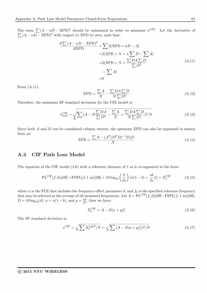
Appendix A: Path Loss Model Parameter Closed-Form Expressions 61
The term∑
(A− nD − XPD)2 should be minimized in order to minimize σCIX. Let the derivative of∑(A− nD − XPD)2 with respect to XPD be zero, such that:
∂∑
(A− nD − XPD)2
∂XPD=∑
2(XPD + nD −A)
=2(XPD ×N + n∑
D −∑
A)
=2(XPD ×N +
∑DA
∑D∑
D2
−∑
A)
=0
(A.11)
From (A.11):
XPD =
∑A
N−∑DA
∑D
N∑D2
(A.12)
Therefore, the minimum SF standard deviation for the CIX model is:
σCIXmin =
√∑(A−D
∑DA∑D2
−∑A
N+
∑DA
∑D
N∑D2
)2/N (A.13)
Since both A and D can be considered column vectors, the optimum XPD can also be expressed in matrixform as:
XPD =
∑A− (AT (DTD)−1D)D
N(A.14)
A.3 CIF Path Loss Model
The equation of the CIF model (4.6) with a reference distance of 1 m is re-organized in the form:
PLCIF(f, d)[dB] =FSPL(f, 1 m)[dB] + 10 log10
(d
d0
)(n(1 − b) +
nb
f0f) +XCIF
σ (A.15)
where n is the PLE that includes the frequency-effect parameter b, and f0 is the specified reference frequencythat may be selected as the average of all measured frequencies. Let A = PLCIF(f, d)[dB]−FSPL(f, 1 m)[dB],D = 10 log10(d), a = n(1 − b), and g = nb
f0, then we have:
XCIFσ = A−D(a+ gf) (A.16)
The SF standard deviation is:
σCIF =√∑
XCIFσ
2/N =√∑
(A−D(a+ gf))2/N (A.17)
c© 2015 NYU WIRELESS
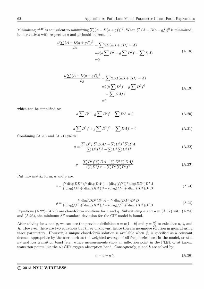
62 Appendix A: Path Loss Model Parameter Closed-Form Expressions
Minimizing σCIF is equivalent to minimizing∑
(A−D(a+ gf))2. When∑
(A−D(a+ gf))2 is minimized,its derivatives with respect to a and g should be zero, i.e.
∂∑
(A−D(a+ gf))2
∂a=∑
2D(aD + gDf −A)
=2(a∑
D2 + g∑
D2f −∑
DA)
=0
(A.18)
∂∑
(A−D(a+ gf))2
∂g=∑
2Df(aD + gDf −A)
=2(a∑
D2f + g∑
D2f2
−∑
DAf)
=0
(A.19)
which can be simplified to:
a∑
D2 + g∑
D2f −∑
DA = 0 (A.20)
a∑
D2f + g∑
D2f2 −∑
DAf = 0 (A.21)
Combining (A.20) and (A.21) yields:
a =
∑D2f
∑DAf −
∑D2f2
∑DA
(∑D2f2)2 −
∑D2∑D2f2
(A.22)
g =
∑D2f
∑DA−
∑D2∑DAf
(∑D2f)2 −
∑D2∑D2f2
(A.23)
Put into matrix form, a and g are:
a =fT diag(DDT )fT diag(DAT ) − (diag(ffT ))T diag(DDT )DTA
((diag(ffT ))T diag(DDT ))2 − (diag(ffT ))T diag(DDT )DTD(A.24)
g =fT diag(DDT )DTA− fT diag(DAT )DTD
((diag(ffT ))T diag(DDT ))2 − (diag(ffT ))T diag(DDT )DTD(A.25)
Equations (A.22)–(A.25) are closed-form solutions for a and g. Substituting a and g in (A.17) with (A.24)and (A.25), the minimum SF standard deviation for the CIF model is found.
After solving for a and g, we can use the previous definition a = n(1 − b) and g = nbf0
to calculate n, b, andf0. However, there are two equations but three unknowns, hence there is no unique solution in general usingthree parameters. However, a unique closed-form solution is available when f0 is specified as a constantdeemed appropriate by the user, such as the weighted average of all frequencies used in the model, or at anatural loss transition band (e.g., where measurements show an inflection point in the PLE), or at knowntransition points like the 60 GHz oxygen absorption band. Consequently, n and b are solved by:
n = a+ gf0 (A.26)
c© 2015 NYU WIRELESS
Appendix A: Path Loss Model Parameter Closed-Form Expressions 63
b =gf0
a+ gf0(A.27)
A.4 CIFX Path Loss Model
The CIFX path loss model (4.7) and also expressed as:
PLCIFX(f, d)[dB] =FSPL(f, 1 m)[dB] + 10 log10
(d
d0
)(a+ gf) + XPD +XCIFX
σ (A.28)
where XPD denotes the cross-polarization discrimination factor, n, b, and f0 have the same meanings as inthe CIF model (A.15). Note that the CIFX model (A.28) uses the same a and g as substituted in the CIFmodel (A.15), thus the a and g in (A.28) are also given by (A.24) and (A.25), respectively. The XPD issolved via the MMSE method that fits the measured cross-polarized path loss data with the smallest error(i.e., SF standard deviation).
Using the same notations as in the CIF model, the SF in the CIFX model can be expressed as
XCIFXσ = A− (a+ gf)D − XPD (A.29)
Hence the SF standard deviation is:
σCIFX =√∑
XCIFXσ
2/N
=√∑
(A− (a+ gf)D − XPD)2/N(A.30)
Thus the term∑
(A− (a+ gf)D − XPD)2 should be minimized in order to minimize σCIFX. With thederivative of
∑(A− (a+ gf)D − XPD)2 with respect to XPD set to zero, we have:
∂∑
(A− (a+ gf)D − XPD)2
∂XPD
=∑
2(XPD + (a+ gf)D −A)
=2(XPD ×N + a∑
D + g∑
Df −∑
A)
=0
(A.31)
From (A.11):
XPD =
∑A− a
∑D − g
∑Df
N(A.32)
Or equivalently
XPD =
∑A− a
∑D − gDT f
N(A.33)
Therefore, by plugging (A.24), (A.25) and (A.32) back into (A.30), the minimum SF standard deviation forthe CIFX model is found.
c© 2015 NYU WIRELESS
64 Appendix A: Path Loss Model Parameter Closed-Form Expressions
A.5 FI Path Loss Model
The FI path loss model (4.3) uses α as the floating intercept in dB (different from a FSPL reference), and βis the slope of the line (different from a PLE). Assuming B = PLABG(d)[dB], and D = 10 log10(d), the SFis given by:
XFIσ = B − α− βD (A.34)
and the SF standard deviation is:
σFI =√∑
XFIσ
2/N =√∑
(B − α− βD)2/N (A.35)
The term∑
(B − α− βD)2 is to be minimized, which means its partial derivatives with respect to α and βshould be zero, i.e.,
∂∑
(B − α− βD)2
∂α=∑
2(α+ βD −B)
=2(Nα+ β∑
D −∑
B)
=0
(A.36)
∂∑
(B − α− βD)2
∂β=∑
2D(α+ βD −B)
=2(α∑
D + β∑
D2 −∑
DB)
=0
(A.37)
(A.36) and (A.37) yield:
Nα+ β∑
D −∑
B = 0 (A.38)
α∑
D + β∑
D2 −∑
DB (A.39)
Combining (A.38) and (A.39) yields:
α =
∑D∑DB −
∑D2∑B
(∑D)2 −N
∑D2
(A.40)
β =
∑D∑B −N
∑DB
(∑D)2 −N
∑D2
(A.41)
The minimum SF standard deviation can be obtained by substituting α and β in (A.35) with (A.40)and (A.41), respectively. Alternatively, α and β in the FI model can be expressed in matrix form as
β = (D −D)T ((D −D)T (D −D))−1(B −B) (A.42)
α = B − βD (A.43)
c© 2015 NYU WIRELESS
Appendix A: Path Loss Model Parameter Closed-Form Expressions 65
where D and B denote the mean value of the elements in column vectors D and B, respectively. All themean values are calculated directly from the elements in the vector, i.e., if the elements are in dB scale thenthe mean is calculated directly in dB scale.
A.6 ABG Path Loss Model
The ABG model (4.4) has a 1 m reference distance and 1 GHz reference frequency) where α and γ arecoefficients showing the dependence of path loss on distance and frequency, respectively, β is the offset inpath loss, d is the 3D T-R separation distance in meters, and f is the carrier frequency in GHz. AssumingB = PLABG(f, d)[dB], D = 10 log10(d), and F = 10 log10(f) in (4.4), the SF is given by:
XABGσ = B − αD − β − γF (A.44)
and the SF standard deviation is:
σABG =√∑
XABGσ
2/N =√∑
(B − αD − β − γF )2/N (A.45)
Similar to minimizing Eqs. (A.2) and (A.17) the term∑
(B − αD − β − γF )2 is to be minimized, whichmeans its partial derivatives with respect to α, β, and γ should be zero, i.e.,
∂∑
(B − αD − β − γF )2
∂α=∑
2D(αD + β + γF −B)
=2(α∑
D2 + β∑
D
+ γ∑
DF −∑
DB)
=0
(A.46)
∂∑
(B − αD − β − γF )2
∂β=∑
2(αD + β + γF −B)
=2(α∑
D +Nβ + γ∑
F
−∑
B)
=0
(A.47)
∂∑
(B − αD − β − γF )2
∂γ=∑
2F (αD + β + γF −B)
=2(α∑
DF + β∑
F
+ γ∑
F 2 −∑
FB)
=0
(A.48)
from (A.46), (A.47), and (A.48) it is clear that
α∑
D2 + β∑
D + γ∑
DF −∑
DB = 0 (A.49)
c© 2015 NYU WIRELESS

66 Appendix A: Path Loss Model Parameter Closed-Form Expressions
α∑
D +Nβ + γ∑
F −∑
B = 0 (A.50)
α∑
DF + β∑
F + γ∑
F 2 −∑
FB = 0 (A.51)
Such that (A.49), (A.50), and (A.51) in matrix form is:∑D2∑D
∑DF∑
D N∑F∑
DF∑F
∑F 2
αβγ
=
∑DB∑B∑FB
(A.52)
Through calculation and simplification, the closed-form solutions for α, β, and γ are given by (A.55), (A.56),and (A.57), respectively. Equations (A.58), (A.59), and (A.60) show the solutions in matrix form. Finally, theminimum SF standard deviation for the ABG model can be obtained by plugging (A.55), (A.56), and (A.57)back into (A.45). Or a system of simultaneous equations allow for α, β, and γ to be found by:αβ
γ
=
∑D2∑D
∑DF∑
D N∑F∑
DF∑F
∑F 2
−1∑DB∑B∑FB
(A.53)
A.7 ABGX Path Loss Model
The ABGX model (4.5) is found in the exact same manner as the CIX and CIFX models. The α, β, and γvalues found for the co-polarized ABG model (4.4) are substituted into the right hand side of (4.4) for allmeasured distances d to form a vector of estimated path loss values, specified as ABGPL. Then using thecross-polarized path loss values in vector form A from measurements, the XPD factor for the ABGX modelis:
XPD =
∑A−ABGPL
N(A.54)
α =(∑D∑B −N
∑DB)((
∑F )2 −N
∑F 2) − (
∑D∑F −N
∑DF )(
∑F∑B −N
∑FB)
((∑D)2 −N
∑D2)((
∑F )2 −N
∑F 2) − (
∑D∑F −N
∑DF )2
(A.55)
β =(∑D∑FB −
∑B∑DF )(
∑F∑D2 −
∑D∑DF ) − (
∑B∑D2 −
∑D∑DB)(
∑D∑F 2 −
∑F∑DF )
((∑D)2 −N
∑D2)(
∑D∑F 2 −
∑F∑DF ) + (
∑D∑F −N
∑DF )(
∑F∑D2 −
∑D∑DF )
(A.56)
γ =(∑F∑B −N
∑FB)((
∑D)2 −N
∑D2) − (
∑D∑F −N
∑DF )(
∑D∑B −N
∑DB)
((∑F )2 −N
∑F 2)((
∑D)2 −N
∑D2) − (
∑D∑F −N
∑DF )2
(A.57)
α =(∑D∑B −NDTB)((
∑F )2 −NF TF ) − (
∑D∑F −NDTF )(
∑F∑B −NF TB)
((∑D)2 −NDTD)((
∑F )2 −NF TF ) − (
∑D∑F −NDTF )2
(A.58)
c© 2015 NYU WIRELESS
Appendix A: Path Loss Model Parameter Closed-Form Expressions 67
β =(FTB
∑D −DTF
∑B)(DTD
∑F −DTF
∑D) − (DTD
∑B −DTB
∑D)(FTF
∑D −DTF
∑F )
((∑D)2 −NDTD)(FTF
∑D −DTF
∑F ) + (
∑D∑F −NDTF )(DTD
∑F −DTF
∑D)
(A.59)
γ =(∑F∑B −NFTB)((
∑D)2 −NDTD) − (
∑D∑F −NDTF )(
∑D∑B −NDTB)
((∑F )2 −NFTF )((
∑D)2 −NDTD) − (
∑D∑F −NDTF )2
(A.60)
c© 2015 NYU WIRELESS

This page is intentionally left blank.
Appendix B
Omnidirectional Path Loss Values
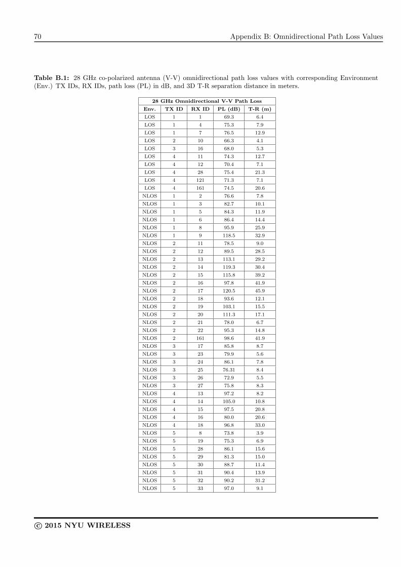
70 Appendix B: Omnidirectional Path Loss Values
Table B.1: 28 GHz co-polarized antenna (V-V) omnidirectional path loss values with corresponding Environment(Env.) TX IDs, RX IDs, path loss (PL) in dB, and 3D T-R separation distance in meters.
28 GHz Omnidirectional V-V Path Loss
Env. TX ID RX ID PL (dB) T-R (m)
LOS 1 1 69.3 6.4
LOS 1 4 75.3 7.9
LOS 1 7 76.5 12.9
LOS 2 10 66.3 4.1
LOS 3 16 68.0 5.3
LOS 4 11 74.3 12.7
LOS 4 12 70.4 7.1
LOS 4 28 75.4 21.3
LOS 4 121 71.3 7.1
LOS 4 161 74.5 20.6
NLOS 1 2 76.6 7.8
NLOS 1 3 82.7 10.1
NLOS 1 5 84.3 11.9
NLOS 1 6 86.4 14.4
NLOS 1 8 95.9 25.9
NLOS 1 9 118.5 32.9
NLOS 2 11 78.5 9.0
NLOS 2 12 89.5 28.5
NLOS 2 13 113.1 29.2
NLOS 2 14 119.3 30.4
NLOS 2 15 115.8 39.2
NLOS 2 16 97.8 41.9
NLOS 2 17 120.5 45.9
NLOS 2 18 93.6 12.1
NLOS 2 19 103.1 15.5
NLOS 2 20 111.3 17.1
NLOS 2 21 78.0 6.7
NLOS 2 22 95.3 14.8
NLOS 2 161 98.6 41.9
NLOS 3 17 85.8 8.7
NLOS 3 23 79.9 5.6
NLOS 3 24 86.1 7.8
NLOS 3 25 76.31 8.4
NLOS 3 26 72.9 5.5
NLOS 3 27 75.8 8.3
NLOS 4 13 97.2 8.2
NLOS 4 14 105.0 10.8
NLOS 4 15 97.5 20.8
NLOS 4 16 80.0 20.6
NLOS 4 18 96.8 33.0
NLOS 5 8 73.8 3.9
NLOS 5 19 75.3 6.9
NLOS 5 28 86.1 15.6
NLOS 5 29 81.3 15.0
NLOS 5 30 88.7 11.4
NLOS 5 31 90.4 13.9
NLOS 5 32 90.2 31.2
NLOS 5 33 97.0 9.1
c© 2015 NYU WIRELESS

Appendix B: Omnidirectional Path Loss Values 71
Table B.2: 28 GHz cross-polarized antenna (V-H) omnidirectional path loss values with corresponding Environment(Env.) TX IDs, RX IDs, path loss (PL) in dB, and 3D T-R separation distance in meters.
28 GHz Omnidirectional V-H Path Loss
Env. TX ID RX ID PL (dB) T-R (m)
LOS 1 1 84.1 6.4
LOS 1 4 87.7 7.9
LOS 1 7 89.7 12.9
LOS 2 10 78.6 4.1
LOS 3 16 83.4 5.3
LOS 4 11 88.2 12.7
LOS 4 12 85.1 7.1
LOS 4 28 90.2 21.3
LOS 4 121 85.0 7.1
LOS 4 161 89.8 20.6
NLOS 1 2 88.2 7.8
NLOS 1 3 91.3 10.1
NLOS 1 5 94.7 11.9
NLOS 1 6 100.1 14.4
NLOS 1 8 115.3 25.9
NLOS 2 11 88.5 9.0
NLOS 2 12 108.8 28.5
NLOS 2 13 141.6 29.2
NLOS 2 14 139.6 30.4
NLOS 2 16 113.4 41.9
NLOS 2 18 98.9 12.1
NLOS 2 19 113.7 15.5
NLOS 2 20 120.4 17.1
NLOS 2 21 83.7 6.7
NLOS 2 22 101.6 14.8
NLOS 2 161 110.5 41.9
NLOS 3 17 97.2 8.7
NLOS 3 23 92.7 5.6
NLOS 3 24 95.8 7.8
NLOS 3 25 88.9 8.4
NLOS 3 26 86.7 5.5
NLOS 3 27 89.3 8.3
NLOS 4 13 104.6 8.2
NLOS 4 14 112.8 10.8
NLOS 4 15 108.4 20.8
NLOS 4 16 93.7 20.6
NLOS 4 18 109.4 33.0
NLOS 5 8 89.3 3.9
NLOS 5 19 91.5 6.9
NLOS 5 28 98.4 15.6
NLOS 5 29 93.7 15.0
NLOS 5 30 96.1 11.4
NLOS 5 31 100.2 13.9
NLOS 5 32 104.8 31.2
NLOS 5 33 104.6 9.1
c© 2015 NYU WIRELESS
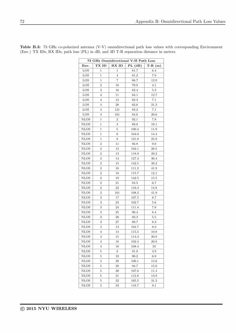
72 Appendix B: Omnidirectional Path Loss Values
Table B.3: 73 GHz co-polarized antenna (V-V) omnidirectional path loss values with corresponding Environment(Env.) TX IDs, RX IDs, path loss (PL) in dB, and 3D T-R separation distance in meters.
73 GHz Omnidirectional V-H Path Loss
Env. TX ID RX ID PL (dB) T-R (m)
LOS 1 1 81.7 6.4
LOS 1 4 81.2 7.9
LOS 1 7 86.7 12.9
LOS 2 10 79.9 4.1
LOS 3 16 82.4 5.3
LOS 4 11 84.1 12.7
LOS 4 12 82.3 7.1
LOS 4 28 82.6 21.3
LOS 4 121 83.2 7.1
LOS 4 161 84.6 20.6
NLOS 1 2 92.1 7.8
NLOS 1 3 89.8 10.1
NLOS 1 5 100.4 11.9
NLOS 1 6 104.0 14.4
NLOS 1 8 121.8 25.9
NLOS 2 11 92.8 9.0
NLOS 2 12 102.1 28.5
NLOS 2 13 118.9 29.2
NLOS 2 14 127.4 30.4
NLOS 2 15 142.5 39.2
NLOS 2 16 111.2 41.9
NLOS 2 18 115.7 12.1
NLOS 2 19 142.5 15.5
NLOS 2 21 94.5 6.7
NLOS 2 22 116.3 14.8
NLOS 2 161 108.2 41.9
NLOS 3 17 107.5 8.7
NLOS 3 23 102.7 5.6
NLOS 3 24 111.4 7.8
NLOS 3 25 90.4 8.4
NLOS 3 26 93.3 5.5
NLOS 3 27 89.7 8.3
NLOS 4 13 104.7 8.2
NLOS 4 14 115.5 10.8
NLOS 4 15 114.2 20.8
NLOS 4 16 102.4 20.6
NLOS 4 18 108.4 33
NLOS 5 8 91.0 3.9
NLOS 5 19 90.2 6.9
NLOS 5 28 100.1 15.6
NLOS 5 29 94.7 15.0
NLOS 5 30 107.6 11.4
NLOS 5 31 112.8 13.9
NLOS 5 32 105.5 31.2
NLOS 5 33 118.7 9.1
c© 2015 NYU WIRELESS
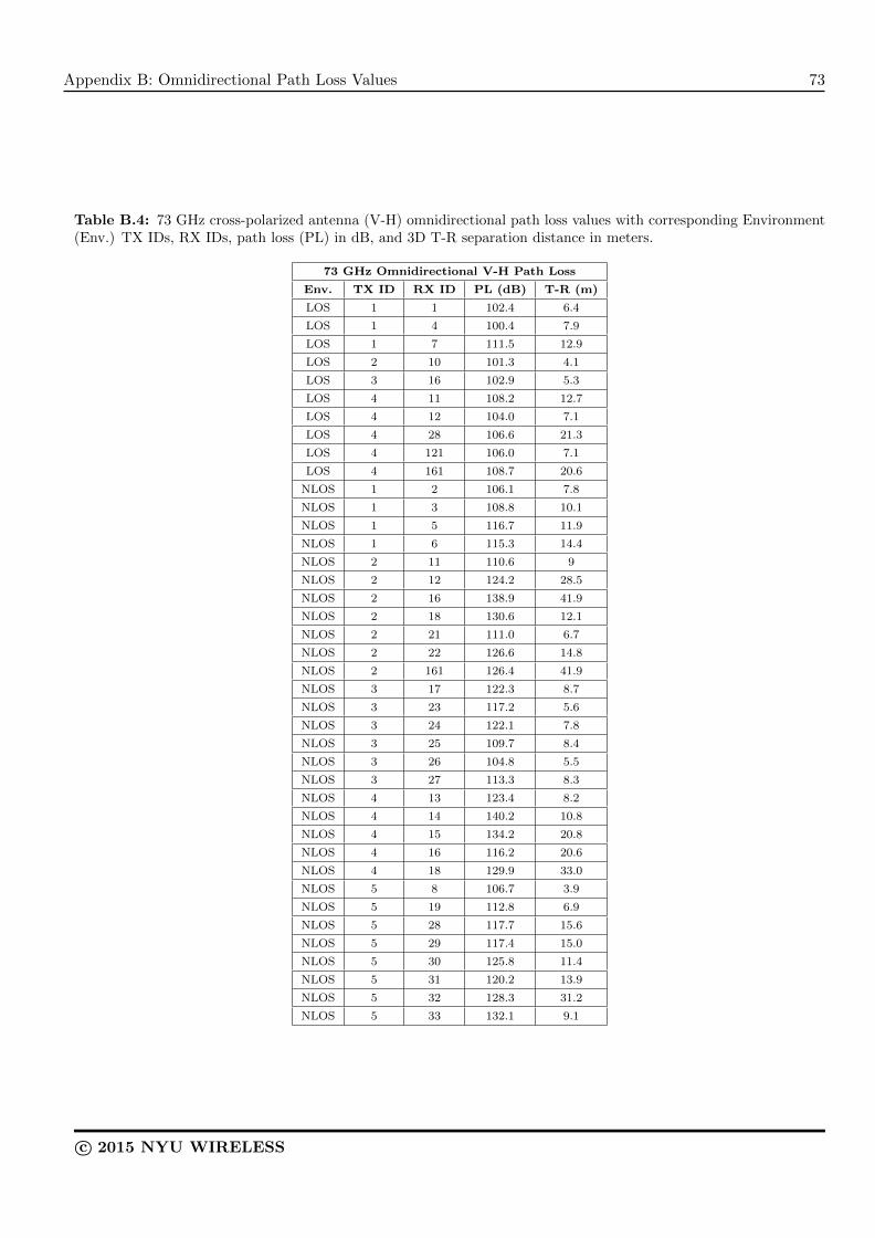
Appendix B: Omnidirectional Path Loss Values 73
Table B.4: 73 GHz cross-polarized antenna (V-H) omnidirectional path loss values with corresponding Environment(Env.) TX IDs, RX IDs, path loss (PL) in dB, and 3D T-R separation distance in meters.
73 GHz Omnidirectional V-H Path Loss
Env. TX ID RX ID PL (dB) T-R (m)
LOS 1 1 102.4 6.4
LOS 1 4 100.4 7.9
LOS 1 7 111.5 12.9
LOS 2 10 101.3 4.1
LOS 3 16 102.9 5.3
LOS 4 11 108.2 12.7
LOS 4 12 104.0 7.1
LOS 4 28 106.6 21.3
LOS 4 121 106.0 7.1
LOS 4 161 108.7 20.6
NLOS 1 2 106.1 7.8
NLOS 1 3 108.8 10.1
NLOS 1 5 116.7 11.9
NLOS 1 6 115.3 14.4
NLOS 2 11 110.6 9
NLOS 2 12 124.2 28.5
NLOS 2 16 138.9 41.9
NLOS 2 18 130.6 12.1
NLOS 2 21 111.0 6.7
NLOS 2 22 126.6 14.8
NLOS 2 161 126.4 41.9
NLOS 3 17 122.3 8.7
NLOS 3 23 117.2 5.6
NLOS 3 24 122.1 7.8
NLOS 3 25 109.7 8.4
NLOS 3 26 104.8 5.5
NLOS 3 27 113.3 8.3
NLOS 4 13 123.4 8.2
NLOS 4 14 140.2 10.8
NLOS 4 15 134.2 20.8
NLOS 4 16 116.2 20.6
NLOS 4 18 129.9 33.0
NLOS 5 8 106.7 3.9
NLOS 5 19 112.8 6.9
NLOS 5 28 117.7 15.6
NLOS 5 29 117.4 15.0
NLOS 5 30 125.8 11.4
NLOS 5 31 120.2 13.9
NLOS 5 32 128.3 31.2
NLOS 5 33 132.1 9.1
c© 2015 NYU WIRELESS

This page is intentionally left blank.
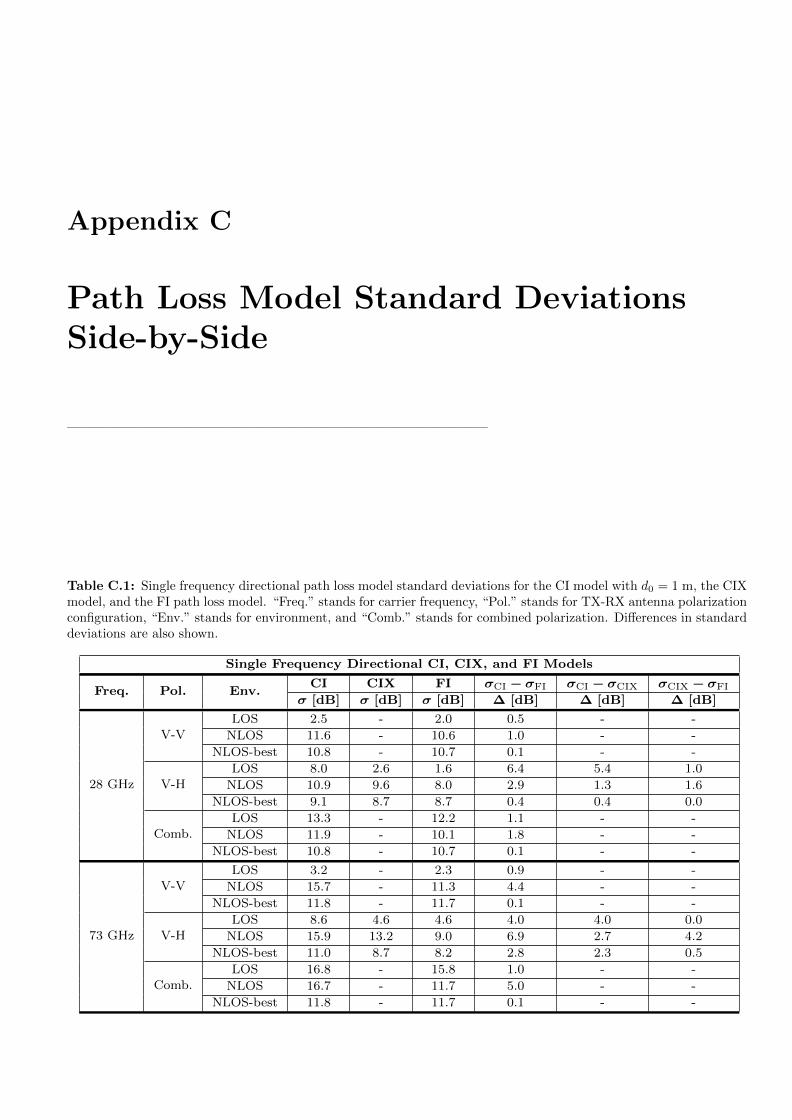
Appendix C
Path Loss Model Standard DeviationsSide-by-Side
—————————————————————————————
Table C.1: Single frequency directional path loss model standard deviations for the CI model with d0 = 1 m, the CIXmodel, and the FI path loss model. “Freq.” stands for carrier frequency, “Pol.” stands for TX-RX antenna polarizationconfiguration, “Env.” stands for environment, and “Comb.” stands for combined polarization. Differences in standarddeviations are also shown.
Single Frequency Directional CI, CIX, and FI Models
Freq. Pol. Env.CI CIX FI σCI − σFI σCI − σCIX σCIX − σFI
σ [dB] σ [dB] σ [dB] ∆ [dB] ∆ [dB] ∆ [dB]
28 GHz
V-VLOS 2.5 - 2.0 0.5 - -
NLOS 11.6 - 10.6 1.0 - -
NLOS-best 10.8 - 10.7 0.1 - -
V-HLOS 8.0 2.6 1.6 6.4 5.4 1.0
NLOS 10.9 9.6 8.0 2.9 1.3 1.6
NLOS-best 9.1 8.7 8.7 0.4 0.4 0.0
Comb.LOS 13.3 - 12.2 1.1 - -
NLOS 11.9 - 10.1 1.8 - -
NLOS-best 10.8 - 10.7 0.1 - -
73 GHz
V-VLOS 3.2 - 2.3 0.9 - -
NLOS 15.7 - 11.3 4.4 - -
NLOS-best 11.8 - 11.7 0.1 - -
V-HLOS 8.6 4.6 4.6 4.0 4.0 0.0
NLOS 15.9 13.2 9.0 6.9 2.7 4.2
NLOS-best 11.0 8.7 8.2 2.8 2.3 0.5
Comb.LOS 16.8 - 15.8 1.0 - -
NLOS 16.7 - 11.7 5.0 - -
NLOS-best 11.8 - 11.7 0.1 - -

76 Appendix C: Path Loss Model Standard Deviations Side-by-Side
Table C.2: Multi-frequency directional path loss model standard deviations for the CI, CIX, CIF, CIFX, ABG, andABGX large-scale path loss models. “Pol.” stands for TX-RX antenna polarization configuration, “Env.” stands forenvironment, and “Comb.” stands for combined polarization. Differences in standard deviations are also shown.
Multi-Frequency Directional CI(X), CIF(X), and ABG(X) Models
Pol. Env.CI CIF ABG σCI − σCIF σCI − σABG σCIF − σABG
σ [dB] σ [dB] σ [dB] ∆ [dB] ∆ [dB] ∆ [dB]
V-VLOS 2.9 2.9 2.1 0.0 0.8 0.8
NLOS 14.6 13.9 11.1 0.7 3.5 2.8
NLOS-best 11.5 11.3 11.2 0.2 0.3 0.1
Pol. Env.CIX CIFX ABGX σCIX − σCIFX σCIX − σABGX σCIFX − σABGX
σ [dB] σ [dB] σ [dB] ∆ [dB] ∆ [dB] ∆ [dB]
V-HLOS 4.7 5.0 4.9 -0.3 -0.2 0.1
NLOS 13.3 11.8 8.7 1.5 4.6 3.1
NLOS-best 9.6 9.0 8.8 0.6 0.8 0.2
Pol. Env.CI CIF ABG σCI − σCIF σCI − σABG σCIF − σABG
σ [dB] σ [dB] σ [dB] ∆ [dB] ∆ [dB] ∆ [dB]
Comb.LOS 15.2 15.2 14.2 0.0 1.0 1.0
NLOS 15.5 14.5 11.0 1.0 4.5 3.5
NLOS-best 11.5 11.3 11.2 0.2 0.3 0.1
Table C.3: Single frequency omnidirectional path loss model standard deviations for the CI model with d0 = 1 m,the CIX model, and the FI path loss model. “Freq.” stands for carrier frequency, “Pol.” stands for TX-RX antennapolarization configuration, “Env.” stands for environment, and “Comb.” stands for combined polarization. Differencesin standard deviations are also shown.
Single Frequency Omnidirectional CI, CIX, and FI Models
Freq. Pol. Env.CI CIX FI σCI − σFI σCI − σCIX σCIX − σFI
σ [dB] σ [dB] σ [dB] ∆ [dB] ∆ [dB] ∆ [dB]
28 GHz
V-VLOS 1.8 - 1.8 0.0 - -
NLOS 9.6 - 9.3 0.3 - -
V-HLOS 3.0 1.5 1.4 1.6 1.5 0.1
NLOS 9.4 9.7 9.4 0.0 -0.3 0.3
Comb.LOS 7.3 - 7.2 0.1 - -
NLOS 10.9 - 10.9 0.0 - -
73 GHz
V-VLOS 2.4 - 1.4 1.0 - -
NLOS 11.3 - 11.2 0.1 - -
V-HLOS 6.3 2.4 2.3 4.0 3.9 0.1
NLOS 9.7 8.0 7.5 2.2 1.7 0.5
Comb.LOS 12.0 - 11.3 0.7 - -
NLOS 12.9 - 12.1 0.8 - -
c© 2015 NYU WIRELESS

Appendix C: Path Loss Model Standard Deviations Side-by-Side 77
Table C.4: Multi-frequency omnidirectional path loss model standard deviations for the CI, CIX, CIF, CIFX, ABG,and ABGX large-scale path loss models. “Pol.” stands for TX-RX antenna polarization configuration, “Env.” standsfor environment, and “Comb.” stands for combined polarization. Differences in standard deviations are also shown.
Multi-Frequency Omnidirectional CI(X), CIF(X), and ABG(X) Models
Pol. Env.CI CIF ABG σCI − σCIF σCI − σABG σCIF − σABG
σ [dB] σ [dB] σ [dB] ∆ [dB] ∆ [dB] ∆ [dB]
V-VLOS 2.3 2.1 1.8 0.2 0.5 0.3
NLOS 10.9 10.4 10.3 0.5 0.6 0.1
Pol. Env.CIX CIFX ABGX σCIX − σCIFX σCIX − σABGX σCIFX − σABGX
σ [dB] σ [dB] σ [dB] ∆ [dB] ∆ [dB] ∆ [dB]
V-HLOS 5.7 4.8 4.7 0.9 1.0 0.1
NLOS 10.4 9.3 9.0 1.1 1.4 0.3
Pol. Env.CI CIF ABG σCI − σCIF σCI − σABG σCIF − σABG
σ [dB] σ [dB] σ [dB] ∆ [dB] ∆ [dB] ∆ [dB]
Comb.LOS 10.4 9.9 9.5 0.5 0.9 0.4
NLOS 12.5 11.9 11.6 0.6 0.9 0.3
c© 2015 NYU WIRELESS

This page is intentionally left blank.

Bibliography
[1] Z. Pi and F. Khan, “An introduction to millimeter-wave mobile broadband systems,” IEEE Commu-nications Magazine, vol. 49, no. 6, pp. 101–107, June 2011.
[2] L. Yinzhou, J. Yang, and N. Ansari, “Cellular smartphone traffic and user behavior analysis,” in 2014IEEE International Conference on Communications (ICC), June 2014, pp. 1326–1331.
[3] T. S. Rappaport, “Keynote Speech: Millimeter Wave Wireless Communications - The Renaissance ofComputing and Communications,” in 2014 IEEE International Conference on Communications (ICC),Sydney, Australia, June 2014. [Online]. Available: http://icc2014.ieee-icc.org/speakers 28 4101586138.pdf
[4] F. Aldhaban, “Exploring the adoption of smartphone technology: Literature review,” in Proceedings ofPICMET ’12: Technology Management for Emerging Technologies (PICMET), July 2012, pp. 2758–2770.
[5] Gartner, “Gartner says by 2018, more than 50 percent of users will use a tablet or smartphone first forall online activities,” Dec. 2014. [Online]. Available: http://www.gartner.com/newsroom/id/2939217
[6] T. S. Rappaport, S. Sun, R. Mayzus, H. Zhao, Y. Azar, K. Wang, G. N. Wong, J. K. Schulz, M. K.Samimi, and F. Gutierrez, Jr., “Millimeter Wave Mobile Communications for 5G Cellular: It WillWork!” IEEE Access, vol. 1, pp. 335–349, 2013.
[7] T. S. Rappaport, R. W. Heath, Jr., R. C. Daniels, and J. N. Murdock, Millimeter Wave WirelessCommunications. Pearson/Prentice Hall, 2015.
[8] CISCO, “20 Myths of Wi-Fi Interference: Dispel Myths to Gain High Performing and ReliableWireless,” 2007. [Online]. Available: http://www.cisco.com/c/en/us/products/collateral/wireless/spectrum-expert-wi-fi/prod white paper0900aecd807395a9.pdf
[9] Z. Hays, G. Richter, S. Berger, C. Baylis, and R. J. Marks, “Alleviating airport WiFi congestion:An comparison of 2.4 GHz and 5 GHz WiFi usage and capabilities,” in 2014 Texas Symposium onWireless and Microwave Circuits and Systems (WMCS), Apr. 2014, pp. 1–4.
[10] C. Na, J. K. Chen, and T. S. Rappaport, “Hotspot traffic statistics and throughput models for severalapplications,” in 2004 Proceedings of the Global Telecommunications Conference (GLOBECOM), 2004,pp. 3257–3263.
[11] ——, “Measured traffic statistics and throughput of IEEE 802.11b public WLAN hotspots with threedifferent applications,” IEEE Transactions on Wireless Communications, vol. 5, no. 11, pp. 3296–3305,2006.
[12] C. Sergiou, P. Antoniou, and V. Vassiliou, “A comprehensive survey of congestion control protocolsin wireless sensor networks,” IEEE Communications Surveys Tutorials, vol. 16, no. 4, pp. 1839–1859,2014.
79
80 Bibliography
[13] H. Xu, V. Kukshya, and T. S. Rappaport, “Spatial and temporal characteristics of 60-GHz indoorchannels,” IEEE Journal on Selected Areas in Communications, vol. 20, no. 3, pp. 620–630, Apr.2002.
[14] A. Maltsev, R. Maslennikov, A. Sevastyanov, A. Khoryaev, and A. Lomayev, “Experimental investi-gations of 60 GHz WLAN systems in office environment,” IEEE Journal on Selected Areas in Com-munications, vol. 27, no. 8, pp. 1488–1499, Oct. 2009.
[15] X. Ge, H. Cheng, M. Guizani, and T. Han, “5G wireless backhaul networks: challenges and researchadvances,” IEEE Network, vol. 28, no. 6, pp. 6–11, Nov. 2014.
[16] S. E. Alexander, “Characterising buildings for propagation at 900 MHz,” Electronics Letters, vol. 19,no. 20, pp. 860–861, Sept. 1983.
[17] D. Akerberg, “Properties of a TDMA pico cellular office communication system,” in IEEE 39th Ve-hicular Technology Conference, vol. 1, May 1989, pp. 186–191.
[18] A. A. M. Saleh and R. A. Valenzuela, “A statistical model for indoor multipath propagation,” IEEEJournal on Selected Areas in Communications, vol. 5, no. 2, pp. 128–137, Feb. 1987.
[19] R. J. C. Bultitude, “Measurement, characterization and modeling of indoor 800/900 MHz radio chan-nels for digital communications,” IEEE Communications Magazine, vol. 25, no. 6, pp. 5–12, June1987.
[20] A. J. Motley and J. Keenan, “Personal communication radio coverage in buildings at 900 MHz and1700 MHz,” Electronics Letters, vol. 24, no. 12, pp. 763–764, Jun. 1988.
[21] T. S. Rappaport, “Characterization of UHF multipath radio channels in factory buildings,” IEEETransactions on Antennas and Propagation, vol. 37, no. 8, pp. 1058–1069, Aug. 1989.
[22] T. S. Rappaport and D. A. Hawbaker, “Effects of circular and linear polarized antennas on wide-band propagation parameters in indoor radio channels,” in Global Telecommunications Conference,1991. GLOBECOM ’91. Countdown to the New Millennium. Featuring a Mini-Theme on: PersonalCommunications Services, vol. 2, Dec. 1991, pp. 1287–1291.
[23] A. F. Molisch, L. J. Greenstein, and M. Shafi, “Propagation issues for cognitive radio,” Proceedings ofthe IEEE, vol. 97, no. 5, pp. 787–804, May 2009.
[24] C. Ho, T. S. Rappaport, and M. P. Koushik, “Antenna effects on indoor obstructed wireless channelsand a deterministic image-based wide-band propagation model for in-building personal communicationsystems,” International Journal of Wireless Information Networks, vol. 1, no. 1, pp. 61–76, Jan. 1994.
[25] J. B. Andersen, T. S. Rappaport, and S. Yoshida, “Propagation measurements and models for wirelesscommunications channels,” IEEE Communications Magazine, vol. 33, no. 1, pp. 42–49, Jan. 1995.
[26] T. S. Rappaport and S. Sandhu, “Radio-wave propagation for emerging wireless personal-communication systems,” IEEE Antennas and Propagation Magazine, vol. 36, no. 5, pp. 14–24, Oct.1994.
[27] A. Alvarez, G. Valera, M. Lobeira, R. P. Torres, and J. L. Garcia, “Ultra wideband channel model forindoor environments,” Journal of Communications and Networks, vol. 5, no. 4, pp. 309–318, 2003.
[28] S. S. Ghassemzadeh, R. Jana, C. W. Rice, W. Turin, and V. Tarokh, “Measurement and modelingof an ultra-wide bandwidth indoor channel,” IEEE Transactions on Communications, vol. 52, no. 10,pp. 1786–1796, Oct. 2004.

Bibliography 81
[29] G. D. Durgin, T. S. Rappaport, and H. Xu, “Partition-based path loss analysis for in-home andresidential areas at 5.85 GHz,” in IEEE Global Telecommunications Conference. GLOBECOM 1998:The Bridge to Global Integration, vol. 2, Nov. 1998, pp. 904–909.
[30] ——, “Radio path loss and penetration loss measurements in and around homes and trees at 5.85GHz,” in IEEE Antennas and Propagation Society International Symposium, vol. 2, June 1998, pp.618–621.
[31] ——, “5.85-GHz radio path loss and penetration loss measurements in and around homes and trees,”IEEE Communications Letters, vol. 2, no. 3, pp. 70–72, Mar. 1998.
[32] ——, “Measurements and models for radio path loss and penetration loss in and around homes andtrees at 5.85 GHz,” IEEE Transactions on Communications, vol. 46, no. 11, pp. 1484–1496, Nov. 1998.
[33] G. D. Durgin, V. Kukshya, and T. S. Rappaport, “Wideband measurements of angle and delay dis-persion for outdoor and indoor peer-to-peer radio channels at 1920 MHz,” IEEE Transactions onAntennas and Propagation, vol. 51, no. 5, pp. 936–944, May 2003.
[34] ——, “Joint angle and delay spread statistics for 1920 MHz peer-to-peer wireless channels,” in IEEEAntennas and Propagation Society International Symposium, vol. 2, July 2001, pp. 182–185.
[35] N. Patwari, G. D. Durgin, T. S. Rappaport, and R. J. Boyle, “Peer-to-peer low antenna outdoor radiowave propagation at 1.8 GHz,” in IEEE 49th Vehicular Technology Conference, vol. 1, Jul. 1999, pp.371–375.
[36] J. W. McKown and R. L. Hamilton, Jr., “Ray tracing as a design tool for radio networks,” IEEENetwork, vol. 5, no. 6, pp. 27–30, Nov. 1991.
[37] G. E. Athanasiadou, A. R. Nix, and J. P. McGeehan, “A ray tracing algorithm for microcellularwideband propagation modelling,” in IEEE 45th Vehicular Technology Conference, vol. 1, Jul. 1995,pp. 261–265.
[38] K. R. Schaubach, N. J. Davis, and T. S. Rappaport, “A ray tracing method for predicting path lossand delay spread in microcellular environments,” in IEEE 42nd Vehicular Technology Conference, May1992, pp. 932–935.
[39] S. Y. Seidel and T. S. Rappaport, “A ray tracing technique to predict path loss and delay spread insidebuildings,” in IEEE Global Telecommunications Conference, 1992, vol. 2, Dec. 1992, pp. 649–653.
[40] ——, “Site-specific propagation prediction for wireless in-building personal communication systemdesign,” IEEE Transactions on Vehicular Technology, vol. 43, no. 4, pp. 879–891, Nov. 1994.
[41] S. Y. Seidel, K. R. Schaubach, T. T. Tran, and T. S. Rappaport, “Research in site-specific propagationmodeling for pcs system design,” in 43rd IEEE Vehicular Technology Conference, May 1993, pp. 261–264.
[42] R. R. Skidmore, T. S. Rappaport, and A. L. Abbott, “Interactive coverage region and system designsimulation for wireless communication systems in multifloored indoor environments: SMT plus,” in5th IEEE International Conference on Universal Personal Communications, vol. 2, Sept. 1996, pp.646–650.
[43] S. Y. Seidel and T. S. Rappaport, “Path loss prediction in multifloored buildings at 914 MHz,” Elec-tronics Letters, vol. 40, no. 2, pp. 207–217, Feb 1992.
[44] G. D. Durgin, N. Patwari, and T. S. Rappaport, “Improved 3D ray launching method for wirelesspropagation prediction,” Electronics Letters, vol. 33, no. 16, pp. 1412–1413, July 1997.
82 Bibliography
[45] T. S. Rappaport et al., “Statistical channel impulse response models for factory and open plan buildingradio communication system design,” IEEE Transactions on Communications, vol. 39, no. 5, pp. 794–807, May 1991.
[46] T. S. Rappaport, W. Huang, and M. J. Feuerstein, “Performance of decision feedback equalizers insimulated urban and indoor radio channels,” in IEICE TRANSACTIONS on Communications, vol.E76-B, no. 2, Feb. 1993, pp. 78–79.
[47] T. S. Rappaport et al., “900-MHz multipath propagation measurements for US digital cellular ra-diotelephone,” IEEE Transactions on Vehicular Technology, vol. 39, no. 2, pp. 132–139, May 1990.
[48] S. Y. Seidel et al., “Path loss, scattering and multipath delay statistics in four European cities for digitalcellular and microcellular radiotelephone,” IEEE Transactions on Vehicular Technology, vol. 40, no. 4,pp. 721–730, Nov. 1991.
[49] T. S. Rappaport, Wireless Communications: Principles and Practice, 2nd ed. Upper Saddle River,NJ: Prentice Hall, 2002.
[50] J. E. Nuckols, “Implementation of geometrically based single-bounce models for simulation of angle-of-arrival of multipath delay components in the wireless channel simulation tools, SMRCIM and SIRCIM,”Virginia Tech Library, Master of Science, 1999.
[51] E. Perahia, C. Cordeiro, M. Park, and L. L. Yang, “IEEE 802.11ad: Defining the next generationmulti-Gbps Wi-Fi,” in 7th IEEE Consumer Communications and Networking Conference (CCNC),Jan. 2010, pp. 1–5.
[52] N. Guo, R. C. Qiu, S. Mo, and K. Takahashi, “60-GHz millimeter-wave radio: Principle, technology,and new results,” EURASIP Journal on Wireless Communications and Networking, vol. 2007, no. 1,pp. 48–48, 2007.
[53] R. C. Daniels, J. N. Murdock, T. S. Rappaport, and R. W. Heath, “60 GHz wireless: Up close andpersonal,” IEEE Microwave Magazine, vol. 11, pp. 44–55, Dec. 2010.
[54] S. K. Yong and C. C. Chong, “An overview of multigigabit wireless through millimeter wave technology:potentials and technical challenges,” EURASIP Journal on Wireless Communications and Networking,vol. 2007, no. 1, pp. 50–50, 2007.
[55] C. H. Doan, S. Emami, D. A. Sobel, A. M. Niknejad, and R. W. Brodersen, “Design considerationsfor 60 GHz CMOS radios,” IEEE Communications Magazine, vol. 42, no. 12, pp. 132–140, Dec. 2004.
[56] S. K. Reynolds, B. A. Floyd, U. R. Pfeiffer, T. Beukema, J. Grzyb, C. Haymes, B. Gaucher, andM. Soyuer, “A silicon 60-GHz receiver and transmitter chipset for broadband communications,” IEEEJournal of Solid-State Circuits, vol. 41, no. 12, pp. 2820–2831, Dec. 2006.
[57] F. Gutierrez, K. Parrish, and T. S. Rappaport, “On-chip integrated antenna structures in CMOS for60 GHz WPAN systems,” in IEEE Global Telecommunications Conference, 2009. GLOBECOM 2009,Nov 2009, pp. 1–7.
[58] M. Chelouche and A. Plattner, “Mobile broadband system (MBS): trends and impact on 60 GHz bandMMIC development,” Electronics Communication Engineering Journal, vol. 5, no. 3, pp. 187–197,June 1993.
[59] P. Smulders, “Exploiting the 60 GHz band for local wireless multimedia access: prospects and futuredirections,” IEEE Communications Magazine, vol. 40, no. 1, pp. 140–147, Jan. 2002.

Bibliography 83
[60] Y. Shoji, K. Hamaguchi, and H. Ogawa, “Millimeter-wave remote self-heterodyne system for extremelystable and low-cost broad-band signal transmission,” IEEE Transactions on Microwave Theory andTechniques, vol. 50, no. 6, pp. 1458–1468, June 2002.
[61] D. Cabric, M. S. Chen, D. A. Sobel, S. Wang, J. Yang, and R. W. Brodersen, “Novel radio architecturesfor uwb, 60 GHz, and cognitive wireless systems,” EURASIP Journal on Wireless Communicationsand Networking, no. 2, pp. 22–22, 2006.
[62] Y. Takimoto and T. Ihara, “Research activities on millimeter wave indoor communication systems injapan,” in IEEE MTT-S International Microwave Symposium Digest, Jun. 1993, pp. 673–676 vol.2.
[63] T. Ihara, T. Manabe, M. Fujita, T. Matsui, and Y. Sugimoto, “Research activities on millimeter-waveindoor wireless communication systems at CRL,” in 1995 Fourth IEEE International Conference onUniversal Personal Communications, Nov. 1995, pp. 197–200.
[64] P. Shrivastava and T. R. Rao, “Performance investigations with antipodal linear tapered slot antennaon 60 GHz radio link in a narrow hallway environment,” Progress In Electromagnetics Research C,vol. 58, pp. 69–77, 2015.
[65] A. Kumar and T. R. Rao, “Analysis of planning and deployment issues for short range gigabit radio’sat 60 GHz,” in International Conference on Communications and Signal Processing (ICCSP), April2013, pp. 24–28.
[66] S. Ramesh and T. R. Rao, “Indoor radio link characterization studies for millimeter wave wireless com-munications utilizing dielectric loaded exponentially tapered slot antenna,” Journal of ElectromagneticWaves and Applications, vol. 29, no. 4, pp. 551–564, Feb. 2015.
[67] P. F. M. Smulders and A. G. Wagemans, “Wide-band measurements of mm-wave indoor radio chan-nels,” in Third IEEE International Symposium on Personal, Indoor and Mobile Radio Communications(PIMRC), Oct. 1992, pp. 329–333.
[68] ——, “Wideband indoor radio propagation measurements at 58 GHz,” Electronics Letters, vol. 28,no. 13, pp. 1270–1272, June 1992.
[69] ——, “Frequency-domain measurement of the millimeter wave indoor radio channel,” IEEE Transac-tions on Instrumentation and Measurement, vol. 44, no. 6, pp. 1017–1022, Dec. 1995.
[70] H. Xu, V. Kukshya, and T. S. Rappaport, “Spatial and temporal characterization of 60 GHz indoorchannels,” in 52nd IEEE Vehicular Technology Conference (IEEE-VTS Fall VTC 2000), vol. 1, Sept.2000, pp. 6–13.
[71] M. Bensebti, J. P. McGeehan, and M. A. Beach, “Indoor multipath radio propagation measurementsand characterisation at 60 GHz,” in 21st European Microwave Conference, vol. 2, Sept. 1991, pp.1217–1222.
[72] T. Zwick, T. J. Beukema, and H. Nam, “Wideband channel sounder with measurements and modelfor the 60 GHz indoor radio channel,” IEEE Transactions on Vehicular Technology, vol. 54, no. 4, pp.1266–1277, July 2005.
[73] S. Geng, J. Kivinen, X. Zhao, and P. Vainikainen, “Millimeter-wave propagation channel characteriza-tion for short-range wireless communications,” IEEE Transactions on Vehicular Technology, vol. 58,no. 1, pp. 3–13, Jan. 2009.
[74] S. Geng, J. Kivinen, and P. Vainikainen, “Propagation characterization of wideband indoor radiochannels at 60 GHz,” in IEEE International Symposium on Microwave, Antenna, Propagation andEMC Technologies for Wireless Communications, vol. 1, Aug. 2005, pp. 314–317.
84 Bibliography
[75] C. R. Anderson and T. S. Rappaport, “In-building wideband partition loss measurements at 2.5 and60 GHz,” IEEE Transactions on Wireless Communications, vol. 3, no. 3, pp. 922–928, May 2004.
[76] C. R. Anderson et al., “In-building wideband multipath characteristics at 2.5 and 60 GHz,” in 2002IEEE 56th Vehicular Technology Conference, Proceedings VTC 2002-Fall, vol. 1, 2002, pp. 97–101.
[77] T. Manabe, Y. Miura, and T. Ihara, “Effects of antenna directivity and polarization on indoor mul-tipath propagation characteristics at 60 GHz,” IEEE Journal on selected Areas in Communications,vol. 14, no. 3, pp. 441–448, Apr. 1996.
[78] T. Manabe, K. Sato, H. Masuzawa, K. Taira, T. Ihara, Y. Kasashima, and K. Yamaki, “Polarizationdependence of multipath propagation and high-speed transmission characteristics of indoor millimeter-wave channel at 60 GHz,” IEEE Transactions on Vehicular Technology, vol. 44, no. 2, pp. 268–274,May 1995.
[79] N. Moraitis and P. Constantinou, “Millimeter wave propagation measurements and characterization inan indoor environment for wireless 4G systems,” in IEEE 16th International Symposium on Personal,Indoor and Mobile Radio Communications (PIMRC), vol. 1, Sept. 2005, pp. 594–598.
[80] A. Maltsev, E. Perahia, R. Maslennikov, A. Sevastyanov, A. Lomayev, and A. Khoryaev, “Impactof polarization characteristics on 60-GHz indoor radio communication systems,” IEEE Antennas andWireless Propagation Letters, vol. 9, pp. 413–416, 2010.
[81] E. Torkildson, C. Sheldon, U. Madhow, and M. Rodwell, “Millimeter-wave spatial multiplexing in anindoor environment,” in IEEE GLOBECOM Workshops, Nov. 2009, pp. 1–6.
[82] E. Torkildson, U. Madhow, and M. Rodwell, “Indoor millimeter wave MIMO: Feasibility and per-formance,” IEEE Transactions on Wireless Communications, vol. 10, no. 12, pp. 4150–4160, Dec.2011.
[83] K. Haneda, J. Jarvelainen, A. Karttunen, M. Kyro, and J. Putkonen, “Indoor short-range radiopropagation measurements at 60 and 70 GHz,” in 2014 8th European Conference on Antennas andPropagation (EuCAP), Apr. 2014, pp. 634–638.
[84] J. Poutanen, J. Salmi, K. Haneda, V. Kolmonen, and P. Vainikainen, “Angular and shadowing char-acteristics of dense multipath components in indoor radio channels,” IEEE Transactions on Antennasand Propagation, vol. 59, no. 1, pp. 245–253, Jan. 2011.
[85] M. Lei, J. Zhang, T. Lei, and D. Du, “28-GHz indoor channel measurements and analysis of propagationcharacteristics,” in 2014 IEEE 25th Annual International Symposium on Personal, Indoor, and MobileRadio Communication (PIMRC), Sept. 2014, pp. 208–212.
[86] X. Wu et al., “28 GHz indoor channel measurements and modelling in laboratory environment usingdirectional antennas,” in 2015 9th European Conference on Antennas and Propagation (EuCAP), Apr.2015, pp. 1–5.
[87] H. Katsuyuki, “Channel models and beamforming at millimeter-wave frequency bands,” IEICE Trans-actions on Communications, vol. E98, no. 5, pp. 755–772, May 2015.
[88] FCC, “Allocations and service rules for the 71–76 GHz, 81–86 GHz, and 92–95 GHz bands,” FCCMemorandum Opinion and Order 05–45, Federal Communications Commission, Washington D. C.,2010.
[89] ECC, “Radio frequency channel arrangements for fixed service systems operating in the bands 71–76GHz and 81–86 GHz,” ECC Recommendation (05)07, Electronic Communications Committee, 2005.
Bibliography 85
[90] Ofcom, “Making spectrum available for the 71–78 GHz and 81–86 GHz bands,” Nov. 2006.
[91] DGTP-001-005, “Consultation on a renewed spectrum policy framework for canada and continuedadvancement in spectrum managements,” Sept. 2005.
[92] Federal Communications Commission, “FCC 14-154,” Oct. 2014. [Online]. Available: https://apps.fcc.gov/edocs public/attachmatch/FCC-14-154A1.pdf
[93] Federal Communications Commission, “FCC 14-177,” Jan. 2015. [Online]. Available: http://apps.fcc.gov/ecfs/proceeding/view?name=14-177
[94] Ofcom, “Spectrum above 6 GHz for future mobile communications,” Feb. 2015. [Online].Available: http://stakeholders.ofcom.org.uk/binaries/consultations/above-6ghz/summary/spectrumabove 6 GHz CFI.pdf
[95] L. Yujiri, M. Shoucri, and P. Moffa, “Passive millimeter wave imaging,” IEEE Microwave Magazine,vol. 4, no. 3, pp. 39–50, Sept. 2003.
[96] S. Y. Seidel and T. S. Rappaport, “914 MHz path loss prediction models for indoor wireless commu-nications in multifloored buildings,” IEEE Transactions on Antennas and Propagation, vol. 40, no. 2,pp. 207–217, Feb 1992.
[97] S. Deng, C. J. Slezak, G. R. MacCartney, Jr., and T. S. Rappaport, “Small wavelengths - big potential:millimeter wave propagation measurements for 5G,” Microwave Journal, vol. 57, no. 11, pp. 4–12, Sept.2014.
[98] Y. Azar, G. N. Wong, K. Wang, R. Mayzus, J. K. Schulz, H. Zhao, F. Gutierrez, Jr., D. Hwang, andT. S. Rappaport, “28 GHz propagation measurements for outdoor cellular communications using steer-able beam antennas in New York City,” in 2013 IEEE International Conference on Communications(ICC), June 2013, pp. 5143–5147.
[99] G. R. MacCartney, Jr. and T. S. Rappaport, “73 GHz millimeter wave propagation measurements foroutdoor urban mobile and backhaul communications in New York City,” in 2014 IEEE InternationalConference on Communications (ICC), June 2014, pp. 4862–4867.
[100] S. Nie, G. R. MacCartney, Jr., S. Sun, and T. S. Rappaport, “72 GHz millimeter wave indoor mea-surements for wireless and backhaul communications,” in 2013 IEEE 24th International Symposiumon Personal Indoor and Mobile Radio Communications (PIMRC), Sept. 2013, pp. 2429–2433.
[101] D. Cox, “Delay doppler characteristics of multipath propagation at 910 MHz in a suburban mobileradio environment,” IEEE Transactions on Antennas and Propagation, vol. 20, no. 5, pp. 625–635,Sept. 1972.
[102] R. J. Pirkl and G. D. Durgin, “Optimal sliding correlator channel sounder design,” IEEE Transactionson Wireless Communications, vol. 7, no. 9, pp. 3488–3497, Sept. 2008.
[103] S. Deng, M. K. Samimi, and T. S. Rappaport, “28 GHz and 73 GHz millimeter-wave indoor propa-gation measurements and path loss models,” in IEEE International Conference on CommunicationsWorkshops (ICC Workshops), June 2015.
[104] T. S. Rappaport and S. Deng, “73 GHz wideband millimeter-wave foliage and ground reflectionmeasurements and models,” in IEEE International Conference on Communications Workshops (ICCWorkshops), June 2015.
86 Bibliography
[105] T. S. Rappaport et al., “Wideband millimeter-wave propagation measurements and channel modelsfor future wireless communication system design (invited paper),” IEEE Transactions on Communi-cations, vol. 63, no. 9, pp. 3029–3056, Sept. 2015.
[106] V. S. Abhayawardhana, I. J. Wassell, D. Crosby, M. P. Sellars, and M. Brown, “Comparison of empiricalpropagation path loss models for fixed wireless access systems,” in IEEE 61st Vehicular TechnologyConference, VTC 2005-Spring, vol. 1, May 2005, pp. 73–77.
[107] T. S. Rappaport and D. A. Hawbaker, “Wide-band microwave propagation parameters using circularand linear polarized antennas for indoor wireless channels,” IEEE Transactions on Communications,vol. 40, no. 2, pp. 240–245, Feb 1992.
[108] P. Kyosti et al., “WINNER II channel models,” European Commission, IST-WINNER, Tech. Rep.D1.1.2.
[109] 3GPP, “Spatial channel model for multiple input multiple output (MIMO) simulations,”3rd Generation Partnership Project (3GPP), TR 25.996, Sept. 2003. [Online]. Available:http://www.3gpp.org
[110] M. K. Samimi, T. S. Rappaport, and G. R. MacCartney, Jr., “Probabilistic omnidirectional path lossmodels for millimeter-wave outdoor communications,” IEEE Wireless Communications Letters, vol. 4,no. 4, pp. 357–360, Aug 2015.
[111] A. I. Sulyman, A. T. Nassar, M. K. Samimi, G. R. MacCartney, Jr., T. S. Rappaport, and A. Alsanie,“Radio propagation path loss models for 5G cellular networks in the 28 GHz and 38 GHz millimeter-wave bands,” IEEE Communications Magazine, vol. 52, no. 9, pp. 78–86, Sept. 2014.
[112] G. R. MacCartney, Jr., J. Zhang, S. Nie, and T. S. Rappaport, “Path loss models for 5G millimeterwave propagation channels in urban microcells,” in 2013 IEEE Global Communications Conference(GLOBECOM), Dec. 2013, pp. 3948–3953.
[113] S. Piersanti, L. A. Annoni, and D. Cassioli, “Millimeter waves channel measurements and path lossmodels,” in 2012 IEEE International Conference on Communications (ICC), June 2012, pp. 4552–4556.
[114] S. Sun et al., “Propagation path loss models for 5G urban micro- and macro-cellular scenarios,” inIEEE 83rd Vehicular Technology Conference (VTC-Spring), May 2016, submitted paper.
[115] P. Cardieri and T. S. Rappaport, “Statistics of the sum of lognormal variables in wireless communi-cations,” in 2000 IEEE 51st Vehicular Technology Conference Proceedings. VTC 2000-Spring Tokyo.,vol. 3, 2000, pp. 1823–1827.
[116] ——, “Statistical analysis of co-channel interference in wireless communications systems,” vol. 3, pp.111–121, 2001.
[117] J. He et al., “Globally optimal transmitter placement for indoor wireless communication systems,”IEEE Transactions on Wireless Communications, vol. 3, no. 6, pp. 1906–1911, Nov. 2004.
[118] J. C. Liberti and T. S. Rappaport, “Statistics of shadowing in indoor radio channels at 900 and1900 MHz,” in IEEE Military Communications Conference, 1992. MILCOM ’92, Conference Record.Communications - Fusing Command, Control and Intelligence., Oct. 1992, pp. 1066–1070.
[119] G. R. MacCartney, Jr., M. K. Samimi, and T. S. Rappaport, “Exploiting directionality for millimeter-wave wireless system improvement,” in 2015 IEEE International Conference on Communications(ICC), June 2015, pp. 4019–4025.

Bibliography 87
[120] S. Sun, T. S. Rappaport, R. W. Heath, A. Nix, and S. Rangan, “MIMO for millimeter-wave wirelesscommunications: beamforming, spatial multiplexing, or both?” IEEE Communications Magazine,vol. 52, no. 12, pp. 110–121, Dec. 2014.
[121] T. S. Rappaport, F. Gutierrez, Jr., E. Ben-Dor, J. N. Murdock, Y. Qiao, and J. I. Tamir, “Broadbandmillimeter-wave propagation measurements and models using adaptive-beam antennas for outdoorurban cellular communications,” in IEEE Transactions on Antennas and Propagation, vol. 61, no. 4,Apr. 2013, pp. 1850 – 1859.
[122] E. Ben-Dor, T. S. Rappaport, Y. Qiao, and S. J. Lauffenburger, “Millimeter-wave 60 GHz outdoor andvehicle AOA propagation measurements using a broadband channel sounder,” in 2011 IEEE GlobalTelecommunications Conference (GLOBECOM 2011), Dec. 2011, pp. 1–6.
[123] T. S. Rappaport, E. Ben-Dor, J. N. Murdock, and Y. Qiao, “38 GHz and 60 GHz angle-dependentpropagation for cellular and peer-to-peer wireless communications,” in 2012 IEEE International Con-ference on Communications (ICC), June 2012, pp. 4568–4573.
[124] P. Nobles, D. Ashworth, and F. Halsall, “Propagation measurements in an indoor radio environmentat 2, 5 and 17 GHz,” in IEEE Colloquium on High Bit Rate UHF/SHF Channel Sounders - Technologyand Measurement, Dec. 1993, pp. 4–6.
[125] S. Sun and T. S. Rappaport, “Multi-beam antenna combining for 28 GHz cellular link improvement inurban environments,” in 2013 IEEE Global Communications Conference (GLOBECOM), Dec. 2013,pp. 3754–3759.
[126] S. Sun, G. R. MacCartney, Jr., M. K. Samimi, S. Nie, and T. S. Rappaport, “Millimeter wave multi-beam antenna combining for 5G cellular link improvement in New York City,” in 2014 IEEE Interna-tional Conference on Communications (ICC), June 2014, pp. 5468–5473.
[127] M. Kaske, C. Schneider, W. Kotterman, and R. Thoma, “Solving the problem of choosing the rightMIMO measurement antenna: Embedding/de-embedding,” in Proceedings of the 5th European Con-ference on Antennas and Propagation (EUCAP), Apr. 2011, pp. 2551–2555.
[128] G. R. MacCartney, Jr., M. K. Samimi, and T. S. Rappaport, “Omnidirectional path loss models inNew York City at 28 GHz and 73 GHz,” in 2014 IEEE 25th International Symposium on PersonalIndoor and Mobile Radio Communications (PIMRC), Sept. 2014, pp. 227–231.
[129] S. Sun, G. R. MacCartney, Jr., M. K. Samimi, and T. S. Rappaport, “Synthesizing omnidirectionalantenna patterns, received power and path loss from directional antennas for 5G millimeter-wavecommunications,” in 2015 IEEE Global Communications Conference (GLOBECOM), Dec. 2015.
[130] U. Beckman, C. Wahlberg, “Antenna systems for polarization diversity: Reducing the size and numberof antennas needed for mobile network deployment through polarization diversity,” Microwave Journal,May. 1997.
[131] A. Ghosh, T. A. Thomas, M. C. Cudak, R. Ratasuk, P. Moorut, F. W. Vook, T. S. Rappaport, G. R.Maccartney, S. Sun, and S. Nie, “Millimeter-wave enhanced local area systems: A high-data-rateapproach for future wireless networks,” IEEE Journal on Selected Areas in Communications, vol. 32,no. 6, pp. 1152–1163, June 2014.
[132] Y. Zahedi, R. Ngah, U. Chude-Okonkwo, S. Nunoo, and M. Mokayef, “Modeling the RMS delay spreadin time-varying UWB communication channels,” in 2014 5th International Conference on Intelligentand Advanced Systems (ICIAS), June 2014, pp. 1–5.

88 Bibliography
[133] H. Hashemi and D. Tholl, “Statistical modeling and simulation of the RMS delay spread of indoorradio propagation channels,” IEEE Transactions on Vehicular Technology, vol. 43, no. 1, pp. 110–120,Feb. 1994.
[134] H. Yang, P. F. M. Smulders, and M. Herben, “Indoor channel measurements and analysis in thefrequency bands 2 GHz and 60 GHz,” in IEEE 16th International Symposium on Personal, Indoorand Mobile Radio Communications, vol. 1, Sept. 2005, pp. 579–583.
[135] D. Devasirvatham, “A comparison of time delay spread and signal level measurements within twodissimilar office buildings,” IEEE Transactions on Antennas and Propagation, vol. 35, no. 3, pp. 319–324, Mar. 1987.
[136] J. Qiao, X. Shen, J. W. Mark, and Y. He, “MAC-layer concurrent beamforming protocol for indoormillimeter-wave networks,” IEEE Transactions on Vehicular Technology, vol. 64, no. 1, pp. 327–338,Jan. 2015.
[137] S. Mao, Z. He, and T. S. Rappaport, “On link scheduling under blockage and interference in 60 GHzAd Hoc networks,” IEEE Access, vol. 3, pp. 1437–1449, Sept. 2015.
[138] P. Nobles and F. Halsall, “Delay spread and received power measurements within a building at 2 GHz,5 GHz and 17 GHz,” in International Conference on Antennas and Propagation, vol. 2, Apr. 1997, pp.319–324.