obesity and happiness - central web server 2 - uits...

Obesity and Happiness

Marina-Selini Katsaiti United Arab Emirates University

Working Paper 2009-44R

October 2009, Revised April 2011

Obesity and Happiness

Marina-Selini Katsaiti ∗

April 22, 2011

Abstract

This paper provides insight on the relationship between individ-ual obesity and happiness levels. Using the latest available panel datafrom Germany (GSOEP), UK (BHPS), and Australia (HILDA), we ex-amine whether there is statistical evidence on the impact of overweighton subjective well being. Instrumental variable analysis is utilized un-der the presence of endogeneity, stemming from several explanatoryvariables. Results indicate that in all three countries obesity has a neg-ative effect on the subjective well being of individuals. The results alsohave important implications for the effect of other socio-demographic,economic and individual characteristics on well being.

JEL codes: D60, I31Keywords: Happiness, Obesity, Instrumental Variable Analysis, Subjective WellBeing

∗Faculty of Business and Economics, Department of Economics and Finance,United Arab Emirates University, P.O. BOX 17555, Al Ain, UAE; E-mail:[email protected]

1

1 Introduction

Happiness is one of life’s fundamental goals. Whether people pursue better jobs

or higher income, try to achieve better health or a stable family life, want to win

an Olympic medal or the Nobel prize, the motivation behind their effort is nor-

mally happiness. People may engage in risky behavior, such as smoking or racing,

because they derive temporary satisfaction from this. Similarly, people derive in-

stant pleasure from food consumption. As with numerous habits and consumption

patterns, the effect of food consumption is usually immediate gratification, how-

ever in the long run, consumption of food in excess of daily calorific needs leads

to excessive weight gain, which in turn can lower subjective well-being.

Happiness can be defined as the degree to which people positively assess their

life situation (Veenhoven (1996)) and depends on a variety of individual and social

characteristics. These characteristics differ in how important they are to each

individual and are measured by ordinal ranking. Happiness is often defined in

terms of living a good life, rather than a simple emotion.

Happiness is naturally the subject of psychological and sociological research as

well as medicine, and is often associated with good health. Economics research

has connected happiness with the concept of utility since the 18th century and the

works of Bentham and Jevons. This multidisciplinary research has identified sev-

eral determinants of happiness. The most important ones include demographics,

socioeconomic traits, education, and health related characteristics.

Empirical work in economics has shed light on significant determinants of in-

dividual well being. Age, gender, income, employment status, marital status and

education are among them. Body Mass Index (BMI) has recently been added to

2

the list of factors that can explain life satisfaction levels. BMI can influence happi-

ness through deterioration in health, lower self-esteem, or lower social acceptance.

In addition, it may affect self confidence, personal and social relationships, and at-

titude. Though not perfect, BMI is a well established measure of obesity, employed

by the Centers for Disease Control (CDC) and by the World Health Organization

(WHO). Individuals with BMI i) between 18-25 are indexed as normal weight, ii)

between 25 and 30 are categorized as overweight, and iii) over 30 are classified as

obese.

Moods often affect consumption patterns and are associated with eating habits

and disorders. In addition, it is intuitive that subjective well being itself influences

numerous other aspects of life, both in the short and in the long run. Examples of

the factors arguably influenced by happiness levels are, among other things, edu-

cation and income levels, marital status, and employment. Thus, in the empirical

estimation several explanatory variables are endogenous and do not obey the stan-

dard assumptions, since the causality could be running in both directions. This

issue, not adequately addressed in the happiness literature, cannot be neglected

as it may affect the robustness of the results, when the estimator is inconsistent.

Stutzer (2007) is the only study that addresses this issue, however, acknowledging

and treating for reverse causality only between happiness and BMI.

The purpose of this study is to examine the impact of BMI on individual well-

being. It contributes to the literature in the following ways. Firstly, it analyzes

the most recently available panel data from Germany, Australia and the UK. In

addition, it is the first study to examine the Australian case. Last, it identifies the

endogeneity issues arising from dual causality in the model and addresses them

3

appropriately.

The paper is structured as follows. Section 2 reviews the relevant litera-

ture. Section 3 describes the estimation methodology and the data, and Section

4 presents and examines the empirical results. Section 5 summarizes the primary

findings and offers some final remarks.

2 The Literature

The medical literature provides diverse conclusions about the relationship between

obesity and depression. Roberts, Kaplan, Shema, and Strawbridge (2000) use

data from Alameda County, California, to investigate whether the obese are at

greater risk for depression. They conclude that, among other groups, the obese,

females, and those with two or more chronic health conditions are at higher risk

for depression. In addition, they find that, when all individuals with depressive

symptoms in the previous year are excluded, there is greater relative risk for future

depression for the obese than for the non-obese. This result holds in specifications

that control for a number of variables affecting the risk of depression. Based on

their results and on the results of other studies, they conclude “that the obese may

be at increased risk for depression.”

Reed (1985) uses data from the First National Health and Nutrition Exam-

ination Survey (NHANES I) and identifies young, more educated, obese females

as a subgroup of worse mental health condition. Several studies find strong ev-

idence of the relationship between overweight/obese individuals and depression

in females (Noppa and Hallstrom (1981), Palinkas, Wingard, and Barrett-Connor

(1996), Reed (1985)). Larsson, Karlsson, and Sullivan (2002) analyze the effect of

4

overweight and obese on health-related quality-of-life (HRQL) in Sweden. Using

data from a cross-sectional survey on 5633 men and women aged 14-64, their re-

gression analysis finds the following: overweight and obesity for young men and

women(16-34 years) leads to poor physical health, but not mental health. For

middle-aged (35-64 years) individuals, obese men and women report health im-

pairments, however only women report mental health problems.

The same result for females is supported by a study of adolescents aged 11

to 21 years. Needham and Crosnoe (2005) find evidence that relative weight is

associated with depressive symptoms for girls but not for boys. Greeno, Jackson,

Williams, and Fortmann (1998) also confirm that females with lack of perceived

eating control and higher BMI are associated with lower life satisfaction levels.

For men only the lack of perceived eating control explains lower happiness levels.

Stutzer (2007) investigates i) the probability of being obese given certain so-

cioeconomic and demographic characteristics, ii) the effect of obesity on happiness

taking into account self-reported self-control levels. His intuition stands on the

hypothesis that only individuals who feel unable to control their food consump-

tion should have lower happiness levels due to obesity. Using Swiss data, he finds

that lower self-control is associated with lower happiness levels given the presence

of obesity. Stutzer (2007) checks for reverse causality. He finds no evidence that

eating due to stress leads to lower happiness levels of obese individuals with limited

self control.

A similar study by Oswald and Powdthavee (2007) examines cross sectional

data from the UK and Germany, using regression analysis to identify the relation-

ship between BMI and self-reported life satisfaction. For the British data they also

5

explore the impact of BMI on psychological distress and on self-reported “percep-

tion of own weight”. Under all univariate and multivariate specifications in both

datasets, BMI has a negative and significant effect on subjective well-being. More-

over, for the British regressions they find that BMI increases psychological distress

and is positively associated with perception of own weight. Employment status,

age, education, income, marital status, and disability status stand out as signif-

icant determinants of individual happiness under most specifications. However,

Oswald and Powdthavee (2007) do not correct for endogeneity.

3 Empirical Estimation

3.1 Data

The data for Germany come from the German Socio-Economic Panel (GSOEP),

a representative longitudinal study of individuals and households. The aim of the

GSOEP survey is to collect data on living conditions, together with demographic,

economic, sociological, political, and other individual and household characteris-

tics. The data contains information about German citizens, foreigners, and im-

migrants to Germany. Weight and height data, are available only for the years

2002, 2004, 2006, and 2008. Most other variables included in our specifications are

available for all years, with no breaks.

For UK, the data come from the British Household Panel Survey (BHPS).

This survey includes households from England, Scotland, Wales and Northern Ire-

land. It surveys approximately 22, 000 individuals yearly, and provides information

on demographics, economic situation, household characteristics, and individual

6

health. The main information of interest here, the weight and height data, are

available for 2005 and 2007. Once again most other variable information included

in the analysis is available for all years.

For Australia the data source is the Household, Income and Labour Dynamics

in Australia (HILDA) Survey. BMI information is available for years 2006, 2007

and 2009. HILDA provides similar or equivalent information with that of BHPS

and GSOEP. In the Australian data the financial information variables are only

available for one year, and this fact makes it not possible to contain this information

in the panel regressions.

Descriptive statistics on German, British and Australian data are presented in

Tables 1, 3, and 5 respectively. Correlation matrices for the variables of interest

are shown in Tables 2, 4, and 6 respectively.

Besides Body Mass Index (BMI) the following variables are included in the

multivariate specifications: age, gender, years of education, income, employment

status ∗, marital status, number of children, disability, and household size. When

data is available, some additional variables are also included in the analysis: polit-

ical party membership, house ownership, saving habits, whether one has a second

job, smoking habits, labor union membership, religion, region and nationality.

BMI is used to control for individual obesity level. Happiness is measured using

the self-reported life-satisfaction index. Here we have to acknowledge that indi-

vidual happiness and self-reported life satisfaction may not be perfect substitutes

and in fact, as the literature has concluded, the two are distinct. However, due

to the fact that life satisfaction levels are reported, and there is no clear existing

∗For BHPS employment status contains information on whether individuals are employed or unemployed. For GSOEP

and HILDA data, the information is on whether individuals are employed or not employed. This requires attention in theinterpretation of the results, as for Germany and Australia the results do not refer to the impact of unemployment on lifesatisfaction

7

alternative variable that could be used as a proxy for happiness, we feel confident

that for the purposes of the present study the use of life satisfaction measure can

offer a good approximation of individual happiness and well being levels.

In the German and the Australian data happiness indicators are measured

using an eleven point index from 0 “completely dissatisfied” to 10 “completely

satisfied”. The question is: “How satisfied are you with your life, all things con-

sidered?”. For British data, the satisfaction index is measured on a 0 to 7 scale.

Subjective survey data, like that used in the present study, could be prone

to several systematic or non-systematic biases (Kahneman, Diener, and Schwarz

(1999)). However as Frey and Stutzer (2005) reports, “the relevance of reporting

errors depends on the intended usage of the data”. Thus, when the purpose is not

to measure or to compare levels in an absolute sense, the bias does not seem to be

relevant. So, for the purpose of identifying parameters that influence happiness,

these measures are valid.

3.2 Methodology

Although availability of data is often not an issue, existing studies do not exploit

all the available information, neglecting the strength of panel analysis. The present

study, utilizes panel methodology in order to exhaust the possible sources of in-

formation and enhance the explanatory power of the model. Differences across

individuals are expected to have some influence on the dependent variable, and

thus a Random Effects (RE) model is used. RE here allow to control for time

invariant variables, i.e. gender, disability status etc. In order to test whether our

model of choice, that is RE versus Fixed Effects (FE), is the appropriate one, we

8

run a Hausman Test. The results indicate that RE should be used.

The choice of explanatory variables used in the regression analysis follows on

i) our intuition regarding the possible determinants of individual happiness given

natural limitations in the data, and ii) the literature on this topic (Oswald and

Powdthavee (2007), Cornlisse-Vermatt, Antonides, Ophem, and den Brink (2006)).

Surprisingly, existing literature, with the exception of Stutzer (2007), exam-

ining the relationship between happiness and obesity does not address the issue

of endogeneity that could be resulting from reverse causality running from depen-

dent and independent variables. Endogeneity could stem from multiple sources

here since happiness influences and is being influenced by a series of factors. In

addition to obesity, several other factors included in happiness regressions, i.e.

employment status, marital status, income, and which arguably have an impact

on individual well-being, are at the same time influenced by it. As a consequence,

dual causality might run in these types of specifications for more than one variable,

in fact it could run for most regressors which are not exogenous by nature (such

as age and gender).

In the presence of endogeneity we build the following model:

yit = αi +X ′itβ + uit (1)

Here X is an n×K matrix of control variables (Cornlisse-Vermatt et al. (2006),

Frey and Stutzer (2000), Blanchflower (2008)), some of which are endogenous and

thus EX ′u 6= 0.

Given the panel structure of our dataset, for all potentially endogenous vari-

ables, excluding BMI, we instrument using their first lag. The availability of data

9

for all years, i.e. income, employment status, marital status, etc., makes the use

of lags as instrumental variables the best option. Following the existing theory

(Cameron and Trivedi (2009)) lags of endogenous variables can offer consistent

estimators of the coefficients of interest when they serve as excluded instruments

and are by nature exogenous.

For BMI the instrument of choice is individual height. BMI is correlated with

the instrument by definition since height is used in the construction of BMI. Hence

the first IV assumption, cov(Z, y2) 6= 0, where Z is the IV and y2 is BMI, holds.

The second critical assumption is that EZ ′u = 0. In order to provide necessary

and appropriate justification that the instrument of choice serves the second as-

sumption too, we test whether it is uncorrelated with the error term u in the main

equation. The correlation results show that the second critical assumption for

consistent IV, that is EZ ′u = 0, holds.

Recent literature analyzing the relationship between height and happiness can-

not be neglected at this point. The findings of Deaton and Arora (2009) reveal

a positive relationship between height and happiness levels. However, after con-

trolling for income this relationship is not statistically different from zero. The

effect captured in this case is the one of height on wages, and thus indirectly on

happiness, and not a direct effect of height on happiness. For this reason we argue

that, both intuitively and statistically, height is exogenous to happiness and thus

can be used to instrument for BMI in the main equation.

10

4 Results

4.1 Results for Germany

All results for Germany are shown in Table 7. Below, we analyze only the instru-

mental variable results (IV REG1 through IV REG7). OLS results are presented

in columns 1 and 2. The regression results for Germany point to a clear negative

and statistically significant relationship between obesity and happiness. Under

all specifications, IV REG1 through IV REG6 in Table 7 the coefficient on BMI

is in the range (−0.0729,−0.0797), significant at the 1% level. Given the size of

the coefficient and its robustness in the multiple specifications used, one can con-

clude that higher levels of BMI are associated with lower levels of self reported

life-satisfaction.

Regarding the rest of the explanatory variables, females report to be less “sat-

isfied” with life compared to men. All results on gender are statistically significant

at the 5% or the 1% levels. As expected, disability reduces life-satisfaction by

approximately 0.5 units under all specifications. This result is statistically signif-

icant at the 1% level. Income is associated with higher levels of happiness. The

coefficient on income suggests that individuals with 20% higher income report

life-satisfaction levels one unit higher than others, ceteris paribus. Educational

attainment is positively associated with individual well-being. The sign of the

coefficient is consistently positive, significant at the 1% level across specifications.

The size varies in the range between 0.0238 and 0.0472. With respect to marital

status, only being single or being divorced appears to be statistically different from

0. In agreement with intuition, as well as past research, the number of children

11

increases life-satisfaction. One additional children in the family appears to be

associated approximately with a 0.09 unit increase self reported happiness levels.

These results are significant at the 1% level across all specifications. Individuals

who live in “crowded” homes, seem to suffer a loss in their well being, equiva-

lent to almost 0.1 of a unit, for every additional person added to the household.

Agents who report to be members of a political party, report self satisfaction levels

approximately 0.3 units higher than those who report the opposite.

4.2 Results for the UK

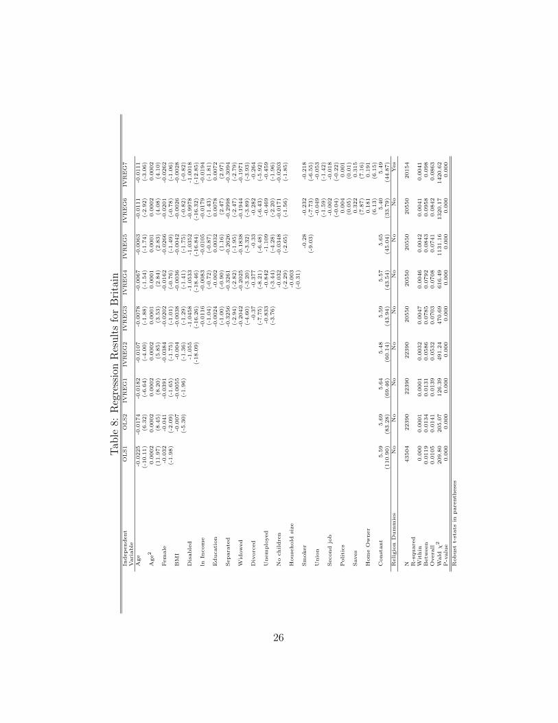
Regressions output for Britain are shown in Table 8. Columns IV REG1 through

IV REG7 present the instrument variable regression results.

The coefficient on BMI has the expected sign. However, except for IV REG1,

the results across specifications are not statistically significant. Life satisfaction

is decreasing with age, at an increasing rate. The results on age are all signifi-

cant. Disability status appears to decrease life satisfaction by 1 whole unit, under

all specifications, a result that is significant at less than 1% level. Surprisingly,

the coefficient on income is negative. However, across specifications IV REG3

through IV REG6 this result is not statistically significant. The results regard-

ing the relationship between education and happiness are not robust. For the

most part, they are not statistically significant, leading to no-single firm conclu-

sion. Being separated, widowed or divorced are all received as negative shocks

to individual life satisfaction. Similar to the German results, being divorced or

separated appears to have the most severe negative impact on personal well be-

ing, among different marital statuses. All marital status results are statistically

12

significant. Smoking appears to negatively affect well being. In particular, under

specifications IV REG5, IV REG6 and IV REG7, the coefficient ranges between

−0.22 and −0.28, significant at the 1% level. Regarding financial information, our

findings indicate that people who save and people who own their own home are

happier, ceteris paribus.

4.3 Results for Australia

The Australian regression results are presented in Table 9. Here, like in the German

data, the regression analysis reveals a negative and highly statistically significant

relationship between BMI and self reported life-satisfaction. In particular, in the

multivariate instrumental variable specifications IV REG4 through IV REG7 the

coefficient on BMI is approximatly −0.04 at the 1% level of significance. Older

age decreases well being, at an increasing rate. Disability is found to lower life

satisfaction slightly more than half a unit, on the 0-10 scale. These findings are

highly statistically significant. As expected, income is associated with higher lev-

els of individual happiness. Individuals with 10% higher income are expected to

report higher levels of life satisfaction of approximately 0.3 units. Educational

attainment has a negative and statistically significant coefficient. Individuals with

more years of education are expected to report a 0.04 lower happiness levels for

every extra year of education they have acquired. With respect to marital status,

individuals who are single, separated, widowed or divorced are expected to report

lower self satisfaction levels than married ones, ceteris paribus. Once again, the

most severe effect appears to come from being separated, where the coefficient is

close to −0.85 under all specifications. The number of children in the Australian

13

regressions does not exhibit statistically significant results, unlike the German and

the British regressions. On the contrary, the size of the household is negatively

related with individual self reported life satisfaction levels. In particular, an one

member difference in the size of a household is expected to result in a 0.07 dif-

ference in the individual happiness levels. The results are significant at the 1%

level.

5 Conclusions

This study investigates the impact of obesity on individual happiness using panel

analysis for Germany, the United Kingdom, and Australia. The contribution to

the literature is three fold: first, to our knowledge, this is the first study to explore

the panel dimension of the existing data in the investigation of the

addressed research question. Secondly, this is the first study that examines

the Australian data to identify the possible relationship between obesity and hap-

piness. In addition, this study addresses the potential endogeneity problems that

arise from most variables included in the specifications used, as a result of reverse

causality. These endogeneity issues are tackled using the panel elements of the

data which offer the necessary exogenous instruments. Last, but not least, we

identify other significant determinants of life-satisfaction and discuss them.

For Germany and Australia, BMI has a negative and statistically significant

relationship with self reported life-satisfaction levels. For Britain, although the

coefficient on BMI is negative in all specifications, the results are not statisti-

cally different from 0. The findings across specifications for all three countries

point to some common conclusions. First, disability severely impacts individual

14

happiness more than any other individual characteristic. Secondly, being sepa-

rated or divorced (compared to being married) reduces well being at a statistically

significant level. Other results indicate that for Germany and Australia income

is positively associated with happiness, as expected. For education, the results

are mixed: for Australia the relationship is negative and significant, whereas for

Germany the opposite holds. For Britain, house ownership and saving habits ap-

pear to be beneficial for individual happiness whereas smoking impairs well being.

Household size, measured as number of people living in a household, decreases life

satisfaction at a statistically significant level, both in Germany and Britain. In

Australia, females appear to be happier whereas in Germany they are found to be

less happy compared to males.

15

References

Blanchflower, D. G. (2008). International Evidence on Well-being. Iza discussion

papers 3354, Institute for the Study of Labor (IZA).

Cameron, C., & Trivedi, P. (2009). Microeconometrics using Stata (1st. edition).,

p. 692. Stata Press.

Cornlisse-Vermatt, J. R., Antonides, G., Ophem, J. V., & den Brink, H. M. V.

(2006). Body Mass Index, Perceived Health, and Happiness: their determi-

nants and structural relationships. Social Indicators Research, 79, 143–158.

Deaton, A., & Arora, R. (2009). Life at to top: the benefits of height. Nber

working papers 15090, National Bureau of Economic Research, Inc. available

at http://ideas.repec.org/p/nbr/nberwo/15090.html.

Frey, B., & Stutzer, A. (2000). Maximising Happiness?. German Economic Review,

1 (2), 145–167.

Frey, B., & Stutzer, A. (2005). Happiness Research: State and Prospects. Review

of Social Economy, 62 (2), 207–228.

Greeno, C., Jackson, C., Williams, E., & Fortmann, S. (1998). The Effect of

Perceived Control over Eating on the Life Satisfaction of Women and Men:

Results from a Community Sample. International Journal of Eating Disor-

ders, 24 (4), 415–419.

Kahneman, D., Diener, E., & Schwarz, N. (1999). Well-being: The Foundations

of Hedonic Psychology, pp. 61–84. Russel Sage Foundation: New York.

16

Larsson, U., Karlsson, J., & Sullivan, M. (2002). Impact of overweight and obesity

on health-related quality of life - a Swedish population study. International

Journal obesity, 26, 417–424.

Needham, B., & Crosnoe, R. (2005). Overweight Status and Depressive Symptoms

During Adolescence. Journal of Adolescent Health, 36 (1), 48–55.

Noppa, H., & Hallstrom, T. (1981). Weight gain in adulthood in relation to

socioeconomic factors, mental illness, and personality traits: a prospective

study of middle-aged women. Journal of Psychosomatic Research, 25, 83–89.

Oswald, A., & Powdthavee, N. (2007). Obesity, Unhappiness, and the Challenge

of Affluence: Theory and Evidence. Economic Journal, 117, F441–F459.

Palinkas, L., Wingard, D., & Barrett-Connor, E. (1996). Depressive symptoms

in overweight and obese older adults: a test of the ”jolly fat” hypothesis.

Journal of Psychosomatic Research, 40, 56–60.

Reed, D. (1985). The relationship between obesity and psychological general well-

being in United States women. Journal of Psychosomatic Research (Ab-

stract), 46, 3791.

Roberts, R., Kaplan, G., Shema, S., & Strawbridge, W. (2000). Are the Obese

at Greater Risk of Depression?. American Journal of Epidemiology, 152 (2),

163–170.

Stutzer, A. (2007). Limited Self-Control, Obesity and the Loss of Happiness. Iza

discussion papers 2925, Institute for the Study of Labor (IZA).

17

Veenhoven, R. (1996). Happy Life-Expectancy. Social Indicators Research, 39,

1–58.

18

Table 1: Descriptive Statistics for German DataGerman Data - GSOEP - Years: 2002, 2004, 2006, 2008

Variable Mean Std. Dev. Min Max Observations

Age overall 46.053 18.242 15 100 N = 180714between 18.923 15 99 n = 33272

within 2.016 41.553 50.553 T-bar = 5.43141

Household size overall 3.023 1.370 1 13 N = 215766between 1.306 1 13 n = 39311

within 0.448 -6.23 9.82 T-bar = 5.48869

No children overall 0.820 1.088 0 9 N = 215766between 1.042 0 7.875 n = 39311

within 0.357 -4.805 4.820 T-bar = 5.48869

Education overall 12.068 2.676 7 18 N = 157209between 2.654 7 18 n = 28833

within 0.331 6.924766 17.21048 T-bar = 5.4524

Life Satisfaction overall 6.964 1.785 0 10 N = 165630between 1.491 0 10 n = 30615

within 1.101 -1.61 14.11 T-bar = 5.41009

Height overall 1.713 0.093 0.82 2.1 N = 83227between 0.092 1.31 2.09 n = 28545

within 0.016 0.96 2.11 T-bar = 2.91564

Weight overall 75.433 15.514 32 230 N = 82681between 15.039 35 200 n = 28452

within 3.962 7.43 156.18 T-bar = 2.90598

BMI overall 25.619 4.589 11.63 197.23 N = 82644between 4.338 12.86 73.46 n = 28449

within 1.556 -20.66 152.64 T-bar = 2.90499

ln Income overall 10.384 0.641 0 15.62 N = 215763between 0.591 0 13.83 n = 39310

within 0.304 0.80 15.82 T-bar = 5.48876

Female overall 0.510 0.500 0 1 N = 215766between 0.500 0 1 n = 39311

within 0.000 0.510 0.510 T-bar = 5.48869

Widowed overall 0.050 0.219 0 1 N = 215766between 0.209 0 1 n = 39311

within 0.063 -0.825 0.925 T-bar = 5.48869

Divorced overall 0.054 0.226 0 1 N = 215766between 0.206 0 1 n = 39311

within 0.087 -0.821 0.929 T-bar = 5.48869

Separated overall 0.013 0.115 0 1 N = 215766between 0.088 0 1 n = 39311

within 0.080 -0.862 0.888 T-bar = 5.48869

Unemployed overall 0.367 0.482 0 1 N = 215766between 0.426 0 1 n = 39311

within 0.247 -0.508 1.242 T-bar = 5.48869

Disabled overall 0.088 0.283 0 1 N = 208742between 0.249 0 1 n = 39030

within 0.120 -0.787 0.963 T-bar = 5.34824

Political party overall 0.448 0.497 0 1 N = 166048member between 0.413 0 1 n = 30638

within 0.297 -0.427 1.323 T-bar = 5.41967

Has a second job overall 0.027 0.162 0 1 N = 166048between 0.118 0.000 1 n = 30638

within 0.120 -0.848 0.902 T-bar = 5.41967

German overall 0.926 0.261 0 1 N = 166048between 0.263 0.000 1 n = 30638

within 0.045 0.0513 1.8013 T-bar = 5.41967

19

Table 2: Correlation Matrix for GSOEP variablesAge Household No children Education Life Height Weight

Size SatisfactionAge 1Household size -0.4380* 1No children -0.3878* 0.7934* 1Education -0.0892* 0.0089* 0.0355* 1Life Satisfaction -0.0631* 0.0670* 0.0460* 0.1370* 1Height -0.2298* 0.0991* 0.0675* 0.1900* 0.0665* 1Weight 0.1055* -0.0102* -0.0170* -0.0005 -0.0348* 0.5266* 1BMI 0.2647* -0.0748* -0.0655* -0.1230* -0.0835* -0.0181* 0.8298*ln Income -0.1515* 0.4198* 0.1791* 0.3403* 0.2179* 0.1650* 0.0253*Female 0.0281* -0.0387* -0.0055* -0.0805* -0.0005 -0.6696* -0.4832*Widowed 0.3583* -0.2648* -0.1574* -0.1325* -0.0471* -0.1921* -0.0493*Divorced 0.0672* -0.1780* -0.0936* -0.0164* -0.0812* -0.0260* -0.0108*Separated 0.0084* -0.0850* -0.0322* 0.0119* -0.0544* 0.0007 -0.0015Not Employed 0.2638* -0.1934* -0.2561* -0.2486* -0.0665* -0.2079* -0.0893*Disabled 0.2815* -0.1875* -0.1849* -0.1025* -0.1618* -0.0564* 0.0708*Political party member 0.1741* -0.0756* -0.0641* 0.1989* 0.1021* 0.0663* 0.0634*Has a second job -0.0567* 0.0150* 0.0112* 0.0455* 0.0145* 0.0300* 0.0037German 0.0698* -0.1210* -0.1009* 0.1703* 0.0272* 0.0814* 0.0284*

BMI ln Income Female Widowed Divorced Separated Not Employed

BMI 1ln Income -0.0784* 1Female -0.1447* -0.0605* 1Widowed 0.0656* -0.2051* 0.1264* 1Divorced 0.002 -0.1438* 0.0372* -0.0551* 1Separated -0.0031 -0.0732* 0.0045* -0.0268* -0.0279* 1Not Employed 0.0332* -0.2330* 0.0907* 0.2285* -0.0284* -0.0259* 1Disabled 0.1182* -0.1104* -0.0277* 0.1092* 0.0371* 0.0093* 0.2117*Political party member 0.0287* 0.1386* -0.0789* 0.0228* -0.0188* -0.0038 -0.0082*Has a second job -0.0144* 0.0288* -0.0061* -0.0280* 0.0144* 0.0118* -0.0799*German -0.0209* 0.0495* 0.0076* 0.0438* 0.0176* -0.0039 -0.0077*

Disabled Political party Has second Germanmember job

Disabled 1Political party member 0.0432* 1Has a second job -0.0269* 0.0177* 1German 0.0234* 0.1299* 0.0048 1

*significant at 5%

20

Table 3: Descriptive Statistics for British DataBritish Data - BHPS - Years: 2005 and 2007



within 1.073 41.46 50.46 T-bar = 3.32451

Household size overall 2.870 1.405 1 14 N = 63038between 1.382 1 13.5 n = 18961

within 0.402 -3.880 8.870 T-bar = 3.32461

No children overall 0.499 0.914 0 7 N = 46800between 0.884 0 7 n = 17675

within 0.182 -1.834 3.166 T-bar = 2.64781

Education overall 11.329 5.052 2 20 N = 28575between 4.999 2 20 n = 15968

within 0.568 2.329 20.329 T-bar = 1.78952


within 0.046 1.05 2.25 T-bar = 1.77287

Weight overall 76.051 15.802 12.7 184.15 N = 23499between 15.969 12.7 184.15 n = 14768

within 2.576 37.05 115.05 T-bar = 1.59121


within 2.316 -74.710 130.560 T-bar = 1.58675

Life Satisfaction overall 5.228 1.280 1 7 N = 58402between 1.104 1 7 n = 18066

within 0.709 0.727852 9.727852 T-bar = 3.2327


within 0.066 -0.215 1.035 T-bar = 3.32461


within 0.061 -0.674 0.826 T-bar = 3.32461


within 0.083 -0.670 0.830 T-bar = 3.32461


within 0.076 -0.729 0.771 T-bar = 3.32461

Unemployed overall 0.032 0.176 0 1 N = 63038between 0.150 0 1 n = 18961

within 0.120 -0.718 0.782 T-bar = 3.32461


within 0.169 -0.672 0.828 T-bar = 3.32461


within 1.009 1.212 15.728 T-bar = 3.29773

Has a second job overall 0.058 0.234 0 1 N = 63038between 0.188 0 1 n = 18961

within 0.147 -0.692 0.808 T-bar = 3.32461

Political party overall 0.264 0.441 0 1 N = 63038member between 0.315 0 1 n = 18961

within 0.309 -0.486 1.014 T-bar = 3.32461

Smoker overall 0.240 0.427 0 1 N = 63038between 0.405 0 1 n = 18961

within 0.148 -0.510 0.990 T-bar = 3.32461

Labor Union overall 0.151 0.358 0 1 N = 63038member between 0.320 0 1 n = 18961

within 0.142 -0.599 0.901 T-bar = 3.32461

Saves overall 0.392 0.488 0 1 N = 63038between 0.390 0 1 n = 18961

within 0.304 -0.358 1.142 T-bar = 3.32461

House Owner overall 0.743 0.437 0 1 N = 63038between 0.425 0 1 n = 18961

within 0.157 -0.007 1.493 T-bar = 3.32461

21

Table 4: Correlation Matrix for BHPS variablesAge Household No children Education Height Weight BMI

sizeAge 1Household size -0.4448 1No children -0.248 0.5744* 1Education 0.3231* -0.0854* -0.1227* 1Height -0.1569 0.0528* 0.014* -0.1488* 1Weight 0.0183* 0.0129* 0.0327* -0.0479* 0.4023* 1BMI 0.1256* -0.0265* 0.0134* 0.0554* -0.2978* 0.7281* 1Life Satisfaction 0.0709* -0.0278* -0.0447* -0.0086 0.0108 -0.0394* -0.0446*Female 0.0233* -0.0176* 0.0317* 0.0556* -0.5426* -0.4119* -0.0701*Widowed 0.4268* -0.2946* -0.1449* 0.2199* -0.1382* -0.0998* -0.0086Divorced 0.0678* -0.1277* -0.0178* 0.0167* -0.0419* 0.0014 0.0307*Separated -0.0125* -0.0453* 0.0397* 0.007 -0.0159* 0.0004 0.0082Unemployed -0.1169* 0.0454* 0.0018 0.0452* 0.0195* -0.0057 -0.0167*Disabled 0.1771* -0.1089* -0.0605* 0.1368* -0.0253* 0.0464* 0.0675*ln Income 0.1984* -0.1433* 0.1413* -0.1935* 0.0614* 0.1622* 0.1161*Has a second job -0.0976* 0.0561* 0.0105* -0.1025* 0.0381* 0.0101 -0.0207*Political party member 0.2346* -0.1067* -0.0833* 0.0618* -0.0107 0.0396* 0.0456*Smoker -0.1386* 0.0362* 0.0523* 0.1264* 0.0087 -0.0706* -0.0731*Labor Union Member -0.0919* 0.0354* 0.0746* -0.2149* 0.0163* 0.0453* 0.0274*Saves -0.0187 -0.0451* -0.0438* -0.1716* 0.0215* 0.0038 -0.0117House Owner 0.0912* 0.0685* -0.0017 -0.1913* 0.0507* 0.0353* -0.0043

Life Female Widowed Divorced Separated Unemployed DisabledSatisfaction

Life Satisfaction 1Female -0.0093 1Widowed 0.0166* 0.1236* 1Divorced -0.0928 0.0563* -0.0842* 1Separated -0.0649 0.022* -0.0416* -0.0428* 1Unemployed -0.0841 -0.0443* -0.0449* 0.0115* 0.0236* 1Disabled -0.1683* 0.0072 0.1001* 0.0615* 0.0094* -0.0295* 1ln Income -0.0124 -0.1207* 0.0325* 0.0686* 0.0412* -0.1133* 0.0004Has a second job 0.0031 0.0011 -0.0551* 0.0074 -0.0056 -0.0066 -0.0599*Political party member 0.0267* -0.0259* 0.0843* -0.0090* -0.0180* -0.0407* 0.0048Smoker -0.1337* -0.0039 -0.0524* 0.0929* 0.0666* 0.1158* 0.0613*Labor Union Member 0.0094* 0.0224* -0.0964* 0.0225* 0.0113* -0.0738* -0.0993*Saves 0.0945* 0.002 -0.0240* -0.0233* -0.0254* -0.0984* -0.0706*House Owner 0.1262* -0.0308* -0.0389* -0.0895* -0.0641* -0.1232* -0.1269*

ln Income Has second Political party Smoker Labor Union Saves House OwnerJob member member

ln Income 1Has a second job -0.0424 1Political party member 0.0764* -0.0135* 1Smoker -0.0032 -0.0031 -0.0529* 1Labor Union Member 0.2040* 0.0339* 0.0152* -0.0361* 1Saves 0.1505* 0.0405* 0.0402* -0.1051* 0.1622* 1House Owner 0.0952* 0.0391* 0.0788* -0.1835* 0.1378* 0.1670* 1

*significant at 5%

22

Table 5: Descriptive Statistics for Australian DataAustralian Data - HILDA - Years: 2006, 2007 and 2009



within 1.320974 38.35421 49.35421 T-bar = 3.91158

Household size overall 3.207649 1.462235 1 14 N = 82649between 1.363177 1 13.5 n = 21265

within 0.657998 -4.99235 10.20765 T-bar = 3.88662

No children overall 1.241713 1.394873 0 14 N = 81787between 1.23369 0 9.6 n = 20736

within 0.747201 -5.95829 12.44171 T-bar = 3.9442

Education overall 11.58874 2.391224 0 18.5 N = 63909between 2.023765 0 18.5 n = 16348

within 1.260333 3.088743 19.58874 T-bar = 3.90929


within 0.022699 1.204411 2.204411 T-bar = 2.08554

Weight overall 76.87511 17.98581 28 260 N = 32870between 17.51675 28 236.6667 n = 14216

within 4.691137 7.541781 160.5418 T-bar = 2.31218


within 1.74933 -38.4166 91.06226 T-bar = 2.06945

Income overall 65529.32 51454.74 1 611361 N = 81902between 42482.27 1 562353 n = 21209

within 30003.61 -354404 474042.1 T-bar = 3.86166


within 2.129551 0.327107 16.8477 T-bar = 3.86166


within 0 0.514283 0.514283 T-bar = 4.19198

Married overall 0.456497 0.498107 0 1 N = 82649between 0.463687 0 1 n = 21265

within 0.174039 -0.3435 1.256497 T-bar = 3.88662

Single overall 0.191339 0.393358 0 1 N = 82649between 0.362321 0 1 n = 21265

within 0.161919 -0.60866 0.991339 T-bar = 3.88662


within 0.055324 -0.75806 0.841936 T-bar = 3.88662


within 0.091528 -0.74794 0.852064 T-bar = 3.88662


within 0.083549 -0.77766 0.822335 T-bar = 3.88662

Not employed overall 0.469455 0.499069 0 1 N = 82649between 0.427514 0 1 n = 21265

within 0.283706 -0.33054 1.269455 T-bar = 3.88662


within 0.204189 -0.64762 0.952379 T-bar = 3.88662

23

Table 6: Correlation Matrix for Australian variablesAge Household No children Education Life Height Weight

Size SatisfactionAge 1Household size -0.3244* 1No children -0.1221* 0.7610* 1Education -0.1421* 0.0273* -0.0693* 1Life Satisfaction 0.0623* 0.0237* -0.0104* -0.0453* 1Height -0.1473* 0.0442* 0.0103 0.0827* -0.01 1Weight 0.0698* 0.0039 0.0380* -0.0063 -0.0350* 0.4728* 1BMI 0.1675* -0.0216* 0.0279* -0.0483* -0.0335* -0.0731* 0.8314*ln Income -0.2022* 0.1604* -0.0986* 0.2714* 0.0498* 0.0643* 0.0230*Female 0.0284* -0.0212* 0.0100* -0.0281* 0.0250* -0.6629* -0.3986*Single -0.5084* -0.0787* -0.1751* -0.0429* -0.0353* 0.0890* -0.1085*Widowed 0.3776* -0.2125* -0.0878* -0.1555* 0.0405* -0.1449* -0.0676*Divorced 0.1353* -0.1736* -0.0575* -0.0258* -0.0804* -0.0558* 0.003Separated 0.0419* -0.0967* -0.0164* -0.0048 -0.0935* -0.0093 0.0126*Not Employed 0.3009* 0.1431* 0.1070* -0.1721* 0.0407* -0.1327* -0.0640*Disabled 0.3188* -0.1988* -0.1197* -0.1732* -0.1582* -0.0751* 0.0586*

BMI ln Income Female Single Widowed Divorced Separated

BMI 1ln Income 0.0012 1Female -0.0570* -0.0489* 1Single -0.1721* -0.0488* -0.0398* 1Widowed 0.0132* -0.1686* 0.1284* -0.1018* 1Divorced 0.0352* -0.0761* 0.0507* -0.1140* -0.0490* 1Separated 0.0160* -0.0333* 0.0126* -0.0735* -0.0316* -0.0354* 1Not Employed 0.0157* 0.1530* 0.0305* -0.1963* 0.1011* -0.0672* -0.0464*Disabled 0.1097* -0.2413* 0.0304* -0.0346* 0.1901* 0.1083* 0.0393*

Not DisabledEmployed

Not Employed 1Disabled 0.0719* 1

*significant at 5%

24

Tab

le7:

RegressionResultsforGerman

yIn

dep

endent

OL

S1

OL

S2

IVR

EG

1IV

RE

G2

IVR

EG

3IV

RE

G4

IVR

EG

5IV

RE

G6

IVR

EG

7V

ari

able

Age

-0.0

164

-0.0

149

0.0

068

0.0

071

-0.0

034

-0.0

086

-0.0

111

-0.0

102

-0.0

114

(-7

.11)

(-5.6

2)

(1.2

2)

(1.4

1)

(-0.4

5)

(-1.1

5)

(-1.2

0)

(-1.3

0)

(-1.3

0)

Age2

0.0

00

0.0

001

-0.0

001

-0.0

001

0.0

00.0

001

0.0

001

0.0

001

0.0

001

(2.0

3)

(2.8

5)

(-2.4

6)

(-2.0

1)

(0.5

9)

(1.2

2)

(1.0

7)

(1.1

1)

(1.0

9)

Fem

ale

0.0

077

-0.0

335

-0.1

132

-0.1

309

-0.0

874

-0.0

915

-0.0

678

-0.0

688

-0.0

726

(0.4

6)

(-1.8

3)

(-3.3

9)

(-5.2

1)

(-3.1

6)

(-2.9

3)

(-1.9

5)

(-2

.35)

(-2.7

5)

BM

I-0

.0141

-0.0

776

-0.0

797

-0.0

739

-0.0

733

-0.0

728

-0.0

74

-0.0

619

(-6.5

8)

(-4.4

4)

(-5.2

9)

(-4.9

8)

(-4.0

7)

(-3.8

1)

(-4.3

8)

(-4.1

2)

Dis

able

d-0

.5352

-0.5

667

-0.5

889

-0.6

031

-0.5

99

-0.5

985

(-13.2

)(-

13.3

2)

(-15.9

)(-

14.3

1)

(-15.3

9)

(-15.5

5)

lnIn

com

e0.3

232

0.4

557

0.4

166

0.4

127

0.4

208

(7.6

9)

(8.2

9)

(7.1

3)

(7.6

3)

(7.8

9)

Educati

on

0.0

472

0.0

353

0.0

238

0.0

249

0.0

316

(9.5

8)

(5.4

1)

(4.2

8)

(4.9

4)

(6.3

6)

Separa

ted

-0.1

277

-0.1

886

-0.2

155

-0.2

127

-0.2

263

(-1.6

0)

(-1.9

4)

(-1.8

5)

(-1.6

6)

(-1.6

6)

Wid

ow

ed

0.0

965

0.0

20.0

17

0.0

227

0.0

582

(1.7

4)

(0.3

6)

(0.2

7)

(0.3

6)

(0.9

0)

Sin

gle

-0.1

182

-0.1

423

-0.1

543

-0.1

503

-0.1

443

(-3.2

6)

(-3.9

4)

(-3.9

4)

(-4.0

7)

(-4.0

4)

Div

orc

ed

-0.2

438

-0.2

94

-0.2

993

-0.2

954

-0.2

603

(-5.1

6)

(-5.9

9)

(-6.0

4)

(-5.0

9)

(-4.5

7)

Not

em

plo

yed

0.0

199

0.0

534

0.0

435

0.0

441

0.0

418

(0.5

7)

(1.6

6)

(1.0

5)

(1.1

9)

(0.9

7)

No

childre

n0.0

935

0.0

852

0.0

84

0.0

873

(5.3

0)

(5.0

7)

(4.3

3)

(4.2

5)

House

hold

size

-0.1

188

-0.1

052

-0.1

041

-0.1

067

(-4.9

1)

(-4.6

0)

(-4.6

9)

(-4.7

9)

Second

job

0.2

368

0.2

379

0.2

26

(1.5

1)

(1.7

9)

(1.5

2)

Politi

cs

0.3

678

0.3

707

0.2

973

(8.7

5)

(8.8

9)

(5.2

0)

Germ

an

-0.0

641

-0.1

006

(-1.4

3)

(-1.9

7)

Const

ant

7.6

37.8

38.9

68.9

95.0

64.2

54.6

64.7

64.4

9(1

51.6

5)

(112.3

6)

(27.4

3)

(32.5

8)

(9.0

6)

(6.9

9)

(6.2

2)

(6.9

3)

(7.4

3)

Religio

nD

um

mie

sN

oN

oN

oN

oN

oN

oN

oN

oY

es

N165630

82466

82466

82423

70287

70287

70247

70247

65338

R-s

quare

dW

ithin

0.0

103

0.0

007

0.0

00

0.0

001

0.0

005

0.0

008

0.0

014

0.0

013

0.0

017

Betw

een

0.0

089

0.1

21

0.0

121

0.0

285

0.0

778

0.0

868

0.0

94

0.0

929

0.1

21

Overa

ll0.0

044

0.0

075

0.0

078

0.0

194

0.0

555

0.0

624

0.0

668

0.0

66

0.0

81

Wald

χ2

692.6

3377.5

5349.3

4614.0

81339.9

61549.5

21866.6

12366.1

92455.4

2P

-valu

e0.0

00

0.0

00

0.0

00

0.0

00

0.0

00

0.0

00

0.0

00

0.0

00

0.0

00

Robust

t-st

ats

inpare

nth

ese

s

25

Tab

le8:

RegressionResultsforBritain

Indep

endent

OL

S1

OL

S2

IVR

EG

1IV

RE

G2

IVR

EG

3IV

RE

G4

IVR

EG

5IV

RE

G6

IVR

EG

7V

ari

able

Age

-0.0

225

-0.0

174

-0.0

182

-0.0

107

-0.0

078

-0.0

067

-0.0

063

-0.0

111

-0.0

111

(-10.1

1)

(6.3

2)

(-6.6

4)

(-4.0

0)

(-1.8

8)

(-1.5

4)

(-1.7

4)

(-2.9

2)

(-3.0

6)

Age2

0.0

002

0.0

002

0.0

002

0.0

002

0.0

001

0.0

001

0.0

001

0.0

002

0.0

002

(11.9

7)

(8.4

5)

(8.2

0)

(5.8

5)

(3.5

3)

(2.8

4)

(2.8

3)

(4.0

8)

(4.1

0)

Fem

ale

-0.0

32

-0.0

41

-0.0

391

-0.0

384

-0.0

202

-0.0

162

-0.0

266

-0.0

201

-0.0

262

(-1.9

8)

(-2.0

9)

(-1.6

5)

(-1.7

5)

(-1.0

1)

(-0.7

6)

(-1.4

9)

(-0.7

8)

(-1.0

6)

BM

I-0

.007

-0.0

055

-0.0

04

-0.0

038

-0.0

036

-0.0

042

-0.0

026

-0.0

028

(-5.3

0)

(-1.9

6)

(-1.3

6)

(-1.2

9)

(-1.4

1)

(-1.7

5)

(-0.8

2)

(-0.8

2)

Dis

able

d-1

.055

-1.0

458

-1.0

533

-1.0

352

-0.9

978

-1.0

018

(-18.0

9)

(-16.2

6)

(-18.4

6)

(-16.8

4)

(-16.3

2)

(-12.8

5)

lnIn

com

e-0

.0116

-0.0

083

-0.0

105

-0.0

179

-0.0

194

(-1.0

4)

(-0.7

2)

(-0.8

7)

(-1.4

3)

(-1.8

1)

Educati

on

-0.0

024

-0.0

02

0.0

032

0.0

078

0.0

072

(-1.0

0)

(-0.9

0)

(1.1

6)

(2.4

7)

(2.9

7)

Separa

ted

-0.3

256

-0.3

261

-0.2

626

-0.2

998

-0.3

094

(-2.9

4)

(-2.8

2)

(-1.9

5)

(-2.4

7)

(-2.7

9)

Wid

ow

ed

-0.2

042

-0.2

025

-0.1

838

-0.1

944

-0.1

971

(-4.6

0)

(-3.2

0)

(-3.3

2)

(-3.8

9)

(-3.9

3)

Div

orc

ed

-0.3

7-0

.377

-0.3

3-0

.282

-0.2

64

(-7.7

5)

(-8.2

1)

(-6.4

8)

(-6.4

3)

(-5.9

2)

Unem

plo

yed

-0.8

33

-0.8

42

-1.1

09

-0.4

69

-0.4

59

(-3.7

6)

(-3.4

4)

(-4.2

8)

(-2.2

0)

(-1.9

6)

No

childre

n-0

.032

-0.0

348

-0.0

171

-0.0

203

(-2.2

9)

(-2.6

5)

(-1.5

6)

(-1.8

5)

House

hold

size

-0.0

03

(-0.3

1)

Sm

oker

-0.2

8-0

.232

-0.2

18

(-9.0

3)

(-7.7

3)

(-6.5

5)

Unio

n-0

.049

-0.0

53

(-1.5

9)

(-1.4

2)

Second

job

-0.0

02

-0.0

18

(-0.0

4)

(-0.2

2)

Politi

cs

0.0

04

0.0

01

(0.0

5)

(0.0

1)

Saves

0.3

22

0.3

15

(7.8

7)

(7.1

6)

Hom

eO

wner

0.1

81

0.1

91

(6.1

3)

(6.1

5)

Const

ant

5.5

95.6

95.6

45.4

85.5

95.5

75.6

55.4

05.4

9(1

10.9

0)

(83.2

8)

(69.4

6)

(60.1

4)

(43.9

4)

(43.5

4)

(45.0

4)

(33.7

9)

(44.8

7)

Religio

nD

um

mie

sN

oN

oN

oN

oN

oN

oN

oN

oY

es

N43504

22390

22390

22390

20550

20550

20550

20550

20154

R-s

quare

dW

ithin

0.0

00

0.0

001

0.0

001

0.0

032

0.0

047

0.0

046

0.0

042

0.0

041

0.0

041

Betw

een

0.0

119

0.0

134

0.0

131

0.0

586

0.0

785

0.0

792

0.0

843

0.0

958

0.0

98

Overa

ll0.0

105

0.0

141

0.0

139

0.0

532

0.0

703

0.0

708

0.0

741

0.0

842

0.0

863

Wald

χ2

209.8

0205.0

7126.3

9491.2

4470.6

9616.4

91131.1

61320.1

71420.6

2P

-valu

e0.0

00

0.0

00

0.0

00

0.0

00

0.0

00

0.0

00

0.0

00

0.0

00

0.0

00

Robust

t-st

ats

inpare

nth

ese

s

26

Tab

le9:

RegressionResultsforAustralia

Indep

endent

OL

S1

OL

S2

IVR

EG

1IV

RE

G2

IVR

EG

3IV

RE

G4

IVR

EG

5IV

RE

G6

IVR

EG

7V

ari

able

Age

-0.0

42

-0.0

44

-0.0

33

-0.0

34

-0.0

34

-0.0

37

-0.0

36

-0.0

36

-0.0

39

(-13.2

6)

(-17.7

8)

(-7.8

2)

(-8.1

0)

(-5.8

5)

(-3.9

4)

(-4.3

1)

(-4.2

3)

(-5.5

2)

Age2

0.0

005

0.0

005

0.0

004

0.0

005

0.0

005

0.0

005

0.0

05

0.0

005

0.0

005

(15.5

4)

(19.5

)(1

1.0

1)

(11.5

5)

(8.4

1)

(5.3

7)

(6.1

1)

(5.9

9)

(6.9

8)

Fem

ale

0.0

44

0.0

58

0.0

36

0.0

36

0.0

63

0.0

62

0.0

61

0.0

60

0.0

69

(1.8

7)

(2.9

1)

(1.6

4)

(1.5

9)

(2.4

9)

(2.4

5)

(1.8

9(2

.64)

(2.5

5)

BM

I-0

.005

-0.0

3-0

.0306

-0.0

439

-0.0

409

-0.0

412

-0.0

412

-0.0

37

(-2.2

7)

(-2.7

4)

(-2.6

6)

(-3.0

4)

(-2.1

6)

(-2.5

3)

(-2.1

0)

(-2.2

1)

Dis

able

d-0

.570

-0.5

24

-0.5

33

-0.5

31

-0.5

31

-0.5

34

(-15.8

)(-

12.4

6)

(-8.4

1)

(-11.1

9)

(-9.6

5)

(-8.5

9)

lnIn

com

e0.2

32

0.3

26

0.3

11

0.3

11

0.3

49

(3.5

2)

(2.1

3)

(2.7

6)

(3.2

8)

(2.5

3)

Educati

on

-0.0

36

-0.0

41

-0.0

41

-0.0

40

-0.0

34

(-6.7

3)

(-4.7

6)

(-5.5

7)

(-6.3

3)

(-4.0

3)

Sin

gle

-0.2

41

-0.2

71

-0.2

83

-0.2

82

-0.2

60

(-4.5

5)

(-5.1

3)

(-5.3

0)

(-5.5

4)

(-5.3

5)

Separa

ted

-0.8

26

-0.8

75

-0.8

53

-0.8

53

-0.8

50

(-4.9

9)

(-6.2

8)

(-5.4

7)

(-5.4

7)

(-5.0

3)

Wid

ow

ed

-0.1

98

-0.2

41

-0.2

14

-0.2

14

-0.1

89

(-2.4

6)

(-2.5

6)

(-2.3

8)

(-2.5

7)

(-2.1

4)

Div

orc

ed

-0.3

26

-0.3

72

-0.3

58

-0.3

58

-0.3

27

(-3.9

5)

(-5.6

4)

(-4.7

8)

(-5.4

2)

(-4.2

6)

Not

Em

plo

yed

0.1

32

0.2

135

0.2

21

0.2

21

0.2

17

(1.6

0)

(1.7

8)

(2.3

1)

(2.3

4)

(1.6

9)

No

childre

n0.0

53

(0.9

7)

House

hold

size

-0.1

04

-0.0

68

-0.0

68

-0.0

74

(-1.4

7)

(-2.3

5)

(-2.7

8)

(-2.1

6)

Const

ant

8.6

88.6

39.2

19.2

07.4

76.7

76.8

66.8

66.2

9(1

12.1

9)

(161.2

)(3

8.8

4)

(37.6

4)

(8.4

4)

(4.1

4)

(5.4

6)

(5.6

7)

(4.0

2)

Regio

nal

Dum

mie

sN

oN

oN

oN

oN

oN

oN

oN

oY

es

N51209

21887

21887

21887

19739

19739

19739

19739

19739

R-s

quare

d

Wit

hin

0.0

00

0.0

03

0.0

013

0.0

013

0.0

045

0.0

047

0.0

048

0.0

048

0.0

047

Betw

een

0.0

283

0.0

267

0.0

583

0.0

583

0.0

708

0.0

697

0.0

695

0.0

696

0.0

777

Overa

ll0.0

212

0.0

253

0.0

495

0.0

495

0.0

619

0.0

614

0.0

614

0.0

614

0.0

677

F105.2

329.7

873

Wald

χ2

427.1

5352.0

9714.4

11053.3

2882.2

9839.9

61089.3

21104.0

61574.6

1P

-Valu

e0.0

000

0.0

000

0.0

000

0.0

000

0.0

000

0.0

000

0.0

000

0.0

000

0.0

000

Robust

t-st

ats

inpare

nth

ese

s

27

Disclaimer

This paper uses unit record data from the Household, Income and Labour Dynamics in Australia (HILDA) Survey.

The HILDA Project was initiated and is funded by the Australian Government Department of Families, Housing,

Community Services and Indigenous Affairs (FaHCSIA) and is managed by the Melbourne Institute of

Applied Economic and Social Research (Melbourne Institute). The findings and views reported in this paper,

however, are those of the author and should not be attributed to either FaHCSIA or the Melbourne Institute.

The data used in this publication was made available to us by the German Socio-Economic Panel Study (SOEP)

at the German Institute for Economic Research (DIW Berlin), Berlin.

28

obesity and happiness - central web server 2 - uits...

Documents