obesity and the labor market: a fresh look at the weight ...ftp.iza.org/dp7947.pdf · obesity and...
TRANSCRIPT
DI
SC
US
SI
ON
P
AP
ER
S
ER
IE
S
Forschungsinstitut zur Zukunft der ArbeitInstitute for the Study of Labor
Obesity and the Labor Market:A Fresh Look at the Weight Penalty
IZA DP No. 7947
February 2014
Marco CaliendoMarkus Gehrsitz

Obesity and the Labor Market:
A Fresh Look at the Weight Penalty
Marco Caliendo University of Potsdam,
IZA, DIW Berlin and IAB Nuremberg
Markus Gehrsitz City University of New York
Discussion Paper No. 7947 February 2014
IZA
P.O. Box 7240 53072 Bonn
Germany
Phone: +49-228-3894-0 Fax: +49-228-3894-180
E-mail: [email protected]
Any opinions expressed here are those of the author(s) and not those of IZA. Research published in this series may include views on policy, but the institute itself takes no institutional policy positions. The IZA research network is committed to the IZA Guiding Principles of Research Integrity. The Institute for the Study of Labor (IZA) in Bonn is a local and virtual international research center and a place of communication between science, politics and business. IZA is an independent nonprofit organization supported by Deutsche Post Foundation. The center is associated with the University of Bonn and offers a stimulating research environment through its international network, workshops and conferences, data service, project support, research visits and doctoral program. IZA engages in (i) original and internationally competitive research in all fields of labor economics, (ii) development of policy concepts, and (iii) dissemination of research results and concepts to the interested public. IZA Discussion Papers often represent preliminary work and are circulated to encourage discussion. Citation of such a paper should account for its provisional character. A revised version may be available directly from the author.

IZA Discussion Paper No. 7947 February 2014
ABSTRACT
Obesity and the Labor Market: A Fresh Look at the Weight Penalty*
This paper applies semiparametric regression models to shed light on the relationship between body weight and labor market outcomes in Germany. We find conclusive evidence that these relationships are poorly described by linear or quadratic OLS specifications, which have been the main approaches in previous studies. Women’s wages and employment probabilities do not follow a linear relationship and are highest at a body weight far below the clinical threshold of obesity. This indicates that looks, rather than health, is the driving force behind the adverse labor market outcomes to which overweight women are subject. Further support is lent to this notion by the fact that wage penalties for overweight and obese women are only observable in white-collar occupations. On the other hand, bigger appears to be better in the case of men, for whom employment prospects increase with weight, albeit with diminishing returns. However, underweight men in blue-collar jobs earn lower wages because they lack the muscular strength required in such occupations. JEL Classification: J31, J71, C14 Keywords: obesity, wages, employment, semiparametric regression, gender differences Corresponding author: Markus Gehrsitz City University of New York Graduate Center 365 5th Avenue New York, NY, 10016 USA E-mail: [email protected]
* The authors thank Karina Doorley, Anne Gielen, Michael Grossman, David Jaeger, Wim Vijverberg and the participants of the CUNY dissertation seminar and the 2013 EALE annual conference for helpful comments.

1 Introduction
The more you weigh, the less you make. A negative association between body weight and
wages is well established in the labor economics literature. It has been observed in the
United States (Averett and Korenman, 1996; Cawley, 2004; Conley and Glauber, 2006,
among others), as well as in European countries such as Denmark (Greve, 2008), England
(Morris, 2006), Finland (Johansson, Backerman, Kiiskinen, and Helivaara, 2009), France
(Paraponaris, Saliba, and Ventelou, 2005), Germany (Cawley, Grabka, and Dean, 2005),
Sweden (Lundborg, Nystedt, and Rooth, 2010), and even in Taiwan (Tao, 2008).
Higher weight is not only associated with drawbacks for those in employment, but
also for those searching for a job. Chubby job seekers have considerably lower chances of
initially finding a job than their slimmer, equally qualified peers (Lindeboom, Lundborg,
and van der Klaauw, 2010; Garcia and Quintana-Domeque, 2006, among others) and
certain jobs are not even open to overweight applicants (Cawley and Maclean, 2012). Obese
unemployed are forced to spend more time on welfare (Cawley and Danziger, 2005). In
addition, being overweight has adverse effects on those who already face obstacles in the
job market. For instance, heavy women tend to be more prone to adverse labor market
outcomes than overweight men (Mocan and Tekin, 2011). There is also evidence that they
have less success in their transition back to employment, despite putting in more effort
and having lower reservation wages (Caliendo and Lee, 2013).
Despite a plethora of research on the relationship between body weight and labor mar-
ket outcomes, such studies usually do not consider heterogeneous and non-linear effects.
Most studies simply apply linear or dummy variable regressions of wages on body weight.
Recent studies by Gregory and Ruhm (2011) for the US and a European cross-country
analysis by Hildebrand and Van Kerm (2010) indicate functional form errors in these
specifications. Consequently, past studies most likely failed to uncover the true association
between wages and body weight; moreoever, they also did not account for heterogeneity
across different occupational categories. Based on data from the German Socio-Economic
Panel, our study remedies these issues in two ways. First, we apply a semiparametric model
that allows for a flexible functional form. Second, we divide our sample into blue-collar and
white-collar workers, distinguishing between occupations in which physical attractiveness
is productivity-enhancing and those where it is not. To the best of our knowledge, we are
also the first to apply a semiparametric model to gain insights on the relationship between
2

employment and body weight.
Our results indicate looks-based discrimination against women in terms of lower wages,
albeit only in white-collar jobs. Even women of normal weight are subject to wage penal-
ties, and thus it might be misleading to refer to this effect as an “obesity penalty”. Our
analysis also suggests that what at first glance appears to be looks-based discrimination
against underweight men more likely results from a lack of fitness and strength, which tend
to be of particular importance in blue-collar jobs. Our results are robust to the inclusion
of controls for muscle strength and to the use of alternative measures of body composition,
namely fat-free mass and body fat. They also hold when we further stratify our sample by
job type. Altogether, we find a level of heterogeneity, which partly confirms the findings
of previous studies, but also shows them in a different complexion.
We also find that the employment probability peaks for women way before the clinical
threshold of obesity is reached. On the other hand, a parametric probit model would have
suggested continuously declining employment probabilities in body weight. For men, we
find that the propensity for employment peaks at a body weight that is actually quite
close to the obesity threshold.
The remainder of the paper is organized as follows. Section 2 describes the data used
and presents first descriptive evidence on the outcomes of interest. In Section 3, we discuss
our methodological approach before presenting the results in Section 4. Finally, Section 5
concludes and provides an outlook for further research.
2 Data
We use data from the German Socio-Economic Panel (GSOEP) as the basis for our anal-
ysis. The GSOEP is an annual panel survey that follows around 22,000 individuals from
12,000 different households across Germany. Each wave draws a representative sample of
the overall German population. Our sample consists of the 2002, 2004, 2006, and 2008
waves of the survey, during which information on both body weight and height was ob-
tained from all participants. From this information, we construct each respondent’s Body
Mass Index (BMI) as the main explanatory variable of our study. BMI is the most com-
monly used measure of obesity (see Burkhauser and Cawley, 2008, for a discussion of the
merits and demerits of using this measure). It is defined as an adult’s weight in kilograms
divided by the square of his or her height in meters. The World Health Organization
3

(WHO) deems individuals with a BMI between 20 and 25 as having a healthy “normal”
weight. Individuals with a BMI higher than 30 are classified as obese, while those with a
BMI between 25 and 30 are rated as overweight (WHO, 2000). Obesity and, to a lesser
degree, being overweight, is significantly associated with poor health and higher mortal-
ity in general (Allison, Fontaine, Manson, Stevens, and VanItallie, 1999), and diabetes,
high cholesterol, and high blood pressure in particular (Mokdad, Ford, Bowman, Dietz,
Bales, and Marks, 2003). Obesity is also one of the main causes for rising health care costs
(Cawley and Meyerhoefer, 2012).
Height and weight are self-reported in the GSOEP. Previous studies, e.g. Cawley
(2004), tried to correct potential reporting error by applying a method developed by
Bound, Brown, and Mathiowetz (2001), which relies on measured weight and height of
participants of the National Health and Nutrition Examination Survey (NHANES III).
We refrain from adjusting our BMI measure since we have no such benchmark study avail-
able for Germany, and the merits of this method are not beyond doubt (Han, Norton, and
Stearns, 2009). However, we drop respondents reporting implausible weight or height, as
well as those for whom height or weight were imputed. We also drop persons with severe
disabilities from our analysis.
The dependent variable in our wage specification is the hourly wage rate, which is con-
structed from the reported weekly earnings and hours of work. We also adjust wages from
different waves for inflation. Respondents who claim to have hourly wages that exceed
e300 or lie below e2 are not considered in our analysis. Naturally, we only observe wages
for respondents who are in employment. Due to this selection issue, our results should
be interpreted as lower bound estimates. Moreoever, we focus on the prime-age employ-
ment body and therefore exclude pensioners, military personnel, and respondents who are
currently attending school or college, or undertake an apprenticeship or traineeship. We
only include employees who work at least 20 hours per week in our wage regression. As
indicated above, bodyweight might also affect a person’s employment prospects and thus
the ability to earn positive wages in the first place. Therefore, we also run a regression of
employment on bodyweight. Our dependent variable is a dummy that adopts a value of
1 if a person is employed or self-employed, and works at least 1 hour per week, and zero
otherwise.
Insert Table 1 about here
4

In order to avoid data issues pertaining to retirement and schooling, we limit our
analysis to persons between the ages of 20 and 60. We pool data from different waves,
but only use the most recent observation for each respondent. Our final sample comprises
8,770 men and 9,229 women.
The average BMI in our sample is 24.45 for women and 26.13 for men (see Table 1).
Almost 60 percent of the men in our sample are either overweight or obese, compared
to a little more than one-third of women. Our descriptive statistics do not show any
considerable differences between overweight and normal weight women in terms of either
hourly wage rate or employment prospects.
For overweight men, hourly wages are on average around 80 euro cents higher than for
average weight men. 87 percent of men with a BMI higher than 25 are in employment,
as opposed to 76 percent of men with a BMI smaller than 25. Moreoever, overweight and
obese respondents on average rate their own health worse than normal weight respondents.
Of course, such simple mean comparisons fail to take the effect of other observable variables
into account. For instance, obesity is more prevalent in older workers, who also tend to be
less healthy and have more lifetime work experience. Our regressions, both parametric and
nonparametric, take this into account, yielding coefficients that have the familiar ceteris
paribus interpretation.
Throughout our empirical analysis, we control for educational attainment, parental
education, marital status, country of origin, the number of children in the household and
their age, as well as work experience and its square. This is important as obesity has been
shown to be associated with socio-economic factors that might also affect wages (Baum
and Ruhm, 2009; Strulik, 2014). We also include dummies for different age categories, a
respondent’s region of residence, and the wave to which an observation pertains. Controls
for whether a person works in a white- or blue-collar job, and has supervision duties or
holds a higher management position are also included, as is a set of dummies indicating the
self-reported health status. We also created measures of personality traits such as openness,
extraversion, neuroticism, agreeableness, reciprocity, self-esteem, and impulsivity. Most
of these measures turned out to be neither jointly nor individually significant and were
therefore not used for our analysis.
5
3 Methodology
Our main tool of analysis is a generalized additive model (GAM) that allows for a semi-
parametric estimation of a regression model of the following form:
Yi = Xiβ + f(BMIi) + εi (1)
where Yi is the log of hourly wages of person i in our wage regression and an employ-
ment status dummy in our analysis of employment prospects. Our explanatory variable of
interest, BMIi, enters the model in a non-parametric fashion, whereas we assume a lin-
ear, parametric functional form for our control variables. This provides for a more flexible
functional form that allows us to accommodate effect patterns that cannot be observed
by simple linear regressions, even if they include quadratic or cubic terms.
Estimation is based on the backfitting algorithm described by Hastie and Tibshirani
(1990) and explained in detail in Keele (2008). This approach involves an iterative process,
based on partial residuals. We use β0 = Y and fj = Xj for all j, as starting values, which
are collected in matrix Sj. In a first step, partial residuals are obtained for each variable
using these starting values. For instance, epX1 is obtained as ep
X1 = Yj −∑k
j=2 Sj − Y . In
a second step, each partial residual is regressed on the corresponding X-column. That is
epX1 is regressed on X1, ep
X2 is regressed on X2, etc.. The resulting coefficients are used to
update matrix Sj, before the iteration starts over with step one. The procedure is repeated
until the model converges in terms of infinitesimally small changes in the residual sum of
squares. In a linear parametric setting the coefficients obtained using this iterative process
will be the usual least squares estimates. In a semiparametric setting, the regression in step
two is fitted using a smoother. More precisely, we use penalized cubic regression splines
to smooth the estimated residuals on the BMI variable.
The smoothing parameter, which determines the number of knots, is chosen via gener-
alized cross-validation (GCV). Loader (1999) points out that such automated smoothing,
whereby the analysts do not have any control over the selection of the smoothing pa-
rameter, can lead to overfitting in some instances. Accordingly, he suggests adjusting the
smoothing parameter using visual analysis. For our study, this turns out not to be neces-
sary, given that overfitting is not an issue. To show this, we included a graph where we
manually chose the bandwidth by rounding the bandwidth parameter yielded by GCV
6

up to its closest integer, alongside the graph yielded by GCV (see Figures 1 and 2). The
differences between regressions with automated (GCV) bandwith selection and manual –
some might argue – arbitrary bandwidth selection are negligible. Neither approach yielded
patterns with large spikes or other irregularities. If anything, the GCV algorithm leads to
slightly more conservative estimates of the relationship between wages and BMI. For the
employment models that have a binary dependent variable, the same backfitting algorithm
can be used in the context of an iterated, reweighed least squares regression, as outlined
in Wood (2006).1
A methodological concern that is often mentioned in the context of our research ques-
tion is variable endogeneity. Both potential reverse causality and omitted relevant vari-
ables might bias our estimates. The most common strategy to deal with this problem is
an instrumental variable regression. In this respect, a genetic predisposition (Norton and
Han, 2008; Cawley, Han, and Norton, 2011) or the weight of family members (Brunello
and D’Hombres, 2007, among others) is often used as an instrument. Proponents of this
strategy cite an adoption study by Grilo and Poguegeile (1991) that appears to show
no correlation between a common household environment and household members’ BMI.
However, considering that family members share a common socio-economic environment,
the validity of such an instrument is not beyond doubt. Given the focus of our paper on
bias caused by a misspecification of the functional form, we therefore deliberately refrain
from applying the instrumental variable technique. Consequently, the results of this paper
should not be interpreted as fully causal effects.
4 Empirical Results
Our empirical analysis consists of the following steps. In order to render our work com-
parable to others, we first run an OLS regression of log hourly wages on BMI. However,
unlike many previous studies, we do not stop at this point. Instead, in a second step, we
apply a semiparametric model to investigate whether the linear functional form masks im-
portant details about the relationship of interest. Third, we combine the semiparametric
setup with stratification techniques in order to better isolate the channel through which
bodyweight affects wages. Furthermore, we also subject our results to several robustness
1The estimations were conducted using the mgcv package in R, which also calculates bias-adjustedvariance-covariance matrices from which confidence bands can be derived.
7

checks. Finally, we also apply a semiparametric model to gain a better understanding
about the relationship between bodyweight and employment.
4.1 Bodyweight and Wages - Parametric Model Results
A regular, parametric OLS regression model of women’s log-wages on the BMI variable
indicates that a 1 point increase in BMI is associated with a decrease in wages of around 0.6
percent (see column (1) of Panel A in Table 2). This effect is highly significant and robust
to the inclusion of controls for health and a standard-set of socio-economic variables. In a
specification in which BMI enters the regression equation both linearly and quadratically,
neither coefficient is statistically significant. At first glance, all signs point to a linear
relationship between BMI and hourly wages of about the same magnitude as has been
found in other countries.2
Insert Table 2 about here
Our OLS-findings for men are also very much in line with previous studies, which
usually arrive at the result that men are not subject to any weight penalties or premiums
in the labor market (Baum and Ford, 2004, among others). The BMI coefficient in our
linear OLS specification is not statistically significant (see Panel B in Table 2), while the
coefficients in our quadratic specification are barely statistically significant (p-values< 0.1).
4.2 Bodyweight and Wages - Semiparametric Model Results
It initially appears that, similar to the findings for other countries, women in Germany are
subject to an obesity wage penalty, whereas men are not. However, our semiparametric
model of the form of equation (1) shows that a linear functional form fails to uncover
important details.
Insert Tables 3 and 4 about here
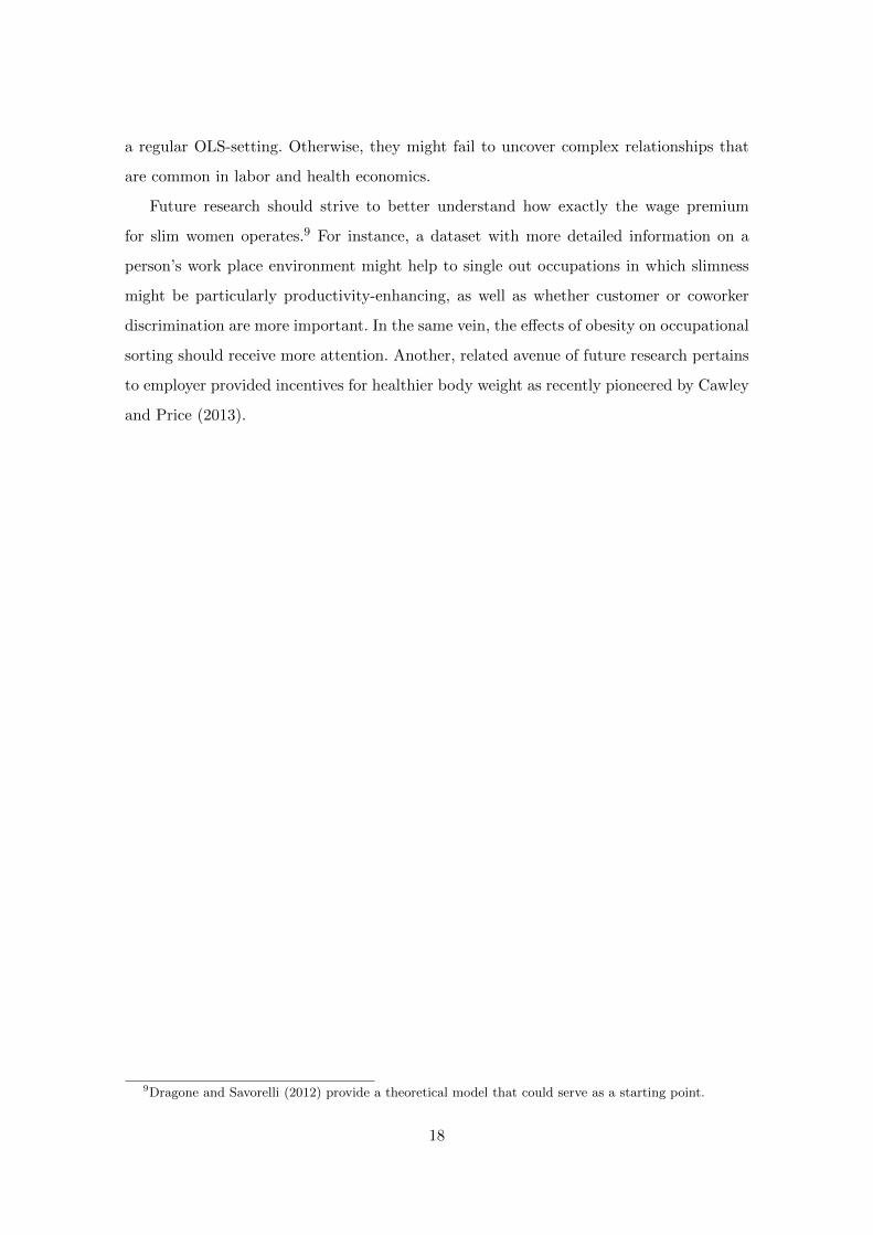
First, note that the coefficients for the control variables are as expected (see Tables 3
and 4). For instance, college graduates earn higher wages, and log wages increase in age up
to a point, while bad health is associated with adverse labor market outcomes. Naturally,
2To the best of our knowledge, Cawley, Grabka, and Dean (2005) have conducted the only nation-ally representative study on the relationship between physical characteristics and earnings in Germany.However, they did not analyse the effect of body weight on hourly wages or employment.
8

we cannot report any coefficients for our main explanatory variable, BMI, as it enters the
model nonparametrically.
Therefore, it should be interpreted graphically, using Figure 1 for women and Figure
2 for men. Our model indicates that women’s wages peak at a BMI of around 21.5, and
steadily decrease for higher body weight. This early peak is not consistent with the notion
of an obesity wage penalty due to health constraints. In fact, there appears to be no penalty
for obesity, but rather a wage premium for slim women. The size of these effects is also not
negligible. The wage gap between the peak and the region where the relationship starts to
level out amounts to around 12 percent. This effect cannot be attributed to health effects,
given that we control for self-reported health. All this suggests that physical appearance
is the driving force behind our results, as female slimness is generally deemed as attractive
(Stearns, 2002).
Insert Figure 1 about here
For men, a regular OLS model also fails to uncover important details. Figure 2 provides
evidence for wage penalties against men who are deemed too light. Wages then peak on a
plateau that ranges from around BMI=23 well into a BMI range in which individuals are
considered overweight or even obese. At first glance, one might suspect that men are simply
held to different beauty standards. Obesity is not punished in terms of lower wages, but
rather underweight men are. In fact, even men in the lower bounds of the normal weight
range are subject to wage penalties. Such a result is consistent with previous findings, and
is commonly referred to as the “portly banker” effect (Cawley, 2004), i.e. the notion that
higher weight might reflect power and authority. Consequently, underweight men might
lack such an aura. This explains wage differences of 7-8 percent between underweight men
and those with BMIs within the forementioned plateau range.
Insert Figure 2 about here
Moreoever, the likelihhod ratio tests for the specifications for both men and women
suggest that our semiparametric regressions differ significantly from parametric linear or
quadratic setups (see p-values in bottom row of Table 2). Accordingly, it required the
flexibel functional form of our semiparametric model to uncover the true relationship
between hourly wages and bodyweight.
9

4.3 Bodyweight and Wages - Stratification Results
The previous section has already hinted that physical attractiveness is the main channel
through which bodyweight affects female wages. We find further support for this hypothesis
by stratifying our sample by occupational type. Looks tend to be more important in white-
collar occupations, within which employees interact with customers and coworkers more
frequently. There is some evidence that good looks might be an asset in such circumstances
(Hamermesh and Parker, 2005, among others). On the other hand, beauty is presumably
less important in blue-collar occupations.
Our results suggest that the previously described pattern more-or-less holds for women
in white-collar occupations (see bottom left of Figure 1), but not for women in blue-collar
jobs. That is, wages for women in white-collar occupations peak at a BMI of about 22
and subsequently decrease in body weight. The semiparametric specification statistically
significantly differs from both a linear and quadratic specification (see p-values for the
LR-Test in the bottom row of Panel A in Table 2), which consequently fail to detect the
same pattern.
For women in blue-collar jobs, the semiparametric results resemble the results of a
linear regression model. In fact, our backfitting algorithm suggests a linear fit. Even if we
manually force some non-linearity on the regression, the resulting line has little curvature
(see bottom right of Figure 1). A likelihood ratio test also fails to reject the hypothesis
that the parametric and semiparametric model come to the same result at any reasonable
significance level. That is, higher bodyweight is strictly negatively associated with wages
in blue-collar jobs.3
Stratification by occupational category also provides further insights regarding the
apparent wage penalty against slender men. We find that there is essentially no effect
of body weight on the wages of men in white-collar occupations. The semiparametric
regression line in the bottom left graph in Figure 2 is somewhat bumpy, although the
corresponding confidence intervals are sufficiently large to fit a horizontal line through
them. A likelihood ratio test confirms that the semiparametric specification does not add
much value compared to linear OLS (p-value=0.079). However, body weight very much
appears to affect the wages of men in blue-collar occupations (see bottom right graph of
3The coefficients for the control variables are reported separately for women in white- and blue-collarjobs in columns (2) and (3) of Table 3.
10

Figure 2). In fact, the underweight penalty that we observe for the full sample appears
to be mainly driven by blue-collar workers. Additional weight is associated with steep
increases in the hourly wage rate within the normal weight range. Wages peak at a BMI
of around 24, and subsequently level out. A likelihood ratio test indicates that the true
pattern is better picked up by a semiparametric regression than a quadratic specification
(p-value=0.012), which predicts a wage peak at BMI=30.15.
Put differently, body weight does not affect the wages of men in white-collar jobs,
although it affects the wages of men in blue-collar occupations in the form of the afore-
mentioned underweight penalty. In fact, even men at the lower bound of the normal weight
category are subject to small wage penalties. This suggests that fitness and strength (and
not different beauty standards) might be the driving forces behind this relationship. After
all, such traits rarely matter in white-collar occupations. On the other hand, a higher BMI
might well reflect more muscle mass, which tends to be productivity raising in blue-collar
occupations. This story would be consistent with the results of Wada and Tekin (2010),
who do not distinguish between blue- and white-collar jobs but have found that larger
muscle mass is positively associated with male wages.
4.4 Bodyweight and Wages - Robustness Checks
Applying a semiparametric model and stratification techniques have provided us with a
fresh look at the weight penalty. Our analysis suggests that bodyweight affects wages for
women through good looks, which are generally associated with low bodyweight and are
particularly valuable in white-collar occupations. Underweight and low weight men are
subject to slimness penalties in blue-collar jobs, presumably because their stature does
not provide them with the required strength in such occupations. We put these findings
to three distinct robustness checks.
4.4.1 Grip Strength
In order to test our hypothesis of a fitness premium for men in blue-collar occupations, we
include a measure of grip strength into our semiparametric regression model. Respondents
in the GSOEP were asked to squeeze a bar as hard as they could with one hand. The
exercise was repeated for both hands and the maximum pressure exerted was recorded as
a respondent’s handgrip strength. This grip strength has been shown as a valid predictor
11

not just of health and mortality risks in general, but also of overall muscular strength (Gale,
Martyn, Cooper, and Sayer, 2007; Metter, Talbot, Schrager, and Conwit, 2002). When we
include this measure into our semiparametric regression model for blue-collar workers,
we find that BMI and wages are no longer correlated with each other. In particular,
the underweight penalty disappears, which is what we would expect, given that a lower
BMI should no longer reflect a lack of strength or fitness after controlling for muscle
strength. However, the results of this specification should be interpreted with caution as
grip strength per-se turns out not to be a significant predictor of wages. Moreover, the
grip strength control was only available for a subsample (n = 492) that might no longer
be representative for the overall (blue-collar) population (see column (4) of Table 4).4
4.4.2 Occupational Categories
As a second robustness check, we explicitly classify jobs into occupations in which physi-
cal attractiveness might be productivity-enhancing, thus potentially explaining the wage
premium for low BMI women. For this purpose, we use code from the Dictionary of Occu-
pational Titles (DOT), which assigns each occupation a code that contains information on
the typical relationship with other people in that job. A job can primarily involve either
“mentoring” (e.g. a reverend),“negotiating” (e.g. a manager), “instructing” (e.g. a profes-
sor), “supervising” (e.g. a ship officer), “diverting” (e.g. a performing artist),“persuading”
(e.g. a salesman), “serving” (e.g. a waiter),“speaking, signaling” (e.g. an engineer) or
“taking instructions, helping” (e.g. a construction worker). All jobs that fall into a DOT
category other than the last-mentioned are categorized as jobs whereby appearance might
be productivity-enhancing.5 We run separate semiparametric regressions for employees in
both job categories. The results are virtually identical to those from our white-collar /
blue-collar stratification (see Figure 3). This is unsurprising given that looks are deemed
productivity-enhancing in around 77 percent of white-collar jobs.
4We observe a statistically significant positive effect of the grip strength measure on the wages of womenin blue-collar jobs. However, the sample size (n=143) is too small to consider this conclusive evidence (seecolumn (4) of Table 3). For both men and women in white-collar jobs, the result of the grip test is notfound to be associated with wages.
5We also run a specification where occupations that mainly involve “speaking, signaling” were alsoexcluded from this category, with the results being qualitatively the same.
12

4.4.3 Fat Free Mass and Body Fat
As a final robustness check, we follow an approach pioneered by Wada and Tekin (2010) and
construct two more explicit measures of body composition: fat free mass (FFM) and body
fat (BF). Wada and Tekin (2010) accessed the NHANES III survey, which gathered exact
measures of both FFM and BF using bioelectrical impedance analysis. They subsequently
regressesd these outcomes on respondent information concerning age, weight, and height,
as well as polynomails of these measures. It turned out that these variables are very good
predictors of both FFM and BF, and thus proxies for FFM and BF can also be constructed
for other data sets using the coefficients reported by Wada and Tekin (2010) in their study.6
While BF mainly consists of fat tissues, FFM is often referred to as “lean mass” and
mostly comprises muscle and bone. Therefore, a larger FFM therefore reflects strength and
physical fitness. Given our society’s beauty standards, higher BF is likely to be deemed
physically unattractive, especially for women (Stearns, 2002). This allows us to put the
hypotheses of a wage premium for slim – and on average more attractive – women and a
wage penalty against slim – and on average weaker – men to an additional test.
Insert Tables 5 about here
We use FFM and BF as main explanatory variables instead of BMI, and rerun the
wage equation. Column 1 of Panels A and B, respectively, in Table 5, indicates that our
OLS results for the overall samples of women and men have the expected signs, and are
consistent with Wada and Tekin’s (2010) results. A 1kg increase in FFM is associated with
an hourly wage increase of around 0.7 percent for women (men: 0.5 percent), while a 1kg
increase in BF is associated with a decrease in hourly wages of around 0.6 percent (men:
0.7 percent). We also run the wage regressions separately for different types of occupations,
controlling for respondent health and other standard socio-economic controls. For women
in white-collar occupations, only BF is a significant (negative) predictor of wages. For
women in blue-collar jobs, FFM also plays a role (see column (4) of Panel A in Table 5).
Again, this is consistent with our hypothesis that women in white-collar jobs are subject
to looks-based discrimination. However, it should be noted that the inclusion of a control
for whether the person is in a managerial position renders the BF coefficient insignificant.7
6For a thorough discussion of this approach, see Wada and Tekin (2010).7This could be interpreted as evidence for coworker or supervisor discrimination. We find that women
with higher BF are indeed less likely to be in a position with managerial responsibilities. While a deeper
13

For men, the results of this exercise are also consistent with our expectation of a fitness
premium. In blue-collar occupations, a larger FFM is positively and significantly associated
with higher wages (see column 4 in Panel B of Table 5), whereas higher BF does not have
adverse effects. More surprisingly, such a positive, albeit much weaker (p-value=0.073),
relationship between wages and FFM can also be found for men in white-collar occupations
(see column 3 of Panel B in Table 5).
Insert Figure 4 about here
Note that a semiparametric model does not yield any improvements over the linear
specification: in virtually all panels of Figure 4, the backfitting algorith chooses either a
linear specification or a very low bandwith. Hence, a linear, parametric specification, such
as OLS, is appropriate in this setting.
Overall, this application of Wada and Tekin’s (2010) approach should be treated with
some caution. After all, we use estimates from a US study to construct our measures for
a somewhat different population. In particular the FFM proxy might be a little too large.
The average male FFM in our sample was 74, compared to 63 in Wada and Tekin’s (2010)
study.8 Nevertheless, this robustness test yields some interesting results that appear to
be consistent with our two main findings, namely that looks drive the results for women,
while it is physical strength that matters most for men.
4.5 Bodyweight and Employment: Parametric vs. Semiparametric Mod-
els
The semiparametric estimation technique of our GAM is also applied to the categorical
outcome, which is employment. The dependent variable in this estimation is a dummy
that adopts a value of 1 if a person is either self-employed or working for an employer, and
zero otherwise. It should be noted that generalized linear models (GLMs) such as probit or
logit models are still linear and parametric in their functional form. Only the application
of the link function, such as the normal cumulative distribution in a probit model, induces
some degree of non-linearity.
Insert Table 6 about here
investigation of this issue is beyond the scope of this paper, the aforementioned results are available fromthe authors on request.
8No such differences exist for women and the BF proxy.
14

As would be expected, coefficients for the control variables are very similar in size
across our GLMs and GAM (see Table 6), although the GAM, for which the coefficients
are displayed in columns (3) and (7) of Table 6, tends to somewhat inflate the standard
errors. However, our results suggest that the linear functional form assumptions mask im-
portant relationships between the dependent variable and our main explanatory variable
of interest. A regular probit model, whose marginal effects are provided by column (1) of
Table 6, would have suggested that the employment probability for women continuously
declines with increased weight (see bottom graph of Figure 3). However, our GAM sug-
gests that the pattern observed for wages also applies to employment probabilities to some
degree. The probability of being in employment is highest for women with a BMI of around
23.5, and then decreases in additional body weight. Accordingly, similar to wages, employ-
ment propensity peaks way before the clinical threshold of obesity. A likelihood ratio test
suggests that the non-parametric model significantly improves the fit (p-value<0.01) com-
pared to probit models with linear or quadratic BMI parameters (see bottom row of Table
6 for the exact p-values). Note that it is best practice to use the untransformed scale (top
panel in Figure 5) for visual analysis. Applying the link function can lead to distortions
in the form of linearity (Keele, 2008). This also appears to be somewhat true in our case.
When we transform our predictions into odds-ratios (see middle panel in Figure 5), the
confidence intervals decisively increase, although pronounced differences remain between
the GAM and the GLM results.
Insert Figure 5 about here
For men, the differences between the GAM and a quadratic GLM specification are
less obvious. The likelihood ratio test provides only weak evidence for an improvement in
fit by a GAM (p-value=0.052). Therefore, we conclude that the quadratic GLM model,
whose coefficients are displayed in column (6) of Table 6, has the appropriate functional
form. Very much like the GAM (see top graph in Figure 5), it suggests that bodyweight is
positively associated with employment probabilities, albeit diminishingly so, with a peak
is reached close to the obesity threshold. On the other hand, a regular GLM model, would
have predicted employment prospects to steadily increase in body weight (see bottom
graph of Figure 5 and coefficients in column (1) of Table 6).
It is noteworthy how much the results for employment resemble those for wages: both
women’s wages (in particular in white-collar jobs) and employment probabilities peak
15

markedly before the obesity threshold, while both wages (in particular in blue-collar jobs)
and employment probabilities are lower for men in the lower weight regions. This suggests
that bodyweight affects employment and wages through the same channels, namely looks
(for women) and strength (for men).
We also conducted a robustness check using the measures for fat free mass (FFM) and
body fat (BF), as introduced in the previous section, instead of BMI in the employment
equation (see columns (4) and (8) of Table 6). Similar to the wage equation, our cross
validation algorithm suggests a linear function form. Hence, a parametric, regular probit
model appears to be appropriate when these measures are used. Such a regression produces
the result that (at the population means) an extra kg of BF is associated with a 0.35
percent lower employment probability for women, whereas no such effect is found for
men. On the other hand, an extra kg of FFM is associated with 0.23 percent higher
employment probabilities for men, and has no effect on women’s employment prospects.
This reflects further evidence in favor of our finding that the effect of bodyweight on wages
and employment operates through the same mechanism: there is a looks-based “slimness
premium” for women, and strength-based “slimness penalty” for men.
5 Conlcusion and Discussion
Our semiparametric regression model allows us to uncover wage and employment effects
of bodyweight that are not observable through linear or dummy variable regressions. Vir-
tually all previous studies (Conley and Glauber, 2006; Atella, Pace, and Vuri, 2008, just to
mention a few) on this issue have stressed the importance of an “obesity penalty” (Averett
and Korenman, 1996) for women’s labor market outcomes. On the other hand, our ap-
proach, suggests that this notion is missing the point; we find that a “slimness premium”
exists, rather than an obesity penalty. This is more than a subtle difference for several
reasons. First, we can rule out health and health benefits (Bhattacharya and Bundorf,
2009) as the main reasons for an impact of bodyweight on wages, given that women’s
wages peak at BMI levels that cannot possibly reflect health constraints. Second, our find-
ings indicate that women with BMIs that are most consistent with societal standards of
physical attractiveness earn the highest wages. By combining semiparametric regression
with stratification techniques, we manage to further qualify this finding. In particular,
we uncover that the slimness premium is only prevalent in occupations where looks are
16

likely to be productivity-enhancing such as white-collar jobs. While these findings support
Hamermesh and Biddle (1994) in that beauty matters in the labor market, our results
stand in contrast with their finding of across the board employer discrimination.
Our results for men suggest that strength rather than looks is the driving force. Our
flexible functional form reveals that the wage premium for overweight men found in some
previous studies (Cawley, Grabka, and Dean, 2005, among others), masks what is really an
“underweight penalty”. Again, this is more than a subtle difference. For instance, Cawley
(2004) and McLean and Moon (1980) were indicative of a “portly banker” effect, i.e.
higher body weight reflecting power and authority, which consequently enhance wages in
all occupations. On the other hand, our study suggests that male body weight only matters
in blue-collar occupations. In such jobs, a low body mass index tends to reflect a lack of
muscular strength, causing lower wages.
We are the first to apply a generalized additive model (GAM) to uncover non-linear
effects of body mass on employment prospects. While a regular, quadratic probit model
appears to do a good job of capturing non-linearity for men, a semiparametric approach
adds significant value in the employment regression for women. Here, we also find that
female labor prospects peak at BMI values far below the levels that define overweight or
even obesity. This finding casts further doubt on the notion of obesity’s adverse effects on
labor market outcomes via the health channel. As for men, the exact opposite is true, i.e.
job prospects increase with body weight, albeit with decreasing returns, indicating that
in this case bigger is indeed better.
There are some other, important lessons to be learned from our study. First, somewhat
unconventional channels through which obesity can affect labor market outcomes should
receive further attention, particular the role of muscle strength. If possible, innovative
measures, such as the grip strength test should be used. To the best of our knowledge,
Lundborg, Nystedt, and Rooth (2010) is the only study to have done so. Second, our
analysis suggests that effect-heterogeneity greatly matters. After all, we find very distinct
effects for men and women, as well as persons in white- and blue-collar jobs. Sample
stratification techniques are therefore advisable. Finally, it is highly recommended to use
flexible functional forms as provided by generalized additive models. Recent software im-
plementations of the underlying algorithms into R and SAS should ease the use of these
models. At the very least, researchers should allow for non-linearity using polynomials in
17
a regular OLS-setting. Otherwise, they might fail to uncover complex relationships that
are common in labor and health economics.
Future research should strive to better understand how exactly the wage premium
for slim women operates.9 For instance, a dataset with more detailed information on a
person’s work place environment might help to single out occupations in which slimness
might be particularly productivity-enhancing, as well as whether customer or coworker
discrimination are more important. In the same vein, the effects of obesity on occupational
sorting should receive more attention. Another, related avenue of future research pertains
to employer provided incentives for healthier body weight as recently pioneered by Cawley
and Price (2013).
9Dragone and Savorelli (2012) provide a theoretical model that could serve as a starting point.
18

References
Allison, D., K. R. Fontaine, J. E. Manson, J. Stevens, and T. B. VanItallie(1999): “Annual deaths attributable to obesity in the united states,” Journal of theAmerican Medical Association, 282(16), 1530–1538.
Atella, V., N. Pace, and D. Vuri (2008): “Are employers discriminating with respectto weight?,” Economics & Human Biology, 6(3), 305–329.
Averett, S., and S. Korenman (1996): “The Economic Reality of the Beauty Myth,”The Journal of Human Resources, 31(2), 304–330.
Baum, C. L., and W. F. Ford (2004): “The wage effects of obesity: a longitudinalstudy,” Health Economics, 13(9), 885–899.
Baum, C. L., and C. J. Ruhm (2009): “Age, socioeconomic status and obesity growth,”Journal of Health Economics, 28(3), 635–648.
Bhattacharya, J., and M. K. Bundorf (2009): “The incidence of the healthcare costsof obesity,” Journal of Health Economics, 28(3), 649–658.
Bound, J., C. Brown, and N. Mathiowetz (2001): “Measurement Error in SurveyData,” in Handbook of Econometrics, ed. by J. Heckman, and E. Leamer, vol. 5, chap. 59,pp. 3705–3843. North-Holland Publishing, Oxford.
Brunello, G., and B. D’Hombres (2007): “Does body weight affect wages?,” Eco-nomics & Human Biology, 5(1), 1–19.
Burkhauser, R. V., and J. Cawley (2008): “Beyond BMI: The value of more accuratemeasures of fatness and obesity in social science research,” Journal of Health Economics,27(2), 519–529.
Caliendo, M., and W.-S. Lee (2013): “Fat Chance! Obesity and the Transition fromUnemployment to Employment,” Economics and Human Biology, 11(2), 121–133.
Cawley, J. (2004): “The Impact of Obesity on Wages,” The Journal of Human Resources,34(2), 451–474.
Cawley, J., and S. Danziger (2005): “Morbid obesity and the transition from welfareto work,” Journal of Policy Analysis and Management, 24(4), 727–743.
Cawley, J., M. M. Grabka, and R. L. Dean (2005): “A Comparison of the Rela-tionship Between Obesity and Earnings in the US and Germany,” Schmollers Jahrbuch,125, 119–129.
Cawley, J., E. Han, and E. C. Norton (2011): “The validity of genes related toneurotransmitters as instrumental variables,” Health Economics, 20(8), 884–888.
Cawley, J., and J. C. Maclean (2012): “Unfit for Service: The Implications of RisingObesity for Us Military Recruitment,” Health Economics, 21(11), 1348–1366.
Cawley, J., and C. Meyerhoefer (2012): “The medical care costs of obesity: Aninstrumental variables approach,” Journal of Health Economics, 31(1), 219–230.
Cawley, J., and J. A. Price (2013): “A case study of a workplace wellness program thatoffers financial incentives for weight loss,” Journal of Health Economics, 32(5), 794–803.
Conley, D., and R. Glauber (2006): “Gender, Body Mass, and Socioeconomic Sta-tus: New Evidence from the PSID,” in The Economics Of Obesity (Advances in HealthEconomics and Health Services Research), ed. by K. Bolin, and J. Cawley, vol. 17, pp.253–275. Emerald Group Publishing Ltd.
19

Dragone, D., and L. Savorelli (2012): “Thinness and obesity: A model of food con-sumption, health concerns, and social pressure,” Journal of Health Economics, 31(1),243–256.
Gale, C. R., C. N. Martyn, C. Cooper, and A. A. Sayer (2007): “Grip Strength,Body Composition, and Mort,” International Journal of Epidemiology, 36, 228–235.
Garcia, J., and C. Quintana-Domeque (2006): “Obesity, Employment and Wages inEurope,” The Economics of Obesity, 17, 187–217.
Gregory, C. A., and C. J. Ruhm (2011): “Where Does the Labor Market PenaltyBite?,” in Economic Aspects of Obesity, ed. by M. Grossman, and N. H. Mocan, chap. 11,pp. 315–347. Chicago University Press, Chicago.
Greve, J. (2008): “Obesity and labor market outcomes in Denmark,” Economics & Hu-man Biology, 6(3), 350–362.
Grilo, C. M., and M. F. Poguegeile (1991): “The Nature of Environmental Influenceson Weight and Obesity - A Behavior Genetic Analysis,” Psychological Bulletin, 110(3),520–537, Times Cited: 118.
Hamermesh, D. S., and J. E. Biddle (1994): “Beauty and the Labor Market,” TheAmerican Economic Review, 84(5), 1174–1194.
Hamermesh, D. S., and A. Parker (2005): “Beauty in the Classroom: Instructors’Pulchritude and Putative Pedagogical Productivity,” Economics of Education Review,24(4), 369–376.
Han, E., E. C. Norton, and S. C. Stearns (2009): “Weight and wages: fat versuslean paychecks,” Health Economics, 18(5), 535–548.
Hastie, T., and R. Tibshirani (1990): Generalized Additive Models: T. J. Hastie andR.J. Tibshirani. Chapman & Hall.
Hildebrand, V., and P. Van Kerm (2010): “Body Size and Wages in Europe A Semi-Parametric Analysis,” Ceps working paper, CEPS, Luxembourg.
Johansson, E., P. Backerman, U. Kiiskinen, and M. Helivaara (2009): “Obesityand labour market success in Finland: The difference between having a high BMI andbeing fat,” Economics & Human Biology, 7(1), 36–45.
Keele, L. (2008): Semiparametric Regression for the Social Sciences. Wiley.
Lindeboom, M., P. Lundborg, and B. van der Klaauw (2010): “Assessing theimpact of obesity on labor market outcomes,” Economics & Human Biology, 8(3), 309–319.
Loader, C. (1999): Local Regression and Likelihood. Springer.
Lundborg, P., P. Nystedt, and D.-O. Rooth (2010): “No Country for Fat Men?Obesity, Earnings, Skills, and Health among 450,000 Swedish Men,” Discussion Paper4775, IZA, Bonn.
McLean, R. A., and M. Moon (1980): “Health, obesity, and earnings,” American Jour-nal of Public Health, 70(9), 1006–1009.
Metter, J. A., L. A. Talbot, M. Schrager, and R. Conwit (2002): “SkeletalMuscle Strength as a Predictor of All-Cause Mortality in Healthy Men,” The journalsof Gerontology. Series A, Biological Sciences and Medical Sciences, 57, B359–B365.
Mocan, N. H., and E. Tekin (2011): “Obesity, Self-Esteem and Wages,” in EconomicAspects of Obesity, ed. by M. Grossman, and N. H. Mocan. University of Chicago Press,Chicago.
20

Mokdad, A., E. S. Ford, B. A. Bowman, W. H. Dietz, V. S. Bales, and J. S.Marks (2003): “Prevalence of obesity, diabetes, and obesity-related health risk factors,2001,” Journal of the American Medical Association, 289(1), 76–79.
Morris, S. (2006): “Body mass index and occupational attainment,” Journal of HealthEconomics, 25(2), 347–364.
Norton, E. C., and E. Han (2008): “Genetic information, obesity, and labor marketoutcomes,” Health Economics, 17(9), 1089–1104.
Paraponaris, A., B. Saliba, and B. Ventelou (2005): “Obesity, weight status andemployability: Empirical evidence from a French national survey,” Economics & HumanBiology, 3(2), 241–258.
Stearns, P. (2002): Fat History: Bodies and Beauty in the Modern West. New YorkUniversity Press.
Strulik, H. (2014): “A mass phenomenon: The social evolution of obesity,” Journal ofHealth Economics, 33, 113–125.
Tao, H.-L. (2008): “Attractive Physical Appearance vs. Good Academic Characteristics:Which Generates More Earnings,” Kyklos, 61(1), 114–133.
Wada, R., and E. Tekin (2010): “Body composition and wages,” Economics & HumanBiology, 8(2), 242–254.
WHO (2000): “Obesity: Preventing and Managing a Global Epidemic,” Discussion paper.
Wood, S. (2006): Generalized Additive Models: An Introduction with R. Taylor & FrancisGroup.
21

Tables and Figures
Table 1: Descriptive Statistics - Sample Means
Women Men
Full Sample BMI<25 BMI>25 Full Sample BMI<25 BMI>25
BMI 24.445 21.679 29.269 26.132 22.822 28.623(4.646) (1.938) (4.008) (3.983) (1.649) (3.362)
Weight in kg 67.765 60.552 80.341 84.243 74.001 91.951(13.188) (6.837) (12.116) (14.119) (7.694) (12.901)
Height in cm 166.531 167.0481 165.628 179.474 179.954 179.113(6.279) (6.221) (6.279) (6.999) (6.971) (6.999)
Obese 0.118 0.144(0.323) (0.351)
Overweight 0.246 0.426(0.431) (0.495)
Underweight .037 0.006(0.190) (0.078)
Hourly Wage in Euros 11.402 11.492 11.251 14.093 13.593 14.407(8.734) (8.465) (9.169) (11.426) (11.937) (11.084)
Employed 0.708 0.707 0.709 0.825 0.761 0.873(0.455) (0.455) (0.454) (0.38) (0.426) (0.334)
Age 40.169 38.448 43.169 39.942 36.487 42.543(10.555) (10.646) (9.69) (10.642) (11.079) (9.508)
Number of Kids in Household 0.649 0.667 0.619 0.621 0.552 0.673(0.929) (0.930) (0.928) (0.936) (0.905) (0.955)
Number of Kids Younger than 16 0.405 0.416 0.384 0.378 0.341 0.405(0.491) (0.493) (0.486) (0.485) (0.474) (0.491)
Married 0.604 0.555 0.690 0.566 0.429 0.669(0.489) (0.497) (0.462) (0.496) (0.495) (0.471)
German 0.921 0.927 0.910 0.924 0.933 0.917(0.27) (0.261) (0.286) (0.265) (0.25) (0.276)
3rd Tier School Degree 0.211 0.176 0.271 0.264 0.227 0.292(0.408) (0.381) (0.444) (0.441) (0.419) (0.455)
1st Tier School Degree 0.313 0.363 0.227 0.339 0.395 0.297(0.464) (0.481) (0.419) (0.473) (0.489) (0.457)
College Degree 0.211 0.228 0.181 0.238 0.243 0.233(0.408) (0.42) (0.385) (0.426) (0.429) (0.423)
Good Health 0.486 0.521 0.424 0.496 0.527 0.472(0.500) (0.500) (0.494) (0.5) (0.499) (0.499)
Satisfactory Health 0.292 0.254 0.358 0.286 0.227 0.331(0.455) (0.435) (0.480) (0.452) (0.419) (0.471)
Poor Health 0.114 0.091 0.152 0.097 0.077 0.112(0.317) (0.288) (0.36) (0.296) (0.267) (0.315)
Experience 8.165 7.321 9.637 8.644 6.922 9.940(7.889) (7.504) (8.317) (9.040) (8.222) (9.406)
White Collar 0.469 0.483 0.444 0.346 0.333 0.356(0.499) (0.500) (0.497) (0.476) (0.471) (0.479)
Higher Management 0.079 0.084 0.070 0.181 0.178 0.184(0.269) (0.277) (0.255) (0.385) (0.382) (0.387)
Number of Observations 9,229 5,865 3,364 8,770 3,766 5,004
Notes: Standard errors in parentheses. We also have information on the state in which each respondent lives as well asthe survey year each respondent was interviewed in. Data Source: GSOEP 2008, 2006, 2004, and 2002.
22

Table 2: OLS Regression Results: BMI and (Log) Wages
Panel A: Women
(1) (2) (3) (4) (5) (6)Full Sample White-Collar Blue-Collar
BMI -0.006*** 0.001 -0.005*** 0.008 -0.008** -0.023(0.001) (0.011) (0.002) (0.012) (0.003) (0.024)
BMI Squared -0.000 -0.000 0.000(0.000) (0.000) (0.000)
Observations 4,117 4,117 3,386 3,386 731 731R-squared 0.298 0.298 0.264 0.264 0.206 0.207Controls for Health Yes Yes Yes Yes Yes YesControls Higher Management No No Yes Yes N/A N/Ap-Value LR Test 0.032 0.013 0.031 0.018 0.492 0.500
Panel B: Men
(1) (2) (3) (4) (5) (6)Full Sample White-Collar Blue-Collar
BMI 0.001 0.018* 0.000 0.010 0.002 0.024*(0.001) (0.010) (0.002) (0.014) (0.002) (0.014)
BMI Squared -0.000* -0.000 -0.000(0.000) (0.000) (0.000)
Observations 5,373 5,373 2,851 2,851 2,522 2,522R-squared 0.441 0.441 0.440 0.440 0.237 0.238Controls for Health Yes Yes Yes Yes Yes YesControls Higher Management No No Yes Yes N/A N/Ap-Value LR Test 0.007 0.009 0.079 0.026 0.010 0.012
Notes: Standard errors in parentheses∗ ∗ ∗/ ∗ ∗/∗ indicate significance at the 1%/5%/10%-level.We also control for educational attainment, age, marital status, immigrant status, experience and itssquare, the number of children in the household and their age. Regional dummies are also included, soare dummies for the survey wave.
23
Table 3: Semiparametric Regression Results for (Log) Wages - Women
(1) (2) (3) (4)
Baseline White Collar Blue Collar Grip Strength(c)
Age 20-29(a) -0.387*** -0.378*** -0.231*** -0.234(0.027) (0.029) (0.062) (0.157)
Age 30-39(a) -0.131*** -0.142*** -0.052 -0.152(0.022) (0.023) (0.052) (0.114)
Age 40-49(a) -0.016 -0.017 -0.025 -0.032(0.018) (0.020) (0.038) (0.084)
Number of Kids in Household -0.015 -0.026 -0.036 -0.028(0.019) (0.022) (0.040) (0.111)
Number of Kids Younger than 16 -0.025 0.007 -0.072 -0.023(0.031) (0.034) (0.062) (0.155)
Married -0.019 -0.030 0.069* 0.041(0.017) (0.019) (0.041) (0.099)
Separated -0.055 -0.101** 0.191** 0.127(0.040) (0.044) (0.080) (0.235)
Divorced -0.010 -0.195 0.067 0.023(0.024) (0.026) (0.053) (0.134)
German 0.018 0.048 -0.016 -0.012(0.028) (0.036) (0.045) (0.091)
3rd Tier School Degree(b) -0.099*** -0.105*** -0.081** -0.140*(0.018) (0.201) (0.035) (0.084)
1st Tier School Degre(b)e 0.126*** 0.096*** 0.045 -0.173(0.018) (0.018) (0.068) (0.141)
Other School Degree(b) -0.084*** -0.098**** -0.025 -0.104(0.030) (0.038) (0.051) (0.105)
College Degree 0.209*** 0.125*** 0.067 0.163(0.018) (0.020) (0.075) (0.127)
Other Tertiary Degree -0.005 -0.005 0.025 -0.018(0.014) (0.015) (0.037) (0.084)
Experience -0.008*** -0.007*** -0.005 0.015(0.002) (0.002) (0.006) (0.013)
Experience Squared 0.000* 0.000 -0.000 -0.000(0.000) (0.000) (0.000) (0.000)
Good Health -0.020 0.002 -0.071 -0.037(0.021) (0.023) (0.058) (0.164)
Satisfactory Health -0.055** -0.048** -0.024 0.036(0.023) (0.024) (0.058) (0.168)
Poor Health -0.075*** -0.053* -0.059 0.018(0.027) (0.030) (0.065) (0.181)
White Collar Occupation 0.267***(0.018)
Higher Management 0.241***(0.020)
Grip Strength 0.001*(0.001)
Regional Dummies Yes Yes Yes YesYear Dummies Yes Yes Yes YesObservations 4,117 3,386 731 143Adjusted R-squared 0.294 0.259 0.176 0.185p-Value LR Test 0.032 0.031 0.492 0.194
Notes: Standard errors in parentheses∗ ∗ ∗/ ∗ ∗/∗ indicate significance at the 1%/5%/10%-level.
(a) Reference Group is between 50 and 60 Years Old(b) Reference Group are those with a highschool degree that does not directly qualify for university entrance
(”Realschulabschluss”)(c) These are the results for blue-collar workers for whom the grip strength measure was available.
24

Table 4: Semiparametric Regression Results for (Log) Wages - Men
(1) (2) (3) (4)
Baseline White Collar Blue Collar Grip Strength(c)
Age 20-29(a) -0.411*** -0.500*** -0.277*** -0.438***(0.024) (0.034) (0.032) (0.075)
Age 30-39(a) -0.204*** -0.238*** -0.102*** -0.214***(0.018) (0.024) (0.025) (0.060)
Age 40-49(a) -0.071*** -0.085*** -0.028 -0.113**(0.016) (0.021) (0.022) (0.050)
Number of Kids in Household 0.030*** 0.035** 0.014 0.041(0.011) (0.015) (0.014) (0.034)
Number of Kids Younger than 16 5 0.004 -0.002 -0.016 -0.020(0.021) (0.030) (0.027) (0.068)
Married 0.110*** 0.106*** 0.103*** 0.114**(0.016) (0.022) (0.022) (0.051)
Separated 0.070* 0.087* -0.032 -0.003(0.037) (0.049) (0.054) (0.168)
Divorced 0.062*** 0.108*** 0.031 0.060(0.024) (0.034) (0.030) (0.071)
German 0.032 0.042 0.007 0.106*(0.020) (0.038) (0.023) (0.054)
3rd Tier School Degree(b)* -0.056*** -0.066*** -0.038** -0.051(0.014) (0.022) (0.017) (0.042)
1st Tier School Degree(b)e 0.079*** 0.059*** -0.030 0.052(0.017) (0.020) (0.037) (0.088)
Other School Degree(b) -0.149*** -0.088* -0.108*** -0.151**(0.024) (0.048) (0.027) (0.063)
College Degree 0.254*** 0.129*** -0.076* -0.019(0.017) (0.021) (0.046) (0.107)
Other Tertiary Degree 0.028** 0.023 0.021 -0.002(0.013) (0.017) (0.018) (0.046)
Experience -0.010*** -0.007*** -0.013*** -0.021***(0.002) (0.002) (0.002) (0.007)
Experience Squared 0.000** 0.000 0.000*** 0.000(0.000) (0.000) (0.000) (0.000)
Good Health -0.017 -0.032 -0.004 -0.051(0.018) (0.023) (0.026) (0.061)
Satisfactory Health -0.036* -0.039 -0.020 -0.031(0.020) (0.026) (0.028) (0.061)
Poor Health -0.099*** -0.112*** -0.058* -0.047(0.025) (0.033) (0.034) (0.082)
White Collar Occupation 0.200***(0.013)
Higher Management 0.285***(0.018)
Grip Strength 0.001(0.001)
Regional Dummies Yes Yes Yes YesYear Dummies Yes Yes Yes YesObservations 5,373 2,851 2,522 489Adjusted R-squared 0.439 0.435 0.231 0.241p-Value LR Rest 0.007 0.079 0.010 n/a
Notes: Standard errors in parentheses.∗ ∗ ∗/ ∗ ∗/∗ indicate significance at the 1%/5%/10%-level.
(a) Reference Group is between 50 and 60 Years Old.(b) Reference Group are those with a highschool degree that does not directly qualify for university
entrance (”Realschulabschluss”).(c) These are the results for blue-collar workers for whom the grip strength measure was available.
25

Table 5: OLS Regression Results: Fat Free Mass, Body Fat, and (Log)Wages
Panel A: Women
(1) (2) (3) (4)Full Sample White-Collar Blue-Collar
Fat Free Mass (in kg) 0.0065* 0.0043 0.0011 0.0175**(0.0033) (0.0037) (0.0036) (0.0075)
Body Fat (in kg) -0.0061*** -0.0047** -0.0029 -0.0126***(0.0020) (0.0022) (0.0021) (0.0044)
Observations 4,117 3,386 3,386 731R-squared 0.298 0.231 0.264 0.210Controls for Health Yes Yes Yes YesControls Higher Management No No Yes N/AP-Value Log-Likelihood Test 0.018 0.027 0.017 0.770
Panel B: Men
(1) (2) (3) (4)Full Sample White-Collar Blue-Collar
Fat Free Mass (in kg) 0.0053*** 0.0052*** 0.0034* 0.0041**(0.0014) (0.0020) (0.0019) (0.0018)
Body Fat (in kg) -0.0072*** -0.0075** -0.0048 -0.0049(0.0023) (0.0033) (0.0032) (0.0031)
Observations 5,373 2,851 2,851 2,522R-squared 0.443 0.389 0.440 0.239Controls for Health Yes Yes Yes YesControls Higher Management No No Yes N/Ap-Value LR Test 0.004 0.053 0.108 0.013
Notes: Standard errors in parentheses∗ ∗ ∗/ ∗ ∗/∗ indicate significance at the 1%/5%/10%-level.We also control for educational attainment, age, marital status, immigrant status, expe-rience and its square, the number of children in the household and their age. Regionaldummies are also included, so are dummies for the survey wave.
26

Table 6: Probit Model Results for Employment Probability (Marginal Effects at the Means)
Women Men
(1) (2) (3)(a) (4) (5) (6) (7)(a) (8)BMI -0.004*** 0.020*** 0.003*** 0.023***
(0.001) (0.007) (0.001) (0.004)BMI Squared -0.0004*** -0.0004***
(0.0001) (0.0001)Fat Free Mass (in kg) 0.003 0.002***
(0.0026) (0.0008)Body Fat (in kg) -0.004** -0.002
(0.001) (0.0001)
Age 20-29(b) -0.327*** -0.321*** -0.264*** -0.331*** -0.420*** -0.416*** -0.290 -0.432***(0.024) (0.024) (0.082) (0.024) (0.030) (0.030) (0.220) (0.031)
Age 30-39(b) -0.006 -0.003 -0.003 -0.010 -0.102*** -0.103*** -0.096 -0.109***(0.018) (0.018) (0.017) (0.018) (0.019) (0.019) (0.075) (0.019)
Age 40-49(b) 0.071*** 0.073*** 0.068*** 0.069*** -0.021 -0.021 -0.023 -0.023*(0.014) (0.014) (0.026) (0.015) (0.013) (0.013) (0.024) (0.013)
Kids in Household -0.101*** -0.101*** -0.092*** -0.101*** -0.020*** -0.020*** -0.021 -0.019***(0.010) (0.010) (0.030) (0.010) ) (0.007) (0.007) (0.018) ) (0.007)
Kids Younger than 16 -0.023 -0.023 -0.021 -0.024 -0.005 -0.005 -0.005 -0.007(0.019) (0.019) (0.018) (0.019) (0.013) (0.013) (0.017) (0.013)
Married -0.011 -0.014 -0.014 -0.011 0.130*** 0.126*** 0.128 0.130***(0.015) (0.015) (0.016) (0.015) (0.012) (0.012) (0.099) (0.012)
Separated 0.019 0.022 0.019 0.019 0.048*** 0.046*** 0.061 0.048***(0.033) (0.033) (0.033) (0.033) (0.015) (0.016) (0.054) (0.015)
Divorced 0.030 0.029 0.025 0.031 0.040*** 0.039*** 0.049 0.040***(0.021) (0.021) (0.021) (0.021) (0.010) (0.010) (0.041) (0.010)
German 0.114*** 0.114*** 0.096*** 0.114*** 0.021 0.021 0.022 0.014(0.021) (0.021) (0.034) (0.022) (0.014) (0.014) (0.024) (0.014)
3rd Tier School Degree(c) -0.056*** -0.056*** -0.049** -0.056*** -0.006 -0.007 -0.008 -0.006(0.014) (0.014) (0.019) (0.014) (0.009) (0.009) (0.013) (0.009)
1st Tier School Degree(c) -0.070*** -0.069*** -0.062*** -0.070*** -0.070*** -0.078*** -0.078*** -0.079***(0.014) (0.014) (0.022) (0.014) (0.011) (0.011) (0.060) (0.011)
Other School Degree(c) -0.072*** -0.072*** -0.062** -0.072*** -0.048** -0.046** -0.045 -0.044**(0.023) (0.023) (0.028) (0.023) (0.019) (0.019) (0.040) (0.019)
College Degree 0.151*** 0.151*** 0.153*** 0.151*** 0.101*** 0.099*** 0.137 0.099***(0.012) (0.012) (0.049) (0.012) (0.007) (0.007) (0.105) (0.007)
Other Tertiary Degree 0.104*** 0.104*** 0.100*** 0.104*** 0.047*** 0.045*** 0.055 0.046***(0.010) (0.010) (0.033) (0.010) (0.007) (0.007) (0.044) (0.007)
Experience -0.011*** -0.011*** -0.010*** -0.011*** -0.009*** -0.009*** -0.009 -0.009***(0.002) (0.002) (0.004) (0.002) (0.001) (0.001) (0.007) (0.001)
Experience Squared 0.000*** 0.000*** 0.000** 0.000*** -0.000* -0.000* -0.000 -0.000*(0.000) (0.000) (0.000) (0.000) (0.000) (0.000) (0.000) (0.000)
Health Dummies Yes Yes Yes Yes Yes Yes Yes YesRegional Dummies Yes Yes Yes Yes Yes Yes Yes YesYear Dummies Yes Yes Yes Yes Yes Yes Yes Yes
Observations 9,229 9,229 9,229 9,229 8,770 8,770 8,770 8,770Psuedo R-squared 0.125 0.126 0.148 0.125 0.271 0.273 0.260 0.272Log Likelihood -4879.63 -4873.28 -4868.00 -4880.12 -2968.17 -2955.31 -2953.00 -2961.94p-Value LR-Test 0.000 0.003 0.000 0.000 0.000 0.052 0.000 0.000
Notes: Standard errors in parentheses∗ ∗ ∗/ ∗ ∗/∗ indicate significance at the 1%/5%/10%-level.
(a) Semi-Parametric Model, i.e. BMI enters non-parametrically(b) Reference Group is between 50 and 60 Years Old(c) Reference Group are those with a highschool degree that does not directly qualify for university entrance (”Realschulabschluss”)
27

Figure 1: BMI and Log Wages - Women
15 20 25 30 35 40
2.20
2.25
2.30
2.35
2.40
2.45
2.50
Full Sample (Automated Bandwith Selection)
Body Mass Index
Log
Hou
rly W
age
Rat
e
15 20 25 30 35 40
2.20
2.25
2.30
2.35
2.40
2.45
2.50
Full Sample (Manual Bandwith Selection)
Body Mass Index
Log
Hou
rly W
age
Rat
e
15 20 25 30 35 40
2.40
2.45
2.50
2.55
Whitecollar Workers (Automated Bandwith Selection)
Body Mass Index
Log
Hou
rly W
age
Rat
e
15 20 25 30 35 40
1.90
1.95
2.00
2.05
2.10
2.15
Bluecollar Workers(Manual Bandwith Selection)
Body Mass Index
Log
Hou
rly W
age
Rat
e
Notes: Graphs display the results of a semiparametric regression of log hourly wages on body mass index and a full setof control variables.Solid line shows the effect of BMI on log hourly wages, and has the familiar ceteris paribus interpretation. Dashed linesare 95 percent confidence bands. Lines were shifted up by the average wage rate in the respective samples. Smoothingparameters were obtained using the automated cross-validation algorithm implemented in R’s mgcv library.
28

Figure 2: BMI and Log Wages - Men
15 20 25 30 35 40
2.50
2.55
2.60
2.65
2.70
2.75
2.80
Full Sample(Automated Bandwith Selection)
Body Mass Index
Log
Hou
rly W
age
Rat
e
15 20 25 30 35 402.
502.
552.
602.
652.
702.
752.
80
Full Sample(Manual Bandwith Selection)
Body Mass Index
Log
Hou
rly W
age
Rat
e
15 20 25 30 35 40
2.80
2.85
2.90
2.95
Whitecollar Workers(Automated Bandwith Selection)
Body Mass Index
Log
Hou
rly W
age
Rat
e
15 20 25 30 35 40
2.35
2.40
2.45
2.50
Bluecollar Workers(Automated Bandwith Selection)
Body Mass Index
Log
Hou
rly W
age
Rat
e
Notes: Graphs display the results of a semiparametric regression of log hourly wages on body mass index and a fullset of control variables.Solid line shows the effect of BMI on log hourly wages, and has the familiar ceteris paribus interpretation. Dashed linesare 95 percent confidence bands. Lines were shifted up by the average wage rate in the respective samples. Smoothingparameters were obtained using the automated cross-validation algorithm implemented in R’s mgcv library.
29

Figure 3: BMI and Log Wages by Occupational Category
Women Men
15 20 25 30 35 40
2.25
2.30
2.35
2.40
2.45
2.50
2.55
Occupations w. Looks are ImportantAutomated Bandwith Selection
Body Mass Index
Hou
rly W
age
Rat
e
15 20 25 30 35 402.
552.
602.
652.
702.
752.
802.
85
Occupations w. Looks are ImportantAutomated Bandwith Selection
Body Mass Index
Hou
rly W
age
Rat
e
15 20 25 30 35 40
2.15
2.20
2.25
2.30
2.35
2.40
Occupations w. Looks are Not Important(Manual Bandwith Selection)
Body Mass Index
Log
Hou
rly W
age
Rat
e
15 20 25 30 35 40
2.35
2.40
2.45
2.50
2.55
2.60
Occupations w. Looks are Not ImportantAutomated Bandwith Selection
Body Mass Index
Hou
rly W
age
Rat
e
Notes: Graphs display the results of a semiparametric regression of log hourly wages on body mass index and a fullset of control variables.Solid line shows the effect of BMI on log hourly wages, and has the familiar ceteris paribus interpretation. Dashed linesare 95 percent confidence bands. Lines were shifted up by the average wage rate in the respective samples. Smoothingparameters were obtained using the automated cross-validation algorithm implemented in R’s mgcv library.
30

Figure 4: Fat Free Mass, Body Fat and Wages
Men Women
40 60 80 100 120
2.45
2.50
2.55
2.60
2.65
2.70
2.75
Full Sample (Automated Bandwith Selection)
Fat Free Mass (in kg)
Log
Hou
rly W
age
Rat
e
10 20 30 40 50 60
2.45
2.50
2.55
2.60
2.65
2.70
2.75
Full Sample (Automated Bandwith Selection)
Body Fat (in kg)
Log
Hou
rly W
age
Rat
e
30 35 40 45 50 55 60 65
2.20
2.25
2.30
2.35
2.40
2.45
2.50
Full Sample (Automated Bandwith Selection)
Fat Free Mass (in kg)
Log
Hou
rly W
age
Rat
e
10 20 30 40 50 60
2.20
2.25
2.30
2.35
2.40
2.45
2.50
Full Sample (Automated Bandwith Selection)
Body Fat (in kg)
Log
Hou
rly W
age
Rat
e
40 60 80 100 120
2.65
2.70
2.75
2.80
2.85
2.90
2.95
Whitecollar Workers(Automated Bandwith Selection)
Fat Free Mass (in kg)
Log
Hou
rly W
age
Rat
e
10 20 30 40 50 60
2.65
2.70
2.75
2.80
2.85
2.90
2.95
Whitecollar Workers (Automated Bandwith Selection)
Body Fat (in kg)
Log
Hou
rly W
age
Rat
e
30 35 40 45 50 55 60 65
2.30
2.35
2.40
2.45
2.50
2.55
Whitecollar Workers(Automated Bandwith Selection)
Fat Free Mass (in kg)
Log
Hou
rly W
age
Rat
e
10 20 30 40 50 60
2.30
2.35
2.40
2.45
2.50
2.55
Whitecollar Workers (Automated Bandwith Selection)
Body Fat (in kg)
Log
Hou
rly W
age
Rat
e
60 80 100 120 140
2.25
2.30
2.35
2.40
2.45
2.50
Bluecollar Workers(Automated Bandwith Selection)
Fat Free Mass (in kg)
Log
Hou
rly W
age
Rat
e
10 20 30 40 50 60 70
2.25
2.30
2.35
2.40
2.45
2.50
Bluecollar Workers (Automated Bandwith Selection)
Body Fat (in kg)
Log
Hou
rly W
age
Rat
e
30 35 40 45 50
1.90
1.95
2.00
2.05
2.10
2.15
Bluecollar Workers(Automated Bandwith Selection)
Fat Free Mass (in kg)
Log
Hou
rly W
age
Rat
e
10 20 30 40 50 60
1.90
1.95
2.00
2.05
2.10
2.15
Bluecollar Workers (Automated Bandwith Selection)
Body Fat (in kg)
Log
Hou
rly W
age
Rat
e
Notes: Graphs display the results of a semiparametric regression of log hourly wages on body mass index and a full set ofcontrol variables.Solid lines shows the effect of fat free mass (FFM) and body fat (BF), respectively, on log hourly wages, and have thefamiliar ceteris paribus interpretation. Dashed lines are 95 percent confidence bands. Lines were shifted up by the averagewage rate in the respective samples. Smoothing parameters were obtained using the automated cross-validation algorithmimplemented in R’s mgcv library.
31

Figure 5: BMI and Employment
Women Men
15 20 25 30 35 40 45
0.0
0.5
1.0
GAM − Untransformed
Body Mass Index
Pro
pens
ity F
or E
mpl
oym
ent
15 20 25 30 35 40 45
0.0
0.5
1.0
GAM − Untransformed
Body Mass IndexP
rope
nsity
For
Em
ploy
men
t
15 20 25 30 35 40 45
0.4
0.6
0.8
1.0
1.2
1.4
GAM − Odds Ratios
Body Mass Index
Pre
dict
ed P
roba
bilit
y of
Em
ploy
men
t
15 20 25 30 35 40 45
0.4
0.6
0.8
1.0
1.2
1.4
GAM − Odds Ratios
Body Mass Index
Pre
dict
ed P
rob
of E
mpl
oym
ent
15 20 25 30 35 40 45
0.4
0.6
0.8
1.0
1.2
GLM − Odds Ratios
Body Mass Index
Pre
dict
ed P
roba
bilit
y of
Em
ploy
men
t
15 20 25 30 35 40 45
0.5
0.6
0.7
0.8
0.9
1.0
1.1
1.2
GLM − Odds Ratios
Body Mass Index
Pre
dict
ed P
rob
of E
mpl
oym
ent
Notes: Graphs display the results of a semiparametric regression of an employment dummy onbody mass index and a full set of control variables.Solid line shows the effect of BMI on employment probabilities, and has the familiar ceterisparibus interpretation. Dashed lines are 95 percent confidence bands. Lines were shifted up bythe average employment rate in the respective samples. Upper panels plot our nonparametricresults in untransformed form, which is advisable for a diagnosis of non-linearity. Middle panelsapply the probit link function and show the odd’s ratios for our nonparametric model. Lowerpanels display the odd’s ratios for a regular, parametric probit model. Smoothing parameterswere obtained using the automated cross-validation algorithm implemented in R’s mgcv library.
32