Objectives: To understand;

1 The defined quantities related to scatter

2 How scatter depends on the imaging parameters

3 How scatter affects contrast and required exposure

4 The role of grids in scatter reduction

5 Alternate means of scatter reduction

6 Scatter modeling

In this section we will examine the problem of x-ray scatter and its effects on image quality. One of the main effects of scatter is degradation of image contrast. This is illustrated below as a reduction in the differential signal produced by an object when scatter is present.

The shadow of the object is filled in by the scatter originated outside of the object shadow and contrast is reduced.

IpIs

Detectedsignal

Without scatter With scatter

Figure 1

The amount of scatter detected in an image depends on several factors. Referring to Figure 2, these include;

1 KVp2 Field Size W3 patient thickness t(x,y)4 solid angle, which depends

on W and the air gap5 patient composition

W

t(x,y)

Air gap

Focal spot

Detector

Figure 2

Referring to Figure 1 the total intensity It at the detector is the sum of the primary (unscattered) intensity, Ip, and the scattered intensity Is.

(1)

The scatter fraction F is given by

(2)

The scatter to primary ratio R is given by

(3)

Suppose we have an object with transmitted primary intensity I2 with adjacent intensity I1 as shown below .

The physical contrast, in the absence of scatter, is given by

(4)

I2 I1

Although we are defining the contrast in terms of intensity, similar definitions can be made in terms of fluence.

For mono-energetic beams the two the intensity and fluence are linearly related by the energy.

For polyenergetic beams, the situation is complicated by the details of the spectrum. We will sometimes use intensity and sometimes use fluence to try discuss these basic concepts.

In a real imaging situation, the details of the detector energy response has to be taken into account.

In general, when making calculations of quantum noise it is a convenient simplification to pretend that we are dealing with mono-energetic beams of some effective energy.

We will resort to this later in this section.

The contrast Cs observed in the presence of scatter is given by

We have assumed that the amounts of scatter detected along with I2 and I1 are approximately the same. This is reasonable since scatter is known to vary slowly spatially, resembling a very blurred version of the primary image.

.The ratio of contrasts with and without scatter is given by

(6)

where we have added and subtracted the expression for the scatter fraction to achieve the result.

Therefore the contrast observed in the presence of scatter is degraded by a factor 1-F . The reciprocal of this quantity is sometimes referred to in the literature as a contrast degradation factor which we will call CDF, defined by

(7)

(8)

For example, if the scatter fraction is 0.8, CDF = 5.

CDF can also be expressed in terms of scatter to primary ratio R. From equations 6 and 8 we get

(9)

CDF depends on field size, Kvp, patient thickness and scatter fraction. Figure 4 below is adapted from Figure VIII-18 in Ter Pogossian and corresponds to a 30cm x 30 cm phantom of uniform thickness . It shows a large dependence on patient thickness and some variation over the typical range of kVp values indicated by the shaded areas.

Figure 4

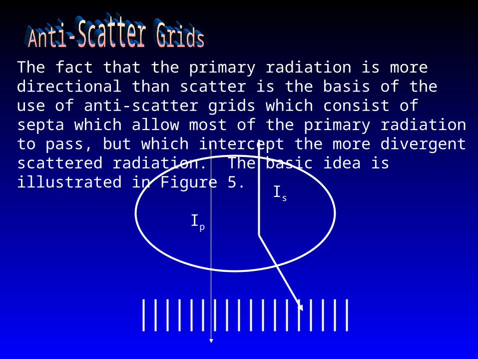
The fact that the primary radiation is more directional than scatter is the basis of the use of anti-scatter grids which consist of septa which allow most of the primary radiation to pass, but which intercept the more divergent scattered radiation. The basic idea is illustrated in Figure 5.

Ip

Is

The grid shown in Figure 4 is called a parallel grid and usually consists of numbers in the range of 100 septa per inch made of lead or tantalum.

The advantage of a parallel grid is that it is easily positioned.

A disadvantage is that for large fields of view, the primary transmission decreases at the edges of the field of view where the primary radiation enters the grid at appreciable angle leading to “grid cutoff”.

Other options include focused grids in which the grid septa are focused toward the x-ray source and crossed grids with septa going in each direction. These are shown in Figure 6.

Focused grids have improved transmission of primary radiation but must be carefully aligned. Obviously, putting a focused grid in upside down would result in very poor transmission. The crossed grid provides the lowest resultant scatter fractions, but provides reduced primary transmission.

The factor by which the mAs must be increased to achieve the same detector exposure following the reduction of scatter and, to a lesser extent, primary radiation is called the Bucky factor.

This has nothing to do with the University of Wisconsin mascot but is derived from the name of the inventor of the grid.

An important parameter characterizing a grid is the grid ratio Rg defined as the ratio of the septal length to the septal spacing. Figure 7 shows the typical transmission Ts for scattered radiation as a function of grid ratio.

Most of the scatter reduction is achieved at the lower grid ratios. Further reduction comes at the expense of increased Bucky factor.

Air gaps are sometimes used instead of grids. The extra distance between the patient and detector allows the more divergent scattered radiation to miss the detector.

Since air gaps and grids eliminate some of the same radiation, the effects of simultaneous use of air gaps and grids are not multiplicative.

The use of an air gap increases magnification which can either increase or decrease spatial resolution depending upon whether resolution is limited by focal spot blurring or the detector.

The effectiveness of a grid depends on the details of the imaging situation.

In general when there is a large scatter fraction present, it makes sense to use a grid. For small scatter fractions, the decrease in primary transmission might be too large a detriment. The grids physical transmission properties are described by the selectivity which is defined in terms of the primary tranmission Tp and the scatter transmission Ts as

(10)

The grid produces the following intensity transformations,

(11)

Rewriting the scatter fraction in terms of the scatter to primary ratio using equations 2 and 3, we can calculate the new scatter fraction with the grid in place. Without the grid we have,

(12)

With the grid the scatter fraction becomes,

(13)

Figure 8 shows the improvement in scatter fraction FG achieved with grids of various selectivities for various scatter fractions F.

For =10, F=0.8 which gives R =4, we get FG of about 0.3.

The contrast after insertion of a grid CG is related to the contrast in the presence of scatter

by the (note missing words in text)

contrast improvement factor KG defined as

(14)

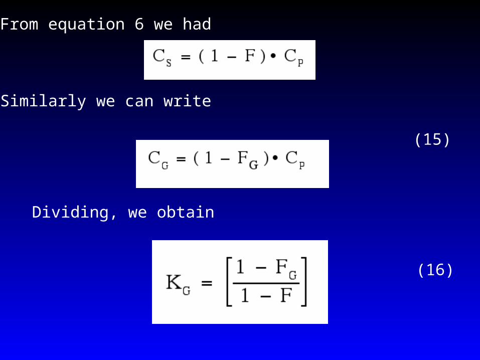
From equation 6 we had

Similarly we can write

(15)

Dividing, we obtain

(16)

Plugging in for FG from equation 13

and doing a little algebra, we obtain,

(17)

The selectivity is a more fundamental property of the grid than KG which, as can be seen from equation 17, is highly dependent on the scatter to primary ratio.

The dependence of KG on is shown in Figure 8 for three values of R.

(13)

The dependence of KG on is shown in Figure 8 for three values of R.

QUESTION--Can insertion of a grid reduce the required exposure?

Since contrast is improved and required exposure depends on contrast we might expect that under certain circumstances, the use of a grid might reduce exposure requirements. First we will consider the case of an ideal grid with perfect scatter rejection and complete primary transmission. Then we will consider the case of a real grid. We will consider a mono-energetic x-ray beam so that we can easily calculate the quantum noise.

Suppose with no scatter present it is possible to see an object of contrast Cp. We previously derived the fact that the required detected fluence Np for a given SNR, object area A and primary subject transmission is given by

(18)

Recall that in this equation s is understood to be the differential signal due to the attenuation of the low contrast object as opposed to S, the total signal detected.

In the case where scatter is detected and the contrast is reduced in accordance with equation 6, the new required exposure, including the detected scatter N’s is

(19)

where

(20)

and is the factor by which the exposure must be increased in order to compensate for the increased scatter fraction.

A common mistake (made in one of my own early publications) is to argue that since the required exposure is increased by a factor of 1 / (1-F ) 2 , the mAs must be increased by this factor in order to see the object, and therefore, the insertion of a grid would reduce exposure by a factor of 1 / (1-F ) 2.

However, this argument ignores the fact that, whereas only primary radiation was used to satisfy the exposure requirement in the case with no scatter, when scatter is present it contributes to the detected exposure and alters the fractional quantum fluctuations. Lets look at this more carefully.

From F = Ns / ( Np + Ns) we get

(21)

Using equation 20 and the fact that scatter fraction is not altered by the mAs increase we get

(22)

But since from equations 18 and 19

(23)

It follows that

(24)

Therefore, by eliminating the need to increase the mAs by a factor of , the use of an ideal grid reduces the required exposure by a factor of 1 / (1-F) rather than 1 / (1-F) 2.

Another way of calculating this result is to consider absolute signal and quantum noise amplitudes rather than contrast. In that case, scatter does not change the differential signal, (the attenuation by the low contrast object) but it does increase the absolute size of the noise since the square root of the total detected fluence increases. Let’s try this.

For the case of no scatter the differential signal to noise ratio is given by

(25)

With scatter and mAs increased by a factor of

(26)

The object will be detected equally well provided that the signal to noise ratio is the same. Therefore we can equate the two expressions in equations 25 and 26 to obtain = 1/(1-F) as above.

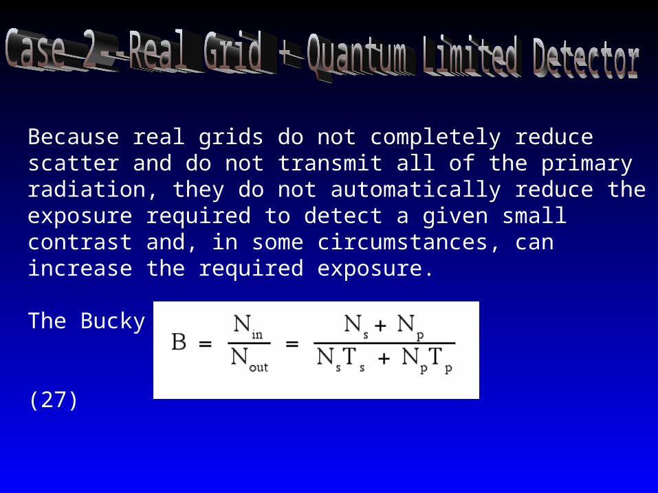
Because real grids do not completely reduce scatter and do not transmit all of the primary radiation, they do not automatically reduce the exposure required to detect a given small contrast and, in some circumstances, can increase the required exposure.

The Bucky factor B is given by

(27)

Where in and out refer to the grid and Ts and Tp are the grid transmissions for scatter and primary respectively.

For systems such as film which generally require a narrow range of exposure to remain in the linear range, exposure must be increased by the Bucky factor just to satisfy exposure conditions.

For systems such as phosphor plates and image intensifiers which can approach quantum limited systems in certain circumstances we can apply our previous analysis to determine the factor by which exposure must be altered to provide equivalent low contrast object detection.

Assume that in the presence of scatter a contrast Cs is just seen with exposure Np +Ns, we can write

(28) Cs2 AT

=

With the grid inserted and the exposure modified by a factor of , recalling that CG = CsKG, we get the following expression after the grid,

(29)

For the signal to noise ratio to be the same in each case we must have

(30)

or

(31)

For B< (KG)2, exposure is reduced by using the grid. When small amounts of scatter are present, KG is small ( see Figure 8) and will be greater than 1.

Several alternate approaches to scatter reduction have been implemented. These usually involved some sort of scanning procedure which limits the extent of the x-ray beam to a scanning point or line. A generic example of a line scan system is shown in Figure10.

Due to the coordinated motion of the slit pairs, most of the scattered radiation is removed. These systems have been shown to provide greatly improved contrast in applications such as chest radiography. Their main drawback is that exposure times are increased by the ratio of the field of view to the slit width and tube loading becomes a serious problem.

Commercial systems using line scan geometries have been introduced in connection with a process called exposure equalization in which detected signal feedback schemes permit alteration of the exposure on a line by line basis in order to reduce the dynamic range of information contained in the image. This results in improved SNR in the poorly transmissive regions of the image. Because the highly transmissive areas are reduced in intensity, their contribution to the scatter fraction in nearby, less transmissive areas is reduced. The result is that low contrast objects such as lung tumors can be detected more easily.

Other manufacturers have used point scanned systems which remove essentially all effects of scatter. These systems had extremely high tube loading and were generally limited to pediatric patients.

There are several applications where it is advantageous to estimate the amount of scatter present in order to perform quantitative image processing. Examples of this include dual energy imaging for determination of bone mineral, dual energy chest imaging, where images of differing energies are used to remove bone or soft tissue, and dual energy DSA where it is desired to remove the effects of soft tissue misregistration.

One technique is to simply place an array of small lead absorbers in the image and take an extra exposure in which the signal behind the absorbers can be used to estimate the local amount of scatter.

Since the finite size of the absorbers perturbs the scatter field to some extent, such measurements are usually tried on phantoms using absorbers of decreasing size and then extrapolating to the scatter value which would be obtained with absorbers of zero radius.

Another calculational approach is to use a point spread function method which assumes that, associated with every point in the detected primary radiation field, there is a well defined distribution of scattered radiation as shown in Figure 11.

For a single primary transmission ray at the point x,y there is an associated amount of scatter P(x-x’,y-y’) at point x’,y’. This function is called the scatter point spread function and can be used to estimate the scatter image if the primary image is known.

This is described by equation 32.

(32)

There are two difficulties with trying to calculate a scatter image by this method

1 The primary intensity is not available since it is Ip + Is that is measured.

2 The point spread function depends on thickness.

A first approximation to the scatter image is to blur the detected image and pretend that the detected image is the primary image.

This works well if the scatter fraction is small, provided that the right amount of blurring is used.

More accurate methods such as those used by Naimuddin and Molloi attempt to establish a relationship between the detected image intensity and the scatter fraction.

This makes use of the knowledge that scatter fractions are typically higher in the regions of decreasing transmission.

Typically a chest phantom with lead blockers is used to get a graph of scatter fraction versus detected intensity as shown schematically in Figure 12.

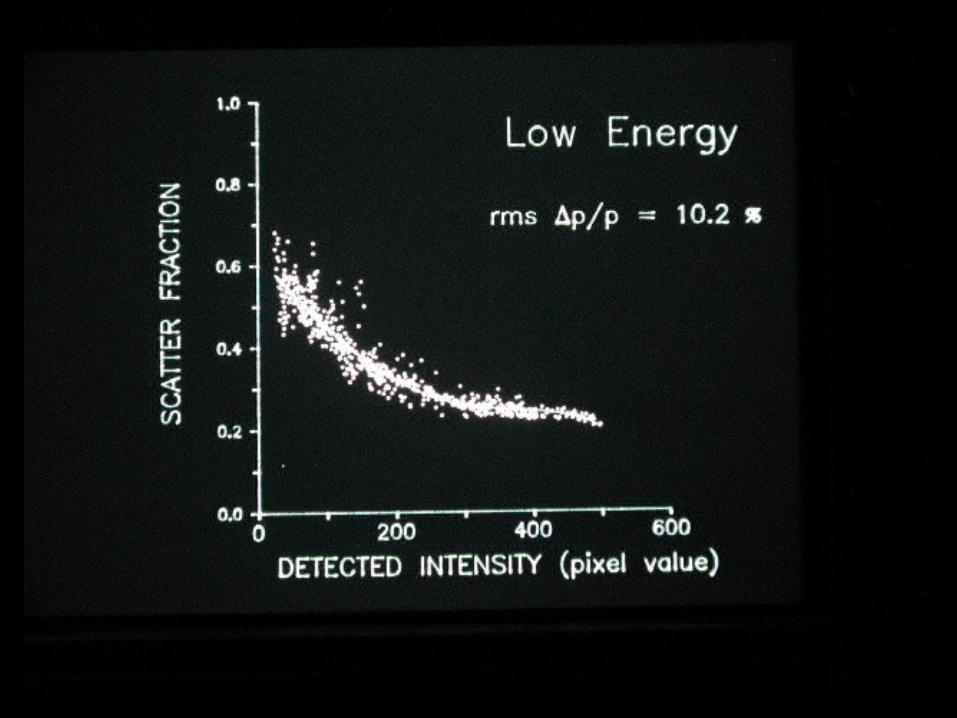
The spread in data points around the fitted curve reflects the fact that detected intensity alone is not an absolute predictor of scatter fraction.

Scatter fraction also depends on the configuration of scattering material in adjacent regions. Nevertheless, the variations from a polynomial fit to the chest phantom data are not excessively large in the chest.

When corrections for patient thickness and beam energy are made, scatter fraction and therefore the scatter image can be estimated fairly reliably.

Separate polynomial estimators are required for different imaging sites in the body.

The scatter correction scheme of Molloi is shown in Figure 13. Note that before the scatter image is subtracted from the detected image to produce a scatter free estimate it is blurred to remove detail not physically present in the actual scatter image.

The use of such a scheme to estimate the scatter image is shown in Figure 14 for the case of chest radiography.

Note that the scatter image is essentially a blurred version of the original image containing only low spatial frequencies.

Capillary Optics

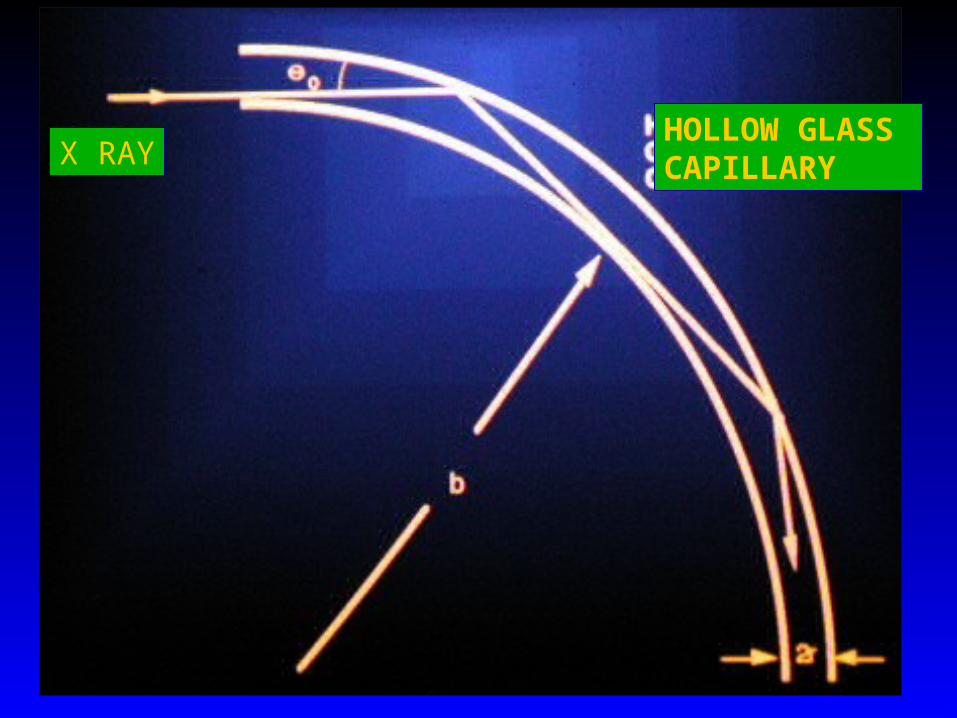
HOLLOW GLASS CAPILLARYX RAY

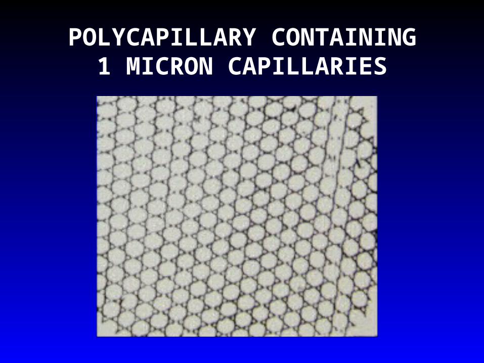
POLYCAPILLARY CONTAINING1 MICRON CAPILLARIES

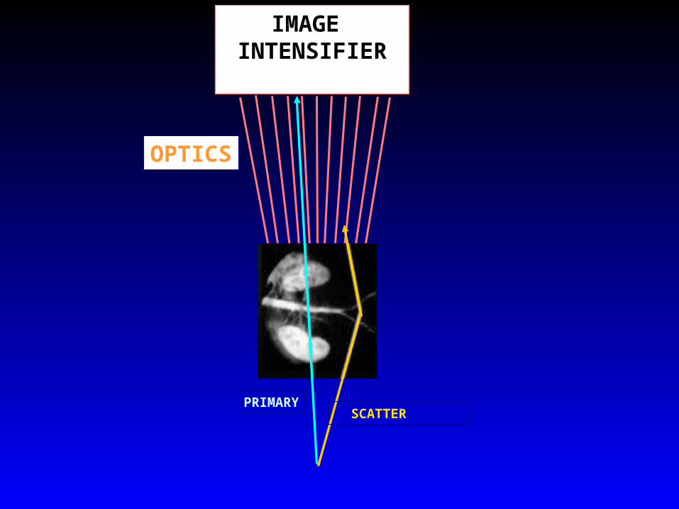
IMAGE INTENSIFIER

OPTICS

PRIMARY SCATTER

PATIENT EXIT BLUR

NORMAL MAGNIFICATIONBLUR

REDUCEDBLUR DUETO OPTICS

PATIENT

EXTENDED FOCAL SPOT