occupational structure and the sources of income ... · arthur sakamoto department of sociology –...
TRANSCRIPT

1
Occupational structure and the sources of income inequality: a comparison between Brazil and the U.S.
Alexandre Gori Maia
Instituto de Economia – Universidade Estadual de Campinas (IE/UNICAMP)
Email: [email protected]
Arthur Sakamoto
Department of Sociology – Texas A&M University
Email: [email protected]
Área 13 – Economia do Trabalho
Abstract: Characterized by a lower level of economic development than the U.S., the Brazilian labor force
has lower levels of education, wages, and occupational skill. While both countries have high levels of
inequality, low economic development in Brazil reduces the proportion of total income that accrues to the
bottom two quintiles of the income distribution. In recent decades, inequality has declined in Brazil by
increasing income cash transfer programs while reducing the proportion of the labor force employed in the
lowest skilled occupations. However, this trend has been somewhat offset by the concurrent increase in
professional and other upper white-collar occupations. By contrast, in the U.S., where cash transfer programs
have not increased, inequality rose over this time period largely due to higher earnings accruing to the top
decile of households. This rise in inequality in the U.S. appears to be less immediately associated with
occupational structure in general but somewhat more immediately connected with rising earnings and earnings
inequality among high skill professionals. Our analysis thus suggests that occupational structure has more
general effects on income inequality at a lower level of economic development. At a higher level of
development, inequality seems to increase in large part due to rising inequality among high skill employees
which may be more related to unobserved variables within occupations.
Keywords: labor market; inequality decomposition; middle class; top income; labor structure
Resumo: Caracterizada por um baixo nível de desenvolvimento econômico em comparação aos EUA, a força
de trabalho brasileira possui baixos níveis de educação, salários e habilidades ocupacionais. Embora os dois
países apresentem altos níveis de desigualdade, o baixo desenvolvimento econômico no Brasil seria um dos
responsáveis pela baixa proporção do rendimento total acumulado pelos dois últimos quintos da distribuição
de renda. Nas últimas décadas, a desigualdade diminuiu no Brasil, tanto pela expansão dos programas de
transferência de renda, quanto pela redução da proporção da força de trabalho empregada em ocupações de
baixa qualificação. Por outro lado, nos EUA, onde não houve mudanças substanciais nos programas de
transferência de renda, a desigualdade aumentou sobretudo devido ao expressivo crescimento da renda das
famílias dos décimos superiores da distribuição de renda. Este crescrimento da desigualdade nos EUA parece
menos associado à composição da estrutura ocupacional, mas ao crescimento da desigualdade dentro do grupo
de profissionais mais qualificados. As análises sugerem, assim, que mudanças na estrutura ocupacional teria
efeitos mais imediatos na desigualdade de renda em um nível inferior de desenvolvimento econômico. Em
estágios mais elevados, a desigualdade parece aumentar, em grande parte, devido à crescente desigualdade
entre os profissionais altamente qualificados, que estaria relacionada a fatores não observáveis dentro das
ocupações.
Palavras-chave: mercado de trabalho; decomposição da desigualdade; classe média; distribuição de renda;
estrutura ocupacional
JEL: J21; J31; J82

2
Introduction
Occupations are central to the stratification systems of industrial countries, but they have played little
role in empirical attempts to explain the well-documented dynamics of income inequality. The occupational
structure reflects the organization of the production and the level of technological development, and will affects
the demand for different types of products and services, as well as the demand and supply for different types
of labor (Blau & Duncan, 1967; Banerjee & Newman, 1993). Occupations also tend to define in a large extent
the current and future perspective of income generation, playing a central role to explain social relations,
economic opportunities and inequalities between individuals in modern societies (Goldthorpe, 2000; Rose &
Harrison, 2007).
Brazil and the U.S. provide an interesting comparison to understand the impacts of occupational
structure on socioeconomic inequalities. They are the two biggest economies and populations of America and
shared important peculiarities in their process of socioeconomic development. These countries were colonized
almost simultaneously, based initially in the agricultural production in big farmers with slave labor, and
witnessed singular trajectories of social, economic and institutional development (Acemoglu & Robinson,
2012; Furtado, 1986). Nowadays, they present high levels of socioeconomic inequality and also huge
differences in their levels of socioeconomic development.
Differences in the structure of their labor markets would explain in large extent their current levels of
socioeconomic development and inequalities. Labor productivity in substantially lower in Brazil for all
economic activities, determining levels of labor remuneration substantially lower in comparison with the U.S.,
as well as the low participation of skilled labors in its occupational structure (Maia & Menezes, 2014). The
oversupply of unskilled workers and the few opportunities of social mobility have determined an occupational
structure with high levels of segmentation and inequality (Ulyssea, 2006). Nowadays, the concentration of
unskilled occupations in the Brazilian labor structure and its extreme pay differences in relation to the small
number of skilled occupations contribute in large extent to explain the high levels of inequality in the labor
market (Maia, 2013).
Economic growth, that would be essential to generate new opportunities of employment and social
mobility (Piketty, 2014), have not been able to improve consistently the process of social mobility in this
country, which is still characterized by high levels of inequality of opportunities (Bourguignon, et al., 2007;
Ribeiro, 2012). Despite some recent improvements, the quality of education, which plays a central role
improving human and social capital, is still very low in Brazil and would help to explain the low development
of its occupational structure as well, as the restrict process of social mobility (Ferreira, et al., 2011). Huge
differences in the level of regional development have also been pointed as an important determinant of
socioeconomic inequalities in Brazil (Neto, 1997), as well as the extreme conditions of life and access to basic
infrastructure that some social groups are submitted to (Pinheiro, et al., 2009).
In turn, the American occupational structure would reflect an economy more specialized in services of
high productivity. Influenced by the emergence of new information and communications technologies, this
country witnessed in the last decades a substantial rise of managerial and professional occupations, over the
reduction of agricultural and manufacturing jobs, characterizing the so called informational society (Aoyama
& Castells, 2002). Earning inequalities is also high, but mainly characterized by intra-occupational differences,
suggesting a lower level of occupational segmentation in their labor market (Kim & Sakamoto, 2008).
Nonetheless, the U.S. recently observed a substantial increase in the demand for high skills jobs and in
the earnings differentials between those workers with and without college diploma. Acemoglu & Autor (2010)
suggest that the returns to skills (and to education) is determined by a race between the increase in the demand
for skills in the labor market and the supply of qualified workers, notably workers with college diploma. Since
the demand grew faster than supply in some especific high skilled occupations, earnings grew faster for
qualified workers, as well as the inequality between the groups of educational attainment. Autor et al. (2003)
also highlight a process of polarization in the American occupational structure, this means, reduction of
medium skill occupations and increase of top and bottom occupational groups. Medium occupational groups
are characterized by routine tasks that can be easily substituted by machines following explicit programmed

3
rules. In turn, top and bottom occupations are characterized by tasks that demand problem solving, judgment,
and creativity in the former, and flexibility and physical adaptability in the latter. Activities that can not be
easily specified as a series of instructions and much less susceptible to an automation process.
Overall, there are several aspects of social inequality in Brazil and in the U.S. that are strictly related
to the structure of their labor market. This study highlights how the process of economic development and
changes in the occupational structure contribute to explain the levels of income and earnings inequality. More
specifically, it explores the dynamics of inequality between 1983 and 2013, highlighting: i) how low level of
economic development and the concentration of bottom low skilled occupations in Brazil reduces the
proportion of total income that accrues to the bottom deciles of the income distribution; ii) how the rise of
wages within the most qualified professional occupations in the U.S. have contributed to increase inequality.
Finally, the study discusses the effects of the occupational structure on income inequality at different levels of
economic development.
Material and methods
Data base
Analyses are based on pooled annual data from the Brazilian Pesquisa Nacional por Amostra de
Domicílios (PNAD), sponsored by the IBGE (Instituto Brasileiro de Geografia e Estatística), and the
American Current Population Survey (CPS), sponsored jointly by the U.S. BLS (Bureau of Labor Statistics)
and the U.S. Census Bureau. The period of analyses comprehend the years between 1983 and 2013. PNAD is
a household sample collected annually1 and is nationally representative of Brazilian territory (with the slight
exception of a few remote rural areas in six northern states which represented less than 3% of Brazilian
population in 2000 [IBGE 1995])2. In turn, CPS is a household sample survey applied monthly in the U.S.
(BLS 2000) and we used data of its Annual Social and Economic Supplement (ASEC).
Monetary values in PNAD refers to self-reported monthly values usually received in the reference year.
Self-reported annual income and earnings in CPS were divided by 12 to be comparable with the Brazilian
monthly values. Nominal values were deflated to July 2013 using the INPC (Índice Nacional de Preços ao
Consumidor) in Brazil and the CPI (Consumer Price Index) in the U.S.. Subsequently, Brazilian earnings were
converted to International PPP (Purchasing Parity Power) dollars using the exchange rate available at World
Data Bank3. PPP are both currency converters and spatial price deflators that equalize the purchasing power
of different currencies in the process of conversion (International Comparison Programa, 2011).
In both countries, top values were censored at the 1% level in order to consider methodological changes
implement in the methodology of top-coding applied by the CPS4. In other words, values exceeding the top-
code threshold (99-th percentile) were simply recoded with the threshold. This procedure were implement
independently to individual earnings and household per capita income. This technique prizes by the simplicity
and robustness to changes implemented in the top-code methodology, without further assumptions about the
probability distribution of the income variables5.
1 Between 1983 and 2011, PNAD was not applied in the years 1991, 1994, 2000, and 2010. 2 PNAD excludes the rural areas of the states of Rondônia, Acre, Amazonas, Roraima, Pará and Amapá. Since 2004, these areas
have been added to the PNAD sampling frame, but for our purposes of maintaining historical comparibility, those areas were not
considered in this study. 3 In July 1st 2013, the exchange rate was 1.81 Brazilian Reais for each 1 PPP international dollar (World Bank, 2015). 4 Between 1962 and 1995, the values exceeding the top-code threshold in CPS were simply recoded with the threshold. Between
1996 and 2010, the Census Bureau introduced replacement values to take the place of top-coded values, depending on characteristics
such as race, gender, and full time status. Since 2011, all incomes above the top-code are rounded to two significant digits and then
exchanged among individuals within a bounded interval (Minnesota Population Center, 2015). 5 See, for example, Piketty & Saez, 2003).

4
We considered as employed those who were 16 years or older and, during the reference week (a) did
any work at all (for at least 1 hour) as a paid employee; worked in his own businesses, profession, or on his
own farm; or (b) were not working, but who had a job or business from which he was temporarily absent.
Persons whose job was Armed Forces and those with non-positive earnings were not considered in both the
surveys.
Occupational Structure
We developed a typology of occupational stratification to analyze the levels of earnings inequality in
the Brazilian and American labor markets. Occupation codes provided by PNAD and CPS were classified into
common occupational groups in Brazil and in the U.S. The classification was based on skills, education,
training, credentials and also social prestige or power. Since these concepts are very similar to those used by
the Brazilian CBO (Classificação Brasileira de Ocupações) and the American OCS (Occupational
Classification System), the groups reflect mainly the structure proposed by these systems (BLS, 2000; CBO,
2010). As a result, occupational codes of PNAD and CPS were initially aggregated into 20 occupational groups
(see Table 1). According to the analytical convenience, these 20 two-digit occupational groups can also be
aggregated into 6 one-digit occupational groups: 1) Managers; 2) Professionals; 3) Specialists; 4) Sales and
Laborers; 5) Low Services; 6) Farming.
Table 1 – One-digit and two-digit occupational groups
One-Digit
Occupational
Group
Two-Digits
Occupational Group
Description
Management occupations Chiefs, managers, first-line supervisors
Professionals Legal Occupations Lawyers, judges, legal assistants, and related
Biological and Health Agricultural, biological, health and related scientists
Maths and related Computer, mathematics, engineering and related scientists
Social/Human Sciences Financial specialists, Social Scientists, Social Services and related occ.
Education and Library Teachers, instructors, librarians and related
Specialists Entertainment/Related Arts, Design, Entertainment, Sports, and Media occupations
Technicians Technologists and technicians of several areas
Clerks Office clerks, secretaries, administrative assistants and related
Protective services Fire fighters, police, criminal investigators, and related
Customer service Customer service representatives, receptionists, and related
Sales and
Laborers
Sales Retail sales, cashiers, representatives and related sales agents
Installation and Repair Installation, maintenance, and repair workers
Construction/Extraction Masons, carpenters, painters, extraction workers and related occ.
Production Assemblers, fabricators, operators and related production workers
Transportation/Moving Bus/truck drivers, and related laborers in transport and material moving
Low Services Personal care/Others Hairdressers, personal care aides and related workers
Food and serving Cooks, waiters, food preparation and related
Building and cleaning Housekeeping cleaners, janitors, and related
Farming Occupations Farming, fishing and forestry occupations
The hierarchy of the occupational groups were mainly based on the level of skills, qualification,
earnings and also social and political power to control the capital or the labor. For example, managers do not
have necessary higher levels of education than professionals, but they tend to possess the power to control

5
large number of employees in public and private companies. Professionals are highly skilled workers, usually
with superior diploma, who also tend to receive high earnings. Specialists are workers with intermediate levels
of education and earnings, although many positions require a superior or a technical diploma. Sales and
laborers present low level of education and earnings, usually with no more than secondary education. They
are one step above the low services workers, the non-agricultural occupations with the lowest levels of
qualification and remuneration. Finally, faming workers perform manual and low-paid activities in agriculture,
fishing or forestry.
Decomposing the variation in the per capita income inequality
We first used the Gini index to analyze inequality in the distribution of per capita income. Gini index
(0 G < 1) is based on a concentration curve (Lorenz curve), representing the relation between the accumulated
concentration of the population (X-axis) and the accumulated concentration of income (Y-axis). The area
between the Lorenz curve and the X-axis is represented by 𝛽, and is reference to compute the Gini index:
𝐺 = 1 − 2𝛽 (1)
Since the per capita income can be composed by different sources, we can also decompose the Gini
index to consider the contribution of each source to total inequality. For this specific purpose, the Gini index
can be represented by the weighted sum of concentration ratios (𝐶𝑠) observed for each source of income f.
More specifically (Hoffmann, 2006):
𝐺 = ∑ 𝑝𝑠𝐶𝑠𝑘𝑠=1 (2)
Where 𝑝𝑠 is the total share of the s-th source of income, and 𝐶𝑠 is its respective concentration ratio,
which can be given by:
𝐶𝑠 = 1 − 2𝛽𝑠 (3)
Similarly to the Gini index, the concentration ratio (1<𝐶𝑠<1) is based on a specific concentration curve
for each source of income. The difference is that the accumulated concentration of income (Y-axis) now
represents the accumulated concentration of the s-th source of income, holding the same hierarchy of the per
capita incomes. Thus, 𝛽𝑠 represents the area between the s-th concentration curve and the X-axis.
Using expression (3) we can evaluate, for example, in what extent total inequality is due to income
from labor and other sources. We can also represent the variation in the Gini index between two periods (∆𝐺)
as a function of: i) changes in the composition of the sources of income; ii) changes in the concentration ratios
of the sources of income. Making some algebraic transformations, the variation in the Gini index will be given
by (Hoffmann, 2006):
∆𝐺 = ∑ [(𝐶�̅� − �̅�)∆𝑝𝑠⏟ 𝑐𝑜𝑚𝑝𝑜𝑠𝑖𝑡𝑖𝑜𝑛
+ �̅�𝑠∆𝐶𝑠⏟ 𝑖𝑛𝑒𝑞𝑢𝑎𝑙𝑖𝑡𝑦
]𝑘𝑠=1 (4)
Where 𝐶�̅�, �̅� e �̅�𝑠 represent the average values for the respective measures in the two periods. The first
term represent the composition effect, this means, the share of the variation in the Gini index that is due to
changes in the proportion of income accumulated by each source. The second term represent the inequality
effect, this means, the share of the variation that is due to changes in the concentration ratio of each source of
income.
Decomposing the variation in the individual earnings inequality
Specific analyses for individual earnings inequality in the labor market were done using Theil indicator.
Suppose Yi the i-th individual earnings and Y the total earnings in a population of size n. Theil (0 T ln n)
will be given by (Hoffmann, 1998):

6
𝑇 = ∑𝑌𝑖
𝑌ln 𝑛
𝑌𝑖
𝑌
𝑛𝑖=1 (6)
Both Theil and Gini index satisfy the Pigou-Dalton condition, this means, they will increase in value
for regressive transfers of income. In addition, Theil is relatively insensitive to changes occurred in the bottom,
middle or upper bound of the income distribution (Hoffmann, 1992). Gini is relatively more sensitive to
changes in intervals with higher density of frequency, usually in the middle of the income distribution.
A main advantage of the Theil indicator is that it can be linearly decomposed into two main
components: i) differences between groups; ii) differences within groups. Suppose, for example, an employed
population divided into g occupational groups. The total earnings inequality can be represented by the sum of
the inequality due to earnings differences between the occupational groups (B) and earnings differences within
the occupational groups (W). B and W will be given by (Hoffmann, 1998):
𝑇 = 𝐵 +𝑊 (7)
𝐵 = ∑𝑌𝑗
𝑌ln𝑌𝑗 𝑌⁄
𝑛𝑗 𝑛⁄
𝑔𝑗=1 = ∑ 𝑝𝑗ln
𝑝𝑗
𝑛𝑗 𝑛⁄
𝑔𝑗=1 = ∑ 𝑝𝑗 𝐵𝑗
𝑔𝑗=1 (8)
𝑊 = ∑ 𝑝𝑗𝑊𝑗𝑔𝑗=1 (9)
Where 𝑌𝑗 is the total earnings accumulated by the j-th occupational group, 𝑝𝑗 is the respective share of
the total earnings, 𝑛𝑗 is the respective population, and 𝐵𝑗 is the between inequality component for the j-th
occupational group. 𝑊𝑗 is the inequality within the j-th occupational group and is computed similarly to
expression (6), restricting analysis to the population of the j-th occupational group.
We can also evaluate in what extent variation in the Theil indicator in a period (∆𝑇) was due to: i)
changes in the differences between the groups of analysis (∆𝐵); ii) changes in the differences within the groups
(∆𝑊). More specifically, we will have:
𝑇 = ∆𝐵 + ∆𝑊 (10)
∆𝑇 = ∑ [∆(𝑝𝑗 𝐵𝑗)⏟ 𝑏𝑒𝑡𝑤𝑒𝑒𝑛
+ ∆(𝑝𝑗𝑊𝑗)⏟ 𝑤𝑖𝑡ℎ𝑖𝑛
]𝑔𝑗=1 (11)
The first term in expression (11) represents the share of the variation in the Theil indicator due to
changes in the between component of the j-th group. Groups can contribute to modify between inequality
through changes in their participation in the occupational structure (∆𝑝𝑗) or changes in their relative
accumulation of earnings (∆𝐵𝑗). The second term represents the contribution of changes in the within
component of the j-th group. Similarly, groups can modify within inequality through changes in their
participation (∆𝑝𝑗) or changes in the patterns of inequality within these group (∆𝑊𝑗). Expressions (8) through (9) can also be developed to consider additional levels of disaggregation.
Suppose, for example, that, in addition to g occupational groups, population is also divided into d groups of
education. B and W indicators of inequality for two levels of disaggregation can be given by:
𝐵2 = ∑ ∑ 𝑝𝑗𝑙 𝐵𝑗𝑙𝑑𝑙=1
𝑔𝑗=1 (12)
𝑊2 = ∑ ∑ 𝑝𝑗𝑙𝑊𝑗𝑙𝑑𝑙=1
𝑔𝑗=1 (13)
Now B2 represents the share of total inequality due to the differences between all the combinations of
the two groups of analysis, occupations and education, as well as W2 represents the share due to the differences
within these combinations of groups. The higher the value of B2, the higher the explanatory power of these
groups of analysis over the total accumulation of income.
The marginal contribution of a variable represents the share of the total between inequality that can
only be explained by its respective group of categories. It can be easily computed comparing two measures of
between inequality: i) considering all groups of analysis (unrestricted B); ii) excluding the groups of interest
(restricted B). For example, the marginal contribution of the d categories of education (𝐵𝑑) will be given by:

7
𝛽𝑑 = ∑ ∑ 𝑝𝑗𝑙 𝐵𝑗𝑙𝑑𝑙=1
𝑔𝑗=1⏟ 𝑢𝑛𝑟𝑒𝑠𝑡𝑟𝑖𝑐𝑡𝑒𝑑
− ∑ 𝑝𝑗 𝐵𝑗𝑔𝑗=1⏟ 𝑟𝑒𝑠𝑡𝑟𝑖𝑐𝑡𝑒𝑑
(14)
Equations (12) to (14) can also be easily extended to consider k levels of analysis. In this study, 6 levels
of analysis are considered: i) occupation (20 two-digit occupational groups); ii) education (no diploma, no
more than elementary diploma; no more than secondary diploma; college diploma or more); iii) age (16-19;
20-29; 30-39; 40-49; 50;59; 60 or more); iv) gender (male and female); v) race (white, black and others); and
vi) region (in Brazil: North, Northeast, Southeast, South and Midwest; in the US: West, Northeast, Southeast,
Southwest, Midwest).
The contribution of labor income to total inequality
Brazil and the U.S. were jointly responsible for more than 500 million people living in the same
America in 2013 (Table 2), which were submitted to extreme levels of socioeconomic inequality. Changes in
the socioeconomic structure in the last 30 years were more pronounced in Brazil. For example, population
grew 60% in Brazil between 1983 and 2013, and just 36% in the U.S.. As remarkable as the population growth
in Brazil was the sharp reduction in its number of member per household (31%, from 4.4 in 1983 to 3.1 in
2013), mainly children under 16, a main consequence of the fast decline in the fertility rate in the 80s and 90s
(Maia & Sakamoto, 2014)6. As a result of both demographic changes and economic dynamics, per capita
income grew faster and unusually in Brazil, reducing the huge differences in relation to the U.S.. In 2013,
Brazil had 197 million of people living with a per capita income of 561 dollars per month, 60% higher than in
1992 (274 dollars per month), but still 4.1 times lower than in the U.S. (2,279 dollars per month).
Table 2 - Demographic and inequality indicators – Brazil and the U.S., 1983 and 2013
Indicator Brazil US
1983 2013 1983 2013
N (1,000s) 123,393 197,497 229,587 311,116
N/household 4.4 3.1 2.7 2.5
Per capita income 274 561 1,747 2,279
Percentile
40 110 292 1,157 1,344
50 144 371 1,404 1,686
90 647 1,174 3,478 4,731
99 2,206 4,201 7,317 12,118
% Share of total income
40% Poorest 9.0 11.6 14.5 12.8
50% 47.6 49.9 57.1 55.6
9% 35.3 31.0 24.1 26.3
1% Richest 8.0 7.5 4.3 5.3
Gini (%) 56.4 50.1 40.0 45.0 Source: PNAD (IBGE) and CPS (BLS).
6 Between 1983 and 2012, fertility rate dropped from 3.7 to 1.8 births per woman in Brazil. In the U.S., a tenuous increase, from 1.8
to 1.9.

8
In addition to huge differences between the average incomes, the gap between the levels of inequality
within these countries is also substantial. Although both countries are characterized by singular levels of
inequality, they are particularly high in Brazil. In this country, the share of the total income accumulated by
the 40% poorest are comparable to the share accumulated by the 1% richest, even considering the censoring
at the per capita income of the 1% richest, which tend naturally to underestimate real inequality. When
considering the income accumulated by the 10% richest (the sum of the 1% censored highest values and the
income of the next 9% richest), it was 3.3 times higher than the share accumulated by the Brazilian 40% poorest
in 2013. Differences are less extreme in the U.S., where the ratio between the share of income accumulated by
the 10% richest and the 40% poorest was 2.5 in 2013 and the Gini index was 5 percentage points lower than
in Brazil.
A main responsible for the higher levels of inequality in Brazil is the extreme concentration of people
in the lower bound of the income distribution. Even the 50% middle group of the income distribution in Brazil
presents very low levels of per capita incomes in comparison to their American counterparts, and, thus, they
do not accumulate a substantial share of the total income (50% in Brazil and 56% in the U.S. in 2013). As a
result, differences between the lowest and middle percentiles in Brazil and in the U.S. are higher than
differences between the highest percentiles. For example, in 2013 the percentile 40 in the U.S. was 4.6 times
higher than in Brazil, meanwhile the percentile 90 was 4.0 times higher and the percentile 99 was just 2.9 times
higher. The scenario in 1983 was more dramatic, when the percentile 40 in the U.S. was 10.5 times higher than
in Brazil and the percentile 90 was 5.4 higher.
The reduction in the levels of differences between Brazil and the U.S. is a result of opposite trends
witnessed in the dynamics of inequality in this period (Figure 1). Inequality reduced sharply in Brazil,
especially in the 2000s. For example, Gini index fell 9 percentage points between 2001 and 2013, and the ratio
between the share of the total income accumulated by the 10% richest and the 40% poorest reduced from 5.5
to 4.0. Meanwhile, in a continuous growth of the income inequality in the U.S., Gini index increased 5
percentage points between 1983 and 2013, and the ratio between the share of the total income accumulated by
the 10% richest and the 40% poorest increased from 3.0 to 3.5.
Figure 1 - Gini index and the ratio between the percentile 90 and the percentile 40 of the per capita income.
Brazil and the U.S., 1983 to 2013 Brazil
US
Source: PNAD (IBGE) and CPS (BLS).
These divergent trends reproduces, in large extent, particular dynamics of labor incomes observed in
each country. Figure 2 presents the accumulated variation in the per capita income (index, 1983=100) of the
10% richest and the 40% poorest, disaggregated into two main sources of income: labor and others (pension,
investments, rents, social benefits, cash transfer programs, among others). The trends highlights how labor
income grew faster for the poorest in Brazil and faster for the richest in the U.S.. Between 1983 and 2013
average per capita income from labor (labor income) more than doubled for the 40% poorest (grew 107%) and

9
grew just 67% for the 10% richest in Brazil. Divergent trends were witnessed in the U.S., where labor income
grew 69% for the 10% richest and remained mostly unchanged for the 40% poorest (grew just 9%).
Figure 2 - Accumulated variation (index, 1983=100) in the average per capita income from labor and other
sources for the 10% richest and 40% poorest – Brazil and the U.S., 1983 to 2013 Brazil
US
Source: PNAD (IBGE) and CPS (BLS).
The accumulated variation in the average income from other sources of the 40% poorest in Brazil is
represented by a secondary vertical axis (in red), in order to stress its singular dynamics. Between 1983 and
2013, this source of income grew almost 9 times. This growth is strictly related to the expansion of cash transfer
programs (mainly Bolsa Família) and other important social benefits (such as rural pension and BPC -
Benefício de Prestação Continuada, a benefit for elderly and other vulnerable groups with low per capita
income), which clearly contributed to increase the average value in the bottom of the income distribution and
to reduce income inequality in Brazil (see, for example, Hoffmann, 2010; Maia, 2010).
In the U.S., the subprime mortgage crisis in 2007 affected specially the labor income of the poorest,
many of those whom lost their jobs, and the other sources of income of the richest, such as interests and
dividends. Between 2007 and 2013 per capita income from other sources (other income) of the 10% richest
fell 13% and the labor income of the 40% poorest fell 15%7. Other sources of the richest were also especially
affected by the dot-com crisis in the 2000s, falling 37% between 2000 and 2003.
In 2000, benefited by a singular period of economic growth in the developing economies, Brazil
witnessed a substantial growth of its labor income for both the richest and, especially, the poorest. In the whole
period, the accumulated growth in the labor income of the 40% poorest was 40 percentage points higher that
of the 10% richest (107% against 67% between 1983 and 2013). Minimum wage played an important role in
this dynamics, almost doubling in this period (variation of 74% between 1983 and 2013), pushing the growth
of the labor income of those in the lower bound of the income distribution (Saboia, 2010).
Labor income represents the highest share of the total household income and plays a fundamental role
in the dynamics of the overall income inequality. Despite the fact that, driven by increasing social benefits, the
share of other sources in the total income grew substantially among the poorest and middle segments in Brazil,
labor remains as the predominant source of income for all groups of income (Row %, in Table 3). In 2013,
labor income represented 77% of the total household income in Brazil (89% in 1983). Among the poorest, its
contribution fell 19 percentage points, from 92% in 1983 to 73% in 2013. In turn, labor participation grew
slightly in the U.S., from 79% in 1983 to 80% in 2013, pushed by the substantial gains of the 10% richest. In
fact, the share of labor income increased just for the 10% richest, decreasing tenuously among the middle and
bottom groups.
7 Between 2007 and 2013, the highest falls among the other sources of the 10% richest were observed for interest (46%) and dividends
(19%).

10
Table 3 - The share of labor and other sources of income among the groups of per capita income and Gini
Concentration Ratio for specific sources of income – Brazil and the U.S., 1983 and 2013
Groups of Per
Capita Income
Brazil US
1983 2013 1983 2013
Labor Other Labor Other Labor Other Labor Other
% Row
40% Poorest 92.0 8.0 72.8 27.2 68.7 31.3 68.6 31.4
50% 90.4 9.6 76.6 23.4 81.4 18.6 79.9 20.1
9% 87.2 12.8 79.0 21.0 82.1 17.9 83.3 16.7
1% Richest 84.3 15.7 79.1 20.9 71.8 28.2 89.2 10.8
Total 88.9 11.1 77.1 22.9 79.2 20.8 79.8 20.2
% Column
40% Poorest 9.3 6.5 11.0 13.8 13.1 22.8 11.0 19.9
50% 48.5 41.4 49.6 51.0 58.6 51.1 55.6 55.5
9% 34.6 40.8 31.7 28.3 24.5 20.4 27.4 21.8
1% Richest 7.6 11.3 7.7 6.8 3.8 5.7 5.9 2.8
Total 100.0 100.0 100.0 100.0 100.0 100.0 100.0 100.0
Gini CR (%) 55.5 64.5 51.6 45.0 42.6 30.2 48.1 32.6 Source: PNAD (IBGE) and CPS (BLS).
The distribution of labor and other sources of income among the groups of per capita income (Column
% in Table 3) allows us to analyze the contribution of each source to overall income inequality. For example,
if the accumulation of labor income among the richest is higher than that of other sources, means that labor
income contributes to increase overall inequality. This was actually what happened in both countries in 2013,
this means, labor income was more accumulated among the richest and contributed to increase overall
inequality in Brazil and in the U.S. The 10% richest accumulated 39% of the total labor income in Brazil (35%
of other sources) and 33% in the U.S. (25% of the other sources).
Other sources are more concentrated among the poorest because social benefits and pensions tend to
prevail in self-reports of income from other sources in both countries8. Naturally, a more precise analysis
would allow us to identify how the different sources of non-labor income contribute to increase or decrease
inequality, since the distribution of rents and dividends tend be substantially different than social benefits, as
well as their under-reports in the household surveys.
The Gini concentration ratio (C, equation 2) gives the specific concentration of each source of income,
measuring in what extent labor income is more concentrated than other sources: 7 percentage points in Brazil
(51.6 against 45.0 from other sources in 2013) and 17 percentage points in the U.S. (50.6 against 33.4). It is
also remarkable the substantial reduction in the concentration of other sources in Brazil, 19 percentage points
(from 64.5 in 1983 to 45.0 in 2013).
Based on the changes in the composition of the sources of income and in their respective concentrations
ratios, the variation in the total Gini index can now be decomposed into two main sources (equation 4): 1)
composition effect, variation due to changes in the composition of the sources of income; 2) inequality effect,
variation due to changes in the concentration ratio of each source of income. The most substantial contribution
8 In the U.S., social benefits (such as unemployment compensation, worker’s compensation, social security payments, supplemental
security, public assistance or welfare, veteran’s benefit, survivor’s income and disability) represented 68% of the other sources of
income in 2011, and pensions (retirement income) more 14%. In Brazil, where there is no clear distinction for some sources of
incomes in the household surveys (such as cash transfer programs, rural pensions and BPC), income from all types of pensions and
donations (mostly social benefits) represented close to 86% of the other sources of income in 2013.

11
to the total variation in the Gini index between 1983 and 2013, in both countries, was due to changes in the
concentration ratio (inequality effect), especially in the concentration of the labor income (Table 4). In Brazil,
the reduction in the concentration ratio of labor income contributed with 3.31 percentage points to reduce total
inequality (52% of the total reduction of 6.47 percentage points in the Gini index). In the U.S., the rising
concentration ratio of labor income contributed with 4.4 percentage points to increase inequality (88.5% of the
total growth of 4.98 percentage points).
Table 4 - Decomposition of the variation in the Gini index in changes to composition effect and inequality
effect – Brazil and the U.S., 1992 to 2012
Brazil US
Compo-
sition
Ine-
quality Total
Compo-
sition
Ine-
quality Total
Absolute Contribution (p.p.)
Labor -0.04 -3.31 -3.35 0.02 4.40 4.42
Other 0.18 -3.31 -3.13 0.07 0.49 0.56
Total 0.14 -6.61 -6.47 0.09 4.89 4.98
Relative Contribution (%)
Labor 0.58 51.12 51.70 0.35 88.48 88.83
Other -2.77 51.07 48.30 1.38 9.79 11.17
Total -2.19 102.19 100.00 1.73 98.27 100.00 Source: PNAD (IBGE) and CPS (BLS).
Other sources of income also played an important role reducing inequality, especially in Brazil. The
rising share of other sources of income accumulated by the poorest (inequality effect) contributed with 3.31
percentage points (51%) to reduce inequality in Brazil. The overall impact of other sources was slightly lower
(48%), due to the positive contribution of their composition effect (3%). Despite this remarkable dynamics of
other sources, labor income remained as the main source of income inequality and has been responsible for
the main changes in the dynamics of inequality in both countries. Now, it is important to understand what are
the sources of changes in the labor income and how social groups were affect by them.
Occupational structure and earning inequality
Occupational structure can be highlighted as one of the main factors explaining differences of income
between Brazil and the U.S., as well as the patterns of inequality that social groups are submitted to within
these countries. The occupational structure in the U.S. reflect a more developed economy, intensive in the
demand of skilled occupations, such as professional and specialists (Figure 3). These two groups represented
44% of the occupations in the U.S. in 2013, while in Brazil they were just 27%. The low prevalence of
occupations characteristic of middle income groups in Brazil tend to generate low levels of average earnings
and a concentration of people in the lower bound of the income distribution. It can also difficult the process of
social mobility, since job opportunities in top the occupational groups and restricted to few well educated
workers.
Figure 3 - Percentage of the employed population with positive earnings according to occupational groups –
Brazil and the U.S., 1983 to 2013 Brazil US

12
Source: PNAD (IBGE) and CPS (BLS).
Despite some improvements, the occupational structure in Brazil is still characterized by routinized
and low paid service occupations. A more detailed picture of these groups (Table 5) shows that the most
representative (two-digit) occupations in 2013 were those related to sales (12.3% in 2013), building and
cleaning (8.9%), construction and extraction (8.7%). Occupations with average monthly earnings lower than
200 dollars in 2013. Overall, farming, low services, sales and laborers were responsible for 66% of the
Brazilian occupations in 2013 (74% in 1983), and just 38% in the U.S. (47% in 1983). In turn, skilled
occupations, which usually require superior diploma and are better paid, such as biological and health,
mathematics and related, social and human sciences, represented more than 15% of the occupation in the U.S.
in 2013, and just 4% in Brazil.
Table 5 - Percentage (%) and average hourly earnings (USD) of the employed population with positive
earnings according to two-digit occupational groups – Brazil and the U.S., 1983 and 2013
Occupational Structure
Population Earnings
Brazil US Brazil US
2013
(%)
13/83
(p.p.)
2013
(%)
13/83
(p.p.)
2013
(USD)
13/83
(%)
2013
(USD)
13/83
(%)
Management Occupations 7.1 0.5 18.3 3.6 569 5 1,321 23
Professionals 9.6 4.2 23.0 7.2 483 34 1,332 34
Legal 0.7 0.5 1.3 0.5 824 4 2,332 56
Biological and health 1.4 0.8 4.2 1.1 677 18 1,697 47
Maths and related 1.1 0.6 5.0 2.2 810 -6 1,535 16
Social and human sciences 1.5 0.8 6.3 2.4 542 5 1,224 32
Education and Library 4.8 1.5 6.2 1.0 283 55 823 19
Specialists 17.8 3.6 21.1 -1.9 228 16 708 18
Entertainment and related 1.5 0.9 2.3 0.5 240 -9 924 23
Technicians 3.2 0.9 4.9 0.9 262 0 675 2
Clerks 7.6 -0.3 8.5 -4.7 229 24 661 22
Protective services 3.0 0.7 2.1 0.5 245 70 955 34
Customer service 2.4 1.5 3.2 0.9 150 -31 567 -8
Sales and laborers 38.1 -0.5 25.4 -8.8 182 39 740 12
Sales 12.3 3.5 7.4 -1.4 182 13 779 24
Installation and Repair 2.8 1.1 3.0 -1.0 203 17 861 4
Construction and extraction 8.7 -1.1 4.3 -0.3 165 104 754 9
Production 8.1 -5.4 5.1 -5.6 168 38 704 10
Transportation and Moving 6.2 1.4 5.7 -0.5 215 15 649 4

13
Low services 19.2 3.0 11.6 0.4 118 57 358 22
Personal care and others 6.2 1.4 3.4 1.0 132 31 393 26
Food and serving related 4.1 1.6 4.8 0.0 136 25 300 12
Building and cleaning 8.9 0.0 3.4 -0.6 101 92 406 29
Farming 8.2 -10.9 0.6 -0.5 120 61 505 47
Total 100.0 0.0 100.0 0.0 229 43 930 30 Source: PNAD (IBGE) and CPS (BLS).
In addition to remarkable differences between averages earnings in Brazil and in the U.S., there are
other aspects of the occupational structure that must be highlighted. The average monthly earnings in the U.S.
was, in 2013, 4.1 times higher than in Brazil (930 against 229), but the ratios differ significantly among the
occupational groups. Differences are lower between top occupational groups. For example, average monthly
earnings of sales and laborers was 4.1 higher in the U.S. (740 against 182 in 2013), and just 2.8 higher for
professionals (1,332 against 483) and 2.3 higher for management occupations (1,321 against 569). Between
two-digit occupational groups, the ratio is higher for construction and extraction workers (4.6) and lower for
mathematics and related occupations (1.9).
Since labor rewards for the most vulnerable social groups are relatively lower in Brazil than in the U.S.,
differences between occupational groups tend to be higher in Brazil. For example, the average monthly
earnings of professionals in Brazil was 2.7 times higher than that of sales and laborers (1.8 in the US), and
4.1 times higher than that of farming workers (2.6 times higher in the US). In other words, inequality between
occupational groups is higher in Brazil due mainly to the more extreme conditions of remuneration that
workers are submitted to in bottom occupational groups in comparison to their American counterparts.
Figure 4 summarizes the dynamics of the total earnings inequality between and within occupational
groups in both countries (B and W, equations 7-9), as well as the Gini index for the total earnings inequality
between 1983 and 2013. Despite the reduction in the gap between Brazil and the U.S., earnings inequality
continues higher in Brazil. The difference is higher when measured by the Theil index, since this indicator is
more sensitive to the distribution in the extreme of the earnings distribution. In 2013, the Gini index in Brazil
was 1 percentage point higher than in the U.S. and the Theil T was 6 percentage points higher. The share of
bottom occupational groups is lower in the U.S. and their average earnings is higher than in Brazil. As a result,
the total amount of earnings accumulated in the lower bound of the earnings distribution is higher in the U.S.
than in Brazil.
Figure 4 - Gini index and Theil T for earning inequality within (Theil Within, W) and between (Theil
Between, B) occupational groups (two-digits), employed population with positive earnings – Brazil and the
U.S., 1983 to 2013 Brazil
US
Source: PNAD (IBGE) and CPS (BLS).

14
Other remarkable result is the difference of the Theil for inequality between the 20 two-digit
occupational groups (B). This indicator is substantially higher in Brazil, both in absolute value and as a
percentage of the total inequality. In 2013, inequality between occupational groups contributed with 14
percentage points to the total inequality (35% of the total), and just 8 percentage points in the U.S. (24%). In
turn, Theil for within inequality (W) was equal in both countries in 2013 (26 percentage points). In other words,
differences in the patterns of earnings inequality of these countries were mainly due to the inequality between
the occupational groups.
The patterns of earnings inequity in these countries converged substantially after 30 year of decreasing
trend in Brazil and increasing trend in the U.S.. After a long period of instability in the 80s and middle 90s,
period characterized by low economic growth and hyperinflation, Gini index reduced 9 percentage points in
Brazil between 1983 and 2013. In the U.S., it increased 2 percentage points. More remarkable differences are
obtained using Theil index, suggesting that changes were more pronounced in the tails of the earnings
distribution. Theil index decreased 15 percentage points in Brazil and increased 4 percentage points in the
U.S..
Average earnings increased remarkably faster for bottom occupational groups in Brazil. For example,
average hourly earnings more than doubled for farming (129%), low services (129%) and sales and laborers
(101%). The growth for the main one-digit middle and top occupational groups, managers, professionals and
specialists, was not higher than 75%. Wages for bottom groups in Brazil are largely influenced by the value
of the minimum wage, which, as previously highlighted, grew substantially in this period. Moreover, the share
of employees benefited by this and other labor regulations also increased faster in the period, contributing to
increase overall average earnings9.
In the U.S., the growth of 29% in the average earnings between 1983 and 2013was largely influenced
by the dynamics among professionals (variation of 33%), and, in lesser extent, managers (24%). Farming
workers witnessed a substantial rise in their earnings (66%), but they are not relevant in the American
occupational structure (0.6% of the occupations in 2013). Average earnings increased in slower pace for
routinized sales and laborers (12%), intermediate specialists (19%) and the bottom low services workers
(20%).
Based on the changes in the structure of the occupational groups and in the patterns of inequality within
each group, we can decompose the variation in the Theil T index between 1983 and 2013 into two main sources
(equations 10-11): i) differences between occupational groups (Between Effect); and ii) differences within
occupational groups (Within Effect). Results on Table 6 highlight that the most remarkable contribution to
reduce inequality in Brazil was given by changes in the differences between occupational groups (9 percentage
points). Average wages for most occupational groups are now closer to the national average, as well as the
share of workers in middle occupational groups are higher than 30 years ago.
The only exception is the positive Between Effect of professionals, which contributed to increase
inequality in 5 percentage points. Since the average earnings of this group grew slower than the national
average, the share of income accumulated by this group increased in the period due to the rise in the
participation of workers in this group (4 percentage points between 1983 and 2013). In turn, the accumulation
of earnings by managers reduced due to both a slower growth of their average earnings as well as a decrease
participation of workers in this group. As a result, managers contributed with more than 11 percentage points
to reduce inequality between occupational groups in Brazil.
Table 6 - Percentage variation in Theil T in the period 1983-2013 due to inequality between and within
occupational groups – Brazil and the US
Brazil US
9 For example, the percentage of informal employees and self-employed workers in Brazil reduced from 53% in 1983 to 41% in
2013.

15
Between Within Total Between Within Total
Management Occupations -7.1 -2.2 -9.3 1.4 5.8 7.3
Professionals 4.0 2.2 6.2 2.5 5.7 8.2
Legal 1.8 0.9 2.7 1.1 1.0 2.1
Biological and health 1.1 0.4 1.5 0.6 1.4 2.1
Maths and related -0.4 0.2 -0.2 0.3 0.8 1.1
Social and human sciences 0.5 0.6 1.1 1.4 2.2 3.6
Education and Library 1.1 0.1 1.2 -0.9 0.3 -0.7
Specialists -2.4 -0.2 -2.6 -1.3 -0.1 -1.4
Entertainment and related -0.3 0.2 -0.1 -0.3 0.2 -0.1
Technicians -0.4 0.0 -0.4 -0.6 0.5 -0.1
Clerks -1.0 -0.3 -1.3 0.3 -1.0 -0.7
Protective services 0.4 0.3 0.7 0.1 0.2 0.3
Customer service -1.2 -0.4 -1.6 -0.8 0.0 -0.8
Sales and laborers -2.6 -3.0 -5.6 -0.5 0.4 -0.1
Sales -1.6 -0.9 -2.4 -0.3 0.4 0.1
Installation and Repair -0.5 -0.3 -0.8 -0.4 -0.2 -0.6
Construction and extraction -0.2 0.3 0.1 -0.1 0.7 0.6
Production 0.6 -1.9 -1.3 0.5 -0.8 -0.3
Transportation and Moving -1.0 -0.2 -1.2 -0.1 0.3 0.2
Low services -0.6 -1.7 -2.3 -0.2 -0.3 -0.5
Personal care and others -0.8 -1.4 -2.1 -0.2 0.0 -0.2
Food and serving related -0.3 0.0 -0.3 -0.1 -0.1 -0.2
Building and cleaning 0.4 -0.3 0.1 0.0 -0.2 -0.2
Farming 3.1 -0.7 2.4 0.1 0.0 0.1
Total -5.7 -5.5 -11.2 2.1 11.5 13.6 Source: PNAD (IBGE) and CPS (BLS).
In turn, the growth of earnings inequality in the U.S. was mainly due to the dynamics of top
occupational groups, professionals and managers. Professionals contributed with 7 percentage points to
increase Theil index, due especially to the faster growth of its average earnings, which was 40% higher than
the national average in 2013, and due to the increasing inequality within this group. For example, average
hourly earnings grew more than 50% for Legal, Biological and Health related occupations, the two groups
with the highest average wages in the occupational structure. As a result, they contribute with 4 percentage
points with between effect and 3 percentage points with the within effect. Despite the fact that the average
earnings of managers grew almost in the same pace than the national average (24% and 29%, respectively),
inequality within this group grew significantly, and they contributed with 2 percentage points to increase Theil
index.
The substantial growth of average earnings among low services occupations, group of the bottom of
the occupational structure, contributed to reduce inequality in Brazil. In the U.S., the negative impact of this
group on Theil index was mainly due to the reduction of its share in the occupational structure. Average
earnings also grew fast for the most vulnerable occupational group, farming. However this growth was offset
by the substantial reduction in their participation and, as a result, faming contributed to increase inequality in
both countries.
Specialists are the group with average earnings closer to the national average (in 2013, 3% higher in
Brazil and 19% lower in the US). Thus, the higher the participation of this group in the occupational structure,
16
the lower tend to be the levels of Between inequality. The participation of this group is still growing in Brazil
(4 percentage points between 1983 and 2013), which played an important role reducing between inequality (4
percentage points). Finally, sales and laborers had also important contribution to reduce inequality in Brazil
and in the U.S.. Mainly because earnings are more equality distributed within production workers, in both
countries. In Brazil, also because increased the share of sales workers (3 percentage points), occupations with
higher average earnings in this group and closer to the national average. In the U.S., also because decreased
the share of occupations with low average wage, such as installation and repair, transportation and moving.
Occupational structure and social inequalities
Some of the differences between occupational groups may also be related to other types of social
inequalities. For example, part of the differences between professionals and low services groups would be
related to differences in the level of educational attainment, age or region of residence of their respective
workers. Similarly, differences would also reflect some types of segregation, discrimination or other
unmeasured factors that may be, for example, related to race, gender, and simultaneously, to the occupational
structure.
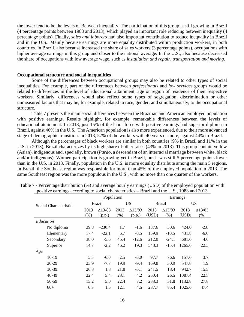
Table 7 presents the main social differences between the Brazilian and American employed population
with positive earnings. Results highlight, for example, remarkable differences between the levels of
educational attainment. In 2013, just 15% of the labor force with positive earnings had superior diploma in
Brazil, against 46% in the U.S.. The American population is also more experienced, due to their more advanced
stage of demographic transition. In 2013, 57% of the workers with 40 years or more, against 44% in Brazil.
Although the percentages of black workers are similar in both countries (9% in Brazil and 11% in the
U.S. in 2013), Brazil characterizes by its high share of other races (43% in 2013). This group contain yellow
(Asian), indigenous and, specially, brown (Pardo, a descendant of an interracial marriage between white, black
and/or indigenous). Women participation is growing yet in Brazil, but it was still 5 percentage points lower
than in the U.S. in 2013. Finally, population in the U.S. is more equality distribute among the main 5 regions.
In Brazil, the Southeast region was responsible for more than 45% of the employed population in 2013. The
same Southeast region was the more populous in the U.S., with no more than one quarter of the workers.
Table 7 - Percentage distribution (%) and average hourly earnings (USD) of the employed population with
positive earnings according to social characteristics – Brazil and the U.S., 1983 and 2013
Social Characteristic
Population Earnings
Brazil US Brazil US
2013
(%)
13/83
(p.p.)
2013
(%)
13/83
(p.p.)
2013
(USD)
13/83
(%)
2013
(USD)
13/83
(%)
Education
No diploma 29.8 -230.4 1.7 -1.6 137.6 30.6 424.0 -2.8
Elementary 17.4 -22.1 6.7 -8.5 159.9 -10.5 431.8 -6.6
Secondary 38.0 -5.6 45.4 -12.6 212.0 -24.1 681.6 4.6
Superior 14.7 -2.2 46.2 19.3 548.3 -15.4 1265.6 22.3
Age
16-19 5.3 -6.0 2.5 -3.0 97.7 76.6 157.6 3.7
20-29 23.9 -7.7 19.9 -9.4 169.8 30.9 547.8 1.9
30-39 26.8 1.8 21.8 -5.1 241.5 18.4 942.7 15.5
40-49 22.4 5.4 23.1 4.2 260.4 26.5 1087.4 22.5
50-59 15.2 5.0 22.4 7.2 283.3 51.8 1132.8 27.8
60+ 6.3 1.5 12.1 4.5 287.7 85.4 1025.6 47.4

17
Race1
White 48.6 -9.0 81.8 -9.4 289.4 -13.1 954.1 30.1
Black 8.9 2.2 11.3 1.8 171.4 25.6 716.9 30.8
Other 42.5 6.8 8.6 6.0 175.1 -5.1 984.3 36.3
Gender
Male 57.5 -11.1 53.8 -4.1 261.0 39.0 1104.0 22.3
Female 42.5 11.1 48.0 2.5 188.7 90.4 735.6 53.5
Region (Brazil/US)
North/West 6.1 3.6 21.1 2.3 198.5 12.2 968.0 26.2
Northeast 23.9 -2.3 20.9 -4.0 155.0 66.1 1028.1 39.3
Southeast 45.3 -3.4 25.0 1.7 258.5 35.0 860.0 32.1
South/Southwest 16.5 0.7 12.4 2.0 251.0 51.1 906.3 24.6
Midwest 8.2 1.4 22.4 -3.6 276.1 62.3 894.9 25.6 Source: PNAD (IBGE) and CPS (BLS).
1 Information for race in Brazil refer to 1986.
Most social groups are also submitted to higher levels of earnings inequality in Brazil. For example, in
2013, the average monthly earnings of those with superior diploma in Brazil was 3.4 times higher than that of
those with elementary diploma or less. In the U.S., it was just 2.9 times higher. The average monthly earnings
of white workers was 69% higher than that of black workers in Brazil and just 33% higher in the U.S.. The
average monthly earnings in the richest region in Brazil (Southeast) was 67% higher than in the poorest region
(Northeast), and 20% higher in the U.S. between the Northeast region, the richest, and Southeast, the poorest.
The exceptions are the earning differentials between gender and age, which are substantially higher in
the U.S.. For example, in 2013 the average monthly earnings of men was 50% higher than that of the women
in the U.S. and 38% higher in Brazil. Differences in the levels of educational attainment may help explaining
such differences, which are relatively higher for women in Brazil10. In turn, the average monthly earnings of
adults between 40 and 49 years, for example, was 6.9 higher than that of young workers between 16 and 19
years in the U.S. and just 2.7 times higher in Brazil. Differences that may be related to higher levels of intra-
generational mobility in the U.S..
Differences between the social groups followed the same dynamics witnessed for the occupational
groups: decreasing trend in Brazil and increasing trend in the U.S.. In Brazil, average earnings grew faster for
some of the most vulnerable social groups: people with elementary education or less, young between 16 and
19 and elderly with 60 years or more, black, female and those workers living in the poorest Northeast region.
In the U.S., average earnings grew faster for those with superior diploma, elderly with 60 years or more, other
races, female and those living in the richest Northeast region.
Since these social characteristics tend to be interrelated with the occupational structure, we have now
to consider the independent contribution of each factor to explain total inequality in Brazil and in the U.S..
Figure 5 presents the marginal contribution of each social characteristic, as well as that of the occupational
structure, to explain total Theil index (equation 14). The Between inequality now represents the share of the
total inequality due to the differences between the multiple combinations of groups defined by occupation,
education, age, race, gender and region. The marginal contribution of education, for example, represents the
share of the Between inequality that can be independently explained by the differences between the groups of
educational attainment, after the differences between the other groups are controlled for. The share of the
10 For example, in 2013 the percentage of employed population with positive earnings and secondary diploma or more was 16
percentage points higher for women in Brazil (62% for women and 46% for men), and just 3 percentage points higher in the U.S.
(93% for women and 90% for men).

18
between inequality that can not be independently explained by one only variable is represented by the
interaction effect.
Figure 5 - Theil T for earnings inequality within (Theil Within) and between (Theil Between) occupational
(two-digits) and social groups, employed population with positive earnings – Brazil and the U.S., 1983 to
2013 Brazil
US
Source: PNAD (IBGE) and CPS (BLS).
Results highlight, for example, that occupational structure remains as the main independent source of
Between inequality in both countries, with contribution ranging from 5 percentage points in the U.S. to 6 in
Brazil in 2013. Age and education are the second and third more relevant independent factors, contributing
jointly with more 5 percentage points in the U.S. and 7 in Brazil. Gender and regional inequality are more
relevant in Brazil, contributing jointly with 4 percentage points to total inequality (2 percentage points in the
US). Race ranked last, with 1 percentage point to explain total inequality in each country.
A remarkable difference between Brazil and the U.S. is the interaction effect, which is substantially
higher in Brazil (6 percentage points in 2013, against 1 percentage point in the U.S.). This result indicates a
higher relation between social characteristics and occupational structure in Brazil, which also play a more
important role explaining total inequality in this country. After the differences between the social and
occupational groups are controlled for, including the interaction effect, the inequality that remains within these
groups are higher in the U.S.. Phenomenon that took particular place in the 2000, when the inequality decreased
more incisively in Brazil and increased more sharply in the U.S..
Final considerations
Brazil and the U.S. are notably known by their singular levels of socioeconomic inequality. Even with
substantial improvements in the early 2000s, Brazil remains with extreme levels of inequality, significantly
higher than the U.S.. Bottom and middle groups in this country are submitted to levels of per capita income
extremely low compared to their American counterparts. A huge concentration of people in the lower bound
of the income distribution in Brazil is mainly a result of its labor market structure, which is overrepresented
by low skilled and low paid occupational groups. Top and middle income groups, such as professionals,
technical and administrative support occupations, are not representative like in the U.S..
As a result, differences between occupational groups are largely higher in Brazil, especially between
occupations in the upper and lower bounds of the occupational structure. Brazil is historically known by a
labor structure characterized by extreme levels of segmentation (Ulyssea, 2006). A small share of high skilled
workers attains better job opportunities in a more structured labor market, characterized by better access to
high technology and compliance with the labor legislation. In turn, a large majority of low skilled workers
concentrates in low paid services, farming and other routinized occupations, most of them submitted to extreme
conditions of remunerations and devoid of a series of social benefits guaranteed by the labor legislation.

19
A good news in this country is that inequality reduced substantially in the 2000s. Social benefits
explains some of this fall, but a main responsible is the labor market. Benefited by the commodity boom and
unusual economic growth in the period, labor market in Brazil produced more jobs and higher wages. Per
capita income of the poorest was benefited by important social policies implemented in the 1990s and 2000s,
such as cash transfer programs and the pension system. But labor income of the poorest also grew substantially,
pushed mainly by the appreciation of the minimum wage, which almost doubled in the period.
Labor income remains as the main source of self-reported income in households and tend to dictate the
dynamics of the total inequality. In the U.S., the share of labor income in the household is even higher and the
substantial gains of the richest workers has been the main responsible for the rise in inequality since the 1980s.
High skilled professionals and management occupations were specially benefited in this period, fact that has
been attributed to the emergence of an informational society and the lack of balance between the demand and
supply of these qualified workers.
Economic dynamics in the U.S. has shown to be highly demanding of skilled professional occupations.
In addition to management occupations, professionals were the only occupational groups who increased their
share in the American occupational structure, and some workers in these groups were especially benefited
increasing their earnings and, consequently, Between and Within inequality. In Brazil, economic growth is
still related to a decreasing participation of low bottom farming occupations and increasing participation of
middle and bottom income occupational groups, such as specialists and low services. The overall impact on
total inequality was negative, since average earnings of these latter groups are closer to the national average.
Additionally, their average earnings grew faster than the average, also contributing to reduce Within inequality.
The most vulnerable occupational groups tend to be mainly affected in periods of recession, losing
their jobs or reducing their relative wages, which contributes to increase inequality. For example, dot-com and
sub-prime crises in the 2000s affected specially the labor income of the poorest in the U.S.. In Brazil, this
group was not largely affected by international crises, since the demands for commodities continued high and
institutions, such as minimum wage, played an important role guiding the raise of the earnings in the bottom
occupational groups.
Part of the inequalities between occupational groups can be explained by the social characteristics of
their respective workers. For example, the percentage of workers with no more than secondary education is
much larger in Brazil than in the U.S., and they are mainly concentrated in the bottom occupational groups.
Inequalities between occupational and social groups, defined by education, age, race, gender and region, are
significant in both countries, and they tend also to be higher in Brazil. Nonetheless, occupational structure
remains as the main source of inequalities in both countries, even after differences between social groups are
controlled for.
Conclusions
The distribution of workers among the occupational groups has shown to be an important factor to
explain differences in the levels of inequality between Brazil and the U.S.. Earnings inequality is higher in
Brazil particularly because differences between occupational and social groups are higher in this country,
which reflect a society characterized by high levels of socioeconomic segmentation.
Moreover, changes in the occupational structure tend naturally to affect earnings distribution and,
consequently, income inequality. For example, the rise of the participation of top occupational groups tend to
increase average earnings and inequality, especially when this dynamics is not sufficiently offset by a reduction
in the earnings differentials within or between these groups. The exception would be a society where top
occupations represented the large majority of the labor structure and their average earnings were closer to the
national average. But this is still a hypothetical case, even in the U.S., where the rise of the participation of the
most representative top occupational group, professionals, has contributed substantially to increase inequality.

20
References
Acemoglu, D. & Robinson, J. A., 2012. Why nations fail: the origins of power. London: Profile.
Aoyama, Y. & Castells, M., 2002. An empirical assessment of the informational society: employment and
occupational structures of G-7 countries, 1920-2000. International Labour Review, 141(1-2), pp. 123-159.
Autor, D., Levy, F. & Murnane, R., 2003. The skill content of recent technological change: an empirical
exploration. Quarterly Journal of Economics, 118(4), pp. 1279-1333.
Banerjee, A. V. & Newman, A. F., 1993. Occupational choice and the process of development. Journal of
Political Economy, 101(2), pp. 274-298.
Blau, P. M. & Duncan, O. D., 1967. The American occupational structure. New York: John Wiley & Sons.
Bourguignon, F., Ferreira, F. H. G. & Menendez, M., 2007. Inequality of opportunity in Brazil. Review of
Income and Wealth, 53(4), pp. 585-618.
Ferreira, P. C., Pessôa, S. A. & Veloso, F. A., 2011. On the evolution of TFP in Latin America, Rio de Janeiro:
FGV, EPG: Ensaios Econômicos (Working Papers).
Furtado, C., 1986. Formação econômica do Brasil. 21 ed. São Paulo: Editora Nacional.
Galor, O., Goav, O. & Vollrath, D., 2009. Inequality in landwonership, human capital promoting institutions
and the great divergence. Review of Economic Studies, 75(4), pp. 143-179.
Hoffmann, R., 1992. Sensibilidade das medidas de desigualdade a transferências regressivas. Pesquisa e
Planejamento Econômico, 22(2), pp. 289-304.
Hoffmann, R., 1998. Distribuição de renda: medidas de desigualdade e pobreza. São Paulo: Editora da USP.
Hoffmann, R., 2006. Transferência de renda e a redução da desigualdade no Brasil em cinco regiões entre 1997
e 2004. Econômica, 8(1), pp. 55-82.
International Comparison Programa, 2011. PPPs and exchange rates, Washington: The World Bank.
Kim, C. H. & Sakamoto, A., 2008. The rise of intra-occupational wage inequality in the United States, 1983-
2002. American Sociological Review, Volume 73, pp. 129-157.
Maia, A. G., 2013. Estrutura de ocupações e distribuição de rendimentos: uma análise da experiência brasileira
nos anos 2000. Revista de Economia Contemporânea, 17(2), pp. 276-301.
Maia, A. G. & Menezes, E., 2014. Economic growth, labor and productiviy in Brazil and the United States: a
comparative analysis. Brazilian Journal of Political Economy, 2(135), pp. 212-229.
Maia, A. G. & Sakamoto, C. S., 2014. Changing family structure and impacts on income distribution: the swift
demographic transition in Brazil. Boston, Population Association of America.
Neto, L. G., 1997. Desigualdades e políticas regionais no Brasil: caminhos e descaminhos. Planejamento e
Políticas Públicas, Issue 5, pp. 42-99.
Piketty, T., 2014. Capital in the twenty-first century. Cambridge: Harvard University Press.
Pinheiro, L. et al., 2009. Retrato das desigualdades de gênero e raça. 3 ed. Brasília: IPEA.
Ribeiro, C. A. C., 2012. Quatro décadas de mobilidade social no Brasil. Revista de Ciências Sociais, 55(3),
pp. 641-679.
Rose, D. & Harrison, E. (., 2009. Social class in Europe: an introduction to the European socio-economic
classification. London: Routledge.
Saboia, J., 2010. Elasticidades dos rendimentos do trabalho em relação ao salário mínimo: a experiência de
um período recente de crescimento do salário mínimo. Economia e Sociedade, 19(2), pp. 359-380.
Ulyssea, G., 2006. Informalidade no mercado de trabalho brasileiro: uma resenha da literatura. Revista de
Economia Política, 104(4), pp. 596-618.