occurrence of bacterial regrowth and nitrification in …

OCCURRENCE OF BACTERIAL REGROWTH AND NITRIFICATION IN THE

RALEIGH DISTRIBUTION SYSTEM AND DEVELOPMENT OF AN EPANET MODEL

FOR FUTURE ASSESSMENTS

Francis A. DiGiano, Weidong Zhang, Alessandro Travaglia, Donald E. Francisco and Melissa Wood

Department of Environmental Sciences and Engineering University of North Carolina at Chapel Hill

Chapel Hill, NC 27599-7400

The research on which this publication is based was supported by funds provided by the N.C. Urban Water Consortium through the Water Resources Research Institute of The University of North Carolina.

Contents of the publication do not necessarily reflect the views and policies of the Urban Water Consortium or the Water Resources Research Institute, nor does mention of trade names or commercial products constitute their endorsement by the State of North Carolina.

WRRI Project No. 50272 April 2002

One hundred thirty copies of this report were printed at a cost of $1523.75 or $ 1 1.72 per copy.

ACKNOWLEDGMENTS

The assistance of Larry McMillan, Betty Johnson, and Carolyn Newkirk from the Raleigh Department of Public Utilities is greatly appreciated.

ABSTRACT

The main objectives of this research were to: (1) conduct an additional 12-month study (July 1999 - June 2000) of water quality in the Raleigh distribution system (previous studies covered March 1997 - May 1998 and October 1998 - August 1999) to include bacterial growth and with a focus on nitrification; (2) expand the number of sampling stations (exclusive of the finished water) &om 10 to 19 in order to include more locations with relatively high water age; ( 3 ) compare several different microbial methods for evaluation of bacterial regrowth; (4) investigate the short-term variability in bacterial counts and chloramine concentration at a selected station in the distribution system in which samples were taken every four hours on four sampling dates; (5) import the hydraulic data from the existing WATERMAX model of the Raleigh distribution system into EPANET to generate predicted tracer response curves in order to compare water age with mean constituent residence time (MCRT), a parameter developed in this research; and (6) use EPANET to compare the predicted MCRT with measured MCRT from fluoride tracer data collected throughout the distributions system by the City of Raleigh in 1998.

Ammonia concentrations leaving in the finished water exceeded 0.5 mgL on a number of sampling dates. This is a direct result of difficulties in control of the chlorine to ammonia ratio at the E. M. Johnson Water Treatment Plant (WI'P). In general, the evidence for nitrification was associated with the occurrence of very low chloramine residuals as could be expected due to the intermediate production of nitrite, which then accelerates the depletion of chloramine.

While chloramine concentrations leaving in the finished water averaged about 3.5 mg/L, eight of the 19 stations had mean values of chloramine less than 2 mg/L and several stations had residuals of less than 0.5 mg/L. Nitrification was evidenced by an increase in nitrate and a decrease in ammonia concentrations at locations within the distribution system. Low chloramine concentrations were found at locations where nitrification was not evident. Other reactions such as oxidant demand at the pipe wall and in bulk solution, autodecomposition of chloramine and catalytic reactions with iron corrosion products could be responsible.

High HPC levels, as measured by R2A agar on pour plates (R2A-PP), were generally associated with low chloramine residuals as has been observed in the previous two projects in Raleigh. However, there was large variability (several log units) in HPC at any chloramine concentration. A 0.5 log increase in HPC was noted from winter to summer months, corresponding roughly to a 15°C rise in temperature. The BDOCJ (i.e., difference between initial DOC and DOC remaining after five days) test was not precise enough to relate consumption of substrate to an increase in HPC. High HPC levels and a few occurrences of positive coliform at stations with low chloramine residuals indicate the need for better understanding of water quality in the Raleigh distribution system. The annual switch from chloramine to chlorine did not show a long-term decrease in HPC nor did it prevent nitrification in subsequent months when chloramine was again used.

The R2A-PP method gave HPC that were about one to three logs higher than either the standard plate count agar (PCA-PP) as used by Raleigh or the tlyptone glucose agar (PP-TGA) method as used by Durham. Differences between PCA-PP and TGA-PP results were not significant.

However, the R2A-PP gave counts that were less than 8% of the acridine orange direct count method. HPC enumerated using pour plate, spread plate (SP) and membrane filter (MF) techniques with R2A agar showed no significant differences.

Upon installation of a %inch bypass valve near sampling station FS6 in July 2000 to connect two pressure zones, chloramine residual increased rapidly from less than 0.2 mg/L to about 1.9 mg/L and HPC decreased by 1.4 log (23,000 to 930 CFUImL) as measured by R2A-PP method. This points to improvements that can be obtained by shortened residence times once the distribution system is better understood.

HPC (R2A-PP) and chloramine residuals at four-hour intervals for each of four sampling days showed that the distribution system is dynamic. The greatest increase in HPC was 1.2 log (1,400 to 22,000 CN/mL) and smallest was 0.4 log (1 0,000 to 23,000 CFU/mL). The greatest change in chloramine was a decrease from 1.8 to 0.52 m a . Chloramine residuals changed as a result of changes in water demand that affect residence both within the pipes and within storage tanks. However, not all of the change in HPC is easily explained by changes in chloramine concentration.

The tracer response predicted by EPANET gave an MCRT that agreed closely with the average water age that was also generated by EPANET. However, when the actual fluoride tracer response data were used to calculate the MCRT, these values were far longer than those predicted by EPANET. This discrepancy was probably the result of a distribution system model that was highly skeletonized. This prevented accurate prediction of tracer movement throughout the system, particularly in the smaller pipes that have not been included in the model. The MCRT also does not provide information about the dynamic variation in the age of water due to the residence time of storage facilities and to wide changes in pipe velocities.

The major conclusions were:

Nitrification, as indicated by a decrease in ammonia and an increase in nitrate concentrations, is a potential problem in the Raleigh distribution system.

Chloramine depletion perhaps by several different pathways led to excessive HPC at a number of the sampling stations included in this study.

Residence time is a key parameter that determines the extent to which disinfectant residual is depleted and similarly, the extent to which bacteria can regrow.

MCRT is a convenient method to quantify the results of fluoride tracer studies in distribution systems but care is needed in making comparisons with the average water age as calculated by EPANET especially for highly skeletonized network models.

TABLE OF CONTENTS

... .......................................................................................................... ACKNOWLEDGMENTS i i i

............................................................................................................................... AB S TRACT v

................................................................................................................... LIST OF FIGURES xi

LIST OF TABLES .................................................................................................................... xv

. . ......................................................................................................... LIST OF APPENDICES xvii

....................................................................................... SUMMARY AND CONCLUSIONS xix

........................................................................................................ RECOMMENDATIONS xxv

...................................................................................................................... INTRODUCTION 1

.................................................................................................. PROBLEM STATEMENT 1

................................................................................................. RESEARCH OBJECTIVES 2

........................................................................................................................ BACKGROUND 5

............................................................. NITRIFICATION IN DISTRIBUTION SYSTEMS 5

............................................................. CONTROL STRATEGIES FOR NITRIFICATION 8

CLASSIC MICROBIAL METHODS FOR ASSESSING BACTERIAL REGROWTH ....... 9

WATER DISTRIBUTION SYSTEM MODELING: WATER AGE AND WATER QUALITY ......................................................................................................................... 10

. Overview of Network Models ................................................................................... 11

Steady- vs . Dynamic Models .................................................................................... 12

................................................................................ Constituent Transport Modeling 13

Water Age Modeling ................................................................................................ 14

EPANET .................................................................................................................. 15

Calibration of Network Models ................................................................................. 16

Water Quality Predictions with Network Models ...................................................... 18

Mean Constituent Residence Time from Chemical Tracer Studies ............................ 19

............. DESCRIPTION OF RALEIGH WATER SUPPLY AND DISTRIBUTION SYSTEM 23

RAW .WATER SOURCE AND TREATMENT ................................................................ -23

STORAGE TANKS AND PUMPS IN DISTRIBUTION SYSTEM ................................... 23

EXISTING HYDRAULIC NETWORK MODEL .............................................................. 24

SAMPLING SITES ........................................................................................................... 26

ANALYTICAL METHODS ..................................................................................................... 31

SAMPLE COLLECTION .................................................................................................. 31

MICROBIAL SAMPLING ................................................................................................ 31

MICROBIAL METHODS ................................................................................................. 32

Culturable Count Methods ........................................................................................ 32

Direct Count Method ................................................................................................ 34

.................................................................................................. Total Coliform Test 35

CHEMICAL TESTING ..................................................................................................... 35

RESULT. S OF WATER QUALITY MONITORING ................................................................ 37

FINISHED WATER QUALITY ........................................................................................ 37

................................................................ ESTIMATION OF MEAN RESIDENCE TIME 39

.............................................. EVIDENCE OF NITRIFICATION FROM PRIOR STUDY 40

EVIDENCE FOR NITRIFICATION IN THIS STUDY ..................................................... 40

......................................................... Ammonia Loss; Nitrite and Nitrate Production 40

.................. Spatial and Temporal Variation in Ammonia and Nitrate Concentrations 44

................................................................................................. pH Variability in DS 49

... Spatial and Temporal Variability of Water Quality in Raleigh Distribution System 50

Improvement in Water Quality at FS6 ...................................................................... 5 8

.......................................................................................... Identification of Isolates 5 9

............................................................................ Comparison of Microbial Methods 60

... Vlll

........................ Short-term (daily) Variability in Microbial Activity and Chloramine 63

Comparisons of Important Water Quality Relationships Over Three Project Periods ...................................................................................................................... 66

RESULTS OF EPANET MODELING ...................................................................................... 69

................................ CONVERSION OF EXISTING NETWORK MODEL TO EP ANET 69

.......................................... .............................. EPANET CALIBRATION PROCEDURE ; 69

......................................................................... INPUT DATA: SYSTEM OPERATIONS 73

................................................................................. INPUT DATA: WATER DEMAND -73

............................................................................... INITIAL CALIBRATION EFFORTS -74

..................................................................................... FINAL CALIBRATION EFFORT 74

............................................................... COMPARISON OF WATER AGE AND MCRT 81

........................................................................................................................ REFERENCE S 9 1

......................................................................................... APPENDIX I . LIST OF SYMBOLS 95

APPENDIX 11 . FLUORIDE TRACER DATA AT NTNE COMMUNITY CENTER SAMPLING SITES IN 1998 TRACER STUDY ....................................................................... 99

APPENDIX I11 . COMPARISON OF FLUORIDE CONCENTRATIONS PREDICTED BY EPANET AND OBSERVED AT EACH SAMPLING STATION IN 1998 TRACER

.................................................................................................................................. STUDY 105

LIST OF FIGURES

Figure 1. Depiction of movement of water parcel for calculation of water age .............................. 14

Figure 2. Pump stations and storage tanks in Raleigh distribution system . . . . . . . . . . . . . . . . . . . . . . . . . . . . . . . . . . . . .25

Figure 3 . Locations of 20 sampling stations (inclusive of finished water) in Raleigh distribution system.. . . . . . . . . . . . . . . . . . . . . . . . . . . . . . . . . . . . . . . . . . . . . . . . . . . . . . . . . . . . . . . . . . . . . . . . . . . . . . . . . . . . . . . . . . . . . . . . . . . , . . . . . . . . . . . . . . . . . . . . . . . . . . . . . -30

Figure 4. Comparison of NH3-N concentration at all stations in DS with NH3-N concentration finished water during the project of 1996-1998 (DiGiano et al. 2000). Months with free chlorine and 12/27/1997, sampling date without finished water data, 10/27/1997 sampling date without data are excluded. . .... .. .. . .. .. ... ...... ... . . .. .. . . . . . . . . . .. ... .. .. ... . .... .... .. .. .. . . . . . . . .......... -42

Figure 5. Comparison between NO3'-N concentration at all stations in DS with NO3'-N concentration in finished water in 1996-1998 (DiGiano et al. 2000). Months with free chlorine and 12/27/1997 sampling date without finished water data are excluded. ................. 42

Figure 6. Comparison of MI3-N concentration at all stations in DS with NH3-N concentration in finished water (Data available only from Jan 2000 to June 2000). ......................................... 43

Figure 7. Comparison of NO3'- N concentration in DS at all stations with NO3'-N concentration in finished water (monthly data - July 1999 to June 2000) ...................................... ........ ....... 43

Figure 8. Spatial and temporal variability in NH3-N concentration. Stations ordered from fluoride tracer studies (Table 6); monthly data for January 2000 - June 2000 (except for free chlorination in March 2000); bar height is mean value and vertical line is one positive standard deviation. .. . . . . . . . . . . . ... .. . . .. .. . ... . . . . . .. . . .... . . ... .. . . .. .. .... . . .. . . .. . . . .. ... . . . . . . . . . . . . . . . . . . .. . . . . . . . . . .. ....... 45

Figure 9. Spatial and temporal variability in NO3'-N concentration. Stations ordered from fluoride tracer studies (Table 6); monthly data for January 2000 - June 2000 (except for free chlorination in March 2000); bar height is mean value and vertical line is one positive standard deviation. ...... ..... ..... ................................ ................ ... .. ... ......... .... . . ...... , ... . .............. 46

Figure 10. Evidence of nitrification by increase in NO3'-N concentration at two stations (CC3 and FS6) (July 1999 - June 2000) . ... .. . .. . ... . . . . . . . . . . . . . ... .. .. . . . . . . . . .. . . . . . .. . . . .. . . . . . . . . .. .. .. . . . .. . . . ... . . . . . . . . .46

Figure 11. Evidence of nitrification by increase in NO3--N and decrease in M 3 - N concentrations at low chloramine residual (July 1999 - June 2000, exclusive of March 2000 during switch to chlorine) ......... ........................... ...... ...................... ... .........,....... .................. 47

Figure 12. Evidence of both nitrification and bacterial regrowth in relationship at low chloramine residual (July 1999 - June 2000, exclusive of March 2000 during switch to chlorine) ....................... ... .... .................................................................... . ............................. 48

Figure 13. Relationship between NO3--N concentration and pH (July 1999 - June 2000, exclusive of March 2000 during switch to chlorine) .................................................. ...... ... ... 48

Figure 14. Relationship between NH3-N concentration and pH. .. . . . . . . . . . . . . . . . . . . . . . . . . . . . . . . . . . . . . . . . . . . . . . . . . . . . -49

Figure 15. Comparison of average pH measurements at each station (from July 1999 to June 2000) with UNC laboratory measurements (from February 2000 to June 2000); stations arranged in order of increasing residence time .......................................................................... 50

Figure 16. Variation in pH (fiom July 1999 to June 2000) for use of either free- or combined chlorine . . . . . . . . . . . . . . . . . . . . . . . . . . . . . . . . . . . . . . . . . . . . . . . . . . . . . . . . . . . . . . . . . . . . . . . . . . . . . . . . . . . . . . . . . . . . . . . . . . . . . . . . . . . . . . . . . . . . . . . . . . . . . . . . . . . . . .5 1

Figure 17. Spatial and temporal variability of chloramine residual in the DS (July 1999 - June 2000, exclusive of March 2000 during switch to chlorine)) . . . . . . . . . . . . . . . . . . . . . . . . . . . . . . . . . . . . . . . . . . . . . . . . . . . . . .5 1

Figure 18. Spatial and temporal variability of TOC concentration in the DS (July 1999 - June 2000) ............................ ........................................... ................. ............. . ........................ .... ........ 53

Figure 19. Spatial and temporal variability of BDOCs concentration in the DS (July 1999 - June 2000) .... ....... . ................................... ................ ... . ......... .. ........ ,. ,.. , .. ....... .. . . ..... ... . . ... ...., ... .... .. ...... 53

Figure 20. Spatial and temporal variability of HPC (R2A-PP method) in the DS (July 1999 - June 2000) .................................................................................................................................. 54

Figure 21. Comparison of HPC levels before the switch to free chlorine (February), during the switch to free chlorine (March) and after the return to chloramine (April) for 1998, 1999, and 2000 .............................................................................................. ....................................... 56

Figure 22. Relationship between log (HPC) and chloramine residual in the DS (July 1999 - June 2000, exclusive of March 2000 during switch to chlorine) ....................................................... 57

Figure 23. Relationship between log (HPC) and BDOCs in the DS (July 1999 - June 2000) ......... 57

Figure 24. Relationship between chloramine residual and BDOCs consumption in the DS (data only available for August - December 1999, February 2000 and June 2000); finished water and station FS 14 are not included. ... . . . . . . .. .... . .. . . . . .. . . . . . . . . . . . . . . . . . . . .. . . . . . . . . . . . . . .. . . . .. . . . . . . . . . . . . . . . . . . . . . . . . .. . .5 8

Figure 25. Chloramine concentration and HPC (R2A pour plate) at FS6 for twenty sample dates covering the period before and after the installation of the 2-inch bypass valve near FS6 . . .... .59

Figure 26. Comparison of PCA-PP, TGA-PP, and R2A-PP Results at FS6 (May 2000-October 2000) ............. ............ . .. ............................... ..... .... .............. . .......... .. . . .. .. .. ... .... . .. . .... . ...... . ... . ... . .. - 5 2

Figure 27. Comparison of R2A-PP, R2A-SP, and R2A-MF results at FS6 (May 2000-October 2000) ........ ... ........... ....... .......... .................... .......,...... ......... .....,., .... . . ... ....... ..... . .. ... ...... .. ... . ......... 62

Figure 28. Comparison of the AODC and R2A-PP results at FS6 (May 2000-October 2000) ........ .63

Figure 29. Box and whisker plot to compare microbial methods for samples taken at FS6 (May 2000 to October 2000). ...................... .. ..... ..... .. . .. . .... .............. . ...... . ............ ........ . .... ...... .. . . . ... . .. . .64

xii

Figure 30. Daily variability in HPC (R2A pour technique) at FS 18 on four sampling dates . . . . . . . . . . .64

Figure 3 1. Daily variability in AODC at FS 18 on four sampling dates . . . . .. .. . . . . . .. . .. ... . .... . . . . .. .. . . . . . . .. 65

Figure 32. Daily variability in chloramine concentration at FS 18 on four sampling dates . . . . . . . . . . . . . .65

Figure 33. Relationship between log (HPC) and chloramine residual in the DS for the data for all three projects (March 1997 to June 2000) (free chlorine months are not included) ................. 67

Figure 34. Regression analysis of log (WC) with chloramine residual in the DS after pooling the data from all three project periods (March 1997 to June 2000) ..... ......................... ........ ........ 67

Figure 35. Variation of HPC at three sampling stations in the DS during all three projects with exception of free chlorination months (March 1997 to June 2000) ......................................... 68

Figure 36. Pump stations and storage tanks in Raleigh distribution system ................................... 71

Figure 37. Demand patterns for wholesale users (a) Cary pump station no. 1 (b) Cary pump station no. 2 and (c) Garner, Knightdale and Wake Forest ............ . .. ............ ....... ................... 75

Figure 3 8. Comparison of EPANET predictions and field observations for Highway 54 storage tank (595 level) with assumption of WSD varying with time ................................................. 76

Figure 39. Comparison of EPANET predictions and field observations for Fairground (595 level) with assumption of WSD varying with time ................................................................. 76

Figure 40. Comparison of EPANET predictions and field observations for Bain (495 level) with assumption of WSD varying with time .................................................................................. 77

Figure 41. Comparison of EPANET predictions and field observations for Chamberlin (495 level) with assumption of WSD varying with time ................................................................. 77

Figure 42. Comparison of EPANET predictions and field observations for North Hills (495 level) with assumption of WSD varying with time ................................................................. 78

Figure 43. Comparison of EPANET predictions and field observations for New Hope (495 level) with assumption of WSD varying with time .............. . .................................................. 78

Figure 44. Comparison of EPANET predictions and field observations for Strickland (605 level) with assumption of WSD varying with time .......................................................................... 79

Figure 45. Comparison of EPANET predictions and field observations for Six Forks (605 level) with assumption of WSD varying with time .......................................................................... 79

Figure 46. Comparison of EPANET predictions and field observations for Leesville (level 65 5) with assumption of WSD varying with time .......................................................................... 80

... Xll l

Figure 47 . Comparison of EPANET predictions and field observations for Springdale (655 level) with assumption of WSD varying with time ................................................................. 80

Figure 48 . Fluoride tracer pattern at the E.M. Johnson WTP ......................................................... 82

Figure 49 . EPANET predictions of tracer response at Millbrook Station for simulations of negative step and actual stimuli at E . M . Johnson WTP ......................................................... 83

Figure 50 . EPANET predictions of tracer response at Optimist Station for simulations of ......................................................... negative step and actual stimuli at E . M . Johnson WTP 83

Figure 5 1 . EPANET predictions of tracer response at Pullen Station for simulations of negative ....................................................................... . . step and actual stimuli at E M . Johnson WTP 84

Figure 52 . Comparison of MCRT for actual- and negative-step stimulus both fiom EPANET simulations ............................................................................................................................ 85

Figure 53 .

Figure 54 .

Figure 5 5 .

Figure 56 .

Figure 57 .

Figure 58 .

Simulated water age at Southgate Station .................................................................... 85

Comparison of average water age and MCRT. both calculated from EPANET ............ 86

Predicted versus observed fluoride concentration at Walnut Station ............................ 87

Predicted versus measured fluoride concentration at Southgate Station ........................ 88

Comparison of MCRT determined from the simulations and field.measurements ........ 89

Location of sampling stations in relation to pipes included in Raleigh network mode1 . 89

xiv

LIST OF TABLES

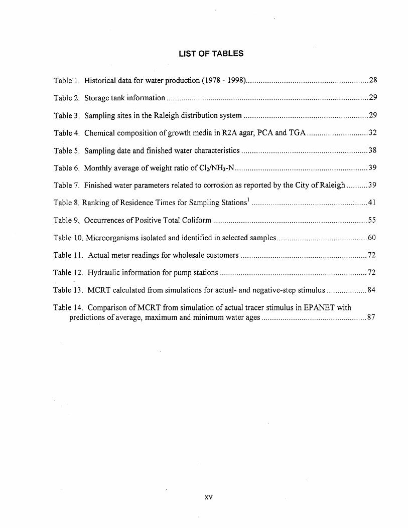
.......................................................... Table 1 . Historical data for water production (1 978 . 1998) 28

................................................................................................ Table 2 . Storage tank information 29

Table 3 . Sampling sites in the Raleigh distribution system ........................................................... 29

............................. Table 4 . Chemical composition of growth media in R2A agar, PCA and TGA 32

............................................................ Table 5 . Sampling date and finished water characteristics 38

Table 6 . Monthly average of weight ratio of C12/NH3-N ............................................................... 39

Table 7 . Finished water parameters related to corrosion as reported by the City of Raleigh .......... 39

1 Table 8 . Ranking of Residence Times for Sampling Stations ....................................................... 41

Table 9 . Occurrences of Positive Total Coliform .......................................................................... 55

Table 10 . Microorganisms isolated and identified in selected samples ........................................... 60

Table 11 . Actual meter readings for wholesale customers ............................................................ 72

Table 12 . Hydraulic information for pump stations ...................................................................... 72

Table 13 . MCRT calculated from simulations for actual- and negative-step stimulus ................... 84

Table 14 . Comparison of MCRT from simulation of actual tracer stimulus in EPANET with predictions of average. maximum and minimum water ages .................................................. 87

LIST OF . APPENDICES

APPENDIX I . LIST OF SYMBOLS ......................................................................................... 95

APPENDIX I1 . FLUORIDE TRACER DATA AT NINE COMMUNITY CENTER SAMPLING SITES IN 1998 TRACER STUDY ................................................................ 99

APPENDIX 111 . COMPARISON OF FLUORIDE CONCENTRATIONS PREDICTED BY EPANET AND OBSERVED AT EACH SAMPLING STATION IN 1998 TRACER STUDY ................................................................................................ -105

xvi i

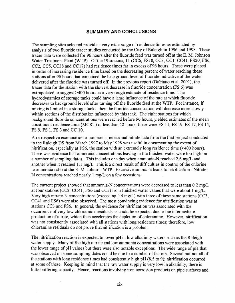
SUMMARY AND CONCLUSIONS

The sampling sites selected provide a very wide range of residence times as estimated by analysis of two fluoride tracer studies conducted by the City of Raleigh in 1996 and 1998. These tracer data were collected for 96 hours after the fluoride feed was turned off at the E. M. Johnson Water Treatment Plant (WTP). Of the 19 stations, 1 1 (CC6, FS 18, CC3, CC 1, CC4 1, FS20, FS6, CC2, CC5, CC38 and CC17) had residence times far in excess of 96 hours. These were placed in order of increasing residence time based on the decreasing percent of water reaching these stations after 96 hours that contained the background level of fluoride indicative of the water delivered after the fluoride was turned off In the previous report @iGiano et al. 2001), the tracer data for the station with the slowest decrease in fluoride concentration (FS 6) was extrapolated to suggest >400 hours as a very rough estimate of residence time. The hydrodynamics of storage tanks could have a large influence of the rate at which fluoride decreases to background levels after turning off the fluoride feed at the WTP. For instance, if mixing is limited in a storage tanks, then the fluoride concentration will decrease more slowly within sections of the distribution influenced by this tank. The eight stations for which background fluoride concentrations were reached before 96 hours, yielded estimates of the mean constituent residence time (MCRT) of less than 52 hours; these were FS 1 1, FS 19, FS 17, FS 14, FS 9, FS 1, FS 3 and CC 10.

A retrospective examination of ammonia, nitrite and nitrate data from the first project conducted in the Raleigh DS from March 1997 to May 1998 was useful in documenting the extent of nitrification, especially at FS6, the station with an extremely long residence time 0400 hours). There was evidence that ammonia concentrations leaving in the finished water were too high on a number of sampling dates. This includes one day when ammonia-N reached 2.6 mg/L and another when it reached 1.1 mg/L. This is a direct result of difiiculties in control of the chlorine to ammonia ratio at the E. M. Johnson WTP. Excessive ammonia leads to nitrification. Nitrate- N concentrations reached nearly 1 mglL on a few occasions.

The current project showed that ammonia-N concentrations were decreased to less than 0.2 mgL at four stations (CC3, CC41, FS6 and CC5) from finished water values that were about 1 mg/L. Very high nitrate-N concentrations (exceeding 0.4 mglL) with three of these same stations (CC3, CC41 and FS6) were also obserired. The most convincing evidence for nitrification was at stations CC3 and FS6. In general, the evidence for nitrification was associated with the occurrence of very low chloramine residuals as could be expected due to the intermediate production of nitrite, which then accelerates the depletion of chloramine. However, nitrification was not consistently associated with all stations with long residence times; therefore, low chloramine residuals do not prove that nitrification is a problem.

The nitrification reaction is expected to lower pH in low alkalinity waters such as the Raleigh water supply. Many of the high nitrate and low ammonia concentrations were associated with the lower range of pH values but there were also notable exceptions. The wide range of pH that was observed on some sampling dates could be due to a number of factors. Several but not all of the stations with long residence times had consistently high pH (8.5 to 9); nitrification occurred at some of these. Keeping in mind that the raw water supply is very low in alkalinity, there is little buffering capacity. Hence, reactions involving iron corrosion products on pipe surfaces and

xix

autodecomposition of chloramine could lower the pH greatly while reactions involving cement- line surfaces could increase the pH. Examining pH trends with residence time may not capture the importance of pipe materials.

Large depletions in chloramine residuals occurred in the Raleigh system. While the average chloramine concentration of finished water is 3.5 m a , eight of the 19 stations had mean values of chloramine less than 2 m a . FS18, CC3, CC14, FS6, and CC5 all had mean chloramine residuals of 1 mg/L or less. The additional nine stations added further evidence to the two earlier studies of the Raleigh distribution system. Stations with the lowest chloramine residuals were associated with long residence times. However, there were also a number of other stations having with long residence time but at which chloramine residuals were between 1 and 2 m a . There was also substantial temporal variability in chloramine residuals indicating the dynamic nature of reactions in distribution systems caused by seasonal effects, including perhaps changes in water demand that affect residence time. Low chloramine residuals in the distribution system can result from reactions that are unrelated to nitrification. Oxidant demand at the pipe wall and in bulk solution, autodecomposition of chloramine and catalytic reactions with iron corrosion products are possible explanations. The occurrence of low chloramine residuals is of concern given that the North Carolina regulations (Section .2000 - Filtration and Disinfection, .2002 Disinfection) require that the residual disinfectant shall not be less than 2.0 mg/L as combined chlorine in more than five percent of the sample each month. In this regard, sampling stations that are representative of the range of conditions in the distribution system should be selected.

In general, high HPC levels, as measured by the R2A method using pour plates, were associated with low chloramine residuals as could be expected and has been observed in the previous two projects. However, the variability in HPC at any chloramine concentration is very large (several log units). Thus, factors other than residual chloramine concentration may explain the level of microbial activity. As examples, changes in substrate level and composition as well as temperature affect the attached growth on pipes while changes in velocity affect shearing of the attached growth.

The fact that BDOC5 was lower at CCl 0, CC3, CC1, CC41, FS6, CC2, and CC5 than in the finished water was suggestive of microbial activity within the distribution system. These stations were characterized as having relatively long residence times. However, the data were not consistent in that BDOCs at two stations with long residence time (CC3 8 and CC 17) was no lower than in the finished water. As noted in the last report (DiGiano et al. 2001), the BDOCj test is not precise at concentrations of less than about 0.5 mg/L. Only a small amount of substrate is needed to produce a measurable increase in HEX. Thus, measurements of the decrease in BDOC5 that may correspond to an increase in HPC may not be within the precision of the BDOC5 test. It is also debatable as to whether a positive or negative relationship should exist between HPC and BDOC5. A low BDOC5 could very well correspond to a high HPC at a point in the distribution system with long water age, low disinfectant residual and with significant cumulative consumption of substrate. Alternatively, a low BDOCs could correspond to a low HPC if the substrate is limiting the regrowth. A more sensitive indicator of substrate utilization is needed.

Total coliforms were detected on three of the 12 monthly samplings. ' These were noted at FS6 and CC41, two stations with relatively high HPC and very low chloramine residuals. The high

HPC levels and positive coliform occurrences at stations with low chloramine residuals indicate the need for better understanding of water quality in the Raleigh distribution system. In addition, high HPC are generally known to interfere in the total coliform test. Thus, failure to obtain a positive response in the total coliform test on other sampling dates with high HPC does not exclude their presence.

A comparison of HPC levels before, during and after the annual switch from chloramine to chlorine in March showed similar result to the previous two project periods. Free chlorination produced as much as a one-log decrease in HPC levels in the bulk water, but HPC levels in April generally returned to the values observed in February. Thus, the effect on bulk levels of HPC was only temporary. The switch from chloramine to chlorine may have inactivated biofilm bacteria but this effect cannot be assessed without measurements of HPC within the biofilm. An additional rationale for the switch is to inactivate nitrifiers. However, there was ample evidence that nitrification occurred in May and June.

This study also included a direct comparison of several different microbial count methods. The R2A agar count method using pour plates (R2A-PP) gave counts that were one to three logs higher than either the standard plate count agar (PCA-PP) as used by Raleigh or the tryptone glucose agar (TGA-PP) method as used by Durham. The acridine orange direct count (AODC) may give a better indicator of the extent of all microbial processes that occur in the distribution system. This measures the total number of cells present in the system, regardless of their viability. Less than 8% of the cells measured by AODC on average were counted as viable by R2A, the most sensitive of the commonly used methods of counting.

A rough estimate was made of the effect of temperature on regrowth based on activation energy for biochemical reactions that leads to about a doubling in growth rate for a 10°C rise in temperature. When this increase in rate constant is used to calculate HPC according to first- order growth kinetics, it yields about a 1-log increase. In this study, a 0.5 log increase in HPC was noted from winter to summer months, corresponding roughly to a 15OC rise in temperature.

Installation of a 2-inch bypass valve near FS6 in July to connect two pressure zones caused chloramine residual to increase from less than 0.1 mgL to about 1.9 mglL and HPC (R2A-PP) to decrease from 23,000 to 930 CFUlmL. This action most likely reduced residence sharply and shows that a relative simple solution exists to NPC problems when the distribution system is better understood.

Eight isolates were selected to represent different morphologies from the samples of May 24, 2000. These were planted on trypticase soy agar plates and shipped with an ice pack to Analytical Services, Inc. where the MIDI fatty acid composition technique was used to identify the isolates. The results from isolate identification From samples collected at seven stations and in finished water on one sampling date were difficult to analyze because organisms could change from day to day. Very few organisms were isolated. The identification with the greatest similarity to a database provided by Analytical Services, Inc. was for Methylobacterium extorquens that was isolated from station FS 18. This station was characterized by a relatively long residence time and often had high concentrations of heterotrophic organisms. However, the source of the essential substrate (methanol) for this organism is unknown.

xxi

Comparison of microbial methods showed that bacterial numbers measured by R2A agar on PP, spread plates (SP) and membrane filters (MF) were all about the same. The City of Raleigh currently uses the PCA method. R2A might provide a better understanding of the extent of bacterial regrowth.

Measurements of the HPC by R2A-PP at four-hour intervals for each of four sampling days showed that the distribution system is dynamic. The greatest change over a four-hour period in HPC at the station selected for this study (FS18) occurred from 8 pm to 12 am on October 12 (35,000 CFU/mL to 59,000 CF'U/mL). The HPC greatest relative change was an increase from 1,400 to 22,000 CFUImL and smallest was an increase from 10,000 to 23,000 CW/mL. As expected from the HPC results, chloramine residual was variable over these sampling intervals. The greatest change in chloramine was from 1.8 to 0.52 mgL. Chloramine residuals would change as a result of changes in water demand that affect residence both within the pipes and within storage tanks.

Seasonal variations in HPC were also shown from summarizing all of the monthly data at three stations over the period of 1997 to 2000. Both the short- and long-term variations are important from a public health perspective and should be given attention in routine sampling, especially in large and complex distribution systems such as operated by the City of Raleigh.

The mean constituent residence time (MCRT), which had been proposed as a way to quantify the results of tracer studies in distribution systems @iGiano et al. 2001), was tested directly against water age as calculated by EPANET. When EPANET was used to simulate a tracer response, the resulting MCRT from that response curve was highly correlated with the average water age generated by EPANET. The MCRT method was also shown to be valid even if the assumption of negative step stimulus is replaced by the more typical, exponential decrease in tracer concentration. This is important because the fluoride feed is most often introduced before the clearwell, which serves to equalize the negative step input. This will produce an exponential decrease in concentration rather than a step decrease. One drawback to the MCRT is that dynamic variation in the age of water due to the residence time of storage facilities and to wide changes in pipe velocities are not captured.

Fluoride tracer measurements from 12 stations in the Raleigh DS were used to calculate MCRTs and compare to those predicted by EPANET. The predicted MCRTs were found to be much shorter than that calculated from the actual fluoride responses observed in the Raleigh DS. Because sampling locations were on pipes smaller than the diameters included in this highly- skeletonized EPANET model, the measured MCRT may have been longer than predicted by EPANET. In general, a skeletonized model will predict shorter water ages and thus a more rapid decrease in fluoride concentration in such tracer studies than would be actually observed. This is because fewer pipes means fewer paths for water to travel and this would lead to higher velocity and shorter water age. However, the discrepancy may also be due to limited calibration, assumptions in the modeling effort about demand allocation and daily variations, and to hold up of fluoride in the storage tanks of the network. While the existing Raleigh network model contains only 12 inch or larger pipes, water quality models should ideally contain most pipes of the DS. In fact, the assessment of water quality is of concern in small pipes that may be more distant from the water treatment plant. To include all or most of the pipes of the network

xxii

representation of a large DS is imposing both in terms of data and time required to calibrate the model. Nevertheless, it may be essential for water quality predictions.

The conclusions may be summarized as:

Nitrification is a potential problem in the Raleigh distribution system. The chlorine to ammonia ratio used for chloramination can be adjusted to limit excess ammonia; on several dates, the chlorine to ammonia ratio was between 3.5 and 3.8 and considerably lower than recommended. However, autodecomposition of chloramine may occur more rapidly at relatively low pH (< 7) and this would provide additional ammonia for nitrification even if excess ammonia leaving in the finished water were minimized. While pH values less than 7 were not found in the distribution system, the rate of autodecomposition could still be important at locations with long residence times, especially for several stations in this study where pH was often between 7.3 and 7.5.

R2A agar gave counts that were from one- to three logs higher than either the standard plate count agar or the tryptone glucose agar. Whether the nutrient poor broth used in the R2A method and different incubation conditions allows for enumeration of more of the same organisms andor for additional organisms remains unclear. Regardless of the reason, water utilities should strongly consider adoption of the R2A method to provide a more complete indicator of bacterial regrowth.

Chloramine depletion occurs by a number of pathways besides nitrification. In fact, nitrification can be a consequence of the release of ammonia when chloramine undergoes autodecomposition. The subsequent nitrification reaction will induce further depletion of chloramine through reaction with nitrite, the intermediate product in nitrification. Corrosion reactions may also cause a loss in chloramine residual. In addition, depletion is caused by bulk water reactions of chloramine with organic matter. All of these pathways would be influenced by temperature and pH as well.

Residence time is probably the key parameter that determines the extent to which disinfectant residual is depleted and similarly, the extent to which bacteria can regrow. Fluoride tracer results showed a wide range of residence times for the 19 stations included in this study. A number of stations had residence times far in excess of 96 hours.

MCRT is a convenient method to quantify the results of fluoride tracer studies in distribution systems.

EPANET was used to simulate the fluoride concentration with time at selected stations after turning off the fluoride at the treatment plant. The MCRT resulting from these model outputs agreed closely with average water age calculated by EPANET at each station. In this simulation, the fluoride could pass only through the pipes included in the network model.

The MCRT as calculated from the actual tracer data was considerably longer than the average water age calculated by EPANET; this forced the MCRT generated by EPANET to be much smaller than calculated fiom the tracer data. The most likely reason for the discrepancy is use of a highly skeletonized network model such that the sampling points for the tracer were not on pipes within the model. Other reasons include inaccurate calibration

xxiii

of the model and failure of EPANET to account for lack of mixing in storage tanks (in these simulations, storage tanks were modeled as completely mixed).

xxiv

RECOMMENDATIONS

More information is needed on the variation of residence time at any location. The factors that influence residence time are: distance fiom the WTP, water demand, storage tank operation, extent to which transmission lines are oversized, and the location of real and artificial (by closed valves) dead ends.

The variability in residence time should be examined by seasonal tracer tests and by a hydraulic model of the distribution system wherein a range of system demand conditions could be simulated. The hydraulic model may be a better tool than the tracer test because it is far less labor intensive and it permits investigation of both current and hture situations in the distribution system. Nevertheless, tracer tests are important for model calibration and for rapidly identifying areas with relatively long residence times.

Monitoring for nitrification is extremely important and requires that water utility laboratories be equipped to measure chloramine residuals, HPC bacteria, ammonia, nitrite and nitrate on a routine basis especially after identifying areas in the distribution system with long residence times. For larger water utilities with more sophisticated laboratory capabilities, ammonia- and nitrite-oxidizing bacteria may also be measured with new molecular techniques.

The R2A method should be added for monitoring the extent of bacterial regrowth even though the state regulatory agency may still only require use of the standard plate count method.

The usefblness of the MCRT, as found from tracer studies, needs to be confirmed by more comparisons with MCRT predicted from network models. In particular, tracer studies are needed in distribution systems with sampling locations on pipes with small diameters that are already included in a well-calibrated network model. Based on these first results, however, the MCRT appears to offer a simple but effective alternative to. network model estimates of water age that water utilities can calculate by conducting a tracer study without the need to develop and continuously upgrade a network model. The MCRT from a tracer study may then be used to establish a sampling network for such purposes as measurements of disinfectant residual, disinfection byproduct formation and bacterial regrowth.

Pipes having diameters of less than 12 inches need to be included in the EPANET model for the Raleigh distribution system to make it usefbl for assessing areas where water quality problems may exist. This will require more calibration effort, especially for extended periods of simulation that would cover several days of operation.

The impact of storage tank operations on water quality should be investigated by measurement of parameters such as disinfectant residual and HPC at several tank depths and at different times of day.

INTRODUCTION

PROBLEM STATEMENT

The occurrences of bacterial regrowth in the distribution system of the City of Raleigh, N.C. were documented in two previous projects (DiGiano et al. 2000 and DiGiano et al. 2001). In the first project (DiGiano et al. 2000), 15-monthly samples (March 1997 - May 1998) were collected at 10 stations and measurements were made of heterotrophic plate count (R2A agar method), total coliform bacteria, total organic carbon (TOC), assimilative organic carbon (AOC), free and combined chlorine residual, bulk water disinfectant demand, inorganic phosphorus (phosphate), inorganic nitrogen (ammonia, nitrite and nitrate), and temperature. The stations were widely scattered throughout the distribution system. Correspondingly, estimates of water age ranged from about 8 to 394 h. The second project (DiGiano et al. 2001) provided for monthly sampling at the same 10 stations for an additional 1 1 month-period (October 1998 - August 1999). The parameters included in the second project were heterotrophic plate count (R2A agar method), total coliform bacteria, TOC, biodegradable dissolved organic carbon @DOC5) (as an alternative to AOC), disinfectant concentration (free and combined chlorine), bulk water disinfectant demand, and temperature. Inorganic phosphorus (P) and nitrogen CN) were not measured in the second project primarily because A0C:N:P ratio from the field data of the first study indicated that the concentration of both nutrients was not limiting bacterial regrowth. Moreover, budget constraints and the addition of a mathematical modeling component to describe bacterial regrowth also led to elimination of the inorganic nutrient measurements.

In the first study covering March 1997 to May 1998 (DiGiano et al. 2000), a multiple, non-linear regression analysis of HPC with chloramine residual, temperature, and AOC showed that chloramine residual was the most significant independent variable. The resulting regression was: HPC (CFUImL) = 123 [Chloramine Residual ( m g / ~ ) ] ' ~ . ~ ~ ; however, the relatively low R~ value (0.35) indicated that such regression models fail to capture completely the cause and effect relationship. In the second study covering October 1998 to August 1999 (DiGiano et al. 2001), a simpler, linear relationship was tested between log HPC and chloramine concentration with the following result: log HPC (CFU/rnL) = -0.75[Chloramine Residual ( m a ) ] + 3.6; the R~ value was somewhat higher (0.47) than the previous study. It should be noted that regression analyses that include the effects of both chloramine residual and residence time on HPC were not performed because: (1) chloramine and residence time are autocorrelated and (2) residence time values were not available for each sampling staiion on each sampling date. Using the results of one tracer study to estimate residence time, a general trend of decreasing disinfectant residuals with increasing residence time was noted. However, there was considerable variation in residuals at each sampling station. For instance, the range for the mean f one standard deviation was typically more than 1 mg/L (DiGiano et al. 2001). The lowest chloramine residuals were about 0.2 mg/L at station FS6. This station is located in downtown Raleigh on the dividing line between two pressure zones. As a result, the estimated water age was the longest of all stations (394 hr). Although the study did.not include investigation of causative factors, low chloramine residual could be caused by chloramine demand exerted in water storage tanks, nitrification, autodecomposition of chloramine (Vikesland, Ozekin and Valentine 1998), and chloramine

reactions with corrosion products (Vikesland and Valentine 2000), biofilm and natural organic matter.

The first project provided evidence for the occurrence of nitrification in the distribution system. This is biochemically driven process by which two types of autotrophic bacteria are able to derive energy for growth, one by converting ammonia to nitrite and the other, by converting nitrite to nitrate. A decrease was measured in ammonia concentration and an increase in nitrite and nitrate concentrations at several stations in the Raleigh distribution system during six of the 12 monthly samplings. The consequence was also a decrease in chloramine residual and thus the potential for more bacterial regrowth. The extent of these changes was most apparent at FS6 because water reaching this station was characterized as having a very high water age.

The first project (DiGiano et al. 2000) also compared HPC by the R2A agar method (membrane filtration) to HPC by both the standard plate count agar technique (pour plates) as used by the City of Raleigh and the tryptone-glucose agar (pour plates) as used by the City of Durham. The R2A method yielded HPC that were 3 to 4 logs greater than either the TGA or PCA pour plate methods, but the ratio of the counts by R2A to either method used at these water utilities was not always the same.

Another limitation to the previous measurements of regrowth was use of methods that measured total viable counts rather than the total number of cells in the sample. These viable method techniques select for only the organisms that are acclimated to growing under the provided conditions, perhaps vastly underestimating the actual number of cells in the sample. Some organisms are likely to be dormant due to sub-optimal conditions for reproduction (Means et al. 198 1). Therefore, it would be usefbl to include a total direct count that is not dependent on such conditions.

The measurements of water quality in the Raleigh distribution system and the initiation of mathematical modeling to predict bacterial regrowth reinforced the importance of knowing the spatial and temporal variability in water age. However, the only water age data that was available fiom the City of Raleigh derived fiom interpreting data from a single fluoride tracer study conducted in October 1996. Water age can be estimated in mathematical models of distribution systems such as EPANET, a public domain software. Although the City of Raleigh does not have such model in place yet, a proprietary hydraulic network model, WATERMAX, has been used by Pitometer Associates (Cruickshank 1993) for planning purposes and maximum day analyses. Although this model does not allow calculation of water age, the information concerning pipe network characteristics (network layout, length and diameter of pipe segments, pumping stations, storage tanks, etc.) can be imported into EPANET for estimation of water age and for analysis of changes in disinfectant residuals throughout the distribution system. The critical first step, however, is calibration of the model for long term, dynamic simulations.

RESEARCH OBJECTIVES

The objectives of this research were to:

1. Conduct an. additional 1 Zmonth study of water quality in the Raleigh DS including bacterial growth with a focus on nitrification (monthly samples)

2. Expand the number of sampling stations (exclusive of the finished water) from 10 to 19 in order to include more locations with relatively high water age

3. Compare several different microbial methods for evaluation of bacterial regrowth

4. Investigate the short-term variability in bacterial counts and chloramine concentration at a selected station in the distribution system in which samples were taken every four hours on four sampling dates

5 . Import the hydraulic data from the existing WATERMAX model of the Raleigh distribution system that was calibrated in 1993 into EPANET to predict tracer curves (concentration vs. time) at various locations in response to a hypothetical tracer stimulus at the water treatment plant in order to compare water age with the mean constituent residence time (MCRT), a parameter developed in this research

6. Use the EPANET model to compare predicted MCRT and measured MCRT, the latter from fluoride tracer data that were collected at stations throughout the distribution system by the City of Raleigh in 1998 (a follow-up to the 1996 tracer study).

BACKGROUND

NITRIFICATION IN DISTRIBUTION SYSTEMS

Nitrification is a microbial process by which ammonia is converted to nitrate by autotrophic microbial bacteria:

NH: +:o, AOB >NO; + H 2 0 + 2 H '

1 NO; + - 0, NOB > No;

2

where AOB refers to ammonia oxidizing bacteria and NOB to nitrite oxidizing bacteria. Several different genera of AOB and NOB may be present although Nitrosomonas and Nitrobacter are the most often cited genera of AOB and NOB, respectively. In recent work, Regan, Hamngton and Noguera (2002) identified AOB and NOB in distribution samples through molecular biology techniques. They suggested that Nitrosomonas oligotropha and N. urea are important AOB. The NOB community comprised primarily Nitrospira although Nitrobacter was also detected. The presence of NOB suggests that both biotic and abiotic oxidation of nitrite can occur. The latter is of major concern in distribution systems because chloramine is simultaneously reduced and disinfectant residual is rapidly lost.

In wastewater treatment applications of the nitrification process, it is generally assumed that formation of nitrite is the slower of the two steps and thus, rate-limiting. If this is the case, then very little nitrite should be present because rate limiting means that once formed, it is converted to nitrate in the second step. However, studies of nitrification in distribution system have shown nitrite-N concentrations that reached 400 pg/L (Skadsen 1993; Wilczak et al. 1996; Odell et al. 1996; McGuire, Lieu and Pearthree 1999). This would suggest that the rate of nitrite formation may be faster rather than slower than the rate of nitrate formation such that nitrite accumulation is possible.

Equation 1 also shows that nitrification increases H+. The subsequent effect on pH depends on the buffer capacity of the water and other factors such as pipe materials, corrosion activity, and other biological reactions. Odell et al. (1996) suggests from surveys of water utilities that a decrease in pH may only be a good indicator of nitrification in those utilities with low buffering capacity. Such a condition would be typical, however, of many water supplies in North Carolina.

The ammonia to drive the nitrification process derives either directly or indirectly from chloramination of drinlung water. Chloramination is the intentional formation of the combined form of chlorine (chlorarnines) by addition of ammonia to free chlorine. Many water utilities have already switched from free- to combined chlorine in order to reduce formation of disinfection by-products and thus to comply with the Stage 1 DisinfectantslDisinfection By- products Rule [63 F. R. 241 (December 16, 1998)l. Combined chlorine is generally thought of

as offering a more stable form of disinfectant residual than free chlorine. However, chemical and biochemical reactions involving both the bulk water and the surface of pipes in the distribution system are of concern. These lead to release of the ammonia and subsequent nitrification.

Nitrification gives rise to several negative consequences. Foremost is the intermediate production of nitrite (NO;), an oxidant that can subsequently react with monochloramine ( W C l ) , the principal form of combined chlorine. This reduces the disinfectant residual and promotes more regrowth activity and thus higher HPC. According to the stoichiometry presented above, nitrification also leads to a decrease in alkalinity, pH and dissolved oxygen that may have negative impacts on water quality.

Of particular regulatory concern is violation of the total coliform rule. This may happen as a result of a loss disinfectant residual to which chemical reduction of chloramine with nitrite can be an important contributor. Wilczak et al. (1996) also suggested that the periodic switch to fiee chlorine to control nitrification (this is required by the State of North Carolina for one month each year) might also lead to violation of the coliform rule. The hypothesis is that coliform bacteria are released from the biofilm when free chlorine is applied. The sequence of events to produce nitrification is not clearly understood. One concept is that the chloramine concentration must first decrease due to chloramine demand reactions (both in bulk water and at the pipe wall) in order to allow nitrifying bacteria to grow. Another concept is that nitrification can occur even at relatively high chloramine concentration (1.2 to 1.5 mg/L) and subsequently, the reaction of nitrite with chloramine causes a rapid loss in residual while also liberating ammonia to produce even more nitrification. Vikesland and Valentine (2000) show that loss of monochloramine can occur due to reaction with Fe(I1) iron that may be present at the surface of cast iron pipe under conditions that favor corrosion. Vikesland, Ozekin and Valentine (1998) also suggest that autodecomposition of chloramine occurs wherein natural organic matter serves as a catalyst. In this process, ammonia can be released and thus, nitrification would be encouraged. Once the nitrification process is occurring, very high dosages of chlorine (5 - 6 m a ) are reported as necessary to inactivate these autotrophic organisms (Wilczak et al. 1996).

Details of the chemistry of chlorine reactions with ammonia can be found in many textbooks, e.g., Snoeyink and Jenkins (1980). There are many possible reactions and the chemistry of them is not completely understood. At the pH of chloramination (pH 7.5 to 8), the principle form of combined chlorine is monochloramine W C l ) and the reaction is:

NH, +HOCZ -+ NH,CZ+H,O (3)

The classic dose-demand curve for chlorine-ammonia reactions shows that combined chlorine forms and that the maximum combined chlorine residual is produced at molar ratio of [C12] to w3] of about 1 : 1 which corresponds to a weight ratio of [C12] to N3-w of 5: 1. Beyond this ratio, combined chlorine decreases as the additional free chlorine destroys the combined chlorine in what is referred to as the "breakpoint" reaction:

Free-residual chlorine begins to form at this molar ratio of [C12] to [NH3] which is 1 5 . Because the breakpoint reactions are more complex than shown above and depend on solution conditions, it is noted that the breakpoint molar ratio may vary from about 1.5: 1 to 2: 1. Water utilities usually express the molar ratio as a weight ratio. The range for the breakpoint molar ratio, therefore, translates to 7.5: 1 to 10: 1 where the chemical formula representations are as [C12] and m 3 - N l , respectively.

The weight ratio of [C12] to w 3 - N ] in chloramination determines the amount of unreacted ammonia that may enter the distribution system. This ratio is in the range of 3.5: 1 to 5: 1 (i.e., less than the breakpoint ratio). Snoeyink and Jenkins (1980) show that the ammonia concentration increases linearly from zero to its initial value as the [Clz] to m 3 ] molar ratio decreases from 1 : 1 (5: 1 weight ratio) to zero. Thus, combined chlorine is maximized at a weight ratio of 5: 1 while ammonia concentration is minimized. In practice, however, it is impossible to completely avoid free ammonia even when a 5 : 1 weight ratio is used. The unreacted ammonia will increase as the [C12] to m 3 - N ] weight ratio decreases. For example, based on the linear relationship between the weight ratio and ammonia unreacted, use of a weight ratio is 3.5 instead of 5: 1 results in about 30% of the applied ammonia remaining unreacted. The typical target concentration for NHzCl concentration to provide a disinfectant residual in the distribution system is 4 mg/L as C12. Given the 1: 1 stoichiometry for NHzCl formation (i.e., 5 : 1 weight ratio of C12 to NH3-N), 0.8 mg/L of NH3 would be needed. If the chloramination system were operated at a CIZ to NH3-N weight ratio of 3.5: 1 instead of 5: 1, 70% of the initial dosage of NH3 would form NH2CI and the remaining 30% would not react. Assuming the same target of 4 mgL N&Cl for disinfection would require an NH3 addition of (513.5) x 0.8 m a , or 1.14 mgL. Thus, 0.34 mg/L MI3-N (30% of the applied dosage) would enter the distribution system. It is also important to recognize that 1 mg/L loss of combined chlorine residual (as Clz) due to chemical reduction of m C l in the distribution system will release 0.21 mg/L of NH3-N.

The C12 to NH3-N ratio is important not only in control of free ammonia but also in establishing the microbiocidal activity of the chloramine. At 25"C, increasing the chlorine to ammonia weight ratio from 3: 1 to 4: 1 reduced the regrowth activity significantly in laboratory tests (Lieu, Wolfe and Means 1993). In addition, field measurements of nitrifier population in summer months in a covered reservoir of the Metropolitan Water District of Southern California showed a significant decrease when the C12 to Nil3-N ratio was in excess of 4: 1. However, a ratio of 5: 1 did not control nitrification in the Ann Arbor, Michigan, distribution system (Skadsen 1993). The confounding factor in this application appeared be that ammonia was added above the granular activated carbon filters and this induced nitrification prior to delivery of the water to the distribution system. Wilczak et al. (1996) also provide other evidence to suggest that maximizing the chlorine to ammonia weight ratio does not always solve the nitrification problem. One explanation for these observations is that ammonia can also be generated within the distribution system by reactions that involve the breakdown of monochloramine and release of ammonia through autodecomposition or reaction with ferrous iron will release ammonia (Vikesland, Ozekin and Valentine 1998; Vikesland and Valentine 2000).

The efficiency of nitrifier inactivation by combined chlorine formed at different chlorine to ammonia ratios and the potential regrowth of nitrifiers afier long exposure (weeks) was

investigated as a fhction of temperature (10, 15 and 25°C) in a laboratory study by Lieu, Wolfe and Means (1993). At all temperatures, the long exposure period following chloramination caused decreases in chloramine concentration that exceeded 80% with greater decrease at higher temperature. The effect of temperature on reaction rates is well known. In this case, the effect of low temperature on the presence of nitrifiers is two-fold: the growth rate of nitrifying organisms will be reduced but this is offset by a slower rate of disinfection. The net effect on presence of riitrifiers was slow regrowth at 10°C. Regrowth increased by a factor of about two at 15°C and again, chloramine decayed. At neither temperature, however, was the chlorine to ammonia ratio important in determining the extent of regrowth. While the initial inactivation of nitrifiers was more efficient at 25°C than at lower temperatures, regrowth was much greater.

Detection of the nitrification process within the distribution system is important for taking control steps. A rapid decrease in chloramine concentration is often observed due to its chemical reduction by nitrite. However, nitrification has also been observed even when the chloramine concentration was high (Odell et al. 1996). There may also be a several log increase in HPC levels as has been observed by Skadsen (1993). This increase is not necessarily due to the growth of nitrifiers because the simultaneous depletion of chloramine allows for all heterotrophic organisms to grow. Detection of an increase in HPC, however, is more likely with use of a more sensitive growth medium such as R2A agar instead of the standard plate count agar (Odell et al. 1996). A nitrogen balance is fairly straightforward by which the decrease in ammonia-N should equal the increase in the sum of nitrite-N and nitrate-N. However, Wilczak et al. (1996) report that the growth nitrifier organisms does not lead immediately to production of inorganic nitrogen forms but rather to organic nitrogen that is incorporated into cell growth. They suggest that production of inorganic nitrogen may not be detected until one week after nitrifiers have been established in the distribution system. Although traditional culture methods for nitrifiers are impractical as corrective action tools because of their long incubation periods, new molecular methods (Regan, Harrington and Noguera 2002) shorten the time to probably less than two days. Thus, water utility laboratories that are progressive and well equipped can rapidly measure AOB and NOB and thus more take corrective action. Measurement of a decrease in oxygen or pH is another possible indicator. However, the typical concentrations of ammonia (< 0.5 mg/L) and the stoichiometry of the nitrification reaction indicate that the decreases in oxygen and pH may too small to measure easily unless nitrification is severe.

Using field measurements from 10 utilities, Wilczak et al. (1996) provided an empirical that suggests that a nitrite-N of greater than 50 pgL is indicative of nitrification. Skadsen (1993) observed nitrite-N concentrations as high as 400 pg/L in the Ann Arbor, Mich., distribution system and McGuire, Lieu and Pearthree (1999) recorded a maximum of 250 pg/L in the Fort Worth, Texas, system. Skadsen also found that elevated HPC levels increased in proportion to nitrite-N concentrations and exceeded 10,000 cWmL at a nitrite-N of 400 p a . Temperatures above 15°C were most often needed to observe nitrification although some events were noted below 10°C.

CONTROL STRATEGIES FOR NITRIFICATION

Odell et al. (1996) provide a review of control strategies for nitrification. These authors included: (1) increase the chloramine dosage to inactivate nitrifiers; (2) maximize the chlorine to ammonia ratio to minimize the available ammonia; (3) apply free chlorination for one month per

year to inactivate nitrifiers in the biofilm of the distribution system; (4) reduce the water age storage tanks and in the distribution system to minimize the growth of nitrifiers and the loss of chloramine residual; (5) remove organic compounds that may form organic chloramines with far less bacterial inactivation potential than inorganic chloramines; and (6) flush the distribution system to control the biofilm activity. In addition to these control measures, a more recent study by McGuire, Lieu and Pearthree (1999) showed both in laboratory and field-testing that addition of chlorite (C1023 greatly inhibited the growth of nitrifiers. Chlorite could be either added as sodium chlorite or generated as a by-product of chlorine dioxide, a disinfectant. The dosage of chlorite needed for nitrifier inactivation could approach the current maximum contaminant level (MCL) under Stage 1 of the DisinfectionDisinfection by-products rule [63 F. R. 241 (December 16, 19981. However, the alternative of using free chlorine for one month per year could also lead to violation of MCLs for other disinfection by-products. The proper selection of control strategy will depend upon many factors that are specific to the combination of raw water supply, water treatment and distribution system.

CLASSIC MICROBIAL METHODS FOR ASSESSING BACTERIAL REGROWTH

Several researchers have studied different method and media combinations for enumerating bacteria from drinking waters. The introduction of R2A agar in 1979 served as an impetus for several comparison studies. The R.24 with its more diverse composition of ingredients, is likely to produce a greater diversity of species. In addition, its lower concentrations of protein and carbohydrates have been shown to grow higher numbers of bacteria than the higher-nutrient formulas (Reasoner and Geldreich 1985). Because organisms native to drinking water distribution systems are acclimated to an extremely nutrient-poor environment, sudden contact with high concentrations of nutrients can actually cause osmotic shock to some organisms. The R2A agar also yields a higher percentage of pigmented colonies than does other media (Reasoner et al. 1989). Some of the ingredients may foster pronounced pigment development. The other media generally produce only white or clear colonies. No medium is likely to grow all the cells present in the sample due to the specific requirements of each species.

In addition to variations in media composition, the HPC technique employed may also affect the bacterial populations detected. The pour plate method requires the temperature of the medium to be 4S°C when it is mixed with the sample. This technique may select for more heat-tolerant species because some organisms could suffer stress or death upon contact with the melted agar, since their native environment is usually less than 25°C (Means et al. 198 1). The pour plate technique may also result in oxygen deprivation, because the organisms are embedded in the medium. Conversely, being surrounded by the medium will provide plentiful nutrients. Other advantages of the pour.plate method are that sample volumes up to 2 mL can be used, and the technique is relatively quick and easy to perform.

The membrane filter method may select for larger or stronger species due to pressures encountered during filtration (Means et al. 1981). Because the cells are separated from the medium by the filter, nutrients could be limited if the medium is too dry. With enough moisture, capillary action should provide adequate movement of the nutrients through the filter and to the cells. This method is relatively simple to perform, though it requires prolonged exposure to the air, increasing the potential for contamination. The membrane filter method has the capacity to increase the sample volume greatly over that of the pour plate method, which can be

advantageous when analyzing drinking waters that may have low levels of bacteria (APHA 1998).

The spread plate method perhaps inflicts the least amount of stress on the organisms, and since they are on the surface, growth is not likely to be limited by oxygen. -Nutrients may be in shorter supply since they are obtained fiom only one surface. Spread plates are more labor intensive and require a limited sample volume of 0.5 mL or less.

The sample volume is important because a 100-mm diameter plate must contain at least 30 countable colonies for statistical purposes. A 100 mm plate with more than 300 colonies should not be counted due to difficulty is distinguishing one colony from another. These numbers are 20 and 200 for the 60 mm plates used for membrane filter techniques. Therefore, the sample should be diluted appropriately to fall between these numbers.

Means et al. (1981) compared several plating techniques and growth media for enumerating bacteria fiom distribution systems, and found that R2A gave higher counts than PCA. Fiksdal et al. (1982) compared several media for enumeration of bacteria from both chlorinated and unchlorinated water supplies, and found that R2A gave higher counts than all other media did when incubation times exceeded seven days. A comparison was made of R2A and PCA as pour plates and membrane filter plates incubated for 10 days (Reasoner and Geldreich 1985). It was found that the R2A gave higher counts with both methods and that pour plates gave higher counts than membrane filter plates with both media. The PCA also yielded fewer species of bacteria than the R2A. The study by Reasoner and Geldreich (1985) compared plating procedures and media, and again found that R2A yielded significantly higher bacterial counts than PCA for spread, pour, and membrane filter plate procedures, and that spread and filter plates gave better results than pour plates. They also determined that R2A allowed for much better pigment development than PCA when given sufficient incubation time. The best results were obtained fiom 14 days at 20°C. A study on pigmented bacteria showed that PCA was the least productive medium for both heterotroph counts and pigmented bacteria differentiation (Reasoner et al. 1989). The same study showed that the percentage of pigmented bacteria ranged fiom 2.3 to 9.9 times higher on R2A medium than on PCA. These studies contributed to the inclusion of the R2A medium in the 1 5th edition of Standard Methods (APHA 1985). None of the above studies included a comparison of R2A with TGA, although many users of TGA consider it comparable to PCA despite the difference in the formulas.

The Acridine Orange Direct Count (AODC) is a technique in which each cell is stained and then viewed through an epifluorescence microscope (Francisco et al. 1973). This provides a measure of all cells that does not depend on their viability on a specific culture medium. Since this technique does not require an incubation time, results are obtained much more rapidly (within 30 minutes of sample collection). The disadvantage is that all cells, both dead and alive, are included in the count. AODC could provide an effective way, however, to determine if more extensive monitoring is warranted by a culture method.

WATER DISTRIBUTION SYSTEM MODELING: WATER AGE AND WATER QUALITY

The loss of disinfectant residual within the distribution system by reactions in bulk water and at the pipe surface is central to better understanding of nitrification and other related problems

concerning bacterial regrowth. Within the last five years, several different computer models have become available to predict the spatial and temporal variability in disinfectant concentration. These are all built upon hydraulic principles in network flow analysis that were developed in the 1930s by Hardy Cross (Clark and Grayman 1998). In effect, constituents dissolved within the water are transported by the fluid flow. Accordingly, the time available for reactions that involve these constituents is determined by the residence time of the water, which is often referred to as water age. The purpose of this section is two-fold: (1) review important modeling concepts related to the determination of water age and (2) relate the results of tracer studies in distribution systems to water age.

Overview of Network Models

Water age is determined by the velocity of flow in each segment of the pipe network. The factors that most influence water velocity are: water demand and its temporal variability; operating rules for water storage tanks; and pipe characteristics (length, diameter, material and age). Because water demand is variable throughout the day and seasonally, water age will also be variable on both of these time scales. Water age is extremely long in pipes with very low flow, while it is short in mains supplying areas characterized by large consumption. Storage tanks can greatly increase water age. Water has the potential to reside in storage tanks for long periods of time due to low inflows/outflows and to poor mixing conditions. Studies of the effect of storage indicate that tanks can have a detrimental effect on water quality (Grayman and Clark 1993; Kennedy et al. 1993). Although the simplest and most common assumption is that storage tanks are completely mixed, this does not usually represent actual conditions. Instead, dead space exists in most storage tanks that can lead to long water residence times.

Pipe characteristics also impact velocity and thus, residence time. The friction loss, which is a determinant of velocity, increases with pipe length and with the inverse of pipe diameter. While length and diameter are usually known, the roughness of the pipe wall is not. Several coefficients are commonly used to account for friction. These include the C factor, Darcy- Weisbach, Chezy-Manning and Colebrook-White coefficients. These coefficients depend not only upon pipe material (e.g., cast iron, ductile iron or plastic) but age and condition of the pipe. The C factor is used in EPA.NET. Given that the pipe network comprises hundreds of pipe segments, it is not possible to' measure C factors for each. Instead, C factors must be assigned based on empirical knowledge of the distribution system; proper calibration of the hydraulic component of network models depends to a large extent on these C factors. In many older pipes, which are most often made of cast iron, tuberculation causes a significant decrease in pipe diameter. Thus, the actual diameter may not be known. This introduces another adjustment in the roughness factor to account for a decrease in the nominal pipe diameter. However, the nominal pipe diameter is still entered into the hydraulic model. Thus, the corresponding impact of tuberculation on velocity is not accounted for and this can have serious implications for water quality predictions.

The hydraulic model is set up by representing the network components as a collection of links connected together at their end points by nodes. Water flows along links and enters or leaves the system at nodes. Links consist of pipes, pumps and control valves. Nodes consist of pipe junctions, reservoirs and storage tanks. Junctions are nodes where links connect together and where water consumption occurs.

Storage facilities are defined in hydraulic network models as either as tanks or reservoirs. These definitions should not be construed as general to the water supply field. . A tank is a component of the model and its total head reflects demand and pressure conditions in the actual network. Tanks are characterized by their diameter, minimum and maximum operating level, and by their overflow level. When operating conditions in the system are such that water in a tank reaches either the overflow or the minimum level, the model may shut down the pipe connecting the tank to the network (in effect, this functions as an altitude valve). On the other hand, reservoirs (these are also referred to as headpoints orfixedgrade nades) are fixed total head boundaries for the network (Rossman 1994). Hence, a reservoir holds to its specified value of total head independently from the hydraulic and consumption conditions to which the system is subject. The total head (TH) of the storage tanks within a pressure zone (i.e., their water level) significantly influences the TH of the nodes within that zone. Typically, clearwells are modeled as reservoirs in network modeling.

A time pattern can be applied to the TH of a reservoir in order to model water level variations during the simulation. The time pattern is composed of a sequence of multipliers by which the average ("base" in modeling jargon) value of TH is multiplied. A different multiplier is used for each time period of the simulation so that the total head of a reservoir can vary as desired at each time step of the simulation.

A network model has two components: a network solver that performs calculations and a data set that describes the specific system (Cesario 1995). The network solver is the computer program that performs the hydraulic and water quality simulations and that calculates the important parameters such as flows, pressures and chemical concentrations. The data set is the input to the network solver and it comprises all the information required to specify the properties of each element characterizing the distribution system. There are three main classes into which an element of the network can be classified: (1) network components (pipes, storage tanks, reservoirs, pumps and valves); (2) operation data (control rules by which pumps and valves are turned on and off depending on the pressures in the system); and (3) consumption data (demand of water in the distribution system and its allocation to each point of the system).

Steadv- vs. Dvnamic Models .

The simplest distribution system models are steady state. Water age and the movement of both conservative and reactive constituents within the network are calculated for a constant set of operating and loading conditions. Rossman and Boulos (1993) summarize several mathematical algorithms used by steady-state models to describe mass conservation of the constituents at the nodes of a network. The disadvantage of steady-state models, however, is that they represent exclusively static hydraulic conditions, an unrealistic situation in typical distribution systems.

The factors affecting the dynamic conditions of the network are daily variations in demand, changes in storage tank water levels, pump and valve operations. All of these elements have a considerable effect on water age and water quality (Reddy, Ormsbee and Wood 1995). Dynamic models can perform extended-period simulations (EPS) that are able to predict the system behavior for many consecutive time periods. As originally developed, dynamic models are used to determine velocities and flow directions in all the pipes of the network by executing an EPS Wossman and Boulos 1993). The EPS is a series of consecutive steady-state hydraulic

simulations based on undivided pipe lengths and performed at fixed time steps. Flow, demand patterns and system operations remain constant during each hydraulic time step. Numerous references are available in the literature describing the set of equations and solution techniques used by network models to perform hydraulic extended period simulations (Rossman 1994; Cesario 1995). The dynamic water quality model uses the flows from the hydraulic analysis to solve a conservation of mass equation for a constituent at each link of the network.

The original dynamic hydraulic models have been extended in recent years to predict the variation of concentration of a dissolved substance in space and time throughout the network. The transport and the reaction of a constituent within water (e.g., chlorine) are using time intervals that are smaller than for hydraulic calculations. Typically, the time step for constituent calculations is 5 minutes whereas the hydraulic time step is 30 minutes. The reason for a shorter time step is to account for relatively fast chemical kinetics, pipes of different lengths in which reaction can occur, temporal variation in source water, and temporal variations in hydraulic conditions (e.g., changes in flow direction, etc.).

Constituent Transport Modeling

Rossman and Boulos (1 993) and Rossman (1 994) have described the analytical formulation of the constituent transport problem. The conservation of mass during transport along links (i.e., pipes) is described by the classical one-dimensional advection equation with reaction. Thus, in any link ij of the network:

where cij is the concentration of substance in link ij as a hnction of distance and time (i.e., cij = cij(xij,t)); xij is the distance along link ij; qij is the (constant) flow rate in link ij at time t; Aij is the cross-sectional area of link ij; and R(cij) is the reaction rate expression. The effect of longitudinal dispersion is not included because it is usually insignificant for the hydraulic conditions and source-input patterns encountered in most distribution systems. .

Equation 5 must be solved with a known initial condition at time zero. A boundary condition must also be specified. The assumption is made that the mass entering the junction nodes mixes completely and instantaneously. The resulting equation for the junction node i where xij = 0 (i.e., beginning of a link ij) is

where the subscript (ki) is a link with flow into the head node i of link ij; Lki is the length of link ki; G; is the external source concentration entering node i; and qsi is the flow rate of the external source. The solution of Equation 6 depends on the end-node concentration of all links ki that deliver flow into the head node i of link ij. Hence Equations 5 and 6 form a set of differential

equations over all links in the network. The mass balance for variable-volume storage tanks under the assumption of complete mixing, yields:

where the subscript T designates "tank." The first summation is made over all links kT with flow into the storage tanks and the second summation is made over all links Tj with flow out of the storage tank; VT is the volume of the storage tank at time t; CT is the concentration in the storage tank at time t; q k ~ is the flow into the storage tank from link kT; and q ~ j is the flow out of the storage tank into link Tj. The assumption of complete mixing conditions within the storage tank can be relaxed through use of other mixing models such as multicompartment models.

Water Age Modeling

Although Equations 5-7 pertain to chemical constituents, they can also be used to model the changes in water age over time throughout the network. The variable, cij, is interpreted as the age of water in link ij and cr is the average age of blended water in storage tanks. The age of water parcels is modeled in EPANET as if it were a particular "property" that each parcel carries along in its journey through the distribution system, similarly to what occurs with a chemical constituent present in a certain concentration within each parcel. Both water age and chemical constituents change in time: such a change is described for a chemical constituent by its decay (or growth) rate.

The reaction rate term for water age is set equal to 1 because it represents the rate at which water age would increase for a water quality time step within the model as depicted in Figure 1.

Figure 1. Depiction of movement of water parcel for calculation of water age

4 Water Age, Ci

Distance, xij

Water Parce 1 node j

This type of reaction rate expression, R(cij) is referred to as "zero-order" such that dc/dt = K where c is water age and K is the zero-order rate constant. For any new water parcel entering the network fiom reservoirs or source nodes Gi = 0 (i.e., new water enters with age of zero). With these modifications, Equation 5 is written as:

Setting dt = 1 (i.e., one time step) and K = 1 would represent the change in water age. For example, if the water quality time step is 5 minutes, a water parcel is 5 minutes older at each subsequent water quality time step of the simulation. The water parcel in Figure 1 at node j at time step t+l is the same parcel that leaves node i at time step t with velocity v = xi and water

age ci. Given that the parcel moves through the pipe segment from node i to node j in a single water quality time step, the water age at node j will be ci +l.

A time-averaging extended period simulation model has been developed (Reddy, Omsbee and Wood 1995). The model utilizes a single set of steady-state hydraulic results (i.e., a hydraulic EPS) to compute average, minimum and maximum values of water age at each junction node in the network. If water flows from node i to node j in pipe ij, then the age of the water reaching node j is the sum of the ages at node j. This is determined by the location where water enters the pipe and the travel time through the pipe; the latter is based on the flow pattern calculated by the steady-state hydraulic analysis. The age of water at each junction is represented by a weighted average (WA):

where qi is the flow for path i; Ai is the total age (sum of age at the supply node and the travel time to the specified node). The summation terms are calculated over all links that produce flow into the node. The only unknown in Equation 9 is the age at the supply node, which is zero for reservoirs and external source nodes.

The performance of the time-averaging model has been compared to the dynamic DVEM water quality model (Reddy, Omsbee and Wood 1995). While both produce similar results for the estimation of water age, the time-averaging model is computationally simpler and more efficient for water quality simulations. The assumption within the time-averaging model that storage facilities return to their original level at the end of a simulation cycle should be carefully examined. There are many practical situations when this does not occur.

EPANET

EPANET Version 2 is the only public domain network model that includes both hydraulic and water quality simulations. Other commercial software packages are available with various features that make them somewhat more user-friendly. However, the hydraulic and constituent reaction algorithms are very similar to EPANET. The water quality simulator in EPANET uses a Lagrangian, event driven algorithm. Dynamic conditions are simulated by a series of consecutive, steady-state hydraulic time steps. Water quality is computed over a shorter time step than the hydraulic time step. Each link of the network is divided into a number of evenly- spaced volume segments that are modeled as completely mixed. A flow segment moves along

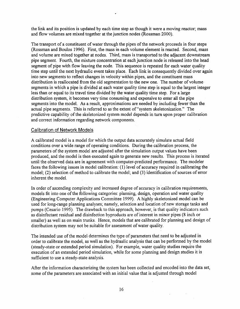
the link and its position is updated by each time step as though it were a moving reactor; mass and flow volumes are mixed together at the junction nodes (Rossman 2000).

The transport of a constituent of water through the pipes of the network proceeds in four steps (Rossman and Boulos 1996). First, the mass in each volume element is reacted. Second, mass and volume are mixed together at nodes. Third, mass is transported to the adjacent downstream pipe segment. Fourth, the mixture concentration at each junction node is released into the head segment of pipe with flow leaving the node. This sequence is repeated for each water quality time step until the next hydraulic event takes place. Each link is consequently divided over again into new segments to reflect changes in velocity within pipes, and the constituent mass distribution is reallocated from the old segmentation to the new one. The number of volume segments in which a pipe is divided at each water quality time step is equal to the largest integer less than or equal to its travel time divided by the water quality time step. For a large distribution system, it becomes very time consuming and expensive to enter all the pipe segments into the model. As a result, approximations are needed by including fewer than the actual pipe segments. This is referred to as the extent of "system skeletonization." The predictive capability of the skeletonized system model depends in turn upon proper calibration and correct information regarding network components.

Calibration of Network Models

A calibrated model is a model for which the output data accurately simulate actual field conditions over a wide range of operating conditions. During the calibration process, the parameters of the system model are adjusted after the simulation output values have been produced, and the model is then executed again to generate new results. This process is iterated until the observed data are in agreement with computer-predicted performance. The modeler faces the following issues in model calibration: (1) level of accuracy required in calibrating the model; (2) selection of method to calibrate the model; and (3) identification of sources of error inherent the model.

In order of ascending complexity and increased degree of accuracy in calibration requirements, models fit into one of the following categories: planning, design, operation and water quality (Engineering Computer Applications Committee 1999). A highly skeletonized model can be used for long-range planning analyses; namely, selection and location of new storage tanks and pumps (Cesario 1995). The drawback to this approach, however, is that quality indicators such as disinfectant residual and disinfection byproducts are of interest in minor pipes (8 inch or smaller) as well as on main trunks. Hence, models that are calibrated for planning and design of distribution system may not be suitable for assessment of water quality.

The intended use of the model determines the type of parameters that need to be adjusted in order to calibrate the model, as well as the hydraulic analysis that can be performed by the model (steady-state or extended period simulation). For example, water quality studies require the execution of an extended period simulation, while for some planning and design studies it is sufficient to use a steady-state analysis.

After the information characterizing the system has been collected and encoded into the data set, some of the parameters are associated with an initial value that is adjusted through model

calibration until the results produced by the simulation closely approximate actual field conditions. Pipe roughness coefficients - a measure of the internal roughness of pipes - and demand allocation are usually the most uncertain parameters to be adjusted during the calibration process and can be estimated by using different methods.

Extensive time-varying measurements of pressure and flow rates at selected sites in the distributions system have been used historically to calibrate the roughness coefficients in pipes. More recently, conservative constituents (tracers) such as fluoride have been employed in the calibration of water quality models. Either raising or lowering the fluoride concentration instantaneously at the water treatment plant produces a dynamic response. The parameters in the model are adjusted by matching model simulations of the tracer concentration to field- measurements through the network over time. The model is calibrated when the predicted response of fluoride at selected nodes of the network is approximately equal to the concentration- time curves fi-om the field-measurements.

Initial estimates of pipe roughness values can be obtained fi-om field experiments or from tables that provide pipe roughness as a function of material, age and diameter. The applicability of tables is limited for old pipes that are subject to tuberculation processes highly dependent on the type of water (Ormsbee and Lingireddy 1997). For this reason, it is more appropriate to obtain initial estimates of roughness coefficients through field testing in which the network is divided into areas containing pipes with the same characteristics (material and age). By conducting C- factor tests for pipes of different diameter within each zone it is possible to develop a nomograph for the entire system that shows the pipe roughness as a fbnction of pipe age for each diameter. Pipe roughness coefficients can then be assigned to all the rest of the pipes in the system by using the nomograph. Optimization methods have been developed that can be used to calibrate network models automatically by providing estimates of pipe roughness coefficients (Ormsbee and Lingireddy 1997). The most sophisticated optimization techniques make use of genetic optimization methods for the solution of complex non-linear problems.

Calibration for extended period simulations requires assignments of a temporally varying demand to each junction node. Different approaches can be used to estimate the initial spatial distribution of average demand among the network nodes. All these methods typically make use of present consumption data and service area data (Cesario 1995). Present consumption data can be determined from billing records and operations data (e.g., flow records). Service area data include the population, land use, consumption ratios and unaccounted for water. Measurements of the flow rate in trunk mains can be used to infer how water circulates in the distribution system and can be used to determine daily variations in demand.

Residential use depends primarily on the number of occupants, household income, lot size, water price, metering and climate (Buchberger and Wells 1996; Lineaweaver, Geyer and Wolff 1967). There is an intrinsic difficulty in dealing with the stochastic nature of water demand when working with the hydraulic simulation of distribution systems in which deterministic values are used to describe water consumption. New methodologies are being sought to characterize the stochastic nature of water consumption and to estimate the effects of randomness in nodal pressures (Buchberger and Wells 1996; Alegre and Coelho 1993).

The apportionment of water demand among locations within the distribution system can be very important for water quality models because spatial detail is often of interest. To obtain such data requires carefbl consideration of how water use patterns for the city under study compare to other cities for which data may be available. Moreover, the demand pattern may even vary within the city from district to district, as established in an extensive research project carried out in Lisbon, Portugal, some years ago (Alegre and Coelho 1993). In addition to water demand, leakage must be distributed both spatially and temporally. Leakage is generally allocated equally among the nodes of the network during the modeling effort and it is estimated as 10 to 15 percent of the total demand.

All possible sources of error in the input data should be identified and corrected. Any data supplied to the model could contain typographical errors (e.g., elevation equal to 750 ft instead of 570 ft) or measurement errors. Erroneous information in the data set of the system is often underestimated, thus compromising the ability of the model to predict accurately the behavior of the real system (Walski 2000). Apart from pipe roughness coefficients and system demand, other potential sources of error are: system maps, node elevations, pump curves, and incorrect valve settings or position.

While calibration is very important in the modeling effort, the state-of-the-art practice does not include a formal procedure. In the United States, standards or performance criteria that modelers should strive for have been suggested. Unlike other countries, such as the United Kingdom (Engineering Computer Applications Committee 1999), these have not been applied uniformly. The intrinsic difficulty in creating standards for calibration procedures and levels of accuracy is not surprising given the fact that the degree of accuracy needed depends on the intended use of the model. Ormsbee and Lingireddy (1997) provide a summary oY the series of steps required to calibrate a network model, while the Engineering Computer Applications Committee (1999) suggests some possible minimum criteria to calibrate hydraulic networks.

The optimization issue is one of the most debated within the modeling community. It is a useful and effective tool that can facilitate model calibration if properly used. However, it must be used in conjunction with sound engineering judgment and good data. Optimization techniques eliminate time consuming iterative manual computer runs by using an automated process but they do not require the modeler to think about the underlying reason for changing input values and for this reason, they should be used very carefully. Since optimization models are not able to distinguish between correct data and sources of error, they are likely to provide erroneous values for roughness coefficients in many situations in which the data input to the model is incorrect. The result is that a model may appear to be calibrated when, in fact, calibration was achieved by compensating errors (Walski 2000). Hence, the model may fit a particular scenario for which it has been calibrated but perform poorly when verified undersa different set of conditions.

Water Qualitv Predictions with Network Models

The only chemical constituent that has been widely modeled so far is chlorine residual. Vasconcelos et al. (1997) show that prediction of chlorine residual depends on accurate information about the hydraulics as well as the chlorine kinetics: They have reported that predicted chlorine levels were within 15 percent of the mean observed values. First-order (with

respect to chlorine concentration) kinetic constants for bulk reactions are derived fiom batch tests. Although the test is straightforward, the question remains as to whether the reaction rate is better described by including the chlorine-demanding reactants although only surrogates are available such as natural organic matter. The wall reaction is much more difficult to describe. It involves mass transfer to the surface and reaction with surface materials, e.g., with chemically reduced corrosion products. Both first-order or zero-order kinetics have been used. In either case, the rate constant is determined empirically. For example, field measurements of the decrease in chlorine concentration between two locations in the distribution system and an estimate of the bulk kinetic constant are used to fit a wall kinetic constant. Reaction at the wall can be a very important component of chlorine decay, especially for older systems that contain significant lengths of cast iron pipe. Much more fhdamental information is needed to understand the kinetics of both bulk and wall reactions of chlorine.

The results of modeling chlorine residual and other water quality parameters are often most important at locations of the distribution with very long water age. This is understandable given that long water age would correspond to long reaction time, maximum depletion in chlorine residual and thus maximum risk to consumers. However, to include locations with long water age requires a more complete detailing of pipe segments (i.e., low level of skeletonization). Not only will the model of the distribution system be more complex (more data entry), but also the calibration process must become more extensive to include the smaller diameter pipe segments for those locations with long water age.

Mean Constituent Residence Time from Chemical Tracer Studies

Chemical tracer data can be used to arrive at an estimate of the mean constituent residence time (MCRT) of water in the distribution system. It can also be used as a calibration tool within water quality models such as EPANET. The tracer must be a conservative chemical so that disappearance by reaction does not confound data interpretation. Fluoride is typically used because the feed concentration can be either increased or decreased to produce a response within the distribution system. The time required for the change in chemical concentration to be measured in a certain location of the system is related to the flow rate and to the residence time of storage tanks. A negative step input is created by suddenly interrupting the feed of fluoride into the clearwell at the WTP (DiGiano et al. 2000). The fluoride concentration at the point of injection must decrease to the background steady-state value. The feed is shut off for a period of time sufficient to measure a response at selected locations in the distribution system, where the fluoride concentration will eventually decrease reaching the background value of the water leaving the WTP.

The MCRT is estimated from the results of a tracer study using residence time distribution theory as is commonly described in reactor engineering textbooks (Weber and DiGiano 1996). At any time, t, from the moment at which the fluoride feed is interrupted at the WTP, the water at each selected location in the system is a mixture of parcels having either the original fluoride concentration prior to the negative step input, or the background fluoride concentration of the water subsequent to the negative step. Herein, "new water" stands for the water parcels containing the background concentration of fluoride entering the network after the fluoride feed is shut off, and "old water" stands for those with the original concentration of fluoride.

The mathematical expression describing the MCRT resembles a weighted average, in which the time taken by each parcel of "new water" to reach a location in the network is weighted by the corresponding fractional composition of "new water" mixing with the "old water" at the specific location. The mean travel time of water to any point in the distribution system is given by

where t, is the MCRT and t is the time elapsed from the negative step input. F(t) is the fractional composition of "new water" mixing with the water containing the original composition of fluoride (prior to the step input) at the selected location. For a negative step input F(t) is given by

[Fluoride] ,,,,, - [Fluoride], F(t) =

[Fluoride] ,,,, - [Fluoride],

where pl~oride],,~,,l is the concentration of fluoride before the fluoride feed is discontinued, [Fluoridelf is the fluoride concentration at any time t after discontinuation of the feed and pluorideIs is the background concentration of fluoride that will eventually be reached. Water is sampled at each selected station at discrete intervals of time rather than continuously. Equation 10 becomes

where i is the i-th water sample and (r) is the average fractional concentration of fluoride given by Equation 1 1 over the time interval between samples.

The MCRT method is based on the contribution of multiple water parcels to the estimation of water age; hence, it is based on a weighted average. For this reason, the MCRT reflects actual conditions in the distribution system more correctly than water age, the latter relating to a single water parcel. On the other hand, because the MCRT is the average of the age of water at each point of the network, it does not capture minimum and maximum values of water age.

While the MCRT method is appealing for its simplicity, the theoretical basis of a step change in tracer concentration at the WTP is only accurate if the fluoride addition point is after the cleanvell. However, fluoride is often added ahead of the cleanvell. In this case, the mixing conditions in the cleanvell alter the step change in fluoride concentration generated at the chemical feeder and the resulting tracer input to the distribution system is an exponential rather than step decrease in concentration. The simple equations to find t, (Equation 10-12) are restricted to analysis of step input of tracer. In more formal mathematical terms, if the clearwell behaves as a completely mixed reactor, the result of a step decrease in concentration ahead of the clearwell is an exponential decrease in concentration with time leaving the clearwell. (Weber and DiGiano 1996).

Either the simple step change or the gradual change in tracer concentration can be entered as the boundary condition in network models such as EPANET. Thus it is possible to generate within EPANET a predicted response at any node in the distribution system to either a step change or gradual change in tracer concentration. Comparison of model output to field observations of fluoride concentration at different sampling locations can then be used as a way to adjust important calibration parameters. Another interesting application that has not been explored is to compare water age predictions generated by EPANET with MCRT predictions. The latter derive from the EPANET predictions of fluoride tracer concentration with time and subsequent application of Equation 12. -

DESCRIPTION OF RALEIGH WATER SUPPLY AND DISTRIBUTION SYSTEM

RAW WATER SOURCE AND TREATMENT

Raleigh withdraws water from the Falls Lake Reservoir, which is an impoundment of the Neuse River in the watershed adjacent to Durham. This system serves over 250,000 people through a distribution system of approximately 1100 miles, about 25% of which is estimated be unlined cast iron. The E. M. Johnson WTP began addition of about 3 mgL of ozone to the raw water just before this project started in July 1999; ozone was temporarily discontinued for the month of April 2000. After ozonation, the water is treated by chemical coagulation with ferric sulfate, sedimentation, chlorination and dual-media (anthracite-sand) filtration. The water then passes through clear-well storage (detention time of about 8 hours) after which secondary addition of chlorine produces a free chlorine residual of about 2 mg/L before ammonia is added to form combined chlorine prior to entering the distribution system.

Ozonation is well known to increase the biodegradability of natural organic matter. However, the fact that chlorination is still practiced ahead of the dual media filters most likely limited biodegradation within them. The extent to which ozonation could have increased the biodegradability of substrate within the distribution system over that observed in previous studies (DiGiano et al. 2000 and DiGiano et al. 2001) is not known.

The secondary addition of chlorine to produce a free chlorine residual of about 2 mg/L prior to ammonia addition would minimize formation of organo-chloramine complexes, which are unwanted because they have no disinfection power but may be measured in the test for combined chlorine. In this report, combined chlorine refers to the formation of inorganic chloramines of which the major species is presumed to be monochloramine at the target pH of 8.2 for the finished water. The disinfectant is switched to free chlorine for the month of March. The corrosion control agent is Dabcoat 22 L which contains 23% silica and 6% PO4 (Dabco Chemical, York Pem.).

Raleigh has experienced a population increase of nearly 64,000 persons, or approximately 30 percent, since 1990. The number of water billing accounts for 1998 was approximately 90,000. In addition to the internal demand, Raleigh supplies water to Cary, Garner, Knightdale, and Wake Forest (the community of Holly Springs is a wholesale customer since 1999). These wholesale customers account for approximately one fifth of the total demand. Records produced by the Public Utilities Department show that the average day demand (i.e., the total amount of water produced in a year divided by the number of days in the year) was 42 MGD in 1998. The maximum day demand (i.e., the highest yearly daily demand) for the same year was recorded in June and reached 60 MGD. The peaking factor obtained by dividing maximum day by average day has averaged 138 percent since 1960. Table 1 shows historical data on water production for the City ofRaleigh, including average day and maximum day.

STORAGE TANKS AND PUMPS IN DISTRIBUTION SYSTEM

Figure 2 is a schematic representation of the storage tanks and pumps located in the Raleigh distribution system. These' details are presented here for later use in the EPANET model of the

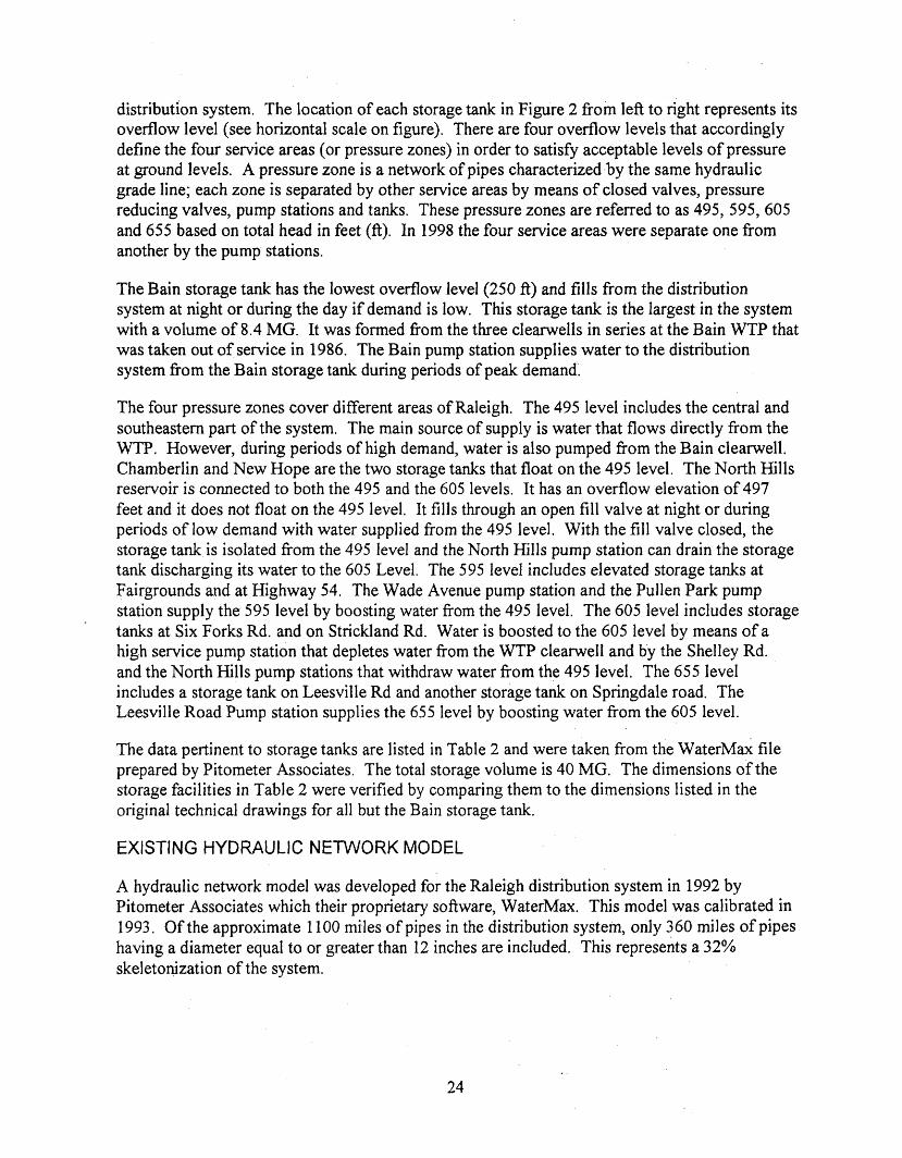
distribution system. The location of each storage tank in Figure 2 from left to right represents its overflow level (see horizontal scale on figure). There are four overflow levels that accordingly define the four service areas (or pressure zones) in order to satisfy acceptable levels of pressure at ground levels. A pressure zone is a network of pipes characterized by the same hydraulic grade line; each zone is separated by other service areas by means of closed valves, pressure reducing valves, pump stations and tanks. These pressure zones are referred to as 495, 595,605 and 655 based on total head in feet (ft). In 1998 the four service areas were separate one from another by the pump stations.

The Bain storage tank has the lowest overflow level (250 f?) and fills from the distribution system at night or during the day if demand is low. This storage tank is the largest in the system with a volume of 8.4 MG. It was formed fiom the three clearwells in series at the Bain WTP that was taken out of service in 1986. The Bain pump station supplies water to the distribution system from the Bain storage tank during periods of peak demand.

The four pressure zones cover different areas of Raleigh. The 495 level includes the central and southeastern part of the system. The main source of supply is water that flows directly from the WTP. However, during periods of high demand, water is also pumped fiom the Bain clearwell. Chamberlin and New Hope are the two storage tanks that float on the 495 level. The North Hills reservoir is connected to both the 495 and the 605 levels. It has an overflow elevation of 497 feet and it does not float on the 495 level. It fills through an open fill valve at night or during periods of low demand with water supplied from the 495 level. With the fill valve closed, the storage tank is isolated from the 495 level and the North Hills pump station can drain the storage tank discharging its water to the 605 Level. The 595 level includes elevated storage tanks at Fairgrounds and at Highway 54. The Wade Avenue pump station and the Pullen Park pump station supply the 595 level by boosting water from the 495 level. The 605 level includes storage tanks at Six Forks Rd. and on Strickland Rd. Water is boosted to the 605 level by means of a high service pump station that depletes water from the WTP clearwell and by the Shelley Rd. and the North Hills pump stations that withdraw water from the 495 level. The 655 level includes a storage tank on Leesville Rd and another storage tank on Springdale road. The Leesville Road Pump station supplies the 655 level by boosting water from the 605 level.

The data pertinent to storage tanks are listed in Table 2 and were taken from the WaterMax file prepared by Pitometer Associates. The total storage volume is 40 MG. The dimensions of the storage facilities in Table 2 were verified by comparing them to the dimensions listed in the original technical drawings for all but the Bain storage tank.

EXISTING HYDRAULIC NETWORK MODEL

A hydraulic network model was developed for the Raleigh distribution system in 1992 by Pitometer Associates which their proprietary software, WaterMax. This model was calibrated in 1993. Of the approximate 1100 miles of pipes in the distribution system, only 360 miles of pipes having a diameter equal to or greater than 12 inches are included. This represents a 32% skeletonization of the system.

Figure 2. Pump stations and storage tanks in Raleigh distribution system

I E.M. Johnson WTP Legend

Storage Tank

Pump Station

The following drawbacks to use of the existing WaterMax model for the main purposes of this research, which was to simulate a tracer study in 1998, are readily acknowledged: (1) calibration efforts have been outdated since 1993; (2) the model was calibrated only for steady-state conditions while extended-period conditions would be needed for use in water quality modeling; (3) water demand has been redistributed since 1993; and (4) the system has changed considerably owing to replacement of pumps and storage tanks. Nonetheless, the modeling exercise is still useful to illustrate the elements of calibration. In addition, this research also dealt with comparisons between water age, a parameter that is widely used, and a new parameter that we refer to as the mean constituent residence time (UCRT). Comparisons between these two parameters can be made from the output generated by a hypothetical tracer input pattern into a network model without the need for calibration.

The model was developed to provide the Public Utilities Department with a tool that would allow it to perform long range planning analyses. Its intended purpose was to assist in selecting and locating new storage tanks and pumps that would ensure acceptable levels of pressure and water supply under the most stressed conditions of demand. For this purpose, it was deemed sufficient to calibrate the model for maximum-hour conditions (i.e., the highest consumption hour during a one-hour period over the entire year). However, the applicability of the model is subsequently limited to steady-state simulations. Extension to water quality simulations would require extended period simulation under dynamic conditions.

In order to calibrate the model for maximum hour conditions, Pitometer perfiormed'extensive field measurements of pressure and flow gauging in June and September of 1992, the months of the year with highest demand. The model was then calibrated by a "trial and error" process in using WaterMax under steady-state conditions. The pipe roughness coefficients were adjusted until the predicted values of pipe velocity and the predicted hydraulic gradient at specific locations in the distribution system matched the observed field measurements. During the setting up of the model, Pitometer allocated water demand among approximately 70 percent of the nodes of the network according to the percentage of population at each node based on census tract populations from the 1990 census.

In 1997 the model was updated to include the 700 pipe segments, 12-inch and larger, that had been added between 1992 and 1997. Demand was also updated to reflect an increase in water consumption due to the new residential developments established in Raleigh between 1992 and 1997.

SAMPLING SITES

Table 3 provides a listing of the addresses for the 20 sampling sites (inclusive of the finished water) that were included. All of the 10 original sites within the distribution system (DiGiano et al. 2000; DiGiano et al. 2001) were at fire stations (FS) and the nine added sites were at community centers (CC). The location of all sites is given in Figure 3. Information to link the street address with an exact location on the skeletonized model of the distribution system as developed by Pitometer Associates was not readily available. This problem will be discussed further (see Results of EPANET Modeling). The sites were sampled monthly by city personnel from July 1999 to August 2000. Field measurements included temperature, pH, and disinfectant residual. Samples also were transported on ice to the University of North Carolina (UNC)

laboratory where they were prepared for subsequent analyses of heterotrophic plate count (HPC), chlorine (or chloramine) residual, chlorine (or chloramine) demand, total organic carbon (TOC), and biodegradable dissolved organic carbon @DOC5).

Table 1. Historical data for water production (1 978 - 1998)

Year Average Maximum Peaki.ng Factor MGD MGD w)

1978 23 32 138

1998 42 60 144 Average 138

Table 2. Storage tank information

Location Volume (MG) Overflow (ft) Minimum (ft) EMJ Plant 12 400 3 96 Clearwell Bain Clearwell North Hills Chamberlin New Hope Highway 54 Fairground Six Forks Strickl and Leesvi 11 e Springdale

Total Storage Volume

Table 3. Sampling sites in the Raleigh distribution system

Station ID' Station Address 1 EM Johnson WTP FS 11 2925 Glenridge Road, 27604 FS 19 4209 Spring Forest Road, 27609 FS 17 4601 Pleasant Valley Road, 27609 FS 14 4220 Lake Boone Trail, 27607 FS 9 4465 Six Forks Road, 27609 FS 1 220 South Dawson Street, 2760 1 FS 3 13 South East Street, 27601 FS 18 8200 Morgan's Way, 276 12 FS 20 172 1 Trailwood Drive, 27606 FS 6 2601 Fairview Road, 27608 CClO 5900 Whittier Dr. 27609 CC6 2405Wade Ave. 27607 CC 1 2615 Fitzgerald Dr. 27610 CC3 505 MLK Jr. BLvd. 27601 CC4 1 792 1 Ray Rd. 276 13 CC2 2305 Lake Wheeler Rd. 27603 CC5 1015 Halifax St. 27604 CC17 100 1 Cooper Rd. 2760 1 CC3 8 3808 ~ d i a r d s Mill Rd. 'FS indicates fire station and CC indicates community center

Figure 3. Locations of 20 sampling stations (inclusive of finished water) in Raleigh distribution system

ANALYTICAL METHODS

SAMPLE COLLECTION

Laboratory support staff of the E. M. Johnson WTP collected monthly samples fi-om the finished water (after chloramination) and from kitchen sink faucets of the fire stations and community centers (a total of 19 sites) within the distribution system. Samples were transported on ice or with ice packs both to the E. M. Johnson WTP laboratory and to the UNC laboratory where they were processed within eight hours of collection. Sampling protocol called for the sample to be taken fi-om a convenient tap after flushing at least two minutes to assure that the sample was fiom the main distribution system pipe and not the service line. This time was based on the diameter and length of the service line and the flow rate at the faucet. However, temperatures from summer month sampling in the previous two projects (DiGiano et al. 2000 and DiGiano et al. 2001) in some cases approached 29°C and this raised concerns that the flushing time was too short. Measuring temperature and chloramine concentration at various flushing times assessed the effectiveness of flushing to achieve a representative sample. Neither temperature nor chloramine concentration changed after the initial 2-minute flush for up to 20 minutes. Therefore, the amount of flushing seemed adequate to obtain a representative sample from the distribution system. A flushing time of at least five minutes was established.

MICROBIAL SAMPLING

All samples were collected in sterilized NalgeneT' 250-mL polypropylene bottles containing 1 mL 30% sodium thiosulfate. Samples for the methodology comparison experiments and short- term variability experiments (over 4-hour intervals in one day) were collected by UNC personnel and transported to the laboratory on ice.

After collecting monthly samples for about six months, sites were chosen for the microbial method comparisons and short-term variability experiments based on the monthly HPC values. For the methodology comparison experiments, a site with consistently high HPC was needed to assure that at least 30 colonies per plate could be counted with any of the enumeration methods. Site FS6 was chosen because it had an average monthly HPC of 17,000 CFU/mZ. (by the R2A pour plate method). Twenty methodology comparison experiments were conducted, spanning from May to October 2000.

Site FS 18 was selected for the short-term variability experiments because it had highly variable monthly HPC values, changing by as much as 1700 CFU/mL fiom one month to the next. Four short-term variability experiments were conducted from July to October 2000. On each date, samples were collected at 8 am, 12 pm, 4 pm, 8 pm, 12 am, 4 am, and 8 am, for a total of seven samples per experiment.

In addition to microbial analyses, temperature and chloramine was measured with a Hach DR12000 spectrophotometer.

MICROBIAL METHODS

Long-term HPC variability (month-to-month) was assessed using R2A agar on pour plates, a culturable count method which hereafter is referred to as R2A-PP. Short-term HPC variability (4-hour increments over a 24-hour period) was assessed using one culturable count method (R2A-PP) and one direct count method. The latter is referred to as the acridine orange direct count (AODC) method that measures all cells, both live and dead. In contrast, culturable count methods measure only the cells that can reproduce and make colonies under the conditions of incubation (media, temperature, oxygen, time, etc.). The methodology comparison experiments encompassed three culturable count methods [PP, spread plate (SP), and membrane filter (MF)] with three types of media (PCA, TGA, R2A), and one direct count method (AODC). The comparison of pour- and spread plate methods was of interest because both methods are used in water utility laboratories.

A single effort was made to identify some of the organisms that were cultured for HPC determinations. Eight isolates were selected to represent different morphologies fiom the samples of May 24, 2000. After isolation, these were planted on trypticase soy agar plates and shipped with an ice pack to Analytical Services, Inc. in Williston, VT. Analytical Services, Inc. using MIDI fatty acid composition technique identified the isolates.

Culturable Count Methods

Growth media for the culturable counts were prepared fiom dehydrated media (Becton Dickinson) and reagent-grade water according to section 921 5.A of Standard Methods (APHA 1998). The chemical composition of each of the three growth media is listed in Table 4.

Table 4. Chemical composition of growth media in R2A agar, PCA and TGA

R2A Agar Plate Count Agar Tryptone Glucose Agar IPCN (TGA)

15 g agar 15 g agar 15 g agar 0.5 g proteose peptone 5 g tryptone 5 g tryptone 0.5 g casamino acids

0.5 g glucose 1 g glucose 1 g dextrose 0.5 g soluble starch

0.3 g sodium pyruvate 0.5 g yeast extract 2.5 g yeast extract 3 g beef extract

0.3 g potassium phosphate 0.05 g magnesium sulfate

The glucose, dextrose, starch, and sodium pyruvate are carbohydrate sources. The yeast and beef extract are nutritional supplements, and the remaining ingredients promote pigment development in R2A (Means et al. 198 1). Differences in concentrations of these components determine which species of bacteria will be able to grow. Fifteen-rnL portions of the dissolved agar were dispensed into 30-mL glass tubes using plastic 25-mL pipettes and sterilized for 15 minutes at 121°C.

~uffered water for serial dilutions was prepared according to section 9050.C of Standard Methods (APHA-1998). The dilution water was sterilized for 15 min at 12I0C in tightly closed glass bottles. Nine-rnL portions were used for preparing dilutions for spread plates and 99 mL portions were used for preparing dilutions for pour plates. This water was also used as rinse water for the hnnel in the membrane filtration method.

Before plating, each Petri dish was labeled with the sample identifier, method, media, and sample volume. Triplicate plates of four serial dilutions were prepared for all culturable count plates. Sample was dispensed using sterile serological plastic 1-mL pipettes.

HPC were compared for the spread plate, pour plate and membrane filtration methods. Spread plates were prepared according to Section 92 15 .C of Stanhrd Methods (APHA 1998). Fifteen rnL of sterile melted medium were poured into sterile polystyrene 100 X 15 mm Petri dishes (Fisher Scientific). After the agar solidified, the plates were inverted and left to dry at room temperature until a water loss of 2-3 grams was achieved. Plates were sealed in plastic bags and stored at 4OC until time of use. A 0.1 mL sample was plated From serial dilutions so that this represented 0.1 rnL, 0.01 mL, and 0.001 mL of the original sample. After the sample was applied, a hand-spun wooden turntable was used to spin the plate while a sterile glass rod was held to spread the sample evenly across the medium surface. A control of the glass rod and method was conducted by performing the entire procedure with no sample. Another plate containing only medium was incubated to control for the plate and media.

After sterilization, tubes of media for pour plates were cooled and stored at 4°C. These were re- melted by exposure to flowing steam when needed. The melted medium was tempered to 45°C in a water bath (Model 66850, Precision Scientific) before plating. The samples were introduced from serial dilutions representing 1.0 mL, 0.1 mL, 0.01 mL, and 0.001 mL of the original sample. The procedure in section 921 5.B of StandardMethodr was used. An air quality control was performed during each pour plate session by pouring a tube of media into a plate and leaving the lid off for 15 minutes. One mL of dilution water was plated to control for the sterility of the dilution water and the pipette. Medium alone was poured into another plate to test the sterility of the media and the Petri dish. The outer surface of each tube was dried afier removing it from the water bath to prevent drips From contaminating the sample.

Membrane filter plates were prepared by pouring 5 mL of the sterile medium into 60 X 15-mm sterile polystyrene Petri dishes (Becton Dickinson). After the agar solidified, the plates were inverted, sealed in plastic bags, and stored at 4OC until used. The membrane filter method was performed according to Standard Methods section 92 15 .D. The filtration apparatus, including an Erlenmeyer flask with a vacuum arm and a Gelman filter stand and funnel, was wrapped in foil and sterilized before use. Sample volumes of 0.1 mL or 1.0 mL were filtered using serial dilutions representing 0.00 1 mL, 0.01 mL, 0.1 mL, and 1.0 mL of the original sample onto sterile 47-mm, 0.45-micron gridded membrane filters (MSI) with gentle vacuum. Sample volumes were filtered in order of smallest to largest, and the fimnel was rinsed with 20 to 30 mL of sterile dilution water between each filter. Filters were transferred using forceps sterilized in alcohol. One plate of medium with no filter was incubated to check the sterility of the medium and the plate. One dry filter was placed on the medium to control for filter sterility. One hundred mL of

the buffered rinse water was filtered and incubated to control for the sterility of the dilution water.

All plates were inverted and wrapped in plastic bags during incubation. The PCA and TGA plates were incubated in a Fisher lsotempTM incubator at 35OC for 48 hours. These conditions were selected to duplicate those used in the Durham and Raleigh utility laboratories. The R2A plates were incubated in a Precision Scientific incubator at 28°C for 7 days, according to the recommendations in Section 92 15A. 7 of Standard Methob (APHA 1998).

Colonies on spread plates and pour plates were counted manually using a Darkfield Quebec Colony Counter (American Optical Company). The dilution containing 30-300 colonies was selected for counting. The membrane filter colonies were counted using a Bausch and Lomb dissecting microscope and the dilution was selected to produce a colony density of 20-200 per filter. The average number of colonies formed for three replicate plates and the selected dilution was divided by the volume of sample in the dish and reported as colony-forming units per milliliter (CFU/mL) with two significant figures according to Section 921 5A. 8 of Standard Methoak (APHA 1998).

Direct Count Method

For the Acridine Orange Direct Count (AODC) method, glass bottles were acid-washed, rinsed with laboratory grade water, and then sterilized at 121°C for 15 minutes. A sterile 25-mL pipette was used to dispense the desired amount of sample (25-100 mL) fiom the original sample bottle to the sterile glass bottle. Particle-free 37% formalin was added to yield a final concentration of 5% formalin in the sample. Fixation allowed the samples to be stored at 4°C for one week before being filtered (APHA, 1998).

The AODC method was performed according to section 92 16.B of Standard Methods (APHA 1998). To ensure all reagents were sterile and free of particles, the formalin, rinse water and Acridine orange stain were filtered with a 0.45-p, 47-mm filter, autoclaved, and refiltered. One mL of the particle-free Acridine orange (0.1%) (Difco, Detroit, MI) was added to the sample. After staining for two minutes, it was filtered onto a black polycarbonate 0.2294 25-mm filter (OsmonicsTM) with vacuum. Ten mL of particle-free water followed to rinse the filter funnel and promote even cell distribution. The filter was allowed to dry and was placed on a drop of Cargille Type A immersion oil (Cargille Laboratories, Inc., Cedar Grove, N.J.) on a clean glass slide. Another drop of immersion oil was placed on top of the filter, followed by a 20-mm square clean glass cover slip. Immersion oil was also added to the surface of the cover slip and the filters were viewed with a Leitz Ortholux II microscope at 1250-x magnification with an epifluorescence mode barrier filter. An ocular was fitted with a grid with a measured area. A minimum of five random fields within the grid was counted to obtain a total of at least 200 cells, and then the average number of cells per grid was determined. This number was multiplied by the area of the filter (201 .O6 mm2) and divided by the area of the grid (0.00308 mm2) times the dilution factor of the fixative:

Cells / mL = (dilution. factor) x (0.003 8mm ' / grid)

The final AODC value was reported in cells/mL with two significant figures.

The sterility of the stain, water, and filtration apparatus was checked by filtering a blank of stained particle-free water. The number of cells in the blank field was subtracted from the average number of cells per field before calculating the above equation.

Total Coliform Test

The laboratory staff at E. M. Johnson WTP performed total coliform testing at the sampling sites. The colilertTM technique is used routinely.

CHEMICAL TESTING

Chlorine and combined chlorine residual were measured using a HachTM DR 2000 with the HachTM DPD colorimetric method. Throughout this report, the terminology for combined chlorine will be chloramine. At the pH of these samples (most in the range of 7.5 to 8 .9 , it is assumed from general textbook discussion such as found in Snoeyink and Jenkins (1980) that monochloramine is the principle form of combined chlorine that was present. However, measurements of individual chloramines were not made.

Two technicians fiom the E. M. Johnson WTP made field measurements of disinfectant residual, each assigned to collecting and analyzing samples from one-half of the distribution system stations. Laboratory measurements were also made of these samples at the University of North Carolina (UNC) by the same graduate research assistant. The samples were transported to UNC on ice; the maximum holding time between sampling and analysis was about six hours. Comparison of field and laboratory measurements revealed inconsistencies: samples analyzed by one field technician gave good agreement (within i 0.2 mgL) but those by the other field technician did not. Ideally, field measurements would be preferred over laboratory measurements to eliminate the time delay in which demand could be exerted. Chloramine demand measurements (48 hours at room temperature) were made upon receipt of samples in the laboratory. The mean and standard deviation of over 230 measurements for the 12 monthly samplings in this project were 0.34 and 0.29 mg/L, respectively. Thus, a small fraction of this demand would be exerted in 6 hours at a temperature far lower than room temperature. For these reasons, the laboratory measurements of chlorine and combined chlorine residual were considered a reliable substitute for field measurements.

Temperature and pH were measured using an Accumet AP6 1 portable pH meter.

Total organic carbon (TOC) analysis was performed with a Shimadzu TOC-5000 Analyzer. Samples were held at 4OC until analysis. TOC is reported because the samples were not filtered. This was justified on the basis of analysis of 10 samples fiom the Raleigh distribution system for which TOC and dissolved organic carbon (DOC) were equivalent as judged by the precision of the TOC analyzer (M.2 m a ) .

The substrate available for bacterial regrowth was measured by BDOCs test as provided by Allgeier et al. (1996). The procedure depends upon colonization of bacteria on a support medium after which water samples are placed in contact with the medium for five days. In this

research, the support medium was an open-pore sintered borosilicate (Siran) glass bead (Schott Company) having a diameter of 1-2 mm and a pore diameter of 60-300 um. The surface area (including internal area) to volume ratio of the bead is 90,000: 1. In between arrival of monthly samples, the glass beads were kept submerged in water taken from the Raleigh distribution system. Prior to analysis by the TOC analyzer, the samples were filtered through 13 mm- diameter, 0.45 pm Magna nylon filters (available through Fisher Scientific Company) that were placed into a, 5-rnL syringe filter holder made of stainless steel (also available through Fisher Scientific Company); the resulting measurements were reported as DOC. The filters were soaked overnight prior to their use in organic-free water; the filters were handled only with tweezers. When filtering a sample, one or two syringe volumes were wasted before collecting the aliquot in a clean vial. A 100-mL aliquot of each sample was dechlorinated with sodium thiosulfate and placed into a flask containing 50 mL of the sand. The flasks were shaken for 5 days, after which DOC was again measured. The BDOCs is the difference between the initial DOC and the DOC after five days. The progression of depletion of DOC over time was not measured and thus, it cannot be stated with certainty that five days was sufficient to reach a minimum DOC indicative of complete biodegradation of all substrate. The work of Allgeier et al. (1996) indicates that five days is a reasonable time period in which to achieve complete biodegradation.

The laboratory staff at the E. M. Johnson WTP performed ammonia, nitrite and nitrate analyses. EPA Method 350.1 (Determination of Ammonia Nitrogen by Semi-automated Colorimetry) was used for ammonia (U.S. EPA 1993). Alkaline phenol and hypochlorite react with ammonia to form indophenol blue that is proportional to the ammonia concentration; the applicable range is 0.0 1-2.0 mg/L NH as N. EPA Method 300.1 (ion chromatagraphy) was used for nitrite and nitrate (US. EPA 1993).

RESULTS OF WATER QUALITY MONITORING

FINISHED WATER QUALITY

The finished water quality parameters on monthly sampling dates are listed in Table 5. The variation in temperature (8 to 28OC) throughout the year is typical of previous studies (DiGiano et al. 2000; DiGiano et al. 2001). This table includes both field and laboratory measurements of chlorine residual although the latter will be used throughout the remainder of this report. The wide variation in pH (7.1 to 8.9) is not entirely explainable. The only date on which ammonia was not added is 3/28/00. Free chlorine replaces chloramination for the entire month of March as required by the State of North Carolina and consistent with this switch, the pH was fairly low (pH = 7.4) due to addition of this acid to a poorly buffered water (alkalinity<20 mgL as CaC03). If the results for 8/25/99 are disregarded for the moment, the pH for the remainder of the sampling dates varied from 7.9 to 8.9. Chloramination was being practiced on these dates and thus an increase in pH would be expected (see Equation 3). However, a variation in pH of 1 means a ten-fold variation in hydrogen ion concentration. This is not easily explainable unless difficulties were being encountered in pacing the ammonia feed to the chlorine concentration. The low pH (7.1) on 8/25/99 was most likely the result of the sample being mistakenly taken before the addition of ammonia and the final chlorination step. The evidence to support this conclusion was the much higher pH values measured at sampling stations in the distribution system near the WTP for the same day. Moreover, the total chorine concentration at these stations was much higher than 2.6 mglL as measured at the WTP.

The total chlorine concentration on sampling dates corresponding to chloramination conditions varied from 2.6 to 4.2 mg/L as measured on site. TOC varied from 2.1 to 3.2 mg/L over all sampling dates. For comparison, the mean was 2.4 mgL over the period of 3/l997 to 5/1998 (DiGiano et al. 2000) and 2.1 mglL over the period of 10/98 to 8/99 (DiGiano et al. 2001). The variation in BDOCs from 0.3 to 1.1 m a was very similar to the variations shown over a previous 1 1-month period (DiGiano et al. 200 1).

The chlorine-to-ammonia weight ratio also varied substantially (3.8 to 5.3). As noted in the Background section, this ratio will also impact the ammonia entering the distribution system: more ammonia will enter at lower ratios. The impact of chloramination on ammonia concentrations entering the distribution system is striking. For the data of record (6 monthly samples), the NH3-N concentration was about 1 mg/L during chloramination and 0.01 mg/L during free chlorination (March 28, 2000). Such high concentrations of ammonia would suggest a very large potential for nitrification and in turn, for chemical reduction in chloramine by the intermediate formation of nitrite. The variability in chlorine-to-ammonia weight ratio is also seen from the monthly average data over the study period that is given in Table 6.

Routine measurements of alkalinity and corrosivity were not included in this study. However, the E. M. Johnson WTP records provided information to show that the finished water has low alkalinity, low hardness and high corrosivity. Two results are given in Table 7.

Table 6. Monthly average of weight ratio of C12/NH3-N

Chlorine After Ammonia Weight Ratio Filtration C12/NH3-N

( W ( W Jul-99 1777 504 3.5 Aug-99 2299 503 4.6 Sep-99 2144 445 4.8 Oct-99 2070 440 4.7 NOV-99 1757 40 1 4.4 Dec-99 1465 361 4.1 Jan-00 1308 368 3.5 Feb-00 1326 348 3.8 Mar-00 863 0 0.0 Apr-00 1415 390 3.6 May-00 2085 497 4.2 June-00 2901 795 3.6

Table 7. Finished water parameters related to corrosion as reported by the City of Raleigh

Parameter Sam~le Date Value Corrosivity Ganglier Index) Alkalinity ( m a as CaC03) Total Hardness (mgL as CaC03) pH Corrosivity Canglier Index) Alkalinity (mg/L as CaC03) Total Hardness (mg/L as CaC03) DH

Norton and LeChevallier (1997) suggested the Larson Index (LI) as a usefkl way to quantify iron corrosion:

Both chloride and sulfate ions can cause pitting of metallic pipe. Based on C1' and SOm4 concentrations of 24 and 38 mg/L that were reported by the E. M. Johnson WTP (see http://raleigh-nc.org/putilities/2000wqrepo.htm), the LI is about 10. Norton and LeChevallier (1 997) suggest that LI > 1.0 would interfere with biofilm inactivation, presumably because the corrosion activity would consume disinfectant rapidly.

ESTIMATION OF MEAN RESIDENCE TIME

Prior to this study, two fluoride tracer studies were conducted in the Raleigh DS by turning off the fluoride feed at the E. M. Johnson WTP and measuring the response in the DS. These data were not adequate to calculate the MCRT by Equation 12 for all stations because the sampling

period was not sufficiently long at some station for fluoride to decrease to the background concentration. The tracer data from October 1996 were used to estimate the MCRTs of the original 10 stations and were reported earlier (DiGiano et al. 2000). Tracer data for the nine added stations were obtained in another study conducted in September 1998 and these are provided in Appendix 11. As can be seen from these plots, the fluoride concentration did not decrease to background level at some stations. This was also true for some of the original stations. For these stations, the MCRT cannot be determined accurately because the fluoride concentration-time plot would need to be extrapolated to a time when the fluoride reached the background level. To avoid extrapolation, an alternative technique was sought that would provide a relative ranlung of residence times.

Equation 11 was used to calculate the cumulative fraction of water introduced after the fluoride feed was turned off at the WRP ("new" water) that had arrived at each station after 96 hours from its introduction. Each fractional value was then converted to a percent value for ranlung of the residence time. The resulting percentage of "new" water value is listed in Table 8 for each station. The higher the percentage of this "new" water up to 96 hours, the shorter is the residence time. For those stations with 100% "new" water after 96 hours, the MCRT was calculated using Equation 12 and these values appear in the last column. Stations for which MCRT could not be calculated without extrapolation beyond 96 hours were: FS 18, FS20, FS6, CC6, CC3, CC1, CC41, CC2, CC5, CC38 and CC17.

EVIDENCE OF NITRIFICATION FROM PRIOR STUDY

Our first project in 1997-1998 included measurements of ammonia, nitrite and nitrate at ten stations in the Raleigh DS (DiGiano et al. 2000). These data were re-analyzed using the method given by Wilczak et al. (1996) to. provide additional interpretation of the evidence for nitrification. Figure 4 shows the relationship between ammonia entering the DS and ammonia within the distribution system. It should be noted that ammonia measurements were typically performed by a specific ion electrode method and therefore would not include the ammonia present in chloramine. Figure 5 is the same type of plot for nitrate. A line of 1: 1 slope is also provided in each figure. Data on this line would indicate no change within the DS whereas data points above the line would indicate production and those below the line would indicate consumption. The vertically stacked data points are for different stations in the DS on the same sampling date. Consumption of ammonia is evident from Figure 4 and similarly, production of nitrate is evident from Figure 5 on several sampling dates. These figures include one sampling date when the set point for pacing of ammonia to chlorine was incorrect, resulting in an overdose of ammonia, producing an ammonia concentration of about 2.6 mglL in the finished water.

EVIDENCE FOR NITRIFICATION IN THIS STUDY

Ammonia Loss; Nitrite and Nitrate Production

The ammonia and nitrate concentrations at each station are compared to those entering the DS in the finished water in Figures 6 and 7, respectively. According to the measurements of the laboratory staff at the E. M. Johnson WTP, nitrite was not detected in any samples over this 12- month study. Consequently, only ammonia loss and nitrate production can be assessed. Ammonia data were only available for the period of January 2000 to June 2000 whereas the

nitrate data were available from July 1999 to June 2000. As was noted in Figures 4 and 5, these data once again show the same evidence of nitrification (lower ammonia and higher nitrate concentrations in the DS than in the finished water).

Table 8. Ranking of Residence Times for Sampling stations1

Station Cumulative Percentage of MCRT ( hr) -' "New" Water up to 96 h2

FSl l 100 8 FS19 100 9 FS17 100 11 FS14 100 20 FS9 100 28 FS 1 100 30 FS3 100 52

CClO 100 52 CC6 80 - FS18 71 - CC3 58 - CC 1 5 1 - CC4 1 47 - FS20 41 - FS6 16 - CC2 12 - CC5 11 - CC3 8 5 - CC17 5 -

1 Tracer data for all FS stations was determined from fluoride tracer study of October 1996 and those for all CC stations from fluoride tracer study of September 1998 2 Calculated from Equation 1 1 3 Calculated from Equation 12 only for those stations where new water had reached 100%

Figure 4. Comparison of NH3-N concentration at all stations in DS with NH3-N concentration finished water during the project of 1996-1998 (DiGiano et al. 2000). Months with free chlorine and 12/27/1997, sampling date without finished water data, 10/27/1 997 sampling date without NH3 data are excluded.

NH3-N in Raleigh finished water (mg/L)

Figure 5. Comparison between NO3--N concentration at all stations in DS with NO3--N concentration in finished water in 1996-1998 (DiGiano et al. 2000). Months with free chlorine and 12/27/1997 sampling date without finished water data are excluded.

0.0 0.2 0.4 0.6 0.8 1.0 1.2

N03-N in Raleigh finished water (mg/L)

Figure 6. Comparison of NH3-N concentration at all stations in DS with NH3-N concentration in finished water (Data available only from Jan 2000 to June 2000).

0.0 0.3 0.6 0.9 1.2 . 1.3

Ammonia in finished water (mglL)

Figure 7. Comparison of NO3'-N concentration in DS at all stations with NO3'-N concentration in finished water (monthly data - July 1999 to June 2000)

0.0 0.3 0.6 0.9 1.2 1 .d

Nitrate in finished water (mgIL)

Spatial and Temporal Variation in Ammonia and Nitrate Concentrations

Figures 8 and 9 depict the spatial and temporal variability in ammonia and nitrate concentrations, respectively. Data for March are not included because the disinfectant is switched back to free chlorine for this month every year. The expectation would be that the lower ammonia and higher nitrate concentrations would be associated with longer residence times in the DS. As explained in presentation of Table 6, the MCRT could not be calculated for a number of stations with very long residence times because the fluoride tracer studies were terminated before sufficient data could be collected. The data in this table, however, provided a way to rank the sampling stations in ascending order of residence times so as to describe the spatial variability in a qualitative manner.

The results in Figures 8 and 9 show that very low ammonia concentrations were associated with four stations (CC3, CC41, FS6 and CC5) and very high nitrate concentrations with three of these same stations (CC3, CC41 and FS6). These stations were among those with the longest residence time (each with less than 58% of "new" water arrival after 96 hr). The vertical line at each station in each figure is a measure of the temporal variability. Its height represents one positive standard deviation in ammonia or nitrate concentration. The standard deviation in ammonia was not large at the stations with the lowest mean concentrations. While this would suggest that nitrification was consistently observed, the standard deviation in nitrate concentration at these same stations was rather high.

The most convincing evidence for nitrification was provided at stations CC3 and FS6. As shown in Figure 10, nitrate was often higher at these two stations than in the finished water. The months in which nitrate did not increase were March, April and June of 2000. Of these, the March results should be excluded from consideration of nitrification because chloramination is not practiced due to amual switch to free chlorination.

As was evident in Figures 8 and 9, nitrification did not occur at all stations with long residence time. One possible explanation is that actual residence times at these stations in January to June of 2000 were not the same as measured either in October 1996 or September 1998. Another possible explanation is that other factors at these stations were not conducive to nitrification. For example, the chloramine concentrations may have been high enough to inhibit nitrification.

Nitrification is typically associated with low disinfectant residual for one of two reasons; (1) nitrification begins in the presence of chloramine but the subsequent production of nitrite chemically reduces chloramine or (2) the loss of chloramine residual due to other consumption reactions such as corrosion and the concomitant release of ammonia provide the conditions to initiate nitrification that in turns leads to hrther chloramine reduction. The nitrate and ammonia concentrations are plotted in Figure 1 1 against the residual chloramine concentration. These data show, as expected, that the highest nitrate and lowest ammonia concentrations were associated with the lowest chloramine concentrations. Equally important, however, is the occurrence of low chloramine residuals even when nitrification was not in evidence. In other words, low chlorarnine residuals can occur in the distribution system due to reactions that are unrelated to nitrification. Oxidant demand at the pipe wall and in bulk solution, autodecomposition of chloramine and catalytic reactions with iron corrosion products are possible explanations.

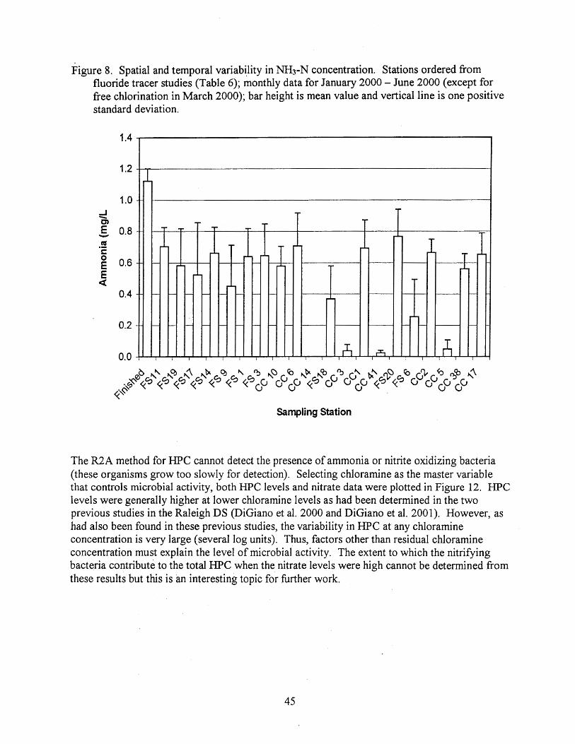
Figure 8. Spatial and temporal variability in NH3-N concentration. Stations ordered from fluoride tracer studies (Table 6); monthly data for January 2000 - June 2000 (except for free chlorination in March 2000); bar height is mean value and vertical line is one positive standard deviation.

1.4

Sampling Station

The R2A method for HPC cannot detect the presence of ammonia or nitrite oxidizing bacteria (these organisms grow too slowly for detection). Selecting chloramine as the master variable that controls microbial activity, both HPC levels and nitrate data were plotted in Figure 12. HPC levels were generally higher at lower chloramine levels as had been determined in the two previous studies in the Raleigh DS (DiGiano et al. 2000 and DiGiano et al. 2001). However, as had also been found in these previous studies, the variability in HPC at any chloramine concentration is very large (several log units). Thus, factors other than residual chloramine concentration must explain the level of microbial activity. The extent to which the nitrifying bacteria contribute to the total HPC when the nitrate levels were high cannot be determined from these results but this is an interesting topic for further work.

Figure 9. Spatial and temporal variability in N03--N concentration. Stations ordered fi-om fluoride tracer studies (Table 6); monthly data for January 2000 - June 2000 (except for free chlorination in March 2000); bar height is mean value and vertical line is one positive standard deviation.

Sampling Station

Figure 10. Evidence of nitrification by increase in NO3--N concentration at two stations (CC3 and FS6) (July 1999 - June 2000)

Figure 11. Evidence of nitrification by increase in NO3--N and decrease in NH3-N concentrations at low chloramine residual (July 1999 - June 2000, exclusive of March 2000 during switch to chlorine)

o Nitrate

Ammonia

Chloramine (mglL)

The nitrate and ammonia concentrations in the DS are shown with pH as the master variable in Figures 13 and 14, respectively. There is a trend toward increasing nitrate and decreasing ammonia with decreasing pH. As Equation 1 indicates, nitrification would be expected to decrease pH for low alkalinity water such as in Raleigh (see Table 7). A wide range of pH was sometimes observed on a given sampling date. The greatest range was found in December 1999 when pH at CC41, CC3 and FS6 was very low (6.7, 7.1 and 7.2, respectively) while very high pH values (9.0 and 9.3) were recorded at two other sampling locations. Poorly buffered water, as is typical of low alkalinity waters in this region of N.C., may be responsible for pH that either decreases or increases within the distribution system. For instance, iron corrosion reactions would lower pH while reactions on cement-lined pipe would increase pH.

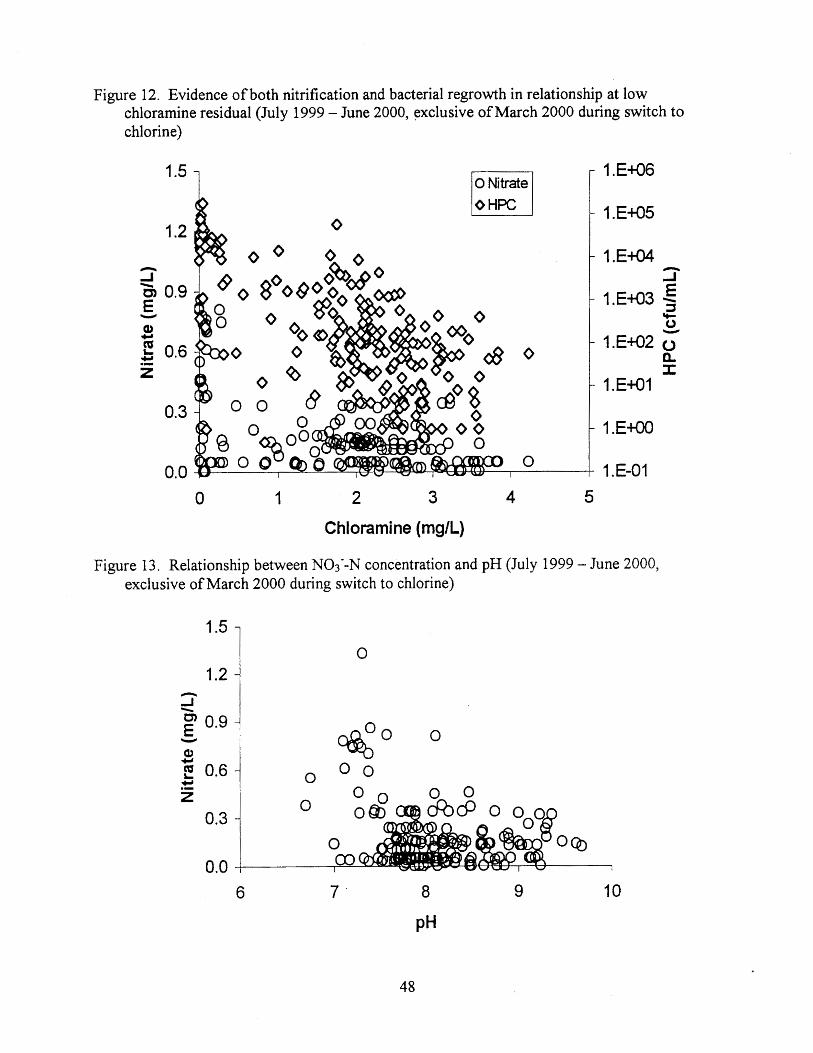
Figure 12. Evidence of both nitrification and bacterial regrowth in relationship at low chloramine residual (July 1999 - June 2000, exclusive of March 2000 during switch to chlorine)

1.5 1 0 Nitrate

Iowc I

0 I 2 3 4 5

Chloramine (mglL)

Figure 13. Relationship between NO+N concentration and pH (July 1999 - June 2000, exclusive of March 2000 during switch to chlorine)

Figure 14. Relationship between m - N concentration and pH

pH Variabilitv in DS

The reasons for the wide range in pH, and particularly the very high values of pH compared to finished water that were noted at some stations, are not understood. In January 2000, a comparison was made of pH measured at the sampling stations by E. M. Johnson WTP staff'with those measured at UNC by graduate research assistants upon return of the samples to the laboratory. The UNC measurements were from 0.3 to 0.6 pH units lower than the site measurements. From February 2000 to June 2000, pH was measured both at the sampling stations and at the UNC laboratory. Both measurements for each sampling station (averaged over the sampling dates) are depicted in Figure 15. The fact that the average pH measured at UNC was lower than measured at some but not all stations does not suggest a consistent measurement difference. More important is the fact that by either measurement, pH values at some stations with long residence time have notably higher pH than stations with relatively short residence times. Keeping in mind that the raw water supply is very low in alkalinity, there is little buffering capacity. Hence, reactions involving iron corrosion products on pipe surfaces and autodecomposition of chloramine could lower the pH greatly while reactions involving cement- line surfaces could increase the pH. Examining pH trends with residence time may not capture the importance of pipe materials.

Wide variations in pH were evident when either free chlorine (March only) or chloramine was used as shown in Figure 16. This is more evidence that wall reactions with poorly buffered water can lead to both a decrease or an increase in pH at various locations in the distribution system.

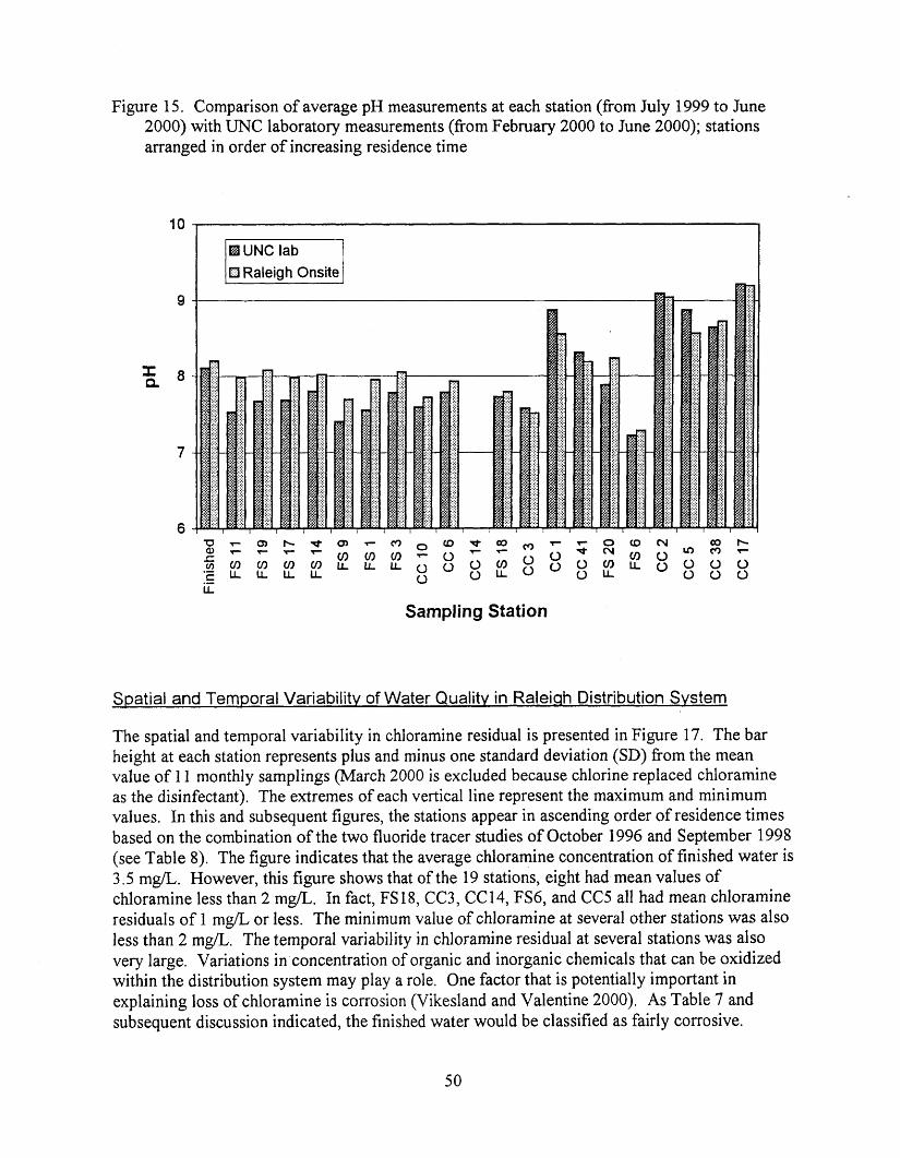
Figure 15. Comparison of average pH measurements at each station (fiom July 1999 to June 2000) with UNC laboratory measurements (from February 2000 to June 2000); stations arranged in order of increasing residence time

I I Raleigh Onsite I

Sampling Station

Spatial and Temporal Variabilitv of Water Quality in Raleigh Distribution System

The spatial and temporal variability in chloramine residual is presented in Figure 17. The bar height at each station represents plus and minus one standard deviation (SD) from the mean value of 11 monthly samplings (March 2000 is excluded because chlorine replaced chloramine as the disinfectant). The extremes of each vertical line represent the maximum and minimum values. In this and subsequent figures, the stations appear in ascending order of residence times based on the combination of the two fluoride tracer studies of October 1996 and September 1998 (see Table 8). The figure indicates that the average chloramine concentration of finished water is 3.5 m&. However, this figure shows that of the 19 stations, eight had mean values of chloramine less than 2 mgL. In fact, FS 18, CC3, CC 14, FS6, and CC5 all had mean chloramine residuals of 1 mg/L or less. The minimum value of chloramine at several other stations was also less than 2 m a . The temporal variability in chloramine residual at several stations was also very large. Variations in concentration of organic and inorganic chemicals that can be oxidized within the distribution system may play a role. One factor that is potentially important in explaining loss of chloramine is corrosion (Vikesland and Valentine 2000). As Table 7 and subsequent discussion indicated, the finished water would be classified as fairly corrosive.

Figure 16. Variation in pH (from July 1999 to June 2000) for use of either fi-ee- or combined chlorine

o Chloramine (7199-6-00) 0

Free Ch lorine (3100) 0 o

0

Figure 17. Spatial and temporal variability of chloramine residual in the DS (July 1999 - June - 2000, exclusive of March 2000 during switch to chlorine))

5

MAX

LL

Sampling Station (in the order of water residence time)

These results are very similar to those reported in previous study of the Raleigh DS (DiGiano et al. 2001) with the original 10 stations (all FS designation). The occurrence of chloramine residuals below 2 mg/L, both spatially and temporally, is cause for concern. North Carolina regulations (Section .2000 - Filtration and Disinfection, .2002 Disinfection) require that the residual disinfectant shall not be less than 2.0 mgL as combined chlorine in more than five percent of the samples each month.

Chloramine demand in the absence of interactions with pipe material was not measured in this study. However, monthly demand data for bulk water samples removed from the distribution system at 10 sampling stations are available for the period of October 1998 to August 1999 (a two-month overlap with current project period) for the previous project (see Table 14 and Figure 32 in DiGiano et al. 200 1). The mean and standard deviation of 48-hour demand were 0.4 and 0.2 m a , respectively. Inspection of Figure 17 shows that the loss in chloramine from the finished water is far greater than the mean plus one standard deviation (0.6 m a ) of previous measurements of bulk water demand for those stations (FS 11 - CC10) with estimated residence times of about 48 hours or less (see Table 8). Given that 10 of the 12 measurements for bulk water demand were taken in months prior to this study and that the residence times are only estimates from one tracer study, firm conclusions are not possible. Nevertheless, the data suggest that chlorarnine demand exceeds that of the bulk water, indicative of the importance of wall reactions. Estimates of a first-order chloramine decay rate at several stations are also available from bulk water measurements taken after 48, 96 and 144 hours on July 20, 1999 (see Figure 3 1 of DiGiano et al. 2001). Using the maximum first-order decay rate of 0.0038 h-', approximately 40% of the chloramine concentration would be lost in 144 hours. With a mean chloramine in the finished water of 3.5 mg/L, the corresponding residual chloramine after 144 hours would be about 2.1 m g L Several stations with residence time in this range (e.g., FS18, CC3, and CC41) had much lower mean value of chloramine residual, again suggestive of loss due to wall reactions.

The spatial and temporal variability of TOC is shown in Figure 18. As was noted in previous studies (DiGiano et al. 2000 and DiGiano et al. 2001), TOC in the finished water remained was fairly constant at about 2.5 mgL and did not decrease with increasing system residence time. Given that the BDOC5 in the finished water is only a small fraction of TOC (about 0.5 mg/L), the loss in TOC is not large enough to measure accurately unless microbial activity was large enough to account for substantial loss of the biodegradable fiaction of TOC.

The spatial and temporal variability in BDOCs are indicated in Figure 19. Stations with BDOCs lower than the finished water would suggest locations where microbial activity has resulted in measurable reduction in substrate concentration. Because data for all sampling dates are grouped together, it is not possible to isolate the spatial change in BDOCs on each sampling date. However, the results showed that the mean value of BDOCs was significantly lower at CCl 0, CC3, CCl, CC41, FS6, CC2, and CC5 than in the finished water. These stations were characterized as having relatively long residence times although the two stations with the longest residence time (CC38 and CC17) were notable exceptions in that the mean BDOCs was no lower than in the finished water. The mean BDOCs at a few stations with relative short residence time

Figure 18. Spatial and temporal variability of TOC concentration in the DS (July 1999 - June 2000)

4 MAX

-

L L


Figure 19. Spatial and temporal variability of BDOCs concentration in the DS (July 1999 - June 2000)


was higher than the mean BDOCj of the finished water. It is difficult to conclude whether this difference is caused by an increase in biodegradable substrate or the imprecision of the BDOCj test.

The spatial and temporal variability of HPC (R2A-PP method) is presented in Figure 20. Mean values of HPC range over a three-log scale (from 10 to lo4 CFUImL). This range is similar to the previous two studies in Raleigh (DiGiano et al. 2000 and DiGiano et al. 2001).

HPC measured at fire station sampling sites was least variable at FS14, with an nearly a two-log difference between the yearly minimum and maximum. This site also had the smallest change in HPC (close to 2-log) between consecutive months. The greatest variability in HPC was found at FS6, with over a 4-log difference between the yearly minimum and maximum. This station also showed the largest difference (over 4-log change) between consecutive months. Higher HPC and greater variability in HPC was measured at the community center sampling sites. The community center with the highest variability was CC41 where there was over 5-log difference between the minimum and maximum monthly values. Likewise, there was over a 5- log change at CC41 between consecutive months. The site showing the least variability in HPC was CClO, with a 3-log difference between the yearly minimum and maximum. Site CClO also had the lowest change in HPC (3-log) between consecutive months.

Figure 20. Spatial and temporal variability of HPC QUA-PP method) in the DS (July 1999 - June 2000)

u,


A large temporal variability could reflect the interaction of a number of time-dependent variables including chloramine residual and BDOC5. Stations with low chloramine residuals (see Figure 17) were also those with the highest HPC value while those with the highest chloramine residuals produced the lowest HET values as expected. Figure 17 also indicates a moderate trend toward higher HPC at longer residence times, although these are only estimates of residence times based on one tracer study. The relationship between HPC and chloramine residual is explored in more detail later (see Figure 22).

Total coliforms were detected by the E. M. Johnson WTP laboratory on three of the 12 monthly samplings. These occurrences are listed in Table 9. Whether fecal coliforms were present cannot be determined from the total coliform test. Both FS6 and CC41 are stations with relatively high HPC and very low chloramine residuals. In the previous 12 months, no positive total coliforms were reported (DiGiano et al. 2001) for the original 10 stations, of which FS6 is included. The high HPC levels and positive coliform occurrences at stations with low chloramine residuals indicate that action is needed to correct these problems. In addition, high HPC are generally known to interfere in the total coliform test. Thus, the absence of total coliform on other sampling dates could be an artifact.

Table 9. Occurrences of Positive Total Coliform

Date Location Comments 212 1/2000 FS6 4/24/2000 FS6 5/24/2000 FS6 Absence after resampling on 5/28/00 5/24/2000 CC4 1

Previous reports (DiGiano et al. 2000 and DiGiano et al. 2001) have included comparison of HPC levels for the months of February (before the N.C. mandated switch from chloramination to free chlorination), March (during free chlorination), April (return to chloramination). Very similar results were obtained during this project period. A summary comparison of HPC data for the three monthly results for all three-project periods covering 1998 through 2000 is provided in Figure 21 (only the 10 original stations in the DS are included). A total of four samples during free chlorination (March) are included for the three-year period. The mean value of HPC in the finished water during March samplings appears rather high due to the detection of one high HPC value (4 100 cfu/mL) on 3/28/2000.

The results indicate that at some stations, the switch to free chlorination produced as much an order of magnitude decrease in HPC levels in the bulk water but the effect was short lived: HPC levels in April generally returned to the values observed in February. To draw firm conclusions about the effect of a change in one parameter (i.e., the switch from chloramine to free chlorine), would require that no other important parameter changed during the month of March. Neither BDOC5 nor temperature was very different in March than in either February or April. It should also be noted that HPC is measured in the bulk water. The switch from chloramine to chlorine may have inactivated biofilm bacteria but this effect cannot be assessed from these data. Other research (Neden et al. 1992 and LeChevalier et al. 1990) has suggested that chloramine is more effective than chlorine in controlling attached bacteria.

Figure 2 1. Comparison of HPC levels before the switch to free chlorine (February), during the switch to free chlorine (March) and after the return to chloramine (April) for 1998, 1999, and 2000

/ February (Chloramine) I El March (free chlorine)

I

The intended purpose of the switch to chlorination is often stated as for control of nitrifying bacteria. In a previous project (DiGiano et al. 2000), nitrification was evident April, May and June, suggesting that chlorination was not effective in prevention of subsequent nitrification. In this project, an increase in nitrate concentrations was taken as evidence of nitrification (see Figures 9 and 10). These data suggest nitrification occurred at two stations in February but not in March. This may indicate that chlorine had suppressed the activity of the nitrifiers but not necessarily inactivated them. Nitrification evidence was also provided again in April but not in May or June. Whether the extent of nitrification upon return to chloramination would have been greater without switching to chlorination is unknown. Controlled laboratory pipe loop experiments would be needed to compare the two strategies.

Figure 22 shows a negative relationship between log HPC and chloramine residual as should be expected. While the scatter is fairly large, as has been observed in both previous studies (DiGiano et al. 2000 and DiGiano et al. 2001), the R~ value is still moderately high (0.38). The R~ value was somewhat higher (0.47) in the second project period (DiGiano et al. 2001) and regression equation was similar.

The correlation between log HPC and BDOCs is presented in Figure 23. The result was a very weak, negative relationship ( R ~ = 0.1 5) but stronger than during the last project ( R ~ = 0.024) (DiGiano et al. 2001). Lower BDOCs may be expected at stations with higher HPCs because substrate has been biodegraded to produce these bacteria. However, the lack of precision of the BDOCs measurement at these low values prevents reaching definitive conclusions.

Figure 22. Relationship between log (HPC) and chloramine residual in the DS (July 1999 - June 2000, exclusive of March 2000 during switch to chlorine)

-1 I I 1 I I 1

0 1 2 3 4 5

Chloramine (mglL)

Figure 23. Relationship between log @PC) and BDOCs in the DS (July 1999 - June 2000)

The relationship of chloramine residual to BDOC:, consumption was tested in Figure 24. BDOC5 consumption was calculated by subtracting the BDOC at each station from the BDOCJ of the finished water. The figure shows that stations with the BDOC5 consumption associated with any chloramine residual varied widely. Given that microbial activity is generally lower at high chloramine residuals (see Figure 22), it was expected that stations with this characteristic would be associated with very little BDOCj consumption while those with low chloramine residual would be associated with very high BDOC5 consumption. Failure to observe this pattern suggests once again the difficulty in interpreting the BDOCJ data.

Figure 24. Relationship between chloramine residual and BDOCj consumption in the DS (data only available for August - December 1999, February 2000 and June 2000); finished water and station FS 14 are not included.

- 4 .O -0.5 0.0 0.5 I .O 1.5

BDOC Consumption (mglL)

Improvement in Water Qualitv at FS6

In late July 2000 at the conclusion of monthly sampling in this project, the City of Raleigh shortened the water residence time at FS6 by installing a 2-inch bypass valve connecting the 495-fl pressure zone to the 595-ft pressure zone. The increase in chloramine concentration and decrease in HPC, as determined by the pour plate method, are shown in Figure 25. Chloramine residual increased fiom 0.07 mgL on July 24 to 1.89 mg/L on August 2. As a result, the HPC decreased fiom 23,000 to 930 CNImL. Based on the findings of this and previous studies (DiGiano et al. 2000 and DiGiano et al. 2001), the action by the City of Raleigh is commendable and also illustrates the practical benefits of cooperative research programs between local governments and universities.

Figure 25. Chloramine concentration and HPC (R2A pour plate) at FS6 for twenty sample dates covering the period before and after the installation of the 2-inch bypass valve near FS6

Identification of Isolates

The results of isolate identification from samples collected on June 26, 2000, and cultured for HPC determinations are presented in Table 10. The Similarity Index is established fiom comparison of the isolate characteristics with those in a database maintained by Analytical Services, Inc, to which these samples were sent. Analytical Services indicates that a Similarity Index of 0.500 or higher with a separation of 0.100 between the first and second choices is generally considered as indicating a good match with the standard. A Similarity Index between 0.300 and 0.500 with a separation of 0.100 between the first and second choices may be a good match. Similarity Indices less than 0.300 indicate that the species is not represented in the database.

The results are difficult to analyze because they represent isolates cultured from samples collected on a single day. The purpose was to isolate as many different morphological types as possible from this single set of samples. No attempt was made to isolate the morphologically most numerous organisms.

The identification with the greatest similarity was for Methylobacterium extorquens as isolated from FS18. This station was characterized by a relatively long residence time (See Table 8) and often had high concentrations of heterotrophic organisms. However, the source of the essential substrate (methanol) for this organism is unknown.

Sphingomonaspaucimobilis is a common soil microorganism. .Hence, its isolation from drinking water is not surprising. This organism could be a member of the attached consortia on pipe walls that can attack poorly degradable compounds in finished water.

Alcaligenes xylosoxydans deniwcans is a denitrifier that has also been reported to be an opportunistic pathogen. This organism could be an inhabitant of the raw water reservoir (Falls Lake). However, its presence in finished water is perplexing because it should have been eliminated by disinfection.

Table 10. Microorganisms isolated and identified in selected samples

Sampling MIDI Organism Identification Similarity Characteristics Site Index

CC2

CC5 CC3 8

CC4 1

FS6 FS9 FS18

Finished Water

Sphingomonas paucimobilis

No identification Sphingomonas paucimobilis

Micrococcus lylae or

Arthrobacter atrocyaneus or

A. aurescens or

Bacillus megatherium GC subgroup B No identification No identification Methylobacterium extorquens or Rhodobacter capsulatus Alcaligenes rylosoxydans denimcans or A. xylosoxydans or A. piechaudii or Kingelia kingae or Yersinia ~seudotuberculosis

Soil bacteria, used in bioremediation. Degrades PAHs and herbicides

Soil bacteria, used in bioremediation. Degrades PAHs and herbicides

Al kanotrophic microbe. Isolated from human skin. Initiates the pathway for degradation of glyp hosphate

Metabolizes methanol. Produces polyhydroxybutyrate

Denitrifier. Highly drug-resistant. Opportunistic pathogen

Comparison of Microbial Methods

Because various microbial enumeration methods are available to assess bacterial regrowth, this phase of the project was aimed at providing a direct comparison. Station FS6 was initially chosen because of its long water residence time (>400 hours) and its history of high HPC (DiGiano et al. 2000 and DiGiano et al. 2001). In this study, monthly samples from July 1999 to

June 2000 had an average HPC (R2A method) of 17,OQO CFUImL and an average chloramine concentration of 0.1 mgL. A site with high HPC was needed in order to obtain at least 30 colonies per plate (required for accurate enumeration) with each of the enumeration methods. However, as noted in an earlier section (Improvement in Water Quality at FS6), the water quality at FS6 improved greatly in August. Because of higher chloramine levels, bacterial regrowth was greatly reduced. With this decreased concentration of bacteria, TGA and PCA spread plates no longer produced 30 or more colonies per plate with the required maximum amount of inoculum (0.1 mL). Because the lower-nutrient R2A media with these incubation conditions grows more bacteria than the TGA and PCA, spread plates with R2A and 0.1 mL of inoculum did give the required 30 or more colonies per plate. Therefore, the PCA and TGA spread plate methods were eliminated from further experiments. However, the PCA and TGA pour plate methods were continued because a 1-mL sample could be used to achieve counts above 30 CFU/mL. These methods were also of particular interest because the Durham water utility uses TGA pour plates whereas the Raleigh laboratory uses PCA pour plates for monitoring HPC.

The pour plate results with the three media for each of 20 sample dates are presented in Figure 26. The R2A-PP were one to three logs higher than on either PCA-PP or TGA-PP. For comparison, the counts for R2A-PP ranged from 220 to 24,000 CN/mL with an average of 5,200 CFU/rnL while those for PCA-PP ranged from 4 to 270 CFUImL, with an average of 72 CFU/rnL and those for TGA-PP ranged fiom 6 to 350 CFUImL with an average of 80 CFU/mL. The difference between the PCA-PP and TGA-PP was not significant. Higher counts were expected from R2A-PP than from either PCA-PP or TGA-PP given past reports from the literature including studies in Durham and Raleigh (DiGiano et al. 2000). While the R2A medium has a lower nutrient content, it is more representative of the natural environment than either the PCA or TGA medium.

The results from R2A-PP, R2A-SP and R2A-MF are compared in Figure 27. No significant difference in results was noted among these methods. HPC from the R2A-PP ranged from 220 to 24,000 CFU/mL with an average of 5,200 CFUImL compared to a range of 270 to 25,000 CFUImL with an average of 5000 CFU/mL for the R2A-SP and a range of 330 to 15,000 CFU/mL with an average of 3000 CFUImL for the R2A-MF.

The results from the AODC method are compared with those from the R2A-PP in Figure 28. The AODC method gave counts ranging fiom 22,000 to 140,000 CFU/mL, with an average of 80,000 CFU/mL. These counts were significantly higher than all of the culturable counts; they were also one to two logs higher than the R2A-PP: This should be expected because the AODC method probably measures all cells (live, dead, and inactive) whereas the culturable count methods measure only those capable of growing under the specific conditions of incubation. After the bypass valve was installed, Figure 27 shows that the AODC increased while the HPC decreased. This could be attributed to an increase in dead or inactive cells.

A box and whisker plot is presented in Figure 29 to show the comparison of all microbial methods. The upper- and lower dashed lines are the maximum minimum values measured for each method. The upper bound of the box is the 75" percentile of all values and the lower bound is the 2 5 ~ percentile of all values for each method. The horizontal line within each box is the mean value. The PCA-PP and TGA-PP gave the lowest values compared to the AODC method.

Figure 26. Comparison of PCA-PP, TGA-PP, and R2A-PP Results at FS6 (May 2000-October 2000)

PCA-PP TGA-PP R2A-PP

100,000 bypass valve was installed

a m a g o C!Q!C!o,x a o a 3 a o 03

Date

Figure 27. Comparison of R2A-PP, R2A-SP, and R2A-MF results at FS6 (May 2000-October 2000)

bypass valve /was installed

( D a m m 7 v- Q Q Q ? i 5 i 5 o o a o 0 0

Date

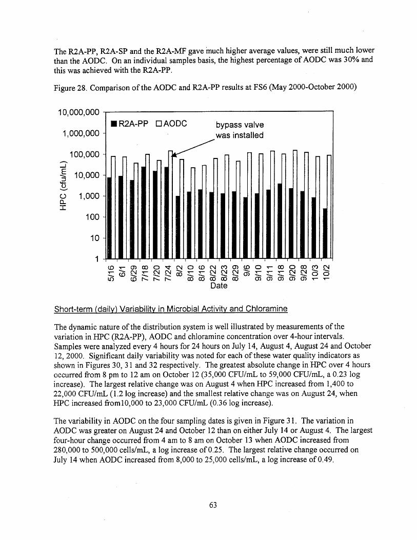
The R2A-PP, R2A-SP and the R2A-MF gave much higher average values, were still much lower than the AODC. On an individual samples basis, the highest percentage of AODC was 30% and this was achieved with the R2A-PP.

Figure 28. Comparison of the AODC and R2A-PP results at FS6 (May 2000-October 2000)

bypass valve was installed

Date

Short-term (daily) Variability in Microbial Activity and Chloramine

The dynamic nature of the distribution system is well illustrated by measurements of the variation in HPC (R2A-PP), AODC and chloramine concentration over 4-hour intervals. Samples were analyzed every 4 hours for 24 hours on July 14, August 4, August 24 and October 12, 2000. Significant daily variability was noted for each of these water quality indicators as shown in Figures 30, 3 1 and 32 respectively. The greatest absolute change in HPC over 4 hours occurred from 8 pm to 12 am on October 12 (35,000 CFU/mL to 59,000 CFU/rriL, a 0.23 log increase). The largest relative change was on August 4 when HPC increased fiom 1,400 to 22,000 CFU/rnL (1.2 log increase) and the smallest relative change was on August 24, when HPC increased fi-om 10,000 to 23,000 CFU/mL (0.3 6 log increase).

The variability in AODC on the four sampling dates is given in Figure 3 1. The variation in AODC was greater on August 24 and October 12 than on either July 14 or August 4. The largest four-hour change occurred fiom 4 am to 8 am on October 13 when AODC increased from 280,000 to 500,000 cells/rnL, a log increase of 0.25, The largest relative change occurred on July 14 when AODC increased from 8,000 to 25,000 cells/mL, a log increase of 0.49.

Figure 29. Box and whisker plot to compare microbial methods for samples taken at FS6 (May 2000 to October 2000).

PCA-PP TGA-PP

A D O C (cellslm L)

Figure 30. Daily variability in HPC (R2A pour technique) at FS 18 on four sampling dates

Time

Figure 3 1. Daily variability in AODC at FS 18 on four sampling dates

Figure 32. Daily variability in chloramine concentration at FS18 on four sampling dates

The variability in chlorarnine concentration on same four sampling dates is shown in Figure 32. Not only is the daily variation important, but also the variation from day to day. Most notably, the chloramine concentration was much higher on July 14 than the other three sampling dates. The effect on regrowth is evident from reinspection of Figures 30 and 3 1; bacterial counts by both HPC and AODC were substantially lower on July 14 than the other three sampling dates. Chloramine concentration changed by as much as 1.28 mg/L in a four-hour period (from 1.80 mg/L at noon to 0.52 mg/L at 4 pm on July 14). The largest relative change occurred on October 12-13, when chloramine increased by a factor of 9 (from 0.2 mg/L to 0.82 mg/L). Changes in chloramine concentration can be caused by variations in water demand and management of storage tank levels that control the reaction time for chloramine demand to be exerted. The fact that the pattern of change is different on different days points to the dynamic nature of distribution systems.

Comparisons of Important Water Quality Relationships Over Three Proiect Periods

The sample collection program for the 10 original stations covered 15 months in the first project period, 11 months in the second project period and 12 months in the third project period. Of this total of 38 months, chloramination was used for 34 months. The relationships between log HPC and chloramine residual for each project period are depicted by different symbols in Figure 33.

The results indicate that a wide range of chloramine residuals was observed in each of the three project periods and these produced a correspondingly wide range of HPC levels. All the data were pooled together to produce the simple regression model given in Figure 34. The R~ value is 0.41 compared to 0.38 when only the third project period data were included. While not strong, the correlation may be useful as a general guide for expectation of HPC levels as measured by the R2A agar method. It is recognized that factors other then chloramine concentration can determine the HPC level. However, our previous project (DiGiano et al. 2000) showed that it was not possible to improve the correlation by including AOC and temperature. AOC is a surrogate for the substrate supply and temperature would reflect seasonal variability that in turn determines the inactivation efficiency of chloramine and the growth rate of bacteria. A non- linear regression model showed that including both temperature and AOC only increased the Pearson correlation coefficient from 0.43 to 0.47.

The importance of both spatial and temporal variability in HPC was analyzed by selecting again pooling data from the three project periods and selecting three stations that were characterized by the fluoride tracer test as having short (8 hr), medium (52 hr) and long residence times (>400 hr). The results are presented in Figure 35. In general, the HPC levels follow the same temporal pattern for each station. There is some evidence for a cyclical pattern of HPC with high values in mid- to late summer and low values in mid-winter that would correspond to temperature effects. A lS°C increase in temperature from winter to summer months produced about a 1-log increase in HPC from winter to summer as shown in the earlier project as well (DiGiano et al. 2001). If growth rate is approximated as first-order, a doubling in rate constant (2kT) accounts for nearly a 1-log increase in bacterial numbers (N) for a 10°C increase in temperature, T [i.e., NT+ldNT = exp (2xkT)/exp (kT); log (NT+lO/NT)~ 7.41. This is a simplistic approach, of course, because the increase in rate of many other processes with temperature affects the HPC.

Figure 33. Relationship between log (HPC) and chloramine residual in the DS for the data for all three projects (March 1997 to June 2000) (free chlorine months are not included)

0 Project #I (3197-5198)

0 Project #2 (1 0198-6199)

A Project #3 (7199-6100)

1 2 3 4

Chloramine (rnglL)

Figure 34. Regression analysis of log P C ) with chloramine residual in the DS after pooling the data from all three project periods (March 1997 to June 2000)

0 1 2 3 4 5 6

Chloramine (mglL)

Figure 35. Variation of HPC at three sampling stations in the DS during all three projects with exception of free chlorination months (March 1997 to June 2000)

D- J- M- M- J- S- N- J- M- M- J- S- N- J- M- M- J- S- N- J- M- M- J- S- 96 97 97 97 97 97 97 98 98 98 98 98 98 99 99 99 99 99 99 00 00 00 00 00

Sampling Date

6

5 - -+- FS 11 (8 hours) + FS 3 (52 hours) -A- FS 6 (394 hours)

RESULTS OF EPANET MODELING

CONVERSION OF EXISTING NETWORK MODEL TO EPANET

The existing network model in WaterMax format was converted into a format compatible with EPANET version 2 (Rossman 2000). Although available only in Beta version at the time of this research, it had been used extensively in the modeling community and its performance and reliability have been documented. The conversion fiorn WaterMax to EPANET was done primarily because EPANET software is available from the US EPA at no cost while WaterMax is proprietary software. Although WaterMax includes a water quality algorithm in its Windows version, the City of Raleigh opted not to purchase the Windows version or the water quality algorithm.

EPANET CALIBRATION PROCEDURE

The pipe network included in the WaterMax model and the location of 12 sampling stations that were used for comparison of MCRT with water age are shown in Figure 36. Also shown are the storage tanks (see Figure 2 for more details on these). Data were entered into EPANET for network components, system operations and wholesale demand for September 2 1, 1998. This day was selected because it coincided with the beginning date of the fluoride tracer study that will be used for MCRT calculations. The City of Raleigh had conducted this tracer study completely independent of our research project and preceding it by nearly one year. The water demand on this date was about 50 MGD, which is almost 20% above the average daily demand for all of 1998 (42 MGD). Pitometer Associates provided the properties of network components that were then converted from a format compatible with the WaterMax model to a format compatible with EPANET 2. Details are provided by Travaglia (2000). Historical data about system operation (pump run time and storage tank levels) were supplied by staff at the E.M. Johnson WTP. Records of daily demand for wholesale users were available at the Public Utilities Department and these are given in Table 1 1 . The EPANET solver used the information collected in the dataset to run dynamic simulations of 24-hour cycles.

The calibration procedure consisted of adjusting some of the parameters in the dataset until the water level in each storage tank of the distribution system predicted by the model matched the level observed on September 21, 1998. Roughness coefficients in pipes and distribution of demand among nodes of a network are the primary parameters typically adjusted in the calibration process. However, the values of the roughness coefficients were not changed in the Raleigh network model from those in the original WaterMax configuration because new field data for pressures and velocities were not available. Furthermore, given the unavailability of billing records and land use maps, the "small retail" water demand (i.e., the average demand for commercial and residential use smaller than 0.1 MGD) was equally distributed among the nodes of the network within each pressure zone. This is a simplistic approach. A more realistic approach would have been to examine building permits issued between 1990 and 1997 and then to adjust the demand upward to reflect changes from 1997 to 1998 using factors applied equally to all nodes in a pressure zone. Whether this approach would have led to better predictions of the system conditions for the September 1998 (pressure and velocity in the pipes, water level

fluctuations in the tanks, etc.) cannot be stated conclusively without considering the importance of large demands by eight wholesale customers. The key data that were missing for these customers were the daily patterns of demand. As will be explained, the experimentation with time patterns of wholesale customer as well as small retail demand was essential to the calibration effort.

Two other adjustments in the input dataset were needed before selecting the final calibration process. During the initial calibration procedure, it was noted that the pump curves in the WaterMax file for three of the pumps at the E.M. Johnson WTP gave different flow rates than measured by the flow meters at the plant. These parameters were adjusted as follows to represent more closely the conditions observed in the Raleigh distribution system. The characteristic curves of pumps 1 and 2 at the Low Service Station and of pump 2 at the High Service Station were moditied to generate the same flow rates measured by the flow meters in the distribution system. The pump characteristics in the Raleigh distribution system, after these adjustments, are listed in Table 12.

The diameter of the Bain storage tank was also changed £tom the WaterMax file value of 320 ft to 277 ft. During the first calibration attempts, it was discovered that the diameter indicated in the Watermax model did not allow reproducing the actual behavior of the distribution system. This conclusion was reached from a flow balance for the Bain system. Although the Bain storage tank is actually three clearwells in series, these were reconsidered as a single, cylindrical tank of a diameter that could be calculated. A time period was selected in which the fill valve replenishing Bain fiom level 495 was closed and the Bain pumps were operating; during this period of time the Bain storage tank drained because it was supplying water to level 495. From the initial and final value of total head (i.e., water level) of the Bain storage tank between 00:OO a.m. to 6:00 a.m., the outflow discharged to the 495 level by the Bain storage tank was calculated from:

where is the net outflow discharged by the storage tank (MG) at time step i in pressure

zone j (MGD); d is the diameter of the storage tank (f12); Ah is the variation in water level (positive if the storage tank empties) which occurred during the 1-hour period between two consecutive telemetric measurements (ft); and K is the factor of 179.50 10' to convert fiom fI3/hr to MGD. The flow rate calculated with Equation 15 was then set equal to the flow rate delivered by the Bain pump to level 495 and the tank diameter was calculated. This method was applied for two different periods of time and the diameter was found to be 277 ft for both.

Figure 36. Pump stations and storage tanks in Raleigh distribution system

Diameter tin1

Sam~lina Stations

I Optimist 2 Millbrook 3 Green 4 Lions Park 5 Halifax 6 Jaycee 7 Pullen 8 Walnut 9 Chavis Park 10 Ralph Campbell I1 Southgate 12 Laurel Hills

Table 1 1. Actual meter readings for wholesale customers

Wholesale Customers Daily Consumption in MGD for 09/21/1998 (fiom Actual Meter Readings)

c W 4.08 (two nodes) Garner 2.42 (two nodes) Knightdale 1.67 Wake Forest 0.6 NCSU 0.9 Aijnomoto 0.45 Wake Medical Center 0.37 Dept. of Correction 0.22

Bain

Pullen Park

Wade

E. M. Johnson WTP - High Service North Hills

Table 12. Hydraulic information for pump stations

Pump To From Pump Rated Total Station Level Level ID Capacity Dynamic

(MGD) Head (ft) E.M. Johnson 495 400 1 12 120 WTP - LOW 2 12 120 Service 3 20 120

4 20 120 5 50 180

495 252 1 4 270 2 3.5 315

595 495 1 1.5 250 2 8 215

595 495 1 9 110 2 14 110 3 27 180

605 495 1 3 240 2 5 210

605 495 1 3 140 2 8 150 3 8 150

Shelley 605 495 1 2.5 160 2 5 180

Leesville 655 605 1 1 60 2 1 60

INPUT DATA: SYSTEM OPERATIONS

Pump and fill-valve status (ordoff) and tank water levels were available at the E. M. Johnson WTP in the form of SCADA printouts. The variation of water level in the storage tanks for September 21-25, 1998, within each pressure zone was not strongly cyclical as may be expected by typical variations in demand throughout each day (Travaglia 2000). The elevated storage tanks (Springfield, Leesville, Strickland, Six Forks, Fairground and Highway 54) with a capacity of 1 MG or less showed the greatest departure from this pattern. These storage tanks finction as pressurizing facilities, in addition to providing water supply during peak demand. Conversely, the North Hills and Bain storage tanks (that do not flow on any of the pressure zones) showed more periodicity in daily water level fluctuations than the other storage tanks. The fill-valves that regulate the inflow to these two tanks are always operated in the same manner. They are usually left open at night to fill these tanks when demand in the system is low, while they are generally closed during the day when the tanks supply the 495 and 605 levels.

The data provided from the E. M. Johnson WTP indicated that a simple set of rules to determine when to turn the pumps on and off was not in place. In most municipal water supply facilities, a pump is turned on (or off) when the water in a specified storage tank reaches a minimum (or maximum) level, and operational strategies typically aim to minimize power costs that guarantee acceptable pressures in the system (Cesario 1995). However, the Raleigh operators explained that the pumps are turned on when the rate of drainage for storage tanks is too fast, even when they are still full. The operators look at the monitor of the SCADA system where the total head (ft) of each storage tank is shown in real time. The operators try to keep the water level in the storage tanks close to their maximum value at all times. No other control rule is currently applied to the pumps in the Raleigh network and the pump operation is highly dependent upon the experience of the operator. Maintenance of high water levels would suggest long storage times and thus the opportunity for increased chloramine decay that could lead to bacterial regrowth and nitrification. However, no measurements were made of water quality within storage tanks during this research.

INPUT DATA: WATER DEMAND

The demand generated by wholesale users and large internal customers is referred to as WSD. The total amount of water sold to each wholesale user is measured every day from actual meter readings. On September 21, 1998, the WSD was equal to 10 MGD, as shown by summation of the demands in Table 1 1. This equates to approximately one-fifth of the average daily water production estimated to be 50 MGD from the E.M. Johnson WTP for September 21, 1998. The hourly variations in WSD were not recorded. This was a key piece of data that had to be estimated to run EPANET simulations. The hourly variations in WSD and small retail demand (SRD) on September 21, 1998, were required in order to calibrate the model. An estimate of WSD and SRD variations on the day in which the calibration took place was accomplished through the following steps: (1) predictions of pump flow rates at 30-minute intervals; (2) estimation of total demand at 30- minute intervals; and (3) estimates of WSD and SRD at 30- minute intervals (Travaglia 2000).

INITIAL CALIBRATION EFFORTS

The effectiveness of each assumption made to determine the WSD was verified by running EPANET and comparing the predicted and observed storage tank water levels for September 21, 1998. If the predictions matched the field measurement, the assumptions were accepted; otherwise, they were changed. The first approach used to determine the WSD was to assume that the wholesale users are supplied at a constant flow rate. For example, the WSD would be 4 MGD throughout the day if the meter readings showed 4 MG of water sold for that day. This approach was justified by the fact that, typically, municipalities tend to minimize changes in pump operations in order to reduce energy expenses. If Cary's demand was assumed constant throughout the day, the EPANET predictions showed that the storage tanks at Fairground Rd. and Highway 54 Rd. in the 595 level would be drained at a faster rate than observed. The same results were found for Elevation 495. In this case, the Chamberlin storage tank and the New Hope storage tank were drained at a faster than actual rate because the predicted water demand, which was assumed to be constant from the towns of Knightdale, Gamer and Wake Forest is higher than the actual demand (Travaglia 2000).

FINAL CALIBRATION EFFORT

The discrepancy between the EPANET simulation and the observed tank level data can be attributed to failure to include variable WSD throughout the day. If a variable WSD were to be used, the constraint would be that the total volume of water delivered during the 24-hour period simulation is equal to the average daily consumption obtained from actual meter readings for September 2 1, 1998. Pitometer Associates confirmed that each pump station supplying the wholesale users has multiple pumps with characteristic curves that differ from one another. This feature enables the Raleigh system to deliver water to each wholesale user at different flow rates, for the same levels of pressure, depending on the combinations of pumps operating at that particular moment in time.

The towns of Gamer, Knightdale and Wake Forest, in addition to the two-pump stations at Cary represent the boundary conditions for the Raleigh system and were modeled as nodes with a large demand. In order to obtain a reasonable agreement between predicted and observed performance, the WSD was varied by entering a different demand as a multiplier of the average demand at each time step through a trial and error approach until the predicted and observed water levels in the storage tanks were in agreement. The WSD patterns shown in Figure 37a-c were finally selected. Figure 3 8 shows the corresponding extent of agreement between predicted and observed water levels for the storage tank at Highway 54. The simulation output for the other storage tank water levels in the Raleigh system after completion of the calibration procedure is shown in Figures 39 - 47. The calibration statistics generated by comparing EPANET predictions with field observations (Travaglia 2000) implied that EPANET produced predicted values of storage tank levels with the exception of the Strickland tank that were fairly close to those observed. The agreement was similar when the simulation period was extended from one day to five days to cover the days subsequent to September 21, 1998 for fluoride tracer data were available (Travaglia 2000). However, as in any calibration exercise, the path to achieve the results must be carehlly scrutinized. In particular, the la& of informatjOn

Figure 37. Demand patterns for wholesale users (a) Cary pump station no. 1 (b) Cary pump station no. 2 and (c) Gamer, Knightdale and Wake Forest

Time (hours)

Time (hours)

Time (hours)

Firmre 38. Comaarison of EPANET predictions and field observations for Highway 54 storage U

tank (595 lekel) with assumption of WSD varying with time

8 12 16 20 24

Time (hours)

Figure 39. Comparison of EPANET predictions and field observations for Fairground (595 level) with assumption of WSD varying with time

8 12 16 20 24

Time (hours)

Figure 40. Comparison of EPANET predictions and field observations for Bain (495 level) with -

assumption of WSD varying with time

+- Predicted esl Measured

rn

0 4 8 12 16 20 24

Time (hours)

Figure 41. Comparison of EPANET predictions and field observations for Chamberlin (495 level) with assumption of WSD varying with time

0 4 8 12 16 20 24

Time (hours)

Figure 42. Comparison of EPANET predictions and field observations for North Hills (495 level) with assumption of WSD varying with time

I -t Predicted I I a Measured /

8 12 16

Time (hours)

Figure 43. Comparison of EPANET predictions and field observations for New Hope (495 level) with assumption of WSD varying with time

-+ Predicted Measured

8 12 16

Time (hours)

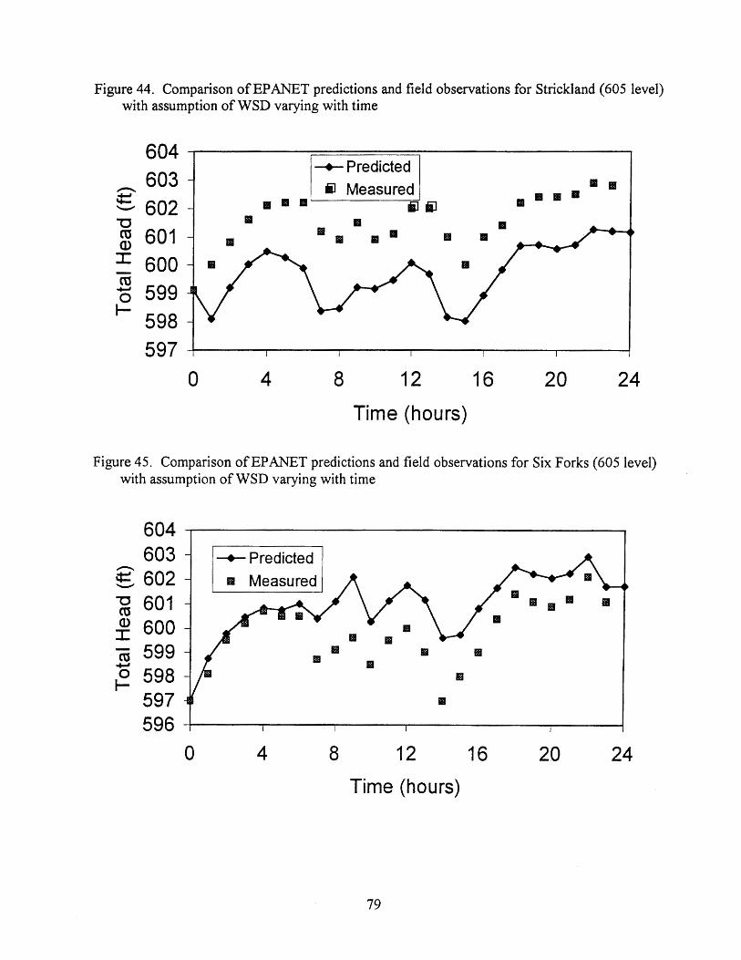
Figure 44. Comparison of EPANET predictions and field observations for Strickland (605 level) with assumption of WSD varying with time

I +- Predicted I / Measured 1

8 12 16

Time (hours)

Figure 45. Comparison of EPANET predictions and field observations for Six Forks (605 level) \

with assumption of WSD varying with time

8 12 16

Time (hours)

Figure 46. Comparison of EPANET predictions and field observations for Leesville (level 655) with assumption of WSD varying with time

Time (hours)

Figure 47. Comparison of EPANET predictions and field observations for Springdale (655 level) with assumption of WSD varying with time

8 12 16

Time (hours)

network components, system operations and demand forced major assumptions including synthesis of characteristic curves of three pumps at the E.M. Johnson WTP, demand allocation and daily variations. For instance, a major assumption was made about the diurnal demand pattern for Garner without much supporting information. A more appropriate way to perform the calibration is recommended, in which the roughness coefficients in the pipes and the demand allocation among the nodes are calibrated fiom the results of a tracer study and new field- measurements of the pressures in the distribution system.

COMPARISON OF WATER AGE AND MCRT

As explained in the Background section (see Equations 10-12), the MCRT is based on the analysis of the fate of fluoride (I?'), a conservative tracer introduced at the WTP and followed throughout the distribution system. Of interest is the comparison between the MCRT and water age as calculated within EPANET because they are two measures of water residence time, each determined by very different means (MCRT by tracer response and water age by hydraulic and water quality simulations). Having an alternative to the modeling of water age would allow water utilities to decide the location of sampling stations where disinfectant residuals may be low or where disinfectant byproducts may be high.

The MCRT calculation was used to interpret results of a F- tracer study that was performed from September 21 to September 25, 1998. The MCRT was then compared to water age as predicted by EPANET after the calibration as described in the previous section.

The MCRT approach assumes that the input of F- into the distribution system is a negative step stimulus, while in reality the actual input is exponential. This is so because F is typically added between the filters and the cleanvell. As a consequence, the mixing conditions in the cleanvell attenuate the F concentration generated at the chemical feeder and the resulting tracer input to the distribution is an exponential rather than step decrease in concentration. This is shown in Figure 48 by the time pattern of F' leaving the clearwell during the tracer test of September 2 1, 1998. The first objective of this work was to test whether a violation in assumption of a negative step input would generate significant differences between the results computed with the MCRT method and EPANET predictions of water age. The test consisted of using EPANET to compare the response to an idealized negative step stimulus with an exponential decrease in F- concentration at the exit point of water from the clearwell into the distribution system. For each of these simulation outputs, the F- concentration-time curves were used to determine the average residence time at selected locations of the network. The results obtained for the two types of F- input were then compared. The second objective was to compare water age as generated from EPANET at selected stations in the distribution system with the MCRT for a specified F tracer stimulus input. The final objective was to compare the predicted MCRT to field-measured MCRT from a 1998 fluoride tracer study to assess the impact of skeletonization of the Raleigh distribution system.

The model was used to simulate a F- tracer study in which the feed at the E. M. Johnson WTP was turned off to produce: (1) a negative step input and (2) an exponential-like decline in F- concentration. The latter input pattern was taken from the actual measurements of F-made at the exit of the clearwell during the 1998 fluoride tracer study (Figure 48). From the simulation

Figure 48. Fluoride tracer pattern at the E.M. Johnson WTP

Time elapsed (days)

output, the comparison between the MCRT for the two types of stimulus, as well as the comparison between MCRT and water age by EPANET, were computed.

Figures 49-51 show the predicted fluoride response for both types of stimulus at three of the sampling station in the Raleigh distribution system. As expected, the fluoride concentration predicted by EPANET reaches the background level somewhat more rapidly for the negative step input than for the actual fluoride input. However, the fluoride tracer response is not significantly affected by the assumption used for the stimulus.

The MCRT at the sampling nodes was determined from each of the tracer response curves using Equation 12. These results are listed in Table 13 and shown in Figure 52 for both the assumptions about the tracer stimulus. The correlation coefficient between the predicted MCRT based on the actual stimulus and the negative step stimulus was 0.93. This reinforces the idea that the simplifying assumption of a negative step stimulus is acceptable.

'

Figure 49. EPANET predictions of tracer response at Millbrook Station for simulations of negative step and actual stimuli at E. M. Johnson WTP

Time (hours) elapsed from the beginning of the experiment

Figure 50. EPANET predictions of tracer response at Optimist Station for simulations of negative step and actual stimuli at E. M. Johnson WTP


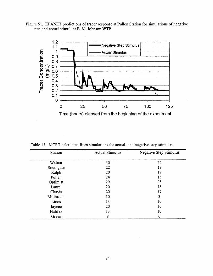
Figure 5 1. EPANET predictions of tracer response at Pullen Station for simulations of negative step and actual stimuli at E. M. Johnson WTP

N e g a t i v e Step Stimulus

-Actual Stimulus


Table 13. MCRT calculated from simulations for actual- and negative-step stimulus

Station Actual Stimulus Negative Step Stimulus

Walnut 30 22 S outhgate 22 19

Ralph 20 19 Pullen 24 15

Optimist 29 25 Laurel 20 18 Chavis 20 17

Millbrook 10 3 Lions 13 10 Jaycee 20 16 Halifax 13 10 Green 8 6

Figure 52. Comparison of MCRT for actual- and negative-step stimulus both from EPANET simulations

Halifax

Millbroo 1 GreenH/

0 5 10 15 20 25 30 Predicted MCRT with Negative Step Stimulus

(hours)

Figure 53 shows the water age predicted by EPANET at one of the sampling stations of the Raleigh network for a 5-day simulation. The influence of water level variations and their residence time in storage tanks is evident. At most sampling nodes, water age reaches a maximum at around 9:00 a.m. when the distribution system has a peak in demand and the storage tanks drain to meet this demand. The water parcels that were held in the storage tanks during the night are released into the network and hence, contribute to increase the age of water in the pipes of the distribution system.

Figure 53. Simulated water age at Southgate Station

Time (hours) elapsed

Figure 54 suggests a satisfactory level of correlation (correlation coefficient equal to 0.94) between the calculated MCRT and the average water age from EPANET. However, as was shown in Figure 53 for one station, the difference between minimum and maximum water age due to fluctuations in water level in storage tanks is noticeable. The MCRT is compared to the maximum and minimum water age in Table 14 and shows that the dynamic variations in water age cannot be captured.

Figure 54. Comparison of average water age and MCRT, both calculated from EPANET

Optimist walnut~/ UJ

t .- w V) Jaycee ?;; 20 - 3 C 0 a 5 1 5 - .- 3 Lions e!

Predicted Water Age (hours)

The agreement between predictions and measurements of fluoride tracer responses observed at each station was quite variable. The fluoride concentration-time curves predicted by EPANET using the actual stimulus and the same curves obtained from field measurements at each sampling station in the Raleigh DS during the 1998 tracer study are included as Appendix ILL Examples are given in Figures 55 and 56. The agreement was fairly good at the Walnut Terrace Station (Figure 55) but very poor at the Southgate Station (Figure 56). The following are possible explanations for lack of agreement: skeletonized model did not match real system; model was out-of-date and thus, not properly re-calibrated for this project for lack of data; valves were improperly specified as open when they were closed and vice versa; the network of pipes supplying the service lines to the sampling stations was not accurately represented in the network model; and assumptions about diurnal demand pattern for wholesale of water to Garner may have be questionable. In general, a skeletonized model will predict shorter water ages and thus a more rapid decrease in fluoride concentration in such tracer studies than would be actually observed. This is because fewer pipes means fewer paths for water to travel and this would lead to higher velocity and shorter water age.

Table 14. Comparison of MCRT from simulation of actual tracer stimulus in EPANET with predictions of average, maximum and minimum water ages

Station MCRT for Average Water Maximum Minimum Actual Tracer Age (hours) Water Age Water Age

Stimulus (hours) (hours) (hours) \ /

Walnut 30 28 75 10 S out hgate 22 23 53 15 Ralph 20 22 47 15 Pullen 24 19 36 8 Optimist 29 26 34 8 Laurel 20 22 62 13 Chavis 20 21 52 12 Millbrook 10 3 4 2 Lions 13 11 13 7 Jaycee 20 18 20 15 Halifax 13 11 13 9 Green 8 3 5 3

Figure 5 5. Predicted versus observed fluoride concentration at Walnut Station


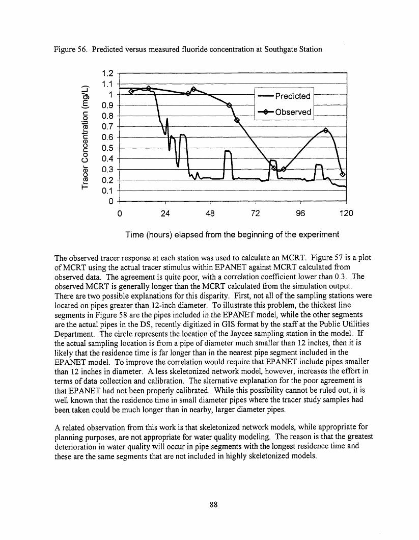
Figure 56. Predicted versus measured fluoride concentration at Southgate Station


The observed tracer response at each station was used to calculate an MCRT. Figure 57 is a plot of MCRT using the actual tracer stimulus within EPANET against MCRT calculated from observed data. The agreement is quite poor, with a correlation coefficient lower than 0.3. The observed MCRT is generally longer than the MCRT calculated from the simulation output. There are two possible explanations for this disparity. First, not all of the sampling stations were located on pipes greater than 12-inch diameter. To illustrate this problem, the thickest line segments in Figure 58 are the pipes included in the EPANET model, while the other segments are the actual pipes in the DS, recently digitized in GIs format by the staff at the Public Utilities Department. The circle represents the location of the Jaycee sampling station in the model. If the actual sampling location is from a pipe of diameter much smaller than 12 inches, then it is likely that the residence time is far longer than in the nearest pipe segment included in the EPANET model. To improve the correlation would require that EPANET include pipes smaller than 12 inches in diameter. A less skeletonized network model, however, increases the effort in terms of data collection and calibration. The alternative explanation for the poor agreement is that EPANET had not been properly calibrated. While this possibility cannot be ruled out, it is well known that the residence time in small diameter pipes where the tracer study samples had been taken could be much longer than in nearby, larger diameter pipes.

A related observation fi-om this work is that skeletonized network models, while appropriate for planning purposes, are not appropriate for water quality modeling. The reason is that the greatest deterioration in water quality will occur in pipe segments with the longest residence time and these are the same segments that are not included in highly skeletonized models.

Figure 57. Comparison of MCRT determined from the simulations and field-measurements

Figure 58. Location of sampling stations in relation to pipes included in Raleigh network model

k a I n u t . O pti mist

Pullen Southgate

Ralph IP

Lions 81

Jaycee

0 10 20 30 40 50 60 70 80

Observed MCRT (hours)

REFERENCES

Alegre, H. and S.T. Coelho. 19%. A methodology for the characterization of water consumption. Integrated Computer Applications in Water Supply, 3 69-3 84. United Kingdom:Research Studies Press Ltd.

Allgeier, S. C., R. S. Summers, J. G. Jacangelo, V. A. Hatcher, D. M. Moll, S. M. Hooper, J. W. Swertfeger, and R. B. Green. 1996. A simplified and rapid method for biodegradable dissolved organic carbon measurement. In proceedings of the Amer. Water Works Assoc. Water Quality Technology Conference, Boston, Mass. (CD-ROM)

American Public Health Association (APHA). 1985. StarrdardMethods for the Examination of Water and Wastewater, 15th ed. Washington, D. C.

American Public Health Association (APHA). 1 998. Standard Methods for the b i n a t i o n of Water and Wastewater, 20th ed. Washington, D. C.

Buchberger, S., G. Wells, and J. Greg. 1996. Intensity, duration, and frequency of residential water demand. Jour. of Water Resources Planning and Management, 122(1): 1 1 - 19.

Cesario, L. 1 995. Modeling analysis, and design of water distribution systems. Denver: Amer. Water Works Assoc.

Clark, R. M. and W. M. Gray man. 1 998. Modeling water quality in drinking water distribution systems. Denver: h e r . Water Works Assoc.

Clark, R. M. and M. Sivaganesan. 1998. Predicting chlorine residuals and formation of TTHMs in drinking water. Jour. Env. Eng. Div., A X E 124(12):1203-1210.

Cruickshank, J. R. 1993. Pitometer water distribution study, Raleigh, North Carolina, Report to the Public Utilities Department, City of Raleigh, N.C.

DiGiano, F. A., D. Francisco, W. Zhang and L. Todd. 2000. Bacterial regrowth in drinking water systems: A comparison of Durham and Raleigh. Report No. 326 of the Water Resources Research Institute of The University of North Carolina, Raleigh, NC.

DiGiano, F. A., W. Zhang, D. Francisco, and M. Wood. 2001. Data collection to support a simplified bacterial regrowth model for distribution systems. Report No. 33 1 of the Water Resources Research Institute of The University of North Carolina, Raleigh, NC.

Engineering Computer Applications Committee. 1999. Calibration guidelines for water distribution system modeling. In Proceedings of Amer. Water Works Assoc. ImTech Conference. Denver: Amer. Water Works Assoc.

Fiksdal, L., E. Vik, A. Mills and J. Staley. 1982. Nonstandard methods for enumerating bacteria in drinking water. Jour. Amer. Water Works Assoc. 74(6):3 13-3 18.

Francisco D. E., Mahand R. A. and Rabin A. C. 1973. Acridine-orange-epifluorescence technique for counting bacteria in natural waters. Trans. Am. Microsc. Soc. 92:4 1 6.

Grayman, W. M. and R. M. Clark. 1993. Using computer models to determine the effect of storage on water quality. Jour. Amer. Water Works Assoc. 85(7): 67-77.

Kennedy, M. S., S. Moegling, S. Sarikelle and K. Suravallop. 1993. Assessing the effects of storage tank design on water quality. Jour. Amer. Water Works Assoc. 85(7): 78-88.

LeChevallier, M. W., C. D. Lowry and R. G. Lee. 1990. Disinfection of biofilms in a model distribution system. Jour. Amer. Water Works Assoc. 82(7):87-99.

Lieu, N. I., R L. Wolfe and E. G. Means III. 1993. Optimizing chloramine disinfection for the control of nitrification. Jour. Amer. Water Works Assoc. 85(2): 84-90.

Lineaweaver, F.P., J. Geyer Jr. and J. B. Wolff. 1967. Summary report on the residential water use research project. Jour. Amer. Water Works Assoc. 59(3):267-282.

McGuire, M. J., N. I. Lieu and M. S. Pearthree. 1999. Using chlorite ion to control nitrification. Jour. Amer. Water Work; Assoc. 9 1 (1 0): 52-6 1.

Means, E., L. Hanami, H. Ridgway and B. Olson. 1981. Evaluating mediums and plating techniques for enumerating bacteria in water distribution systems. Jour. Amer. Water Works Assoc. ( 1 1):585-590.

Neden, D. G., R. J. Jones, J. R. Smith, G. J. Kirmeyer and G. W. Foust. 1992. Comparing chlorination and chloramination for controlling bacterial regrowth. Jour. Amer. Water Works Assoc. 84(7): 80-88.

Norton, C. D. and M. W. LeChevallier. 1997. Chloramination: Its effect on distribution system water quality. Jour. Amer. Water Works Assoc. 89(7):66-77.

Odell, L. H., G. J. Kirkmeyer, A. Wilczak, J. G. Jacangelo, J. P. Marcinko and R. L. Wolfe. 1996. Controlling nitrification in chloraminated systems. Jour. Amer. Water Works Assoc. 88(7): 86-98.

Ormsbee, L. E. and S. Lingireddy. 1997. Calibrating hydraulic network models. Jour. Amer. Water Works Assoc. 89(2): 42-5 0 .

Reasoner, D. J. and E. E. Geldreich. 1985 A new medium for the enumeration and subculture of bacteria from potable water. Appl. & Env. Microbiology 49(1): 1-7.

Reasoner, D. J., J. C. Blannon, E. E. Geldreich and J. Barnick. 1989 Nonphotosynthetic pigmented bacteria in potable water treatment and distribution system. Appl. & Em. Microbiology 55(4):912-921.

Regan, J. M., G. W. Hamngton and D. R. Noguera. 2002. Ammonia- and nitrite-oxidizing bacterial communities in a pilot-scale chloraminated drinking water distribution system. Appl. & Env. Microbiology 68(1):73-8 1.

Reddy, L.S., L. E. Ormsbee Lindell and D. J. Wood. 1995. Time-averaging water quality assessment. Jour. Amer. Water Workr Assoc. 87(7): 64-73.

Rossman, L. A. 1994. EPANET Users Manual. Risk Reduction Engineering Laboratory, USEPA, Cincinnati, Ohio.

Rossman, L.A. and P. F. Boulos. 1993. Discrete volume-element method for network water- quality models. Jour. of Water Resources PlanningandManagement. 119(5):505-5 17.

Rossman, L. A. 2000. Computer models/EPANET. In Water distribution systems handbook, edited by L. Mays. New York: McGraw-Hill.

Rossman, L, A. and P. F. Boulos. 1996. Numerical methods for modeling water quality in distribution systems: A comparison. Jour. of Water Resources Planning and Management. 122(2): 137-146.

Skadsen, J. 1993. Nitrification in a distribution system. Jour. Amer. Water Works Assoc. 85(7):95-103.

Snoeyink, V. L. and D. Jenkins. 1980. Water chemistry. New York: Wiley.

Travaglia, A. 2000. Comparison of mean constituent residence time (MCRT) from fluoride tracer studies and water age from EPANET modeling of distribution systems. Masters Technical Report. Dept. of Environmental Sciences and Engineering, University of North Carolina, Chapel Hill, NC.

U. S. EPA. 1993. Methods for the determination of inorganic substances in environmental samples. EPA/600/R-93-100 (Available as NTIS Report No. PB94-120821).

Vasconcelos, J., L. A. Rossman, W. M. Grayman, P. F. Boulos and R. M. Clark. 1997. Kinetics of chlorine decay. Jour. Amer. Water Works Assoc. 89(7): 55-65.

Vikesland, P., K. Ozekin and R. Valentine. 1998. Effect of natural organic matter on monochloramine decomposition: Pathway elucidation through the use of mass and redox balances. Environ. Sci. Technol. 32(10): 1409- 14 16

Vikesland, P and R. Valentine. 2000. Reaction pathways involved in the reduction of monochloramine by ferrous iron. Environ. Scz. Technol. 34(l): 83 -90.

Walski, T. M. 2000. Modeling calibration cata: The good, the bad and the useless. Jour. Amer. Water Works Assoc. 92(1):94-99.

Weber, W. J., Jr. and F. A. DiGiano. 1996. Process dynamics in environmental ystems (Chapter 9). New York: Wiley Interscience.

Wilczak, A., J. G. Jacangelo, J. P. Marcinko, L. H. Odell, G. J. Kirkmeyer and R. L. Wolfe. 1996. Occurrence of nitrification in chloraminated distribution systems. Jour. Amer. Water Works Assoc. 8 8(7) : 74-8 5.

APPENDIX I. LIST OF SYMBOLS

Ai j cross-sectional area of link ij in distribution system

AOB ammonia oxidizing bacteria

AOC assimilable organic carbon

BDOC5 biodegradable dissolved organic carbon measured after 5 days of sample incubation

Cij concentration of substance in link ij of distribution system

Gi external source concentration entering node i of distribution system

CC community center sampling locations

CFU colony forming units

c12 chlorine

C102- chlorite

DOC dissolved organic carbon

DS distribution system

DVM discrete volume element method

EPS extended period simulation

F 0) fractional composition of "new water" mixing with the water containing the original composition of fluoride (prior to the step input) at a selected location

F, (0 average fractional concentration of fluoride in time interval, I

FS fire station sampling locations

HPC heterotrophic plate count

ki subscript describing a link with flow into the head node i of link ij

LI Larson index

Lki length of link ki

MCL

MCRT

MF

MG

MGD

N

mc1

NJ33

NOB

NOi

No3-

P

PCA

PP

9i

qsi

R(cij)

R2A

SD

S 0 - 4

SP

SRD

t

t1

t*

maximum contaminant level

mean constituent residence time

membrane filtration

million gallons

million gallons per day

nitrogen

monochloramine

ammonia

nitrite oxidizing bacteria

nitrite

nitrate

phosphorus

standard plate count agar

pour plate

constant flow rate in link ij at time t in distribution system

flow rate of an external source

reaction rate expression in link of distribution system

type of agar in HPC determination

standard deviation

sulfate

spread plate

small retail demand

time

time interval, i

mean residence time

TGA

TH

TOC

UNC

WSD

WTP

Xij

tryptone glucose agar used in standard HPC determination

total head

total organic carbon

University of North Carolina

wholesale demand

water treatment plant

distance along link ij in distribution system

APPENDIX 11. FLUORIDE TRACER DATA AT NINE COMMUNITY CENTER

SAMPLING SITES IN 1998 TRACER STUDY

Figure 11.1. Fluoride response curve at CC 10 (Optimist)

40 60 80

Time (hour)

Figure 11.2. Fluoride response curve at CC6 (Jaycee)

CC 6 (Jaycee)

40 60 80

Time (hour)

Figure 11.3. Fluoride response curve at CC3 (Chavis Park)

CC 3 (Chavis Park)

I I I I I

40 60 80 Time (hour)

Figure 11.4. Fluoride response curve at CCI (l3iltmore Hills)

CC 1 (Biltmore Hills)

I I . I I I


Figure 11.5. Fluoride response curve at CC41 (Lake Lynn)

1 CC 41 (Lake Lynn)


Figure 11.6. Fluoride response curve at CC2 (Carolina Pines)


-

-

i-

0.0

CC 2 (Carolina Pines)

I I I I I

Figure 11.7. Fluoride response curve at CC5 (Halifax)

CC 5 (Halifax)


Figure 11.8. Fluoride response curve at CC 17 (Worthdale)

CC 17 (Worthdale)


Figure 11.9. Fluoride response curve at CC38 (Laurel Hills)

CC 38 (Laurel Hills) I I I l I


APPENDIX Ill. COMPARISON OF FLUORIDE CONCENTRATIONS PREDICTED BY

EPANET AND OBSERVED AT EACH SAMPLING STATION IN 1998 TRACER

STUDY

Figure 111.1. Comparison of fluoride concentrations predicted by EPANET and observed at Walnut Station

Figure 111.2


Comparison of fluoride concentrations predicted by EPANET and observed at Southgate Station

1.2 - Predicted

Southgate 0.0 1 I I 1

0 24 48 72 96 120


Figure 111.3. Comparison of fluoride concentrations predicted by EPANET and observed at Ralph Station

Ralph

A. - Predicted

0 24 48 72 96 120


Figure III.4. Comparison of fluoride concentrations predicted by EPANET and observed at Pullen Station

- Predicted

\I -9- Observed

0 24 48 72 96 120


Figure IDS. Comparison of fluoride concentrations predicted by EPANET and observed at Optimist Station

I Optimist

- Predicted


Figure 111.6. Comparison of fluoride concentrations predicted by EPANET and observed at Millbrook Station

0 25 50 75 100 125


Figure II1.7. Comparison of fluoride concentrations predicted by EPANET and observed at Lions Station

- Predicted

-+- Observed


Figure III.8. Comparison of fluoride concentrations predicted by EPANET and observed at Laurel Station

Laurel

- Predicted

-+- Observed

0 24 48 72 96 120


Figure 111.9. Comparison of fluoride concentrations predicted by EPANET and observed at Jaycee Station

- - Predicted

0 25 50 75 I 00


Figure III. 10. Comparison of fluoride concentrations predicted by EPANET and observed Halifax Station

- Predicted

0 25 50 75 1 00 125


0.0 Hal if ax

1 I I I

Figure 111.11. Comparison of fluoride concentrations predicted by EPANET and observed at Green Station

- Predicted -+- 0 bserved

0 25 50 75 100 125


Figure III. 12. Comparison of fluoride concentrations predicted by EPANET and observed at Chavis Station

- Predicted - + /*-* \ -*-Observed

C havis


occurrence of bacterial regrowth and nitrification in …

Documents