ocean circulation and surface buoyancy fluxes: … · ross griffiths! with credits: graham...
TRANSCRIPT

Ross Griffiths!with credits: Graham Hughes, Andy Hogg, !Kial Stewart, Julia Mullarney, J.Tan !
Ocean circulation and surface buoyancy fluxes: dynamics and energetics !
Research School of Earth Sciences The Australian National University!!

• sinking of dense water; distributed upwelling!• vertical mixing maintains stratification!• energy inputs and rates of turbulent mixing?!• mean flow – roles of buoyancy, wind stress and mixing?!
Meridional Overturning Circulation (MOC)!Net Heating Net CoolingNet Cooling Wind Stress Wind Stress
550S!650N!
(q)
00!

• Role of buoyancy?!
The ocean energy budget!
From Wunsch & Ferrari (2004)
~2TW

• Convection under differential surface heating/cooling!• Available Potential Energy (APE) !• Energy pathways in stratified / convecting flows!• A connection between turbulent mixing and buoyancy forcing!• Ocean models and the roles of surface buoyancy (and wind) forcing!
Outline!

• Non-uniform heating/cooling at base; zero net heat input!• narrow end wall plume, broad downward return flow!• stratification relies on interior vertical diffusion!!
Surface buoyancy forcing – Rossbyʼs experiment!
Rossby !(1965, 1998)!
Ra~108!
Temp !gradient!

• Ra ~ 1012 or RaF ~ 1014; flow insensitive to form of BCs!• transitions: small-scale convection within boundary layer, shear instability in plume, eddies in interior!
Horizontal convection at large Ra!
Synthetic schlieren, Mullarney, et al. (2004)!
imposed uniform heat input flux!(half of box shown)
x=0! L/2=60cm!

• Ra ~ 1012 or RaF ~ 1014; flow insensitive to BCs!• transitions: small-scale convection within boundary layer, shear instability in plume, eddies in interior!
Horizontal convection at large Ra!
imposed uniform heat input flux
x=0! L/2=60cm!
Passive tracer + synthetic schlieren, Mullarney, et al. (2004)!

!"!#
!"!$
!"!%
!"!&
!"!'
!"!(
!"!)
!"!!
!""
*+,-./+0123!345)678
9:/5+,-;1234".:00:53!3"0:<8
9:/5+,-;123=:<!0:!>:00:53?1@7-0A3?-BB1/1@C1
• vary vertical diffusivity by adding mechanical mixing!• mixing increases overturning convection!!
Adding turbulent mixing!
fresh! salty!
0.5m!
Iocally intermittent!mixing!
Iarge time equilibrium! !"!#
!"!$
!"!%
!"!&
!"!'
!"!(
!"!)
!"!!
!""
!"!
*+,-./0123/14025+6,74286,9
:/6;<0/=4.2!2>7)?@A
5+6,74286,92>B7C?@A
Vbl ~ k0.65!
molecular!Courtesy of K. Stewart!

• vary vertical diffusivity in numerical ocean models!• more ‘mixing’ increases overturning convection!!
Adding turbulent mixing!
From Bryan 1987 (see also Winton 1995,!Park & Bryan 2000)!

A simple mechanical model!
• zero net heating (steady state)!• single dominant plume sinking to bottom!• plume is a geostrophic slope current with entrainment!• interior return flow with vertical mixing!• surface buoyancy forcing and interior mixing are balanced!(plume buoyancy flux = buoyancy mixed down from surface) !!
qh !cooling
qh heating
Hughes & Griffiths, Ocean Modelling, 2006; JFM 2007!

A simple mechanical model!
• overturning dependent on surface buoyancy forcing !• predictions consistent with observations!
6 1068 106
107
3 107
104 105 106 107
Vmax
(m3/s)
F0 (N/s)
1/5
10-1
100
101
102
104 105 106 107
! 0(H)-!
0(0)
(kg/
m3 )
F0 (N/s)
4/5
qc = 2 PW
" = 2.5 x 10⁻⁵ K-1
For diffusivity k = 10-5 m2/s, entrainment constant Ez = 0.1!
Observ. range
Overturning vol. flux Vmax ~ Ez0.45k0.56qc
1/5!
Hughes & Griffiths, Ocean Modelling, 2006!

A simple mechanical model!
• entrainment reduces required interior k and energy input !(a short-circuit pathway for buoyancy)!• balance between mixing and surface buoyancy forcing!
For heat transport qc = 2 PW, entrainment constant Ez = 0.1!
Observ. range
Overturning vol. flux Vmax ~ Ez0.45k0.56qc
1/5!
Hughes & Griffiths, Ocean Modelling, 2006!
106
107
108
10-7 10-6 10-5 10-4 10-3
Vmax
(m3/s)
!
1/2
2/3
0.1
1
10
100
10-7 10-6 10-5 10-4 10-3
!0(H
)-!
0(0) (
kg/m
3 )"
-1/2-2/3

Roles of mixing and buoyancy?!
• Hypothesis: the MOC is largely forced by surface buoyancy!fluxes, with the rate of overturning governed also by the !rate of vertical mixing.!!• What are the energy pathways and global budget?!!• Does wind stress play a dominant role?!

• Two cases: identical PE, different APE !• We cannot choose which to use!• Irreversible mixing increases background PE (‘mixing efficiency’) !
Available potential energy!
r0
r0
r0
r0-∆r r0+∆r

• surface buoyancy fluxes convert BPE to APE!• Mean flow buoyancy transport converts APE to KE!• Irreversible mixing converts APE to BPE (depends on mixing efficiency) !
Available potential energy!

Available & background potential energy!The MOC What is APE? Horizontal Convection Case ACC Case Conclusions
What is APE?
Potential Energy:
PE ≡�
V
ρgzdV
Background Potential Energy: The PE of an adiabaticallyre-sorted, statically stable state.
BPE ≡�
V
ρgz∗dV
where
z∗(x, t) ≡ 1A
�
V
H�ρ(x�, t)− ρ(x, t)
�dV
�,
Available Potential Energy : The PE that could be released togenerate motion.
APE ≡ PE− BPE =�
V
ρg(z− z∗)dV

• APE = PE released on relaxation to a state of no motion;!• APE is generated by stirring, wind stress, buoyancy fluxes!
Available potential energy!
(WOCE section 25ºW: 65ºN–55ºS) !

• Most of the mechanical energy in ocean circulation is APE !(eg. Gill, Green & Simmonds, 1979)!Basin average KE ~ 10-3 J/kg, APE ~ 10-1 J/kg!!• Only rates of energy conversion are important!(order 10-9 W/kg for each term – surface buoyancy forcing, irreversible mixing, dissipation of TKE, reversible buoyancy fluxes, KE from surface stress)!!
APE in the oceans!

A revised ocean energy budget!T h e M O C W h at is A P E ? H orizontal C onve ction C a s e A C C C a s e C onclusions
A R evis e d O c e a n E n ergy B udg et (Winters et al. 1995)
dKEdt
= ρ0
�
V
∂ui
∂xju�
iu�jdV
� �� �T K E Production
−�
Vρ wgdV
� �� �B uoya ncy F lux
+ ρ0ν
�ui
∂ui
∂xjnjdS
� �� �Wind stre ss
− ρ0ν
Z
V
∂ui
∂xj
!2
dV
| {z }M e a n F low Dissip ation
,
dKE�
dt= −ρ0
�
V
∂ui
∂xju�
iu�jdV
� �� �T K E Production
−�
Vρ�w�g dV
� �� �Turb. B uoy. F lux
+ρ0ν
Iu�i
∂u�i∂xj
nj dS
| {z }Wind stre ss
−ρ0ν
�
V
�∂u�
i∂xj
�2
dV� �� �
Dissip ation
,
dPEdt
= g�
Vw ρ dV
� �� �B uoya ncy F lux
+ g�
Vw�ρ�dV
� �� �Turb. B uoy. F lux
+ κgI
z∂ρ
∂xini dS
| {z }S urfa c e B uoya ncy F orcing
− κgA[ρtop − ρbottom]| {z }
Mole cular Diffusion
,
see Winters et al. (1995)!

A revised ocean energy budget!
The MOC What is APE? Horizontal Convection Case ACC Case Conclusions
A Revised Ocean Energy Budget (Winters et al. 1995)
dPEdt
= g�
Vw ρ dV
� �� �Buoyancy Flux
+ g�
Vw�ρ�dV
� �� �Turb. Buoy. Flux
+ κgI
z∂ρ
∂xini dS
| {z }Surface Buoyancy Forcing
− κgA[ρtop − ρbottom]| {z }
Molecular Diffusion
,
dBPEdt
= κg�
z∗∂ρ
∂xini dS
� �� �Surface Buoyancy Forcing
−κg�
V
dz∗dρ
�∂ρ
∂xi
�2
dV� �� �
Irreversible Mixing
.
dAPEdt
= g�
Vw ρ dV
� �� �Buoyancy Flux
+ g�
Vw�ρ�dV
� �� �Turb. Buoy. Flux
− κg�
z∗∂ρ
∂xini dS
� �� �Surf. Buoyancy Forcing
+ κg�
V
dz∗dρ
�∂ρ
∂xi
�2
dV� �� �
Irreversible Mixing
+ κgI
z∂ρ
∂xini dS
| {z }Surf. Buoy. Forc.
− κgA[ρtop − ρbottom]| {z }
Mol. Diffusion
.
Extension of Winters et al. (1995)!

A revised ocean energy budget!
AvailablePE
BackgroundPE
Surface Buoyancy Forcing
SurfaceBuoyancy
Forcing
IrreversibleMixing
Molecular Diffusion
Wind
Stress
TurbulentKE Wind Stress
Mean KE
Mean FlowDissipation Internal
EnergyDissipation
TKE Production
Buoy
ancy
Flux Turbulent Buoyancy Flux
Overturning!circulation!
• mechanical forcing is balanced by dissipation!• buoyancy transports due to overturning and !adiabatic stirring are in balance!
+ tides!
Hughes, Hogg & Griffiths (2009) J. Phys. Oceanogr. 39, 3130–3146.!

The APE loop!
(Overturning! Circulation)!
AvailablePE
BackgroundPE
SurfaceBuoyancy
Forcing
IrreversibleMixing
!g
!
V
dz!d"
"#"
#xi
#2
dV!g
!
Az!
"#
"zdA
Buoyancy Flux Turbulent Buoyancy Flux
g
!
Vw!!! dVg
!
Vw ! dV
(adiabatic! stirring)!
diabatic processes: “APE loop”!
• APE is generated by surface buoyancy fluxes and mechanical forcing!• In steady state, surface buoyancy forcing is exactly balanced by irreversible mixing!• Same conclusion as from mechanical model.

Numerical ocean models!
AvailablePE
BackgroundPE
Surface Buoyancy Forcing
SurfaceBuoyancy
Forcing
IrreversibleMixing
Molecular Diffusion
Wind
Stress
TurbulentKE Wind Stress
Mean KE
Mean FlowDissipation Internal
EnergyDissipation
TKE Production
Buoy
ancy
Flux Turbulent Buoyancy Flux
• how well are energy conversions modelled?
Hughes, Hogg & Griffiths (2009) J. Phys. Oceanogr. 39, 3130–3146.!

AvailablePE
BackgroundPE
SurfaceBuoyancy
Forcing
IrreversibleMixing
Mean KE
Buoy
ancy
Flux
Dissipation-likeparameterisation
for TKE Production
Diffusion-likeparameterisation
for turbulentbuoyancy flux
Numerical ocean models!
• simple turbulent viscosity and diffusion parameterisation

Numerical ocean models!
• Resolving convection makes circulation deeper and stronger
200 W/m2! –200 W/m2!
• surface buoyancy forcing only (cos y)!• MITgcm, high res (10-75m x 0.7-7km, !2 x 1600 x 64 points)!• 2-D, non-rotating, nonhydrostatic!• resolved convection!• Kz = 10-4 m2/s(external energy input)!
!
Hughes, Hogg & Griffiths (2009) J. Phys. Oceanogr. 39, 3130–3146.!

Numerical ocean models!
• Irreversible mixing rate balances surface buoyancy forcing!• APE loop also sets transient response time
10!4
10!3
10!2
10!1
0
0.2
0.4
0.6
0.8
1
1.2
1.4
1.6
1.8x 10
!8
K! (m
2/s)
Pow
er
(W/k
g)
Diffusion!Buoyancy FluxDissipationSurf. Buoy. ForcingIrreversible Mixing
Hughes, Hogg & Griffiths (2009) J. Phys. Oceanogr. 39, 3130–3146.!

Ocean models – buoyancy & wind !
• Antarctic Circumpolar Current – wind driven??!• rotating b-plane, wind stress, buoyancy forcing, topography!• Hydrostatic
Antarctic Circumpolar Current model, courtesy of A.McC. Hogg!
wind!cooling!
heating!

Ocean models – buoyancy & wind!
Antarctic Circumpolar Current model, courtesy of A.McC. Hogg!
30 40 50 60 700.01
0.015
0.02
0.025Kinetic Energy (J/kg)
30 40 50 60 70
0.3
0.4
0.5
0.6Available PE
30 40 50 60 700
1
2
x 10!9
Po
we
r (W
/kg
)
Power Input
Wind
SBF
30 40 50 60 70120140160180200220240
Buoyancy Forcing (W/m2)
Circumpolar Transport
0.08 0.1 0.12 0.14 0.160.01
0.015
0.02
0.025
KE
(J/k
g)
Kinetic Energy
0.08 0.1 0.12 0.14 0.16
0.3
0.4
0.5
0.6
AP
E (
J/k
g)
Available PE
0.08 0.1 0.12 0.14 0.160
1
2
x 10!9
Po
we
r (W
/kg
)
Power Input
Wind
SBF
0.08 0.1 0.12 0.14 0.16120140160180200220240
Wind Stress (N/m2)
Tra
nsp
ort
(S
v)
Circumpolar Transport

Ocean models – buoyancy & wind !
• Mid-latitude double gyre + meridional overturning!• rotating b-plane, sinusoidal zonal wind stress (+/-0.08 N/m2), surface buoyancy fluxes (+/-100 W/m2)!• MITgcm, hydrostatic mode w convective adjustment!• k = 10-4 m2/s (horiz. diffusivity 50 m2/s)!
Courtesy of J. Tan & A.McC. Hogg!
mean buoy!turb buoy!surf buoy!mixing!surf stress!dissipation!
Energy transformation rate (10-10 W/kg)!!
Y, T - top 50m!

Conclusion!
• APE conversions are crucial in ocean circulation! !• Mixing and surface buoyancy fluxes are closely coupled !(the flow governs how much mixing is achieved by external energy input?) !!• The MOC requires external energy for mixing, but we predict a mixing rate matching surface buoyancy forcing!!• Links between APE and TKE loops? (can we assume 20% mixing efficiency?)!!• Surface buoyancy fluxes might also be important where wind stress appears dominant.!!!

Surface buoyancy forcing – with rotation!
• Non-uniform heating/cooling at base; zero net heat input!• narrow plume, broad downward return flow!• stratification relies on interior vertical diffusion!!
Miller & Reynolds (1969)
Temp !gradient!

Horizontal convection at large Ra!
Mullarney et al. (2004)!
Av y
Av T!
horiz!vel!
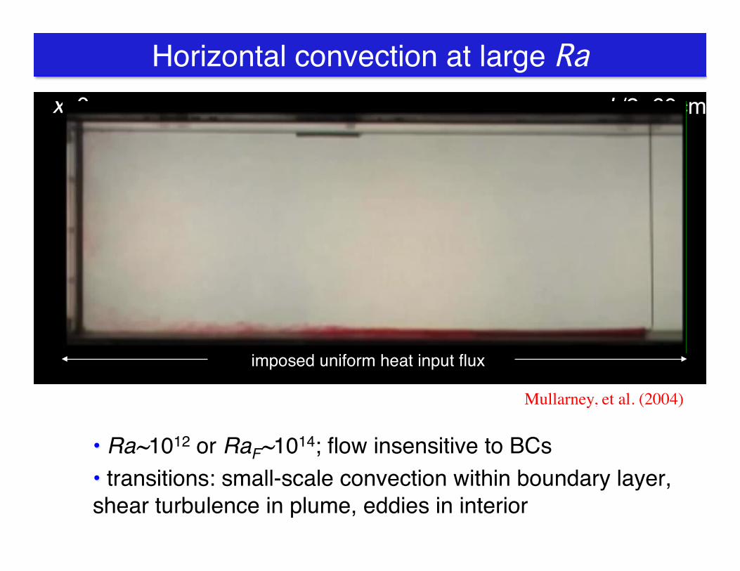
• Ra~1012 or RaF~1014; flow insensitive to BCs!• transitions: small-scale convection within boundary layer, shear turbulence in plume, eddies in interior!
Horizontal convection at large Ra!
Mullarney, et al. (2004)
imposed uniform heat input flux
x=0! L/2=60cm!