The Pennsylvania State University

The Graduate School

OCEAN ECOSYSTEM TRANSFORMATION CAUSED BY RAPID WARMING AND

SEA LEVEL RISE IN THE PLEISTOCENE CARIACO BASIN (MIS 9-7)

A Thesis in

Geosciences

by

Adriana I. Rizzo

Submitted in Partial Fulfillment

of the Requirements for the Degree of

Master of Science

August 2019

ii

The thesis of Adriana I. Rizzo was reviewed and approved* by the following:

Timothy J. Bralower Professor of Geosciences Thesis Co-Advisor

Katherine H. Freeman Evan Pugh University Professor Departments of Geosciences and Chemistry Thesis Co-Advisor

Mark E. Patzkowsky Professor of Geosciences Associate Head for Graduate Programs and Research, Department of

Geosciences

*Signatures are on file in the Graduate School

iii

ABSTRACT

Local phytoplankton community structure has implications for larger ocean ecosystems and the

global carbon cycle. Understanding the response of these ecosystems to warming in the tropics is

important for understanding future global change. We examined changes in phytoplankton

community composition over a full glacial cycle in MIS 9-7 (330-230 kya) in the sediments from

the Cariaco Basin (ODP Site 1002). Phytoplankton communities were reconstructed using both

calcareous nannoplankton assemblages and sterol and alkenone biomarkers. These data were

integrated with alkenone, microfossil, and sterol proxies for temperature and circulation.

Emiliania huxleyi occurred definitively in the Cariaco Basin for the first time between 250 and

240 kya, possibly due to increased connectivity caused by rising sea level. At the same time,

environmental variability increased during a period of rapid warming from 250-240 kyr,

inducing ecological turnover at both species- and larger clade levels. In general, during

interglacials, the basin was more productive and more stratified, suggesting higher nutrient

fluxes from land and greater rainfall associated with a more northerly ITCZ. This suggests that

current warming may cause similar species introductions, productivity changes, and disruptions

to phytoplankton populations.

iv

TABLE OF CONTENTS

LIST OF FIGURES...................................................................................................................... v

LIST OF TABLES........................................................................................................................ vi

ACKNOWLEDGEMENTS.......................................................................................................... vii

Introduction................................................................................................................................... 1

Pleistocene Climate Changes in the Cariaco Basin........................................................... 3

Methods......................................................................................................................................... 7

Taxonomy.......................................................................................................................... 7

Stratigraphy and age model............................................................................................... 8

Organic geochemistry methods......................................................................................... 11

Statistical analyses............................................................................................................ 13

Results........................................................................................................................................... 15

Discussion..................................................................................................................................... 22

Ecological response of taxa to environmental change...................................................... 22

Glacial/Interglacial trends in productivity and nutrient sourcing..................................... 24

Biomarkers and Nannofossils: a new approach for paleoceanographic reconstruction... 27

Sea level change, biogeography, and dispersal of E. huxleyi......................................... 29

Implications for future change.......................................................................................... 31

Conclusions................................................................................................................................... 33

References..................................................................................................................................... 34

Appendix A: Rarefaction analysis of nannofossils ...................................................................... 41

Appendix B: Nannofossil preservation......................................................................................... 44

Appendix C: Multivariate Analysis.............................................................................................. 46

Appendix D: Biomarker data........................................................................................................ 50

Appendix E: Data plotted against depth....................................................................................... 54

v

LIST OF FIGURES

Figure 1: Seasonal changes in the ITCZ position over South America......................................... 4

Figure 2: Map showing location and modern bathymetry of the Cariaco Basin............................ 6

Figure 3: Sedimentation rate and stratigraphy for studied interval of Hole 1002D...................... 10

Figure 4: Climate trends globally and at Site 1002 ...................................................................... 15

Plate 1: SEM micrograph of morphologies that would be identified as E. huxleyi/R. parvula in

the light microscope...................................................................................................................... 16

Figure 5: Relative abundances of calcareous nannofossils........................................................... 17

Figure 6: Rolling variance for major coccolith species, excluding the Emiliania complex......... 19

Figure 7: Percent organic carbon and biomarker Mass Accumulation Rates............................... 21

Figure 8: Schematic showing ecological response of major phytoplankton clades...................... 22

Figure 9: Schematic summarizing interpretation of glacial-interglacial environmental changes. 26

Figure A1: Rarefaction and species accumulation curves for calcareous nannofossils................ 42

Figure A2: Nannofossil rank-abundance curves........................................................................... 43

Figure B1: Coccolith preservation over time................................................................................ 45

Figure C1: NMDS of nannofossil data set, with fitted environmental variables.......................... 47

Figure C2: DCA of nannofossil data set, with fitted environmental variables............................. 48

Figure E1: Relative abundances of calcareous nannofossil and Pielou's evenness metric vs.

depth.............................................................................................................................................. 54

Figure E2: Temperature and biomarker Mass Accumulation Rates plotted against depth........... 55

vi

LIST OF TABLES

Table 1: First differences correlations (ρ) between phytoplankton biomarkers, paleoceanographic

proxies, and nannoplankton relative abundances......................................................................... 20

Table 2: First differences correlations (ρ) between phytoplankton biomarkers........................... 20

Table D1: Concentrations for measured biomarkers.................................................................... 51

Table D2: Parameters used in mass accumulation rate calculations............................................. 52

Table D3: Mass accumulation rates for measured biomarkers..................................................... 53

vii

ACKNOWLEDGEMENTS

I would like to thank my advisors, Kate Freeman and Tim Bralower, for their feedback

and assistance as well as their willingness to support a project slightly out of their usual realm of

research. Thanks as well to Mark Patzkowsky, my third committee member, for his helpful

feedback and for facilitating an excellent environment for scientific conversations with my peers.

This research was supported by several Penn State Geosciences department scholarships:

the Tait Scholarship in Microbial Biogeochemistry, the Shell Research Facilitation Award, and

several Krynine Travel Grants. Thank you to the donors to the department for your generosity.

Additional funding was provided by the National Science Foundation, award # 1416663.

I would also like to thank Yongsong Huang of Brown University for access GC-FID

instruments in his lab, and to Richard Vachula and Xiangming Zhao, also of Brown University,

for assistance running my samples.

Many thanks to the Freeman lab group, particularly Troy Ferland and Allison Karp, for

their thoughtful feedback and assistance with unruly instruments. Thanks also to Sara Lincoln,

Denny Walizer and Margaret Davis for assisting with various instrument and facilities issues.

Finally, thank you to my family and friends for supporting me through this difficult

journey. In particular, thank you Ashwin for your many sacrifices and the support I've had

through my troubles. I couldn't have done it without you.

1

Introduction

Marine phytoplankton ecosystem structures are important components of the Earth

system and are sensitive to climate and ocean circulation. Marine phytoplankton are key

components of the global carbon cycle and the basis for marine food webs. Coastal and

upwelling zones have the highest rates of carbon fixation per square meter (Knauer, 1993). Due

to their productive fisheries and proximity to human settlements, these regions are of particular

importance for human society but also more subject to human influence (Shackeroff et al., 2009).

Three main clades of phytoplankton, dinoflagellates, diatoms, and coccolithophores dominated

these environments throughout the Cenozoic. Each of these groups has distinct preferences for

nutrients and water column stability, an ecological framework referred to as Margalef's Mandala

(Margalef, 1978).

Changes in phytoplankton species distributions and in group rank abundances can affect

the movement of carbon through the ocean and disrupt food webs at higher trophic levels.

Diatoms and coccolithophores enhance carbon flux to the deep sea by ballasting organic matter

with mineral tests (Honjo, 1976), but the rates of this flux are size- and species-dependent (Ziveri

et al. 2007). In particular, coccolithophores are more efficient at ballasting (Thunell et al., 2007)

and provide a significant flux of inorganic carbon to the deep sea via calcification (Ridgewell,

2005). Harmful Algal Blooms (HAB), monospecific assemblages of toxin-producing diatoms

and dinoflagellates, can kill fish and marine mammals, posing economic threats (Hoagland and

Scatasta, 2006) and additional burdens for the conservation of threatened and endangered species

(Fire and Van Dolah, 2012).

Our rapidly warming modern climate is likely to substantially change the geographic

distribution of many phytoplankton, including HAB species (Hallegraeff, 2010; Kordas et al.,

2

2011). However, disentangling the influence of climate and anthropogenic nutrient inputs

presents a challenge. Additionally, it is not clear how coccolithophores, which are mostly

insensitive to temperature (Hagino et al., 2000) and cosmopolitan in their distribution (Okada

and Honjo, 1973), will respond to climate change. In this study, we seek to understand

oceanographic and climate mechanisms driving the distribution of greater phytoplankton groups

and species distribution of coccolithophores during a warming climate.

These predictive challenges can be mitigated by studying the middle Pleistocene record

of climate-ecosystem interaction, which contains all major species of modern coccolithophores.

The glacial cycle from marine isotope stage 9 to stage 7 is of particular interest for biogeographic

studies because it contains the global first occurrence of Emiliania huxleyi (Raffi et al., 2006).

During this time, global temperatures increased by 5°C (Hönisch et al., 2009) and global sea

level rose by 100 m (Dutton et al., 2009; Lea et al., 2002) within 10 kyr. Although the rate of

change is orders of magnitude below the pace of anthropogenic climate change, ecological

changes in high resolution during the relatively swift warming at the onset of the MIS 7

interglacial can provide meaningful context for understanding the future.

The Cariaco Basin, southern Caribbean Sea, has hydrography sensitive to major changes

in climate and ocean circulation. Moreover, high sedimentation rates enable high temporal

resolution sampling on sub-millennial intervals. Geographically, the region experiences a climate

regime that is sensitive to changes in major patterns of ocean and atmospheric circulation. These

changes have been well characterized by previous research on sediments from Ocean Drilling

Program (ODP) Leg 165 at Site 1002, the source of the samples analyzed in this study. We

hypothesize that changes in water column structure and nutrient delivery associated with

3

circulation and sea level changes provided the primary control on phytoplankton ecosystem

structure.

Pleistocene Climate Changes in the Cariaco Basin

The Cariaco Basin is a pull-apart basin located at 10°N on the Caribbean margin of South

America (Figures 1, 2). Today, the Cariaco Basin is noted for its permanent anoxia below 300 m

(Richards and Vaccaro, 1956). During the Northern Hemisphere winter months, when insolation

is at a minimum at 10° north, the Intertropical Convergence Zone (ITCZ) shifts south (Figure

1A), creating strong easterly trade winds that cause advection-driven upwelling on shallow areas

of the Tortuga Bank, the sill on the northern part of the basin (Astor et al., 2003). During the

summer months (Figure 1B), when insolation is at a maximum at 10°N, the ITCZ moves north,

initiating the rainy season nearby in northern South America and weakening the trade winds

(Astor et al., 2003; Muller-Karger et al., 2001). This shuts down upwelling and reduces

thermocline mixing in the basin; increased fresh water inputs cause a transient decrease in

salinity, which is above 36 ppt other times of the year (Astor et al., 2003; Richards and Vaccaro,

1956). Volumetrically, the fresh water flux from small rivers that empty into the Cariaco Basin is

small compared to that of the Orinoco River, which does not directly flow into the basin but is a

major source of terrestrial inputs to the Eastern Caribbean in general (Richards, 1975).

4

Paleoceanographic studies indicate that climate and oceanographic conditions during

previous interglacial periods broadly resembled the present. Multiple proxies indicate anoxia set

in around 14.5 kya in association with increased productivity after the Last Glacial Maximum

(LGM) (Peterson et al., 2000b, 1991; Yarincik et al., 2000a). In contrast, during glacial and

cooler periods, the basin was generally less productive (Herbert and Schuffert, 2000; Peterson et

Figure 1: Seasonal changes in the ITCZ position over South America. The Cariaco Basin is indicated by the blue box. A) ITCZ position in January, when insolation is at a minimum at 10° N. The ITCZ shifts south, creating a pressure difference that causes dry conditions and strong easterly winds over the Cariaco Basin, resulting in upwelling. B) ITCZ position in July, when insolation is at a maximum at 10° N. The zone of low pressure moves towards the Caribbean coast, resulting in high precipitation and runoff and a shutdown of trade winds and upwelling in the Cariaco Basin.

5

al., 2000a, 2000a), even though it also experienced more intense upwelling (González et al.,

2008b; Mertens et al., 2009a, 2009b). This pattern was driven by a combination of lower sea

level and a more southern ITCZ, which strengthened winter upwelling conditions. During the

Younger Dryas, a short period of cooling following the Last Glacial Maximum, the basin was

characterized by both high productivity and enhanced upwelling (Dahl et al., 2004; Herbert and

Schuffert, 2000; Werne et al., 2000), consistent with higher sea level and lower summer

insolation. Reduced rainfall during cold periods decreased forest cover on land (González et al.,

2008a; Hughen et al., 2004; Makou et al., 2007), consistent with a significant shift of the ITCZ to

a more southern location. This southward shift caused decreased rainfall in northernmost South

America and reduced terrestrial runoff to the basin during glacial periods compared to warmer

and wetter interglacials (González et al., 2008a; Haug et al., 2001; Peterson and Haug, 2006).

Cariaco Basin sediments may have also received increased aeolian inputs (Yarincik et al., 2000b)

during warm periods. Thus, terrestrial nutrient sourcing contributed to increased interglacial

productivity.

Sea level varied considerably both globally and in the Cariaco Basin between the MIS 8

glacial period and MIS 9 and 7 interglacials, with implications for the ventilation of the basin.

During the lowest point of the MIS 8 glacial period at 285 kya, sea level dropped up to 100 m

below current levels, before rising to 80 m below modern levels (Grant et al., 2014; Rohling et

al., 2009, 2009), although others estimate the decrease was -60 m (Siddall et al., 2007). During

the MIS 7 interglacial period, sea level rose, reaching 15 m lower than modern by 248 kya

(Dutton et al., 2009). In modern times, the deepest connections across the sill between the

Cariaco Basin and Caribbean Sea are 120 m across the north sill and 146 m on the western edge

6

(Richards and Vaccaro, 1956).

Figure 2: Map showing location of ODP site 1002 and modern bathymetry of the Cariaco Basin, adapted from Peterson et al. (2000b). The modern shoreline is highlighted in red, while a hypothetical MIS 8 maximal lowstand shoreline, assuming -100 m sea levels and modern bathymetry, is shown in blue.

The Cariaco Basin is a pull-apart basin formed through transtension between the El Pilar

and San Sebastian faults, transform faults that run East-West through the basin (Schubert, 1982)

and form part of the boundary between the South American and Caribbean plates. Much of the

subsidence in the Cariaco Basin occurred before early Pliocene, and since then tectonic activity

has shifted towards widening of the eastern lobe of the basin (Escalona et al., 2011). Given this

context, it is unlikely that the sill connections were substantially deeper in the Middle

Pleistocene. Thus it is possible that the Cariaco Basin's only access to the open ocean during

cold glacial periods was through a narrow channel less than 50 m (Figure 2).

This climate dynamic provides several important factors other than temperature that

could have substantially influenced phytoplankton populations. To better understand these

changes and their ecological impact, we coupled high resolution nannofossil assemblage data

7

with biomarker proxies for coccolithophore, diatom, and dinoflagellate productivity and organic

matter sourcing, as well as the alkenone unsaturation index sea surface temperature proxy, UK37'

(Brassell et al., 1986; Prahl and Wakeham, 1987). While other studies have reconstructed

phytoplankton communities in the Cariaco Basin using sterols (Dahl et al., 2004; Werne et al.,

2000) and alkenones (Herbert and Schuffert, 2000), none have examined the MIS 9-7 glacial

cycle. Likewise, Mertens et al. (2009b) presented data on calcareous nannofossil assemblages

but not during the MIS 9-7 glacial cycle. Thus we lack knowledge of phytoplankton during a

key interval for coccolithophore evolution: the global first appearance of Emiliania huxleyi,

previously identified for this site at 248 kya (Peterson et al., 2000b). The combination of

nannofossil and organic geochemical data allows us to assess how sea level, productivity,

temperature, and ecological interactions across both closely and distantly related phytoplankton

fostered range expansion and altered community composition.

Methods

Taxonomy

For nannofossil assemblages, smear slides were counted in cross-polarized light at 1600x

magnification. 300 specimens were counted per slide. This number was selected based on

rarefaction curves (Appendix A) that confirmed that 300 specimens are sufficient to capture the

diversity of the assemblages.

Taxonomy generally follows Okada (2000). Gephyrocapsa was split by size, into small

(2-3 µm), medium (3-5 µm), and large (> 5 µm) categories. We grouped these taxa in

Gephyrocapsa spp. Also following Okada, we separately counted "small placoliths", or

placoliths < 2 µm with thick rims. This category includes small Gephyrocapsa taxa variously

referred to as G. ericsonii (Hagino et al., 2000), G. protohuxleyi (McIntyre, 1970) and G. Minute

8

(Bollmann, 1997) as many specimens had recognizable bridges. This taxonomic grouping is

associated with tropical upwelling zones and has been used as a proxy for paleoproductivity

(Gartner, 1988; Kameo, 2002; Okada, 2000).

Emiliania huxleyi was combined with other, small placoliths (< 2µm) with a thin central

area and lacking a bridge. The miniscule E. huxleyi coccoliths are highly prone to dissolution,

and are difficult to distinguish in the light microscope from species such as Reticulofenestra

parvula. Similar approaches have been taken by other nannofossil workers (Cabarcos et al.,

2014; Rogalla and Andruleit, 2005). Additionally, recent phylogenetic work suggesting

extensive hybridization between Emiliania, R. parvula, and Gephyrocapsa (Bendif et al., 2016,

2015) casts further doubt on the evolutionary significance of dividing species within the

Noelaerhabdaceae. However, we continued to separate Emiliania and Gephyrocapsa due to their

distinct ecologies and biogeography in the modern ocean (Okada and Honjo, 1973).

Helicosphaera, Pontosphaera, and Syracosphaera were identified at the genus level only.

Other species counted were Florisphaera profunda, Rhabdosphaera claviger, Calcidiscus

leptoporus, Umbilicosphaera hulburtiana, and Reticulofenestra sp. >3 µm.

Stratigraphy and age model

Five holes (A-E) were drilled at Site 1002, which is located on the central saddle of the

basin (Figure 2), where seismic stratigraphy suggests continuous, flat deposition free from

slumping (Sigurdsson et al., 1997). Each hole was cored to 180 m, equivalent to 600 kyr, which

demonstrates an average sedimentation rate of 35 cm/kyr. The section consists of a single grey-

brown silty clay unit, which was divided into six subunits on the basis of microfossils. All of our

samples come from subunit E, a thick and homogenous greenish gray to dark greenish gray

9

nannofossil silty clay, with the exception of the lowermost 0.5 m, which come from subunit F, a

dark olive green nannofossil silty clay with diatoms. The carbonate content in the studied

interval averaged 27.8%.

10

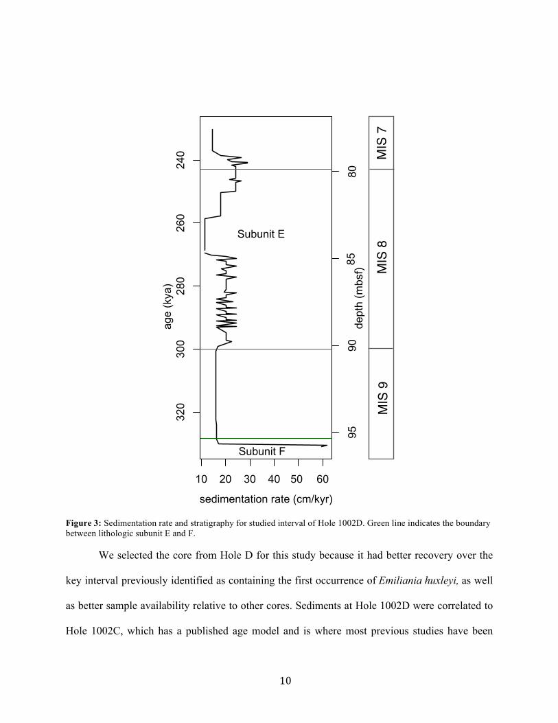
We selected the core from Hole D for this study because it had better recovery over the

key interval previously identified as containing the first occurrence of Emiliania huxleyi, as well

as better sample availability relative to other cores. Sediments at Hole 1002D were correlated to

Hole 1002C, which has a published age model and is where most previous studies have been

10 20 30 40 50 60

320

300

280

260

240

sedimentation rate (cm/kyr)

age

(kya

)

9590

8085

Subunit E

Subunit F

dept

h (m

bsf)

MIS

9M

IS 8

MIS

7

Figure 3: Sedimentation rate and stratigraphy for studied interval of Hole 1002D. Green line indicates the boundary between lithologic subunit E and F.

11

conducted, using high-resolution magnetic susceptibility data (Sigurdsson et al., 1997). The

Hole 1002C age model (Peterson et al., 2000c) was based on oxygen isotopes of the planktonic

foraminifera Globigerinoides ruber and the SPECMAP time scale (Imbrie et al., 1984). The age

model had an average resolution of 7 kyr over the interval of this study, so dates were linearly

interpolated. Cores were correlated using the R package Astrochron (Meyers, 2014). The average

sedimentation rate in the dataset was 19.0 cm/kyr, with a minimum of 11.5 cm/kyr and a

maximum of 61.9 cm/kyr (Figure 3).

Organic Geochemistry Methods

Extraction methods for biomarkers generally follow the Bligh-Dyer method modified by

Wakeham and Pease (2004). Approximately 5 g of powdered, dry sediment were sonically

extracted three times in a 3:1 by volume azeotrope of dichloromethane and methanol. The total

lipid extract (TLE) was concentrated under N2 to near-dryness. One third of this lipid extract was

archived, and the remainder was saponified for two hours using 0.5 N potassium hydroxide in a

3:1 azeotrope of methanol to water. This mixture was then diluted to half its original

concentration with 5% NaCl, then extracted three times with hexane to produce the neutral

fraction. The pH of the aqueous phase was adjusted with hydrochloric acid to less than two, and

extracted three times with hexane to produce the acid fraction, which was archived without

analysis.

For sterol analysis, aliquots of the saponified neutral fraction were derivitized with

bistrimethylsilyltrifluoroacetamide (BSTFA) and pyridine for 60 minutes at 60° C to stabilize

sterols and alcohols. Androstane was added as internal standard to a concentration of 10 ng/µL.

The derivitized neutral fractions were analyzed on an HP 5973 mass spectrometer coupled to an

12

Agilent 6890 series gas chromatograph. Samples were injected with a splitless injection onto a

30 m, 0.25 mm diameter DB-XLB column with a 0.25 µm film thickness (Agilent), with an

initial oven temperature of 90°C followed by a ramp of 8°/minute to temperature of 300°,

followed by a ramp of 1°/minute to a final temperature of 320°. Sterols were identified by

retention time and mass spectra comparison to a standard mix consisting of cholesterol (Baker),

13% brassicasterol, 26% campesterol, 7% stigmasterol, 53% β-sitosterol (Indofine). Dinosterol

was identified by comparison to previously published retention order and spectra (Volkman et

al., 1990).

Alkenones were quantified on an Agilent 6890N gas chromatograph with Flame

Ionization Detection using splitless injection on a 60 m by 0.25 mm by 0.25 µm RTX-200 ms

column (Restek) at Brown University, with an initial oven temperature of 50°C held for 2 min,

followed by a 20°C/min ramp to 255° and then a ramp of 3°C /min to 320°C, held for 25 min, as

per Zheng et al. (2017).

Biomarker concentrations were calculated based on the ratio of peak areas to the internal

standard, androstane. Concentrations were converted to Mass Accumulation Rates (MARs) by

multiplying biomarker concentrations in nanograms per gram sediment times linear

sedimentation rates (cm/year; calculated for hole D based on the age model and correlation with

Hole 1002C) and bulk density (g/cm3) measured by the original ODP sampling party (Sigurdsson

et al., 1997).

Sea surface temperatures were estimated using the UK'37 alkenone unsaturation index

(Prahl and Wakeham, 1987):

UK'37 = C37:2/(C37:2+C37:3) (1)

13

Sea Surface Temperatures were calculated based on the calibration for Gephyrocapsa oceanica

(Volkman et al., 1995) because this species is numerically more abundant throughout the section

and in modern tropical environments than Emiliania (Okada and Honjo, 1973). The calibration

equation is as follows:

SST (°C) = (Uk’37 +0.520) × 20.41 (2)

These values were compared to mean daily insolation on February 15 at 10° N and

obliquity, which were calculated with the solution of Laskar et al. (2004) using the software

program Acycle (Li et al., 2019), as well as globally averaged trends in temperature and ice

volume via the LR04 benthic oxygen isotope stack (Lisiecki and Raymo, 2005).

Organic carbon, organic nitrogen, and carbonate contents were not measured in this

study. Instead, we employed previously measured values from Hole C (Haug et al., 1998). These

measurements were at a slightly higher resolution than our biomarker data set (average

resolution 2.1 vs. 4.6 kyr) and each point in our data was compared to the closest point in time.

Statistical Analyses

Statistical analyses, which included calculations of correlation and moving window

variance, were performed in R. All correlation coefficients given are Spearman's ρ, and all

correlations or regressions were performed on the first differences of the data to avoid spurious

relationships caused by temporal autocorrelation. Rolling variance was performed using the

package roll.

Pielou's evenness metric, J, which is defined as follows, was also calculated.

J = H/ln 𝑆 (3)

H is the Shannon Diversity Index, defined as

14

H = - 𝑝! ln𝑝!!!!! (4)

where pi is the proportional abundance of the ith species. S is the total number of species in the

assemblage. J ranges from 0 to 1, with higher values indicating a more even assemblage.

15

Results

Sea surface temperatures estimated from alkenones for Site 1002 followed global

temperature trends (Figure 4); the gradual cooling trend from MIS 9 into MIS 8 was interrupted

by transient warming around 280 kya. After a temperature minimum of 21.4° C at 260 kya, sea

surface temperatures increased rapidly to a maximum of 27.7° at 242 kya. These trends slightly

lead but generally follow the LR04 stack, which represents globally averaged deep sea

temperature and ice volume. Trends in SST generally followed winter (February 15) insolation,

370 400

320

300

280

260

240

insolation (W/m2

)

ag

e (

kya

)

��

��

��

����

��

��

���

��

��

��

��

�����

�����

��

���������

���

��

�����

�����

��

���

��

�����

����

���

��

��

��

��

��

���

������

�

4.6 4.0 3.4

δ18O, ‰

�

��

��

�

�

�

�

�

�

�

�

�

�

��

�

�

�

�

�

22 24 26

SST (°C)

MIS

8M

IS 7

MIS

9

Figure 4: Climate trends globally and at Site 1002. Left: mean insolation on February 15 at 10°N. Center: LR04 global benthic oxygen isotope stack (Lisiecki and Raymo, 2005). Right: Sea surface temperatures at Site 1002 based on the UK'

37 alkenone unsaturation index. Marine Isotope Stage (MIS) chronology is indicated on the right.

16

which makes sense as winter insolation determines the strength of the southern ITCZ and the

strength of upwelling in the Cariaco Basin.

Plate 1: SEM micrographs of morphologies that would be identified as E. huxleyi/R. parvula in the light microscope. A-C from 241.0 kya, proximal view; A and B show Emiliania huxleyi sensu stricto features, notably a perforated, "hammerhead" distal shield. A-C are almost identical in proximal view. D-F from 250.9 kya; the thick inner cycle of D coupled with thin rim would closely resemble Emiliania huxleyi sensu stricto in the light microscope. G-I from 300.7 kya, showing morphology typical of R. parvula.

SEM imaging (Plate 1) revealed that many specimens that resembled Emiliania huxleyi in

the light microscope were likely in actuality Reticulofenestra parvula, a closely related species.

Henceforth, we refer to these two species together as the Emiliania complex. Preservation was

17

adequate but not perfect throughout this section (Appendix 2), and if dissolution removed the

fragile distal shield of E. huxleyi, it would leave only the thicker inner rim and the specimen

woul resemble R. parvula (Plate 1H), as the proximal shields of the two are virtually identical

(Plate 1B, C). The only unambiguous specimens of E. huxleyi were observed at 241.0 kya.

Nevertheless, there is a substantial increase in the relative abundance of the Emiliania complex

(Figure 5), which suggests a shift in ecology in the group.

Figure 5: Relative abundances of calcareous nannofossil and Pielou's evenness metric

Nannofossil abundances broadly follow ocean temperatures. While the 280 kya warming

was not accompanied by change in nannofossil assemblage data, the warming at 260 kya

correlated with pronounced upheaval in the abundance of all major nannofossils (Figure 5).

��

�

��

�� ����� ��� ���� �� � ����

����� �� � �� ����� ���������

��������������������� �����������������

�

�

����

���

�

�

�

�

�

�

�

���

0 40 80

age

(kya

)

��

�

��

�� �� �� ���� � ������ �� ��

� ���� �� � ��� �� � ����� �� � ���� ��� ������ ��� ����������� �

����� �� �

�� �

��

�

��

��

���

�

�

�

�

�

�

�

� ��

0 40 80

���

���

������� � ��� � �� �� ��� �� ��� ��� �������� � �

������������������������� ������ ��

������� �

���

��

�

��� �

���

�

�

�

�

�

�

�

���

0 40 80

��

�

��

�� � ����� ���� �� � ��� �� ��� � � �� ��� ��� ��� ��

� �� ����� �� ��������� � �� �� �� ��� ����

��

� � �� �����

��

�

����

�� �

�

�

�

�

�

�

�

�� �

0 40 80

���

��

������������������������ ����������������������� �������������������������

�������

�����

�

����

���

�

�

�

�

�

�

�

���

0 40 80

��

�

��

�� ��� ��� �� �� �� �� ���� �

�� � �� �� ����� ��� ����� ������� � ���� ���� ��� � �� ������ ��

������ ��

���

��

�

��� �

���

�

�

�

�

�

�

�

�� �

0.0 Pielou's evenness (J)relative abundance, %

MIS 8

MIS 7

MIS 9

Emiliania complex small placoliths F. profunda

Gephyrocapsa spp. other

320

300

280

260

240

1.0

18

Notably at this time, the Emiliania complex, a minor component of the assemblage for most of

the studied interval, increased in abundance to 30%. The abundances of other major components

of the assemblage, the small placoliths, Florisphaera, and Gephyrocapsa, fluctuated

significantly. As seen in Figure 6, temporal variability in nannofossil abundances increased

during this interval.

19

Mass Accumulation Rates of all major biomarker classes increased during warm periods

but individual compound groups followed the trend of SST and global δ18O values to different

degrees (Figure 7). Brassicasterol and brassicastanol, two structurally similar biomarkers for

diatoms were highly correlated (ρ = 0.834) with each other and the pair are hereby referred to as

diatom sterols. This compound group had the strongest relationship with temperature. Dinosterol,

by far the most abundant of any biomarker here, weakly correlated with temperature and other

Figure 6: Rolling variance for major coccolith species, excluding the Emiliania complex, which sharply increases following the temperature minimum at 260 kya. Calculated with a rolling window with a constant n=7. Since temporal resolution decreases with age in this data set, the amount of time averaged decreases up section.

0.00 0.02 0.04 0.06 0.08

320

300

280

260

240

age

(kya

)

small placoliths

F. profunda Gephyrocapsa spp. other

MIS 7

MIS 8

MIS 9

20

biomarkers. Similarly, the combined abundances of C37:2 and C37:3 alkenones (hereafter referred

to as ΣC37) weakly correlated with alkenone temperature estimates. Additionally, dinosterol

strongly correlated with the relative abundance of F. profunda. None of the biomarkers

correlated well with other nannofossil taxa, % total organic carbon (TOC), or each other (Table

2).

Table 1: First differences correlations (ρ) between phytoplankton biomarkers, paleoceanographic proxies, and nannoplankton relative abundances.

SST (°C)

β-sitosterol MAR

% TOC Emiliania complex relative abundance

small placoliths relative abundance

F. profunda relative abundance

Gephyro-capsa spp. relative abundance

dinosterol MAR

0.160 0.276 0.126 -0.211 -0.205 0.537 -0.375 ΣC37

MAR 0.199 0.201 -0.117 0.103 0.291 -0.007 0.216

Brassica-stanol + stenol MAR

0.564 0.912 0.122 0.103 0.456 -0.015 -0.401

Table2:First differences correlations (ρ) between phytoplankton biomarkers.

dinosterol MAR ΣC37 MAR Brassicastanol + stenol MAR

dinosterol MAR 1 -- -- ΣC37 MAR 0.170 1 -- Brassicastanol + stenol MAR

0.375 0.062 1

21

Figure 7: Percent organic carbon and biomarker Mass Accumulation Rates. Left: Alkenone unsaturation index (UK

37') estimates of Sea Surface Temperature (SST). Second Left: Percent Total Organic Carbon (Haug et al., 1998). All others are Mass Accumulation Rates (MAR) of different biomarker classes: Dinosterol is a C30 sterol produced by dinoflagellates. Total C37 alkenones (the sum of the C37:3 and C37:2 alkenones) are produced by Noelaerhabdacean haptophytes, likely Gephyrocapsa. Brassicasterol and brassicastanol, a diagenetic product of the former, are both C28 stenols associated with diatoms, particularly Thalassiosira. β-sitosterol is a C29 sterol produced predominantly by plants and interpreted as a marker for terrestrially-sourced organic matter.

�

�

�

�

�

�

�

�

�

�

���

���

����

�

�

�

�

�

��

�

�

�

�

�

�

��

��

�

�

�

�

�

�

��

�

�

�

0 1 2 3

32

03

00

28

02

60

%TOC

age (

kya)

�

��

��

�

�

�

�

�

�

�

�

�

�

��

�

�

�

�

�

0 500 1500

dinosterol

MAR (ug/cm/kyr)

�

��

��

�

�

�

�

�

�

�

�

�

�

��

�

�

�

�

�

0 200 400

ΣC37

alkenones

�

��

��

�

�

�

�

�

�

�

�

�

�

��

�

�

�

�

�

brassicastanol

+stenol

�

��

��

�

�

�

�

�

�

�

�

�

�

��

�

�

�

�

�

0 5 10 20

β sitosterol

0 20 40

MIS

8M

IS 7

MIS

9

�

��

��

�

�

�

�

�

�

�

�

�

�

��

�

�

�

�

�

22 24 26

24

0

SST (°C)

22

Discussion

This data set shows evidence for profound changes in ecology and climate between cool

and warm periods in the Cariaco Basin.

Ecological Response of taxa to environmental change

Figure 8: Schematic showing ecological response of major phytoplankton clades in accordance with Margalef's Mandala. Top right shows a rendering of Margalef's Mandala (Margalef 1978) with proxies used in this study superimposed on the plot. F. profunda relative abundance is a proxy for turbulence and β-sitosterol mass accumulation rate as a proxy for nutrient inputs. Smaller plots cross plot the first differences of proxies for phytoplankton clades against these proxies: A) diatoms (brasssicastanol+stenol) vs. nutrient input (β sitosterol); coccolithophores (C37 alkenones) vs nutrient input (B); and coccolithophores (C37 alkenones) vs stratification (% F. profunda (C); and D) dinoflagellates (dinosterol) vs. stratification (% F. profunda).

23

While all indicators for phytoplankton groups responded to ocean warming, each major

plankton group responded differently and in accord with existing models of their ecology (Figure

8). Margalef's Mandala (Margalef, 1978) delineates a classic view of the ecological preferences

of the three main plankton groups: dinoflagellates occupy a low turbulence, low nutrient zone,

diatoms a high turbulence, high nutrient zone, and coccolithophores an intermediate zone for

both properties. Taking plant-derived β-sitosterol MAR as a proxy for terrestrial-sourced nutrient

inputs, and the relative abundance of F. profunda as a proxy for stratification, our data support

the Margalef model of ecological response as a key driver of changes in abundance of the three

types of phytoplankton over time. Diatom sterol and β-sitosterol MARs were highly correlated

while dinosterol (Table 1), suggesting that diatom production of organic matter was strongly

driven by surface nutrient inputs. Total C37 alkenone abundances were uncorrelated with β-

sitosterol, consistent with an intermediate or generalist affinity to nutrient inputs. In contrast,

dinosterol MARs were highly correlated with F. profunda relative abundance, suggesting that

dinoflagellate production was enhanced during warm periods characterized by stratified

conditions. F. profunda is a deep thermocline dweller that has been used as a proxy for

stratification and a deep nutricline (McIntyre and Molfino, 1996; Molfino and McIntyre, 1990)

or turbidity (Ahagon et al., 1993). In contrast, diatom and coccolithophore biomarker MARs

showed little relationship with F. profunda abundance, suggesting insensitivity to stratification.

Biomarker mass accumulation rates suggest that dinoflagellates were the principle

primary producers throughout MIS 9-7 and especially during interglacials. These findings are

consistent with the results of González et al. (2008b), who observed an increase in autotrophic

dinocysts during interglacials in MIS 3-4 and interpreted this as a signal of stratification. We

caution that β-sitosterol can be produced by certain diatoms (Volkman, 1986), complicating this

24

interpretation. Further work should incorporate additional proxies for plant organic matter such

as n-alkanoic acids in order to verify the relationship between diatoms and terrestrial inputs.

In contrast to other nannofossil taxa, the Emiliania complex shows a monotonic increase

with little short-term variation despite dramatic environmental changes in the 250-240 kya

warming period. This supports an interpretation of Emiliania as a generalist (as opposed to an

obligate eutrophic taxon)-- the exact ecology one would expect this variable environment to

select for. This is consistent with a range of modern studies (Andruleit and Rogalla, 2002; Balch,

2004; Ziveri and Thunell, 2000) that have shown insensitivity or contrary response to upwelling.

As Emiliania does not have a consistent relationship with upwelling, we recommend against its

use as a proxy for upwelling (e.g. Mertens et al., 2009b; Stoll et al., 2007).

Glacial/Interglacial trends in productivity and nutrient sourcing

The large increase in biomarker mass accumulation rates starting around 250 kya

suggests an increase in productivity and nutrient delivery to the Cariaco Basin, but what was the

mechanism for this? While biomarker compound mass accumulation rates generally increased

with warmer temperatures, only diatom sterols have a meaningful correlation with temperature,

suggesting other oceanographic factors may also be significant. Anomalously low SSTs at 260

kya coupled with very low relative abundances of F. profunda suggest upwelling was enhanced

in the basin during this cold period. This is consistent with previous models (González et al.,

2008b; Mertens et al., 2009a, 2009b) and suggests a stronger southern winter ITCZ during

glacial periods. This is supported by modern climatology: southern displacement of the ITCZ

position during winter months fosters upwelling conditions in the Cariaco. The paradox that

more intense upwelling was coupled with indicators of low productivity such as lower biomarker

25

accumulation rates during glacial periods can be resolved by isolation of the Cariaco Basin from

Caribbean waters. During the glacial low stand, the shallow sill (Tortuga Bank) was more

exposed such that only a shallow conduit connected the basin to the open ocean. With depths

less than 70 m, only nutrient-depleted surface waters could be delivered to the basin across the

shallow connection to the open ocean (Haug et al., 1998; Peterson et al., 1991). The lack of

connectivity restricted marine nutrient delivery during cool periods and resulted in lowered net

production. As the sill prevents lateral advection of deep marine waters both today and in the

past, any water upwelled in the Cariaco Basin during glacial periods would have been recycled

from nutrient-depleted water sourced from the basin itself.

During warm periods, increased terrestrial inputs suggest a mechanism for increased

productivity. The concentration of β-sitosterol, a compound produced by higher plants (Meyers,

1997) increased during interglacials and the transient 280 kya warming period. This suggests

increased terrestrial runoff carried more organic matter and nutrients into the basin during

warmer times. This scenario is consistent with evidence from pollen and n-alkanes for increased

forest cover (González et al., 2008a; Hughen et al., 2004), and evidence from sedimentology

(Peterson and Haug, 2006) for increased riverine fluxes, that together reinforce that interglacials

the northern reaches of South America were wetter, likely due to a more northern ITCZ

enhancing the summer climate regime.

During the warming period from 250-240 kya, the basin was more stratified than it was

during glacial maximum, as evidenced by increased abundances of F. profunda, a proxy for

stratification, and stronger terrestrial signals. However, nannofossil abundances during the 250-

240 kya interval were highly variable, including the small placolith group. This taxa has been

considered an upwelling or eutrophication indicator (Gartner, 1988; Kameo, 2002; Okada, 2000).

26

In our data, they had a strong anti-correlation (ρ = -0.606) with Florisphaera. This anti-

correlation suggests alternating periods of stratification and upwelling fueled variability in

productivity.

This inferred alternation between stratification and mixing induced high turnover in the

entire nannofossil assemblage, creating a rapid succession of taxa during the 250-230 kya

interval. The same ecological variability and intense stratification was not observed during the

InterglacialGlacial

Inte

rpreta

tion

Evid

ence

sill sill

Lower β sitosterol MAR

Lower sedimentation rate

Lower biomarker accumula-tion rates

Lower F. profunda abun-dance

Anomalously low SSTs

Higher β sitosterol MAR (pollen & plant waxes from other interglacials)

Higher sedimentation rate

Lower biomarker accumula-tion rates

Higher F. profunda abun-dance

Increased connectivityHigher freshwater inputs

More nutrient inputsStratifiedMore intense July ITCZ

RestrictedHigher salinityNutrient StarvedUpwelling Enhanced

More intense Feb. ITCZ

Figure 9: Schematic summarizing interpretation of glacial-interglacial environmental changes.

27

earlier (280 kya) warm period, although this may be a product of lower temporal resolution in

the nannofossil data set over this interval. This suggests that in this climate regime, rapid

warming increases variability and causes a shift between stratified and mixed oceanographic

modes, destabilizing the entire phytoplankton ecosystem.

Biomarkers and Nannofossils: a new approach for paleoceanographic reconstruction

Integrating biomarker and nannofossil proxies presents a promising approach for

paleoceanographic reconstruction. However, a comparison between two different methods of

reconstruction underscores the limitations that come from differences in the nature of the

proxies. Coccolithophore ecology was evaluated using two different methods: total C37

alkenones, which in marine environments are produced by coccolithophores in the family

Noelrhabdaceae, principally G. oceanica and E. huxleyi, and calcareous nannofossil relative

abundances. The ΣC37 alkenone accumulation rate had no correlation with either G. oceanica or

the E. huxleyi complex, emphasizing that production or preservation biases influence organic and

inorganic forms differently. Of all nannoplankton species, alkenones had the strongest

correlation with Calcidiscus leptoporus (ρ = 0.443), an unrelated species that is not known to

produce alkenones today. This points to the complications of comparing these disparate metrics

of similar phenomena; relative abundance versus mass accumulation rates. Additionally, not all

genotypes of alkenones-producers create coccoliths (Rokitta et al., 2011), so coccolith counts

may not accurately estimate alkenone production. This is consistent with previous studies that

have shown that the UK'37 alkenone proxy is not sensitive to nannofossil assemblage changes

(Jordan et al., 1996; McClymont et al., 2005).

28

Due to production and dissolution biases, nannofossil assemblages may not be

representative of total production, but they still provide a wealth of information about relative

changes in oceanography that biomarkers cannot. Biomarker proxies for temperature and organic

matter sourcing are well developed, but are seasonally and spatially averaged in marine settings.

Nannofossil proxies can provide additional valuable information about water column structure.

Combining both provides a more complete, three-dimensional reconstruction of

paleoceanographic variables than either alone.

The sterol biomarker approach to community reconstruction, while coarse, allows for

comparison across disparate clades, moving us closer to an accounting of the ecology of the

entire phytoplankton community. Diatom, dinoflagellate, and coccolithophore microfossils all

have different production and preservation conditions, making quantitative comparisons difficult,

and these conditions vary considerably even within coccolithophores (Young et al., 2005). Our

combined biomarker-nannofossil approach shows promise in elucidating the ecologies of extinct

species of calcareous nannofossils, particularly if combined with multivariate methods. Placing

extinct species in a turbidity- surface productivity space, as we have done here, could help test

hypotheses about important problems such as mechanisms for floral change during other periods

global change (i.e. Eocene hyperthermals) or long term trends in diversity among other algal

clades. These methods should be applicable throughout the Cenozoic, as the long-ranging

Cenozoic genus Discoaster was replaced by F. profunda and is thought to share a similar

ecology (Schueth and Bralower, 2015).

29

Sea level change, biogeography, and dispersal of E. huxleyi

Due to taxonomic uncertainty, we cannot definitively identify the first occurrence of

Emiliania huxleyi sensu stricto, but the sudden increase in abundance at 250 kya is highly

suggestive of dramatic ecological or evolutionary changes. This increase should not be confused

with the Emiliania huxleyi acme, which occurred diachronously at 60-80 kya (Raffi et al., 2006;

Thierstein et al., 1977), above the interval of this study. Globally, E. huxleyi first occurred at

open ocean sites at 291 kya (Raffi et al., 2006), later than our first observations of the Emiliania

complex (at 330.1 kya) but earlier than this increase in abundance. Our SEM images provided no

evidence for Emiliania huxleyi, sensu stricto, from 250.9 kyr or before (Plate 1). Previous work

at Site 1002 (Peterson et al., 2000b) also reported the first occurrence of Emiliania huxleyi at 248

kya. Two explanations are compatible with the later appearance: either environmental instability

associated with warming at 250 kya allowed Emiliania huxleyi, sensu stricto, a previously rare

species, to become more abundant, or sea level rise at 250 kya introduced E. huxleyi s.s. into the

Cariaco Basin for the first time.

The first, ecological hypothesis posits that Emiliania huxleyi, sensu stricto was

cryptically introduced somewhere near the global datum, but only became ecologically important

once climate warmed and disrupted the coccolithophore ecosystem around 250 kya. The increase

in abundance of the Emiliania complex at 250 kyr coincides with dramatic changes in circulation

and nutrient supply that led to high variability in the abundance of other nannofossil taxa.

Emiliania is a generalist (Andruleit and Rogalla, 2002; Balch, 2004; Ziveri and Thunell, 2000;

this study), an ecology that would have succeeded in this highly variable, unstable environment.

Alternately, E. huxleyi s.s. may have been introduced late, around 250 kya, due to

biogeographic barriers. Studies of Emiliania huxleyi first occurrences elsewhere (Rio et al.,

30

1990; Sato et al., 1991; Thierstein et al., 1977) generally observed a sudden first appearance, as

opposed to the long period of rarity before a sudden increase we see in the Emiliania complex. If

E. huxleyi s.s. followed this a similar in the Cariaco Basin, the long period of rarity may have

consisted solely of R. parvula or similar forms, while the sudden increase corresponded to the

first occurrence of E. huxleyi s.s.

Specifically, reduced connectivity with the open ocean due to lower sea level delayed the

dispersal of Emiliania huxleyi sensu stricto into the basin. During the MIS 8 glacial period, sea

levels likely ranged between -80 m and -100 m below modern (Grant et al., 2014), and the

Cariaco Basin is separated from the Caribbean Sea by a 100 m deep sill, which would have

restricted marine inflow to two narrow channels <50 m deep, with some very shallow flow over

the sill depending on the magnitude. During glacial periods, the smaller volume of ocean water

reaching the Cariaco Basin due to low sea levels would have statistically reduced the likelihood

that new coccolithophore populations would reach the basin in sufficient abundance to compete

with established populations. As sea level rose, the volume of exchange with the open ocean

increased concurrently with other changes in the oceanographic regime.

Under 80-100 m sea level changes, the Cariaco Basin would not have been fully isolated

but would have experienced reduced marine influence, decreasing the likelihood of introducing

new populations and altering oceanographic conditions (discussed in the the previous section).

Reduced connectivity to the Caribbean Sea would have reduced nutrient inputs and increased

salinity (Peterson et al., 1991), due to decreased marine and freshwater input in a tropical

environment with high evaporation. Nannofossil relative abundances (Figure 5,6) were not

sensitive to the onset of lower sea level but changed dramatically when the climate warmed and

sea level rose. Sea level fell much more gradually than it rose (e.g., Grant et al., 2014), so the

31

lack of response to slow cooling suggests that coccolithophores are able to adapt to a range of

conditions if the pace of change is slow, but not to swifter changes. Modern coccolithophore

community composition in the Arabian Sea, which has variable upwelling and salinity ranges

similar to the Cariaco Basin, is controlled more by productivity than by salinity (Andruleit and

Rogalla, 2002), so we suggest that the changes in community composition at 250 kyr in the

Cariaco Basin were similarly driven by rapid changes in the volume and spatial distribution in

nutrient inputs rather than lowered salinity. While cell abundance in modern E. huxleyi is not

sensitive to salinity, coccolith number and shape is (Bollmann and Herrle, 2007; Fielding et al.,

2009). However, while E. huxleyi produces larger and more abundant coccoliths under higher

salinity conditions, compelling evidence for E. huxleyi s.s. appears in the Cariaco Basin

concurrently with interpreted decreases in salinity, suggesting that the trend is not caused by

salinity-driven preservational differences.

Disentangling the influence of sea level and climate changes associated with sea level

remains a challenge in paleoceanography, as does disentangling ecological and environment in

paleobiology. Despite these limitations, the hypothesis that E. huxleyi s.s. emerged later in the

Cariaco Basin than in the open ocean due to the basin's relative isolation during glacial periods is

consistent with all available evidence.

Implications for future change

In this study, we found that warming in the Cariaco Basin was associated with increased

productivity and nutrient loading, and ecological variability in phytoplankton. While some of

these changes were enhanced by insolation and may not directly apply to anthropogenic climate

change, others may be of use for policymakers and forecasters of the future. In particular,

32

stratification and nutrient delivery in tropical coasts like the Cariaco Basin may be enhanced by

future warming due to higher sea surface temperatures and increased precipitation (Hallegraeff,

2010; Wells and Karlson, 2018). These temperature-triggered stressors may be further enhanced

by anthropogenic nutrient loading and land use changes that increase erosion (Glibert et al.,

2018). An important takeaway from this study is that intervals of rapid warming coincide with

highly variable environments which lead to ecological variability in phytoplankon. Together with

the enhanced prospects for introduction of new populations due to sea level rise, this heightened

variability and nutrient loading may increase the frequency of harmful algae blooms in

environments like the Cariaco Basin.

33

Conclusions

Both calcareous nannofossil and organic geochemical reconstructions of plankton

ecosystems in the Cariaco Basin showed pronounced ecological disruption following the

initiation of rapid warming at 250 kya, but were fairly insensitive to gradual cooling or lower-

amplitude warming earlier in MIS 8. This coincided with the introduction of Emiliania to the

Cariaco Basin, which was enabled by rising sea level and increased connection to the open

ocean. Sea level rise and increasing terrestrial runoff increased both productivity and

stratification, consistent with a more intense northern ITCZ during interglacial periods. Overall,

the period of warming at the end of MIS 8 was characterized by increased environmental

variability. The entire interval was dominated by dinoflagellate productivity.

34

References Ahagon, N., Tanaka, Y., Ujiie´, H., 1993. Florisphaera profunda, a possible nannoplankton

indicator of late Quaternary changes in sea-water turbidity at the northwestern margin of the Pacific. Mar. Micropaleontol. 22, 255–273. https://doi.org/10.1016/0377-8398(93)90047-2

Andruleit, H., Rogalla, U., 2002. Coccolithophores in surface sediments of the Arabian Sea in relation to environmental gradients in surface waters. Mar. Geol. 186, 505–526. https://doi.org/10.1016/S0025-3227(02)00312-2

Astor, Y., Muller-Karger, F., Scranton, M.I., 2003. Seasonal and interannual variation in the hydrography of the Cariaco Basin: implications for basin ventilation. Cont. Shelf Res. 23, 125–144. https://doi.org/10.1016/S0278-4343(02)00130-9

Balch, W.M., 2004. Re-evaluation of the physiological ecology of coccolithophores, in: Coccolithophores: From Molecular Processes to Global Impact. Springer-Verlag, Berlin, Heidelberg, pp. 165–190.

Bendif, E.M., Probert, I., Díaz-Rosas, F., Thomas, D., van den Engh, G., Young, J.R., von Dassow, P., 2016. Recent Reticulate Evolution in the Ecologically Dominant Lineage of Coccolithophores. Front. Microbiol. 7. https://doi.org/10.3389/fmicb.2016.00784

Bendif, E.M., Probert, I., Young, J.R., von Dassow, P., 2015. Morphological and Phylogenetic Characterization of New Gephyrocapsa Isolates Suggests Introgressive Hybridization in the Emiliania/Gephyrocapsa Complex (Haptophyta). Protist 166, 323–336. https://doi.org/10.1016/j.protis.2015.05.003

Bollmann, J., 1997. Morphology and biogeography of Gephyrocapsa coccoliths in Holocene sediments. Mar. Micropaleontol. 29, 319–350. https://doi.org/10.1016/S0377-8398(96)00028-X

Bollmann, J., Herrle, J.O., 2007. Morphological variation of Emiliania huxleyi and sea surface salinity. Earth Planet. Sci. Lett. 255, 273–288. https://doi.org/10.1016/j.epsl.2006.12.029

Brassell, S.C., Eglinton, G., Marlowe, I.T., Pflaumann, U., Sarnthein, M., 1986. Molecular stratigraphy: a new tool for climatic assessment. Nature 320, 129–133. https://doi.org/10.1038/320129a0

Cabarcos, E., Flores, J.A., Singh, A.D., Sierro, F.J., 2014. Monsoonal dynamics and evolution of the primary productivity in the eastern Arabian Sea over the past 30ka. Palaeogeogr. Palaeoclimatol. Palaeoecol. 411, 249–256. https://doi.org/10.1016/j.palaeo.2014.07.006

Chao, A., Gotelli, N.J., Hsieh, T.C., Sander, E.L., Ma, K.H., Colwell, R.K., Ellison, A.M., 2014. Rarefaction and extrapolation with Hill numbers: a framework for sampling and estimation in species diversity studies. Ecol. Monogr. 84, 45–67. https://doi.org/10.1890/13-0133.1

Dahl, K.A., Repeta, D.J., Goericke, R., 2004. Reconstructing the phytoplankton community of the Cariaco Basin during the Younger Dryas cold event using chlorin steryl esters. Paleoceanography 19, PA1006. https://doi.org/10.1029/2003PA000907

Dutton, A., Bard, E., Antonioli, F., Esat, T.M., Lambeck, K., McCulloch, M.T., 2009. Phasing and amplitude of sea-level and climate change during the penultimate interglacial. Nat. Geosci. 2, 355–359. https://doi.org/10.1038/ngeo470

Escalona, A., Mann, P., Jaimes, M., 2011. Miocene to recent Cariaco basin, offshore Venezuela: Structure, tectonosequences, and basin-forming mechanisms. Mar. Pet. Geol. 28, 177–199.

35

Fielding, S.R., Herrle, J.O., Bollmann, J., Worden, R.H., Montagnesd, D.J.S., 2009. Assessing the applicability of Emiliania huxleyi coccolith morphology as a sea-surface salinity proxy. Limnol. Oceanogr. 54, 1475–1480. https://doi.org/10.4319/lo.2009.54.5.1475

Fire, S.E., Van Dolah, F.M., 2012. Marine Biotoxins: Emergence of Harmful Algal Blooms as Heath Threats to Marine Wildlife, in: Aguirre, A.A., Daszak, P., Ostfeld, R. (Eds.), New Directions in Conservation Medicine: Applied Cases of Ecological Health. Oxford University Press USA, OSO, p. 666.

Gartner, S., 1988. Paleoceanography of the mid-Pleistocene. Mar. Micropaleontol. 13, 23–46. https://doi.org/10.1016/0377-8398(88)90011-4

Glibert, P.M., Beusen, A.H.W., Harrison, J.A., Dürr, H.H., Bouwman, A.F., Laruelle, G.G., 2018. Changing Land-, Sea-, and Airscapes: Sources of Nutrient Pollution Affecting Habitat Suitability for Harmful Algae, in: Glibert, P.M., Berdalet, E., Burford, M.A., Pitcher, G.C., Zhou, M. (Eds.), Global Ecology and Oceanography of Harmful Algal Blooms, Ecological Studies. Springer International Publishing, Cham, pp. 53–76.

González, C., Dupont, L.M., Behling, H., Wefer, G., 2008a. Neotropical vegetation response to rapid climate changes during the last glacial period: Palynological evidence from the Cariaco Basin. Quat. Res. 69, 217–230. https://doi.org/10.1016/j.yqres.2007.12.001

González, C., Dupont, L.M., Mertens, K., Wefer, G., 2008b. Reconstructing marine productivity of the Cariaco Basin during marine isotope stages 3 and 4 using organic-walled dinoflagellate cysts. Paleoceanography 23, PA3215. https://doi.org/10.1029/2008PA001602

Grant, K.M., Rohling, E.J., Ramsey, C.B., Cheng, H., Edwards, R.L., Florindo, F., Heslop, D., Marra, F., Roberts, A.P., Tamisiea, M.E., Williams, F., 2014. Sea-level variability over five glacial cycles. Nat. Commun. 5, 5076. https://doi.org/10.1038/ncomms6076

Hagino, K., Okada, H., Matsuoka, H., 2000. Spatial dynamics of coccolithophore assemblages in the Equatorial Western-Central Pacific Ocean. Mar. Micropaleontol. 39, 53–72. https://doi.org/10.1016/S0377-8398(00)00014-1

Hallegraeff, G.M., 2010. Ocean Climate Change, Phytoplankton Community Responses, and Harmful Algal Blooms: A Formidable Predictive Challenge. J. Phycol. 46, 220–235. https://doi.org/10.1111/j.1529-8817.2010.00815.x

Haug, G.H., Hughen, K.A., Sigman, D.M., Peterson, L.C., Röhl, U., 2001. Southward Migration of the Intertropical Convergence Zone Through the Holocene. Science 293, 1304–1308. https://doi.org/10.1126/science.1059725

Haug, G.H., Pedersen, T.F., Sigman, D.M., Calvert, S.E., Nielsen, B., Peterson, L.C., 1998. Glacial/interglacial variations in production and nitrogen fixation in the Cariaco Basin during the last 580 kyr. Paleoceanography 13, 427–432. https://doi.org/10.1029/98PA01976

Herbert, T.D., Schuffert, J.D., 2000. Alkenone unsaturation estimates of sea-surface temperatures at site 1002 over a full glacial cycle, in: Proceedings of the Ocean Drilling Program, Scientific Results. pp. 239–247.

Hoagland, P., Scatasta, S., 2006. The Economic Effects of Harmful Algal Blooms, in: Granéli, E., Turner, J.T. (Eds.), Ecology of Harmful Algae, Ecological Studies. Springer Berlin Heidelberg, Berlin, Heidelberg, pp. 391–402.

Hönisch, B., Hemming, N.G., Archer, D., Siddall, M., McManus, J.F., 2009. Atmospheric Carbon Dioxide Concentration Across the Mid-Pleistocene Transition. Science 324, 1551–1554. https://doi.org/10.1126/science.1171477

36

Honjo, S., 1976. Coccoliths: Production, transportation and sedimentation. Mar. Micropaleontol. 1, 65–79. https://doi.org/10.1016/0377-8398(76)90005-0

Hsieh, T.C., Ma, K.H., Chao, A., 2016. iNEXT: an R package for rarefaction and extrapolation of species diversity (Hill numbers). Methods Ecol. Evol. 7, 1451–1456. https://doi.org/10.1111/2041-210X.12613

Hughen, K.A., Eglinton, T.I., Xu, L., Makou, M., 2004. Abrupt Tropical Vegetation Response to Rapid Climate Changes. Science 304, 1955–1959. https://doi.org/10.1126/science.1092995

Imbrie, J., Hayes, J.D., Martinson, D.G., McIntyre, A., Mix, A.C., Morley, J.J., Pisias, N.G., Prell, W.L., Shackleton, N.J., 1984. The orbital theory of Pleistocene climate: support from a revised chronology of the marine δ18O record, in: Milankovitch and Climate, NATO ASI Series C. Math Phys. Sci., pp. 269–305.

Jordan, R.W., Zhao, M., Eglinton, G., Weaver, P.P.E., 1996. Coccolith and alkenone stratigraphy and paleoceanography at an upwelling site off NW Africa (ODP 658C) during the last 130,000 years. Microfossils Ocean. Environ. 111–130.

Kameo, K., 2002. Late Pliocene Caribbean surface water dynamics and climatic changes based on calcareous nannofossil records. Palaeogeogr. Palaeoclimatol. Palaeoecol. 179, 211–226. https://doi.org/10.1016/S0031-0182(01)00432-1

Knauer, G.A., 1993. Productivity and New Production of the Oceanic System, in: Wollast, R., Mackenzie, F.T., Chou, L. (Eds.), Interactions of C, N, P and S Biogeochemical Cycles and Global Change, NATO ASI Series. Springer Berlin Heidelberg, pp. 211–231.

Kordas, R.L., Harley, C.D.G., O’Connor, M.I., 2011. Community ecology in a warming world: The influence of temperature on interspecific interactions in marine systems. J. Exp. Mar. Biol. Ecol., Global change in marine ecosystems 400, 218–226. https://doi.org/10.1016/j.jembe.2011.02.029

Laskar, J., Robutel, P., Joutel, F., Gastineau, M., Correia, A.C.M., Levrard, B., 2004. A long-term numerical solution for the insolation quantities of the Earth. Astron. Astrophys. 428, 261–285. https://doi.org/10.1051/0004-6361:20041335

Lea, D.W., Martin, P.A., Pak, D.K., Spero, H.J., 2002. Reconstructing a 350ky history of sea level using planktonic Mg/Ca and oxygen isotope records from a Cocos Ridge core. Quat. Sci. Rev., EPILOG 21, 283–293. https://doi.org/10.1016/S0277-3791(01)00081-6

Li, M., Hinnov, L., Kump, L., 2019. Acycle: Time-series analysis software for paleoclimate research and education. Comput. Geosci. 127, 12–22. https://doi.org/10.1016/j.cageo.2019.02.011

Lisiecki, L.E., Raymo, M.E., 2005. A Pliocene-Pleistocene stack of 57 globally distributed benthic d18O records 20, PA1003. https://doi.org/doi:10.1029/2004PA001071

Makou, M.C., Hughen, K.A., Xu, L., Sylva, S.P., Eglinton, T.I., 2007. Isotopic records of tropical vegetation and climate change from terrestrial vascular plant biomarkers preserved in Cariaco Basin sediments. Org. Geochem. 38, 1680–1691. https://doi.org/10.1016/j.orggeochem.2007.06.003

Margalef, R., 1978. Life-forms of phytoplankton as survival alternatives in an unstable environment. Oceanol. Acta 134, 493–509.

McClymont, E.L., Rosell-Melé, A., Giraudeau, J., Pierre, C., Lloyd, J.M., 2005. Alkenone and coccolith records of the mid-Pleistocene in the south-east Atlantic: Implications for the U37K′ index and South African climate. Quat. Sci. Rev., Quaternary Land-ocean Correlation 24, 1559–1572. https://doi.org/10.1016/j.quascirev.2004.06.024

37

McIntyre, A., 1970. Gephyrocapsa protohuxleyi sp. n. a possible phyletic link and index fossil for the Pleistocene. Deep Sea Res. Oceanogr. Abstr. 17, 187–190. https://doi.org/10.1016/0011-7471(70)90097-5

McIntyre, A., Molfino, B., 1996. Forcing of Atlantic Equatorial and Subpolar Millennial Cycles by Precession. Science 274, 1867–1870. https://doi.org/10.1126/science.274.5294.1867

Mertens, K.N., González, C., Delusina, I., Louwye, S., 2009a. 30 000 years of productivity and salinity variations in the late Quaternary Cariaco Basin revealed by dinoflagellate cysts. Boreas 38, 647–662. https://doi.org/10.1111/j.1502-3885.2009.00095.x

Mertens, K.N., Lynn, M., Aycard, M., Lin, H.-L., Louwye, S., 2009b. Coccolithophores as palaeoecological indicators for shifts of the ITCZ in the Cariaco Basin during the late Quaternary. J. Quat. Sci. 24, 159–174. https://doi.org/10.1002/jqs.1194

Meyers, P.A., 1997. Organic geochemical proxies of paleoceanographic, paleolimnologic, and paleoclimatic processes. Org. Geochem. 27, 213–250. https://doi.org/10.1016/S0146-6380(97)00049-1

Meyers, S.W., 2014. Astrochron: An R Package for Astrochronology. Molfino, B., McIntyre, A., 1990. Precessional Forcing of Nutricline Dynamics in the Equatorial

Atlantic. Science 249, 766–769. https://doi.org/10.1126/science.249.4970.766 Muller-Karger, F., Varela, R., Thunell, R., Scranton, M., Bohrer, R., Taylor, G., Capelo, J.,

Astor, Y., Tappa, E., Ho, T.-Y., Walsh, J.J., 2001. Annual cycle of primary production in the Cariaco Basin: Response to upwelling and implications for vertical export. J. Geophys. Res. Oceans 106, 4527–4542. https://doi.org/10.1029/1999JC000291

Okada, H., 2000. Neogene and Quaternary calcareous nannofossils from the Blake Ridge, sites 994, 995, and 997. Proc. Ocean Drill. Program Sci. Results 164, 331–341.

Okada, H., Honjo, S., 1973. The distribution of oceanic coccolithophorids in the Pacific. Deep Sea Res. Oceanogr. Abstr. 20, 355–374. https://doi.org/10.1016/0011-7471(73)90059-4

Oksanen, J., Blanchet, F.G., Friendly, M., Kindt, R., Legendre, P., McGlinn, D., Minchin, P.R., O’Hara, R.B., Simpson, G.L., Solymos, P., Stevens, M.H.H., Szoecs, E., Wagner, H., 2018. vegan: Community Ecology Package.

Peterson, L.C., Haug, G.H., 2006. Variability in the mean latitude of the Atlantic Intertropical Convergence Zone as recorded by riverine input of sediments to the Cariaco Basin (Venezuela). Palaeogeogr. Palaeoclimatol. Palaeoecol., Late Quaternary climates of tropical America and adjacent seas 234, 97–113. https://doi.org/10.1016/j.palaeo.2005.10.021

Peterson, L.C., Haug, G.H., Hughen, K.A., Röhl, U., 2000a. Rapid Changes in the Hydrologic Cycle of the Tropical Atlantic During the Last Glacial. Science 290, 1947–1951. https://doi.org/10.1126/science.290.5498.1947

Peterson, L.C., Haug, G.H., Murray, R.W., Yarincik, K.M., King, J.W., Bralower, T.J., Kameo, K., Rutherford, S.D., Pearce, R.B., 2000b. Late Quaternary stratigraphy and sedimentation at site 1002, Cariaco Basin (Venuzuela), in: Procedings of the Ocean Drilling Program, Scientific Results.

Peterson, L.C., Haug, G.H., Murray, R.W., Yarincik, K.M., King, J.W., Bralower, T.J., Kameo, K., Rutherford, S.D., Pearce, R.B., 2000c. Stable oxygen isotopes of Globigerinoides ruber and biostratigraphic datums at ODP Site 165-1002. Suppl. Peterson Al 2000 Late Quat. Stratigr. Sediment. Site 1002 Cariaco Basin Venezuela Leckie RM Sigurdsson H Acton GD Draper G Eds Proc. Ocean Drill. Program Sci. Results Coll. Stn. TX Ocean

38

Drill. Program 165 1-15 Httpsdoiorg102973odpprocsr1650172000. https://doi.org/https://doi.org/10.1594/PANGAEA.803258

Peterson, L.C., Overpeck, J.T., Kipp, N.G., Imbrie, J., 1991. A high-resolution Late Quaternary upwelling record from the anoxic Cariaco Basin, Venezuela. Paleoceanography 6, 99–119. https://doi.org/10.1029/90PA02497

Prahl, F.G., Wakeham, S.G., 1987. Calibration of unsaturation patterns in long-chain ketone compositions for palaeotemperature assessment. Nature 330, 367. https://doi.org/10.1038/330367a0

Raffi, I., Backman, J., Fornaciari, E., Pälike, H., Rio, D., Lourens, L., Hilgen, F., 2006. A review of calcareous nannofossil astrobiochronology encompassing the past 25 million years. Quat. Sci. Rev., Critical Quaternary Stratigraphy 25, 3113–3137. https://doi.org/10.1016/j.quascirev.2006.07.007

R Core Team, 2017. R: A language and environment for statistical computing. Vienna, Austria. Richards, F.A., 1975. The Cariaco Basin (Trench). Oceanogr. Mar. Biol. Annu. Rev. 13, 11–67. Richards, F.A., Vaccaro, R.F., 1956. The Cariaco Trench, an anaerobic basin in the Caribbean

Sea. Deep Sea Res. 1953 3, 214–228. https://doi.org/10.1016/0146-6313(56)90005-3 Ridgewell, A., 2005. A Mid Mesozoic Revolution in the regulation of ocean chemistry. Mar.

Geol. 217, 339–357. https://doi.org/10.1016/j.margeo.2004.10.036 Rio, D., Raffi, I., Villa, G., 1990. Pliocene-Pleistocene calcareous nannofossil distribution

patterns in the Western Mediterranean, in: Proceedings of the Ocean Drilling Program, Scientific Results. pp. 513–533.

Rogalla, U., Andruleit, H., 2005. Precessional forcing of coccolithophore assemblages in the northern Arabian Sea: Implications for monsoonal dynamics during the last 200,000 years. Mar. Geol. 217, 31–48. https://doi.org/10.1016/j.margeo.2005.02.028

Rohling, E.J., Grant, K., Bolshaw, M., Roberts, A.P., Siddall, M., Hemleben, C., Kucera, M., 2009. Antarctic temperature and global sea level closely coupled over the past five glacial cycles. Nat. Geosci. 2, 500–504. https://doi.org/10.1038/ngeo557

Rokitta, S.D., Nooijer, L.J. de, Trimborn, S., Vargas, C. de, Rost, B., John, U., 2011. Transcriptome Analyses Reveal Differential Gene Expression Patterns Between the Life-Cycle Stages of Emiliania Huxleyi (haptophyta) and Reflect Specialization to Different Ecological Niches. J. Phycol. 47, 829–838. https://doi.org/10.1111/j.1529-8817.2011.01014.x

Sato, T., Kameo, K., Takayam, T., 1991. Coccolith biostratigraphy of the Arabian Sea, in: Proceedings of the Ocean Drilling Program, Scientific Results.

Schubert, C., 1982. Origin of Cariaco Basin, southern Caribbean Sea. Mar. Geol. 47, 345–360. https://doi.org/10.1016/0025-3227(82)90076-7

Schueth, J.D., Bralower, T.J., 2015. The relationship between environmental change and the extinction of the nannoplankton Discoaster in the early Pleistocene. Paleoceanography 30, 2015PA002803. https://doi.org/10.1002/2015PA002803

Shackeroff, J.M., Hazen, E.L., Crowder, L.B., 2009. The Oceans as Peopled Seascapes, in: McLeod, K., Leslie, H. (Eds.), Ecosystem-Based Management for the Oceans. Island Press, pp. 33–54.

Siddall, M., Stocker, T.F., Blunier, T., Spahni, R., Schwander, J., Barnola, J.-M., Chappellaz, J., 2007. Marine Isotope Stage (MIS) 8 millennial variability stratigraphically identical to MIS 3. Paleoceanography 22. https://doi.org/10.1029/2006PA001345

39

Sigurdsson, H., Leckie, R.M., Acton, G.D., Abrams, L.J., Bralower, T.J., Carey, S.N., Chaisson, W.P., Cotillon, P., Cunningham, A.D., D’Hondt, S.L., Droxler, A.W., Galbrun, B., Gonzalez, J., Haug, G., Kameo, K., 1997. Site 1002, in: Proceedings of the Ocean Drilling Program, Initial Reports. Joint Oceanographic Institutions.

Stoll, H.M., Arevalos, A., Burke, A., Ziveri, P., Mortyn, G., Shimizu, N., Unger, D., 2007. Seasonal cycles in biogenic production and export in Northern Bay of Bengal sediment traps. Deep Sea Res. Part II Top. Stud. Oceanogr., The Role of Marine Organic Carbon and Calcite Fluxes in Driving Global Climate Change, Past and Future 54, 558–580. https://doi.org/10.1016/j.dsr2.2007.01.002

Thierstein, H.R., Geitzenauer, K.R., Molfino, B., Shackleton, N.J., 1977. Global synchroneity of late Quaternary coccolith datum levels Validation by oxygen isotopes. Geology 5, 400–404. https://doi.org/10.1130/0091-7613(1977)5<400:GSOLQC>2.0.CO;2

Thunell, R.C., Benitez-Nelson, C., Varela, R., Astor, Y., Muller-Karger, F., 2007. Particulate organic carbon fluxes along upwelling-dominated continental margins: Rates and mechanisms. Glob. Biogeochem. Cycles 21, GB1022. https://doi.org/10.1029/2006GB002793

Volkman, J.K., 1986. A review of sterol markers for marine and terrigenous organic matter. Org. Geochem. 9, 83–99. https://doi.org/10.1016/0146-6380(86)90089-6

Volkman, J.K., Barrerr, S.M., Blackburn, S.I., Sikes, E.L., 1995. Alkenones in Gephyrocapsa oceanica: Implications for studies of paleoclimate. Geochim. Cosmochim. Acta 59, 513–520. https://doi.org/10.1016/0016-7037(95)00325-T

Volkman, J.K., Kearney, P., Jeffrey, S.W., 1990. A new source of 4-methyl sterols and 5α(H)-stanols in sediments: prymnesiophyte microalgae of the genus Pavlova. Org. Geochem. 15, 489–497. https://doi.org/10.1016/0146-6380(90)90094-G

Wakeham, S., Pease, T., 2004. Lipid Analysis in Marine Particle and Sediment Samples: A Laboratory Handbook.

Wells, M.L., Karlson, B., 2018. Harmful Algal Blooms in a Changing Ocean, in: Glibert, P.M., Berdalet, E., Burford, M.A., Pitcher, G.C., Zhou, M. (Eds.), Global Ecology and Oceanography of Harmful Algal Blooms, Ecological Studies. Springer International Publishing, Cham, pp. 77–90.

Werne, J.P., Hollander, D.J., Lyons, T.W., Peterson, L.C., 2000. Climate-induced variations in productivity and planktonic ecosystem structure from the Younger Dryas to Holocene in the Cariaco Basin, Venezuela. Paleoceanography 15, 19–29. https://doi.org/10.1029/1998PA000354

Yarincik, K.M., Murray, R.W., Lyons, T.W., Peterson, L.C., Haug, G.H., 2000a. Oxygenation history of bottom waters in the Cariaco Basin, Venezuela, over the past 578,000 years: Results from redox-sensitive metals (Mo, V, Mn, and Fe). Paleoceanography 15, 593–604. https://doi.org/10.1029/1999PA000401

Yarincik, K.M., Murray, R.W., Peterson, L.C., 2000b. Climatically sensitive eolian and hemipelagic deposition in the Cariaco Basin, Venezuela, over the past 578,000 years: Results from Al/Ti and K/Al. Paleoceanography 15, 210–228. https://doi.org/10.1029/1999PA900048

Young, J.R., Geisen, M., Probert, I., 2005. A review of selected aspects of coccolithophore biology with implications for paleobiodiversity estimation. Micropaleontology 51, 267–288. https://doi.org/10.2113/gsmicropal.51.4.267

40

Zheng, Y., Tarozo, R., Huang, Y., 2017. Optimizing chromatographic resolution for simultaneous quantification of long chain alkenones, alkenoates and their double bond positional isomers. Org. Geochem. 111, 136–143. https://doi.org/10.1016/j.orggeochem.2017.06.013

Ziveri, P., de Bernardi, B., Baumann, K.-H., Stoll, H.M., Mortyn, P.G., 2007. Sinking of coccolith carbonate and potential contribution to organic carbon ballasting in the deep ocean. Deep Sea Res. Part II Top. Stud. Oceanogr., The Role of Marine Organic Carbon and Calcite Fluxes in Driving Global Climate Change, Past and Future 54, 659–675. https://doi.org/10.1016/j.dsr2.2007.01.006

Ziveri, P., Thunell, R.C., 2000. Coccolithophore export production in Guaymas Basin, Gulf of California: response to climate forcing. Deep Sea Res. Part II Top. Stud. Oceanogr. 47, 2073–2100. https://doi.org/10.1016/S0967-0645(00)00017-5

41

Appendix A

Rarefaction analysis of nannofossils

To validate sampling choices, species accumulation curves (Figure A1) were constructed

by counting 500 individuals for three samples, two with similar high diversity and one with

visibly lower diversity from Hole D. The species richness was recorded every 25 and then 50

individuals. These curves were compared to rarefaction curves estimated from the maximum

diversity, created using the iNEXT package (Hsieh et al., 2016) using the R software platform

version 3.4.1 (R Core Team, 2017) . Bootstrap-based 95% confidence intervals (Chao et al.,

2014) confirm that the two samples in the same interval have the same diversity, which differs

from the third sample.

This comparison demonstrates that both higher and lower diversity samples in this core

have leveled off in species accumulation by 200 individuals, so counting to this level captures

most of the diversity in the assemblage. One caveat is that the distribution of species in these

assemblages is fairly skewed (Figure 2). On the one hand, this means that the most significant

contributors to the assemblage will definitely be captured by counting to 200. On the other hand,

rare constituents will likely be missed this way. Fortunately, the taxa of interest to this study,

Geophyrocapsa, Emiliania, and Florisphaera, are all relatively abundant, and together make up

35-65% of each assemblage.

42

Figure A1: Rarefaction (solid line) and species accumulation (dotted line) curves for calcareous nannofossils. The y-axis shows species richness. Shaded regions indicate a 95% confidence interval around rarefaction curves.

0 100 200 300 400 500

24

68

1012

14

10H3W_109-11110H3W_74-769H5W_68-69

Number of individuals

Spe

cies

div

ersi

ty

43

Figure A2: Nannofossil Rank-abundance curves, counted to 500.

References: Chao, Anne, Nicholas J. Gotelli, T. C. Hsieh, Elizabeth L. Sander, K. H. Ma, Robert K. Colwell, and Aaron M.

Ellison. 2014. “Rarefaction and Extrapolation with Hill Numbers: A Framework for Sampling and Estimation in Species Diversity Studies.” Ecological Monographs 84 (1): 45–67. https://doi.org/10.1890/13-0133.1.

Hsieh, T. C., K. H. Ma, and Anne Chao. 2016. “iNEXT: An R Package for Rarefaction and Extrapolation of Species Diversity (Hill Numbers).” Methods in Ecology and Evolution 7 (12): 1451–56. https://doi.org/10.1111/2041-210X.12613.

R Core Team. 2017. R: A Language and Environment for Statistical Computing. Vienna, Austria.

rank

abundance

0

50

100

150

200

250

5 10 15

10H3W_109-111 10H3W_74-760

50

100

150

200

250

9H3W_68-69

44

Appendix B

Nannofossil preservation

Preservation of nannofossil samples was evaluated using the Gephyrocapsa bridge index,

defined as the percentage of Gephyrocapsa (> 2.5 um) with an intact bridge. Specimens with

bridges visible upon rotation of 90°, regardless of thickness, were considered intact, while

specimens with partial, disconnected bridge fragments were not considered intact. This metric

was used for several reasons: Gephyrocapsa is easy to identify and is abundant throughout the

assemblage, consisting of >20% of the assemblage in all samples. Gephyrocapsa is dissolution-

resistant (Roth and Coulborn 1982) and obviously broken, as opposed to etched, coccoliths were

rare throughout samples. The Gephyrocapsa bridge appears to be more sensitive to dissolution.

Finally, the Gephyrocapsa bridge is an important taxonomic distinguisher, and etched, bridgeless

Gephyrocapsa can resemble Reticulofenestra or Emiliania, so the bridge index is also a metric of

taxonomic uncertainty.

Coccolith preservation was relatively constant and moderate through the interval, and

was not related to oceanographic changes. Note however that two points of exceptionally poor

preservation at 250 and 240 kya correspond to peaks in the abundence of Florisphaera. Overall,

Florisphaera relative abundance and preservation have a moderate inverse correlation (detrended

ρ = -0.464), consistent with the observation that Florisphaera is a dissolution-resistant species

(Fernando et. al 2007). Nevertheless, the Florisphaera signal is not solely due to dissolution, as

it correlates with geochemical signals independent of dissolution, such as dinosterol, in a

coherent fashion and the 250 kya increase in Florisphaera abundance is accompanied by an

increase in the abundance of the Emiliania group, a highly dissolution-prone morphology.

45

Figure B1: Coccolith preservation over time for the sampled interval.

References Fernando, Allan Gil S., Alyssa M. Peleo-Alampay, Edward S. Lucero, and Martin G. Wiesner. 2007. “Surface

Sediment Distribution of Florisphaera Profunda in the South China Sea: An Effect of Dissolution?” Journal of Nannoplankton Research 29 (2): 102–7.

Roth, Peter H., and William T. Coulbourn. 1982. “Floral and Solution Patterns of Coccoliths in Surface Sediments of the North Pacific.” Marine Micropaleontology 7 (1): 1–52. https://doi.org/10.1016/0377-8398(82)90014-7.

20 40 60 80

320

300

280

260

240

Gephrocapsa bridge index

age

(kya

)

46

Appendix C

Multivariate Analysis

Nannofossil assemblages were analyzed using Nonmetric Multidimensional Scaling

(NMDS) and Detrended Correspondence Analysis (DCA), two ordination methods used to

visualize variation within a data set. NMDS is a brute force ordination method that randomly

assigns points to the ordination space, then moves them to minimize stress, a quantity which

measures the non-monotonicity of the difference between the original and ordination space. This

NMDS converged after twenty tries, with a maximum allowed of 50. DCA is an ordination

method based on reciprocal averaging that is often used for ecological data sets because it avoids

treating samples with absent species as similar in composition, and it is distinguished from

Correspondence Analysis by the inclusion of a detrending algorithm that avoids certain artifacts.

Both ordinations used the Bray-Curtis dissimilarity metric, and all analyses were performed in R

using the package vegan (Oksanen et al., 2018).

In order to fit to sample attributes, the nannofossil assemblage relative abundance data

discussed in the main text was subset to data points that included corresponding measurements

from the biomarker data set. As data were highly skewed, a logarithmic transform was applied to

the data, which was then standardized by the column maximum. Environmental data, which

includes the biomarker data discussed in the text as well as carbon and nitrogen data from Haug

et al. (1998), was standardized to a mean of zero and standard deviation of one to account for the

diverse scales and data types in this data set. These data were fit to the ordinations using the

function envfit from vegan.

47

Figure C1: NMDS of nannofossil data set, with fitted environmental variables

-0.6 -0.4 -0.2 0.0 0.2 0.4 0.6

-0.6

-0.4

-0.2

0.0

0.2

0.4

NMDS1

NMDS2

age

sedrate

desmosterol

diatoms

B.sitosteroldinosterol

cholesterol

C37

llSST

CaCO3

TOC

C/N

δ15N

cholesterol

desmosterol

48

Figure C2: DCA of nannofossil data set, with fitted environmental variables.

None of the available environmental variables clearly explain the axes of variance in the

NMDS, though axis 1 may correspond to SST, and axis 2 corresponds to percent carbonate. In

DCA, DCA1 likely represents a productivity variable, as it aligns well with total organic carbon

and β-sitosterol (terrestrial inputs). Curiously, these two are anti-correlated, which is surprising,

as we would expect productivity (and thus sedimentary organic carbon) to increase with

terrestrial nutrient delivery. Axis 2 may correspond to stratification, as it corresponds well with

-1.0 -0.5 0.0 0.5 1.0

-1.0

-0.5

0.0

0.5

DCA1

DCA2

agesedrate

cholesterolB. sitosterol

desmosteroldiatoms

desmostanol

C37

SST

CaCO3

TOC

C/N

δ15N

dinosterol

cholesterol

49

δ15N. The δ15N signal has previously been interpreted as predominantly driven by denitrification

(Haug et al. 1998), which occurs at the oxic-anoxic interface under stratified conditions. This is

largely consistent with our conclusions from the main body of the paper.

Reference:

Oksanen, J., Blanchet, F.G., Friendly, M., Kindt, R., Legendre, P., McGlinn, D., Minchin, P.R., O’Hara, R.B., Simpson, G.L., Solymos, P., Stevens, M.H.H., Szoecs, E., Wagner, H., 2018. vegan: Community Ecology Package.

50

Appendix D

Biomarker data

51

sample

ageC

_37:4 m

ethylC

_37:3 m

ethylC

_37:2 m

ethylC

_38:3 ethyl

C_38:2 ethyl

desmo-

steroldesm

o- stanol

chole- sterol

chole- stanol

brassica- sterol

brassica-stanol

B

sitosteroldinosterol

9H5W

_113-115233.3

BD

L21.70

51.5932.54

40.182.58

0.86304.46

2.826.13

3.188.01

194.039H

6W_64-66

239.3B

DL

25.5451.79

30.7944.47

1.621.41

186.506.45

5.405.25

5.391686.49

9H6W

_104-106241.0

BD

L23.14

50.7919.02

44.426.56

2.27461.26

6.849.23

4.088.08

433.069H

6W_138-140

242.4B

DL

18.7097.82

15.5868.41

9.235.67

598.8118.12

16.8212.65

11.48575.77

9H7W

_26-28244.1

BD

L23.79

77.2921.98

66.125.78

2.81368.03

9.449.90

5.926.80

838.139H

7W_75-77

246.2B

DL

32.2096.72

32.0686.52

3.382.20

315.018.23

8.486.92

5.11522.78

10H2W

_14-16249.3

BD

L0.57

1.912.91

2.292.94

5.28239.03

13.837.93

12.046.59

282.9210H

2W_114-116

254.5B

DL

15.1032.64

18.5633.17

0.540.56

59.361.36

0.821.26

0.6161.06

10H3W

_1-3256.7

BD

L34.06

44.6442.23

23.590.28

0.3429.97

1.070.63

1.130.46

76.4510H

3W_44-46

259.5B

DL

21.5924.38

21.0825.70

0.150.16

18.950.48

0.390.37

0.2827.03

10H3W

_109-111265.1

BD

L24.21

28.7829.84

28.210.19

0.1521.56

0.490.55

0.490.24

39.0710H

3W_139-141

267.7B

DL

45.3361.32

39.0264.13

0.330.33

35.320.87

1.080.93

0.6368.47

10H5W

_9-11277.1

BD

L51.29

112.4355.76

23.592.28

2.91178.02

7.125.36

6.404.36

249.9110H

5W_49-51

279.0B

DL

55.49169.35

49.37147.42

3.696.52

323.5319.66

10.0015.36

8.70459.56

10H5W

_129-131283.0

BD

L43.28

158.2347.01

127.953.16

5.19265.47

13.877.58

12.006.70

549.9210H

6W_79-81

288.6B

DL

40.7279.88

51.2012.56

0.571.14

47.152.75

1.732.47

1.56159.76

10H6W

_109-111290.1

BD

L13.78

27.8418.08

4.690.87

1.31122.11

3.242.41

3.692.73

12.5710H

7W_29-31

292.8B

DL

49.48129.36

51.0817.98

2.373.80

191.389.64

5.837.09

5.06292.18

10H7W

_129-131297.7

BD

L85.44

216.9178.65

202.642.00

2.83228.70

6.195.36

5.334.71

299.3911H

1W_36-38

300.7B

DL

24.2671.18

19.1860.88

2.885.38

239.3413.89

7.3110.78

7.24515.05

11H4W

_23-27322.5

BD

L58.25

227.6762.32

174.225.59

5.29351.85

13.409.28

10.188.62

501.1911H

5W_48-50

330.9B

DL

43.27117.87

46.0197.82

6.130.88

419.112.78

5.011.28

6.10145.94

Table D1: Concentrations for measured biomarkers. C_37 etc. are all akenones. C37:4 was near detection limit for samples, and so concentrations are not reported

52

Table D2: Parameters used in mass accumulation rate calculations. Density is Boyce corrected density based on gamma ray attenuation porosity (Sigurdsson et al., 1997). Sediment mass is the dry mass of extracted sediment.

sample age depthsedimentation rate (cm/kyr)

density (g/cm^3)

sediment mass (g)

Fraction injected

(alkenones)

Fraction injected (sterols)

9H5W_113-115 233.3 78.01 14.50 1.65 5.016 0.00634 0.006349H6W_64-66 239.3 79.03 26.58 1.228 5.09 0.00634 0.006349H6W_104-106 241.0 79.42 29.00 1.453 5.07 0.00634 0.003179H6W_138-140 242.4 79.76 24.17 1.795 5.06 0.00634 0.006349H7W_26-28 244.1 80.16 24.17 1.636 5.04 0.00634 0.006349H7W_75-77 246.2 80.65 21.75 1.662 5.02 0.00634 0.0063410H2W_14-16 249.3 81.41 24.17 1.682 4.98 0.00507 0.0031710H2W_114-116 254.5 82.41 18.13 1.738 4.95 0.00634 0.0031710H3W_1-3 256.7 82.81 18.13 1.516 4.98 0.00634 0.0031710H3W_44-46 259.5 83.21 11.50 1.534 5.09 0.00634 0.0031710H3W_109-111 265.1 83.86 11.50 1.598 5.06 0.00634 0.0031710H3W_139-141 267.7 84.16 11.50 1.5 4.96 0.01011 0.0031610H5W_9-11 277.1 85.86 24.37 1.691 5.01 0.00688 0.0034410H5W_49-51 279.0 86.26 20.38 1.708 5.09 0.00677 0.0033910H5W_129-131 283.0 87.06 20.38 1.388 4.99 0.00653 0.0032710H6W_79-81 288.6 88.2 20.34 1.586 5.01 0.00600 0.0060010H6W_109-111 290.1 88.5 20.34 1.674 5.04 0.01105 0.0025110H7W_29-31 292.8 89.06 24.44 1.527 5.01 0.00634 0.0063410H7W_129-131 297.7 90.06 22.40 1.287 5.00 0.00923 0.0023111H1W_36-38 300.7 90.56 16.07 1.413 4.99 0.00655 0.0065511H4W_23-27 322.5 94.06 16.13 1.752 4.99 0.00634 0.0063411H5W_48-50 330.9 95.81 59.47 1.409 5.02 0.00685 0.00685

53

Sample

ageC

37:4 m

ethylC

37:3 m

ethylC

37:2 m

ethylC

37:3 ethyl

C38:2

ethyldesm

o- sterol

desmo-

stanolchole- sterol

chole- stanol

brassica- sterol

brassica- stanol

B

sitosteroldinosterol

9H5W

_113-115233.3

NA

16.3238.79

24.4730.22

1.940.65

228.952.12

4.612.39

6.02145.91

9H6W

_64-66239.3

NA

25.8252.36

31.1344.97

1.641.42

188.586.52

5.465.31

5.451705.30

9H6W

_104-106241.0

NA

30.3266.56

24.9358.20

17.185.95

1208.8217.92

24.2010.70

21.181134.92

9H6W

_138-140242.4

NA

25.28132.21

21.0592.46

12.477.66

809.3724.50

22.7417.10

15.52778.23

9H7W

_26-28244.1

NA

29.4295.59

27.1881.78

7.153.47

455.1711.67

12.257.32

8.411036.59

9H7W

_75-77246.2

NA

36.56109.80

36.4098.23

3.832.50

357.639.35

9.637.85

5.80593.51

10H2W

_14-16249.3

NA

0.923.07

4.693.68

7.5713.59

615.2135.60

20.4030.98

16.97728.16

10H2W

_114-116254.5

NA

15.1532.75

18.6233.28

1.091.13

119.112.72

1.652.53

1.23122.52

10H3W

_1-3256.7

NA

29.6338.83

36.7320.52

0.490.58

52.141.87

1.101.97

0.81133.01

10H3W

_44-46259.5

NA

11.8013.32

11.5214.04

0.170.18

20.710.52

0.430.40

0.3029.54

10H3W

_109-111265.1

NA

13.8616.48

17.0916.15

0.220.17

24.690.57

0.630.57

0.2844.74

10H3W

_139-141267.7

NA

15.6021.10

13.4322.07

0.360.37

38.900.96

1.191.02

0.6975.41

10H5W

_9-11277.1

NA

61.37134.51

66.7128.22

5.466.97

425.9717.03

12.8215.32

10.44597.97

10H5W

_49-51279.0

NA

56.01170.93

49.83148.80

7.4413.16

653.1139.68

20.1931.01

17.57927.71

10H5W

_129-131283.0

NA

37.56137.32

40.80111.05

5.489.00

460.7924.08

13.1520.82

11.62954.53

10H6W

_79-81288.6

NA

43.7085.72

54.9413.48

0.611.22

50.602.95

1.852.65

1.67171.44

10H6W

_109-111290.1

NA

8.4317.02

11.052.87

2.353.53

328.558.71

6.499.94

7.3533.81

10H7W

_29-31292.8

NA

58.11151.93

59.9921.12

2.784.47

224.7811.33

6.848.32

5.95343.16

10H7W

_129-131297.7

NA

53.38135.51

49.14126.60

4.997.07

571.5015.46

13.3813.32

11.76748.17

11H1W

_36-38300.7

NA

16.8549.43

13.3242.27

2.003.74

166.209.65

5.087.49

5.03357.66

11H4W

_23-27322.5

NA

52.01203.30

55.65155.57

4.994.72

314.1811.97

8.289.09

7.70447.54

11H5W

_48-50330.9

NA

105.45287.25

112.12238.40

14.932.13

1021.416.78

12.203.11

14.86355.66

Table D3: Mass accumulation rates for measured biomarkers

54

Appendix E Data plotted against depth

Figure E1: Relative abundances of calcareous nannofossil and Pielou's evenness metric (right) vs. depth.

●●

●

●●

●●

●●●●●●●●●●●● ●●●●●●●

●●●●● ●●● ●●●●●●● ●●●●●●●●●

●●●●●●●●●●●●●●●●●●●●● ●●●●●●●●●●●●●

●●●●

●

●

●●●●

●

●●

●

●

●

●

●

●

●

●●●

9590

8580

E. huxleyi + R. parvula

0 40 80

dept

h (m

bsf)

●●

●

●●

●●

●● ●●

●●●● ● ●●●●●●●● ●●

● ●●●● ●● ● ●●● ●● ● ●●●●● ●● ●●●●●●●● ●●●●●● ●●● ●●●●●●●●●●● ●● ●●●●

●● ●

●● ●

●●

●

●●

●●

●

●●

●

●

●

●

●

●

●

●●

●

small placoliths

●●●

●●●

●●

●●●●● ●●●●● ●● ●●●●● ●

●●●● ●●● ●●●●●●●● ● ●●●●●●●●●●●●●●●●●●●●●●●●●● ●●●●●● ●●●●●●●●● ●

●●●

●●

●

●●●●

●

●●

●

●

●

●

●

●

●

●●●

F. profunda

●●

●

●●

●●

●●●●

●● ●●●● ●● ● ●●● ●● ●

●● ● ● ●● ●●● ●●● ●●● ●●● ●● ●●●●● ●● ●●●●●●●●● ● ●● ●● ●● ●●● ●●●● ●●●●●● ●●

●●●

●●

●

●●●

●

●

●●

●

●

●

●

●

●

●

●●

●

Geophyrocapsaspp.

●●●

●●

●●●●●●●●●●●●●●●●●●●●●

●●● ●●●●●●●●●●●●●●●●●●●●●●●●●●●●●●●●●●●●●●●●●●●●●●●●●●●●●●●

●●●●●

●

●●●●

●

●●

●

●

●

●

●

●

●

●●●

other nannofossils

●●

●

●●

●●

●●●●●● ●●●● ●● ●●●●●●●

●● ● ●● ●● ●●●●●●●● ●●●●● ●●●●●●● ● ●●●●●●●● ●●● ● ●● ●●●●●● ●●●●●●●

●●●

●●●

●●

●

●●●

●

●

●●

●

●

●

●

●

●

●

●●

●

0.0 0.4 0.8Pielou's

evenness (J)

0 40 80 0 40 80 0 40 80 0 40 80

relative abundance, %

55

●

●

●

●

●

●

●

●

●

●

●

●

●

●

●

●

●

●

●

●

●

●

22 24 26

9590

8580

SST (°C)

dept

h (m

bsf)

●

●

●

●

●

●

●

●

●

●

●

●

●

●

●

●

●

●

●

●

●

●

0 500 1500dinosterol

MAR (ug/cm/kyr)

●

●

●

●

●

●

●

●

●

●

●

●

●

●

●

●

●

●

●

●

●

●

0 200 400Σ C37

alkenones

●

●

●

●

●

●

●

●

●

●

●

●

●

●

●

●

●

●

●

●

●

●

brassicastanol+stenol

●

●

●

●

●

●

●

●

●

●

●

●

●

●

●

●

●

●

●

●

●

●

0 10 20β sitosterol

0 20 40

Figure E2: Temperature and biomarker Mass Accumulation Rates plotted against depth. Left: UK'37 Sea Surface Temperature estimates. All others are Mass Accumulation Rates (MAR) of different biomarker classes: Dinosterol is a C30 sterol produced by dinoflagellates. Total C37 alkenones (the sum of the C37:3 and C37:2 alkenones) are produced by Noelaerhabdacean haptophytes. Brassicasterol and brassicastanol, a diagenetic product of the former, are both C28 stenols associated with diatoms, particularly Thalassiosira. β-sitosterol is a C29 sterol produced predominantly by plants.