JPL Publication 14-15

Ocean Surface Carbon Dioxide Fugacity Observed from Space W. Timothy Liu and Xiaosu Xie Jet Propulsion Laboratory

National Aeronautics and Space Administration

Jet Propulsion Laboratory California Institute of Technology Pasadena, California

September 2014

https://ntrs.nasa.gov/search.jsp?R=20160009379 2018-06-23T04:39:19+00:00Z

This research was carried out at the Jet Propulsion Laboratory, California Institute of Technology, under a contract with the National Aeronautics and Space Administration. It was supported the JPL Research and Technology Development Program.

Reference herein to any specific commercial product, process, or service by trade name, trademark, manufacturer, or otherwise, does not constitute or imply its endorsement by the United States Government or the Jet Propulsion Laboratory, California Institute of Technology.

© 2014 California Institute of Technology. Government sponsorship acknowledged.

JPL Publication 14-15

Ocean Surface Carbon Dioxide Fugacity Observed from Space W. Timothy Liu and Xiaosu Xie Jet Propulsion Laboratory

National Aeronautics and Space Administration

Jet Propulsion Laboratory California Institute of Technology Pasadena, California

September 2014

v

Table of Contents

Abstract ...........................................................................................................................................1

1. Significance ..............................................................................................................................1

2. Bulk Parametrization .............................................................................................................1

3. Traditional Methods and Deficiency .....................................................................................2

4. Support Vector Regression ....................................................................................................3

5. In Situ Measurements.............................................................................................................4

6. Related Space-based Data ......................................................................................................5

7. Statistical Model and Validation ...........................................................................................5

8. Characterizing the variability ...............................................................................................6

9. Comparison with CMS product ............................................................................................7

10. Future Work ..........................................................................................................................13

11. References ..............................................................................................................................13

12. Acronyms and Abbreviations ..............................................................................................16

vi

1

Abstract

We have developed and validated a statistical model to estimate the fugacity (or partial pressure) of carbon dioxide (CO2) at sea surface (pCO2sea) from space-based observations of sea surface temperature (SST), chlorophyll, and salinity. More than a quarter million in situ measurements coincident with satellite data were compiled to train and validate the model. We have produced and made accessible 9 years (2002–2010) of the pCO2sea at 0.5 degree resolutions daily over the global ocean. The data were used to reveal multi-year and regional variability of pCO2sea in relation to ocean parameters. The data also identify uncertainties in the current JPL Carbon Monitoring System (CMS) model-based and bottom-up estimates over the ocean in the subtropical oligotrophic oceans where biological production is not a significant factor in pCO2sea changes.

1. Significance

The alarmingly rapid increase of global atmospheric carbon dioxide (CO2) content has been well documented (e.g., Hofmann et al. 2009), but the distributions of surface sources and sinks have not been sufficiently known. NASA’s Orbiting Carbon Observatory (OCO) is designed to give a more accurate measurement of the column-integrated CO2 content (Crisp et al. 2004) from which surface sources and sinks could be inferred. In the past, sparse atmospheric measurements were assimilated into atmospheric transport models, and, with an inverse technique, the surface sources and sinks were derived (e.g., Hein et al. 1996; Gurney et al. 2004; Patra et al. 2006; Yang et al. 2007; Engelen et al. 2009). However, the large sensitivity of flux inversion systems to regional biases and the large spread of model results were well known (Chevalier et al. 2005; Gurney et al. 2004). Significant deficiency and imbalance of the carbon cycle remain (e.g., Canadell et al. 2007; Le Quere et al. 2007; Watson et al. 2009). The ocean is an important natural sink for atmospheric CO2, and the estimation of ocean-atmosphere exchange in CO2 is critical for understanding and prediction of climate change.

Ocean surface CO2 fugacity is critical in quantifying the flux as described in Section 2. It is also the surface signature of ocean acidity, dynamics, and biogeochemistry. The monitoring and characterization of its variability are also important to ecology and economy.

2. Bulk Parametrization

The air-sea exchange in CO2 (F in Equation (1)) is largely driven by turbulence and has been estimated through bulk parameterization (e.g., Takahashi et al. 2002).

F = kα(∆pCO2) (1)

where k is the CO2 gas transfer (piston) velocity, α is the solubility of CO2 in seawater (Weiss 1974), and (∆pCO2) is the difference between the partial pressure of CO2 in water (pCO2sea), and that in air near the surface (pCO2air).

2

In many studies, the fugacity fCO2 is used in place of pCO2 to distinguish real pressure instead of ideal pressure. For an ideal gas, f = p. The conversion of one to another requires knowledge of pressure, temperature, and concentration of CO2 (xCO2). The method is described by DOE (1994) handbook and the modification by Dickson et al. (2007), using empirical formula of Weiss (1974). The difference between fCO2 and pCO2 is generally negligibly small compared with the uncertainties of measurement accuracy. For fixed pressure at 1013 mb and xCO2 of 350 ppm, changing temperature from –5ºC to 30ºC, changes the differences between fCO2 and pCO2 by less than 0.2%. With fixed temperature at 25ºC and xCO2 = 350 ppm, changing p from 1013 mb to 900 mb changes the differences between fCO2 and pCO2 by less than 0.3%. In this study, we do not distinguish between the two parameters.

The modeling of the transfer velocity in term of wind speed has been extensively investigated, and the advantage of space-based measurement of wind speed in providing the needed temporal and spatial resolution has been demonstrated (e.g., Liss and Merilvat 1986; Watson et al. 1991; Wanninkhof 1992; Nightingale et al. 2000; Boutin et al. 2002, Carr et al. 2002). Other factors, such as surfactant (Frew 1997; Tsai and Liu 2004; Lin et al. 2003; Hashizume and Liu 2004), and bubbles (e.g., Woolf 1997) have also been studied. A few studies have also suggested that wind speed is not a sufficient parameter for k (e.g., Glover et al. 2002), and surface roughness and stress are better parameters. Glover et al. (2002) supported the theory of the dependence of k on wave slope using the specular backscatter of radar altimeter. The nadir-looking altimeters have limited coverage, and the application of Bragg backscatter measured by the scatterometers is an obvious alternative (Bogucki et al. 2010). With the new perspective of retrieving stress and roughness directly from scatterometer backscatter (e.g., Liu et al, 2010), the improvement of k estimation is being investigated under a complementary study. The pCO2air is believed to change much less than pCO2sea. It may be estimated through a combination of in situ measurements, satellite data, and numerical models, and it is explored under a separated study. The pCO2sea has been measured largely on ships; they are not sufficient to characterize spatial and temporal variability. Observations from the vantage point of space may help, and such observations are the focus of this study.

3. Traditional Methods and Deficiency Space-based sensors do not measure the flux or the fugacity directly. Attempts have been made to establish regional and seasonal relations between pCO2sea and variables that are more readily measured. For example, Stephens et al. (1995) produced a statistical relation between pCO2 and SST from nine cruises across the Pacific between 1984 and 1989. He concluded that the relation is sufficient to estimate pCO2sea from satellite SST over the oligotrophic subtropical Pacific, but not over the eutrophic Northwest Pacific, with significant primary production. Many algorithms to related pCO2sea to SST followed, in the Arabian Sea (Goyet et al., 1998), in the Greenland Sea (Hood et al., 1999), in the Sargasso Sea (Nelson et al. 2001), and in the equatorial Pacific (Cosca et al., 2003), but their applicabilities are limited by geographical region, season, and time scales, depending on the data used to develop the relation. The addition of Chl-a for input was used by Ono et al. (2004) for the subtropics and the subarctic separately, using shipboard measurements in the North Pacific. They found large errors in subarctic springtime. Sarma et al. (2006) used meridional transacts to build algorithms via dissolved inorganic carbon (DIC), using multi-variate linear regression. They computed basin-wide, monthly maps using satellite data, but they found large discrepancies in some regions of the ocean basin. Zhu et al. (2009) developed summer multiple polynomial regression with SST alone and with SST with Chl-a

3

together, using South China Sea cruise measurements during July 2004. Instead of developing the algorithm using only high frequency in-situ measurement, Padin et al. (2009) was the first one to regress in situ measurement of pCO2sea with overpass satellite observations of SST and Chl-a, but this was only limited to cruises in the Bay of Biscay. Salinity and alkalinity are also related to pCO2sea in some of these studies. These studies mostly use linear regression or multiple polynomials.

Recently, the neural network approach has been applied to estimate pCO2sea in the North Atlantic. Lefevre et al. (2005) compared two methods: neural network and linear regression in deriving the monthly distribution of pCO2sea from SST, time, and location, with measurements of pCO2sea in the Atlantic subpolar gyre (50–70°N, 60–10°W) from 1995 to 1997. The neural network approach has better accuracy with root-mean-square (RMS) error of 3–11 µatm. Telszewski et al. (2009) derived the monthly pCO2sea in the North Atlantic (10.5°N–75.5°N) by applying a self-organizing map neural network from SST, Chl-a, and mixed layer depth (MLD). The neural network was trained using underway measurements of pCO2sea from 2004 to 2006 and the input data. The RMS error is 11.6 µatm. Friedrich and Oschlies (2009) estimated and validated monthly pCO2sea in the North Atlantic (15°N–65°N), using a self-organizing neural network based on a biogeochemical model generated pCO2sea. The monthly pCO2sea has an RMS error of 15.9 μatm.

In almost all studies, the relationships between pCO2sea and other parameters are developed with co-incident measurements on cruises, mostly covering a limited region and a particular season. The correlation coefficients between climatological annual cycle of pCO2sea and oceanic parameters change from positive to negative over various regions. A single universal linear or polynomial regression, as derived in these studies, would not work over the global ocean across all seasons. Multiple relations covering different regions and seasons would have strong boundary discontinuity problems. Support vector regression, with location and time (season) as input parameters, will address such problems, and a universal model has been established for continuous and global coverage. The seasonal and regional limitations of the relation between pCO2sea and the “driver” parameters is demonstrated with our data product in Section 9.

4. Support Vector Regression A ”support vector machine” (SVM) is used to derive pCO2sea using space-based observations. Xie et al. (2008) have demonstrated that SVMs outperform linear regression and neural network in estimating moisture advection by reducing the bias and the standard deviation in comparison with observations, and the results include more accurate extreme values. The method has several major applications. The SVMs for regression are referred as SVR, which is a statistical tool to derive the relationship between input and output. A comprehensive tutorial of SVR can be found in Smola and Schölkopf (2004). In the past decade, SVMs have become increasingly popular due to their broad applications. The approach is relatively easy to use, because there are only a few parameters to adjust. The simple setting of SVR, with the data training only based on support vectors, avoids over-fitting of the training data. By using the standard quadratic programming algorithms, only one global optimum is achieved. Mapping inputs into high-dimensional feature space and introducing kernal function can solve the nonlinear relationship between inputs and outputs by turning a nonlinear regression into a linear fitting. For the regression algorithms in this study, a large training data set is needed in order to represent global coverage with space and

4

time dependence. The accuracy of SVR depends on selection of the two hyper-parameters and the kernel parameter to optimize the retrieval algorithms (Xie et al. 2008). The initial values of the parameters are empirically estimated from the training data based on previous studies. Then only one parameter varies until the optimized correlation between the trained output and the target data are found.

5. In Situ Measurements Tremendous effort has been put forward to synthesize consistent and quality-controlled pCO2sea data sets. The database archived at the Lamont–Doherty Earth Observatory (LDEO) contains a large part of the pCO2sea measurements, which have been contributed by many institutions from the U.S. and other countries. The latest version (version 2012, Takahashi et al. 2013) consists of approximately 6.7 million surface ocean pCO2 observations made from 1957 to 2012. We have continuously checked and updated data sets from the continuous measurements by many U.S. and international projects and programs over the global ocean. They include the global Volunteer Observing Ship (VOS) project, the Global CO2 Time-series and Moorings Project, the International Climate Variability Program (CLIVAR) Global Ocean Carbon and Repeat Hydrography Program, the Global Coastal Carbon DATA Project along the east/west coasts of North America and European coast, and the GLobal Ocean Data Analysis Project (GLODAP). Data collected from cruises over the Pacific are made available from PACIFic ocean Interior CArbon (PACIFICA). Ongoing cruise measurements of atmospheric and ocean pCO2 are conducted by the CO2 group of the Atlantic Oceanographic and Meteorological Laboratory (AOML) and the Pacific Marine Environmental Laboratory (PMEL). The LDEO database may partly overlap with the latest CARbon dioxide IN the Atlantic Ocean (CARINA) data synthesis project. CARINA includes data from 188 cruises over the Atlantic Ocean, the Arctic Ocean, and the Southern Ocean (Key et al. 2010). Data from the Pacific Ocean are being synthesized in the North Pacific Marine Science Organization (PICES) effort. These data sets are distributed through the Carbon Dioxide Information Analysis Center (CDIAC). Instead of pCO2 or fCO2, the CARINA data output is total dissolved inorganic carbon (TCO2, Pierrot et al. 2010). The conversion of TCO2 and pCO2 follows the program developed for CO2 systems by Lewis and Wallace (1998), along with alkalinity, temperature, salinity, and pressure. Recently, the Surface Ocean CO2 Atlas (SOCAT, Pfeil et al. 2013) project puts together all publicly available underway pCO2sea data from the global oceans between 1968 and 2007 with the 2nd level quality control.

We were able to compile about 250,000 quality-controlled measurements between 2002 and 2010, coincident with satellite measurements of SST and Chl-a, as shown in Fig. 1 This is a

living data set, and we will continue to collect new data to fill up the data gaps.

5

Figure 1. Collocated pCO2sea measurements with satellite observations during 2002–2010. The pCO2sea data came from SOCAT and all other sources that were compiled

through the Carbon Dioxide Information Analysis Center (CDIAC).

6. Related Space-based Data The Advanced Microwave Scanning Radiometer for the Earth Observing System (AMSR-E), on board NASA’s Aqua satellite, was launched in May 2002 and has been collecting global SST under clear and cloudy conditions. SST, averaged to 0.25° by 0.25° grids for ascending and descending paths (Wentz and Meissner 1999), was obtained from Remote Sensing System. We have uses SST from microwave sensors in this initial study because they are not obscured by clouds.

Chl-a is derived from a combination of measurements by the Sea-viewing Wide Field-of-view Sensor (SeaWiFs) and the Moderate-Resolution Imaging Spectroradiometer (MODIS) on both Terra and Aqua. The daily Level 3 standard mapped image product has a spatial resolution of 9 km. Because clouds, aerosols, and sunlight availability affect SeaWiFS and MODIS measurements, large data gaps exist on the daily maps. Both spatial and temporal smoothing/averaging will be applied to the Chl-a data to obtain a larger data set collocated with the in-situ pCO2sea for training/validation.

7. Statistical Model and Validation A statistical model has been developed to retrieve pCO2sea from space-based observations using SVR. The training data are constructed as follows. The target data are combined daily averages computed from in situ pCO2sea observations over global oceans as described in Section 5. Only data starting from 2002, with collocated satellite data have been used in developing the statistical model. The input data include satellite data descried in Section 6, which are daily averages of collocated SST from AMSR-E and Chl-a from SeaWiFS. Climatological sea surface salinity (SSS) data (Boyer et al. 2005) have also been used. The day of year, longitude, and latitude will

6

also be included in the training as input. Time and longitude are taken in the forms of sine and cosine because of their periodicity. The input parameters and the target data (x), except for time and longitude, are normalized as: σ−= /)xx('x , where x and σ are the mean and standard deviation of x.

In the current version of the model, ocean MLD was added as an input facto. Operational output from the Global Ocean Data Assimilation System (GODAS) (Behringer 2007) was used.

After we reserved a set of 40,000 data groups from the total data set described in Sections 5 and 6 for validation, we randomly selected another 40,000 data groups to train the model. The validation is shown in Fig. 2. For the 40,000 data pairs at 0.5° and daily resolution the mean difference between model predictions and measurements is –0.17 μatm and the root-mean-square (RMS) difference is 16.37 μatm; the latter is 6% of the data range of approximately 270 μatm. Assuming 28 degrees of freedom, the RMS error of daily data is equivalent to 3.1 μatm for a monthly mean. In actual practice, the decorrelation time scale would be longer than a day, and RMS error for monthly mean would be between 3.1 μatm and 16.37 μatm for a 3-day decorrelation time scale.

Figure 2. Bin-averaged pCO2sea derived from our model plotted vs. observed pCO2. 40000 randomly selected observations for 2002–2010, independent from training data of the statistical model are used. Standard deviation is superimposed on each bin average as error bars.

8. Characterizing the variability The seasonal and latitudinal variabilities along 148°E in North Pacific (the position is marked in Fig. 3e) of the 9-year mean pCO2sea of our model output (Fig. 3a) agree well with Takahashi climatology (Fig. 3b). South of 34°N, pCO2sea has high values in August and low values in

7

March–April, in phase with SST (Fig. 3d), but in opposite phase with Chl-a (Fig. 3c). North of this latitude, there are two lows, in April–May and in September–October. The lows correspond to high values of Chl-a. Stronger biological productivity takes up more CO2. The significance of biological processes in the distribution of CO2 is found at higher latitudes while physical-chemical process dominates in sub-tropical oceans. West of this longitude, there is no climatology data at extratropical latitudes, but there are two stations, KEO and JKEO south and north of 34°N with multi-years of measurements of pCO2sea. Their locations are marked in Fig. 3e.

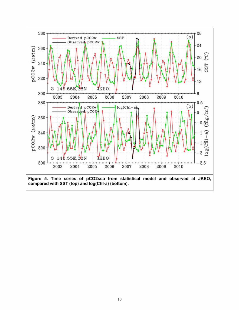
Figures 4 and 5 show that our output agrees well with in situ measurements, two years at KEO and one year at JKEO, that were accessible to us. Our data show year-to-year variation. At KEO to the south (Fig. 4), the annual variations of pCO2sea agree well with SST, but they do not follow the semi-annual variations of Chl-a. At JKEO to the north, there are two cycles a year in opposite phase with Chl-a, but SST has only one cycle per year.

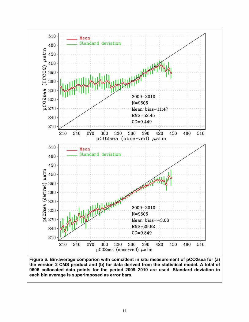
9. Comparison with CMS product The current JPL CMS bottom-up flux estimate is a model-based (http://cmsflux.jpl.nasa.gov) effort to compute pCO2sea by combining the Estimating the Circulation and Climate of the Ocean Phase II (ECCO2) model (Marshall et al. 1997), which provides the time-evolving physical ocean state, and the Darwin model (Follows and Dutkiewicz 2011), which provides time-evolving ocean ecosystem variables. CMS produced a comparison of the two years of data (2009 and 2010) with coincident LDEO in situ measurement, as shown in Fig 7 of Brix et al. (2012). The scatter is very large, for the high temporal resolution data, but generally around the central line. The more obvious problem is at low observed values (below 320 ppm), where a large number of over-estimations (above 370 ppm) are found. The LDEO data are a subset of the in-situ data we collected as discussed in Section 5. A similar comparison with our data is provided in Fig. 6.

The 2 years of data over the global ocean provided by CMS are collocated with our products and in-situ measurements. Figure 6 shows the results of the comparisons in the form of a bin-averaged scatterplot of 9606 daily data pairs. The lack of sensitivity of CMS product at low values is obvious in Fig. 6a, and this is in agreement with the overestimation at low values shown by Brix et al. (2012). Our products at the same locations and times show better agreement with the in-situ data, as shown in Fig. 6b. The root-mean-square (RMS) difference with in situ measurement is 52.45 μatm for CMS product, higher than 29.82 μatm for our product. The correlation coefficient of 0.45 for CMS is lower than the 0.85 for our product.

The geographic distribution of the 2-year averages of our products (Fig. 7a) agree with Takahashi climatology (Fig 7c) better than CMS product (Fig. 7b). The overestimation (lack of sensitivity) of CMS products is found largely over the oligotrophic subtropical oceans, and this suggests that the Darwin model may be deficient where ocean biological productivity is not a significant driver of surface carbon fugacity, as demonstrated in Section 8.

8

Figure 3 Latitudinal-time variabilition along 148°E in North Pacific: (a) pCO2sea derived from Takahashi et al. (2013) climatology data; (b) same as (a), but from statistical model using satellite data, averaged over the 2003–2010 period; (c) and (d) the same as (b), except for log(Chl-a) and SST, respectively;(e) Location of two stations and the 148° E longitude line.

9

Figure 4. Time series of pCO2sea from statistical model and observed at KEO, compared with SST (top) and log(Chl-a) (bottom).

10

Figure 5. Time series of pCO2sea from statistical model and observed at JKEO, compared with SST (top) and log(Chl-a) (bottom).

11

Figure 6. Bin-average comparion with coincident in situ measurement of pCO2sea for (a) the version 2 CMS product and (b) for data derived from the statistical model. A total of 9606 collocated data points for the period 2009–2010 are used. Standard deviation in each bin average is superimposed as error bars.

12

Figure 7. Distribution of pCO2sea (a) derived from satellite data using the statistical model, averaged for period 2009-2010. (b) same as (a), except from the version 2 of CMS products. (c) same as (b), except from Takahashi et al. (2012) climatological data.

13

10. Future Work The current data will be distributed through website http://airsea.jpl.nasa.lgov/seaflux. It is a living data set. The model will be changed as more data with better coverage become available. It will extend, as new satellite sensors replace the old. For example, AMSR-2 on Global Change Observation Mission 1-Water (GCOM-W) has replaced AMSR-E.

Aquarius is a satellite mission to measure sea surface salinity (SSS), which was launched in 2011 and covers Earth's surface once every 7 days. The SSS data have 1º resolution. Soil Moisture and Ocean Salinity (SMOS), launched in November 2009, is also providing global SSS measurements with 3 days revisits. Intercalibration and merging of SST products are conducted and coordinated by the Group for High Resolution Sea Surface Temperature (GHRSST) Project. We will use these products to extend the time series, when funding support becomes available.

11. References

Behringer, D. W., 2007: The Global Ocean Data Assimilation System (GODAS) at NCEP. Preprints, 11th Symp. on Integrated Observing and Assimilation Systems for Atmosphere, Oceans, and Land Surface, San Antonio, TX, Amer. Meteor. Soc., 3.3. [Available online at http://ams.confex.com/ams/87ANNUAL/techprogram/paper_119541.htm.]

Bogucki, D., M.-E. Carr, W.M. Drennan, P. Woicesyn, T. Hara, and M. Schmeltz, 2010: Preliminary and novel estimates of CO2 gas transfer using a satellite scatterometer during the 2001 GasEx experiment. Int. J. Remote Sensing, 31, 75–92.

Boutin, J., J. Etcheto, L. Merlivat, and Y. Rangama, 2002: Influence of gas exchange coefficient parameterisation on seasonal and regional variability of CO2 air-sea fluxes, Geophys. Res. Lett., 29(8), 1182, doi:10.1029/2001GL013872.

Boyer, T., S. Levitus, H. Garcia, R. A. Locarnini, C. Stephens, J. Antonov, 2005: Objective analyses of annual, seasonal, and monthly temperature and salinity for the world ocean on a 0.25 degree grid. Int. J. Clim., 25, 931–945.

Brix, H., D. Menemenlis, C. Hill, S. Dutkiewicz. O. Jahn, D. Wang, K. Bowman, and H. Zhang, 2012: Using Green’s function to initialize and adjust a global, eddy ocean biogeochemistry general circulation model. Submitted to Ocean Modelling

Canadell J. G., Le Quéré C., Raupach M. R., Field C. B., Buitenhuis E. T., Ciais P., Conway T. J., et al., 2007: Contributions to accelerating atmospheric CO2 growth from economic activity, carbon intensity, and efficiency of natural sinks. Proceedings of the National Academy of Sciences. doi: 10.1073/pnas.0702737104.

Carr, M. E., W. Tang, and W. T. Liu, 2002: CO2 exchange coefficients from remotely sensed wind speed measurements: SSM/I versus QuikSCAT in 2000. Geophys. Res. Lett., 29 (15), doi:10.1029/2002GL015068.

Chevallier F., R. J. Engelen, and P. Peylin: 2005: The contribution of AIRS data to the estimation of CO2 sources and sinks. Geophys. Res. Lett., 32, L23801, doi:10.1029/2005GL024229.

Cosca, C. E., R. A. Feely, J. Boutin, J. Etcheto, M. J. McPhaden, F. P. Chavez, and P. G. Strutton, 2003: Seasonal and interannual CO2 fluxes for the central and eastern equatorial Pacific Ocean as determined from fCO2-SST relationships. J. Geophys. Res., 108(C8), 3278, doi:10.1029/2000JC000677.

14

Crisp, D., R. M. Atlas, F.-M. Breon, L. R. Brown, J.P. Burrows, P. Ciais, B. J. Connor, S. C. Doney, I. Y. Fung, D. J. Jacob, C. E. Miller, D. O’Brien, S. Pawson, J. T. Randerson, P. Rayner, R. J. Salawitch, S. P. Sander, B. Sen, G. L. Stephens, P. P. Tans, G. C. Toon, P. O. Wennberg, S. C. Wofsy, Y. L. Yung, Z. Kuang , B. Chudasama, G. Sprague, B. Weiss, R. Pollock, D. Kenyon, and S. Schroll, 2004: The Orbiting Carbon Observatory (OCO) mission, Advances in Space Research, 34, 700–709.

Dickson, A. G., Sabine, C. L. and Christian, J. R. (Eds.) 2007: Guide to Best Practices for Ocean CO2 Measurements. PICES Special Publication, 3, 191 pp. http://cdiac.ornl.gov/ftp/oceans/Handbook_2007/Guide_all_in_one.pdf

DOE 1994: Handbook of methods for the analysis of the various parameters of the carbon dioxide system in sea water; version 2, A.G. Dickson, and C. Goyet, Eds. ORNL/CDIAC-74.

Engelen, R. J., S. Serrar, and F. Chevallier, 2009: Four-dimensional data assimilation of atmospheric CO2 using AIRS observations, J. Geophys. Res., 114, D03303, doi:10.1029/2008JD010739Follows, M.J. and S. Dutkiewicz, 2011: Modeling diverse communities of marine microbes, Annual Reviews of Marine Science, 3, 427–451.

Frew, N., 1997: The role of organic films in air-sea gas exchange, Eds. P.S. Liss and R.A. Duce, The sea surface and global change, 121–172. Cambridge Univ. Press, New York.

Friedrich, T., and A. Oschlies, 2009: Basin-scale pCO2 maps estimated from ARGO float data – a model study. J. Geophys. Res., 114, C10012, doi:10.1029/2009JC005322.

Glover, D. M., N. M. Frew, S. J. McCue and E. J. Bock, 2002: A multi-year time series of global gas transfer velocity from the Topex dual frequency, normalized radar backscatter algorithm. In: Donelan, M. A., W. M. Drennan, E. S. Saltsman and R. Wanninkhof, Editors, Gas Transfer at Water Surfaces, Geophysical Monograph, vol. 127, American Geophysical Union, Washington, DC, 325–331.

Goyet, C., Millero, F. J., O'Sullivan, D.W., Eischeid, G., McCue, S. J. and Bellerby, R. G. J., 1998: Temporal variations of pCO2 in surface seawater of the Arabian Sea in 1995. Deep-Sea Research I, 45, 609–623.

Gurney, K. R., et al., 2004: Transcom 3 inversion intercomparison: Model mean results for the estimation of seasonal carbon sources and sinks. Global Biogeochem. Cycles, 18, GB1010, doi:10.1029/2003GB002111.

Hashizume, H. and W. T. Liu, 2004: Systematic error of microwave scatterometer wind related to the basin scale plankton bloom. Geophys. Res. Lett., 31, L06307, doi:10.1029/2003GTL01841.

Hein, R., P. J. Crutzen, and M. Heimann, 1996: An inverse modeling approach to investigate the global atmospheric methane cycle. Global Biogeochemical Cycles, 11, 43–76.

Hood, E. M., L. Merlivat, and T. Johannessen, 1999: Variations of fCO2 and air–sea flux of CO2 in the Greenland Sea gyre using high-frequency time series data from CARIOCA drift buoys. Journal of Geophysical Research, 104, 20571–20583.

Hoffmann, D. J., J. H. Butler, and P. Tans, 2009: A new look at atmospheric carbon dioxide. Atmos. Envir., 43, 2084.

Key, R. M., T. Tanhua, A. Olsen, M. Hoppema, S. Jutterström, C. Schirnick, S. van Heuven, A. Kozyr, X. Lin, A. Velo, D. Wallace and L. Mintrop. 2010: The CARINA data synthesis project: Introduction and overview. Earth System Science Data, 2(1), 105–121.

Le Quéré, C., C. Rödenbeck, E.T. Buitenhuis, T. J. Conway, R. Langenfelds, A. Gomez, C. Labuschagne, M. Ramonet, T. Nakazawa, N. Metzl, N. Gillett, and M. Heimann, 2007: Saturation of the Southern ocean CO2 sink due to recent climate change. Science, 316, DOI:10.1126/science.1136188, 1735–1738.

15

Lefevre, N., A. J. Watson, and A. R. Watson, 2005: A comparison of multiple regression and neural network techniques for mapping in situ pCO2 data. Tellus B, 57, 375–384. doi: 10.1111/j.1600-0889.2005.00164.x.

Lewis, E., and D. W. R. Wallace, 1998: Program Developed for CO2 System Calculations. ORNL/CDIAC-105. Carbon Dioxide Information Analysis Center, Oak Ridge National Laboratory, U.S. Department of Energy, Oak Ridge, Tennessee.

Lin, I-I, W. Alpers, and W.T. Liu, 2003: First evidence for the detection of natural surface films by the scatterometer. Geophys. Res. Lett., 30(13), 1713, doi:10.1029/2003GL017415.

Liss P.S., and L. Merlivat, 1986: Air-sea gas exchange rates: Introduction and synthesis. In: P. Buat-Ménart, Editor, The Role of Air-Sea Exchange in Geochemical Cycling, D. Reidel Pub Co, Dordrecht, Netherlands, 113–127.

Liu, W. T., X. Xie, and W. Tang, 2010: Scatterometer’s unique capability in measuring ocean surface stress. Oceanography from Space, Barale, Gower, and Alberotanza (eds), Springer, 93–111.

Marshall, J., A. Adcroft, C. Hill, L. Perelman, and C. Heisey, 1997: A finite-volume, incompressible Navier-Stokes model for studies of the ocean on parallel computers, J. Geophys. Res., 102 (C3), 5753–5766.

Nelson, N.B., N.R. Bates, D. A. Siegel, A.F. Michaels, 2001: Spatial variability of the CO2 sink in the Sargasso Sea. Deep-Sea Research II 48, 1801-1821.

Nightingale, P., Malin, G., Law, C., Watson, A., Liss, P., Liddicoat, M., Boutin, J., and Upstill-Goddard, R., 2000: In situ evaluation of air-sea exchange parameterizations using novel conservative and volatile tracers. Glob. Biogeochem. Cycles, 14, 373–387.

Ono, T., T. Saino, N. Kurita, and K. Sasaki, 2004: Basin-scale extrapolation of shipboard pCO2 data by using satellite SST and Chla'. International Journal of Remote Sensing, 25(19), 3803–3815.

Padin X. A., G. Navarro, M. Gilcoto, A. F. Rios, F. F. Perez, 2009: Estimation of air-sea CO2 fluxes in the Bay of Biscay based on empirical relationships and remotely sensed observations. J. Marine Systems, 75, 280–289.

Patra, P. K., et al., 2006: Sensitivity of inverse estimation of annual mean CO2 sources and sinks to ocean-only sites versus all-sites observational networks, Geophys. Res. Lett., 33, L05814,

Pfeil, B., Olsen, A., Bakker, D. C.E. et al., 2013: A uniform, quality controlled Surface Ocean CO2 Atlas (SOCAT), Earth Syst. Sci. Data, 5, 125-143, doi:10.5194/essd-5-125-2013.

Pierrot, D., P. Brown, S. van Heuven, T. Tanhua, U. Schuster, R. Wanninkhof, and R. Key, 2010: CARINA TCO2 data in the Atlantic Ocean. Earth Syst. Sci. Data, 3, 1–26.

Sarma, V. V. S. S., T. Saino, K. Sasaoka, Y. Nojiri, T. Ono, M. Ishii, H. Y. Inoue, and K. Matsumoto, 2006: Basin-scale pCO2 distribution using satellite sea surface temperature, Chl a, and climatological salinity in the North Pacific in spring and summer. Global Biogeochem. Cycles, 20, GB3005, doi:10.1029/2005GB002594.

Smola, A. J., and B. Schölkopf, 2004: A tutorial on support vector regression. Statistics and Computing, 14, 199–222.

Stephens, M. P., G. Samuels, D. B. Olson, R. A. Fine, and T. Takahashi. 1995: Sea-air flux of CO2 in the North Pacific using shipboard and satellite data. J. Geophys. Res., 100, 13571–13583.

Takahashi, T., S. C. Sutherland, C. Sweeney, A. Poisson, N. Metzl, B. Tillbrook, N. Bates, R. Wanninkhof, R. A. Feely, C. Sabine, J. Olafsson, and Y. Nojiri, 2002: Global sea-air CO2 flux based on climatological surface ocean pCO2, and seasonal biological and temperature effects, Deep-Sea Res. II, 49, 1601–1622.

16

Takahashi, T., S. C. Sutherland, and A. Kozyr. 2013. Global Ocean Surface Water Partial Pressure of CO2 Database: Measurements Performed During 1957-2012 (Version 2012). ORNL/CDIAC-160, NDP-088(V2012). Carbon Dioxide Information Analysis Center, Oak Ridge National Laboratory, U.S. Department of Energy, Oak Ridge, Tennessee, doi: 10.3334/CDIAC/OTG.NDP088(V2012).

Telszewski, M., A. Chazottes, U. Schuster, A. J. Watson, C. Moulin, D. C. E. Bakker, M. González-Dávila, T. Johannessen, A. Körtzinger, H. Lüger, A. Olsen, A. Omar, X. A. Padin, A. Ríos, T. Steinhoff, M. Santana-Casiano, D. W. R. Wallace, and R. Wanninkhof, 2009: Estimating the monthly pCO2 distribution in the North Atlantic using a self-organizing neural network, Biogeosciences Discuss., 6, 3373-3414, doi:10.5194/bgd-6-3373–2009.

Tsai, W.-T., and L.-Y. Liu, 2004: Transport of exogenous surfactants on a thin viscous film within an axisymmetric airway. Colloids and Surfaces A, 234(1-3), 51–62

Wanninkhof, R., 1992: Relationship between wind speed and gas exchange over the ocean. J. Geophys. Res., 97, 7373–7382.

Watson, A. J., C. Robinson, J.E. Robinson, P. J. le.B. Williams, and M. J. R. Fasham, 1991: Spatial variability in the sink for atmospheric carbon dioxide in the North Atlantic. Nature, 350, 50–53.

Watson, A. J., U. Schuster, D. C. E. Bakker, N. Bates, A. Corbiere, M. Gonzalez-Davila, T. Friedrich, J. Hauck, C. Heinze, T. Johannessen, A. Kortzinger, N. Metz, J. Olaffson, A. Oschlies, B. Pfeil, A. Olsen, A. Oschlies, J. M. Santano-Casiano, T. Steinhoff, M. Telszewski, A. Rios, D. W. R. Wallace, R. Wanninkhof, 2009: Tracking the variable North Atlantic sink for atmospheric CO2. Science, 326, 1391–1393.

Weiss, R. F. 1974: Carbon dioxide in water and seawater: The solubility of a non-ideal gas. Marine Chemistry, 2, 203–215.

Wentz, F. J., and T. Meissner, 1999: AMSR Ocean Algorithm, Version 2. RSS Tech. Report 121599A, Remote Sensing Systems. Santa Rosa, CA.

Woolf, D. K., 1997: Bubbles and their role in gas exchange. In: P.S. Liss and R.A. Duce, Editors, The Sea Surface and Global Change, Cambridge University Press, Cambridge, UK, 173–205.

Xie X., W. T. Liu, and B. Tang, 2008: Spacebased estimation of moisture transport in marine atmosphere using support vector machine, Remote Sens. Environment, 112, 1846–1855.

Yang, Z., R. A. Washenfelder, G. Keppel-Aleks, N. Y. Krakauer, J. T. Randerson, P. P. Tans, C. Sweeney, and P. O. Wennberg, 2007: New constraints on Northern Hemispheric growing season net flux, Geophys. Res. Lett., 34, L12807, doi:10.1029/2007GL029742.

Zhu, Y., S. Shang, W. Zhai, and M. Dai, 2009: Satellite-derived surface water pCO2 and air–sea CO2 fluxes in the northern South China Sea in summer. Progress Nat. Sci., 19, 775–779.

12. Acronyms and Abbreviations α solubility of CO2 in seawater ΔT difference in time AMSR-E Advanced Microwave Scanning Radiometer for EOS AOML Atlantic Oceanographic and Meteorological Laboratory CARINA CARbon dioxide IN the Atlantic Ocean

17

CDIAC Carbon Dioxide Information Analysis Center Chl-a chlorophyll a CLIVAR Climate Variability Program CMS (Jet Propulsion Laboratory) Carbon Monitoring System CO2 carbon dioxide DIC dissolved inorganic carbon ECCO2 Estimating the Circulation and Climate of the Ocean Phase II (model) EOS Earth Observing System f fugacity F air-sea exchange in Co2

GCOM-W Global Change Observation Mission 1-Water GHRSST Group for High Resolution Sea Surface Temperature GLODAP GLobal Ocean Data Analysis Project GODAS Global Ocean Data Assimilation System JKEO Japan Agency for Marine-Earth Science and Technology (JAMSTEC) Kuroshio

Extension Observatory [The definition came from JGR at http://www.pmel.noaa.gov/people/cronin/articles/TomitaetalJGR10a.pdf

JPL Jet Propulsion Laboratory k CO2 gas transfer (piston) velocity KEO Kuroshio Extension Observatory LDEO Lamont–Doherty Earth Observatory MLD mixed layer depth OCO Orbiting Carbon Observatory p pressure PACIFICA PACIFic ocean Interior CArbon PICES North Pacific Marine Science Organisation [British spelling] PMEL Pacific Marine Environmental Laboratory

18

RMS root mean square SeaWiFs Sea-viewing Wide Field-of-view Sensor SMOS Soil Moisture and Ocean Salinity SOCAT Surface Ocean CO2 Atlas SSS sea surface salinity SST sea surface temperature SVM support vector machine SVM support vector machine used for regression TCO2 total dissolved inorganic carbon VOS Volunteer Observing Ship (project)