oes protection beget corruption pushan dutt … · the trade literature has addressed this issue...

DOES PROTECTION BEGET CORRUPTION?*

Pushan Dutt Department of Economics

7-11 Tory, University of Alberta Edmonton, AB T6G 2H4

[email protected] July 22, 2002

Abstract

This paper develops and tests a model, which predicts that protectionist policies on the part of the government leads to increased corruption on part of the bureaucracy. A one-sector small open economy model is presented. Corruption is shown to be increasing in tariffs and subsidies, and decreasing in civil sector wages. Using multiple measures of corruption and protection, the predictions of the model are tested. We find evidence suggesting that corruption is indeed higher in countries pursuing active trade and industrial policies. The empirical results are checked for robustness and policy implications are discussed. Key Words: Corruption, Protection JEL Codes: F10, F13, F14, D72, D73

* I would like to thank Andres Velasco, Raquel Fernandez, Giovanni Maggi, Giorgio Topa, Debraj Ray and Devashish Mitra for invaluable suggestions and comments. I thank seminar participants at New York University, University of Alberta, University of Georgia and the Southeast International Economics Conference for very useful discussions. I would also like to thank Francesco Rodriguez, Daniel Lederman, Paulo Mauro, Caroline Van Rijckeghem and Beatrice Weder for sharing their data with me. The usual disclaimer applies.

1 Introduction

Are countries that are more protectionist also more corrupt? The paper addresses this question,

first within a theoretical framework that delineates the channels through which protectionist

trade policies affect corruption. It then verifies the model predictions empirically. Traditionally,

a number of arguments have been advanced to justify trade protection: (i) The terms of trade

argument - this requires that a country possess some degree of market power in world markets.

(ii) Strategic trade policy arguments - in the presence of strategic interactions, governments can

use appropriate policies (tariffs or subsidies) to shift rents from foreign to domestic firms. (iii)

The production efficiency effect - protection can induce, under some circumstances, an increase

in domestic production and improve welfare. (iv) The external economies argument - the most

popular version is the infant industry argument widely cited by policy makers in developing

nations in the post World War period. (v) Factor market distortions provide another justification

for trade policies. All such arguments sketch a variety of scenarios where trade protection can

enhance welfare.

The purpose of this paper is not to take up any particular position on the relative merits of

free trade vs. protectionism. Rather, it is to point to a side effect of trade protection that could

temper or even compromise the goals of trade policy. We show that activist trade and industrial

policies lead to an increase in corrupt activities on the part of the bureaucracy. In particular,

trade and subsidy protection transfer rents to firms, and bureaucrats who we assume, control the

rights to licensing of production, extract these rents from firms in the form of bribes. If we believe

that protectionist policies are welfare enhancing, the calculus of such policy needs to factor the

effect of corruption that such policies generate and which, in turn, can be welfare reducing.1 In a

nutshell, there exists a trade off between the direct welfare enhancing effects of trade and industrial

policies and their indirect welfare reducing effects operating through the channel of corruption.

1 Mauro (1995) for instance, shows that corruption has a negative impact upon economic growth.

1

The trade literature has addressed this issue briefly in the form of the Krueger’s (1974) analysis

of rent seeking activities.2 She recognizes that government regulations are pervasive, and give

rise to rents and rent-seeking, which may take the form of bribery and corruption. However, her

analysis is mainly concerned with showing that welfare losses with import quotas (that give rise

to rent-seeking) are greater than losses under an equivalent tariff. This paper focuses on the fact

that any of a plethora of trade restrictions can transfer rents to domestic firms and provide greater

incentives to the bureaucrats at the margin to be corrupt.

While corruption has recently attracted increasing attention,3 empirical studies on the factors

that promote corruption are limited. A majority of the studies, such as Becker and Stigler (1975),

Rose-Ackerman (1975), and Klitgaard (1988, 1990), analyze bureaucratic corruption as a principal-

agent problem. The focus is on devising ways and means that enforce honesty on part of the

bureaucrats. Others seek to explain the persistence of corruption in terms of frequency dependent

models that generate multiple equilibria. Lui (1986), Cadot (1987), and Andvig and Moene (1990)

present models in this vein. Another stream of research analyzes the consequences of governmental

corruption. Mauro (1995) looks at the effect of corruption on investment and growth; Wei (1997)

analyzes its impact on foreign direct investment and Mauro (1998) examines whether corruption

distorts the composition of government expenditure.

To the best of the author’s knowledge there exist a handful of papers that try to explain cross-

country variations in corruption. Ades and Di Tella (1997), show that corruption is associated

with active industrial policies and Van Rijckeghem and Weder (1997) show that there is a negative

relationship between corruption and civil sector wages. While the former concentrates purely on

industrial policies in terms of examining the effects of favorable domestic procurement and fiscal

policies on corruption, the latter concentrates on testing efficiency wage models of corruption. Nei-

ther paper examines the effect of trade policies and both test their models only for a small sample

2 See also Bhagwati (1982) for a general concept of directly unproductive activities and the welfare consequencesof such activities.

3 See Bardhan(1997) for a useful survey.

2

of countries (32 countries in Ades and Di Tella and 25 developing countries in Van Rijckeghem and

Weder). More recently, Treisman (2000) finds that countries with Protestant traditions, histories

of British rule, more developed economies, and higher imports were less corrupt. Ades and Di

Tella (1999) focus on how competition affects corruption and find empirically that rents, proxied

by lack of import competition, fuel and mineral exports, and trade distance, increase corruption.

However, none of these papers systematically investigate the effect of activist trade policies upon

corruption.4 This paper, while emphasizing the effect of protectionist policies on corruption, also

attempts to explain differences in corruption levels across a broad cross-section of countries. Ac-

cordingly, this paper identifies the channels through which corruption operates, the inducements

for bureaucrats to engage in dishonest behavior, and the various checks on such malfeasant behav-

ior. It then proceeds to test whether the empirical counterparts to these explanatory variables,

do in fact, explain the cross-sectional variation in levels of corruption.

We set up a simple small open economy model within which corruption and bribes are deter-

mined. Corruption in this model takes the form of petty bureaucratic corruption. The bureaucrats

are the agents of the government and are entrusted with carrying out a task by the government

but engages in malfeasance that is difficult to monitor. Bribes take the form of a price for license

(whose market price is set to zero, viz., there are no licensing fees), and corruption manifests itself

in the form of a transfer of surplus from firm owners to bureaucrats. Bribes are assumed to be

determined via a bargaining process between the bureaucrat and the firm. We assume that the de-

tection probability and the wages of bureaucrats are exogenously given, thereby abstracting from

issues of multiple equilibria and the design of incentive compatibility contracts by the government

to deter corruption. In our model we show that a larger surplus provides greater inducement to be

corrupt, and protectionist policies add to the surplus earned by domestic firms. The model, thus

predicts that trade and industrial policies lead to higher bribes and a greater incidence of corrup-

4 Most empirical papers on the determinants of corruption throw in³X+MGDP

´or M

GDPas a control for openness.

However, this is an indirect measure of trade restrictions and notoriously unreliable.

3

tion. In the model, corruption results arises out of the interaction of the discretionary power of the

bureaucrats and from the monopoly power enjoyed by firms. Corruption indices from a variety of

survey measures, is regressed upon a variety of measures of trade and industrial policy, licensing

regulations, proxies for the detection probability, civil sector wages and relevant controls. We find

strong support that protectionism engenders corruption - a result which is robust to the treatment

of corruption as an ordinal measure, to endogeneity issues, and to variations in corruption over

time and space.

The paper is organized as follows. Section 2 sets out the model; Section 3 solves for the

equilibrium and performs some comparative statics; Section 4 lists the data sources and provides

descriptive statistics for the variables to be used in the empirical analysis; Section 5 discusses the

empirical findings; Section 6 concludes.

2 The Model

2.1 The Consumer and Firm’s Problem

This section develops a basic monopolistic competition model with differentiated products and

intra-industry trade. Consider a small open economy model where following convention, we label

the two countries as ‘Home’ and ‘Foreign’ with the analysis being confined to the home country

and where the label ’Foreign’ will be reinterpreted to mean the rest of the world.5

It is assumed that there are a continuum of differentiated products, each produced under in-

creasing returns to scale by a monopolist for that particular variety. The representative individual

has a Dixit-Stiglitz constant elasticity utility function,

U =

ÃZ n

0

xσ−1σ

hi di+

Z n∗

0

xσ−1σ

fi di

! σσ−1

, σ > 1 (1)

where xhi is the consumption of the domestically produced variety i and xfi is the consumption of

the imported variety i. n and n∗ are the total number of domestic varieties and foreign varieties

5 In a two country framework, the analysis will remain unchanged.

4

respectively, and σ is the elasticity of substitution. This structure yields the following domestic

demand functions for the differentiated products.6

xhi =³phiP

´−σ EP; xfi =

³pfiP

´−σ EP

(2)

where E is the country’s total spending which we assume to equal its income, phi is the consumer

price of the domestically produced variety, pfi is the domestic consumer price of the imported

variety and

P =

ÃZ n

0

p1−σhi di+

Z n∗

0

p1−σfi di

! 11−σ

(3)

is an index of the prices of the differentiated goods. Foreign demand for domestic varieties is

derived in an analogous manner

x∗hi =µp∗hiP ∗

¶−σE∗

P ∗(4)

where E∗ is the foreign spending and income, p∗hi is the foreign consumer price of the variety i

produced at home and

P ∗ =

ÃZ n

0

p∗1−σhi di+

Z n∗

0

p∗1−σfi di

! 11−σ

Under the small open economy assumption, the country faces a given foreign price and a given

number of the differentiated products, and a given foreign spending on differentiated products.

The small open economy imposes a tariff t on the imports of differentiated products. This implies:

pfi = (1 + t)p∗fi

where p∗fi is the foreign price of the foreign variety i. Despite the small open economy assumption,

domestic firms posess monopoly power and face a downward sloping demand schedule. We further

assume that the home country provides export subsidies at the rate e on home differentiated goods

so that

p∗hi =phi

(1 + e)

6 ∗ denotes the variable refers to price or demand in the foreign country and the subscript, h, f denotes whetherthe good in question is of the home country or foreign country.

5

We also assume that foreign varieties are equally priced with units conveniently chosen so that

p∗fi = 1, ∀i. The above price relationships imply

xhi =³phiP

´−σ EP; xfi =

µp∗fi(1 + t)

P

¶−σE

P; x∗hi =

Ãphi(1+e)

P ∗

!−σE∗

P ∗(5)

P =

µZ n

0

p1−σhi di+ n∗ [1 + t]1−σ¶ 1

1−σ; P ∗ =

ÃZ n

0

µphi1 + e

¶1−σdi+ n∗

! 11−σ

(6)

The home producer of variety i faces the demand function of xhi + x∗hi. Given the continuum

of varieties each producer is negligible with respect to the entire market and therefore faces a

constant elasticity of demand, σ.

We now assume that there are two factors of production in fixed supply: unskilled labor that

we denote as L and ’entrepreneurs’ whom we denote as K̇. Entrepreneurs provide managerial

and organizational skills and we assume that 1 unit of ‘entrepreneurs’ is required to commence

production. Therefore, production has a constant unit labor requirement of c and a fixed cost of 1

unit of ’entrepreneurs’. The latter is independent of the quantity produced. wh is the remuneration

to the entrepreneur and w is the wage of unskilled labor. w is chosen as the numeraire with units

chosen such that w = 1. Firms engage in monopolistic competition and obtain an output subsidy

at the rate of s per unit produced. Total costs of producing x units of a variety is therefore

wh + wcx− sx = wh + (c− s)x (7)

The pricing rule derived from profit maximization is

phi = pi =σ

σ − 1(c− s) (8)

which implies that all home varieties are equally priced with pi = p and produced in the same

quantity, xhi + x∗hi = xh + x

∗h = x. The fixed endowment of entrepreneurs, K determines, n = K

as the number of varieties. Finally, the wages of the entrepreneur is simply the profit or surplus

left over after payment to unskilled labor. Therefore wh must satisfy

wh = px− (c− s)x (9)

6

There are L units of unskilled labor each of whom earn w = 1 and K entrepreneurs each of whom

earn wh. National income is therefore given as

Y = E = L+ whK + T (10)

where T is the net rebate from the government’s policy. We assume that subsidies are financed

and tariffs are rebated by the government in a lump sum fashion. The government also pays the

wages of bureaucrats wb who are of measure 1. Therefore, the budget constraint of the government

is as follows

wb + eKp∗hx∗h + sK(x

∗h + xh) + T = tn

∗p∗xf (11)

where wb is the wage of each bureaucrat. T adjusts so that the above equality always holds.

Lemma 1 In the profit maximizing equilibrium, a small increase in the tariff rate t, in the exportsubsidy s, or in the output subsidy e, raises the wages or the operating surplus of the entrepreneur..

Proof: Operating surplus can be written as

wh = (p− c+ s)x

By the envelope theorem

∂wh∂s

= x > 0

Total revenue may written using equations (6)-(9) as

px = p(xhi + x∗hi)

=p1−σ

np1−σ + n∗(1 + t)1−σY + (1 + e)

hp1+e

i1−σnh

p1+e

i1−σ+ n∗

E∗

Now profits may be written as a constant share of revenue using the mark-up pricing equation.

That is

wh =px

σ

Since σ > 1, from the above equations it follows that

∂wh∂t

> 0

∂wh∂e

> 0

7

Therefore, within this framework any form of government intervention serves to increase the return

to the skilled factor owner or the entrepreneur7 .

2.2 The Bureaucrat’s Problem

Each entrepreneur in order to commence production has to obtain a license from the government.

Licenses are approved by bureaucrats who act as agents of the government, thereby providing them

with discretionary power. There are a continuum of bureaucrats over the interval [0, 1] and every

entrepreneur is matched at random with a particular bureaucrat. Licenses are assumed to be cost-

less. Bureaucrats might, however, choose to be corrupt and demand bribes from the entrepreneur

in return for issuing the license. In case they choose to demand a bribe, the bribe amount is

determined through a Nash bargaining game between the bureaucrat and the entrepreneur.

Each bureaucrat faces a two stage decision problem: in stage 1 they choose whether to be

honest or to be corrupt, in stage 2 they choose the bribe conditional on the decision in stage 1. Of

course, if they choose to be honest they set the bribe to zero in stage 2. Bureaucrats are assumed

to be risk neutral and maximize their expected income from corruption.

Stage 1 : In stage 1 bureaucrats choose between being ‘honest’ or being ‘corrupt’. If they are

honest they merely receive their wages wb which is assumed to be exogenously given. If they

choose to be corrupt, then their income consists of their wage income wb and bribe income, b so

that their total income from corruption equals wb+ b. However, there is an exogenous determined

probability of being caught β(b) in corrupt transactions, in which case they are simply fired and

lose both their wage as well as bribe income. With probability (1− β(b)) they are not caught so

that the expected income from being corrupt equals (1−β(b))(wb+b)+β(b)·0 = (1−β(b))(wb+b).

We assume that

β(b) =

0 for b = 0

β for b > 0

(12)

7 Given that entrepreneurs also consume the differentiated goods, subsidies are simply a transfer from consumers(who are presumably taxed in a lumpsum fashion) to entrepreneurs so that Y is unaffected. Tariffs on the otherhand generate tariff revenues which is repatriated to consumers so Y would increase.

8

This assumption implies that every bureaucrat who chooses to be corrupt and sets b = 0 in effect

chooses to be honest.

In addition, we assume that bureaucrats have certain moral costs from being corrupt and these

moral costs, denoted as ci for the ith bureaucrat, are heterogenous across bureaucrats. These costs

are distributed over the interval [0, c∗] with the cumulative density F (c) such that F (0) = 0 and

F (c∗) = 1. Income and costs are measured in terms of the numeraire. Therefore, bureaucrat i

will choose to be corrupt as long as

ci < (wb + b) (1− β)− wb (13)

= b(1− β)− βwb (14)

Since bureaucrats are identical in all other respects, conditional on choosing to be corrupt they all

demand the same proportion g as bribes. This implies that the proportion of corrupt bureaucrats

or the incidence of corruption, given the values of β, g, wb and wh equals

γ =

F (max(0, (b(1− β)− βwb)) if c

∗ > (b(1− β)− βwb)

1 otherwise

(15)

The assumption that

c∗ > (wh(1− β)− βwb)

is sufficient to guarantee that γ = 1 cannot be an equilibrium. A low enough wb and β and a high

enough wh will guarantee that in equilibrium

b(1− β)− βwb > 0

so that γ = F (b(1− β)− βwb) > 0.8

Stage 2 : In this stage bureaucrats, conditional on choosing to be corrupt, choose b - the

bribe that they will demand which will come out of the entrepreneur’s operating surplus. The

bribe amount originates as a Nash bargaining exercise between the corrupt bureaucrat and the

8 Note that if the government could freely choose either wb or β it could ensure that γ = 0. However, budgetconstraints may prevent it from enforcing a zero corruption outcome.

9

entrepreneur. The disagreement point in this exercise is (0, 0), i.e., if there is no agreement, the

bureaucrat receives no payment as bribe, and the entrepreneur is who is denied the license cannot

commence production and therefore earns zero surplus.9 The entrepreneur and the bureaucrat

are both assumed to be risk neutral. Under the assumption of symmetrical bargaining power, the

equilibrium level of the bribe is determined as the solution to

argmaxb[b (wh − b)]

The Nash bargaining solution is

b =wh2

(16)

With asymmetric bargaining powers, bribes will continue to be a fraction of the surplus and

therefore increasing in the surplus.10 Therefore, we have the following lemma.

Lemma 2 The proportion of operating surplus demanded as bribe by the bureaucrat is increasingin the operating surplus.

In order to find the incidence of corruption, we solve the bureaucrat’s problem backwards.

Stage 2 gives b = wh2 which we use to obtain an expression for corruption as

γ = F³max

h0,wh2(1− β)− wbβ

i´if c∗ >

³wh2(1− β)− wbβ

´= 1 otherwise (17)

We will get an interior equilibrium with γ ∈ (0, 1) as long as 0 < wh2 (1− β)− wbβ < c∗ in which

case we may rewrite a simplified expression for γ.

γ = F³wh2(1− β)− wbβ

´Lemma 3 The incidence of corruption γ is increasing (weakly) in: (a) The operating surplus ofthe entrepreneur wh; and (b) weakly decreasing in the exogenously given detection probability βand in the wages of the bureaucrat wb

9 We could very well assume that the entrepreneur if denied the license, works as an unskilled worker and earnswages. This will not change any of the results. In this case the higher the wages of unskilled labor, the better isthe entrepreneur’s outside option, and thus lower will be corruption.

10 Here we set up the entreprenreur-bureaucrat interaction as a bargaining game. Alternatively, we could set itup as a non-cooperative game between the bureaucrats and entrepreneurs. The results remain unchanged.

10

Proof: Since F (.) is a cumulative density function it follows that

Fwh = F0́(.)(1− β)

2≥ 0

Fβ = F 0(.) ·³−wh2− wb

´≤ 0

Fwb = F 0(.) · (−β) ≤ 0

The weak inequality signs are used since γ may take the values 0 or 1. In the case of an interior

equilibrium, each of the signs above will be a strict inequality, provided F0́> 0.

3 The Equilibrium

We now try and determine the equilibrium levels of bribe and the operating surplus. Combining

Lemmas 1, 2 and 3 we can write the following proposition.

Proposition 4 The equilibrium level of the bribe g as a proportion of the surplus, and the inci-dence of corruption in equilibrium, γ is increasing in the import tariff t, the export subsidy s, andthe output subsidy s.

Proof:

With γ proportion of bureaucrats being corrupt. The entrepreneur will maximize her expected

income as

maxx

γ(wh − b) + (1− γ) (wh)

If the bureaucrat demands a proportion g as bribe so that b = gwh where g ∈ (0, 1) depends on

the bargaining power of the respective parties then, this is equivalent to maximizing

wh (1− γg)

Since γg < 1 the entrepreneur simply maximizes her operating surplus wh.Moreover, each corrupt

bureaucrat takes the operating surplus to be equal to this value and chooses whether to be corrupt

or honest to maximize her expected income. From Lemma 2 and 3, we have that

db

dwh> 0;

dγ

dwh≥ 0

11

Finally from Lemma 1 we have that the Nash level of the operating surplus is such that:

dwhdt

> 0,dwhde

> 0 anddwhds

> 0

Therefore

dg

dt> 0,

dg

de> 0 and

dg

ds> 0

and

dγ

dt≥ 0, dγ

de≥ 0 and dγ

ds≥ 0

The intuition behind this results is simple: greater protection yield greater rents or surplus to

the entrepreneurs thereby providing greater incentives for corruption. However, this is not the only

channel via which higher tariffs lead to a higher incidence of corruption. Where tariffs exist, there

is an incentive to evade them via smuggling, whether overt or in the form of invoicing changes.11

Both of these can manifest themselves in the form of corruption - the former as bribes paid to law

enforcement officials and the latter as bribes to customs officials. These incentives increase with

the tariff rate so that importers are willing to pay higher bribes as protection increases and this

will lead to higher corruption.

A second channel that may also lead to rent seeking and corruption, is tariff destroying lobbying

with the aid of bribes to politicians (See Bhagwati, 1982). Again, the higher the tariffs the higher

will be the willingness-to-pay of firms upon whom the tariff is imposed to reduce or remove the

tariff. Finally, as Bhagwati and Srinivasan (1980) point out, there may be a competition for

securing a share in the disbursement of tariff revenue. While they model the process as a legal

directly unproductive activity, the shares may be distributed in accordance to bribes paid by

various interest groups. This provides an additional channel through which protectionist policies

may impact corruption. Here, whether corruption is increasing in protectionist policies depends

crucially upon the elasticity of import demand.

11 Bhagwati and Hansen (1973), Bhagwati and Srinivasan (1973), Kemp (1976), Ray (1978) analyze smugglingas a directly unproductive activity and the relationship between commercial policy and smuggling.

12

4 Data Sources and Some Basic Statistics

Our dependent variable is corruption and our main independent variables are tariffs and subsidies.

In addition, we will be using independent variables that are likely to affect the detection probability

β, that control for alternative channels of corruption (in addition to tariffs and subsidies) and that

control for certain region specific effects. We will also use a variable that captures the level of

regulatory discretion present in the economy. It is the existence of such discretion from which

bureaucrats derive their power to extract rents.

We use three sources for data on the indices of corruption, all of which are based on surveys.

The first measure is the International Country Risk Guide (ICRG), available for 129 countries,

used previously and described in detail in Knack and Keefer (1993).12 Corruption is measured

on a zero to six scale, where low scores indicate high levels of corruption. The second measure

is compiled by Transparency International (TI). The TI index ranges from one (least corrupt) to

ten (most corrupt) and is itself an average of a number of survey results. The averaging procedure

should reduce measurement error if the errors in different surveys are independent. Table 2 in

the appendix shows the corruption ratings from Transparency International for 86 countries. We

use the 1998 TI index of corruption. Third, we use the German exporter corruption index (GCI)

which measures the total proportion of deals involving kickbacks, according to German exporters

(See Neumann (1994).13 To avoid awkwardness in the interpretation of the coefficients, the ICRG

and TI measures were recoded as six minus the original corruption index, and as ten minus the

original corruption index respectively, so that now higher numbers indicate higher corruption. As

shown in table 1.2, these three indices of corruption are highly correlated with the correlation

coefficient exceeding 0.8 for any pair of measures.

12 This measures the extent to which bribery is present “within the political system.” Forms of corruption givenin the ICRG are related to bribes in areas of exchange controls, tax assessments, police protection, loans andlicensing of exports and imports. Low scores on the corruption index indicate that ”government officials are likelyto demand special payments” and ”illegal payments are generally expected throughout lower levels of governmentin the form of bribes”.

13 This measure has the advantage of being an easily interpretable cardinal measure and accordingly we onlyreport OLS and IV results for this measure. However, data is available for only 43 countries.

13

To test for the robustness of our results, we use a variety of trade policy measures: total

import duties collected as a percentage of total imports (IMPORT DUTY), an average tariff

rate calculated by weighing each import category by the fraction of world trade in that category

(TARIFF),14 a coverage ratio for non-tariff barriers to trade (QUOTA). The last two measures,

tariffs and quotas are used in conjunction since they better capture trade restrictions when tariff

and non-tariff barriers are substitutes. We also use the Sachs-Warner openness indicator - an

indicator that attempts to solve the measurement error problem by constructing an index that

combines several aspects of trade policy. Although this is a coarse partition of economies into open

and closed economies, it will allow us to evaluate if the economies that are regarded as closed also

have a tendency to be more corrupt.15 For subsidies, there is very little cross-country data on

export subsidies. As a result, we are compelled to use a measure for subsidies obtained from the

World Development Indicators that measures all transfers from the Central government to private

and public enterprises as well as consumption subsidies.

We use two measures of civil sector wages from two different sources. First, a new data

set on civil sector wages has recently become available for 86 countries from the World Bank.

From here we use the real wage rate per government employee in constant 1997 dollars in our

analysis. The second wage concept used is the government wages relative to manufacturing wages.

Manufacturing wages may be thought as a proxy for outside option for bureaucrats (in case they

are caught taking bribes and fired) since the skill-content in the manufacturing sector is probably

lower than in the government sector, making it a suitable candidate for representing outside

opportunities for the bureaucrat. High manufacturing wages make corruption more attractive to

14 The variable is referred to as tariffs, although it includes all import charges, such as duties and customs fees.

15 The Sachs-Warner dummy takes the value of zero if the economy is closed according to any one of the followingcriteria: 1. Average tariff rates exceeded 40%; 2. Non-Tariff barriers covered more than 40% of imports; 3. Thecountry had a socialist economy system; 4. It had a state monopoly of major exports. 5. The black market premiumon the exchange rate exceeded 20% during either the 1970s or 1980s. This measure has been criticized on variousgrounds. For instance, the black market premia is more an indicator of macroeconomic imbalances and/or balanceof payment crisis. Further, as Rodrik and Rodriguez (1999) point out, the state monopoly of exports variableis virtually indistinguishable from a sub-Saharan African dummy because the World Bank study on the basis ofwhich it was constructed covered African countries that were under structural adjustment programs. Therefore,the empirical results that use the Sachs-Warner measure need to be interpreted with some caution.

14

bureaucrats as they become more willing to assume the risks of detection. This data is from van

Rijckeghem and Weder who have compiled this data for 28 developing over the period 1982-94.

We take the average relative wage for the 1980s. In addition, data for six OECD for exactly the

same variable was added from the OECD database.

The probability of detection cannot be observed directly so in its stead we use a number

of variables that we feel impact monitoring and through it the probability of detection. The

first variable that we use is democracy. Democratic countries are likely to exercise pressure

on politicians to keep corruption in check with the electorate punishing corrupt regimes at the

voting booth. A dictatorial regime on the other hand is likely to be less sensitive to demands for

controlling corruption through monitoring mechanisms and punishment schemes. For a measure

of democracy, we use the Freedom House measure of democracy, which derives from the work of

Gastil and his followers. The Gastil index provides a subjective classification of countries on a

scale of 1 to 7 on political rights, with higher ratings signifying less freedom. The average for

the 1980s is used. The other measures of checks that might affect the probability of detection

are schooling and the number of newspapers per thousand of the population. Both are likely to

increase the awareness of the public to illicit activities on part of the bureaucrat creating social

pressures against corruption. The fourth estate also acts as a guardian for the government and its

agents. The data on these measures are obtained from the World Development Indicators (2000).

A necessary condition for corruption to be present in the model is the existence of licensing.

This provides discretionary power to bureaucrats and thereby the ability to extract rents. More-

over, alternative channels could exist that promote corruption, such as distortion of wages and

prices through price controls. Therefore, we use two other variables - an index of regulation that

measures the degree to which licensing is prevalent in the economy and an index of wage and

price regulation. The former measures the degree of licensing requirements, as well as prevalent

levels of labor, environmental, consumer safety and worker health regulations. Wage and price

regulation, measures the degree to which the government controls wages and prices, through min-

15

imum wage laws and price controls. The data on these two measures is derived from the Heritage

Foundation, 1998. To control for regional effects we use three dummies: an East Asia dummy, an

oil dummy and a Sub-Saharan African dummy. Finally, in our instrumental variables estimation

we use ideology and ideology multiplied by the capital-labor ratio as instruments. The data on

political orientation are obtained from the Database of Political Institutions (DPI) (Beck et al,

2001) and measures whether the political party or ruler in power can be classified as left-wing,

centrist or right-wing. The data on capital-labor ratios are obtained from Easterly and Levine

who use aggregate investment and depreciation data to construct capital per worker series for 138

countries.

Table 1.1 provides summary statistics for these independent variables.

5 Results

5.1 OLS and Ordered Probit

Figures 1 and 2 plot the data for corruption and measures of trade protection (tariffs and import

duties respectively). The plots seem to indicate a positive relationship as hypothesized in this

paper with a few outliers.16 Next, I use both ordinary least squares and ordered probit methods

to estimate the model. The surveys upon which our corruption measure is based, ask how likely it

is that the respondent will encounter corruption. We can interpret the response in a probabilistic

fashion, thus giving it a cardinal interpretation and justifying the use of OLS methods. However,

if we believe that the corruption measures are simply a ranking and cannot be given a cardinal

interpretation, using an ordered probit model seems more appropriate.

Table 3 presents the base regression where we regress each of the three measures of corruption

on different measures of trade restrictions. All measures of trade policy save the quota coverage

ratio are significant (at the 99% level of confidence) and with the predicted sign. At the first run,

therefore, our theoretical prediction is strongly supported. A one standard deviation increase in

16 The outliers on the basis of the outlier tests of Hadi (1992) are Italy, Japan and Korea. However, our resultsare robust to their deletion.

16

tariffs raises the TI and ICRG measures of corruption by one point and 0.59 points respectively.

Similarly, a one standard deviation increase in import duty raises the ICRG and TI measures

by 0.8 and 1.1 points respectively. From table 2, we can see that the latter is equivalent to an

improvement from the corruption levels in Zimbabwe to that in Belgium.

In tables 4-7, we present the full regression results where all the regressors are included. Each

of the tables corresponds to a particular measure of protection. In table 4 we use tariffs and quotas,

in table 5 we use import duty and in table 6 we use the Sachs-Warner measure of protection.17

In each table we report regression results for all three measures of corruption - both OLS as well

as the ordered probit results. In table 4-7, we regress corruption on all the independent variables,

apart from wages. The reason for doing so is the small sample of countries for which consistent

relative wage data are available.18

In table 4 we see that the data supports the positive relationship between corruption and

tariff rates. This relationship holds across corruption measures and regardless of whether we

give corruption a cardinal or an ordinal interpretation. Quotas, however, are not significant and

even have the wrong sign. The quota coverage ratio, as such suffers from measurement error

problems due to smuggling, coding problems and weaknesses in the underlying data. It also does

not distinguish between barriers that are highly restrictive and barriers that are not binding and

have little effect. Nor is it possible to measure the impact of relaxing quotas on trade flows.

The coverage ratio only suggests that barriers to trade exist, but cannot measure their effect. If

non-tariff barriers are ineffectively implemented they will not shift demand to domestic producers

so that the postulated channel through which protection impacts the incidence of corruption -

shifting demand leading to an increasing surplus which increases the benefits of being corrupt

at the margin and thus the incidence of corruption - will be ineffectual. Harrigan (1993) has

found that for OECD countries in 1983 both price and quantity NTB coverage ratios are, in most

17 We have recoded the dummy variable so that 0 implies that the country is open and 1 implies protectedaccording to the criteria listed above

18 Note also that the R2 reported in the tables for the ordered probit estimates are the pseudo R2.

17

cases, not associated with lower imports. He points out that these coverage ratios are the noisiest

indicators of trade policy as there are severe problems with their construction procedure and are

not even conceptually what would be desired.19 Therefore, not surprisingly, in all our regressions,

we fail to find any significant results for the quota coverage ratio.

In tables 5 and 6, import duty and the Sachs-Warner index of protection are also strongly

significant for all measures of corruption. Countries that are classified as ‘closed’ by the Sachs-

Warner measure jump approximately 10 spots in the corruption rankings. Similarly, a one standard

deviation increase in tariffs (import duty) raises the ICRG measure by 0.18 (0.25) points and a

similar increase raises the TI measure by 0.4 (0.24) points. While the magnitude of change is

smaller after including controls, it is by no means unsubstantial.20

Subsidies are strongly significant in all the regressions and have the predicted sign. Again, a

one standard deviation increase in subsidies raises the TI measure on average by approximately

0.5 points, and the ICRG measure by 0.2 points. This variable measures the degree of support to

domestic economic agents - both consumers and producers and for this reason it does not coincide

with the exact definition of subsidy - production subsidy and export subsidy - that we used in our

model above. Unfortunately, data on subsidies that makes such distinctions are not available at a

national level for a cross national sample of countries. However, we can argue that consumption

subsidies add to the consumer’s income and therefore the demand for differentiated products. This

increases the operating surplus and thus they should have a similar effect upon corruption. We

find that this conclusion is supported in all regressions.

Thus the empirical findings support our prediction that protection from foreigners through

tariffs and promotion of national firms via subsidies tend to increase corruption. The fact that

corruption is measured via surveys of firms and entrepreneurs (so that these indices measure cor-

19 For a detailed discussion of the problems with quantity and price NTB coverage ratios, see Leamer (1990).

20 In contrast Treisman (2000) finds that openness reduces corruption but the size of the effect is very small.However, he uses the import-GDP ratio rather than any direct measures of trade restrictions. The share of importsin GDP is not an accurate measure of trade restrictions, it depends on a variety of factors such as country size,and comparative statics of corruption with respect to this measure is not very meaningful.

18

ruption and/or bribery demands that these firms face in conducting business activities) supports

the proposition that protection increases the operating surplus thereby providing bureaucrats

more incentives to be corrupt at the margin. The fact that licensing regulations exercise a strong

influence on corruption lends further support to this contention. We address this point in some

more detail in sub-section 5.4.

Among the other independent variables, licensing is strongly significant while wage price regula-

tion fails to be significant. This suggests that while licensing does in fact contribute to corruption,

wage and price regulation (another channel through which corruption might arise) is not a signif-

icant source of corruption. While schooling has the predicted sign, it is significant only in two of

the regressions (table 5). Political liberty and the number of newspapers do better suggesting that

the discipline of the ballot and the media does act as a check on corruption. We also aggregated

these three measures into a single linear composite, using principle component analysis, to con-

struct a single variable that proxies the detection probability. This variable is highly significant

in all of the regressions.21 Political rights, a vibrant media and an educated public go a long way

in mitigating corruption.22 Among the country dummies, no clear pattern is discernible though

the dummy on East Asian countries has a positive and significant coefficient in a majority of the

regressions. Perhaps this simply reflects the accusations of ‘crony capitalism’ often made in the

context of East Asian countries. Surprisingly, we obtain a negative coefficient on sub-Saharan

Africa.

In table 7 we add civil sector wages to our regressions with ICRG as the dependent variable.23

In addition, we use the first principle component to save on degrees of freedom.24 For both

21 Using the principal component also corrects for the high collinearity between schooling, newspapers andpolitical rights. These results are available from the author upon request.

22 It might be plausible that developed countries have better institutions and schooling, political rights and thenumber of newspapers simply act as an index of development. To address this, we added per capita GDP as anindependent regressor - it does not enter significantly in a majority of the regression results.

23 Results with respect to other corruption measures are similar. However, these regressions suffer from lowdegrees of freedom.

24 The principal component is constructed as −0.37 ∗ dictatorship+ 0.40 ∗ schooling + 0.43 ∗ newspapers

19

measures of bureaucrat wages (absolute wages and relative to manufacturing sector wages) we

find a negative relationship between civil sector wages and corruption. This finding is in line with

the results of Van Rijckeghem and Weder (1995). In a majority of the regressions, protection

measures, continue to be strongly significant as do subsidy rates and the proxy for detection

probability. The small sample size, especially when we use relative wages, prevents us from

interpreting these results with much confidence.

The model(s) as a whole explains a significant proportion with an adjusted R2 in excess of

0.7. In each of the models we are able to reject the hypotheses that the coefficients as a whole are

jointly insignificant at the 1% level of significance. To sum up, protectionist policies and subsidies

to domestic firms, the relative wages in the civil sector, and proxies for the detection probability

help explain a significant proportion of the variation in corruption across nations.

5.2 Two-Stage Least Squares

In a dynamic context, the trade restrictions may be endogenous with respect to corruption violat-

ing the orthogonality assumption. It is possible that the government chooses an optimal amount

of protection for the domestic industry through some welfare maximization exercise and recognizes

that increased protection leads to an increase in corruption. In such a case the government would

trade off the benefits of protection against the costs of corruption and both protection and cor-

ruption would be determined simultaneously. Moreover, protection may be endogenous, if bribes

accrue to policy makers as well - the latter would then have an incentive to provide protection,

since this provides opportunities for rent-seeking activities. Such endogeneity problems imply that

the OLS estimates may be biased.

Therefore, we perform a two-stage least square estimation where we instrument the trade

restrictions by political ideology, and ideology*capital-labor ratio. The choice of the instruments

are guided by Dutt & Mitra (2002) who show that a partisan, ideology-based model predicts that

left-wing governments will adopt more protectionist trade policies in capital rich countries, but

20

adopt more pro-trade policies in labor rich economies. They also find strong and robust support

for their theoretical prediction using cross-country data.25 For the instrumental variables results

to be valid, we also require that ideology as well as the capital-labor ratio be uncorrelated with

corruption, since these are in effect, our instrumental variables. The correlation between these

variables range from -0.05 (for ideology*capital-labor ratio) to 0.16 (for ideology). While the

correlation seems low enough to warrant the use of ideology and ideology*capital-labor ratio as

instruments, we report the Basmann test for overidentifying restrictions as well. We are unable to

reject those restrictions, for all but one regression. Thus, we can be assured that our instruments

are valid and of good quality.

As table 8 shows,26 across all measures of corruption and trade protection, the model pre-

dictions are supported. Trade restrictions and subsidies, exacerbate corruption as do licensing

regulations, weak political rights, and a weak media. As before the degree of schooling and wage-

price regulations do not seem to exercise any significant influence.

5.3 Panel Regression

We also test our model using cross-sectional time series data available for import duty covering

the period 1982-1997. We use both a fixed-effects model with country specific fixed effects and

a random-effects model with country-specific fixed effects. The reason for doing so is that a fixed

effects model with country-specific effects will not be able to identify the estimates for some of our

variables that do not vary within groups - for instance, the regional dummies, and our measures

of licensing, wage-price regulation and real wages.27 Even though one would expect that trade

policies would take time to affect the level of corruption, our predictions are strongly borne out

here as well in the case of the import duty measure. This is reassuring especially since import

25 In their estimation, ideology measures the degree of leftist orientation of the government. They predict andobtain a negative sign on ideology and a positive sign on ideology interacted with the capital-labor ratio, in theregressions with trade policy as the dependent variable.

26 For the regressions where tariff is the measure of trade restrictions, we have dropped the quota coverage ratio.This is purely for ease of exposition and does not affect the results at all.

27 For these three variables we have data only for a single year.

21

duty is the only direct measure of protection for which we have data over time. We obtain the

following result for the fixed-effects regression

Corruption = 3.8(0.737)

∗∗∗ + 0.023(0.009)

∗∗∗import duty + 0.02(0.01)

∗∗∗subsidy + 0.14(0.043)

∗∗∗(dictator)

+ 0.005(0.007)

school − 0.004(0.002)

∗∗newspapers+ fixed effects

R2 = 0.16, N = 752, No. of countries = 47

The asterisks represent significance levels as in the tables with the standard errors in parentheses.

A random-effects regression allows us to add the rest of the variables as well. We obtain

Corruption = 6.13(1.66)

∗∗∗ + 0.021(0.01)

∗∗∗import duty + 0.017(0.008)

∗∗∗subsidy + 0.106(0.05)

∗∗∗(dictator)

− 0.018∗∗(0.009)

school − 0.005∗(0.002)

∗∗newspapers+ 0.518(0.362)

∗licensing

− 0.695∗∗∗wage-price regulation − 0.042(0.028)

∗bureaucrat wage

R2 = 0.5, N = 496, No. of countries = 31

Here we find as well that trade restrictions and subsidies encourage corruption, that the proxies for

detection probabilities reduce corruption, and that higher bureaucrat wages discourage corruption

(though this is only marginally significant).

5.4 The Importance of Licensing

In our model a necessary condition for the existence of corruption was the presence of some form

of licensing regulations. We have already seen that the licensing variable is highly significant in

the majority of the regressions. Next, we investigate whether the model fit is better in countries

that have a greater degree of regulatory controls in place. We do this by generating residuals from

our main regressions with import duty as the measure of trade restriction, and then regressing

the absolute values of these residuals on the licensing variable. As we can see from the regression

results below, for both the ICRG and TI measure of corruption the absolute residuals are lower

22

in countries with more stringent licensing requirements.28 For the GCI measure we are unable to

confirm this result.

|ICRG Residual |=1.264(0.272)

∗∗ − 0.163(0.087)

∗∗(licensing measure),

|TI Residual |= 2.026(0.409)

∗∗∗ − 0.307(0.131)

∗∗∗(licensing measure)

Next, we generated predicted values of protection from our regressions without controls and

found their correlation with the actual values separately for the dictatorship sample (Gastil mea-

sure above 4) and the democracy sample (the rest). The correlation coefficients shown in the

matrix below indicate that the fit is superior for the sample of countries that can be classified as

democracies in the regressions for the ICRG and TI measures.ICRG TI GCI

Licensing (high) 0.8 0.86 0.83

Licensing (low) 0.68 0.76 0.82

We obtain similar results for the other measures of trade restrictions as well. These results suggest

that the model fits countries better that have a greater degree of licensing regulations.29

6 Conclusion

This paper sets forth a theoretical model that predicts that the incidence of corruption is increasing

in the level of protection offered to the domestic industry both in terms of protection from foreign

competition as well as through the subsidization of production. The model also predicts that

corruption will be decreasing in the remuneration of bureaucrats and in the detection probability.

Using a sample of 40-60 countries, we find that these predictions are robustly supported across

a range of measures of trade protection and alternative measures of corruption. Countries with

high civil service wages, a more educated and aware general populace, and high levels of political

liberty, experience lesser corruption.

28 Similar results obtain when we use the square of the residuals instead of the absolute values.

29 Additionally, we interacted the licensing measure with the trade protection measures. This did not yield anymeaningful or significant results.

23

These findings offer several policy implications. First, the literature on determination of opti-

mal tariffs and subsidies, and infant industry protection arguments has not investigated empirically

that there may be a flip side to the arguments for transferring rents from foreigners to domestic

producers - namely, that it encourages corruption on part of the bureaucracy. Any assessment

of optimal levels of protection that ignores these effects would fail to maximize welfare since

corruption itself can be welfare reducing.

Second, corruption in our theoretical model arises from the discretionary power granted to the

bureaucracy. It is reinforced by and feeds upon the rents generated through further interventions

by the state in the domestic economy. This provides some validation to Gary Becker’s prescription

of “abolish the state and you shall abolish corruption.”30 While interventionist policies are desir-

able in many situations, this paper establishes that such policies generate additional detrimental

effects that manifest themselves in the form of corruption. The designing of policies should take

such effects into account.

Third, given our finding that corruption is decreasing in civil sector wages and the detection

probability, perhaps the best way to tackle corruption is through providing better remuneration

to bureaucrats and by improving methods of detection of corrupt acts. Improvement in the

institutional and legal system, greater political rights and education of the public create greater

accountability on the part of the government and its agents and as such act as a deterrent to

corrupt activities.

Finally, competition amongst domestic firms eliminates supernormal profits and in the ab-

sence of such profits corruption (as defined in the context of our paper) may be negligible and

perhaps impossible. Encouraging competition through pro-competitive and anti-trust practices

by eliminating such rents would benefit consumers as well as mitigate corruption.

30 This is a positive, rather than a normative statement.

24

References

Ades, Alberto and Rafael Di Tella. 1999. “Rents, Competition, and Corruption.” AmericanEconomic Review 89, 982-993.

Ades, Alberto and Di Tella, Rafael (1997). ‘National champions and corruption: Someunpleasant interventionist arithmetic,’ Economic Journal, 107, pp. 1023-1042.

Andvig, Jens C. and Moene, Karl O. (1990). ‘How corruption may corrupt,’ Journal ofEconomic Behavior and Organization, 13, pp. 63-76.

Bardhan, Pranab (1997) Corruption and Development: A review of issues. Journal of Eco-nomic Literature, Vol XXXV (September).

Bhagwati, Jagdish and Hansen, Bent (1973). ‘A theoretical analysis of smuggling,’ QuarterlyJournal of Economics, 87, pp. 172-187.

Bhagwati, Jagdish and Srinivasan, T.N. (1973). ‘Smuggling and trade policy,’ Journal ofPublic Economics, 2, pp. 377-389.

(1980). ‘Revenue seeking: A generalization of the theory of tariffs,’ Journal ofPoilitical Economy, 88, pp. 1069-1087.

Bhagwati, Jagdish (1982). ‘Directly unproductive, profit-seeking (DUP) activities,’ Journalof Poilitical Economy, 90, pp. 988-1002.

Becker, Gary and Stigler, George J. (1974) ‘Law enforcement, malfeasance and the compen-sation of enforcers,’ Journal of Legal Studies, 5, pp. 1-19.

Bliss, Christopher and Di Tella, Rafael (1997). “Does Competition Kill Corruption?” Journalof Political Economy, 105(5), pp. 1001-23.

Cadot, Olivier (1987). ‘Corruption as a gamble,’ Journal of Public Economics, 33, pp. 223-244.

Dutt, Pushan and Mitra, Devashish (2002). ‘Political Ideology and Endogenous Trade Policy:An Empirical Investigation:,’ mimeo.

Hadi, A.S. (1992). ‘Identifying multiple outliers in multivariate data,’ Journal of the RoyalStatistical Society, Series B 56, pp. 393-396.

Harrigan, James. “OECD Imports and Trade Barriers in 1983.” Journal of InternationalEconomics 35(1), August 1993, pp. 91-111.

Kemp, Murray (1976). ‘Smuggling and optimal commercial policy,’ Journal of Public Eco-nomics, 5, pp. 381-384.

Knack, S. and P. Keefer (1995): ’Institutions and Economic Performance: Cross-CountryTests Using Alternative Institutional Measures’, Economics and Politics, 7, pp. 207-227.

Knack, S. and P. Keefer (1997): ’Does Social Capital have an Economic

Krueger, Anne O. (1974). ‘The political economy of the rent-seeking society,’ AmericanEconomic Review, 64, pp. 291-303.

Klitgaard, Robert (1988). Controlling Corruption. Berkeley: University of California Press.

25

Klitgaard, Robert (1990). ‘Gifts and bribes,’ in Richard Zeckhauser, ed. Strategy and Choice,Cambridge, MA: MIT Press.

Leamer, Edward. “The Structure and Effects of Tariff and Non-tariff Barriers in 1983,” in R.Jones and A. Krueger, eds., The Political Economy Economy of International Trade: EssaysIn Honor of Robert E. Baldwin, pp. 224-260, Cambridge, MA: Basil Blackwell, 1990.

Lui, Francis T (1986) ‘A dynamic model of corruption deterrence,’ Journal of Public Eco-nomics, 3, pp. 1-22.

Mauro, Paolo (1995). ‘Corruption and growth,’ Quarterly Journal of Economics, 60, pp.681-712.

Mauro, Paolo (1998). ‘Corruption and the composition of government expenditure,’ Journalof Public Economics, 69, pp. 263-279.

Neumann, Peter (1994). “Bose: Fast Alle Bestechen.” Impulse, pp. 12-6.

Pritchett, Lant. “Measuring outward orientation in LDCs: Can it be done?” Journal ofDevelopment Economics 49, 1996, pp. 307-335.

Ray, Alok. (1978). ‘Smuggling, import objectives and optimum tax structure,’ QuarterlyJournal of Economics, 92, pp. 509-514.

Rodrik, Dani and Rodriguez, Francisco. “Trade policy and economic growth: A skeptic’sguide to the cross-national evidence.” NBER Working Paper No. W7081, April 1999.

Rose-Ackerman, S (1975). ‘The economics of corruption,’ Journal of Political Economy, 4,pp. 187-203.

Shleifer, Andrei and Vishny, Robert W. (1993). ‘Corruption,’ Quarterly Journal of Eco-nomics, 108, pp. 599-617.

Treisman, Daniel. 2000. “The Determinants of Corruption.” Journal of Public Economics,76, 3, June 2000, pp.399-457.

Van Rijckeghem and Weder, Beatrice (1997). ‘Corruption and the rate of temptation: Dolow wages in the civil service cause corruption?’ IMF Working Paper WP/97/73.

Wei, Shang-Jin (1997). ‘How taxing is corruption on international investors?’ Working Paper6030, NBER.

26

27

Figure 2: Corruption and Tariffs

012345678910

0 0.2 0.4 0.6 0.8 1 1.2 1.4

Tariff

Cor

rupt

ion

Figure 1: Corruption and Import Duty

012345678910

0 10 20 30 40 50

Import Duty

Cor

rupt

ion

Table 1.1: Summary StatisticsVariable Obs Mean Std. Dev. Min Max

ICRG 129 2.67 1.53 0 6

TI 86 5.08 2.41 0 8.6

GCI 42 3.52 3.44 0 10

tariff 93 0.16 0.12 0.00 0.48

quota coverage ratio 92 0.20 0.24 0.00 0.87

import duty (1980-90, avg.) 91 12.01 8.29 0.01 35.68

Sachs-Warner measure 110 0.71 0.46 0.00 1.00

subsidy (% of GDP) 126 0.17 0.52 0.00 5.26

licensing 162 3.36 0.92 1.00 5.00

wage-price controls 162 2.83 0.89 1.00 5.00

licensing 162 3.36 0.92 1.00 5.00

dictatorship (Gastil political rights) 166 4.28 2.17 1.00 7.00

schooling 138 59.72 25.43 4.33 99.74

newspapers per 1000 people 161 122.47 153.04 0.07 823.44

real wage rate in civil sector 86 10.82 13.82 0.13 62.18

government wages relative to manuf. sector 34 1.15 0.54 0.49 3.49

ideology (1=Right, 2=Center, 3=Left) 92 2.11 0.83 1 3

ideology*capital-labor ratio 92 19.21 7.30 7.34 33.75

log of capital-labor ratio 92 9.36 1.54 5.71 11.43

Table 1.2: Correlation Matrix for measures of corruption

ICRG TI GCOR

ICRG 1

TI 0.86 1

GCOR 0.8 0.89 1

Table 2: Index of Corruption: Transparency International (1-10)

Quartile1 Index Quartile2 Index Quartile3 Index Quartile4 Index

Denmark 10 Spain 6.1 Zimbabwe 4.2 Nicaragua 3

Finland 9.6 Botswana 6.1 Zambia 3.5 India 2.9

Sweden 9.5 Japan 5.8 Yugoslavia 3 Egypt 2.9

New Zeala 9.4 Estonia 5.7 Turkey 3.4 Bulgaria 2.9

Iceland 9.3 Costa Rica 5.6 Thailand 3 Ukraine 2.8

Cananda 9.2 Belgium 5.4 Slovak Rep. 3.9 Bolivia 2.8

Singapore 9.1 Namibia 5.3 Senegal 3.3 Latvia 2.7

Norway 9 Malaysia 5.3 Romania 3 Pakistan 2.7

Netherland 9 Taiwan 5.3 Philippines 3.3 Uganda 2.6

Switzerland 8.9 South Africa 5.2 Morocco 3.7 Vietnam 2.5

Luxembour 8.7 Hungary 5 Mexico 3.3 Kenya 2.5

Australia 8.7 Tunisia 5 Malawi 4.1 Russia 2.4

United King 8.7 Mauritius 5 Jamaica 3.8 Ecuador 2.3

Ireland 8.2 Greece 4.9 Guatemala 3.1 Venezuela 2.3

Germany 7.9 Czech Rep. 4.8 Ghana 3.3 Columbia 2.2

Hong Kong 7.8 Jordan 4.7 El Salvador 3.6 Indonesia 2

Austria 7.5 Poland 4.6 Cote d'Ivoire 3.1 Tanzania 1.9

United Stat 7.5 Italy 4.6 China 3.5 Nigeria 1.9

Israel 7.1 Peru 4.5 Brazil 4 Honduras 1.7

Chile 6.8 Uruguay 4.3 Belarus 3.9 Paraguay 1.5

France 6.7 Korea, South 4.2 Argentina 3 Cameroon 1.4

Portugal 6.5

Table 3: Regression of Corruption on Trade Protection

Transparency International

Tariif and Quota Import Duty Sachs-Warner

tariff 6.08*** import duty 0.631*** open 3.3***(2.957) (0.124) (0.461)

quota 0.927(0.815)

constant 3.843*** constant 4.041*** constant 3.04***(0.572) (0.345) (0.391)

No. of observations 63 64 73R 2 0.26 0.26 0.44

F-statistic 11*** 21.3*** 56.78***

International Country Risk Guide



quota 0.185(0.571)



F-statistic 8.26*** 47.52*** 57.42***German Corruption Index



quota -1.776(2.098)



F-statistic 3.45*** 21.72*** 13.53***

***- significant at 5%; ** - significant at 10%, * - significant at 15%. Standard errors in parantheses

Table 4: Corruption Indices on Tariff and Quota

ICRG TI GCOR ICRG TI

tariff 1.053** 2.117** 3.257** 1.043** 2.098***(0.645) (1.074) (1.926) (0.58) (0.903)

quota -0.858 -1.112 -1.837 -0.772 -1.184**(0.635) (0.796) (1.883) (0.575) (0.652)

subsidy 0.308*** 0.854*** 1.166*** 0.494*** 0.611***(0.065) (0.255) (0.437) (0.108) (0.225)

licensing 0.503*** 1.024*** 1.49*** 0.51*** 0.932***(0.196) (0.298) (0.46) (0.221) (0.26)

wage-price regulation -0.149 0.24 -0.075 -0.034 0.208(0.236) (0.347) (0.617) (0.245) (0.287)

political rights 0.24*** 0.255*** 0.264 0.35*** 0.206***(0.113) (0.123) (0.304) (0.098) (0.103)

schooling -0.007 -0.017 -0.025 0.005 -0.013(0.009) (0.013) (0.031) (0.01) (0.011)

newspapers -0.005*** -0.007*** -0.01*** -0.009*** -0.006***(0.001) (0.002) (0.003) (0.002) (0.002)

sub-saharan africa -1.308*** -0.884 -1.591 -1.09** -0.632(0.606) (0.673) (1.49) (0.574) (0.555)

east asia 0.475 0.596 3.314* 1.103** 0.527(0.724) (0.587) (2.03) (0.589) (0.476)

oil 0.573 0.222 -2.939 0.997** 0.325(0.462) (0.748) (2.23) (0.573) (0.616)

constant 1.866** 2.37 1.643(0.965) (1.737) (4.58)

No. of observations 61 53 38 61 53R 2 0.67 0.79 0.77 0.28 0.18

F-statistic 22.58*** 14.63*** 38.2***Wald-statistic 87.5*** 72.4***

Standard errors in parantheses; *** - significant at 5% level, ** - significant at 10% level * - significant at 15% level

Ordinary Least Squares Ordered Probit

Table 5: Corruption Indices on Import Duty


import duty 0.166*** 0.156* 0.255*** 0.201*** 0.126**(0.052) (0.107) (0.121) (0.062) (0.068)

subsidy 0.281*** 0.925*** 1.854*** 0.447*** 0.644***(0.082) (0.099) (0.516) (0.085) (0.12)

licensing 0.261 0.991*** 1.418*** 0.195 0.867***(0.236) (0.256) (0.455) (0.227) (0.249)

wage-price regulation -0.054 0.22 0.307 -0.079 0.199(0.192) (0.234) (0.515) (0.18) (0.216)

political rights 0.11* 0.116 0.098 0.114* 0.074(0.074) (0.145) (0.399) (0.071) (0.114)

schooling -0.002 -0.018* -0.04** 0.001 -0.012(0.009) (0.012) (0.023) (0.008) (0.009)

newspapers -0.006*** -0.008*** -0.008*** -0.008*** -0.006***(0.001) (0.001) (0.003) (0.001) (0.001)

sub-saharan africa -0.87** -1.061* -2.499** -0.952*** -0.763(0.471) (0.642) (1.431) (0.446) (0.568)

east asia 0.645 0.764 3.135** 0.86 0.677**(0.621) (0.552) (1.756) (0.618) (0.411)

oil 0.659*** 0.106 -3.534 0.619** 0.247(0.322) (0.961) (2.722) (0.343) (0.788)

constant 2.072*** 3.121*** 2.001(0.989) (1.406) (3.484)


F-statistic 37.63*** 29.87*** 23.85***Wald-statistic 110.26*** 95.41***



Table 6: Corruption Indices on Sachs-Warner Measure


sachs-warner dummy 0.986*** 1.525*** 1.821* 1.37*** 1.409***(0.301) (0.544) (1.166) (0.389) (0.471)

subsidy 0.357*** 0.903*** 1.913** 0.64*** 0.73***(0.075) (0.078) (1.095) (0.094) (0.122)

licensing 0.413*** 0.962*** 1.519*** 0.404*** 0.974***(0.169) (0.254) (0.517) (0.199) (0.276)

wage-price regulation -0.053 0.4** 0.534 -0.062 0.385*(0.21) (0.235) (0.539) (0.235) (0.244)

political rights 0.095 0.16 0.298 0.103 0.129(0.09) (0.131) (0.261) (0.087) (0.126)

schooling -0.006 -0.009 -0.018 -0.001 -0.01(0.008) (0.011) (0.027) (0.008) (0.01)

newspapers -0.004*** -0.006*** -0.006*** -0.008*** -0.005***(0.001) (0.001) (0.003) (0.002) (0.001)

sub-saharan africa -0.918** -0.852** -2.571*** -1.063*** -0.754**(0.481) (0.437) (1.153) (0.516) (0.429)

east asia 1.241*** 1.484*** 5.075*** 2.078*** 1.431***(0.564) (0.483) (1.76) (0.648) (0.479)

oil 0.88*** 0.629 -4.167*** 1.131*** 0.654(0.299) (0.783) (1.841) (0.367) (0.673)

constant 1.221 0.813 -1.899(1.04) (1.271) (3.678)


F-statistic 37.53*** 36.06*** 9.87*** 92.15*** 107.2***Wald-statistic



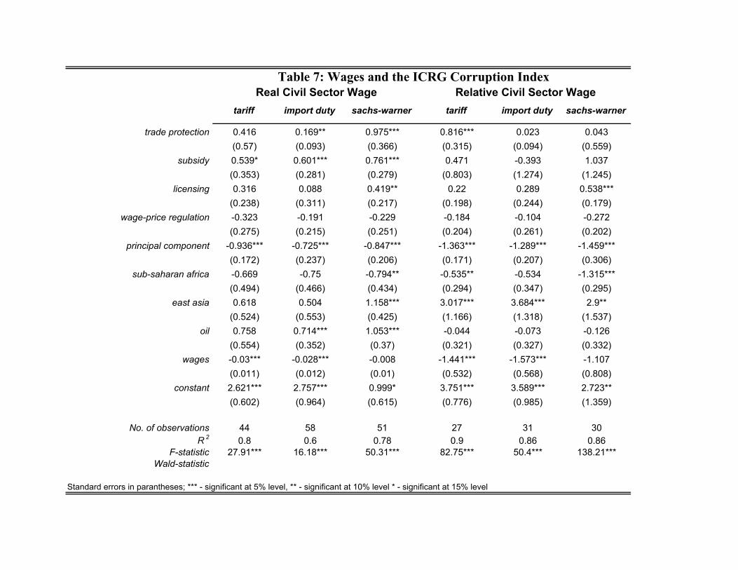
Table 7: Wages and the ICRG Corruption Index

tariff import duty sachs-warner tariff import duty sachs-warner

trade protection 0.416 0.169** 0.975*** 0.816*** 0.023 0.043(0.57) (0.093) (0.366) (0.315) (0.094) (0.559)

subsidy 0.539* 0.601*** 0.761*** 0.471 -0.393 1.037(0.353) (0.281) (0.279) (0.803) (1.274) (1.245)

licensing 0.316 0.088 0.419** 0.22 0.289 0.538***(0.238) (0.311) (0.217) (0.198) (0.244) (0.179)

wage-price regulation -0.323 -0.191 -0.229 -0.184 -0.104 -0.272(0.275) (0.215) (0.251) (0.204) (0.261) (0.202)

principal component -0.936*** -0.725*** -0.847*** -1.363*** -1.289*** -1.459***(0.172) (0.237) (0.206) (0.171) (0.207) (0.306)

sub-saharan africa -0.669 -0.75 -0.794** -0.535** -0.534 -1.315***(0.494) (0.466) (0.434) (0.294) (0.347) (0.295)

east asia 0.618 0.504 1.158*** 3.017*** 3.684*** 2.9**(0.524) (0.553) (0.425) (1.166) (1.318) (1.537)

oil 0.758 0.714*** 1.053*** -0.044 -0.073 -0.126(0.554) (0.352) (0.37) (0.321) (0.327) (0.332)

wages -0.03*** -0.028*** -0.008 -1.441*** -1.573*** -1.107(0.011) (0.012) (0.01) (0.532) (0.568) (0.808)

constant 2.621*** 2.757*** 0.999* 3.751*** 3.589*** 2.723**(0.602) (0.964) (0.615) (0.776) (0.985) (1.359)

No. of observations 44 58 51 27 31 30R 2 0.8 0.6 0.78 0.9 0.86 0.86

F-statistic 27.91*** 16.18*** 50.31*** 82.75*** 50.4*** 138.21***Wald-statistic


Real Civil Sector Wage Relative Civil Sector Wage

Table 8: Instrumental Variables RegressionICRG ICRG ICRG TI TI TI GCOR GCOR GCORtariff import duty sachs-warner tariff import duty sachs-warner tariff import duty sachs-warner

trade protection 6.942* 0.53** 3.215*** 8.273** 0.356* 2.746*** 7.894 0.31* 4.304**(4.477) (0.292) (1.254) (4.598) (0.226) (1.257) (8.516) (0.211) (2.52)

subsidy 0.284*** 0.296 0.396*** 0.908*** 0.95*** 0.966*** 1.475*** 1.966*** 2.486***(0.114) (0.238) (0.185) (0.112) (0.124) (0.121) (0.719) (0.523) (0.865)

licensing 0.501** 0.368 0.364 1.022*** 0.946*** 0.883*** 1.378*** 1.414*** 1.185***(0.251) (0.276) (0.298) (0.351) (0.341) (0.295) (0.499) (0.378) (0.542)

wage-price regulation -0.117 -0.028 0.049 0.498*** 0.269 0.351 0.334 0.98* 1.169*(0.344) (0.268) (0.399) (0.281) (0.297) (0.267) (0.661) (0.592) (0.778)

political rights 0.262*** 0.058 -0.1 0.306*** 0.26** 0.082 0.281 0.431* 0.068(0.113) (0.105) (0.173) (0.153) (0.153) (0.197) (0.264) (0.268) (0.345)

schooling 0.008 0.011 0.009 -0.002 -0.005 0.005 -0.011 -0.02 -0.007(0.011) (0.013) (0.014) (0.014) (0.016) (0.014) (0.029) (0.021) (0.028)

newspapers -0.003*** -0.005*** -0.002 -0.006*** -0.008*** -0.006*** -0.008*** -0.007*** -0.004(0.001) (0.001) (0.002) (0.001) (0.002) (0.001) (0.003) (0.002) (0.004)

sub-saharan africa -0.939 -0.752 -0.652 -1.42*** -1.86*** -1.174*** -2.232 -2.897*** -2.595***(0.932) (0.564) (0.633) (0.448) (0.612) (0.369) (1.569) (1.273) (1.384)

east asia 0.38 0.713 3.178 0.839 1.603*** 3.55*** 3.641*** 3.759*** 7.389***(0.89) (0.766) (0.985) (0.668) (0.668) (0.936) (1.26) (1.054) (2.337)

oil 1.249 1.089** 0.199 3.209*** 2.992*** 2.446***(0.961) (0.542) (0.741) (0.61) (0.574) (0.858)

constant -0.912 0.206 -1.118 -0.643 1.755*** -0.229 -1.1 -2.047 -4.235(1.659) (1.459) (2.169) (1.686) (1.821) (1.691) (3.965) (3.304) (3.998)

No. of observations 49 60 56 44 50 49 34 38 38R 2 0.64 0.4 0.44 0.84 0.76 0.81 0.79 0.77 0.75

F-statistic 15.57*** 7.69*** 18.52*** 102.98*** 43.41*** 161.77*** 24.63*** 50.65*** 41.01***Basmann test 2.823 2.793 0.389 0.24 3.55 0.269 5.3** 3.91 1.402


oes protection beget corruption pushan dutt … · the trade literature has addressed this issue...

Documents