of production engineering, v production engineering of production engineering... · department of...
TRANSCRIPT
Novi Sad, 2010
9 7 7 1 8 2 1 4 9 3 0 0 5
ISSN 1821-4932
Volume 13 No.1
UNIVERSITY OF NOVI SADFaculty of Technical Sciences
Department of Production EngineeringNOVI SAD, SERBIA
UDK 621 ISSN 1821-4932
J O U R N A L O F
PRODUCTION ENGINEERING
JO
UR
NA
L O
F P
RO
DU
CT
IO
N E
NG
IN
EE
RIN
G, V
ol.13, N
o.1, 2010
JO
UR
NA
L O
F P
RO
DU
CT
IO
N E
NG
IN
EE
RIN
G, V
ol.13, N
o.1, 2010
University of Novi Sad FACULTY OF TECHNICAL SCIENCES
DEPARTMENT OF PRODUCTION ENGINEERING 21000 NOVI SAD, Trg Dositeja Obradovica 6, SERBIA
UDK 621 ISSN 1821-4932
JJJOOOUUURRRNNNAAALLL OOOFFF
PPPRRROOODDDUUUCCCTTTIIIOOONNN EEENNNGGGIIINNNEEEEEERRRIIINNNGGG
Volume 13 Number 1
Novi Sad, May 2010

Journal of Production Engineering, Vol.13 (2010), Number 1 Publisher: FACULTY OF TECHNICAL SCIENCES DEPARTMENT OF PRODUCTION ENGINEERING 21000 NOVI SAD, Trg Dositeja Obradovica 6 SERBIA Editor-in-chief: Dr. Pavel Kovač, Professor, Serbia Reviewers: Dr. Miran BREZOČNIK, Professor, Slovenia
Dr. Janko HODOLIČ, Professor, Serbia Dr. Frantisek HOLESOVSKY, Prof., Czech Republic Dr. Vid JOVISEVIC, Professor, Bosnia and Herzegovina Dr. Pavel KOVAČ, Professor, Serbia Dr. Mikolaj KUZINOVSKI, Professor, Macedonia Dr. Ildiko MANKOVA, Professor, Slovak Republic Dr. Jozef NOVAK-MARCINČIN, Prof., Slovak Republic
Dr. Velimir TODIĆ, Professor, Professor, Serbia Dr. Mirko SOKOVIĆ, Assoc. Professor, Slovenia
Dr. Jozef BENO, Assist. Professor, Slovak Republic Dr. Damir GODEC, Assist. Professor, Croatia
Dr. Alan TOPČIĆ, Assist. Professor, Bosnia and Herzeg. Dr. Uroš ZUPERL, Assist. Professor, Slovenia
Technical treatment and design: M.Sc. Miodrag Milošević, Assistant, M.Sc. Borislav Savković, Assistant Manuscript submitted for publication: May 01, 2010. Printing: 1st Circulation: 300 copies CIP classification: Printing by: FTN, Graphic Center GRID, Novi Sad
ISSN: 1821-4932
CIP – Катаголизација у публикацији Библиотека Матице српске, Нови Сад 621 ЈOURNAL of Production Engineering / editor in chief Pavel Kovač. – Vol. 12, No. 1 (2009)- . – Novi Sad : Faculty of Technical Sciences, Department for Production Engineering, 2009-. – 30 cm Godišnje. Je nastavak: Časopis proizvodno mašinstvo = ISSN 0354-6446 ISSN 1821-4932 COBISS.SR-ID 250243079

INTERNATIONAL EDITORIAL BOARD __________________________________________________________________________________ Dr. Joze BALIĆ, Professor, Slovenia Dr. Ljubomir BOROJEV, Professor, Serbia Dr. Konstantin BOUZAKIS, Professor, Greece Dr. Miran BREZOČNIK, Professor, Slovenia Dr. Ilija ĆOSIĆ, Professor, Serbia Dr. Pantelija DAKIĆ, Professor, Bosnia and Herzegovina Dr. Dragan DOMAZET, Professor, Serbia Dr. Katarina GERIĆ, Professor, Serbia Dr. Janko HODOLIČ, Professor, Serbia Dr. František HOLEŠOVSKY, Professor, Czech Republic Dr. Amaia IGARTUA, Professor, Spain Dr. Juliana JAVOROVA, Professor, Bulgaria Dr. Vid JOVIŠEVIĆ, Professor, Bosnia and Herzegovina Dr. Mara KANDEVA, Professor, Professor, Bulgaria Dr. Janez KOPAČ, Professor, Slovenia Dr. Ivan KURIC, Professor, Slovak Republic Dr. Mikolaj KUZINOVSKI, Professor, Macedonia Dr. Miodrag LAZIĆ, Professor, Serbia Dr. Chusak LIMSAKUL, Professor, Thailand Dr. Ljubomir LUKIĆ, Professor, Serbia Dr. Vidosav MAJSTOROVIĆ, Professor, Serbia Dr. Miroslav PLANČAK, Professor, Serbia Dr. Bogdan SOVILJ, Professor, Serbia Dr. Dušan ŠEBO, Professor, Slovak Republic Dr. Peter SUGAR, Professor, , Slovak Republic Dr. Wiktor TARANENKO, Professor, Ukraine Dr. Ljubodrag TANOVIĆ, Professor, Serbia Dr. Velimir TODIĆ, Professor, Serbia Dr. Andrei TUDOR, Professor, Romania Dr. Gyula VARGA, Professor, Hungary Dr. Milan ZELJKOVIĆ, Professor, Serbia Dr. Marin GOSTIMIROVIĆ, Assoc. Professor, Serbia Dr. Miodrag HAĐŽISTEVIĆ, Assoc. Professor, Serbia Dr. Mirko SOKOVIĆ, Assoc. Professor, Slovenia Dr. Branko ŠKORIĆ, Assoc. Professor, Serbia Dr. Milenko SEKULIĆ, Assist. Professor, Serbia Dr. Ognjan LUŽANIN, Assist. Professor, Serbia Dr. Slobodan TABAKOVIĆ, Assist. Professor, Serbia
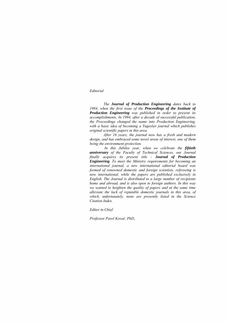
Editorial
The Journal of Production Engineering dates back to 1984, when the first issue of the Proceedings of the Institute of Production Engineering was published in order to present its accomplishments. In 1994, after a decade of successful publication, the Proceedings changed the name into Production Engineering, with a basic idea of becoming a Yugoslav journal which publishes original scientific papers in this area.
After 16 years, the journal now has a fresh and modern design, and has embraced some novel areas of interest, one of them being the environment protection.
In this Jubilee year, when we celebrate the fiftieth anniversary of the Faculty of Technical Sciences, our Journal finally acquires its present title - Journal of Production Engineering. To meet the Ministry requirements for becoming an international journal, a new international editorial board was formed of renowned domestic and foreign scientists, refereeing is now international, while the papers are published exclusively in English. The Journal is distributed to a large number of recipients home and abroad, and is also open to foreign authors. In this way we wanted to heighten the quality of papers and at the same time alleviate the lack of reputable domestic journals in this area, of which, unfortunately, none are presently listed in the Science Citation Index. Editor in Chief Professor Pavel Kovač, PhD,
I
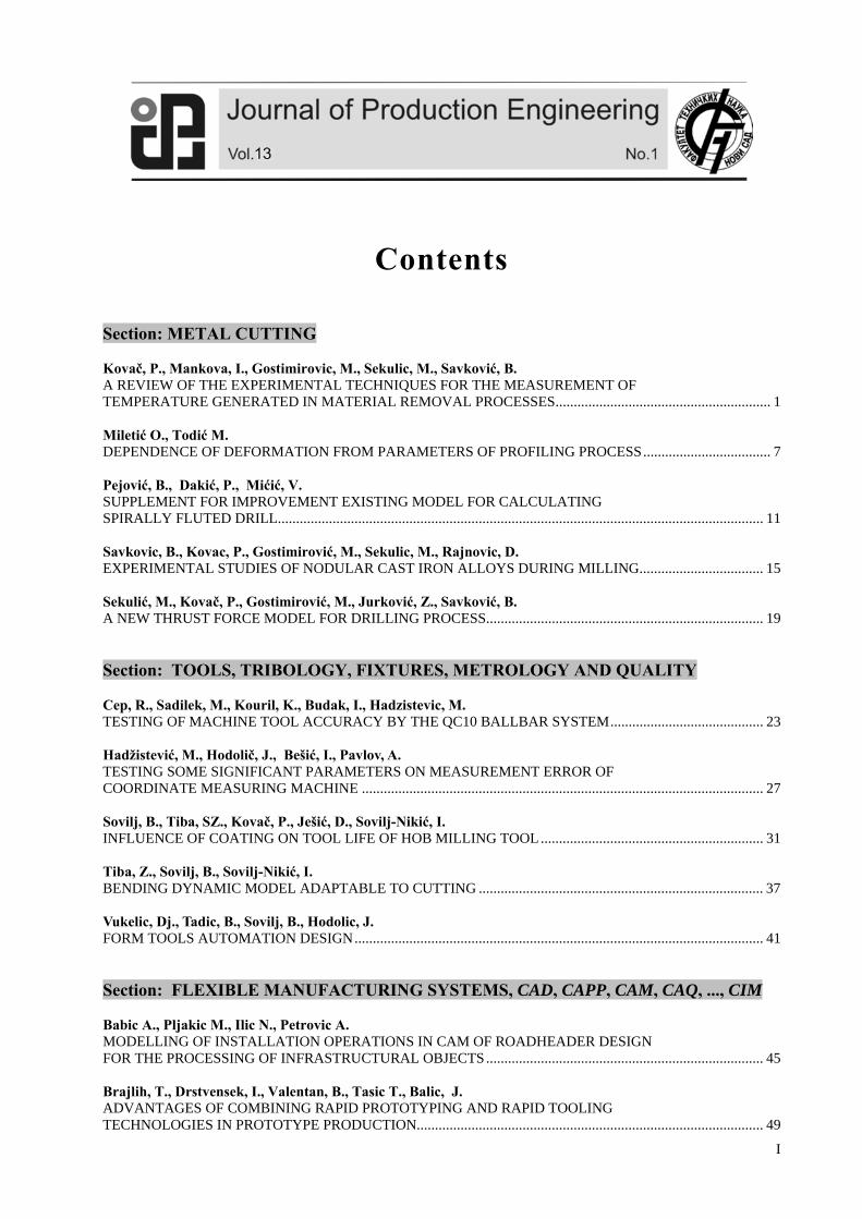
Contents Section: METAL CUTTING Kovač, P., Mankova, I., Gostimirovic, M., Sekulic, M., Savković, B. A REVIEW OF THE EXPERIMENTAL TECHNIQUES FOR THE MEASUREMENT OF TEMPERATURE GENERATED IN MATERIAL REMOVAL PROCESSES........................................................... 1 Miletić O., Todić M. DEPENDENCE OF DEFORMATION FROM PARAMETERS OF PROFILING PROCESS................................... 7 Pejović, B., Dakić, P., Mićić, V. SUPPLEMENT FOR IMPROVEMENT EXISTING MODEL FOR CALCULATING SPIRALLY FLUTED DRILL..................................................................................................................................... 11 Savkovic, B., Kovac, P., Gostimirović, M., Sekulic, M., Rajnovic, D. EXPERIMENTAL STUDIES OF NODULAR CAST IRON ALLOYS DURING MILLING.................................. 15 Sekulić, M., Kovač, P., Gostimirović, M., Jurković, Z., Savković, B. A NEW THRUST FORCE MODEL FOR DRILLING PROCESS............................................................................ 19 Section: TOOLS, TRIBOLOGY, FIXTURES, METROLOGY AND QUALITY Cep, R., Sadilek, M., Kouril, K., Budak, I., Hadzistevic, M. TESTING OF MACHINE TOOL ACCURACY BY THE QC10 BALLBAR SYSTEM.......................................... 23 Hadžistević, M., Hodolič, J., Bešić, I., Pavlov, A.
TESTING SOME SIGNIFICANT PARAMETERS ON MEASUREMENT ERROR OF COORDINATE MEASURING MACHINE .............................................................................................................. 27 Sovilj, B., Tiba, SZ., Kovač, P., Ješić, D., Sovilj-Nikić, I. INFLUENCE OF COATING ON TOOL LIFE OF HOB MILLING TOOL ............................................................. 31 Tiba, Z., Sovilj, B., Sovilj-Nikić, I. BENDING DYNAMIC MODEL ADAPTABLE TO CUTTING .............................................................................. 37 Vukelic, Dj., Tadic, B., Sovilj, B., Hodolic, J. FORM TOOLS AUTOMATION DESIGN................................................................................................................ 41 Section: FLEXIBLE MANUFACTURING SYSTEMS, CAD, CAPP, CAM, CAQ, ..., CIM Babic A., Pljakic M., Ilic N., Petrovic A. MODELLING OF INSTALLATION OPERATIONS IN CAM OF ROADHEADER DESIGN FOR THE PROCESSING OF INFRASTRUCTURAL OBJECTS............................................................................ 45 Brajlih, T., Drstvensek, I., Valentan, B., Tasic T., Balic, J. ADVANTAGES OF COMBINING RAPID PROTOTYPING AND RAPID TOOLING TECHNOLOGIES IN PROTOTYPE PRODUCTION............................................................................................... 49

II
Budak, I., Sokovic, M., Hodolic, J., Kopac, J. POINT DATA REDUCTION BASED ON FUZZY LOGICIN REVERSE ENGINEERING .................................. 53 Luzanin, O., Vilotic, D., Movrin, D. CAM SIMULATION FOR MANUFACTURE OF FORGING DIES FOR CAR WHEEL HUB – A CASE STUDY ........................................................................................................... 57 Matin, I., Hadžistevic, M., Hodolič, J., Vukelić, Dj., Tadić, B. DEVELOPMENT OF CAD/CAE SYSTEM FOR MOLD DESIGN......................................................................... 61 Section: ENVIRONMENTAL TECHNOLOGIES AND ECOLOGICAL SYSTEMS Flimel, M. NEED OF PREDICTIVE ENVIRONMENTAL FRIENDLY SYSTEM OF NOISE PROTECTION............................................................................................................................................................ 65 Hricova, B., Nakatova, H., Badida, M., Lumnitzer, E. APLICATION OF ECODESIGN AND LIFE CYCLE ASSESSMENT IN EVALUATION OF MACHINE PRODUCTS ...................................................................................................... 69 Liptai, P., Badida, M., Lumnitzer, E., Moravec, M. APPLICATION OF ACOUSTIC CAMERA IN INDUSTRIAL SITE ...................................................................... 73 Sebo, J., Fedorcakova, M., Nakatova, H., Sebo, D., Halagovcova, K. OPERATING EXPERIMENT OF WASTEWATER CLEANING AROUND THE BLAST FURNACE IN THE USS-KOSICE ............................................................................................................................ 77 INSTRUCTION FOR CONTRIBUTORS ............................................................................................................. 81
1
Kovač, P., Mankova, I., Gostimirovic, M., Sekulic, M., Savković, B.
A REVIEW OF THE EXPERIMENTAL TECHNIQUES FOR THE MEASUREMENT OF TEMPERATURE GENERATED IN MATERIAL REMOVAL PROCESSES
Abstract: To understand the physical phenomena generated during cutting processes, the characterization of the temperature field is essential. The temperature is an important parameter controlling to tool wear and consequently the life duration, the quality of the surface finish, chip segmentation and the choice of lubrication. Furthermore, thermal aspects become more important with high cutting speeds used presently in industrial processes. A large number of techniques have been developed to quantify the temperature, which can be classified as intrusive (e.g. thermocouple technique) or non-intrusive techniques (e.g. pyrometry technique) Key words: measurement, temperature, material-removing processes 1. INTRODUCTION The most important part of the work generated during the cutting process is converted into heat. There are three main regions concerned with heating during the cutting process: the primary shear zone where the chip is formed is characterized by high shear deformation. The secondary and the tertiary zone where friction and shearing are combined are located respectively along the tool-chip interface and below the tool edge. In these regions, heat is generated and flows into the workpiece, the chip and the tool. Taylor and Komanduri [1] have long appreciated the importance of measuring temperatures during any material removal operation and assessing their effects on both the workpiece and the cutting edge of the tool. While the primary reason for continued work on temperature measurement is to improve the quality of the workpiece surface integrity, it can also help to predict tool wear and aid in the development of predictive software modeling. Furthermore, studies have shown that in material removal processes, phenomena that can degrade workpiece quality can actually be attributed to variations in temperature. In material removal processes, temperature history is directly related to part quality. It can affect dimensional accuracy by causing subsurface damage and introducing residual stresses. On the other hand, if properly controlled, process heat can actually be used to produce desirable workpiece surface hardening. However, in current manufacturing processes
temperature is still not easily measured or controlled. For example, when coolants are used, many current measurement methods do not apply. Since diffusion, chemical reactions and thermal softening depend exponentially on temperature, the productivity and efficiency of material removal operations is adversely affected by increased temperature. Wear of a cutting edge and material diffusion are sensitive to small changes in the local temperatures. Since temperatures at the tool/workpiece interface increase with cutting speed, the associated increase in wear is an important consequence of exponentially activated mechanisms. As an indirect result of accurately measuring temperatures in material removal processes, computer simulations of temperature fields can be improved to include high spatial and temporal resolutions. 2. HISTORICAL PERSPECTIVE The measurement of temperature in material removal processes has an extremely long history, which has been summarized in Figure 1. The number of publications in the field is increasing rapidly and that most methods were first introduced in processes having a single cutting edge with the measurement device affixed to the tool. Some methods such as film thermography have been replaced entirely by solid-state sensors that are more modern, while other methods, such as the dynamic thermocouple, have remained in continuous use for nearly a century.
Fig. 1. Historical outline of thermal measurements in material removal processes [6]
2
Most existing methods for measuring temperature have been applied to material removal processes. The factors that should be considered when choosing a temperature measurement method for a particular application are: (1) temperature range; (2) sensor robustness; (3) temperature field disturbance by the sensor; (4) signal type/sensitivity to noise; (5) response time; and (6) uncertainty. These should be weighed against the following criteria: ease of calibration; availability; cost; and Size.
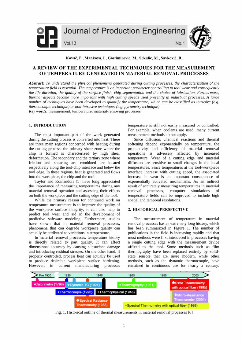
2.1. Calorimetric methods The heat generated in cutting was one of the first and the foremost topics investigated in machining. Pioneering work in this area was due to Benjamin Thompson Count Rumford [2] who in 1798 investigated the heat generated in the boring of cannon and developed the concept of mechanical equivalent of heat. Rumford used the calorimetric method to estimate the heat generated in the boring operation (Figure 2).
Fig. 2 Apparatus for calorimetric measuring of total heat generated in boring [2]
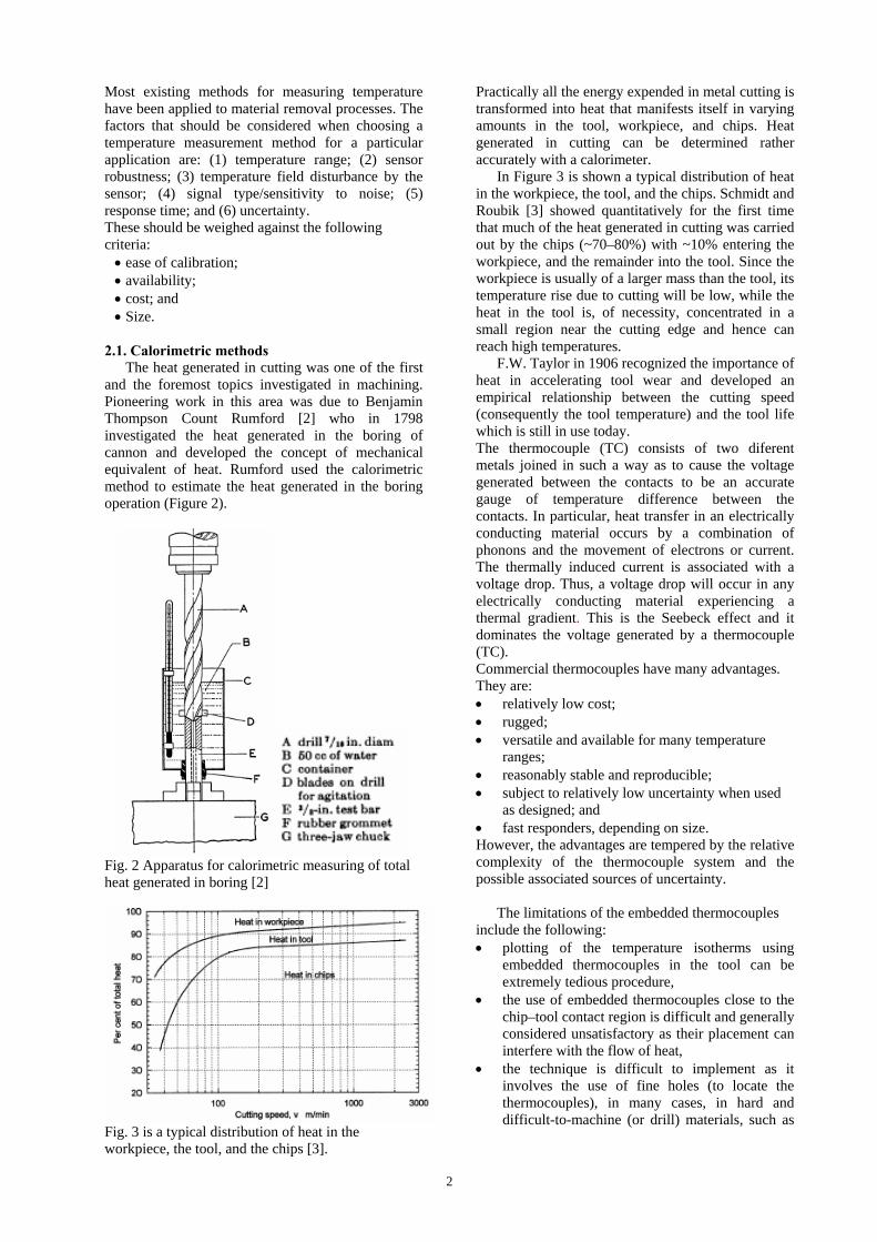
Fig. 3 is a typical distribution of heat in the workpiece, the tool, and the chips [3].
Practically all the energy expended in metal cutting is transformed into heat that manifests itself in varying amounts in the tool, workpiece, and chips. Heat generated in cutting can be determined rather accurately with a calorimeter. In Figure 3 is shown a typical distribution of heat in the workpiece, the tool, and the chips. Schmidt and Roubik [3] showed quantitatively for the first time that much of the heat generated in cutting was carried out by the chips (~70–80%) with ~10% entering the workpiece, and the remainder into the tool. Since the workpiece is usually of a larger mass than the tool, its temperature rise due to cutting will be low, while the heat in the tool is, of necessity, concentrated in a small region near the cutting edge and hence can reach high temperatures. F.W. Taylor in 1906 recognized the importance of heat in accelerating tool wear and developed an empirical relationship between the cutting speed (consequently the tool temperature) and the tool life which is still in use today. The thermocouple (TC) consists of two diferent metals joined in such a way as to cause the voltage generated between the contacts to be an accurate gauge of temperature difference between the contacts. In particular, heat transfer in an electrically conducting material occurs by a combination of phonons and the movement of electrons or current. The thermally induced current is associated with a voltage drop. Thus, a voltage drop will occur in any electrically conducting material experiencing a thermal gradient. This is the Seebeck effect and it dominates the voltage generated by a thermocouple (TC). Commercial thermocouples have many advantages. They are: relatively low cost; rugged; versatile and available for many temperature
ranges; reasonably stable and reproducible; subject to relatively low uncertainty when used
as designed; and fast responders, depending on size. However, the advantages are tempered by the relative complexity of the thermocouple system and the possible associated sources of uncertainty. The limitations of the embedded thermocouples include the following: plotting of the temperature isotherms using
embedded thermocouples in the tool can be extremely tedious procedure,
the use of embedded thermocouples close to the chip–tool contact region is difficult and generally considered unsatisfactory as their placement can interfere with the flow of heat,
the technique is difficult to implement as it involves the use of fine holes (to locate the thermocouples), in many cases, in hard and difficult-to-machine (or drill) materials, such as
3
ceramics, cemented carbides, and hardened HSS tools,
the temperature gradients at the surface are rather steep and in many situations have to be estimated as it would be difficult to locate two thermocouples very close to each other, and
thermocouples have limited transient response due to their mass and distance from the points of intimate contact.
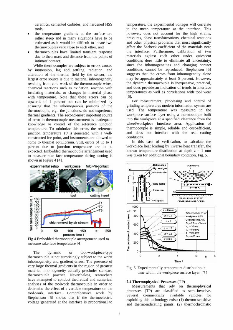
While thermocouples are subject to errors caused by immersion, lag and settling, radiation, and alteration of the thermal field by the sensor, the largest error source is due to material inhomogeneity resulting from cold work of the thermocouple wires, chemical reactions such as oxidation, reaction with insulating materials, or changes in material phase with temperature. Note that these errors can be upwards of 1 percent but can be minimized by ensuring that the inhomogenous portions of the thermocouple, e.g., the junctions, do not experience thermal gradients. The second-most important source of error in thermocouple measurement is inadequate knowledge or control of the reference junction temperature. To minimize this error, the reference junction temperature T0 is generated with a well-constructed ice point, and instruments are allowed to come to thermal equilibrium. Still, errors of up to 1 percent due to junction temperature are to be expected. Embedded thermocouple arrangement used to measure rake face temperature during turning is shown in Figure 4 [4].
Fig 4 Embedded thermocouple arrangement used to measure rake face temperature [4] The dynamic or tool-workpiece-type thermocouple is not surprisingly subject to the worst inhomogeneity and gradient errors. The presence of very large thermal gradients in the region of greatest material inhomogeneity actually precludes standard thermocouple practice. Nevertheless, researchers have attempted to conduct theoretical and numerical analyses of the toolwork thermocouple in order to determine the effect of a variable temperature on the tool-work interface. Comprehensive work by Stephenson [5] shows that if the thermoelectric voltage generated at the interface is proportional to
temperature, the experimental voltages will correlate to the mean temperature at the interface. This however, does not account for the high strains, pressures, phase transformations, chemical reactions and other physical problems that must significantly affect the Seebeck coefficient of the materials near the interface. Furthermore, calibration of two materials against each other under quiescent conditions does little to eliminate all uncertainty, since the inhomogeneities and changing contact conditions cannot be reproduced. Stephenson [5] suggests that the errors from inhomogeneity alone may be approximately at least 5 percent. However, the dynamic thermocouple is inexpensive, practical, and does provide an indication of trends in interface temperatures as well as correlations with tool wear [6].
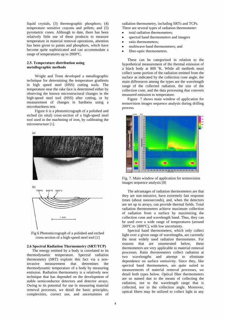
For measurement, processing and control of grinding temperatures modern information system are used. The temperature was measured in the workpiece surface layer using a thermocouple built into the workpiece at a specified clearance from the wheel/workpiece interface area. Application of thermocouple is simple, reliable and cost-efficient, and does not interfere with the real cutting conditions.
In this case of verification, to calculate the workpiece heat loading by inverse heat transfer, the known temperature distribution at depth z = 1 mm was taken for additional boundary condition, Fig. 5.
Fig. 5 Experimentally temperature distribution in time within the workpiece surface layer [7]
2.4 Thermophysical Processes (TP) Measurements that rely on thermophysical processes (TP) are classified as semi-invasive. Several commercially available vehicles for exploiting this technology exist: (1) thermo-sensitive and thermoindicating paints, (2) thermochromatic
4
liquid crystals, (3) thermographic phosphors; (4) temperature sensitive crayons and pellets; and (5) pyrometric cones. Although to date, there has been relatively little use of these products to measure temperature in material removal operations, attention has been given to paints and phosphors, which have become quite sophisticated and can accommodate a range of temperatures up to 2000ºC. 2.5. Temperature distribution using metallographic methods
Wright and Trent developed a metallographic technique for determining the temperature gradients in high speed steel (HSS) cutting tools. The temperature near the rake face is determined either by observing the known microstructural changes in the high-speed steel tool (HSS) after cutting, or by measurement of changes in hardness using a microhardness test.
Figure 6 is a photomicrograph of a polished and etched (in nital) cross-section of a high-speed steel tool used in the machining of iron, by calibrating the microstructure [1].
Fig 6 Photomicrograph of a polished and etched
cross-section of a high-speed steel tool [1] 2.6 Spectral Radiation Thermometry (SRT/TCP) The energy emitted by a body is correlated to its thermodynamic temperature. Spectral radiation thermometry (SRT) exploits this fact via a non-invasive measurement that determines the thermodynamic temperature of a body by measuring emission. Radiation thermometry is a relatively new technique that has depended on the development of stable semiconductor detectors and detector arrays. Owing to its potential for use in measuring material removal processes, we detail the basic principles, complexities, correct use, and uncertainties of
radiation thermometry, including SRTs and TCPs. There are several types of radiation thermometer: total radiation thermometers; spectral band thermometers and imagers ratio thermometers; multiwave band thermometers; and fiber-optic thermometers. These can be categorized in relation to the hypothetical measurement of the thermal emission of a black body at 800 ºK. While all methods must collect some portion of the radiation emitted from the surface as indicated by the collection cone angle, the main differences among the types are the wavelength range of the collected radiation, the size of the collection cone, and the data processing that converts measured emission to temperature. Figure 7 shows main window of application for termovision images sequence analysis during drilling process.
Fig. 7. Main window of application for termovision images sequence analysis [8] The advantages of radiation thermometers are that they are non-intrusive, have extremely fast response times (about nanoseconds), and, when the detectors are set up in arrays, can provide thermal fields. Total radiation thermometers achieve maximum collection of radiation from a surface by maximizing the collection cone and wavelength band. Thus, they can be used over a wide range of temperatures (around 200ºC to 1800ºC), with low uncertainty. Spectral band thermometers, which only collect light over a given range of wavelengths, are currently the most widely used radiation thermometer. For reasons that are enumerated below, these thermometers are very applicable to material removal processes. Ratio thermometers collect radiation at two wavelengths and attempt to eliminate dependence on surface emissivity. Since they, like spectral band thermometers, are quite suited to measurements of material removal processes, we detail both types below. Optical fiber thermometers are so named due to the means of collecting the radiation, not to the wavelength range that is collected, nor to the collection angle. Moreover, optical fibers may be utilized to collect light in any
5
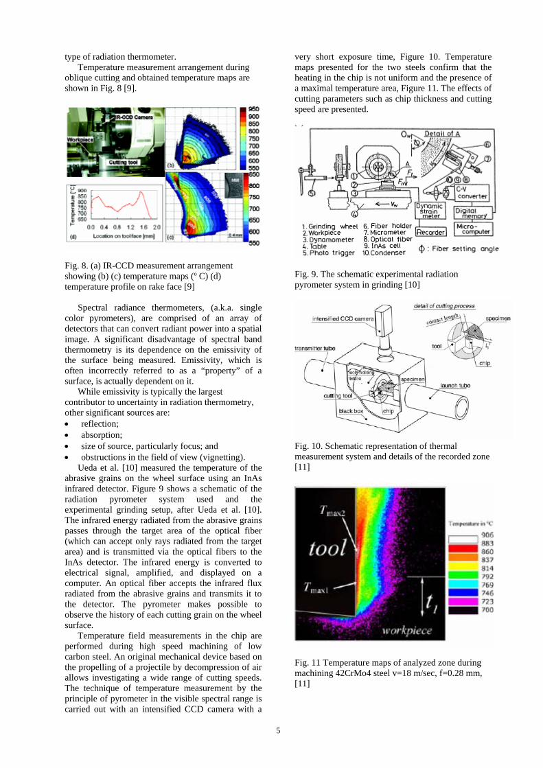
type of radiation thermometer. Temperature measurement arrangement during oblique cutting and obtained temperature maps are shown in Fig. 8 [9].
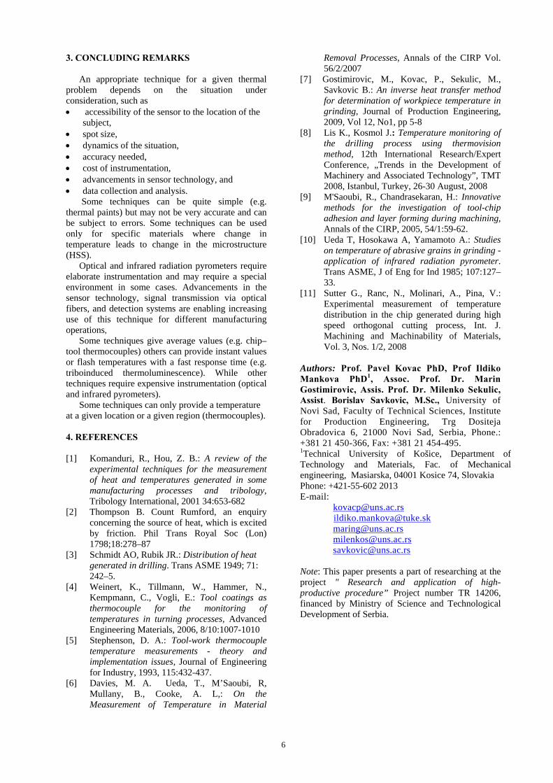
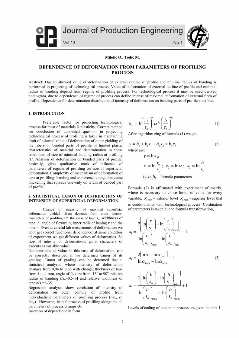
Fig. 8. (a) IR-CCD measurement arrangement showing (b) (c) temperature maps (º C) (d) temperature profile on rake face [9] Spectral radiance thermometers, (a.k.a. single color pyrometers), are comprised of an array of detectors that can convert radiant power into a spatial image. A significant disadvantage of spectral band thermometry is its dependence on the emissivity of the surface being measured. Emissivity, which is often incorrectly referred to as a “property” of a surface, is actually dependent on it. While emissivity is typically the largest contributor to uncertainty in radiation thermometry, other significant sources are: reflection; absorption; size of source, particularly focus; and obstructions in the field of view (vignetting). Ueda et al. [10] measured the temperature of the abrasive grains on the wheel surface using an InAs infrared detector. Figure 9 shows a schematic of the radiation pyrometer system used and the experimental grinding setup, after Ueda et al. [10]. The infrared energy radiated from the abrasive grains passes through the target area of the optical fiber (which can accept only rays radiated from the target area) and is transmitted via the optical fibers to the InAs detector. The infrared energy is converted to electrical signal, amplified, and displayed on a computer. An optical fiber accepts the infrared flux radiated from the abrasive grains and transmits it to the detector. The pyrometer makes possible to observe the history of each cutting grain on the wheel surface. Temperature field measurements in the chip are performed during high speed machining of low carbon steel. An original mechanical device based on the propelling of a projectile by decompression of air allows investigating a wide range of cutting speeds. The technique of temperature measurement by the principle of pyrometer in the visible spectral range is carried out with an intensified CCD camera with a
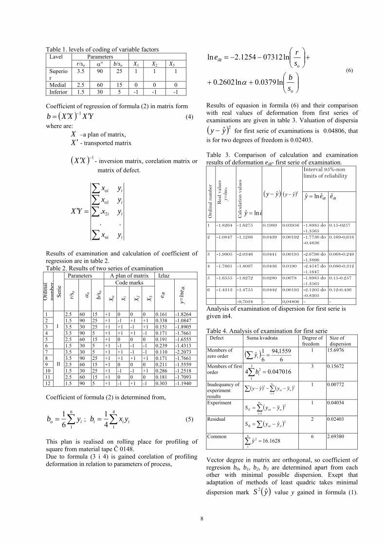
very short exposure time, Figure 10. Temperature maps presented for the two steels confirm that the heating in the chip is not uniform and the presence of a maximal temperature area, Figure 11. The effects of cutting parameters such as chip thickness and cutting speed are presented.
Fig. 9. The schematic experimental radiation pyrometer system in grinding [10]
Fig. 10. Schematic representation of thermal measurement system and details of the recorded zone [11]
Fig. 11 Temperature maps of analyzed zone during machining 42CrMo4 steel v=18 m/sec, f=0.28 mm, [11]
6
3. CONCLUDING REMARKS
An appropriate technique for a given thermal problem depends on the situation under consideration, such as accessibility of the sensor to the location of the
subject, spot size, dynamics of the situation, accuracy needed, cost of instrumentation, advancements in sensor technology, and data collection and analysis.
Some techniques can be quite simple (e.g. thermal paints) but may not be very accurate and can be subject to errors. Some techniques can be used only for specific materials where change in temperature leads to change in the microstructure (HSS).
Optical and infrared radiation pyrometers require elaborate instrumentation and may require a special environment in some cases. Advancements in the sensor technology, signal transmission via optical fibers, and detection systems are enabling increasing use of this technique for different manufacturing operations,
Some techniques give average values (e.g. chip–tool thermocouples) others can provide instant values or flash temperatures with a fast response time (e.g. triboinduced thermoluminescence). While other techniques require expensive instrumentation (optical and infrared pyrometers).
Some techniques can only provide a temperature at a given location or a given region (thermocouples). 4. REFERENCES [1] Komanduri, R., Hou, Z. B.: A review of the
experimental techniques for the measurement of heat and temperatures generated in some manufacturing processes and tribology, Tribology International, 2001 34:653-682
[2] Thompson B. Count Rumford, an enquiry concerning the source of heat, which is excited by friction. Phil Trans Royal Soc (Lon) 1798;18:278–87
[3] Schmidt AO, Rubik JR.: Distribution of heat generated in drilling. Trans ASME 1949; 71: 242–5.
[4] Weinert, K., Tillmann, W., Hammer, N., Kempmann, C., Vogli, E.: Tool coatings as thermocouple for the monitoring of temperatures in turning processes, Advanced Engineering Materials, 2006, 8/10:1007-1010
[5] Stephenson, D. A.: Tool-work thermocouple temperature measurements - theory and implementation issues, Journal of Engineering for Industry, 1993, 115:432-437.
[6] Davies, M. A. Ueda, T., M’Saoubi, R, Mullany, B., Cooke, A. L,: On the Measurement of Temperature in Material
Removal Processes, Annals of the CIRP Vol. 56/2/2007
[7] Gostimirovic, M., Kovac, P., Sekulic, M., Savkovic B.: An inverse heat transfer method for determination of workpiece temperature in grinding, Journal of Production Engineering, 2009, Vol 12, No1, pp 5-8
[8] Lis K., Kosmol J.: Temperature monitoring of the drilling process using thermovision method, 12th International Research/Expert Conference, „Trends in the Development of Machinery and Associated Technology”, TMT 2008, Istanbul, Turkey, 26-30 August, 2008
[9] M'Saoubi, R., Chandrasekaran, H.: Innovative methods for the investigation of tool-chip adhesion and layer forming during machining, Annals of the CIRP, 2005, 54/1:59-62.
[10] Ueda T, Hosokawa A, Yamamoto A.: Studies on temperature of abrasive grains in grinding - application of infrared radiation pyrometer. Trans ASME, J of Eng for Ind 1985; 107:127–33.
[11] Sutter G., Ranc, N., Molinari, A., Pina, V.: Experimental measurement of temperature distribution in the chip generated during high speed orthogonal cutting process, Int. J. Machining and Machinability of Materials, Vol. 3, Nos. 1/2, 2008
Authors: Prof. Pavel Kovac PhD, Prof Ildiko Mankova PhD1, Assoc. Prof. Dr. Marin Gostimirovic, Assis. Prof. Dr. Milenko Sekulic, Assist. Borislav Savkovic, M.Sc., University of Novi Sad, Faculty of Technical Sciences, Institute for Production Engineering, Trg Dositeja Obradovica 6, 21000 Novi Sad, Serbia, Phone.: +381 21 450-366, Fax: +381 21 454-495. 1Technical University of Košice, Department of Technology and Materials, Fac. of Mechanical engineering, Masiarska, 04001 Kosice 74, Slovakia Phone: +421-55-602 2013 E-mail: [email protected]
[email protected] [email protected] [email protected] [email protected] Note: This paper presents a part of researching at the project " Research and application of high-productive procedure” Project number TR 14206, financed by Ministry of Science and Technological Development of Serbia.
7
Miletić O., Todić M.
DEPENDENCE OF DEFORMATION FROM PARAMETERS OF PROFILING PROCESS
Abstract: Due to allowed value of deformation of external outline of profile and minimal radius of banding is performed in projecting of technological process. Value of deformation of external outline of profile and minimal radius of banding depend from regime of profiling process. For technological process it may be used derived nomogram, due to dependence of regime of process can define intense of maximal deformation of external fibro of profile. Dependence for determination distribution of intensity of deformation on banding parts of profile is defined. 1. INTRODUCTION Preferable factor for projecting technological process for most of materials is plasticity. Correct method for conclusion of appointed question in projecting technological process of profiling is taken in maintaining limit of allowed value of deformation of outer yielding of the fibers on bended parts of profile of limited plastic characteristics of material and determination in these conditions of size of minimal banding radius at profiling /1/. Analysis of deformation on bended parts of profile, basically, gives qualitative mark of influence of parameters of regime of profiling on size of superficial deformation. Complexity of mechanism of deformation of tape at profiling: banding and transversal elongation cause thickening that spreads unevenly on width of bended part of profile. 2. STATISTICAL CANON OF DISTRIBUTION OF INTENSITY OF SUPERFICIAL DEFORMATION Change of intensity of maximal superficial deformation yielded fibers depends from more factors-parameters of profiling /2/: thickness of tape so, widthness of tape b, angle of flexure , inner radis of baning r and the others. Even at careful lab mesurments of deformation we dont get correct functional dependence: at same conditios of experiment we get different values of deformatios. So size of intesity of deformations gains characters of axdents as variable value. Nondeterminated value, in this case of deformation, can be correctly described if we determed canon of its grading. Canon of grading can be determed due ti statistical analysis; where intensity of deformation changes from 0,04 to 0,66 with change; thickness of tape from 1 to 4 mm, angle of flexure from 15o to 90o, relative radius of banding r/so=0,5-14 and relative widthness of tape b/so=6-35. Regression analysis show corelation of intensity of deformation on outer conture of profile from individualistic parameters of profiling process (r/so, , b/so). However, in real process of profiling alongtime all parameters of process change /3/. Insertion of dependence in form,
3
2
1
/b
o
b
b
oik s
b
s
rBe
(1)
After logarithm zing of formula (1) we get,
332211 xbxbxbby o (2)
where are:
ikey ln
o
o
s
rx ln1 ; ln2 x ;
os
bx ln3
3,21, bbb - formula parameters
Formula (2) is affirmated with experiment of matrix, where is necessary to chose limits of value for every
variable, minix – inferior level maxix - superior level that
is conditionality with technological process. Cordination of parameters is taken due to formula transformation,
1
lnln
lnln2
minmax
max1
oo
oo
s
r
s
r
s
r
s
r
x
1lnln
lnln2
minmax
max1
x (3)
1
lnln
lnln2
minmax
max3
oo
oo
s
b
s
b
s
b
s
b
x
Levels of coding of factors in process are given in table 1.
8
Table 1. levels of coding of variable factors Parameters Lavel
r/so o b/so X1 X2 X3 Superior
3.5 90 25 1 1 1
Medial 2.5 60 15 0 0 0 Inferior 1.5 30 5 -1 -1 -1
Coefficient of regression of formula (2) in matrix form
YXXXb 1 (4)
where are: X –a plan of matrix, X - transported matrix
1XX - inversion matrix, corelation matrix or
matrix of defect.
ini
ii
io
ioi
yx
yx
yx
yx
YX
..
. 2
1
Results of examination and calculation of coefficient of regression are in table 2. Table 2. Results of two series of examination
Paraneters A plan of matrix Izlaz Code marks
Ord
inal
nu
mbe
rS
erie
r/s o
o
b/s o
Xo
X1
X2
X3 e i
R
y=ln
e iR
1 2.5 60 15 +1 0 0 0 0.161 -1.8264 2 1.5 90 25 +1 -1 +1 +1 0.338 -1.0847 3 3.5 30 25 +1 +1 -1 +1 0.151 -1.8905 4 3.5 90 5 +1 +1 +1 -1 0.171 -1.7661 5 2.5 60 15 +1 0 0 0 0.191 -1.6555 6
I
1.5 30 5 +1 -1 -1 -1 0.239 -1.4313 7 3.5 30 5 +1 +1 -1 -1 0.110 -2.2073 8 3.5 90 25 +1 +1 +1 +1 0.171 -1.7661 9 2.5 60 15 +1 0 0 0 0.211 -1.5559 10 1.5 30 25 +1 -1 -1 +1 0.286 -1.2518 11 2.5 60 15 +1 0 0 0 0.181 -1.7093 12
II
1.5 90 5 +1 -1 +1 -1 0.303 -1.1940 Coefficient of formula (2) is determined from,
6
16
1io yb ;
4
14
1iii yxb (5)
This plan is realised on rolling place for profiling of square from material tape Č 0148. Due to formula (3 i 4) is gained corelation of profiling deformation in relation to parameters of process,
o
oiR
s
b
s
re
ln0379.0ln2602.0
ln073121254.2ln
(6)
Results of equasion in formila (6) and their comparison with real values of deformation from first series of examinations are given in table 3. Valuation of dispersia
2yy for first serie of examinations is 0.04806, that
is for two degrees of freedom is 0.02403. Table 3. Comparison of calculation and examination results of deformation eiR- first serie of examination.
Interval 95%-non limits of reliability
Ord
inal
num
ber
Rea
l val
ues
y=ln
eiR
Cal
cula
tion
val
ues
ey ˆlnˆ
yy ˆ
2yy
iRey ˆlnˆ iRe
1 -1.8264 -1.6275 0.1989 0.03956 -1.8985 do -1.3565
0.15-0257
2 -1.0847 -1.1286 0.0439 0.00192 -1.7736 do -0.4836
0.169-0,616
3 -1.9905 -2.0346 0.0441 0.00195 -2.6796 do -1.3896
0.068-0.249
4 -1.7661 -1.8097 0.0436 0.0190 -2.4547 do -1.1647
0.086-0.312
5 -1.6555 -1.6272 0.0280 0.0078 -1.8985 do -1.3565
0.15-0.257
6 -1.4313 -1.4755 0.0442 0.00195 -2.1205 do -0.8305
0.12-0.436
-9,7034 - 0,04806 - -
Analysis of examination of dispersion for first serie is given in4. Table 4. Analysis of examination for first serie
Defect Suma kvadrata Degree of freedom
Size of dispersion
Members of zero order
6
1559,94
6
1ˆ iy
1 15.6976
Members of first order
3
1
2 047016.04 ib 3 0.15672
Inadequancy of experiment results
on
iooi yyyy
1
22ˆ 1 0.00772
Experiment
on
iooiE yyS
1
2 1 0.04034
Residual 2ˆooiR yyS 2 0.02403
Common
6
1
2 1628.16y 6 2.69380
Vector degree in matrix are orthogonal, so coefficient of regresion b0, b1, b2, b3 are determined apart from each other with minimal possible dispersion. Exept that adaptation of methods of least quadric takes minimal
dispersion mark yS ˆ2 value y gained in formula (1).
9
Method has importance because it rely on empirical values y that are not connected, it is considered that defect of experiment of normal grading and has equally dispersion. Limit of defects for logharitm intensity of deformation is gained from relation
ySty f ˆˆ 2, (5a)
From relation (5a) interval of reliability for logharitm of deformation,
1ˆˆˆlnˆˆ 2,
2, yStyeyStyP fiRf
where are: y - calculation values lneiR, formula (5)
,ft - grading of Students, at f degree of freedom(1-)
level of probability
yS ˆ2 - mark of dispersion y , determined due to matrix
1XX and rest of the dispersion.
Evaluation of the rest of dispersion S2 is based on summ of quadrats of different values of logharitm deformation. For first examination serie of summ of quadrats lneiR deviation is 0.04806 (table 3). For two deegres of freedom markof the rest of dispersion S2=0,02403. Mark of
dispersion iReyS lnˆ2 is taken in analogy with
conditions of examination, so for examinations 2,3,4,6
based on matrix 1XX ,
222
12
11
4
1
4
1
4
1
6
1ˆ SSyS
and for examinations 1 i 5
22
6
1ˆ SyS .
Interval of credibility for examinations 2, 3, 4, 6 at 95%-om interval of confidenc and two deegres of freedom (at t2;0.05),
645,0ˆ15,03,4ˆ12
11ˆ 2
05.0;2 yySty
and for examinations 1 i 5
271,0ˆ63,03,4ˆ6
1ˆ 2
05.0;2 yySty
For evaluation of results of first serie of examinations is necessary to determine and to analyse mark of dispersion and to check adequacy of hypothesis of matematical model. For analysis is determined: 1. Basic summ of quadrats 2y consists of summ of
quadrats of the rest 2yy and summ of quadrats of
regression 22 yyy
2.Summ of quadrats of regression consists from summ of qudrats conditionaled by model of zero order and summ of quadrats conditionaled by model of first 3.Summ of quadrats consists from summ of quadrats and relative defect of experiment, and summ of quadrats that makes inadequacy of presenting results of experiments
on
ooi yyyy1
22ˆ
Analysis of dispersion mark for first serie of experiments is given in table 4. Comparation of dispersion marks, relative inadequancy of presenting results of experiments, with dispersion mark of experiment defect, is given with Fishers F-grading. For first serie of examination F=0,19; for P=0,95 and f1=f2=1 FT=164,4, points that gained matematical model (5) is adequat. Calculated interval of credibility (table 3) show that is necessary to confirm results of experiments by reapting of experiment, what is obvious, that intervals are wide and does not enable use of gained formula. So, it is necessary to do second serie of experiments (6-12) whose results are given in table 2. Due to this datas next formula is presented
ooiR s
b
s
re ln1189.0ln2269.0ln9005.00344.2ln (6)
Statistic alanalysis of results of second serie of examination is taken analogisally to analysis of firs serie of examination. N requards to all differences beetwen two series, gasined formulas are similar, which makes possible to unite results of first and second serie. Coeficient of united series of examinations can be determed as average value of formula (5) and (6):
ooiR s
b
s
re ln780.0ln2435.0ln8158.00799.2ln (7)
Interval of credibility are: 1570.0ˆ y - for examinations 2-4, 6-8, 10, 12 i
0693.0ˆ y - for examinations 1, 5, 9, 11.
Common adequacy of model (7), is taken by analysis of dispersion mark (table 5). Table 5. Analysis of dispersion mark of unated series of examination Defect Summ of quadrats Deegre
of freedom
Size of dispersion
Members of zero order
12
9533,372
12
1212
1
iy 1 31,080
Members of first order
3
1
2 5664.04 ib 3 0.1888
Inadequacy of results of experiments
024887.0ˆ1
22
on
iooi yyyy
5 0.004977
Experiments 056971,01
2
on
iooiE yyS
1 0.01899
Residual 081858.0ˆ 2 yySR
8 0.010232
Common 12
1
2 3572.32y 12 2.6964
3. CONCLUSION Formula (7) can be transformated in natural form by transformation from logharitm to numerical parameters
10
816.0
078.0
244.0125.0
o
oiR
s
r
s
b
e
(8)
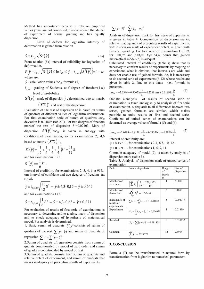
Due to formula (8) is gained nomogram (picture 1) according to dependence from regime of profiling can be determed intensity of maximal logharitm deformation of outer fibers of profile, and intensity of deformation on inner area of profile eiR and maximal stress in profile.
10
0.1
0.15
0.20
0.25
0.30
e iR
0.35
0.40
0.45
0.50
20
30
40
b/s=
5o r/s =1o
r/s =1,5o
r/s =2o
r/s =2,5o
r/s =3,5o
r/s =3,5o
b/s =10o
b/s =15o
b/s =20o
b/s =25o
b/s =30o
50
60
70
80
90
Slika 1. Nomogram for determination of maximal superficial deformation in relation to parameters of profiling Intensity of maximal deformation of profile in evert shaped cell, and what is necessary at projecting regime of profiling, based on plastic characteristics of material, is determined from differences of intensity of deformation of profile beetwen last and previous cell. Due to these differences and formula (8) can be determed and minimal allowed radius of banding by profiling ( results of examination of materials by extension).
e iR
0.10
0.20r=3, 0-90o
r= .5, 0-906o20
20
=2,5
r
e iR
0.10
0.20
40
30
=3
45or=4
e iR
0.10
0.20
40
30
=3
60or=4
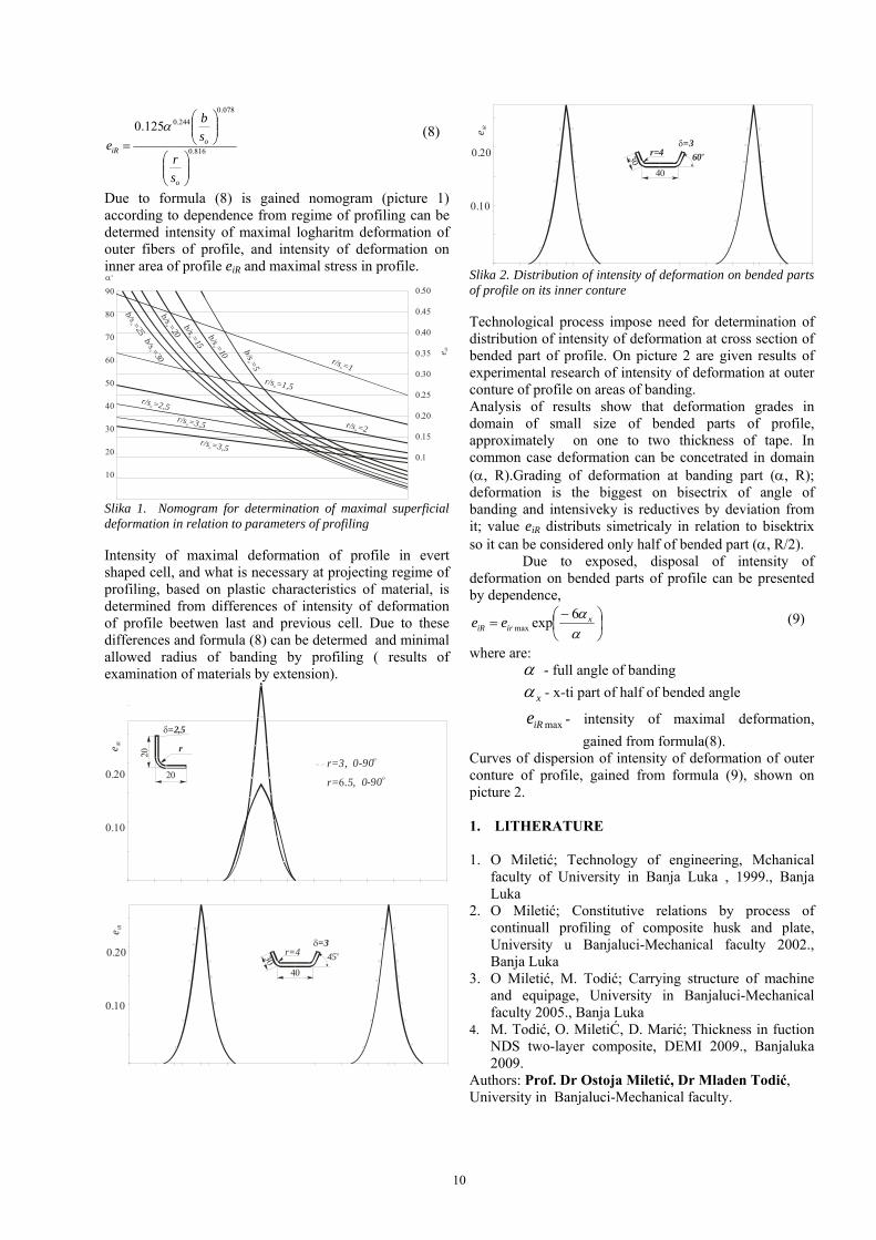
Slika 2. Distribution of intensity of deformation on bended parts of profile on its inner conture Technological process impose need for determination of distribution of intensity of deformation at cross section of bended part of profile. On picture 2 are given results of experimental research of intensity of deformation at outer conture of profile on areas of banding. Analysis of results show that deformation grades in domain of small size of bended parts of profile, approximately on one to two thickness of tape. In common case deformation can be concetrated in domain (, R).Grading of deformation at banding part (, R); deformation is the biggest on bisectrix of angle of banding and intensiveky is reductives by deviation from it; value eiR distributs simetricaly in relation to bisektrix so it can be considered only half of bended part (, R/2). Due to exposed, disposal of intensity of deformation on bended parts of profile can be presented by dependence,
x
iriR ee6
expmax (9)
where are: - full angle of banding
x - x-ti part of half of bended angle
maxiRe - intensity of maximal deformation,
gained from formula(8). Curves of dispersion of intensity of deformation of outer conture of profile, gained from formula (9), shown on picture 2. 1. LITHERATURE 1. O Miletić; Technology of engineering, Mchanical
faculty of University in Banja Luka , 1999., Banja Luka
2. O Miletić; Constitutive relations by process of continuall profiling of composite husk and plate, University u Banjaluci-Mechanical faculty 2002., Banja Luka
3. O Miletić, M. Todić; Carrying structure of machine and equipage, University in Banjaluci-Mechanical faculty 2005., Banja Luka
4. M. Todić, O. MiletiĆ, D. Marić; Thickness in fuction NDS two-layer composite, DEMI 2009., Banjaluka 2009.
Authors: Prof. Dr Ostoja Miletić, Dr Mladen Todić, University in Banjaluci-Mechanical faculty.
11
Pejović, B., Dakić, P., Mićić, V.
SUPPLEMENT FOR IMPROVEMENT EXISTING MODEL FOR CALCULATING SPIRALLY FLUTED DRILL
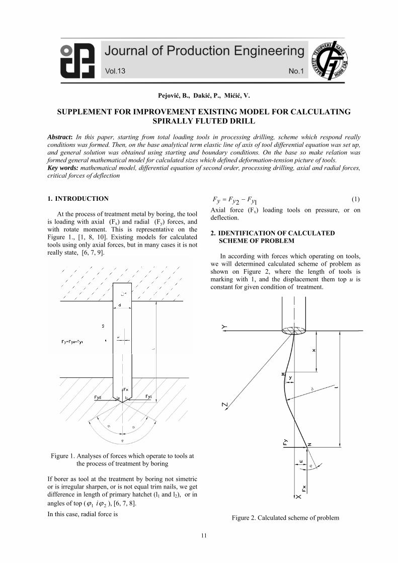
Abstract: In this paper, starting from total loading tools in processing drilling, scheme which respond really conditions was formed. Then, on the base analytical term elastic line of axis of tool differential equation was set up, and general solution was obtained using starting and boundary conditions. On the base so make relation was formed general mathematical model for calculated sizes which defined deformation-tension picture of tools. Key words: mathematical model, differential equation of second order, processing drilling, axial and radial forces, critical forces of deflection 1. INTRODUCTION At the process of treatment metal by boring, the tool is loading with axial (Fx) and radial (Fy) forces, and with rotate moment. This is representative on the Figure 1., [1, 8, 10]. Existing models for calculated tools using only axial forces, but in many cases it is not really state, [6, 7, 9].
Figure 1. Analyses of forces which operate to tools at
the process of treatment by boring If borer as tool at the treatment by boring not simetric or is irregular sharpen, or is not equal trim nails, we get difference in length of primary hatchet (l1 and l2), or in angles of top ( 21 i ), [6, 7, 8].
In this case, radial force is
12 yFyFyF (1)
Axial force (Fx) loading tools on pressure, or on deflection. 2. IDENTIFICATION OF CALCULATED SCHEME OF PROBLEM In according with forces which operating on tools, we will determined calculated scheme of problem as shown on Figure 2, where the length of tools is marking with 1, and the displacement them top u is constant for given condition of treatment.
Figure 2. Calculated scheme of problem
12
3. Differential equation of problem Equation of elastic line of axis tool, because work forces Fx and Fy, in general case we can show as y=f(x) Curve for every point M(x,y) of elastic line will be, [4, 5, 11],
32 )'1(
''1
y
y
(2)
According elastic theory, curve of neutral line can be shown in form , [3, 11],
EI
M
1
(3)
In relation (3), M is moment twist and EI is inflexibility joist at same tension. When equation (2) is equal equation (3), we get,
EI
M
y
y
32 )'1(
'' (4)
Curves of tangente are little variables, 2'y is little
variable, because 2'y ‹‹ l, term (4) transform in ,
[2, 11],
EI
My '' (5)
Term (5) is analytical term of elastic line, where sign depends of orientation coordinate axis. For our case, Fig. 2, elastic line is convex in the direction of positive y- axis, and for every point ''y <0, [4, 5].
In term (5), EI
M is a positive variable. Under activity
forces Fx, Fy stick is twisting and have curve y on the distance x. In this section moment is, M=Fx(u+y)+Fy(l-x) (6) Replacing moment from equation (6) in relation (5), we get,
EI
xlFyuFy
yx )()(''
(7)
and,
)()('' xlEI
Fyu
EI
Fy
yx (8)
Now we introduce parametar k2,
2kEI
Fx (9)
And term (8) is transformed in,
)()('' 2 xlEI
Fyuky
y (10)
Differential equation (10), we can write as,
uklEI
Fx
EI
Fyky
yy 22'' (11)
And this relation is linear nonhomogenous second order equation with constant coefficients. Characteristic equation of homogenous part is
022 kr (12) Solving of equation (12) are,
ikr 1 ikr 2
Then, homogenous part of equation have form, [4, 5], kxCkxCyh sincos 21 (13)
110 nm
= py
Particularly solving of equation (11), will be have linear form, [5],
01 axay p (14)
a1 and a0 are constants which are not calculated. Differentiating relation(14) and replacing in (11) we got
1' ay p 0'' py
0+ uklEI
Fx
EI
Faxak yy 2
012 )( (15)
Toward (15) we got
EI
Fak
y12
EIF
EIF
EIk
Fa
x
yy 21 (16)
x
y
F
Fa 1 (17)
ukEI
lFak y 2
02
ukkF
lFak
x
y 220
2 (18)
uF
lFa
x
y 0 (19)
Replace constants (17) and (19) in (14), we get particularly solving,
ulF
Fx
F
Fy
x
y
x
yp (20)
and,
ulxF
Fy
x
yp )( (21)
General solving of equation (11) is sum of homogenous and particularly part;
ph yyy (22)
Toward (13) and (21), gets, kxCkxCy sincos 21 +
ulxF
F
x
y )( (23)
And it is general solving of equation (11). We calculate constant C1 and C2 using boundary conditions: x=0 y=0 x=l y=-u (24) Replace conditions (24) in equation (23), we get,
ulF
FCC
x
y )0(0sin0cos0 21 (25)

13
ulF
FC
x
y 1 (26)
ullF
FklC
klCu
x
y
)(sin
cos
2
1
(27)
ctgklulF
FC
x
y )(2 (28)
Replace constants from terms (26) and (27) in term (23), final solving of equation (11) will be,
ulxF
Fkxctgklul
F
F
kxulF
Fy
x
y
x
y
x
y
)(sin)(
cos)(
(29)
and,
ulxF
F
kxctgklkxulF
Fy
x
y
x
y
)(
)sin(cos)(
(30)
Differentiating equation (30), we get
lF
Fy
x
y(' u)·
x
y
F
Fkxctgklkkxk )cossin( (31)
Differentiating equation (31), we get,
)sin
cos()(''
2
2
kxctgklk
kxkulF
Fy
x
y
(32)
4. CALCULATED CHARACTERISTICS VARIABLES On the base equation (30), (31), (32) we can get important relation for calculated tension-deformation picture at description problem. For x=0, 'y =0 (33)
using (31) will be
lF
F
x
y( u)
0
)0cos0sin(
x
y
F
F
ctgklkk (34)
And then,
u= )( lk
tgkl
F
F
x
y (35)
and,
u= )( kltgklkF
F
x
y (36)
Term (36) is characteristic equation of observation problem Combination terms (36) and (30) we have
y= )sincos( tgklkxkxkxtgklkF
F
x
y (37)
Differentiating equation (37) we get,
)cossin1(' kxkxtgklF
Fy
x
y (38)
and,
)cos(sin'' kxtgklkxF
kFy
x
y (39)
Replacing, lx 'y (40)
In term (38), we get
)cossin1( klkltgklF
F
x
y (41)
Using term (5), moment of twist is M=- ''y EI
Replacing term (39), in above relation for moment we get
M= )sincos( kxkxtgklF
kEIF
x
y (42)
M= )sincos( kxkxtgklk
Fy (43)
and then for x=0,
Mmax= tgklF
kEIF
x
y (44)
and then using term (9),
Mmax= tgklk
Fy (45)
and maximal tension because axial pressure and twist will be
W
M
A
Fx maxmax (46)
Horizontal displacement can be calculated if we show fluted drill as console:
EI
lyFu
3
3 (47)
If we equalize relation (36) and (47) than can be eliminated u:
EI
lyFkltgkl
kxF
yF
3
3)(
(48)
Toward relation (9) axial force will be:
EIkxF 2 (49)
With replacement Fx in relation (48) we obtained:
EI
l
kEIk
kltgkl
3
3
2
(50)
Now, finally there are:
14
kllk
kltg 3
33 (51)
With introduction:
kl = X, or l
Xk (52)
relation (51) transformed in:
XX
tgX 3
3
(53)
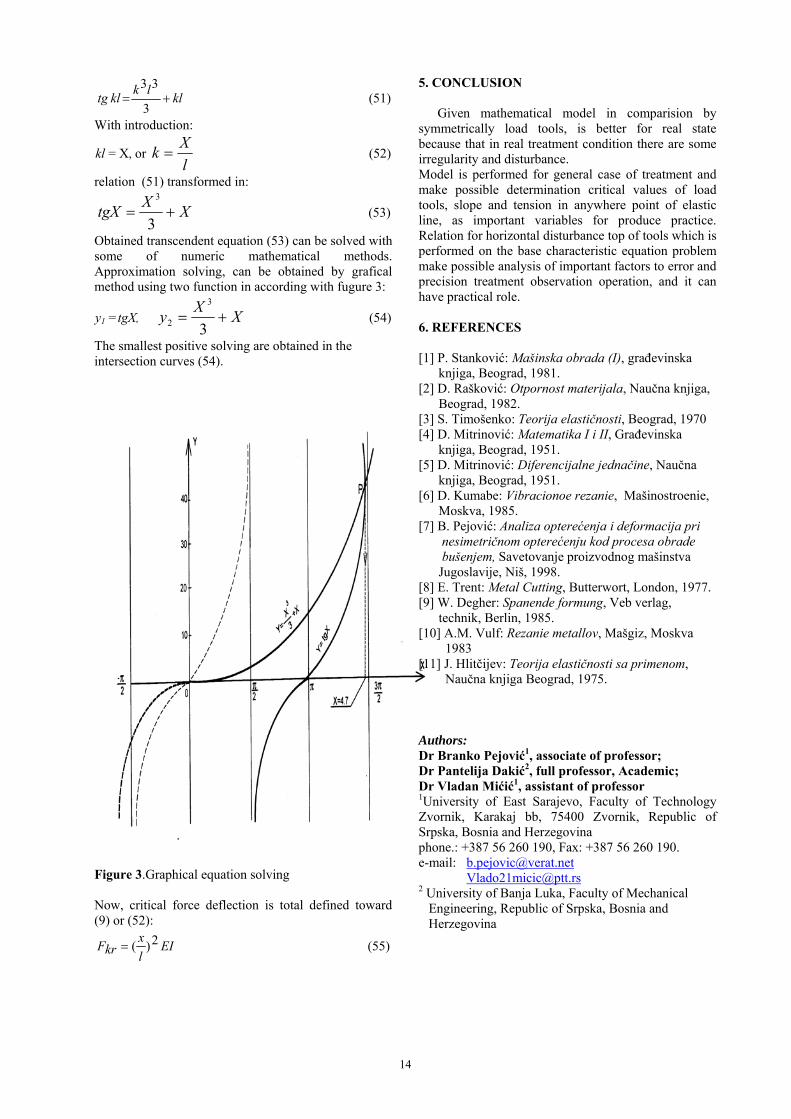
Obtained transcendent equation (53) can be solved with some of numeric mathematical methods. Approximation solving, can be obtained by grafical method using two function in according with fugure 3:
y1 =tgX, XX
y 3
3
2 (54)
The smallest positive solving are obtained in the intersection curves (54).
Figure 3.Graphical equation solving Now, critical force deflection is total defined toward (9) or (52):
EIl
xkrF 2)( (55)
5. CONCLUSION Given mathematical model in comparision by symmetrically load tools, is better for real state because that in real treatment condition there are some irregularity and disturbance. Model is performed for general case of treatment and make possible determination critical values of load tools, slope and tension in anywhere point of elastic line, as important variables for produce practice. Relation for horizontal disturbance top of tools which is performed on the base characteristic equation problem make possible analysis of important factors to error and precision treatment observation operation, and it can have practical role. 6. REFERENCES [1] P. Stanković: Mašinska obrada (I), građevinska knjiga, Beograd, 1981. [2] D. Rašković: Otpornost materijala, Naučna knjiga, Beograd, 1982. [3] S. Timošenko: Teorija elastičnosti, Beograd, 1970 [4] D. Mitrinović: Matematika I i II, Građevinska knjiga, Beograd, 1951. [5] D. Mitrinović: Diferencijalne jednačine, Naučna knjiga, Beograd, 1951. [6] D. Kumabe: Vibracionoe rezanie, Mašinostroenie, Moskva, 1985. [7] B. Pejović: Analiza opterećenja i deformacija pri nesimetričnom opterećenju kod procesa obrade bušenjem, Savetovanje proizvodnog mašinstva Jugoslavije, Niš, 1998. [8] E. Trent: Metal Cutting, Butterwort, London, 1977. [9] W. Degher: Spanende formung, Veb verlag, technik, Berlin, 1985. [10] A.M. Vulf: Rezanie metallov, Mašgiz, Moskva 1983 [11] J. Hlitčijev: Teorija elastičnosti sa primenom, Naučna knjiga Beograd, 1975. Authors: Dr Branko Pejović1, associate of professor; Dr Pantelija Dakić2, full professor, Academic; Dr Vladan Mićić1, assistant of professor 1University of East Sarajevo, Faculty of Technology Zvornik, Karakaj bb, 75400 Zvornik, Republic of Srpska, Bosnia and Herzegovina phone.: +387 56 260 190, Fax: +387 56 260 190. e-mail: [email protected] [email protected] 2 University of Banja Luka, Faculty of Mechanical Engineering, Republic of Srpska, Bosnia and Herzegovina
15
Savkovic, B., Kovac, P., Gostimirović, M., Sekulic, M., Rajnovic, D. EXPERIMENTAL STUDY OF NODULAR CAST IRON ALLOYS DURING MILLING
Abstract: In the paper experimental investigations of cutting forces during face milling are presented. Investigations were provided during milling of two type of nodular cast iron alloyed with copper. In investigations was used virtual instrumentation projected for cutting forces measurement. During investigation orthogonal cutting forces components versus time were measured and relationships for cutting forces components versus cutting conditions were determined. The chip root specimens obtained by "quick-stop" method during face milling was prepared for microstructural analysis on light and scanning electron microscopy observation by standard metallographic technique. Key words: Milling, Cutting forces, Data acquisition, Virtual instrumentation, Chip root, Nodular cast iron 1. INTRODUCTION
Cutting force (resistance) and their moments have great significance in engineering technology and general in the theory of material machining. They represent the basic categories of cutting mechanics, which means that the cutting force expresses one of the basic characteristics of the state and conduct of the process [1]
Research in the field of metal processing technology, chip removal, in most of the works, was focused on machinability of material. Machinability of material defines features of tool life, cutting forces, surface quality, cutting temperature and chip form. Having known these features, as well as important technological characteristics of the material, it is important to both the classical and the automated design of cutting process technology. In accordance with that was created a database of machinability and optimization of cutting parameters [2] Nodular cast iron is the cast iron where the graphite during the process of casting aside in the form of nodules, i.e. spheres. This form of graphite is very favorable fore cast iron and in relation to all other cast iron this type has higher strength and the highest ductility. Further thermal treatments (austempering or isothermal improvement) ductile cast iron can be obtained even better features, and the resulting material is due to its unique structure - ausferrit is called ADI (Austempered Ductile Iron). Parts made from ductile iron and ADI material are used for machines and devices that operate in extreme conditions. It is therefore necessary to know the behavior of ADI materials during various cutting conditions processing. The microstructure of ductile cast iron (NL) and the ADI material in polished and bitten state are given in Figure 1 (a-c). Graphite nodule in live are spaced evenly with the degree of sferoidization over 90% and their density from 60 to 80 nodules/mm2 and with average nodules size from 40 to 55 microns, Figure 1 (a). The microstructure of nodular cast iron metal base consists of ferrite and pearlite (mostly pearlit, with
more than 90% pearlite), Figure 1 (b). The microstructure of ADI material obtained after austempering of nodular cast iron is ausferrite with metal base, composed of acicular ferrite and austenite left, Figure 1 (c). The amount of residual austenite in the ADI microstructure material is 16.56%.
Figure 1. (a-c) The microstructure of ductile iron
castings (NL) and the ADI material a) nodule graphite, b) microstructure of NL pearlite, c) microstructure of
ADI ausferrite
Nodular cast iron and ADI mechanical properties are shown in Table 1. Austempering process improves all the mechanical properties of ductile cast iron, so it comes to enhancing the value of strength and hardness of 1.5 to 2 times. This increase in mechanical properties is caused by changing the microstructure of predominantly pearlite in the NL in ausferrite in ADI materials. Material Tensile
strength Rm[MPa]
Yield strength
Rp0.2%[MPa]
Hardness HV10
NL 771 510 270 ADI 1110 995 480
Table 1. Mechanical properties at room temperature
In Figure 2 are shown the orthogonal cutting forces in face milling process.
Face milling process like multi tooth simultaneously cutting and difference in the chip cross section that one tooth cut influenced development of variety of models for cutting force calculation. Variation in chip cross section gives difference in intensity of cutting forces and thermal load of single tooth [3].
16
Figure 2. Cutting forces during face milling
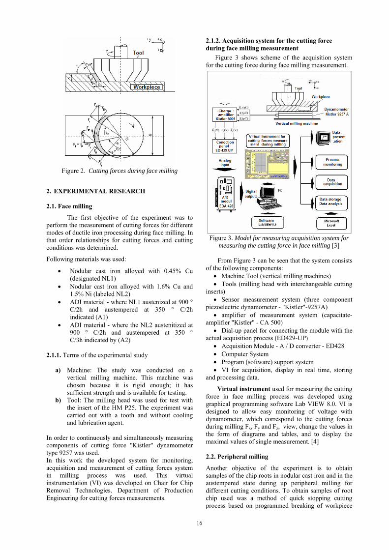
2. EXPERIMENTAL RESEARCH 2.1. Face milling
The first objective of the experiment was to perform the measurement of cutting forces for different modes of ductile iron processing during face milling. In that order relationships for cutting forces and cutting conditions was determined.
Following materials was used:
Nodular cast iron alloyed with 0.45% Cu (designated NL1)
Nodular cast iron alloyed with 1.6% Cu and 1.5% Ni (labeled NL2)
ADI material - where NL1 austenized at 900 ° C/2h and austempered at 350 ° C/2h indicated (A1)
ADI material - where the NL2 austenitized at 900 ° C/2h and austempered at 350 ° C/3h indicated by (A2)
2.1.1. Terms of the experimental study
a) Machine: The study was conducted on a vertical milling machine. This machine was chosen because it is rigid enough; it has sufficient strength and is available for testing.
b) Tool: The milling head was used for test with the insert of the HM P25. The experiment was carried out with a tooth and without cooling and lubrication agent.
In order to continuously and simultaneously measuring components of cutting force "Kistler" dynamometer type 9257 was used. In this work the developed system for monitoring, acquisition and measurement of cutting forces system in milling process was used. This virtual instrumentation (VI) was developed on Chair for Chip Removal Technologies. Department of Production Engineering for cutting forces measurements.
2.1.2. Acquisition system for the cutting force during face milling measurement
Figure 3 shows scheme of the acquisition system for the cutting force during face milling measurement.
Figure 3. Model for measuring acquisition system for
measuring the cutting force in face milling [3]
From Figure 3 can be seen that the system consists of the following components:
Machine Tool (vertical milling machines) Tools (milling head with interchangeable cutting
inserts) Sensor measurement system (three component
piezoelectric dynamometer - "Kistler"-9257A) amplifier of measurement system (capacitate-
amplifier "Kistler" - CA 500) Dial-up panel for connecting the module with the
actual acquisition process (ED429-UP) Acquisition Module - A / D converter - ED428 Computer System Program (software) support system VI for acquisition, display in real time, storing
and processing data.
Virtual instrument used for measuring the cutting force in face milling process was developed using graphical programming software Lab VIEW 8.0. VI is designed to allow easy monitoring of voltage with dynamometer, which correspond to the cutting forces during milling Fx, Fy and Fz, view, change the values in the form of diagrams and tables, and to display the maximal values of single measurement. [4] 2.2. Peripheral milling
Another objective of the experiment is to obtain samples of the chip roots in nodular cast iron and in the austempered state during up peripheral milling for different cutting conditions. To obtain samples of root chip used was a method of quick stopping cutting process based on programmed breaking of workpiece
17
materials. Thus obtained samples were used for metallographic analysis to study the process of chip formation.
2.2.1. Terms of the experimental study a) Machine: vertical milling machine
"PRVOMAJSKA" FSS GVK-3P, which was carried out and the first experimental surveys.
b) Tool: The survey was used peripheral milling cutter with screw teeth JAL 63x40x27 N made from high speed cutting steel with TiN coating.
c) Equipment for cooling and lubrication was not used.
For microstructural analysis, samples were prepared for light and scanning electron microscopy observation of the standard metallographic technique and were investigated by Leitz-Orthoplan light microscope (LM) and JEOL JSM 6460 LV scanning electron microscope (SEM) working at voltage of 25 kW. 4. RESULTS AND DISCUSSION
Measuring components of the resulting cutting force was adapted statistical methods three factorial design of the experiment, which in addition to savings in the tool, workpiece material and time trials, provide sufficient reliable dependence between input and output parameters of the process.
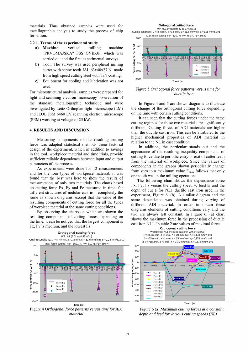
As experiments were done for 12 measurements and for the four types of workpiece material, it was found that the best was here to show the results of measurements of only two materials. The charts based on cutting force Fx, Fy and Fz measured in time, for different structures of nodular cast iron completely the same as shown diagrams, except that the value of the resulting components of cutting force for all the types of worpiece material at the same cutting conditions.
By observing the charts on which are shown the resulting components of cutting forces depending on the time, it can be noticed that the largest component is Fx, Fy is medium, and the lowest Fz.
Orthogonal cutting forceWP: A1 (ADI sa 0,45%Cu)
Cutting conditions: v =44 m/min, a =1,8 mm, s = 31,5 mm/min, s1=0,28 mm/z, z=1
Max. force cutting: Fx= -1521 N, Fy= 619 N, Fz= 350 N
-2000
-1500
-1000
-500
0
500
1000
2,8
2,8
32,
85
2,8
82
,92,
93
2,9
52,
98 3
3,0
33,
05
3,0
83
,13,
13
3,1
53,
18
3,2
3,2
33,
25
3,2
83
,33,
33
3,3
53,
38
3,4
3,4
33,
45
3,4
83
,53,
53
3,5
53,
58
3,6
3,6
33
65
Time t (s)
Fo
rce
cu
ttin
g F
x,
Fy
, F
z (N
)
Sila Fx
Sila Fy
Sila Fz
Force FxForce FyForce Fz
Figure 4 Orthogonal force patterns versus time for ADI
material
Orthogonal cutting forceWP: NL1 (nodularni liv sa 0,45%Cu)
Cutting conditions: v =44 m/min, a =1,8 mm, s = 31,5 mm/min, s1=0,28 mm/z, z=1
Max. force cutting: Fx= -1259 N, Fy= 466 N, Fz= 345 N
-1500
-1000
-500
0
500
1000
1,4
51,
47
1,5
1,5
21,
54
1,5
61,
59
1,6
11,
63
1,6
51,
68
1,7
1,7
21,
74
1,7
71,
79
1,8
11,
83
1,8
61,
88
1,9
1,9
21,
95
1,9
71,
99
2,0
12,
04
2,0
62,
08
2,1
2,1
32,
15
2,1
72,
19
Time t (s)
Fo
rce
cu
ttin
g F
x, F
y, F
z (N
)
Sila Fx
Sila Fy
Sila Fz
Force FxForce FyForce Fz
Figure 5 Orthogonal force patterns versus time for
ductile iron
In Figure 4 and 5 are shown diagrams to illustrate the change of the orthogonal cutting force depending on the time with certain cutting conditions.
It can seen that the cutting forces under the same cutting regimes for these two materials are significantly different. Cutting forces of ADI materials are higher than the ductile cast iron. This can be attributed to the higher mechanical properties of ADI material in relation to the NL in cast condition.
In addition, the particular stands out and the appearance of the resulting inequality components of cutting force due to periodic entry or exit of cutter teeth from the material of workpiece. Since the values of components in the graphs shown periodically change from zero to a maximum value Fimax follows that only one tooth was in the milling operation. The following chart shows the dependence force Fx, Fy, Fz versus the cutting speed v, feed s1 and the depth of cut a for NL1 ductile cast iron used in the experiment, Figure 6. (b). A similar diagram and the same dependence was obtained during varying of different ADI material. In order to obtain these diagrams elements of cutting conditions vary and the two are always left constant. In Figure 6. (a) chart shows the maximum force in the processing of ductile cast iron NL1. In table 2 are values of maximal force.
Orthogonal cutting forceWorkpiece: NL1 (nodular cast iron with 0,45%Cu)
1.v =44 m/min, a =1 mm, s = 20 mm/min, s1=0,178 mm/z, z=12.v =55 m/min, a =1 mm, s = 25 mm/min, s1=0,178 mm/z, z=1
3. v =71m/min, a =1 mm, s = 31,5 mm/min, s1=0,178 mm/z, z=1
Force Fx1
Force Fy1
Force Fz1
Force Fx2
Force Fy2Force Fz2
Force Fx3
Force Fy3
Force Fz3
-700
-600
-500
-400
-300
-200
-100
0
100
200
300
0 0,005 0,01 0,015 0,02 0,025 0,03 0,035 0,04
Time t (s)
Fo
rce
cu
ttin
g F
x, F
y, F
z (N
)
Sila Fx1Sila Fy1Sila Fz1
Sila Fx2Sila Fy2Sila Fz2Sila Fx3
Sila Fy3Sila Fz3
Force Fx1Force Fy1Force Fz1Force Fx2Force Fy2Force Fz2Force Fx3Force Fy3Force Fz3
Figure 6 (a) Maximum cutting forces at a constant depth and feed for various cutting speeds (NL)
18
Maximum cutting force at different cutting speeds
0
100
200
300
400
500
600
700
44 55.2 71Cutting speed [mm/min]
Fo
rce
cu
ttin
g F
x, F
y, F
z [N
]
Force FxForce FyForce Fz
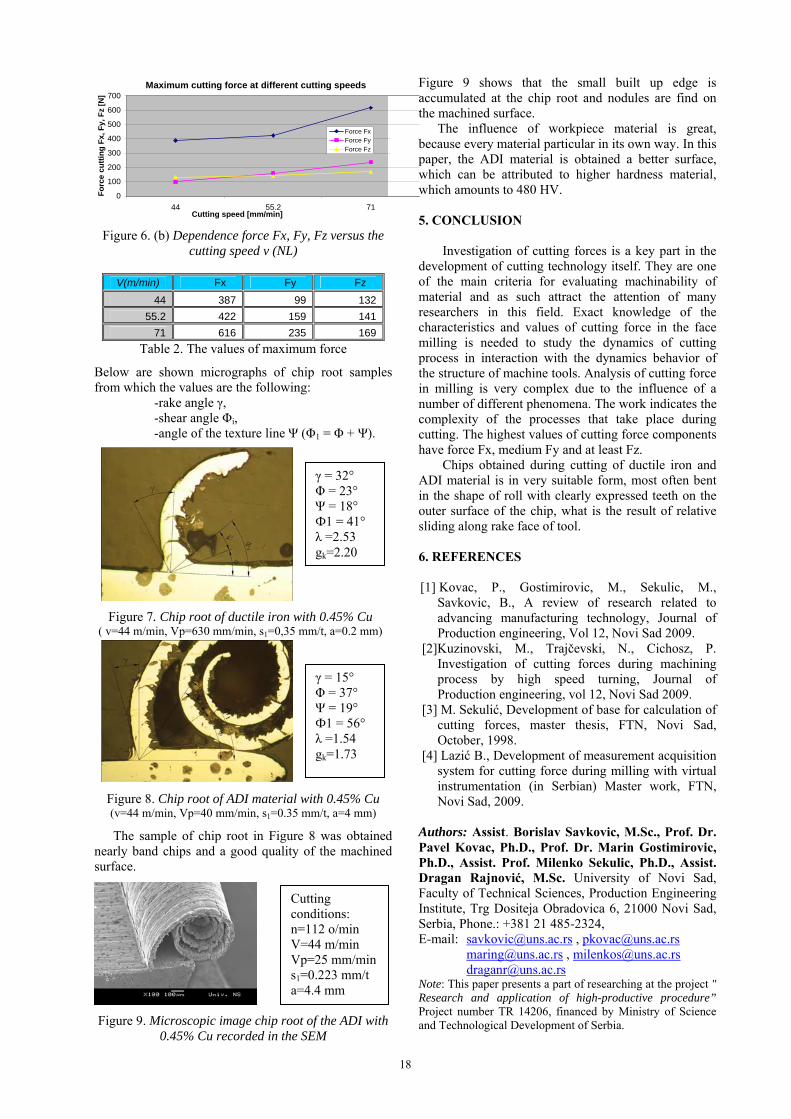
Figure 6. (b) Dependence force Fx, Fy, Fz versus the
cutting speed v (NL)
V(m/min) Fx Fy Fz
44 387 99 132
55.2 422 159 141
71 616 235 169
Table 2. The values of maximum force
Below are shown micrographs of chip root samples from which the values are the following: -rake angle γ, -shear angle Φi, -angle of the texture line Ψ (Φ1 = Φ + Ψ).
Figure 7. Chip root of ductile iron with 0.45% Cu ( v=44 m/min, Vp=630 mm/min, s1=0,35 mm/t, a=0.2 mm)
Figure 8. Chip root of ADI material with 0.45% Cu (v=44 m/min, Vp=40 mm/min, s1=0.35 mm/t, a=4 mm)
The sample of chip root in Figure 8 was obtained nearly band chips and a good quality of the machined surface.
Figure 9. Microscopic image chip root of the ADI with
0.45% Cu recorded in the SEM
Figure 9 shows that the small built up edge is accumulated at the chip root and nodules are find on the machined surface. The influence of workpiece material is great, because every material particular in its own way. In this paper, the ADI material is obtained a better surface, which can be attributed to higher hardness material, which amounts to 480 HV. 5. CONCLUSION
Investigation of cutting forces is a key part in the development of cutting technology itself. They are one of the main criteria for evaluating machinability of material and as such attract the attention of many researchers in this field. Exact knowledge of the characteristics and values of cutting force in the face milling is needed to study the dynamics of cutting process in interaction with the dynamics behavior of the structure of machine tools. Analysis of cutting force in milling is very complex due to the influence of a number of different phenomena. The work indicates the complexity of the processes that take place during cutting. The highest values of cutting force components have force Fx, medium Fy and at least Fz.
Chips obtained during cutting of ductile iron and ADI material is in very suitable form, most often bent in the shape of roll with clearly expressed teeth on the outer surface of the chip, what is the result of relative sliding along rake face of tool. 6. REFERENCES
[1] Kovac, P., Gostimirovic, M., Sekulic, M., Savkovic, B., A review of research related to advancing manufacturing technology, Journal of Production engineering, Vol 12, Novi Sad 2009.
[2]Kuzinovski, М., Тrajčevski, N., Cichosz, P. Investigation of cutting forces during machining process by high speed turning, Journal of Production engineering, vol 12, Novi Sad 2009.
[3] M. Sekulić, Development of base for calculation of cutting forces, master thesis, FTN, Novi Sad, October, 1998.
[4] Lazić B., Development of measurement acquisition system for cutting force during milling with virtual instrumentation (in Serbian) Master work, FTN, Novi Sad, 2009.
Authors: Assist. Borislav Savkovic, M.Sc., Prof. Dr. Pavel Kovac, Ph.D., Prof. Dr. Marin Gostimirovic, Ph.D., Assist. Prof. Milenko Sekulic, Ph.D., Assist. Dragan Rajnović, M.Sc. University of Novi Sad, Faculty of Technical Sciences, Production Engineering Institute, Trg Dositeja Obradovica 6, 21000 Novi Sad, Serbia, Phone.: +381 21 485-2324, E-mail: [email protected] , [email protected] [email protected] , [email protected] [email protected] Note: This paper presents a part of researching at the project " Research and application of high-productive procedure” Project number TR 14206, financed by Ministry of Science and Technological Development of Serbia.
γ = 32° Φ = 23° Ψ = 18° Ф1 = 41° λ =2.53 gk=2.20
γ = 15° Φ = 37° Ψ = 19° Ф1 = 56° λ =1.54 gk=1.73
Cutting conditions: n=112 o/min V=44 m/min Vp=25 mm/min s1=0.223 mm/t a=4.4 mm
19
Sekulić, M., Kovač, P., Gostimirović, M., Jurković, Z., Savković, B.
A NEW THRUST FORCE MODEL FOR DRILLING PROCESS
Abstract: This paper presents a new model for drilling process. The key to the model is the decomposition of the drilling process. The thrust force acting on drill is the sum of three components: the cutting component, the thrust force attributed to ploughing at the chisel edge and the thrust force resulting from friction at the margin. The thrust force structure is determined by experimental decomposition of the drilling process. The result of the simulation study has shown a very good agreement between the theoretical predictions and experimental evidence. Key words: drilling, thrust force 1. INTRODUCTION Drilling is the most commonly used machining operation. However, it is also one of the most complex cutting processes. The fact the great majority of hole diameters are within the 10 to 20 mm range cannot be efficiency produced by any other way, clearly shows how important the drilling operation is in the field of modern metal cutting. In the study of the drilling process, modeling is very important as it helps us to understand the process and hence, to solve practical problems such as chatter and tool breakage. According to the literature, there are at least 10 different drilling process models. The basic principles of drilling are now well understood. The typical cutting process of a twist drill is three-dimensional and oblique. Cutting speed, inclination angle and rake angle vary depending on the radius r along the cutting lip of the drill. Cutting characteristics of the drilling process are fundamentally nonlinear because of the complex physical phenomena of built-up edges, temperature variations, strain hardening and tool wear. The thrust force depends on the geometry of the drill (diameter, point angle, lip length, evolution of the cutting angles along the edges, etc.) as well as on the cutting conditions (cutting speed, feed rate, lubrication, etc.) and on the material’s properties. It is known that a drill consists of two cutting edges: the chisel edge and the main cutting edges. The point of the drill is generally formed by a chisel edge, which has a highly negative rake angle and very low cutting speeds because of its small radius. The cutting speed of the chisel edge is, in fact, zero at the drill center. The main feature that distinguishes it from other processes is the fact that cutting is combined with extrusion in the centre of the drill, at the chisel edge. The chisel edge extrudes into the workpiece material and hence, contributes substantially to the thrust force but little to the torque. Also, it is rather difficult to explain its cutting action on a theoretical basis, as there is an oblique cutting action combined with an extrusion process which produces two distinct types of chips, as shown in Figure 1. The experimental investigation by Oxford showed that
during cutting there were three identifiable zones of interest at the drill point, namely, the main cutting edges (or lips), the secondary cutting edges on the chisel edge, and an indentation zone about the drill centre, Figure 2. Outside indentation zone, the chisel edge produces an orthogonal cut with a negative rake angle, Figure 3. The rake angle is negative in the middle area and becomes gradually positive in the peripheral region. Means during drilling, the material is indented, extruded and machined by orthogonal cutting on the chisel edge and machined by oblique cutting on the main cutting edges. In drilling, the thrust force does not contain only components of the main cutting edges, also it contains some of additional loads, which is present in drilling like:
Friction force on drill edge between facet and machined hole,
Extrusion force of the chisel edge.
Fig. 1. Two types of chips that are produced by
extrusion and cutting actions in the drilling process [1]
Fig. 2. Regions of the chisel edge [1]
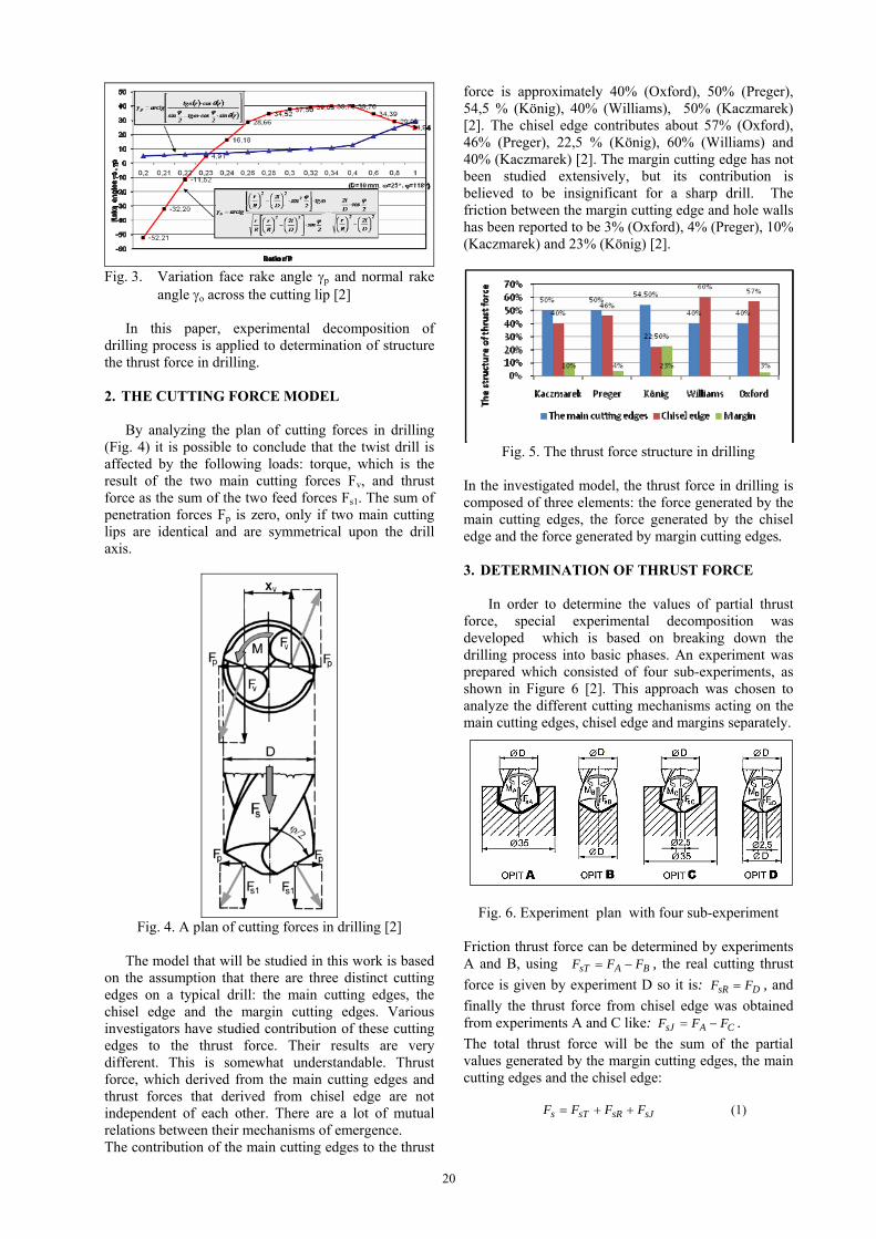
20
Fig. 3. Variation face rake angle p and normal rake
angle o across the cutting lip [2] In this paper, experimental decomposition of drilling process is applied to determination of structure the thrust force in drilling. 2. THE CUTTING FORCE MODEL By analyzing the plan of cutting forces in drilling (Fig. 4) it is possible to conclude that the twist drill is affected by the following loads: torque, which is the result of the two main cutting forces Fv, and thrust force as the sum of the two feed forces Fs1. The sum of penetration forces Fp is zero, only if two main cutting lips are identical and are symmetrical upon the drill axis.
Fig. 4. A plan of cutting forces in drilling [2]
The model that will be studied in this work is based on the assumption that there are three distinct cutting edges on a typical drill: the main cutting edges, the chisel edge and the margin cutting edges. Various investigators have studied contribution of these cutting edges to the thrust force. Their results are very different. This is somewhat understandable. Thrust force, which derived from the main cutting edges and thrust forces that derived from chisel edge are not independent of each other. There are a lot of mutual relations between their mechanisms of emergence. The contribution of the main cutting edges to the thrust
force is approximately 40% (Oxford), 50% (Preger), 54,5 % (König), 40% (Williams), 50% (Kaczmarek) [2]. The chisel edge contributes about 57% (Oxford), 46% (Preger), 22,5 % (König), 60% (Williams) and 40% (Kaczmarek) [2]. The margin cutting edge has not been studied extensively, but its contribution is believed to be insignificant for a sharp drill. The friction between the margin cutting edge and hole walls has been reported to be 3% (Oxford), 4% (Preger), 10% (Kaczmarek) and 23% (König) [2].
Fig. 5. The thrust force structure in drilling
In the investigated model, the thrust force in drilling is composed of three elements: the force generated by the main cutting edges, the force generated by the chisel edge and the force generated by margin cutting edges. 3. DETERMINATION OF THRUST FORCE In order to determine the values of partial thrust force, special experimental decomposition was developed which is based on breaking down the drilling process into basic phases. An experiment was prepared which consisted of four sub-experiments, as shown in Figure 6 [2]. This approach was chosen to analyze the different cutting mechanisms acting on the main cutting edges, chisel edge and margins separately.
Fig. 6. Experiment plan with four sub-experiment
Friction thrust force can be determined by experiments A and B, using BAsT FFF , the real cutting thrust
force is given by experiment D so it is: DsR FF , and
finally the thrust force from chisel edge was obtained from experiments A and C like: CAsJ FFF .
The total thrust force will be the sum of the partial values generated by the margin cutting edges, the main cutting edges and the chisel edge:
sJsRsTs FFFF (1)
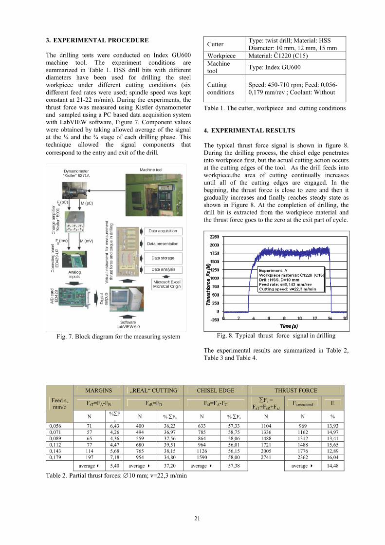
21
3. EXPERIMENTAL PROCEDURE The drilling tests were conducted on Index GU600 machine tool. The experiment conditions are summarized in Table 1. HSS drill bits with different diameters have been used for drilling the steel workpiece under different cutting conditions (six different feed rates were used; spindle speed was kept constant at 21-22 m/min). During the experiments, the thrust force was measured using Kistler dynamometer and sampled using a PC based data acquisition system with LabVIEW software, Figure 7. Component values were obtained by taking allowed average of the signal at the ¼ and the ¾ stage of each drilling phase. This technique allowed the signal components that correspond to the entry and exit of the drill.
Machine toolDynamometer“Kistler” 9271A
Ch
arge
am
plif
ier
“Kis
tler”
500
1C
one
ctin
g pa
nel
ED
42
9-U
PA
/D c
ard
ED
428
F (pC)s
F mV( )s
M (pC)
M (mV)
Analoginputs
Dig
ital
outp
uts
SoftwareLabVIEW 6.0
Data acquisition
Data presentation
Data storage
Data analysis
Microsoft ExcelMicroCal Origin
Vir
tua
l in
stru
men
t fo
r m
easu
rem
ent
th
rust
for
ce a
nd
torq
ue
in d
rillin
g
Fig. 7. Block diagram for the measuring system
Cutter Type: twist drill; Material: HSS Diameter: 10 mm, 12 mm, 15 mm
Workpiece Material: Č1220 (C15) Machine tool
Type: Index GU600
Cutting conditions
Speed: 450-710 rpm; Feed: 0,056-0,179 mm/rev ; Coolant: Without
Table 1. The cutter, workpiece and cutting conditions 4. EXPERIMENTAL RESULTS The typical thrust force signal is shown in figure 8. During the drilling process, the chisel edge penetrates into workpiece first, but the actual cutting action occurs at the cutting edges of the tool. As the drill feeds into workpiece,the area of cutting continually increases until all of the cutting edges are engaged. In the begining, the thrust force is close to zero and then it gradually increases and finally reaches steady state as shown in Figure 8. At the completion of drilling, the drill bit is extracted from the workpiece material and the thrust force goes to the zero at the exit part of cycle.
Fig. 8. Typical thrust force signal in drilling
The experimental results are summarized in Table 2, Table 3 and Table 4.
MARGINS „REAL“ CUTTING CHISEL EDGE THRUST FORCE
FsT=FA-FB FsR=FD FsJ=FA-FC Fs =
FsT+FsR+FsJ Fs.measured E Feed s,
mm/o
N %Fs
N % Fs N % Fs N N %
0,056 71 6,43 400 36,23 633 57,33 1104 969 13,93 0,071 57 4,26 494 36,97 785 58,75 1336 1162 14,97 0,089 65 4,36 559 37,56 864 58,06 1488 1312 13,41 0,112 77 4,47 680 39,51 964 56,01 1721 1488 15,65 0,143 114 5,68 765 38,15 1126 56,15 2005 1776 12,89 0,179 197 7,18 954 34,80 1590 58,00 2741 2362 16,04
average 5,40 average 37,20 average 57,38 average 14,48
Table 2. Partial thrust forces: 10 mm; v=22,3 m/min
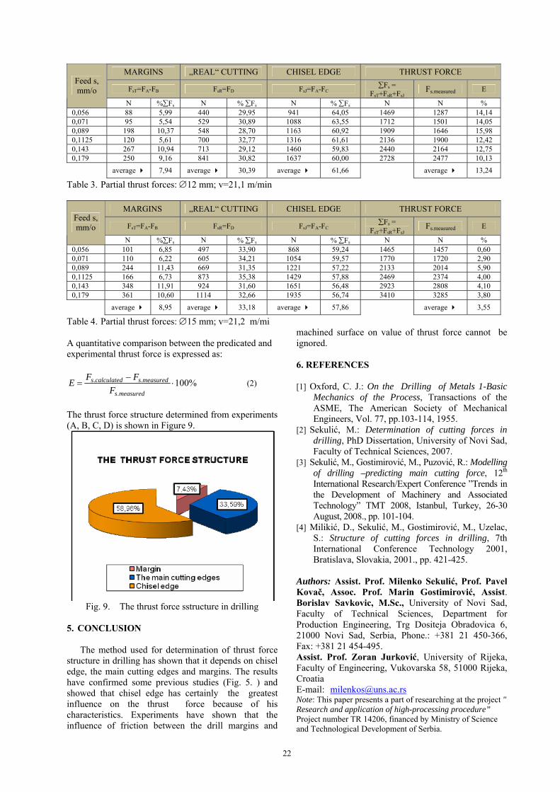
22
MARGINS „REAL“ CUTTING CHISEL EDGE THRUST FORCE
FsT=FA-FB FsR=FD FsJ=FA-FC Fs =
FsT+FsR+FsJ Fs.measured E
Feed s, mm/o
N %Fs N % Fs N % Fs N N % 0,056 88 5,99 440 29,95 941 64,05 1469 1287 14,14 0,071 95 5,54 529 30,89 1088 63,55 1712 1501 14,05 0,089 198 10,37 548 28,70 1163 60,92 1909 1646 15,98 0,1125 120 5,61 700 32,77 1316 61,61 2136 1900 12,42 0,143 267 10,94 713 29,12 1460 59,83 2440 2164 12,75 0,179 250 9,16 841 30,82 1637 60,00 2728 2477 10,13
average 7,94 average 30,39 average 61,66 average 13,24
Table 3. Partial thrust forces: 12 mm; v=21,1 m/min
MARGINS „REAL“ CUTTING CHISEL EDGE THRUST FORCE
FsT=FA-FB FsR=FD FsJ=FA-FC Fs =
FsT+FsR+FsJ Fs.measured E
Feed s, mm/o
N %Fs N % Fs N % Fs N N % 0,056 101 6,85 497 33,90 868 59,24 1465 1457 0,60 0,071 110 6,22 605 34,21 1054 59,57 1770 1720 2,90 0,089 244 11,43 669 31,35 1221 57,22 2133 2014 5,90 0,1125 166 6,73 873 35,38 1429 57,88 2469 2374 4,00 0,143 348 11,91 924 31,60 1651 56,48 2923 2808 4,10 0,179 361 10,60 1114 32,66 1935 56,74 3410 3285 3,80
average 8,95 average 33,18 average 57,86 average 3,55
Table 4. Partial thrust forces: 15 mm; v=21,2 m/mi A quantitative comparison between the predicated and experimental thrust force is expressed as:
%100.
..
measureds
measuredscalculateds
F
FFE (2)
The thrust force structure determined from experiments (A, B, C, D) is shown in Figure 9.
Fig. 9. The thrust force sstructure in drilling
5. CONCLUSION The method used for determination of thrust force structure in drilling has shown that it depends on chisel edge, the main cutting edges and margins. The results have confirmed some previous studies (Fig. 5. ) and showed that chisel edge has certainly the greatest influence on the thrust force because of his characteristics. Experiments have shown that the influence of friction between the drill margins and
machined surface on value of thrust force cannot be ignored. 6. REFERENCES [1] Oxford, C. J.: On the Drilling of Metals 1-Basic
Mechanics of the Process, Transactions of the ASME, The American Society of Mechanical Engineers, Vol. 77, pp.103-114, 1955.
[2] Sekulić, M.: Determination of cutting forces in drilling, PhD Dissertation, University of Novi Sad, Faculty of Technical Sciences, 2007.
[3] Sekulić, M., Gostimirović, M., Puzović, R.: Modelling of drilling –predicting main cutting force, 12th International Research/Expert Conference ”Trends in the Development of Machinery and Associated Technology” TMT 2008, Istanbul, Turkey, 26-30 August, 2008., pp. 101-104.
[4] Milikić, D., Sekulić, M., Gostimirović, M., Uzelac, S.: Structure of cutting forces in drilling, 7th International Conference Technology 2001, Bratislava, Slovakia, 2001., pp. 421-425.
Authors: Assist. Prof. Milenko Sekulić, Prof. Pavel Kovač, Assoc. Prof. Marin Gostimirović, Assist. Borislav Savkovic, M.Sc., University of Novi Sad, Faculty of Technical Sciences, Department for Production Engineering, Trg Dositeja Obradovica 6, 21000 Novi Sad, Serbia, Phone.: +381 21 450-366, Fax: +381 21 454-495. Assist. Prof. Zoran Jurković, University of Rijeka, Faculty of Engineering, Vukovarska 58, 51000 Rijeka, Croatia E-mail: [email protected] Note: This paper presents a part of researching at the project " Research and application of high-processing procedure” Project number TR 14206, financed by Ministry of Science and Technological Development of Serbia.
23
Cep, R., Sadilek, M., Kouril, K., Budak, I., Hadzistevic, M.
TESTING OF MACHINE TOOL ACCURACY BY THE QC10 BALLBAR SYSTEM Abstract: For machining more complicated parts, above all in lump and small-lot productions, such as production in tool works, it is of advantage to use CNC machine tools. A very important condition for exact machining is the machine tool stability in order to keep high accuracy of its programmed (in most cases non-linear) path. The following text deals with this accuracy detection, it describes particular tests carried out in toolshed RIETER Elitex Inc. Hnatnice in Czech Republic. Key words: dynamic accuracy, machine tool, testing 1. INTRODUCTION It is impossible to ensure the required speed, surface finish and first of all production operability by the traditional tooling method. It is also impossible to ensure the needed functional surface accuracy in that way. It is even impossible to size some surfaces by this technology. Therefore a new HSC (High Speed Cutting) technology is introduced. This new method successfully solves problems of the traditional cutting technology of 3D surfaces. One of the possibilities how to reduce the prime costs, operation times and to improve constructional parts quality nowadays in the splintery cutting area displays cutting high rate [1]. By this technology it is possible to shape thoroughly without hand-made finalization. This is enabled only by using computer techniques with top CAD/CAM systems. It is necessary to start a close cooperation between companies producing machinery or tools, users and companies offering CAD/CAM systems. Characteristics of HSC cutting:
high cutting speed high feed speed temperature rise in the cut point smaller warming-up of work piece better surface finish major formative accuracy and position
accuracy high efficiency great operational safety
In the development of the machine for splintery cutting, producers´ obvious effort can be seen to increase labour productivity and to achieve a higher machined surface quality. A significant progress has been recently made especially in terms of the main times, which have no small influence on prices of manufactured parts. Good results were achieved especially by the development of new cutting materials, which demand high feed values for optimal cutting conditions. To match technological requirements, not
only high feed speeds are required, but also their high dynamics and high speed of the spindle. An obvious requirement is the high stiffness of the whole machinery and especially of the feed mechanisms. Mechanized 3D surfaces often contain complicated and mathematically indefinable surfaces and preparation of the programs for their cutting on NC machines is possible practically only while using CAD programs. These way generated programs are demanding on memory size and on speed and quality of information processing in the control system. CNC systems fit for HSC cutting are equipped with circuits of re-contouring prediction (Look Ahead) that checks the speed with regard to the shape strain of the cutting surface. Their task is to operate the feed speed in order not to make formative mistakes on sharp angles and edges [2].
If we summarize the introduced demands on the high-speed cutting, these items are concerned:
cutting materials for achievement of high cutting speeds
high - speed spindles feed mechanisms enabling high feeds and high
acceleration high stiffness of the whole system: machine -
tool – work piece CNC control systems with high speed of
block processing and with Look Ahead function
2. EXPERIMENTAL PART 2.1 Tested machine tool
Measuring was carried out on a machine-tool WHN 13 CNC produced by TOS Varnsdorf Inc. It is a horizontal milling machine with a cruciate make-up of beds, a lengthwise adjustable stand, a telescopic spindle and a crosswise adjustable rotary desk. Module construction offers wide range of variations in all the parameters. It is also equipped with digitally controlled AC propellants SIEMENS and a control system
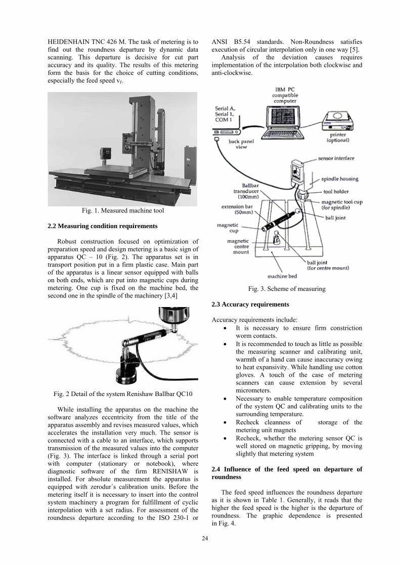
24
HEIDENHAIN TNC 426 M. The task of metering is to find out the roundness departure by dynamic data scanning. This departure is decisive for cut part accuracy and its quality. The results of this metering form the basis for the choice of cutting conditions, especially the feed speed vf.
Fig. 1. Measured machine tool
2.2 Measuring condition requirements Robust construction focused on optimization of preparation speed and design metering is a basic sign of apparatus QC – 10 (Fig. 2). The apparatus set is in transport position put in a firm plastic case. Main part of the apparatus is a linear sensor equipped with balls on both ends, which are put into magnetic cups during metering. One cup is fixed on the machine bed, the second one in the spindle of the machinery [3,4]
Fig. 2 Detail of the system Renishaw Ballbar QC10
While installing the apparatus on the machine the
software analyzes eccentricity from the title of the apparatus assembly and revises measured values, which accelerates the installation very much. The sensor is connected with a cable to an interface, which supports transmission of the measured values into the computer (Fig. 3). The interface is linked through a serial port with computer (stationary or notebook), where diagnostic software of the firm RENISHAW is installed. For absolute measurement the apparatus is equipped with zerodur´s calibration units. Before the metering itself it is necessary to insert into the control system machinery a program for fulfillment of cyclic interpolation with a set radius. For assessment of the roundness departure according to the ISO 230-1 or
ANSI B5.54 standards. Non-Roundness satisfies execution of circular interpolation only in one way [5]. Analysis of the deviation causes requires implementation of the interpolation both clockwise and anti-clockwise.
Fig. 3. Scheme of measuring
2.3 Accuracy requirements Accuracy requirements include:
It is necessary to ensure firm constriction worm contacts.
It is recommended to touch as little as possible the measuring scanner and calibrating unit, warmth of a hand can cause inaccuracy owing to heat expansivity. While handling use cotton gloves. A touch of the case of metering scanners can cause extension by several micrometers.
Necessary to enable temperature composition of the system QC and calibrating units to the surrounding temperature.
Recheck cleanness of storage of the metering unit magnets
Recheck, whether the metering sensor QC is well stored on magnetic gripping, by moving slightly that metering system
2.4 Influence of the feed speed on departure of roundness The feed speed influences the roundness departure as it is shown in Table 1. Generally, it reads that the higher the feed speed is the higher is the departure of roundness. The graphic dependence is presented in Fig. 4.
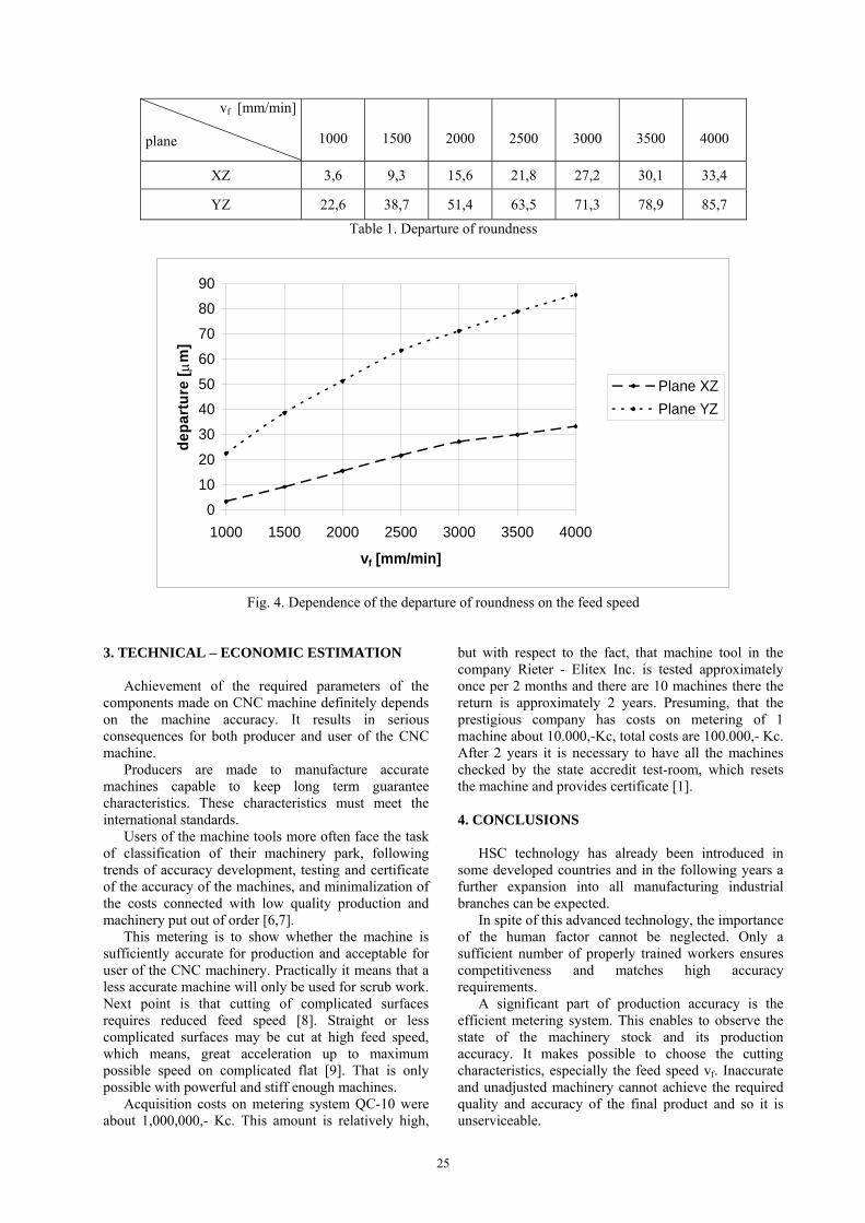
25
vf [mm/min]
plane
1000
1500
2000
2500
3000
3500
4000
XZ 3,6 9,3 15,6 21,8 27,2 30,1 33,4
YZ 22,6 38,7 51,4 63,5 71,3 78,9 85,7
Table 1. Departure of roundness
0
10
20
30
40
50
60
70
80
90
1000 1500 2000 2500 3000 3500 4000
vf [mm/min]
de
pa
rtu
re [m
]
Plane XZ
Plane YZ
Fig. 4. Dependence of the departure of roundness on the feed speed
3. TECHNICAL – ECONOMIC ESTIMATION Achievement of the required parameters of the components made on CNC machine definitely depends on the machine accuracy. It results in serious consequences for both producer and user of the CNC machine. Producers are made to manufacture accurate machines capable to keep long term guarantee characteristics. These characteristics must meet the international standards.
Users of the machine tools more often face the task of classification of their machinery park, following trends of accuracy development, testing and certificate of the accuracy of the machines, and minimalization of the costs connected with low quality production and machinery put out of order [6,7]. This metering is to show whether the machine is sufficiently accurate for production and acceptable for user of the CNC machinery. Practically it means that a less accurate machine will only be used for scrub work. Next point is that cutting of complicated surfaces requires reduced feed speed [8]. Straight or less complicated surfaces may be cut at high feed speed, which means, great acceleration up to maximum possible speed on complicated flat [9]. That is only possible with powerful and stiff enough machines.
Acquisition costs on metering system QC-10 were about 1,000,000,- Kc. This amount is relatively high,
but with respect to the fact, that machine tool in the company Rieter - Elitex Inc. is tested approximately once per 2 months and there are 10 machines there the return is approximately 2 years. Presuming, that the prestigious company has costs on metering of 1 machine about 10.000,-Kc, total costs are 100.000,- Kc. After 2 years it is necessary to have all the machines checked by the state accredit test-room, which resets the machine and provides certificate [1].
4. CONCLUSIONS
HSC technology has already been introduced in some developed countries and in the following years a further expansion into all manufacturing industrial branches can be expected.
In spite of this advanced technology, the importance of the human factor cannot be neglected. Only a sufficient number of properly trained workers ensures competitiveness and matches high accuracy requirements. A significant part of production accuracy is the efficient metering system. This enables to observe the state of the machinery stock and its production accuracy. It makes possible to choose the cutting characteristics, especially the feed speed vf. Inaccurate and unadjusted machinery cannot achieve the required quality and accuracy of the final product and so it is unserviceable.

26
5. REFERENCES [1] Čep, R.: Influence of cutting conditions to
production accuracy at machining of 3D surfaces (in Czech). Diploma thesis. Ostrava, VŠB-TU, 2000, 46 p.
[2] Machalínek, M.: Trend is high speed cutting (in Czech). Technický týdeník 24/1998, str. 6-7.
[3] Stević, M., Hodolič, J., Vrečić, T.: Primena BALLBAR QC10 sistema, Zbornik radova, IX Međunarodna naučno-stručna konferencija Fleksibilne tehnologije MMA 2006, Ćosić, I. (Ed), ISBN 86-85211-96-4, pp. 51-52, Univerzitet u Novom Sadu, Fakultet tehničkih nauka – Institut za proizvodno mašinstvo, 15. - 16. Jun, Novi Sad, Srbija i Crna Gora, 2006.
[4] Cedilnik, M., Soković, M., Jurkovič, J. Umerjanje in preverjanje geometrijske natančnosti računalniško krmiljenih obdelovalnih strojev = Calibration and checking the geometrical accuracy of a CNC machine-tool. Stroj. vestn., 2006, letn. 52, št. 11, str. 752-762. [COBISS.SI-ID 9780251], [WoS, št. citatov do 7.2.07: 0, brez avtocitatov: 0, normirano št. citatov: 0]
[5] -----: Manuál to system QC-10 BALLBAR SYSTEM v 4.21., RENISHAW.
[6] Dobránsky, J., Hatala, M.: Influence of selected technological parameter to quality parameters by injection moulding. In: Annals of DAAAM for 2007 & proceedings of the 18th International DAAAM Symposium : Intelligent Manufacturing & Automation: Focus on Creativity, Responsibility, and Ethics of Engineers : 24-27th October 2007, Zadar, Croatia. Vienna : DAAAM International, 2007. 2 p. ISBN 3-901509-58-5.
[7] Mrkvica, I., Uhlář, V.: Počáteční kontakt břitu nástroje při frézování. In. Sborník referátů VIII. mezinárodní konference Nové smery ve výrobných technologiích 2006. Prešov: Technická univerzita v Košicích, Fakulta výrobních technologií se sídlem v Prešově, 2006, s. 101-104. ISBN 80-8073-554-9.
[8] Panda, A., Jurko, J., Pandová, I, Zajac, J.: Vývoj, výroba a overenie nových výrobkov pre automobilový priemysel. 1. časť. Monografia, FVT TU Košice so sídlom v Prešove, 2009, 67 strán, ISBN 978–80–553–0149–5.
[9] Monková, K., Monka, P.: Digitalizácia dokumentácie. In: Technika. č. 12 (2004), s. 31.
Authors: Robert Cep, Ph.D., MSc. Marek Sadilek, Ph.D., MSc., VSB - Technical University of Ostrava, Faculty of Mechanical Engineering, Department of Machining and Assembly, 17. Listopadu 15/2172, 708 33 Ostrava, Czech Republic, Phone +420 59 732 3193, E-mail: [email protected] [email protected]. Karel Kouril, Ph.D., MSc. - Brno University of Technology, Faculty of Mechanical Engineering, Institute of Manufacturing Technology, Department of Machining, Technicka 2, 616 69 Brno, Czech Republic, Phone +420 54 114 2486, E-mail: [email protected] Dr Igor Budak, Assoc. prof. dr Miodrag Hadzistevic - University of Novi Sad, Faculty of Technical Sciences, Trg Dositeja Obradovica 6, 21000 Novi Sad, Serbia, Phone: +381 21 485-2255 E-mail: [email protected] [email protected]
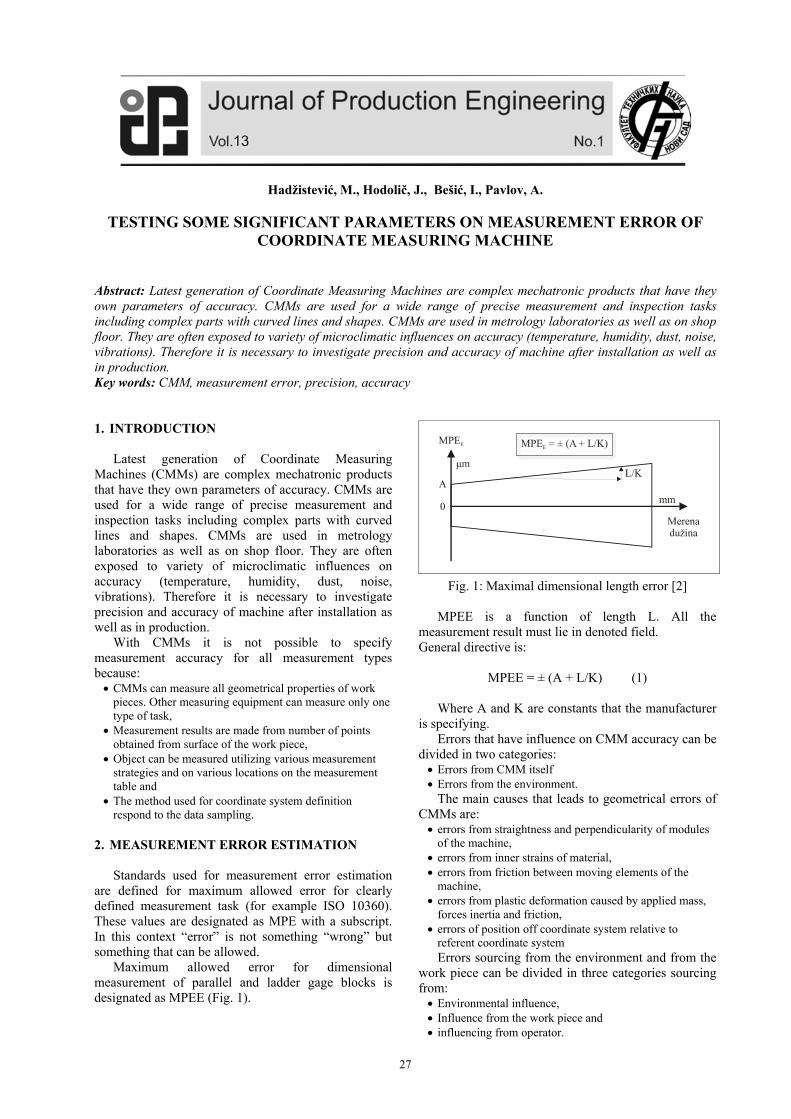
27
Hadžistević, M., Hodolič, J., Bešić, I., Pavlov, A.
TESTING SOME SIGNIFICANT PARAMETERS ON MEASUREMENT ERROR OF COORDINATE MEASURING MACHINE
Abstract: Latest generation of Coordinate Measuring Machines are complex mechatronic products that have they own parameters of accuracy. CMMs are used for a wide range of precise measurement and inspection tasks including complex parts with curved lines and shapes. CMMs are used in metrology laboratories as well as on shop floor. They are often exposed to variety of microclimatic influences on accuracy (temperature, humidity, dust, noise, vibrations). Therefore it is necessary to investigate precision and accuracy of machine after installation as well as in production. Key words: CMM, measurement error, precision, accuracy 1. INTRODUCTION Latest generation of Coordinate Measuring Machines (CMMs) are complex mechatronic products that have they own parameters of accuracy. CMMs are used for a wide range of precise measurement and inspection tasks including complex parts with curved lines and shapes. CMMs are used in metrology laboratories as well as on shop floor. They are often exposed to variety of microclimatic influences on accuracy (temperature, humidity, dust, noise, vibrations). Therefore it is necessary to investigate precision and accuracy of machine after installation as well as in production. With CMMs it is not possible to specify measurement accuracy for all measurement types because: CMMs can measure all geometrical properties of work
pieces. Other measuring equipment can measure only one type of task,
Measurement results are made from number of points obtained from surface of the work piece,
Object can be measured utilizing various measurement strategies and on various locations on the measurement table and
The method used for coordinate system definition respond to the data sampling.
2. MEASUREMENT ERROR ESTIMATION Standards used for measurement error estimation are defined for maximum allowed error for clearly defined measurement task (for example ISO 10360). These values are designated as MPE with a subscript. In this context “error” is not something “wrong” but something that can be allowed. Maximum allowed error for dimensional measurement of parallel and ladder gage blocks is designated as MPEE (Fig. 1).
Fig. 1: Maximal dimensional length error [2]
MPEE is a function of length L. All the measurement result must lie in denoted field. General directive is:
MPEE = ± (A + L/K) (1)
Where A and K are constants that the manufacturer is specifying. Errors that have influence on CMM accuracy can be divided in two categories: Errors from CMM itself Errors from the environment.
The main causes that leads to geometrical errors of CMMs are: errors from straightness and perpendicularity of modules
of the machine, errors from inner strains of material, errors from friction between moving elements of the
machine, errors from plastic deformation caused by applied mass,
forces inertia and friction, errors of position off coordinate system relative to
referent coordinate system Errors sourcing from the environment and from the work piece can be divided in three categories sourcing from: Environmental influence, Influence from the work piece and influencing from operator.
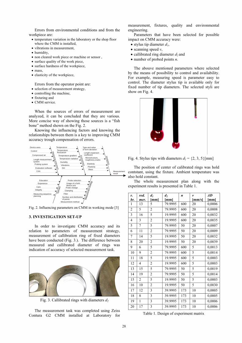
28
Errors from environmental conditions and from the workpiece are: temperature variation in the laboratory or the shop floor
where the CMM is installed, vibrations in measurement, humidity, non cleared work piece or machine or sensor , surface quality of the work piece, surface hardness of the workpiece, mass, elasticity of the workpiece,
Errors from the operator point are: selection of measurement strategy, controlling the machine, fixturing and CMM service.
When the sources of errors of measurement are analyzed, it can be concluded that they are various. More concise way of showing those sources is a “fish bone” method shown on the Fig. 2. Knowing the influencing factors and knowing the relationships between them is a key to improving CMM accuracy trough compensation of errors.
Device axes
Compressed air
Length measurementsystem
Probing system
Evaluation software
CAA
Control
Temperature
Temperaturefluctuacion
Temperature radiation
Humidity
Vibrations
Dirt
Temperature gradient
Type and valueof form deviation
Length expansioncoefficient
Microstructure,roughness,cracks
Elasticity
PlasticityMass
Measuring instrum
ent
Environm
ent
Workpiece
Usage of a forthdevice axis
Clamping
Number and distributionof points
Probe selection
Experience
Probe changeIntegrity
Measuring sequenceplanning
Education
Care
Measurement method
Filter
Measurementresult
Fig. 2. Influencing parameters on CMM in working mode [3] 3. INVESTIGATION SET-UP In order to investigate CMM accuracy and its relation to parameters of measurement strategy, measurement of callibration ring of fixed diameters have been conducted (Fig. 3.). The difference between measured and callibrated diameter of rings was indication of accuracy of selected measurement task.
Fig. 3. Callibrated rings with diameters d2
The measurement task was completed using Zeiss Contura G2 CMM installed at Laboratory for
measurement, fixtures, quality and environmental engineering. Parameters that have been selected for possible impact on CMM accuracy were: stylus tip diameter d1, scanning speed v, callibrated ring diameter d2 and number of probed points n.
The abouve mentioned parameters where selected by the means of possibility to control and availability. For example, measuring speed is parameter easy to control. The diameter stylus tip is available only for fixed number of tip diameters. The selected styli are show on Fig. 4.
Fig. 4. Stylus tips with diameters d1 = {2, 3, 5}[mm] The position of center of calibrated rings was hold contstant, using the fixture. Ambient temperature was also hold constant. The whole measurement plan along with the experiment results is presented in Table 1.
r. br.
red.mer.
d1 [mm]
d2 [mm]
n v [mm/s]
ΔD [mm]
1 13 5 79.9995 600 20 0,0006
2 5 2 79.9995 600 20 0,0008
3 16 5 19.9995 600 20 0,0032
4 3 2 19.9995 600 20 0,0035
5 7 5 79.9995 50 20 0,0007
6 11 2 79.9995 50 20 0,0009
7 14 5 19.9995 50 20 0,0032
8 20 2 19.9995 50 20 0,0039
9 6 5 79.9995 600 5 0,0013
10 9 2 79.9995 600 5 0,0014
11 18 5 19.9995 600 5 0,0003
12 4 2 19.9995 600 5 0,0003
13 15 5 79.9995 50 5 0,0019
14 19 2 79.9995 50 5 0,0014
15 2 5 19.9995 50 5 0,0003
16 10 2 19.9995 50 5 0,0030
17 12 3 39.9995 173 10 0,0005
18 8 3 39.9995 173 10 0,0005
19 1 3 39.9995 173 10 0,0006
20 17 3 39.9995 173 10 0,0006
Table 1. Design of experiment matrix
29
Only limit of the CMM was a limit of number of sampled points per second. This limitation was used when selecting combination of number of points per circle on the smallest circle and fastest scanning speeds. The limitation is connected to control system of the machine and is cca. 200 points/sec. Two examples of plots are shown on figure 5 and figure 6. Figure 5 shows plot of measurement points and least square circle for measurement with greatest error (measurement number 8) in experiment. The combination of parameters for this measurement was diameter of stylus tip, diamater of calibration ring and number of sampled points on low level and scanning speed on high level. The measurement number 15 shows plot for the same callibration ring with different stylus and scanning speed on low level.
2.0um
X
Y
Fig. 5. Measurement results plot for measurement
number 8
2.0um
X
Y
Fig. 6. Measurement results plot for measurement
number 15 These two plots are offten used for documenting and analysis of roundness. The lines shown on both Figures show the sampled points from the real surface with magnification of deviation from the Least SQuare feature (LSQ). In this case the magnification is around 5000 times and the LSQ feature is a circle with resulting diameter. This diameter is used in futher analysis. The maximum and minimum points can be also observed by this graph. They are denoted with a smaller circles. 4. RESULTS ANALYSIS For the purpose of measurement results analysis an exponential mathematical model was selected.
(1)
After linearisation and coding the model becomes
(2),
and is suitable for the linear regression analysis. Using the data obtained by measurement the problem becomes a linear system of equations.
After solving this system of equations the model constant b0 and all four bi parameters are obtained, thus the model is being determined
(3)
For the purpose of modeling and calculation a Dataplot engineering and scientific software was used (Fig. 7.). Figure 8 shows plot of this model of measurement error for replication points (d1=3[mm], d2=39.9995[mm] and n=173 points) and scanning speed range from 0.1 to 20 [mm/s].
30
Fig. 7. Dataplot engineering and scinetific statistcs
software
0.0001
0.0002
0.0003
0.0004
0.0005
0.0006
0.0007
0.0008
0.1 5.1 10.1 15.1 20.1
v [mm/s]
D [
mm
]
Fig. 8. Plot of the model (3) for center point of
experiment for variables d1, d2 and n
The analysis proved parameters diameter of probe tip d1, diameter of calibration ring d2 and number of scanned points n to be insignificant to the measurement error. Only significant parameter on the measurement error found as a result of this experiment is scanning speed. 4. CONCLUDING REMARKS The results of experiment show that the measuring machine has a good response to the measurement task and that the accuracy is at high level. Some parameters that have been varied in this experiment proved to be insignificant to the CMM accuracy. Those are diameter of stylus tip, number of points sampled and diameter of measured object. It must be considered that last parameter can be interpreted as measured length. Experiment didn’t cover a range where the accuracy depends on length of measured object. To cover this range, experiment requires a calibration ring of significant size. Only parameter proved to be significant to accuracy of the CMM is scanning speed. With the increase of
speed of scanning the measurement result (measured points) gets noisier and therefore influences the measured result estimate (such as LSQ circle, plane, line etc.). The experiment didn’t include any filtering of the measured points. One example is eliminating outliers method. Outliers are measured points that differ significantly from the geometric form yielded by the other measured points and as such, they can produce a large error when the computed feature is calculated. An error of this nature would easily propagate through the actual-value determination of the characteristic. [8] The usage of elimination of outliers method and its influence to the measurement accuracy is interesting field to be investigated in the future 5. REFERENCES [1] Stević, M.: Povećanje tačnosti merenja numeriči
upravljanih mernih mašina, monografija, Novi Sad, Fakultet tehničkih nauka u Novom Sadu, 2006. ISBN 86-7892-028-9.
[2] ISO 10360 Part 1-6, Coordinate metrology, International Standard Organization, Geneve, 1994.
[3] Weckemann, A.: Influences on result value and uncertainty using flexible measuring instruments, Summer Academy 2001., Dubrovnik, 2001.
[4] Neumann, H.m J.: Industrial Coordinate Metrologz (Ten years of innovations), Himmer, Augsburg, 2000.
[5] Hodolič, J., Stević, M., Bešić, I., Antić, A., Palencar, R., Halaj, M.: Merna nesigurnost u industrijskoj metrologiji, priručnik, Novi Sad, Fakultet tehničkih nauka u Novom Sadu, 2009. 198str., ISBN 978-86-7892-184-1.
[6] Budak, I., Hodolič, J., Bešić, I., Vukelić, Đ., Osanna, P. H., Durakbasa, N. M.: Koordinatne merne mašine i CAD inspekcija, priručnik, Novi Sad, Fakultet tehničkih nauka u Novom Sadu, 2009., ISBN 978-86-7892-195-7.
[7] Budak, I., Hodolič, J., Soković, M.: Development of a programme system for data-point pre-processing in Reverse Engineering, Journal of Materials Processing Technology, 2005, Vol. 162-163, str. 730- 735, ISSN 0924-0136.
[8] ---: Carl Zeiss: Calypso Basics, Operating instructions, June, 2008.
Authors: Doc. dr Hadžistević Miodrag, Prof. dr. Hodolič Janko, MSc. Besic Igor, , University of Novi Sad, Faculty of Technical Sciences, Trg Dositeja Obradovica 6, 21000 Novi Sad, Serbia. Doc. dr Angel Pavlov, Strojnicka fakulta SVU Bratislava, Katedra vyrobnej techniky, Namestie Slobodi 17, 81231 Bratislava, Slovačka Republika, Tel: +421905205037, Fax: +421 252 497 810. E mail: [email protected] [email protected] [email protected] [email protected]
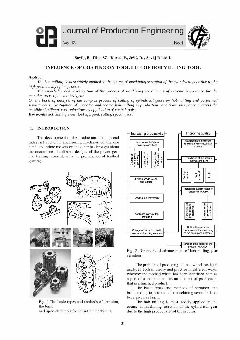
31
Sovilj, B. ,Tiba, SZ. ,Kovač, P., Ješić, D. , Sovilj-Nikić, I.
INFLUENCE OF COATING ON TOOL LIFE OF HOB MILLING TOOL Abstract
The hob milling is most widely applied in the course of machining serration of the cylindrical gear due to the high productivity of the process.
The knowledge and investigation of the process of machining serration is of extreme importance for the manufacturers of the toothed gear. On the basis of analysis of the complex process of cutting of cylindrical gears by hob milling and performed simultaneous investigation of uncoated and coated hob milling in production conditions, this paper presents the possible significant cost reductions by application of coated tools. Key words: hob milling wear, tool life, feed, cutting speed, gear. 1. INTRODUCTION
The development of the production tools, special
industrial and civil engineering machines on the one hand, and prime movers on the other has brought about the occurrence of different designs of the power gear and turning moment, with the prominence of toothed gearing.
Fig. 1.The basic types and methods of serration, the basic and up-to-date tools for serra-tion machining
Fig. 2. Directions of advancement of hob milling gear serration
The problem of producing toothed wheel has been analyzed both in theory and practice in different ways; whereby the toothed wheel has been identified both as a part of a machine and as an element of production, that is a finished product.
The basic types and methods of serration, the basic and up-to-date tools for machining serration have been given in Fig. 1.
The hob milling is most widely applied in the course of machining serration of the cylindrical gear due to the high productivity of the process.
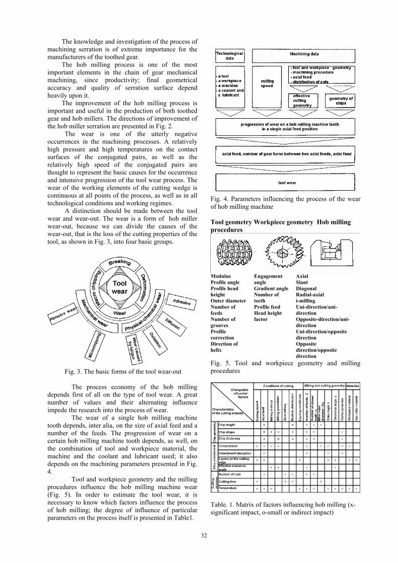
32
The knowledge and investigation of the process of machining serration is of extreme importance for the manufacturers of the toothed gear.
The hob milling process is one of the most important elements in the chain of gear mechanical machining, since productivity; final geometrical accuracy and quality of serration surface depend heavily upon it.
The improvement of the hob milling process is important and useful in the production of both toothed gear and hob millers. The directions of improvement of the hob miller serration are presented in Fig. 2.
The wear is one of the utterly negative occurrences in the machining processes. A relatively high pressure and high temperatures on the contact surfaces of the conjugated pairs, as well as the relatively high speed of the conjugated pairs are thought to represent the basic causes for the occurrence and intensive progression of the tool wear process. The wear of the working elements of the cutting wedge is continuous at all points of the process, as well as in all technological conditions and working regimes.
A distinction should be made between the tool wear and wear-out. The wear is a form of hob miller wear-out, because we can divide the causes of the wear-out, that is the loss of the cutting properties of the tool, as shown in Fig. 3, into four basic groups.
Fig. 3. The basic forms of the tool wear-out
The process economy of the hob milling depends first of all on the type of tool wear. A great number of values and their alternating influence impede the research into the process of wear.
The wear of a single hob milling machine tooth depends, inter alia, on the size of axial feed and a number of the feeds. The progression of wear on a certain hob milling machine tooth depends, as well, on the combination of tool and workpiece material, the machine and the coolant and lubricant used; it also depends on the machining parameters presented in Fig. 4.
Tool and workpiece geometry and the milling procedures influence the hob milling machine wear (Fig. 5). In order to estimate the tool wear, it is necessary to know which factors influence the process of hob milling; the degree of influence of particular parameters on the process itself is presented in Table1.
Fig. 4. Parameters influencing the process of the wear of hob milling machine
Tool geometry Workpiece geometry Hob milling procedures
Modulus Profile angle Profile head height Outer diameter Number of feeds Number of grooves Profile correction Direction of helix
Engagement angle Gradient angle Number of teeth Profile feed Head height factor
Axial Slant Diagonal Radial-axial i-milling Uni-direction/uni-direction Opposite-direction/uni-direction Uni-direction/opposite direction Opposite direction/opposite direction
Fig. 5. Tool and workpiece geometry and milling procedures
Table. 1. Matrix of factors influencing hob milling (x-significant impact, o-small or indirect impact)
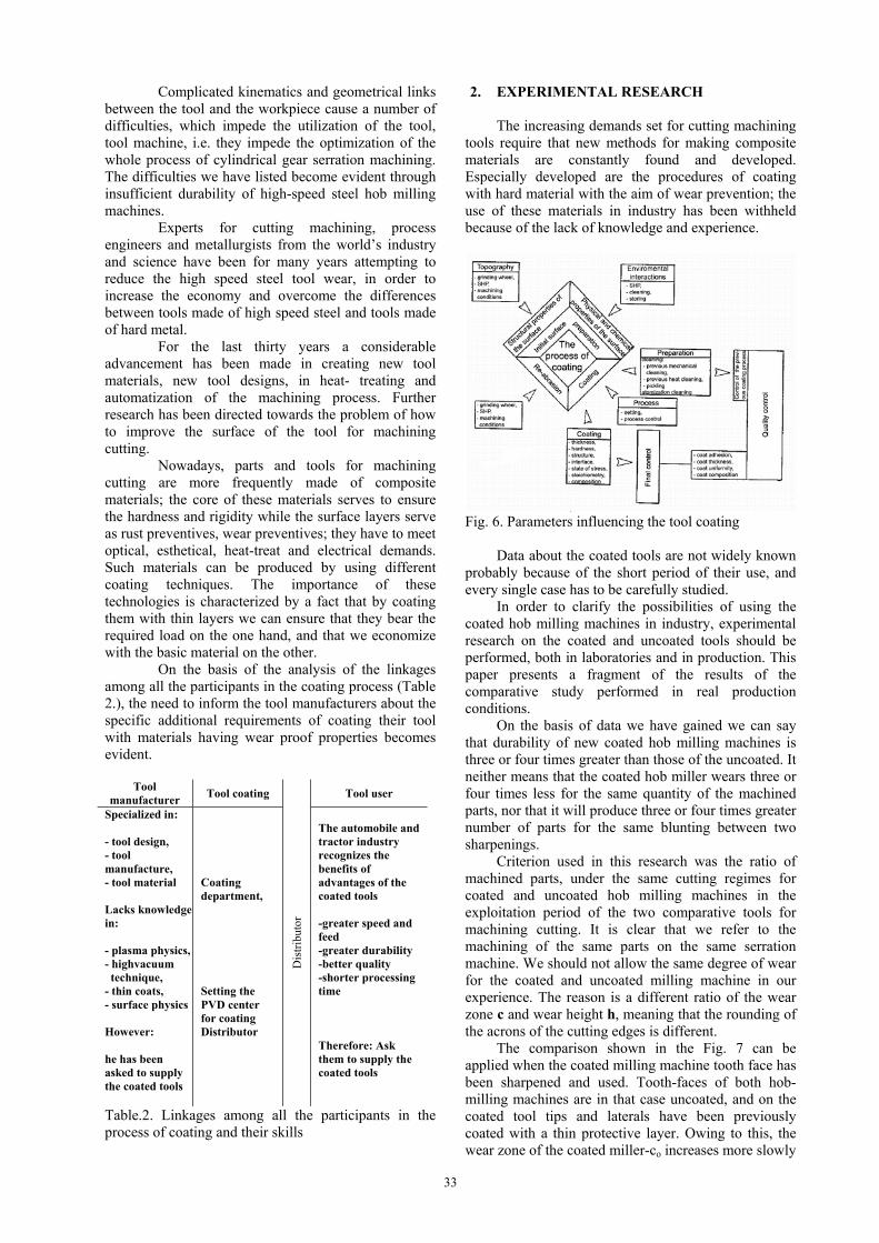
33
Complicated kinematics and geometrical links between the tool and the workpiece cause a number of difficulties, which impede the utilization of the tool, tool machine, i.e. they impede the optimization of the whole process of cylindrical gear serration machining. The difficulties we have listed become evident through insufficient durability of high-speed steel hob milling machines.
Experts for cutting machining, process engineers and metallurgists from the world’s industry and science have been for many years attempting to reduce the high speed steel tool wear, in order to increase the economy and overcome the differences between tools made of high speed steel and tools made of hard metal.
For the last thirty years a considerable advancement has been made in creating new tool materials, new tool designs, in heat- treating and automatization of the machining process. Further research has been directed towards the problem of how to improve the surface of the tool for machining cutting.
Nowadays, parts and tools for machining cutting are more frequently made of composite materials; the core of these materials serves to ensure the hardness and rigidity while the surface layers serve as rust preventives, wear preventives; they have to meet optical, esthetical, heat-treat and electrical demands. Such materials can be produced by using different coating techniques. The importance of these technologies is characterized by a fact that by coating them with thin layers we can ensure that they bear the required load on the one hand, and that we economize with the basic material on the other.
On the basis of the analysis of the linkages among all the participants in the coating process (Table 2.), the need to inform the tool manufacturers about the specific additional requirements of coating their tool with materials having wear proof properties becomes evident.
Tool manufacturer
Tool coating Tool user
Specialized in: - tool design, - tool manufacture, - tool material Lacks knowledge in: - plasma physics, - highvacuum technique, - thin coats, - surface physics However: he has been asked to supply the coated tools
Coating department, Setting the PVD center for coating Distributor
Dis
trib
utor
The automobile and tractor industry recognizes the benefits of advantages of the coated tools -greater speed and feed -greater durability -better quality -shorter processing time Therefore: Ask them to supply the coated tools
Table.2. Linkages among all the participants in the process of coating and their skills
2. EXPERIMENTAL RESEARCH
The increasing demands set for cutting machining tools require that new methods for making composite materials are constantly found and developed. Especially developed are the procedures of coating with hard material with the aim of wear prevention; the use of these materials in industry has been withheld because of the lack of knowledge and experience.
Fig. 6. Parameters influencing the tool coating
Data about the coated tools are not widely known
probably because of the short period of their use, and every single case has to be carefully studied.
In order to clarify the possibilities of using the coated hob milling machines in industry, experimental research on the coated and uncoated tools should be performed, both in laboratories and in production. This paper presents a fragment of the results of the comparative study performed in real production conditions.
On the basis of data we have gained we can say that durability of new coated hob milling machines is three or four times greater than those of the uncoated. It neither means that the coated hob miller wears three or four times less for the same quantity of the machined parts, nor that it will produce three or four times greater number of parts for the same blunting between two sharpenings.
Criterion used in this research was the ratio of machined parts, under the same cutting regimes for coated and uncoated hob milling machines in the exploitation period of the two comparative tools for machining cutting. It is clear that we refer to the machining of the same parts on the same serration machine. We should not allow the same degree of wear for the coated and uncoated milling machine in our experience. The reason is a different ratio of the wear zone c and wear height h, meaning that the rounding of the acrons of the cutting edges is different.
The comparison shown in the Fig. 7 can be applied when the coated milling machine tooth face has been sharpened and used. Tooth-faces of both hob-milling machines are in that case uncoated, and on the coated tool tips and laterals have been previously coated with a thin protective layer. Owing to this, the wear zone of the coated miller-co increases more slowly
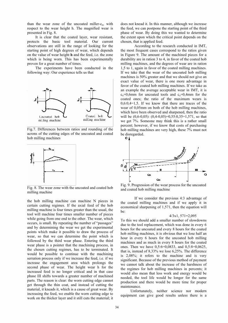
34
than the wear zone of the uncoated miller-cn, with respect to the wear height h. The magnified wear is presented in Fig. 8.
It is clear that the coated layer, wear resistant, protects the basic tool material. Our current observations are still in the range of looking for the starting point of high degrees of wear, which depends on the value of wear height h and the feed, i.e. the zone which is being worn. This has been experimentally proven for a great number of times.
The experiments have been conducted in the following way: Our experience tells us that
Fig.7. Differences between ratios and rounding of the acrons of the cutting edges of the uncoated and coated hob milling machines
Fig. 8. The wear zone with the uncoated and coated hob milling machine the hob milling machine can machine N pieces in certain cutting regimes. If the axial feed of the hob milling machine is four times greater than the usual, the tool will machine four times smaller number of pieces while going from one end to the other. The wear, which occurs, is small. By repeating the number of “passages” and by determining the wear we get the experimental points which make it possible to draw the process of wear, so that we can determine the point which is followed by the third wear phase. Entering the third wear phase is a pointer that the machining process, in the chosen cutting regimes, has to be terminated. It would be possible to continue with the machining serration process only if we increase the feed, i.e. if we increase the engagement area which prolongs the second phase of wear. The height wear h for the increased feed is no longer critical and in that case phase III shifts towards a greater number of machined parts. The reason is clear: the worn cutting edge cannot get through the thin coat, and instead of cutting the material, it kneads it, which is a cause of great wear. By increasing the feed, we enable the worn cutting edge to work on the thicker layer and it still cuts the material; it
does not knead it. In this manner, although we increase the feed, we can postpone the starting point of the third phase of wear. By doing this we wanted to determine the extent upon which the critical point depends on the chosen, that is applied feed.
According to the research conducted in IMT, the most frequent cases correspond to the ratios given in Figure 9. The amount of the machined pieces for a durability are in ration 3 to 4, in favor of the coated hob milling machines, and the degrees of wear are in ration 1,5 to 1, again in favor of the coated milling machines. If we take that the wear of the uncoated hob milling machines is 50% greater and that we should not give an exact value of wear, there is one more advantage in favor of the coated hob milling machines. If we take as an example the average acceptable wear in IMT, it is cn=0,6mm for uncoated tools and co=0,4mm for the coated ones; the ratio of the maximum wears is 0,6:0,4=1,5. If we know that there are traces of the wear of 0,05mm on both of the hob milling machines, which have been observed and sharpened, then the ratio will be (0,6-0,05): (0,4-0,05)=0,55:0,35=1,571, so that we get 7%. Someone may think this is a rather small percent; however, if we know that costs of purchasing hob milling machines are very high, these 7% must not be disregarded.
Fig. 9. Progression of the wear process for the uncoated and coated hob milling machine
If we consider the previous 4:3 advantage of the coated milling machines and if we apply it in economical sharpening of 1,571, then the equation will be: 4/3x1, 571=2,095 To this we should add a smaller number of slowdowns due to the tool replacement, which was done in every 6 hours for the uncoated and every 8 hours for the coated hob milling machines, it is obvious that we lose half an hour in every 6 hours for the uncoated hob milling machines and as much in every 8 hours for the coated ones. Then we have 0,5:6=0,0833, and 0,5:8=0,0625, that is, instead of 8,33% we lose 6,25%. The difference is 2,08%; it refers to the machine and is very significant. Because of the previous method of payment we cannot talk about the increase of the harshness of the regimes for hob milling machines in percents; it would also mean that less work and energy would be needed, the tool life would be longer for the same production and there would be more time for proper maintenance.
Unfortunately, neither science nor modern equipment can give good results unless there is a

35
proper use of hob milling machines and unless we get a proper feedback from the factories. 3. CONCLUSION
On the basis of the analysis of the complex
process of serration machining of the cylindrical gear by hob milling and conducted comparative investigation of the uncoated and coated hob milling machines in IMT, a conclusion has been reached that significant savings can be made by using the coated tools. The hob milling process is one of the most important elements in the chain of gear mechanical machining, since productivity, final accuracy and quality of the gear depend heavily upon it. One of the basic cutting parameters, which influences the machining time and process economy, is the feed. The increase of feed has a less significant influence upon the wear increase than the increase of cutting speed.
REFERENCES [1]. Barrov, G. : Wear of cutting tools,
Tribology, 5, No.1, 1972. [2]. Ivkovic, B. : Tribologija rezanja,
Gradjevinska knjiga, Beograd, 1979.
[3]. Kelly, W. D. : Gear cutting with TiN - coated tools, American machinist, 1982.
[4]. Sovilj, B. : Identifikacija triboloskih procesa pri odvalnom glodanju, Disertacija, Fakultet tehnickih nauka, Novi Sad, 1988.
[5]. Sovilj, B., Radonjić, S.,Sovilj-Nikić, I.: Analysis of application of profiled tools for seration in "Kolubara-Metal" factory, Journal of production Engineering, Volume number 12, No.1, pp.75-78, 2009.
[6]. Stanic, J. : Teorija obrade metala I, Masinski fakultet, Beograd, 1986.
Authors: Prof. dr Bogdan Sovilj, Prof. dr Pavel Kovač, Ivan Sovilj-Nikić,, Univerzitet u Novom Sadu,Fakultet tehničkih nauka, Trg Dositeja Obradovića 6,21000 Novi Sad, Srbija, FAX:+38121458133 ,TEL:+38121450366, D.Sc. Eng Zsolt TIBA,. University of Debrecen, Faculty of Technical Egineering, Department of Mechanical Engineering , Debrecen, Hungary, Dr Dušan Ješić, Tribotehnik, Rijeka, Croatia E-mail: [email protected]

36
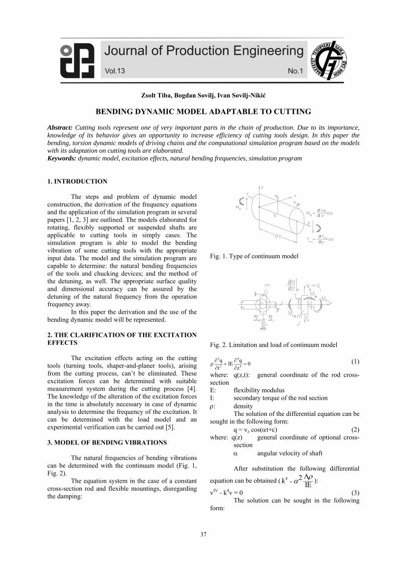
37
Zsolt Tiba, Bogdan Sovilj, Ivan Sovilj-Nikić
BENDING DYNAMIC MODEL ADAPTABLE TO CUTTING Abstract: Cutting tools represent one of very important parts in the chain of production. Due to its importance, knowledge of its behavior gives an opportunity to increase efficiency of cutting tools design. In this paper the bending, torsion dynamic models of driving chains and the computational simulation program based on the models with its adaptation on cutting tools are elaborated. Keywords: dynamic model, excitation effects, natural bending frequencies, simulation program 1. INTRODUCTION
The steps and problem of dynamic model construction, the derivation of the frequency equations and the application of the simulation program in several papers [1, 2, 3] are outlined. The models elaborated for rotating, flexibly supported or suspended shafts are applicable to cutting tools in simply cases. The simulation program is able to model the bending vibration of some cutting tools with the appropriate input data. The model and the simulation program are capable to determine: the natural bending frequencies of the tools and chucking devices; and the method of the detuning, as well. The appropriate surface quality and dimensional accuracy can be assured by the detuning of the natural frequency from the operation frequency away.
In this paper the derivation and the use of the bending dynamic model will be represented. 2. THE CLARIFICATION OF THE EXCITATION EFFECTS
The excitation effects acting on the cutting tools (turning tools, shaper-and-planer tools), arising from the cutting process, can’t be eliminated. These excitation forces can be determined with suitable measurement system during the cutting process [4]. The knowledge of the alteration of the excitation forces in the time is absolutely necessary in case of dynamic analysis to determine the frequency of the excitation. It can be determined with the load model and an experimental verification can be carried out [5]. 3. MODEL OF BENDING VIBRATIONS
The natural frequencies of bending vibrations can be determined with the continuum model (Fig. 1, Fig. 2).
The equation system in the case of a constant cross-section rod and flexible mountings, disregarding the damping:
Fig. 1. Type of continuum model
Fig. 2. Limitation and load of continuum model
2 4
2 4
q qIE 0
t z
(1)
where: q(z,t): general coordinate of the rod cross-section E: flexibility modulus I: secondary torque of the rod section : density
The solution of the differential equation can be sought in the following form:
q = vz cos(t+) (2) where: q(z) general coordinate of optional cross-
section angular velocity of shaft
After substitution the following differential
equation can be obtained ( k4 2 A
IE):
vIV - k4v = 0 (3) The solution can be sought in the following
form:
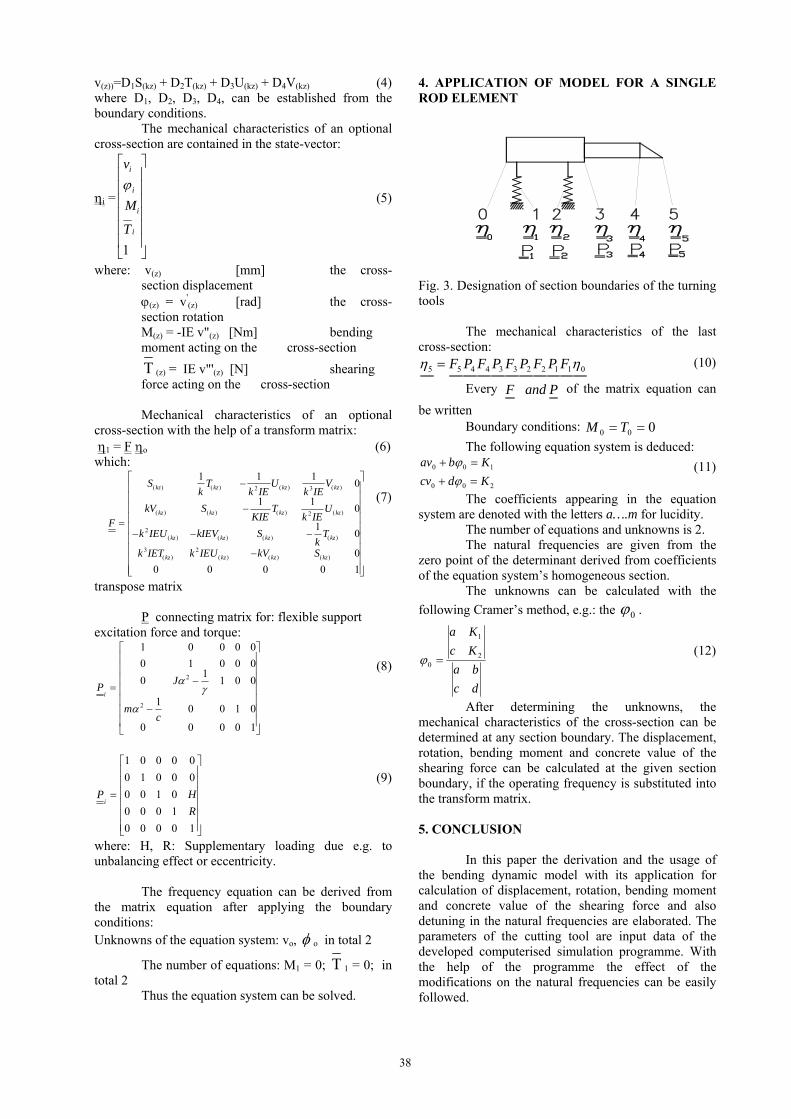
38
v(z))=D1S(kz) + D2T(kz) + D3U(kz) + D4V(kz) (4) where D1, D2, D3, D4, can be established from the boundary conditions.
The mechanical characteristics of an optional cross-section are contained in the state-vector:
i =
v
M
T
i
i
i
i
1
(5)
where: v(z) [mm] the cross-section displacement (z) = v'
(z) [rad] the cross-section rotation M(z) = -IE v"(z) [Nm] bending moment acting on the cross-section
T (z) = IE v"'(z) [N] shearing force acting on the cross-section
Mechanical characteristics of an optional
cross-section with the help of a transform matrix: 1 = F o (6)
which:
F
Sk
Tk IE
Uk IE
V
kV SKIE
Tk IE
U
k IEU kIEV Sk
T
k IET k IEU kV S
kz kz kz kz
kz kz kz kz
kz kz kz kz
kz kz kz kz
( ) ( ) ( ) ( )
( ) ( ) ( ) ( )
( ) ( ) ( ) ( )
( ) ( ) ( ) ( )
1 1 10
1 10
10
0
0 0 0 0 1
2 3
2
2
3 2
(7)
transpose matrix
P connecting matrix for: flexible support excitation force and torque:
PJ
mc
i
1 0 0 0 0
0 1 0 0 0
01
1 0 0
10 0 1 0
0 0 0 0 1
2
2
(8)
P H
Ri
1 0 0 0 0
0 1 0 0 0
0 0 1 0
0 0 0 1
0 0 0 0 1
(9)
where: H, R: Supplementary loading due e.g. to unbalancing effect or eccentricity.
The frequency equation can be derived from the matrix equation after applying the boundary conditions: Unknowns of the equation system: vo, o in total 2
The number of equations: M1 = 0; T 1 = 0; in total 2
Thus the equation system can be solved.
4. APPLICATION OF MODEL FOR A SINGLE ROD ELEMENT
Fig. 3. Designation of section boundaries of the turning tools
The mechanical characteristics of the last cross-section:
01122334455 FPFPFPFPF (10)
Every PandF of the matrix equation can
be written Boundary conditions: 000 TM
The following equation system is deduced:
200
100
Kdcv
Kbav
(11)
The coefficients appearing in the equation system are denoted with the letters a….m for lucidity.
The number of equations and unknowns is 2. The natural frequencies are given from the
zero point of the determinant derived from coefficients of the equation system’s homogeneous section.
The unknowns can be calculated with the
following Cramer’s method, e.g.: the 0 .
dc
ba
Kc
Ka
2
1
0 (12)
After determining the unknowns, the mechanical characteristics of the cross-section can be determined at any section boundary. The displacement, rotation, bending moment and concrete value of the shearing force can be calculated at the given section boundary, if the operating frequency is substituted into the transform matrix. 5. CONCLUSION
In this paper the derivation and the usage of the bending dynamic model with its application for calculation of displacement, rotation, bending moment and concrete value of the shearing force and also detuning in the natural frequencies are elaborated. The parameters of the cutting tool are input data of the developed computerised simulation programme. With the help of the programme the effect of the modifications on the natural frequencies can be easily followed.

39
6. REFERENCES [1] Tiba, ZS.: Bestimmung der Bewegungsgleichung von Kardanantrieben , DE MFK Tudományos Közlemények 2: pp.43-53. 2004 [2] Tiba, ZS.: Dynamische Modelle für die
Beschreibung der Torsions- und Biege-Schwingungen von Kardangetrieben. DE MFK Tudományos Közlemények 1:pp. 67-79.2005
[3] Tiba, ZS.,.: Dynamic behavior of long cardan drives used in agricultural machines Progress in Agricultural Engineering Sciences 2: pp. 1-35. .2006
[4] Varga G., Dudas, I., Csermely T.: Twist Drill Vibration at Environmentally Conscious Manufacturing, Proceedings of the 3rd Int. Conf. on Quality, Reliability, and aintenance, Oxford, United Kingdom, March 30-31, pp.: 383-386., 2000,
[5] Tiba, ZS.: Notwendigkeit der Modellbildung und Simulation bei der Dimensionerung mechanischer Konstrukcionen. DE MFK Tudományos Közlemények 1: 1, 2002
[6] Sovilj, B., Radonjić, S.,Sovilj-Nikić, I.: Analysis of application of profiled tools for seration in "Kolubara-Metal" factory, Journal of production Engineering, Volume number 12, No.1, pp.75-78, 2009.
Authors: D.Sc. Eng Zsolt Tiba,. University of Debrecen, Faculty of Technical Egineering, Department of Mechanical Engineering , Debrecen, Hungary, Prof. dr Bogdan Sovilj, Ivan Sovilj-Nikić,, Univerzitet u Novom Sadu,Fakultet tehničkih nauka, Trg Dositeja Obradovića 6,21000 Novi Sad, Srbija, FAX:+38121458133 ,TEL:+38121450366, E-mail: [email protected]

40
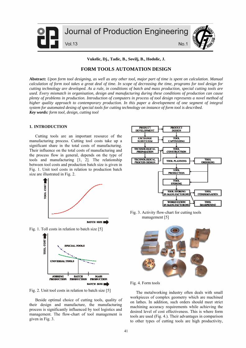
41
Vukelic, Dj., Tadic, B., Sovilj, B., Hodolic, J.
FORM TOOLS AUTOMATION DESIGN Abstract: Upon form tool designing, as well as any other tool, major part of time is spent on calculation. Manual calculation of form tool takes a great deal of time. In scope of decreasing the time, programs for tool design for cutting technology are developed. As a rule, in conditions of batch and mass production, special cutting tools are used. Every mismatch in organisation, design and manufacturing during these conditions of production can cause plenty of problems in production. Introduction of computers in process of tool design represents a novel method of higher quality approach to contemporary production. In this paper a developement of one segment of integral system for automated desing of special tools for cutting technology on instance of form tool is described. Key words: form tool, design, cutting tool 1. INTRODUCTION Cutting tools are an important resource of the manufacturing process. Cutting tool costs take up a significant share in the total costs of manufacturing. Their influence on the total costs of manufacturing and the process flow in general, depends on the type of tools and manufacturing [1, 2]. The relationship between tool costs and production batch size is given in Fig. 1. Unit tool costs in relation to production batch size are illustrated in Fig. 2.
Fig. 1. Toll costs in relation to batch size [5]
Fig. 2. Unit tool costs in relation to batch size [5] Beside optimal choice of cutting tools, quality of their design and manufacture, the manufacturing process is significantly influenced by tool logistics and management. The flow-chart of tool management is given in Fig. 3.
Fig. 3. Activity flow-chart for cutting tools
management [5]
Fig. 4. Form tools The metalworking industry often deals with small workpieces of complex geometry which are machined on lathes. In addition, such orders should meet strict machining accuracy requirements while achieving the desired level of cost effectiveness. This is where form tools are used (Fig. 4.). Their advantages in comparison to other types of cutting tools are high productivity,
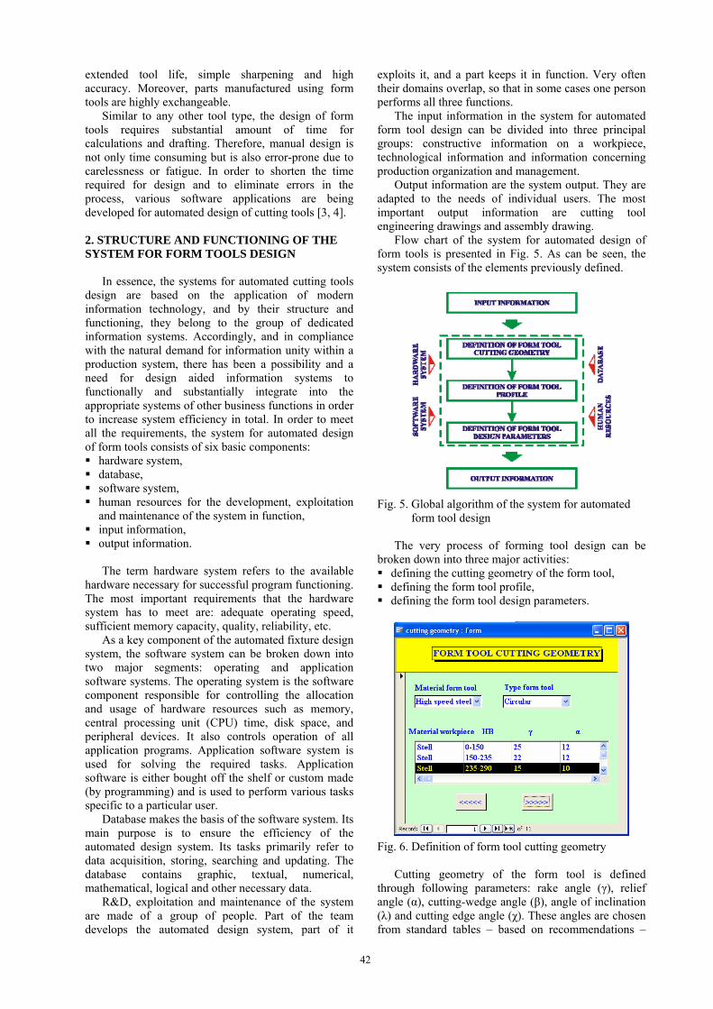
42
extended tool life, simple sharpening and high accuracy. Moreover, parts manufactured using form tools are highly exchangeable. Similar to any other tool type, the design of form tools requires substantial amount of time for calculations and drafting. Therefore, manual design is not only time consuming but is also error-prone due to carelessness or fatigue. In order to shorten the time required for design and to eliminate errors in the process, various software applications are being developed for automated design of cutting tools [3, 4]. 2. STRUCTURE AND FUNCTIONING OF THE SYSTEM FOR FORM TOOLS DESIGN In essence, the systems for automated cutting tools design are based on the application of modern information technology, and by their structure and functioning, they belong to the group of dedicated information systems. Accordingly, and in compliance with the natural demand for information unity within a production system, there has been a possibility and a need for design aided information systems to functionally and substantially integrate into the appropriate systems of other business functions in order to increase system efficiency in total. In order to meet all the requirements, the system for automated design of form tools consists of six basic components: hardware system, database, software system, human resources for the development, exploitation
and maintenance of the system in function, input information, output information. The term hardware system refers to the available hardware necessary for successful program functioning. The most important requirements that the hardware system has to meet are: adequate operating speed, sufficient memory capacity, quality, reliability, etc. As a key component of the automated fixture design system, the software system can be broken down into two major segments: operating and application software systems. The operating system is the software component responsible for controlling the allocation and usage of hardware resources such as memory, central processing unit (CPU) time, disk space, and peripheral devices. It also controls operation of all application programs. Application software system is used for solving the required tasks. Application software is either bought off the shelf or custom made (by programming) and is used to perform various tasks specific to a particular user. Database makes the basis of the software system. Its main purpose is to ensure the efficiency of the automated design system. Its tasks primarily refer to data acquisition, storing, searching and updating. The database contains graphic, textual, numerical, mathematical, logical and other necessary data. R&D, exploitation and maintenance of the system are made of a group of people. Part of the team develops the automated design system, part of it
exploits it, and a part keeps it in function. Very often their domains overlap, so that in some cases one person performs all three functions. The input information in the system for automated form tool design can be divided into three principal groups: constructive information on a workpiece, technological information and information concerning production organization and management. Output information are the system output. They are adapted to the needs of individual users. The most important output information are cutting tool engineering drawings and assembly drawing. Flow chart of the system for automated design of form tools is presented in Fig. 5. As can be seen, the system consists of the elements previously defined.
Fig. 5. Global algorithm of the system for automated
form tool design The very process of forming tool design can be broken down into three major activities: defining the cutting geometry of the form tool, defining the form tool profile, defining the form tool design parameters.
Fig. 6. Definition of form tool cutting geometry Cutting geometry of the form tool is defined through following parameters: rake angle (γ), relief angle (α), cutting-wedge angle (β), angle of inclination (λ) and cutting edge angle (χ). These angles are chosen from standard tables – based on recommendations –
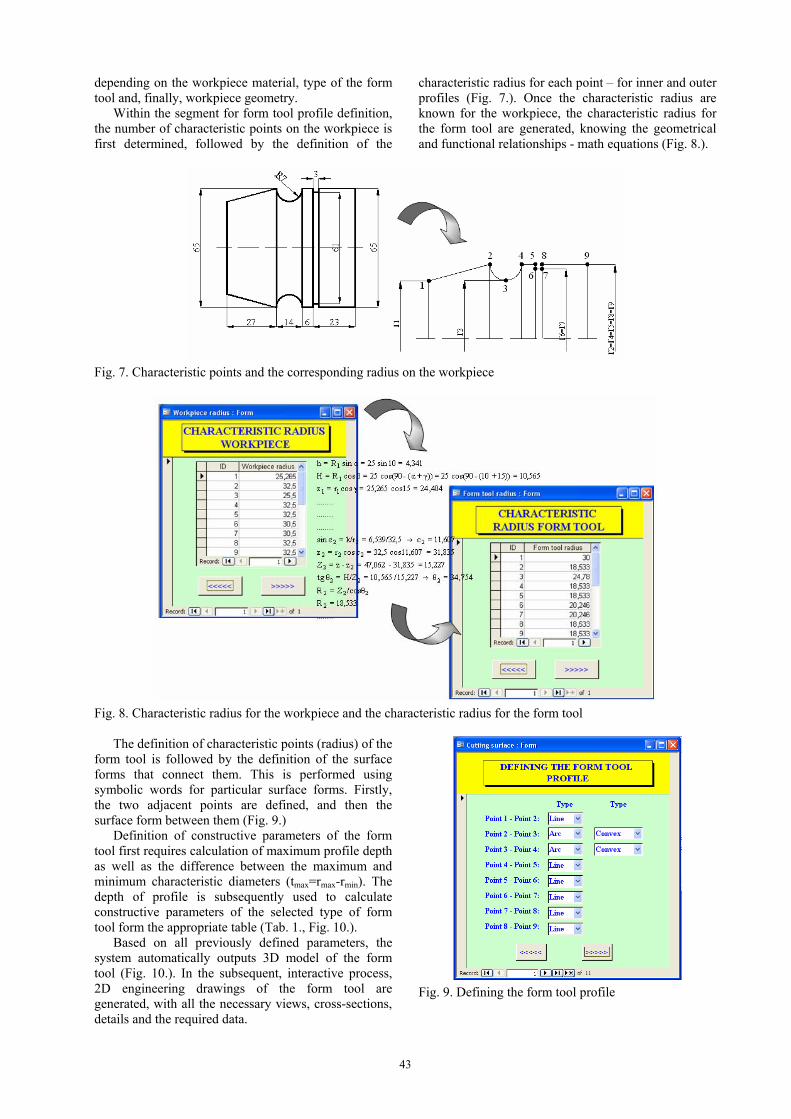
43
depending on the workpiece material, type of the form tool and, finally, workpiece geometry. Within the segment for form tool profile definition, the number of characteristic points on the workpiece is first determined, followed by the definition of the
characteristic radius for each point – for inner and outer profiles (Fig. 7.). Once the characteristic radius are known for the workpiece, the characteristic radius for the form tool are generated, knowing the geometrical and functional relationships - math equations (Fig. 8.).
Fig. 7. Characteristic points and the corresponding radius on the workpiece
Fig. 8. Characteristic radius for the workpiece and the characteristic radius for the form tool The definition of characteristic points (radius) of the form tool is followed by the definition of the surface forms that connect them. This is performed using symbolic words for particular surface forms. Firstly, the two adjacent points are defined, and then the surface form between them (Fig. 9.) Definition of constructive parameters of the form tool first requires calculation of maximum profile depth as well as the difference between the maximum and minimum characteristic diameters (tmax=rmax-rmin). The depth of profile is subsequently used to calculate constructive parameters of the selected type of form tool form the appropriate table (Tab. 1., Fig. 10.). Based on all previously defined parameters, the system automatically outputs 3D model of the form tool (Fig. 10.). In the subsequent, interactive process, 2D engineering drawings of the form tool are generated, with all the necessary views, cross-sections, details and the required data.
Fig. 9. Defining the form tool profile
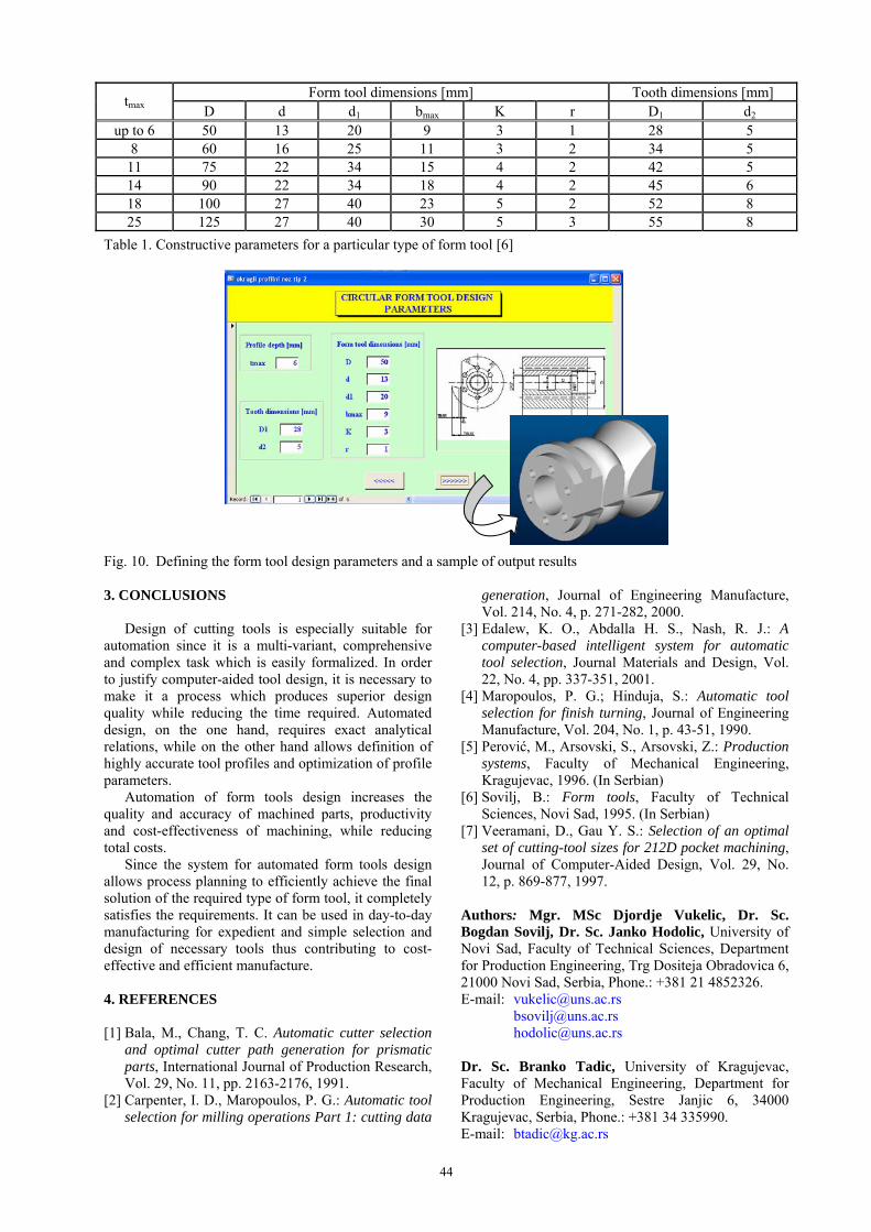
44
Form tool dimensions [mm] Tooth dimensions [mm] tmax D d d1 bmax K r D1 d2
up to 6 50 13 20 9 3 1 28 5 8 60 16 25 11 3 2 34 5
11 75 22 34 15 4 2 42 5 14 90 22 34 18 4 2 45 6 18 100 27 40 23 5 2 52 8 25 125 27 40 30 5 3 55 8
Table 1. Constructive parameters for a particular type of form tool [6]
Fig. 10. Defining the form tool design parameters and a sample of output results 3. CONCLUSIONS Design of cutting tools is especially suitable for automation since it is a multi-variant, comprehensive and complex task which is easily formalized. In order to justify computer-aided tool design, it is necessary to make it a process which produces superior design quality while reducing the time required. Automated design, on the one hand, requires exact analytical relations, while on the other hand allows definition of highly accurate tool profiles and optimization of profile parameters. Automation of form tools design increases the quality and accuracy of machined parts, productivity and cost-effectiveness of machining, while reducing total costs. Since the system for automated form tools design allows process planning to efficiently achieve the final solution of the required type of form tool, it completely satisfies the requirements. It can be used in day-to-day manufacturing for expedient and simple selection and design of necessary tools thus contributing to cost-effective and efficient manufacture. 4. REFERENCES [1] Bala, M., Chang, T. C. Automatic cutter selection
and optimal cutter path generation for prismatic parts, International Journal of Production Research, Vol. 29, No. 11, pp. 2163-2176, 1991.
[2] Carpenter, I. D., Maropoulos, P. G.: Automatic tool selection for milling operations Part 1: cutting data
generation, Journal of Engineering Manufacture, Vol. 214, No. 4, p. 271-282, 2000.
[3] Edalew, K. O., Abdalla H. S., Nash, R. J.: A computer-based intelligent system for automatic tool selection, Journal Materials and Design, Vol. 22, No. 4, pp. 337-351, 2001.
[4] Maropoulos, P. G.; Hinduja, S.: Automatic tool selection for finish turning, Journal of Engineering Manufacture, Vol. 204, No. 1, p. 43-51, 1990.
[5] Perović, M., Arsovski, S., Arsovski, Z.: Production systems, Faculty of Mechanical Engineering, Kragujevac, 1996. (In Serbian)
[6] Sovilj, B.: Form tools, Faculty of Теchnical Sciences, Novi Sad, 1995. (In Serbian)
[7] Veeramani, D., Gau Y. S.: Selection of an optimal set of cutting-tool sizes for 212D pocket machining, Journal of Computer-Aided Design, Vol. 29, No. 12, p. 869-877, 1997.
Authors: Mgr. MSc Djordje Vukelic, Dr. Sc. Bogdan Sovilj, Dr. Sc. Janko Hodolic, University of Novi Sad, Faculty of Technical Sciences, Department for Production Engineering, Trg Dositeja Obradovica 6, 21000 Novi Sad, Serbia, Phone.: +381 21 4852326. E-mail: [email protected] [email protected] [email protected] Dr. Sc. Branko Tadic, University of Kragujevac, Faculty of Mechanical Engineering, Department for Production Engineering, Sestre Janjic 6, 34000 Kragujevac, Serbia, Phone.: +381 34 335990. E-mail: [email protected]
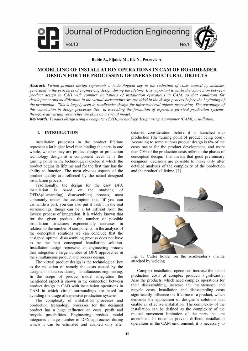
45
Babic A., Pljakic M., Ilic N., Petrovic A.
MODELLING OF INSTALLATION OPERATIONS IN CAM OF ROADHEADER DESIGN FOR THE PROCESSING OF INFRASTRUCTURAL OBJECTS
Abstract: Virtual product design represents a technological key to the reduction of costs caused by mistakes generated in the processes of engineering design during the lifetime. It is important to make the connection between product design in CAD with complex limitations of installation operations in CAM, so that conditions for development and modification in the virtual surroundins are provided in the design process before the beginning of the production. This is largely seen in roadheader design for infrastructural objects processing. The advantage of this connection in design processes lies in exceeding the formation of expensive physical production systems, therefore all variant researches are done on a virtual model. Key words: Product design using a computer (CAD), technology design using a computer (CAM), installation..
1. INTRODUCTION
Installation processes in the product lifetime represent a lot higher level than binding the parts in one whole, whether they are product design or production technology design at a component level. It is the turning point in the technological cycles at which the product begins its lifetime and for the first time has the ability to function. The most obvious aspects of the product quality are reflected by the actual designed installation process.
Traditionally, the design for the easy DFA installation is based on the studying of DFDA(dismantling) disassembling process, most commonly under the assumption that ’if you can dismantle a part, you can also put it back’. In the real surroundings, things can be a lot diffrent from the inverse process of integration. It is widely known that for the given product, the number of possible installation structures exponentially increases in relation to the number of components. In the analysis of the conceptual solutions we can conclude that the designed optimal disassembling process does not have to be the best conceptual installation solution. Installation design represents an engineering process that integrates a large number of DFX approaches in the simultaneous product and process design.
The virtual product design is the technological key to the reduction of namely the costs caused by the designers’ mistakes during simultaneous engineering. In the scope of product model integration the mentioned aspect is shown in the connection between product design in CAD with installation operations in CAM in which virtual surroundings are based on avoiding the usage of expensive production systems.
The complexity of installation processes and production technology processes for the designed product has a huge influence on costs, profit and recycle possibilities. Engineering product model integrates a large number of DFX approaches during which it can be estimated and adapted only after
detailed consideration before it is launched into production (the turning point of product being born). According to some authors product design is 6% of the costs meant for the product development, and more than 70% of the production costs refers to the phases of conceptual design. That means that good preliminary designers’ decisions are possible to make only after detailed analyses of the complexity of the production and the product’s lifetime. [1]
Fig. 1. Cutter holder on the roadheader’s mantle attached by welding
Complex installation operations increase the actual production costs of complex products significantly. Also the products, which need complex operations for their disassembling, increase the maintenance and recycle costs. Installation and disassembling costs significantly influence the lifetime of a product, which demands the application of designer’s solutions that enable an effective installation. The complexity of the installation can be defined as the complexity of the mutual movement limitation of the parts that are assembled. In order to prevent difficult installation operations in the CAM environment, it is necessary to
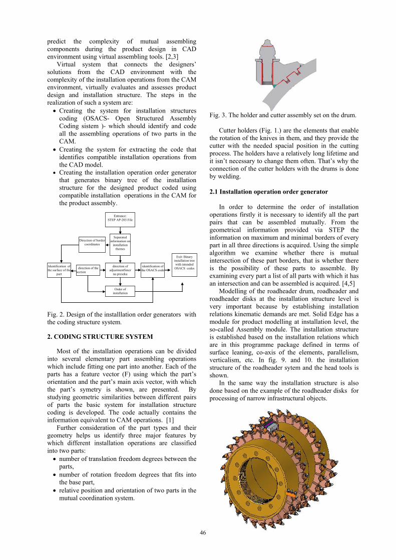
46
predict the complexity of mutual assembling components during the product design in CAD environment using virtual assembling tools. [2,3]
Virtual system that connects the designers’ solutions from the CAD environment with the complexity of the installation operations from the CAM environment, virtually evaluates and assesses product design and installation structure. The steps in the realization of such a system are: Creating the system for installation structures
coding (OSACS- Open Structured Assembly Coding sistem )- which should identify and code all the assembling operations of two parts in the CAM.
Creating the system for extracting the code that identifies compatible installation operations from the CAD model.
Creating the installation operation order generator that generates binary tree of the installation structure for the designed product coded using compatible installation operations in the CAM for the product assembly.
Fig. 2. Design of the installlation order generators with the coding structure system. 2. CODING STRUCTURE SYSTEM
Most of the installation operations can be divided into several elementary part assembling operations which include fitting one part into another. Each of the parts has a feature vector (F) using which the part’s orientation and the part’s main axis vector, with which the part’s symetry is shown, are presented. By studying geometric similarities between different pairs of parts the basic system for installation structure coding is developed. The code actually contains the information equivalent to CAM operations. [1]
Further consideration of the part types and their geometry helps us identify three major features by which different installation operations are classified into two parts: number of translation freedom degrees between the
parts, number of rotation freedom degrees that fits into
the base part, relative position and orientation of two parts in the
mutual coordination system.
Fig. 3. The holder and cutter assembly set on the drum.
Cutter holders (Fig. 1.) are the elements that enable
the rotation of the knives in them, and they provide the cutter with the needed spacial position in the cutting process. The holders have a relatively long lifetime and it isn’t necessary to change them often. That’s why the connection of the cutter holders with the drums is done by welding. 2.1 Installation operation order generator
In order to determine the order of installation operations firstly it is necessary to identify all the part pairs that can be assembled mutually. From the geometrical information provided via STEP the information on maximum and minimal borders of every part in all three directions is acquired. Using the simple algorithm we examine whether there is mutual intersection of these part borders, that is whether there is the possibility of these parts to assemble. By examining every part a list of all parts with which it has an intersection and can be assembled is acquired. [4,5]
Modelling of the roadheader drum, roadheader and roadheader disks at the installation structure level is very important because by establishing installation relations kinematic demands are met. Solid Edge has a module for product modelling at installation level, the so-called Assembly module. The installation structure is established based on the installation relations which are in this programme package defined in terms of surface leaning, co-axis of the elements, parallelism, verticalism, etc. In fig. 9. and 10. the installation structure of the roadheader sytem and the head tools is shown.
In the same way the installation structure is also done based on the example of the roadheader disks for processing of narrow infrastructural objects.
Exit: Binary installation tree with intended
OSACS codes
Entrance: STEP AP-203 File
Separated information on
installation themes
Direction of border coordinates
direction of adjustmentSmer
na preseku
identification of the OSACS code
Order of installation
direction of the section
Identification of the surface of the
part
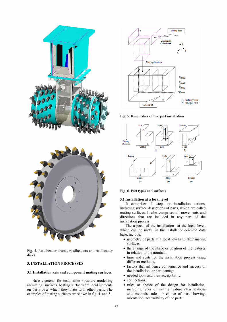
47
Fig. 4. Roadheader drums, roadheaders and roadheader disks 3. INSTALLATION PROCESSES 3.1 Installation axis and component mating surfaces
Base elements for installation structure modelling
aremating surfaces. Mating surfaces are local elements on parts over which they mate with other parts. The examples of mating surfaces are shown in fig. 4. and 5.
Fig. 5. Kinematics of two part installation
Fig. 6. Part types and surfaces 3.2 Installation at a local level
It comprises all steps or installation actions, including surface desriptions of parts, which are called mating surfaces. It also comprises all movements and directions that are included in any part of the installation process
The aspects of the installation at the local level, which can be useful in the installation-oriented data base, include: geometry of parts at a local level and their mating
surfaces, the change of the shape or position of the features
in relation to the nominal, time and costs for the installation process using
different methods, factors that influence convenience and success of
the installation, or part damage, needed tools and their accessibility, connections, rules or choice of the design for installation,
including types of mating feature classifications and methods, rules or choice of part showing, orientation, accessibility of the parts.
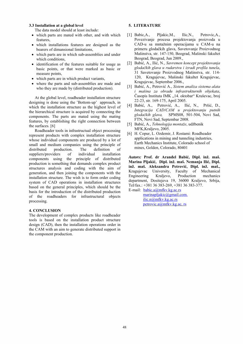
48
3.3 Installation at a global level The data model should at least include:
which parts are mated with other, and with which features,
which installations features are designed as the bearers of dimansional limitations,
which parts are in which sub-assemblies and under which conditions,
identification of the features suitable for usage as basic points, or that were marked as basic or measure points,
which parts are in which product variants, where the parts and sub-assemblies are made and
who they are made by (distributed production).
At the global level, roadheader installation structure designing is done using the ’Bottom-up’ approach, in which the installation structure as the highest level of the hierarchical structure is acquired by connecting the components. The parts are mated using the mating features, by establishing the right connection between the surfaces. [6]
Roadheader tools in infrastructual object processing represent products with complex installation structure whose individual components are produced by a lot of small and medium companies using the principle of distributed production. The definition of suppliers/providers of individual installation components using the principle of distributed production is something that demands complex product structures analysis and coding with the aim of generation, and then joining the components with the installation structure. The wish is to form order coding system of CAD operations in installation structures based on the general principles, which should be the basis for the introduction of the distributed production of the roadheaders for infrastructural objects processing.
4. CONCLUSION The development of complex products like roadheader tools is based on the installation product structure design (CAD), then the installation operations order in the CAM with an aim to generate distributed support in the component production.
5. LITERATURE
[1] Babic,A., Pljakic,M., Ilic,N., Petrovic,A., Povezivanje procesa projektovanja proizvoda u CAD-u sa mntažnim operacijama u CAM-u na primeru glodačkih glava, Savetovanje Proizvodnog Mašinstva, str. 147-150, Beograd, Mašinski fakultet Beograd, Beograd, Jun 2009.,
[2] Babić, A., Ilić, N., Savremen koncept projektovanja glodačkih glava u rudarstvu i izradi profila tunela, 31 Savetovanje Proizvodnog Mašinstva, str. 114-120, Kragujevac, Mašinski fakultet Kragujevac, Kragujevac, Septembar 2006.,
[3] Babić, A., Petrović A., Sistem analiza sistema alata i mašina za obradu infrastrukturnih objekata, Časopis Instituta IMK „14. oktobar“ Kruševac, broj 22-23, str. 169-175, April 2005.
[4] Babić, A., Petrović, A., Ilić, N., Pršić, D., Integracija CAD/CAM u projektovanju putnih glodačkih glava, SPMS08, 501-504, Novi Sad, FTN, Novi Sad, Septembar 2008.
[5] Babić, A., Tehnologija montaže, udžbenik MFK,Kraljevo, 2005.
[6] H. Copur, L. Ozdemir, J. Rostami: Roadheader applications in mining and tunneling industries, Earth Mechanics Institute, Colorado school of mines, Golden, Colorado, 80401
Autors: Prof. dr Aranđel Babić, Dipl. inž. maš. Marina Pljakić, Dipl. inž. maš. Nemanja Ilić, Dipl. inž. maš. Aleksandra Petrović, Dipl. inž. maš., Kragujevac University, Faculty of Mechanical Engineering Kraljevo, Production mechanics department, Dositejeva 19, 36000 Kraljevo, Srbija, Tel/fax.: +381 36 383-269, +381 36 383-377. E-mail: [email protected]
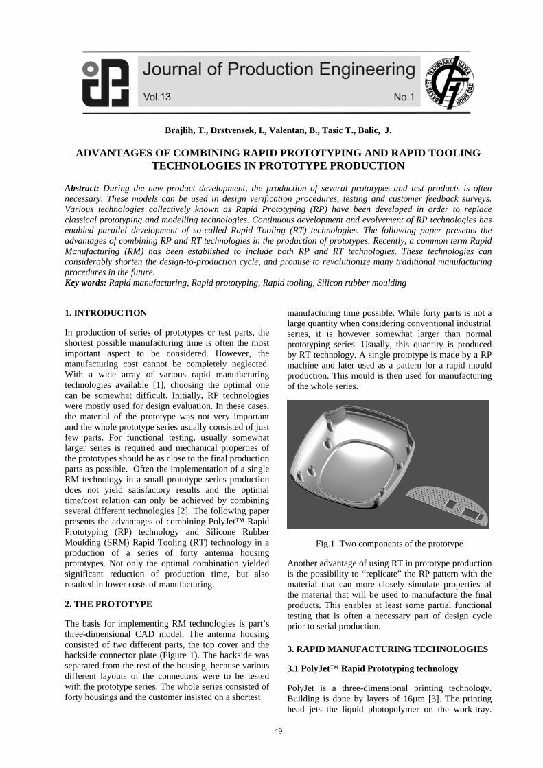
49
Brajlih, T., Drstvensek, I., Valentan, B., Tasic T., Balic, J.
ADVANTAGES OF COMBINING RAPID PROTOTYPING AND RAPID TOOLING TECHNOLOGIES IN PROTOTYPE PRODUCTION
Abstract: During the new product development, the production of several prototypes and test products is often necessary. These models can be used in design verification procedures, testing and customer feedback surveys. Various technologies collectively known as Rapid Prototyping (RP) have been developed in order to replace classical prototyping and modelling technologies. Continuous development and evolvement of RP technologies has enabled parallel development of so-called Rapid Tooling (RT) technologies. The following paper presents the advantages of combining RP and RT technologies in the production of prototypes. Recently, a common term Rapid Manufacturing (RM) has been established to include both RP and RT technologies. These technologies can considerably shorten the design-to-production cycle, and promise to revolutionize many traditional manufacturing procedures in the future. Key words: Rapid manufacturing, Rapid prototyping, Rapid tooling, Silicon rubber moulding
1. INTRODUCTION
In production of series of prototypes or test parts, the shortest possible manufacturing time is often the most important aspect to be considered. However, the manufacturing cost cannot be completely neglected. With a wide array of various rapid manufacturing technologies available [1], choosing the optimal one can be somewhat difficult. Initially, RP technologies were mostly used for design evaluation. In these cases, the material of the prototype was not very important and the whole prototype series usually consisted of just few parts. For functional testing, usually somewhat larger series is required and mechanical properties of the prototypes should be as close to the final production parts as possible. Often the implementation of a single RM technology in a small prototype series production does not yield satisfactory results and the optimal time/cost relation can only be achieved by combining several different technologies [2]. The following paper presents the advantages of combining PolyJet™ Rapid Prototyping (RP) technology and Silicone Rubber Moulding (SRM) Rapid Tooling (RT) technology in a production of a series of forty antenna housing prototypes. Not only the optimal combination yielded significant reduction of production time, but also resulted in lower costs of manufacturing.
2. THE PROTOTYPE
The basis for implementing RM technologies is part’s three-dimensional CAD model. The antenna housing consisted of two different parts, the top cover and the backside connector plate (Figure 1). The backside was separated from the rest of the housing, because various different layouts of the connectors were to be tested with the prototype series. The whole series consisted of forty housings and the customer insisted on a shortest
manufacturing time possible. While forty parts is not a large quantity when considering conventional industrial series, it is however somewhat larger than normal prototyping series. Usually, this quantity is produced by RT technology. A single prototype is made by a RP machine and later used as a pattern for a rapid mould production. This mould is then used for manufacturing of the whole series.
Fig.1. Two components of the prototype
Another advantage of using RT in prototype production is the possibility to “replicate” the RP pattern with the material that can more closely simulate properties of the material that will be used to manufacture the final products. This enables at least some partial functional testing that is often a necessary part of design cycle prior to serial production. 3. RAPID MANUFACTURING TECHNOLOGIES
3.1 PolyJet™ Rapid Prototyping technology
PolyJet is a three-dimensional printing technology. Building is done by layers of 16µm [3]. The printing head jets the liquid photopolymer on the work-tray.
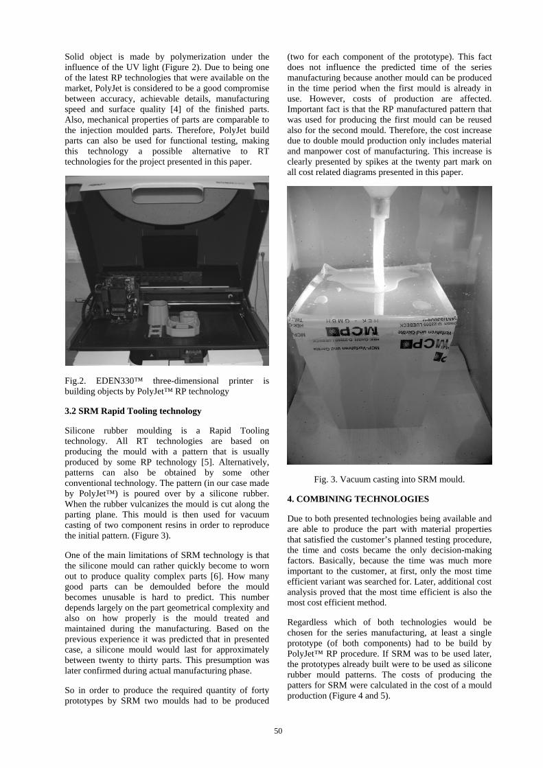
50
Solid object is made by polymerization under the influence of the UV light (Figure 2). Due to being one of the latest RP technologies that were available on the market, PolyJet is considered to be a good compromise between accuracy, achievable details, manufacturing speed and surface quality [4] of the finished parts. Also, mechanical properties of parts are comparable to the injection moulded parts. Therefore, PolyJet build parts can also be used for functional testing, making this technology a possible alternative to RT technologies for the project presented in this paper.
Fig.2. EDEN330™ three-dimensional printer is building objects by PolyJet™ RP technology
3.2 SRM Rapid Tooling technology
Silicone rubber moulding is a Rapid Tooling technology. All RT technologies are based on producing the mould with a pattern that is usually produced by some RP technology [5]. Alternatively, patterns can also be obtained by some other conventional technology. The pattern (in our case made by PolyJet™) is poured over by a silicone rubber. When the rubber vulcanizes the mould is cut along the parting plane. This mould is then used for vacuum casting of two component resins in order to reproduce the initial pattern. (Figure 3).
One of the main limitations of SRM technology is that the silicone mould can rather quickly become to worn out to produce quality complex parts [6]. How many good parts can be demoulded before the mould becomes unusable is hard to predict. This number depends largely on the part geometrical complexity and also on how properly is the mould treated and maintained during the manufacturing. Based on the previous experience it was predicted that in presented case, a silicone mould would last for approximately between twenty to thirty parts. This presumption was later confirmed during actual manufacturing phase.
So in order to produce the required quantity of forty prototypes by SRM two moulds had to be produced
(two for each component of the prototype). This fact does not influence the predicted time of the series manufacturing because another mould can be produced in the time period when the first mould is already in use. However, costs of production are affected. Important fact is that the RP manufactured pattern that was used for producing the first mould can be reused also for the second mould. Therefore, the cost increase due to double mould production only includes material and manpower cost of manufacturing. This increase is clearly presented by spikes at the twenty part mark on all cost related diagrams presented in this paper.
Fig. 3. Vacuum casting into SRM mould.
4. COMBINING TECHNOLOGIES
Due to both presented technologies being available and are able to produce the part with material properties that satisfied the customer’s planned testing procedure, the time and costs became the only decision-making factors. Basically, because the time was much more important to the customer, at first, only the most time efficient variant was searched for. Later, additional cost analysis proved that the most time efficient is also the most cost efficient method.
Regardless which of both technologies would be chosen for the series manufacturing, at least a single prototype (of both components) had to be build by PolyJet™ RP procedure. If SRM was to be used later, the prototypes already built were to be used as silicone rubber mould patterns. The costs of producing the patters for SRM were calculated in the cost of a mould production (Figure 4 and 5).
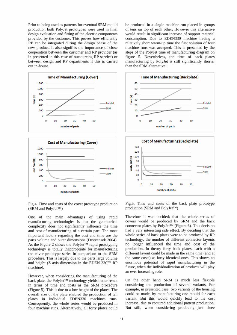
51
Prior to being used as patterns for eventual SRM mould production both PolyJet prototypes were used in final design evaluation and fitting of the electric components provided by the customer. This proves how efficiently RP can be integrated during the design phase of the new product. It also signifies the importance of close cooperation between the customer and RP provider (as in presented in this case of outsourcing RP service) or between design and RP departments if this is carried out in-house.
Fig.4. Time and costs of the cover prototype production (SRM and PolyJet™)
One of the main advantages of using rapid manufacturing technologies is that the geometrical complexity does not significantly influence the time and cost of manufacturing of a certain part. The most important factors regarding the cost and time are the parts volume and outer dimensions (Drstvensek 2004). As the Figure 2 shows the PolyJet™ rapid prototyping technology is totally inappropriate for manufacturing the cover prototype series in comparison to the SRM procedure. This is largely due to the parts large volume and height (Z axis dimension in the EDEN 330™ RP machine).
However, when considering the manufacturing of the back plate, the PolyJet™ technology yields better result in terms of time and costs as the SRM procedure (Figure 5). This is due to a low height of the plates. The overall size of the plate enabled the production of ten plates in individual EDEN330 machines runs. Consequently, the whole series would be produced in four machine runs. Alternatively, all forty plates could
be produced in a single machine run placed in groups of tens on top of each other. However this alternative would result in significant increase of support material consumption. Due to EDEN330 machine having a relatively short warm-up time the first solution of four machine runs was accepted. This is presented by the steps of the PolyJet time of manufacturing diagram on figure 5. Nevertheless, the time of back plates manufacturing by PolyJet is still significantly shorter than the SRM alternative.
Fig.5. Time and costs of the back plate prototype production (SRM and PolyJet™)
Therefore it was decided; that the whole series of covers would be produced by SRM and the back connector plates by PolyJet™ (Figure 6). This decision had a very interesting side effect. By deciding that the whole series of back plates were to be produced by RP technology, the number of different connector layouts no longer influenced the time and cost of the production. In theory forty back plates, each with a different layout could be made in the same time (and at the same costs) as forty identical ones. This shows an enormous potential of rapid manufacturing in the future, when the individualization of products will play an ever increasing role.
On the other hand SRM is much less flexible considering the production of several variants. For example, in presented case, two variants of the housing could be made, by manufacturing one mould for each variant. But this would quickly lead to the cost increase, due to required additional pattern production. But still, when considering producing just three
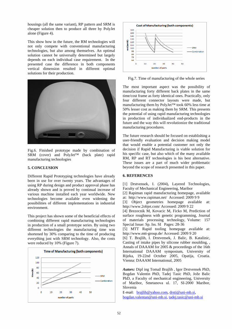
52
housings (all the same variant), RP pattern and SRM is cheaper solution then to produce all three by PolyJet alone (Figure 4).
This show how in the future, the RM technologies will not only compete with conventional manufacturing technologies, but also among themselves. An optimal solution cannot be universally determined but largely depends on each individual case requirement. In the presented case the difference in both components vertical dimension resulted in different optimal solutions for their production.
Fig.6. Finished prototype made by combination of SRM (cover) and PolyJet™ (back plate) rapid manufacturing technologies
5. CONCLUSION
Different Rapid Prototyping technologies have already been in use for over twenty years. The advantages of using RP during design and product approval phase has already shown and is proved by continual increase of various machine installed each year worldwide. New technologies become available even widening the possibilities of different implementations in industrial environment.
This project has shown some of the beneficial effects of combining different rapid manufacturing technologies in production of a small prototype series. By using two different technologies the manufacturing time was shortened by 30% comparing to the time of producing everything just with SRM technology. Also, the costs were reduced by 10% (Figure 7).
Fig.7. Time of manufacturing of the whole series
The most important aspect was the possibility of manufacturing forty different back plates in the same time/cost frame as forty identical ones. Practically, only four different connector layouts were made, but manufacturing them by PolyJet™ took 60% less time at 50% lesser cost as making them by SRM. This presents the potential of using rapid manufacturing technologies in production of individualized end-products in the future and the way this will revolutionize the traditional manufacturing procedures.
The future research should be focused on establishing a user-friendly evaluation and decision making model that would enable a potential customer not only the decision if Rapid Manufacturing is viable solution for his specific case, but also which of the many available RM, RP and RT technologies is his best alternative. These issues are a part of much wider problematic beyond the scope of research presented in this paper.
6. REFERENCES
[1] Drstvensek, I. (2004), Layered Technologies, Faculty of Mechanical Engineering, Maribor [2] Rapiman rapid manufacturing homepage, available at: http://www.rapiman.net/ Accessed: 2009 9 9 [3] Object geometries homepage available at: http://www.2objet.com/ Accessed: 2009 9 22 [4] Brezocnik M, Kovacic M, Ficko M, Prediction of surface roughness with genetic programming, Journal of materials processing technology, Volume: 157 Special Issue: Sp. Iss. SI Pages: 28-36 [5] MTT Rapid tooling homepage available at: http://www.mtt-group.de/ Accessed: 2009 9 20 [6] T. Brajlih, I. Drstvensek, J. Balic, B. Katalinic, Casting of intake pipes by silicone rubber moulding, , Annals of DAAAM for 2005 & proceedings of the 16th International DAAAM symposium, University of Rijeka, 19-22nd October 2005, Opatija, Croatia. Vienna: DAAAM International, 2005 Autors: Dipl ing Tomaž Brajlih , Igor Drstvensek PhD, Bogdan Valentin PhD, Tadej Tasic PhD, Jože Balic PhD, a Faculty of mechanical engineering, University of Maribor, Smetanova ul. 17, SI-2000 Maribor, Slovenia E‐mail: [email protected], [email protected], [email protected], [email protected]

53
Budak, I., Sokovic, M., Hodolic, J., Kopac, J. POINT DATA REDUCTION BASED ON FUZZY LOGICIN REVERSE ENGINEERING Abstract: Contemporary 3D-digitization systems for Reverse Engineering modelling are characterized by increased scanning speed and also by the possibility to generate large number of points in a short time. Generally, this improves the efficiency of the RE-modelling process. In practice however, a large number of points in the stage of generation of the CAD model may become a serious problem. Therefore, lately considerable attention is focused to the problem of point data reduction in the 3D-digitization results. This paper presents an approach for point data reduction based on fuzzy logic, along with the results of its practical application. Key words: Reverse Engineering, 3D-digitization, Point data reduction 1. INTRODUCTION Contemporary 3D-digitization systems which are applied in Reverse Engineering (RE) modelling are characterized by increased scanning speed and also by the possibility to generate large number of points in a short time. Generally, this improves the quality and efficiency of the RE-modelling process. In practice however, later in the stage of CAD model generation, a huge number of points which are generated in the stage of 3D-digitization may become a serious problem [1,2]. Considering all the above mentioned, the stage of pre-processing the results of 3D-digitization which includes error filtering, data smoothing and the most sophisticated process of data-point reduction, becomes inevitable in almost any RE system [3,4]. In the multitude of data-point reduction approaches that were developed, it is possible to identify three dominating groups of approaches for pre-processing the results of 3D-digitization: methods of point sampling, methods of polygon reduction and grid methods [5, 6]. It should be noted that there are frequent attempts to integrate the methods of artificial intelligence into the process of pre-processing, i.e. into point data reduction above all, in order to achieve better quality and process efficiency [1]. Within the framework of this article, a novel approach for point data reduction is introduced, designated primarily for RE modelling systems based on the "cross-sectional" approach. 2. THE NOVEL APPROACH FOR POINT DATA
REDUCTION
The main features of an approach for point data reduction presented here are integrated deviation analysis and fuzzy logic reasoning. This constitutes the main difference in comparison to the approaches developed so far.
Building on the weak spots and deficiencies of current approaches to reduction of point data by sampling methods - i.e. the lack of information on the level of deviation in reduced point clouds and necessity
to employ parameters which are abstract to user [4,5] - a novel approach was developed for analysis of the level of deviation of the reduced point cloud in comparison with the initial point cloud. This novel approach introduces an additional parameter termed maximum allowed reduction error (MARE), in the reduction-related decision process with the sampling-based methods.
In order to improve the process of reduction, the novel approach was enhanced by implementing fuzzy logic in the process of reduction-related decision making. Beside the additional improvement of the deviation/mean level of reduction ratio, implementation fuzzy logic allowed a more user-friendly and intuitive application. The reduction process is controlled by simply entering the deviation tolerance, allowing the user to gain better insight into the quality of the reduced point cloud [6,7]. The key feature of the novel approach to sampling-based point data reduction, proposed here, is the procedure for analysis of deviations of cross-sectional curves, which are the result of point data reduction.
Practical realization of procedure for analysis of deviation is based on computation and analysis of maximum deviation of the resulting cross-sectional curve relative to the original cross-sectional curve generated from initial point cloud. Least squares method, modified to meet specific requirements of the problem in hand, was used to compute maximum deviation - designated MRE (Maximum Reduction Error) in this paper. In this case, the key parameter of MRE is the absolute value of maximum deviation of a cubic spline curve generated through an array of scanned and reduced points - relative to the spline curve generated through original point array. In other words, MRE is computed after each point elimination by finding maximum deviation i(xi, yi) of the spline curve generated after elimination of j-th point Tj(xj, yj, zj) - relative to the spline curve generated through originally scanned point cloud (Fig. 1).
niMRE i ,...,2,1;)(max . (1)
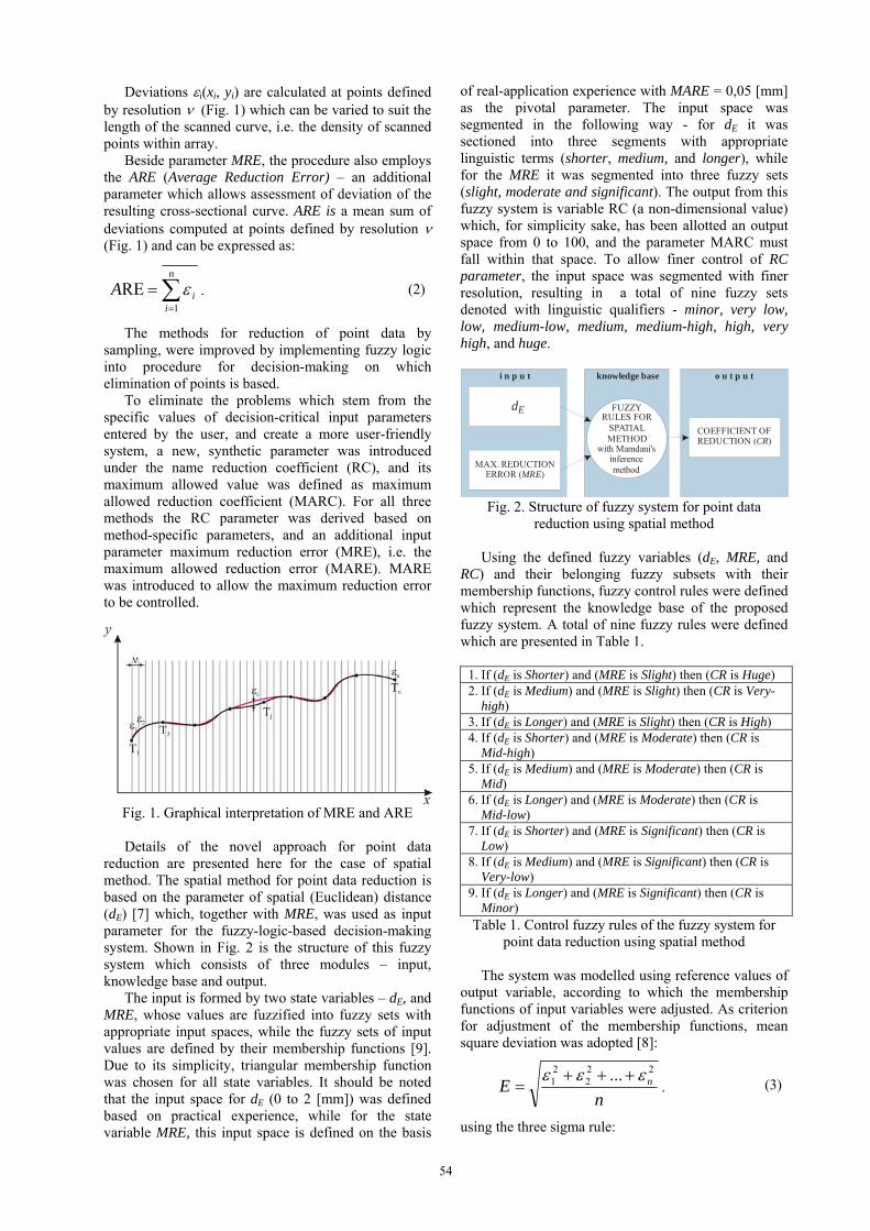
54
Deviations i(xi, yi) are calculated at points defined by resolution (Fig. 1) which can be varied to suit the length of the scanned curve, i.e. the density of scanned points within array.
Beside parameter MRE, the procedure also employs the ARE (Average Reduction Error) – an additional parameter which allows assessment of deviation of the resulting cross-sectional curve. ARE is a mean sum of deviations computed at points defined by resolution (Fig. 1) and can be expressed as:
n
iiA
1
RE . (2)
The methods for reduction of point data by sampling, were improved by implementing fuzzy logic into procedure for decision-making on which elimination of points is based.
To eliminate the problems which stem from the specific values of decision-critical input parameters entered by the user, and create a more user-friendly system, a new, synthetic parameter was introduced under the name reduction coefficient (RC), and its maximum allowed value was defined as maximum allowed reduction coefficient (MARC). For all three methods the RC parameter was derived based on method-specific parameters, and an additional input parameter maximum reduction error (MRE), i.e. the maximum allowed reduction error (MARE). MARE was introduced to allow the maximum reduction error to be controlled.
Fig. 1. Graphical interpretation of MRE and ARE
Details of the novel approach for point data
reduction are presented here for the case of spatial method. The spatial method for point data reduction is based on the parameter of spatial (Euclidean) distance (dE) [7] which, together with MRE, was used as input parameter for the fuzzy-logic-based decision-making system. Shown in Fig. 2 is the structure of this fuzzy system which consists of three modules – input, knowledge base and output.
The input is formed by two state variables – dE, and MRE, whose values are fuzzified into fuzzy sets with appropriate input spaces, while the fuzzy sets of input values are defined by their membership functions [9]. Due to its simplicity, triangular membership function was chosen for all state variables. It should be noted that the input space for dE (0 to 2 [mm]) was defined based on practical experience, while for the state variable MRE, this input space is defined on the basis
of real-application experience with MARE = 0,05 [mm] as the pivotal parameter. The input space was segmented in the following way - for dE it was sectioned into three segments with appropriate linguistic terms (shorter, medium, and longer), while for the MRE it was segmented into three fuzzy sets (slight, moderate and significant). The output from this fuzzy system is variable RC (a non-dimensional value) which, for simplicity sake, has been allotted an output space from 0 to 100, and the parameter MARC must fall within that space. To allow finer control of RC parameter, the input space was segmented with finer resolution, resulting in a total of nine fuzzy sets denoted with linguistic qualifiers - minor, very low, low, medium-low, medium, medium-high, high, very high, and huge.
MAX. REDUCTIONERROR ( )MRE
FUZZYRULES FOR
SPATIALMETHOD
with Mamdani'sinferencemethod
COEFFICIENT OFREDUCTION ( )CR
i n p u t knowledge base o u t p u t
dE
Fig. 2. Structure of fuzzy system for point data reduction using spatial method
Using the defined fuzzy variables (dE, MRE, and
RC) and their belonging fuzzy subsets with their membership functions, fuzzy control rules were defined which represent the knowledge base of the proposed fuzzy system. A total of nine fuzzy rules were defined which are presented in Table 1.
1. If (dE is Shorter) and (MRE is Slight) then (CR is Huge) 2. If (dE is Medium) and (MRE is Slight) then (CR is Very-
high) 3. If (dE is Longer) and (MRE is Slight) then (CR is High) 4. If (dE is Shorter) and (MRE is Moderate) then (CR is
Mid-high) 5. If (dE is Medium) and (MRE is Moderate) then (CR is
Mid) 6. If (dE is Longer) and (MRE is Moderate) then (CR is
Mid-low) 7. If (dE is Shorter) and (MRE is Significant) then (CR is
Low) 8. If (dE is Medium) and (MRE is Significant) then (CR is
Very-low) 9. If (dE is Longer) and (MRE is Significant) then (CR is
Minor) Table 1. Control fuzzy rules of the fuzzy system for
point data reduction using spatial method
The system was modelled using reference values of output variable, according to which the membership functions of input variables were adjusted. As criterion for adjustment of the membership functions, mean square deviation was adopted [8]:
nE n
222
21 ...
. (3)
using the three sigma rule:
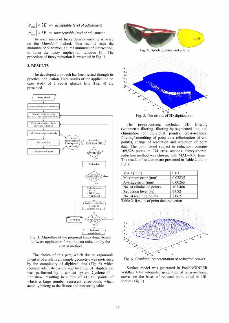
55
E3max => acceptable level of adjustment
E3max => unacceptable level of adjustment
The mechanism of fuzzy decision-making is based on the Mamdani method. This method uses the minimum of operation, i.e. the minimum of intersection, to form the fuzzy implication function [9]. The procedure of fuzzy reduction is presented in Fig. 3.
3. RESULTS
The developed approach has been tested through its practical application. Here results of the application on case study of a sports glasses lens (Fig. 4) are presented.
Scanned curve selectionk = 1,2,..., ; cross-sections no.n n=
Point set selection of thcurve for reduction
i-
Pre-reduction
Calculation of MRE
Fuzzycontrol rules
for spatialmethod
ReductionCoefficient (RC)
Reduction
Yes
No
Last point
c ?within scanned
urve
Calculations of[%]
[mm]
:- - -
RL MRE ARE [mm]
Reduced point dataof the th
scanned curve -i
Lastscanned curve
( = ) k n ?
Reducedpoint cloud
Recording
Cross-sectional data extraction
Point cloud
No
Yes
Calculation of parameter d
RC<MARC
Yes
No
E
Fig. 3. Algorithm of the proposed fuzzy-logic-based software application for point data reduction by the
spatial method
The choice of this part, which due to ergonomic intent is of a relatively simple geometry, was motivated by the complexity of digitized data (Fig. 5) which requires adequate fixture and locating. 3D digitization was performed by a contact system Cyclone II - Renishaw, resulting in a total of 412,111 points, of which a large number represent error-points which actually belong to the fixture and measuring table.
Fig. 4: Sports glasses and a lens
Fig. 5. The results of 3D-digitization
The pre-processing included 3D filtering
(volumetric filtering, filtering by segmented line, and elimination of individual points), cross-sectional filtering/smoothing of point data (elimination of end points), change of resolution and reduction of point data. The point cloud subject to reduction, contains 109,528 points in 214 cross-sections. Fuzzy-chordal reduction method was chosen, with MAD=0.03 [mm]. The results of reduction are presented in Table 2 and in Fig. 6.
MAD [mm] 0.03 Maximum error [mm] 0.02835 Average error [mm] 0.00265 No. of eliminated points 107,466 Reduction level [%] 97.82 No. of resulting points 2,062
Table 2. Results of point data reduction
Fig. 6. Graphical representation of reduction results
Surface model was generated in Pro/ENGINEER
Wildfire 4 by automated generation of cross-sectional curves on the bases of reduced point cloud in IBL format (Fig. 7).
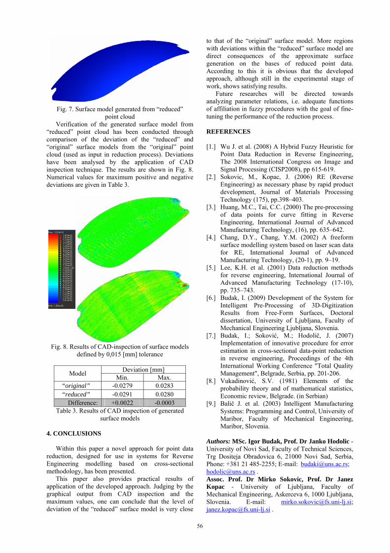
56
Fig. 7. Surface model generated from “reduced”
point cloud Verification of the generated surface model from
“reduced” point cloud has been conducted through comparison of the deviation of the “reduced” and “original” surface models from the “original” point cloud (used as input in reduction process). Deviations have been analysed by the application of CAD inspection technique. The results are shown in Fig. 8. Numerical values for maximum positive and negative deviations are given in Table 3.
Fig. 8. Results of CAD-inspection of surface models
defined by 0,015 [mm] tolerance Deviation [mm]
Model Min. Max.
“original” -0.0279 0.0283 “reduced” -0.0291 0.0280
Difference: +0.0022 -0.0003 Table 3. Results of CAD inspection of generated
surface models
4. CONCLUSIONS
Within this paper a novel approach for point data reduction, designed for use in systems for Reverse Engineering modelling based on cross-sectional methodology, has been presented.
This paper also provides practical results of application of the developed approach. Judging by the graphical output from CAD inspection and the maximum values, one can conclude that the level of deviation of the “reduced” surface model is very close
to that of the “original” surface model. More regions with deviations within the “reduced” surface model are direct consequences of the approximate surface generation on the bases of reduced point data. According to this it is obvious that the developed approach, although still in the experimental stage of work, shows satisfying results.
Future researches will be directed towards analyzing parameter relations, i.e. adequate functions of affiliation in fuzzy procedures with the goal of fine-tuning the performance of the reduction process. REFERENCES [1.] Wu J. et al. (2008) A Hybrid Fuzzy Heuristic for
Point Data Reduction in Reverse Engineering, The 2008 International Congress on Image and Signal Processing (CISP2008), pp 615-619.
[2.] Sokovic, M., Kopac, J. (2006) RE (Reverse Engineering) as necessary phase by rapid product development, Journal of Materials Processing Technology (175), pp.398–403.
[3.] Huang, M.C., Tai, C.C. (2000) The pre-processing of data points for curve fitting in Reverse Engineering, International Journal of Advanced Manufacturing Technology, (16), pp. 635–642.
[4.] Chang, D.Y., Chang, Y.M. (2002) A freeform surface modelling system based on laser scan data for RE, International Journal of Advanced Manufacturing Technology, (20-1), pp. 9–19.
[5.] Lee, K.H. et al. (2001) Data reduction methods for reverse engineering, International Journal of Advanced Manufacturing Technology (17-10), pp. 735–743.
[6.] Budak, I. (2009) Development of the System for Intelligent Pre-Processing of 3D-Digitization Results from Free-Form Surfaces, Doctoral dissertation, University of Ljubljana, Faculty of Mechanical Engineering Ljubljana, Slovenia.
[7.] Budak, I.; Soković, M.; Hodolič, J. (2007) Implementation of innovative procedure for error estimation in cross-sectional data-point reduction in reverse engineering, Proceedings of the 4th International Working Conference "Total Quality Management", Belgrade, Serbia, pp. 201-206.
[8.] Vukadinović, S.V. (1981) Elements of the probability theory and of mathematical statistics, Economic review, Belgrade. (in Serbian)
[9.] Balič J. et al. (2003) Intelligent Manufacturing Systems: Programming and Control, University of Maribor, Faculty of Mechanical Engineering, Maribor, Slovenia.
Authors: MSc. Igor Budak, Prof. Dr Janko Hodolic - University of Novi Sad, Faculty of Technical Sciences, Trg Dositeja Obradovica 6, 21000 Novi Sad, Serbia, Phone: +381 21 485-2255; E-mail: [email protected]; [email protected] . Assoc. Prof. Dr Mirko Sokovic, Prof. Dr Janez Kopac - University of Ljubljana, Faculty of Mechanical Engineering, Askerceva 6, 1000 Ljubljana, Slovenia. E-mail: [email protected]; [email protected] .
57
Luzanin, O., Vilotic, D., Movrin, D.
CAM SIMULATION FOR MANUFACTURE OF FORGING DIES FOR CAR WHEEL HUB – A CASE STUDY
Abstract: In the metalworking industries of the most industrially developed countries forging remains one of the dominating technologies. In order to achieve optimal performance throughout the various phases of design process, computer aided technologies must be applied extensively. Special importance is placed upon CAM simulations as an important aid in optimization of process planning. This paper is focused on application of CAM simulations as the final stage of a wider optimization process conducted in order to rationalize and enhance the conventional process of wheel hub manufacture. Key words: CAD/CAM, forging, dies, tool path simulation, 1. INTRODUCTION
Metal forming is the oldest metal processing technology. Its primitive origins can be dated back to prehistoric people who learned to smith virgin gold peaces and later to beat a heated sponge iron with a stone in order to form useful tools [1]. Despite its ancient origins and long tradition, forging continues to be at the forefront of modern manufacturing technologies in the developed countries. For example, according to Japan Forging Association the forging industry in Japan shall remain one of the leading industrial branches oriented towards manufacture of complex-geometry, high-precision, and high-quality parts. Moreover, in Europe exist approximately 1.000 companies which utilize forging technologies to manufacture parts from steel, aluminum, titanium and other alloys [2] . Optimal performance throughout the various phases of design process requires extensive application of computer aided technologies. Special importance is placed upon CAM simulations as an important aid in optimization of process planning.
Present-day CAD/CAM tools have reached maturity, enabling scientists and engineers to simulate manufacturing processes of various complexity. According to data from 2005, Forging reports that 80% of the large companies (more than 250 employees), 75% of the mid-sized companies (100-249), and even 50% of smaller firms (50-99) in the US are using CAM and process simulation tools [3]. These numbers have more than doubled over the last decade, similar to the expanded use of CAD systems during the 1980s.
This paper is focused on a study case of a CAM simulation for manufacture of a wheel hub, which was realized at the Laboratory for Technology of Plasticity, the Department for Production Engineering, Novi Sad. 2. BENEFITS FROM USING CAD/CAM TOOLS
Manufacturing parts using modern technology requires a typical engineering department to use three basic software programs:
the CAD software to make the design of the part the CAM software to calculate the tool paths
based on the design, compensating for the cutter's geometry, adding feedrate and spindle commands, etc.
the control software to read the tool paths and allow the machine tool to perform required motions and operations
Speaking of CAM software, since the early eighties of the 20th century, there have been developed a number of software tools specialized in technologies of forging. By providing detailed insight into the forging process prior to tool selection and important process decisions, forging simulation offers substantial cost and time savings. It allows simulation of a number of essential factors such as material flow, stresses and strains, temperatures, etc. It can also allow early detection of defects such as laps and under-fill of die cavities, thus enabling user to correct the mistakes before the production process is initiated.
Generally speaking, utilization of CAD/CAM software in forging helps to reduce [4],[5]:
number of die physical prototypes number of defects scrap and material waste number of shop floor trials product development time For the same reason, those software tools efficiently contribute to increase of:
product quality die life reliability flexibility process know-how.
58
Worth noting is the fact that on today’s CAM market, high-end software solutions have advanced features which include following [6]:
support for a fourth axis, or for full 5 axis machining
optimization for high speed machining (constant tool load)
special sequences for approaching and leaving the geometry (lead-ins)
automatic stepover calculation a wide choice of machining strategies, like
parallel, spiral, radial, pencil tracing, flat surface
recognition, offset machining, plunge milling and automatic smoothing of almost vertical surfaces.
automatic detection and removal of rest material management of undercuts rendered machining simulations. One such solution, NX CAM, is licensed to the Laboratory for Technology of Plasticity of the Department for Production Engineering in Novi Sad, and it is being used to generate process plans and NC part programs for manufacture of forging and other forming tools. 3. BASIC FEATURES OF NX-CAM MODULE
In general, NX is a complex Computer-Aided
Design, Computer-Aided Manufacturing, and Computer-Aided Engineering (CAD/CAM/CAE) system. The CAD functions automate the normal engineering, design, and drafting capabilities found in today's manufacturing companies, the CAM functions provide NC programming for modern machine tools using the NX design model to describe the finished part. The CAE functions provide a number of product, assembly, and part performance simulation abilities, across a broad range of engineering disciplines [6].
NX CAM – Integrated Simulation and Verification (ISV) is a part of NX system that allows the NC programmer to perform tool path and machine motion validation through digital simulation without leaving the programming session. The software is structured in a modular fashion and enables users to simulate tool path and material removal through complete machine tool motion simulation.
Using advanced simulation technology, full 3D in-process representations of the part, coupled with gouge and collision checking methods, ISV eliminates the need to utilize expensive production equipment to verify manufacturability. This system is completely integrated with NX CAM, which allows simulation process to be simultaneous with programming and provides immediate, real-time feedback and validation. Among numerous advantages offered to scientists and engineers, this systems allows following:
Verification of material removal and simulation of entire machine tool motion
Operates in NX CAM, within the NC programming session
Simultaneous collision detection and gouge checking
Accurate representation of machine tool kinematics and configuration
Modular software from metal removal verification to full machine tool simulation and the addition of new machines.
The system uses common Parasolid platform to
transfer geometry and other data across. Starting with the prepared CAD data of the part that has to be machined, the link with NX CAM is associative, which means that the link to original data is maintained through all stages of the process. 4. MOTIVATION BEHIND THE CASE STUDY The CAM simulation discussed in this paper represents the final stage of a multi-part optimization of a wheel hub manufacture by forging, conducted at the Laboratory for Technology of Plasticity.
The wheel hob for which this simulation was performed (Fig. 1) is a standard car part which is manufactured in large batches. The material of this part is Č1633 (C 53).
Fig. 1 Photo of car wheel hub In the stages precedent to this final stage, an exhaustive two-variant computer simulation was conducted in order to optimize the conventional forging process. One of the principal problems which was successfully eliminated through this simulation was insufficient mould filling. After the first optimization stage was completed, the moulds for the lower and upper part of the forging tool were designed in CAD, and the digital models were used as input for the second stage, where the CAM simulation was performed in order to generate the required NC programs for manufacture of moulds on a milling machine. 5. STAGES AND ACTIVITIES IN CREATION
OF CAM SIMULATION CAM simulation for the manufacture of wheel hob was conducted in several characteristic stages, which involved following:
1. Creation of the basic setup, which included specification of blank geometry, workpiece geometry, and clamping. Basic workpiece geometry
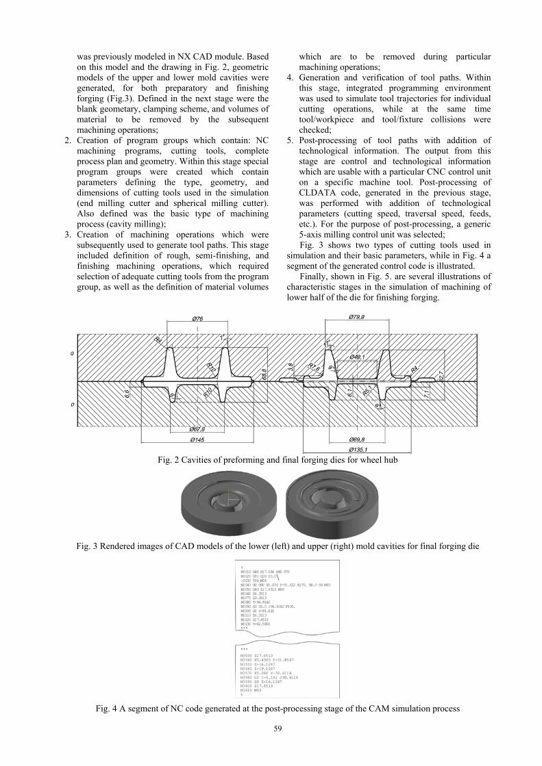
59
was previously modeled in NX CAD module. Based on this model and the drawing in Fig. 2, geometric models of the upper and lower mold cavities were generated, for both preparatory and finishing forging (Fig.3). Defined in the next stage were the blank geometary, clamping scheme, and volumes of material to be removed by the subsequent machining operations;
2. Creation of program groups which contain: NC machining programs, cutting tools, complete process plan and geometry. Within this stage special program groups were created which contain parameters defining the type, geometry, and dimensions of cutting tools used in the simulation (end milling cutter and spherical milling cutter). Also defined was the basic type of machining process (cavity milling);
3. Creation of machining operations which were subsequently used to generate tool paths. This stage included definition of rough, semi-finishing, and finishing machining operations, which required selection of adequate cutting tools from the program group, as well as the definition of material volumes
which are to be removed during particular machining operations;
4. Generation and verification of tool paths. Within this stage, integrated programming environment was used to simulate tool trajectories for individual cutting operations, while at the same time tool/workpiece and tool/fixture collisions were checked;
5. Post-processing of tool paths with addition of technological information. The output from this stage are control and technological information which are usable with a particular CNC control unit on a specific machine tool. Post-processing of CLDATA code, generated in the previous stage, was performed with addition of technological parameters (cutting speed, traversal speed, feeds, etc.). For the purpose of post-processing, a generic 5-axis milling control unit was selected; Fig. 3 shows two types of cutting tools used in
simulation and their basic parameters, while in Fig. 4 a segment of the generated control code is illustrated.
Finally, shown in Fig. 5. are several illustrations of characteristic stages in the simulation of machining of lower half of the die for finishing forging.
Fig. 2 Cavities of preforming and final forging dies for wheel hub
Fig. 3 Rendered images of CAD models of the lower (left) and upper (right) mold cavities for final forging die
\
Fig. 4 A segment of NC code generated at the post-processing stage of the CAM simulation process
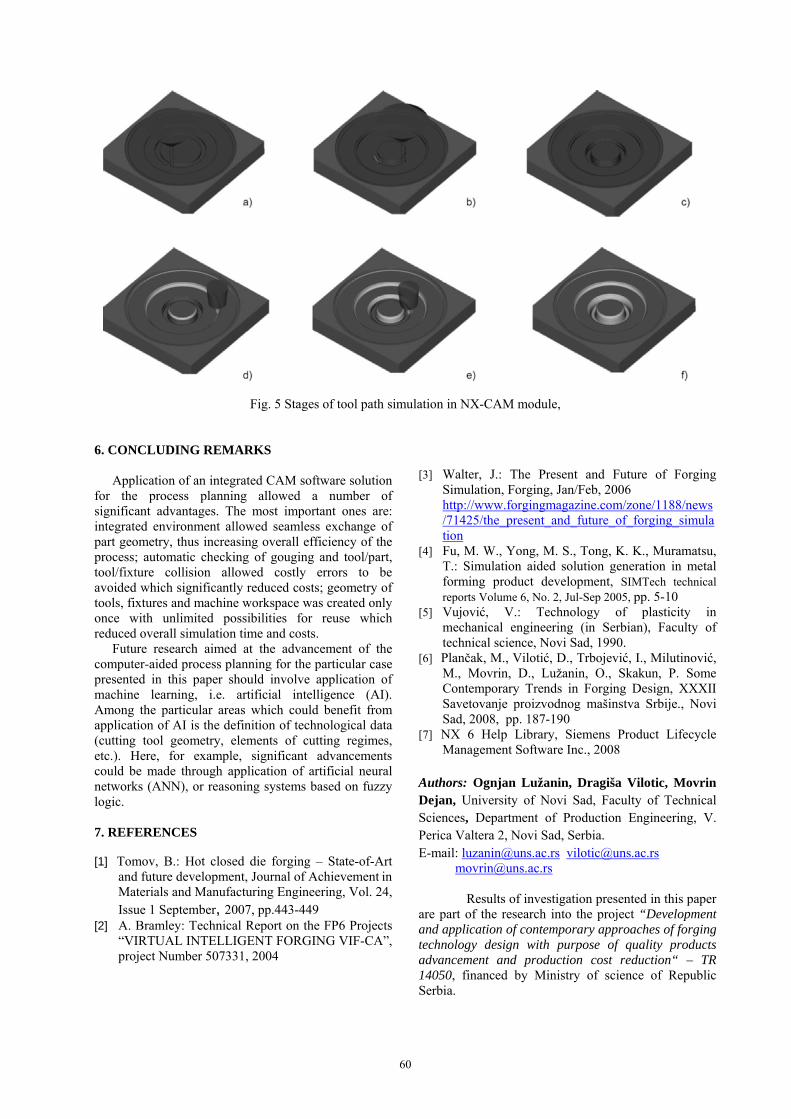
60
Fig. 5 Stages of tool path simulation in NX-CAM module, 6. CONCLUDING REMARKS Application of an integrated CAM software solution for the process planning allowed a number of significant advantages. The most important ones are: integrated environment allowed seamless exchange of part geometry, thus increasing overall efficiency of the process; automatic checking of gouging and tool/part, tool/fixture collision allowed costly errors to be avoided which significantly reduced costs; geometry of tools, fixtures and machine workspace was created only once with unlimited possibilities for reuse which reduced overall simulation time and costs. Future research aimed at the advancement of the computer-aided process planning for the particular case presented in this paper should involve application of machine learning, i.e. artificial intelligence (AI). Among the particular areas which could benefit from application of AI is the definition of technological data (cutting tool geometry, elements of cutting regimes, etc.). Here, for example, significant advancements could be made through application of artificial neural networks (ANN), or reasoning systems based on fuzzy logic. 7. REFERENCES [1] Tomov, B.: Hot closed die forging – State-of-Art
and future development, Journal of Achievement in Materials and Manufacturing Engineering, Vol. 24, Issue 1 September, 2007, pp.443-449
[2] A. Bramley: Technical Report on the FP6 Projects “VIRTUAL INTELLIGENT FORGING VIF-CA”, project Number 507331, 2004
[3] Walter, J.: The Present and Future of Forging
Simulation, Forging, Jan/Feb, 2006 http://www.forgingmagazine.com/zone/1188/news/71425/the_present_and_future_of_forging_simulation
[4] Fu, M. W., Yong, M. S., Tong, K. K., Muramatsu, T.: Simulation aided solution generation in metal forming product development, SIMTech technical reports Volume 6, No. 2, Jul-Sep 2005, pp. 5-10
[5] Vujović, V.: Technology of plasticity in mechanical engineering (in Serbian), Faculty of technical science, Novi Sad, 1990.
[6] Plančak, M., Vilotić, D., Trbojević, I., Milutinović, M., Movrin, D., Lužanin, O., Skakun, P. Some Contemporary Trends in Forging Design, XXXII Savetovanje proizvodnog mašinstva Srbije., Novi Sad, 2008, pp. 187-190
[7] NX 6 Help Library, Siemens Product Lifecycle Management Software Inc., 2008
Authors: Ognjan Lužanin, Dragiša Vilotic, Movrin Dejan, University of Novi Sad, Faculty of Technical Sciences, Department of Production Engineering, V. Perica Valtera 2, Novi Sad, Serbia. E-mail: [email protected] [email protected] [email protected]
Results of investigation presented in this paper are part of the research into the project “Development and application of contemporary approaches of forging technology design with purpose of quality products advancement and production cost reduction“ – TR 14050, financed by Ministry of science of Republic Serbia.
61
Matin, I., Hadžistevic, M., Hodolič, J., Vukelić, Dj., Tadić, B.
DEVELOPMENT OF CAD/CAE SYSTEM FOR MOLD DESIGN Abstract: Development of CAx for numerical simulation of injection molding and mold design has opened new possibilities for product analysis during the design process of plastic products. This development contributed to higher quality performance as well as to lower cost of product. The paper presents developed integrated CAD/CAE software for mold design. This program solution presents integrated system with unique applications for mold parameters computations, verifies injection molding parameters and for final mold CAD modeling. Key words: plastic injection molding, mold design, CAD, CAE 1. INTRODUCTION
Injection molding is one of the most important commercial processes for the production of plastic articles. It is the most important process used to manufacture plastic products. More than one third of thermoplastic materials are processed by injection molding. The injection process has in fact one major disadvantage, namely the high cost of molds, which is why manufacturing products by this process is ideally suited to manufacture mass-produced parts of shapes that require precise dimensions. This disadvantage led to the development of the numerical simulation techniques that have great implications for the design of molds. During the last decade, there has been tremendous development in CAE, which offers flexibility to determine the effect of different geometric futures and different molding conditions on the mold ability and quality of the final part [1].
During the last decade, many authors developed systems of mold design for injection molding. Todic et al. [2] have been developed system for automated process planning for plastic injection molds manufacturing. System is based on integration of CAD/CAPP/CAM activities without CAE calculations of parameters for injection molding. Godec et al. [3] have been developed CAE system for mold and injection molding parameters calculations. System used MS Access, MS Excel for thermal, rheology and mechanical calculation and material base management. Kovljenić et al. [4] developed model of CAD/CAM/CAE system for mold design using Pro/E for injection molding. Ren Jong et al. [5] have been developed a collaborative integrated design system for mold design within the CAD browser, using Pro/E module Pro/Web Link as the core tool. Providing both concurrent engineering and collaborative design functions, the navigation system is capable of assisting designers in accomplishing 3D mold development efficiently and accurately with the help of the standard component library and design decision-making system. Low et al [6] have been developed application of standardization for initial design of plastic injection molds. Proposed a methodology of standardizing the
cavity layout design system for plastic injection mold such that only standard cavity layouts are used. When only standard layouts are used, their layout configurations can be easily stored in a database. Bor-Tsuen Lin at al. [7] describes a structural design system for 3D drawing mold based on functional features using a minimum set of initial information. In addition, it is also applicable to assign the functional features flexibly before accomplishing the design of a solid model for the main parts of a drawing mold. This design system is integrated with a Pro/E. CAD system including feature selector, calculator, model generator, design coordinator, and user interface. Kong et al. [8] developed a Windows-native 3D plastic injection mold design system based on Solid Works using Visual C++. Other knowledge-based systems, such as IMOLD, ESMOLD, IKMOULD, and IKBMOULD, were developed for injection mold design. IMOLD divides mold design into four major steps; parting surface design, core and cavity design, runner system design, and moldbase design. Software uses a knowledgebased CAD system to provide an interactive environment, assist designers in the rapid completion of mold design, and promotes the standardization of the mold design process. 2. MODEL OF INTEGRATED CAD/CAE SYSTEM
Generally, plastic injection molding design includes plastic part design, mold design, and injection molding process design, all of which contribute to the quality of the molded product as well as production efficiency [9].
The developed program system makes possible to perform: 3D modeling of the parts, analysis and of part design, numerical simulation of injection molding, and mold design with calculation [10].
By realization of proposed informational system, this problem could be solved. Architecture of integrated CAD/CAE system for automation mold design presents in Fig. 1. System consists of four foundation modules. There are:
CAD/I module for solid modeling of the part,
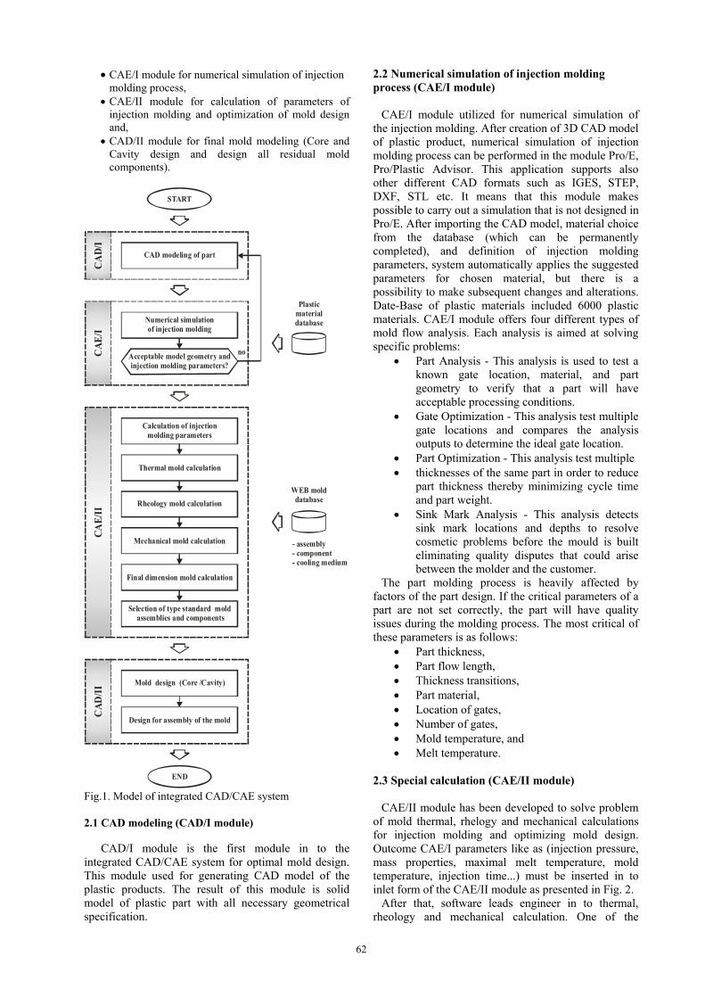
62
CAE/I module for numerical simulation of injection molding process,
CAE/II module for calculation of parameters of injection molding and optimization of mold design and,
CAD/II module for final mold modeling (Core and Cavity design and design all residual mold components).
START
CA
D/I
Plasticmaterial database
CA
E/I
END
Numerical simulation of injection molding
Acceptable model geometry and parameters
?injection molding
CAD modeling of part
Final dimension mold calculation
Selection of type standard mold assemblies and components
Mechanical mold calculation
Rheology mold calculation
Thermal mold calculation
Calculation of parameters
injectionmolding
Design for assembly of the mold
Mold design (Core /Cavity)
CA
E/I
IC
AD
/II
no
WEB mold database
- assembly- component- cooling medium
Fig.1. Model of integrated CAD/CAE system 2.1 CAD modeling (CAD/I module)
CAD/I module is the first module in to the
integrated CAD/CAE system for optimal mold design. This module used for generating CAD model of the plastic products. The result of this module is solid model of plastic part with all necessary geometrical specification.
2.2 Numerical simulation of injection molding process (CAE/I module)
CAE/I module utilized for numerical simulation of the injection molding. After creation of 3D CAD model of plastic product, numerical simulation of injection molding process can be performed in the module Pro/E, Pro/Plastic Advisor. This application supports also other different CAD formats such as IGES, STEP, DXF, STL etc. It means that this module makes possible to carry out a simulation that is not designed in Pro/E. After importing the CAD model, material choice from the database (which can be permanently completed), and definition of injection molding parameters, system automatically applies the suggested parameters for chosen material, but there is a possibility to make subsequent changes and alterations. Date-Base of plastic materials included 6000 plastic materials. CAE/I module offers four different types of mold flow analysis. Each analysis is aimed at solving specific problems:
Part Analysis - This analysis is used to test a known gate location, material, and part geometry to verify that a part will have acceptable processing conditions.
Gate Optimization - This analysis test multiple gate locations and compares the analysis outputs to determine the ideal gate location.
Part Optimization - This analysis test multiple thicknesses of the same part in order to reduce
part thickness thereby minimizing cycle time and part weight.
Sink Mark Analysis - This analysis detects sink mark locations and depths to resolve cosmetic problems before the mould is built eliminating quality disputes that could arise between the molder and the customer.
The part molding process is heavily affected by factors of the part design. If the critical parameters of a part are not set correctly, the part will have quality issues during the molding process. The most critical of these parameters is as follows:
Part thickness, Part flow length, Thickness transitions, Part material, Location of gates, Number of gates, Mold temperature, and Melt temperature.
2.3 Special calculation (CAE/II module)
CAE/II module has been developed to solve problem of mold thermal, rhelogy and mechanical calculations for injection molding and optimizing mold design. Outcome CAE/I parameters like as (injection pressure, mass properties, maximal melt temperature, mold temperature, injection time...) must be inserted in to inlet form of the CAE/II module as presented in Fig. 2.
After that, software leads engineer in to thermal, rheology and mechanical calculation. One of the
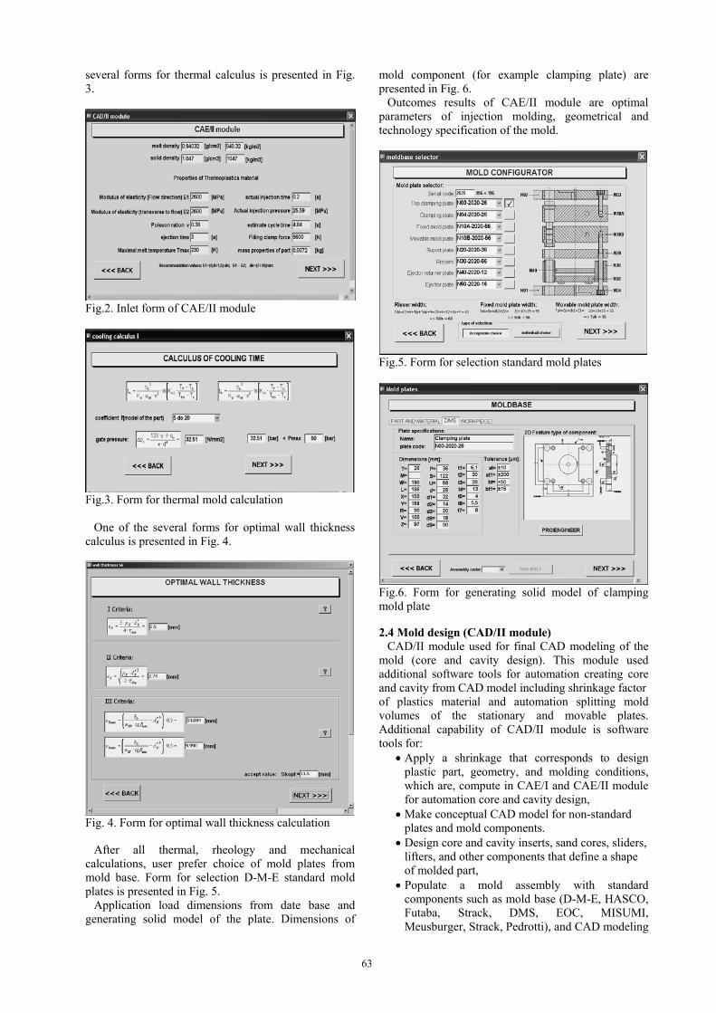
63
several forms for thermal calculus is presented in Fig. 3.
Fig.2. Inlet form of CAE/II module
Fig.3. Form for thermal mold calculation
One of the several forms for optimal wall thickness calculus is presented in Fig. 4.
Fig. 4. Form for optimal wall thickness calculation
After all thermal, rheology and mechanical calculations, user prefer choice of mold plates from mold base. Form for selection D-M-E standard mold plates is presented in Fig. 5.
Application load dimensions from date base and generating solid model of the plate. Dimensions of
mold component (for example clamping plate) are presented in Fig. 6.
Outcomes results of CAE/II module are optimal parameters of injection molding, geometrical and technology specification of the mold.
Fig.5. Form for selection standard mold plates
Fig.6. Form for generating solid model of clamping mold plate 2.4 Mold design (CAD/II module)
CAD/II module used for final CAD modeling of the mold (core and cavity design). This module used additional software tools for automation creating core and cavity from CAD model including shrinkage factor of plastics material and automation splitting mold volumes of the stationary and movable plates. Additional capability of CAD/II module is software tools for:
Apply a shrinkage that corresponds to design plastic part, geometry, and molding conditions, which are, compute in CAE/I and CAE/II module for automation core and cavity design,
Make conceptual CAD model for non-standard plates and mold components.
Design core and cavity inserts, sand cores, sliders, lifters, and other components that define a shape of molded part,
Populate a mold assembly with standard components such as mold base (D-M-E, HASCO, Futaba, Strack, DMS, EOC, MISUMI, Meusburger, Strack, Pedrotti), and CAD modeling
64
ejector pins, screws, and other components creating corresponding clearance holes,
Create runners and waterlines, which dimensions was calculated in CAE/II module,
Check interference of components during mold opening, and check the draft surfaces.
After applied dimensions and selection mold components, CAD/II module generating 3D model of the fixed and movable plate. Geometry mold specifications, which are calculating in CAE/II module, automatically integrated in to CAD/II module, as results CAD/II outcomes are assembly of mold plates. 3. CONCLUSION
In this paper process design of plastic parts production, by means of Pro/E and special application for mold design are presented. As the production, results show the analyses, which have been performed during the process design, prove to be correct, e.g., integrated CAD/CAE system proves to be a confident software tool. All described modules of CAD/CAE system are 3D solid-based, feature oriented, associative and modular. Plastics flow simulation product in CAE/I that allows engineers to determine optimal critical parameters. CAD/II module also enables engineers to capture their own unique design standards and best practices directly within the mold assemblies and components. Module for calculation of mold specification and parameters of injection molding (CAE/II) improves design efficiency, reduce mold design errors, and make need fully information of geometry and technology for complete mold design. Of course, that standard components library (CAD/II) ensures the consistency of mold development and reduces the time and manufacturing cost of standard components. A design decision-making system assists the project leader in making key decisions quickly to guide designers via module.
The future work of this research can focus on two issues. The first one is an intelligent core and mold base with knowledge-based management for automatic parting surface creation, and components assembling through feature-oriented approach and development new high-tech formulas for mold calculation in CAE/II module. 4. REFERENCES [1] Hodolic, J., Matin, I., Stevic, M., Kovačevic, I., Kuric, I.: Mold design and simulation of plastic injection molding process in the CAD/CAE software, 12th International Scientific Conference MECHANICAL ENGINEERING 2008, pp. CDROM, The Faculty of Mechanical Engineering, Bratislava, 13.-14. November 2008. [2] Todic, V., Lukic, D., Stevic, M., Milosevic, M.: Integrated CAPP System for Plastic Injection Molds Manufacturing., Materiale Plastice, Vol. 44, No. 4, pp.381-389, 2008. [3] Godec, D.: Development of systemic theory of mould for injection molding of thermoplastics, Faculty of Mechanical Engineering and Naval Architecture, MSc Thesis, pp. 217, Zagreb, Croatia, 2000.
[4] Kovljenic, B., Ivanovic, R., Puzovic, R., Popovic, M.: The state and perspectives of CAD/CAM/CAE application in plastic products and corresponding tools design, 29th Jupiter Conference, pp. 2.47-2.50., Faculty of Mechanical Engineering, Belgrade, February, 2003. [5] Ren Jong , W., Wu, Ch., Liu, H. H.,. Li, M.Y.: A Collaboration Navigation System for Concurente Mold Design, The International Journal of Advanced Manufacturing Technology, Vol. 40, No. 3-4, pp. 215-225, 2009. [6] Low, M. L. H., Lee, K. S.: Application of standardization for initial design of plasticinjection moulds, International Journal of Production Research, Vol. 41, No. 10, pp. 2301–2324, 2003. [7] Bor-Tsuen Lin, Ming-Ren Chang, Hau-Luen Huang and Chun-Yu Liu.: Computer-aided structural design of drawing dies for stamping processes based on functional features, The International Journal of Advanced Manufacturing Technology, Vol. 42, No. 11-12, pp. 468-479, 2008. [8] Kong, L., Fuh, J. Y. H., Lee, K. S., Liu, X. L., Ling, L. S., Zhang, Y. F., Nee, A. Y. C. A Windows-native 3D plastic injection mold design system, Journal of Materials Processing Technology, Vol. 139, No. 1-3, pp. 81-89, 2003. [9] Matin, I., Hodolic, J., Budak, I.: Injection moulding simulation in the automated product designing systems, International Journal of Simulation Modeling, Vol. 3, No. 2-3, pp 69-79, 2004. [10] Hodolic, J., Matin, I., Vukelic, Dj., Antic, A.: Using compex surfaces for Core and Cavity design of mold, 8th International Scientific Conference - New ways in Manufacturing Technologies, pp. 299-302, Technical University of Košice – Faculty of Manufacturing Technologies with a seat in Prešov, Prešov, 22-23 June, 2006. [11] Lou, Z., Jiang, H., Ruan, X.: Development of Integrated knowlledge-based system for mold-base Design, Journal of Materials Processing Technology, Vol. 150, No. 1-2, pp.194-199, 2004.[12] Lam, Y. C., Britton, G. A., Deng, Y. M.: A computer-aided system for an optimal moulding conditions design using a simulation-based approach, The International Journal of Advanced Manufacturing Technology, Vol. 22, No. 7-8, pp. 574–586, 2003 Authors: MSc. Ivan Matin, Doc. dr. Miodrag Hadzistevic, Prof. dr Janko Hodolic, Mgr. MSc. Djordje Vukelic, University of Novi Sad, Faculty of Technical Sciences, Department for Production Engineering, Trg Dositeja Obradovica 6, 21000 Novi Sad, Serbia, Phone.: ++381 21 485-2350, Fax: ++381 21 454-495. Prof. dr Branko Tadic, University of Kragujevac, Faculty of Mechanical Engineering, Department for Production Engineering, Sestre Janjic 6, 34000 Kragujevac, Serbia, Phone: ++381 34 335 990. E-mail: [email protected] [email protected] [email protected] [email protected] [email protected]
65
Flimel, M.
NEED OF PREDICTIVE ENVIRONMENTAL FRIENDLY SYSTEM OF NOISE PROTECTION
Abstract: This article is about noise protection requirements from industry production in urban environment of the cities. Furthermore it points tools that can be used during proposal phase in order to ensure not only worker, but also inhabitant protection in the surrounding of the industrial facility. As we can see in the article, system approach is very important in this matter. Key words: noise protection, system approach, industry, environment 1. INTRODUCTION Manufacturing is one of the dominant activities and is carried out in interior of building objects and also in exterior within urban build-up area. Manufacturing companies arise by various ways:
as concentrated new buildings (industrial green land)
as new buildings within current build-up area on free parcels
by reconstruction of current non functional manufacturing objects (brown parks)
by reconstruction of various buildings in build-up areas (additional building or superstructure)
Borders of functional urban city zones (living, industrial, transporting, recreational, etc.) are more often loosing and enterprise intentions are in mixed urban city zones. New production brings also negatives in the form of noise and vibrations that have to be solved. Solution is in environmental friendly system of noise protection, which consists of various tools ensuring health, comfort, safety and adequate human’s performance in production process or in surrounding inhabitant’s buildings. The goal of this paper is to point out only on the noise prediction area from the production during the proposal phase. 2. NOISE AND PRODUCTION FLEXIBILITY Many noise sources are influencing human in interior or exterior environment. Every source has different influence on human and therefore noise perception is individual. Sound is acoustic vibration that brings up human perception. Intensity of hearing perception is not linear with intensity of acoustic pressure. Relation between volume and rumble level is dependent on the frequency. Sound (or noise) perception from production itself and noise influence on organism depends on various acoustic and non/acoustic factors like:
noise type produced by sources - the most dangerous is impulse noise, then sustainable
noise, cyclic noise and the less dangerous is interruptible noise,
noise levels - we can divide to relative noise up to 65 dB(A) (influences psychic) and absolute noise over 65 dB(A) which influences vegetative neurons system and hearing organ. Above 120dB(A) causes noise destruction of the hearing organ, pain and impacts central neuros system,
noise frequency – low frequency noise is not dangerous, the higher frequency, the more damage noise can cause,
exposition time of the noise – noise has cumulative character and by rising exposition time also count and seriousness of hearing disorders is increasing,
reference time interval – noise is most unfavorable during night the better it is during evening and day,
individual organism perception, personal disposition of the human – depends on higher neuros activity, genetic factors, age, sex, health state and so on,
from subjective relation to the sound (noise), social and economic factors,
from type of performed activity and surrounding environment
Production activity is the environment of market economy characteristic by frequent changes. Changes are dependent on products demand (volume, type, and speed of production, etc.) which are connected with production devices that are producing noise as side product. Production flexibility is possible not only by assortment change, but also by replacement of production technologies e.g. to less noise one. Flexibility in the time of current global crisis can mean also production depression and by that mean even reduction of environmental noise load. 2. SYSTEM APPROACH IN NOISE PROTECTION Acoustic assessment of protected environment (2 m
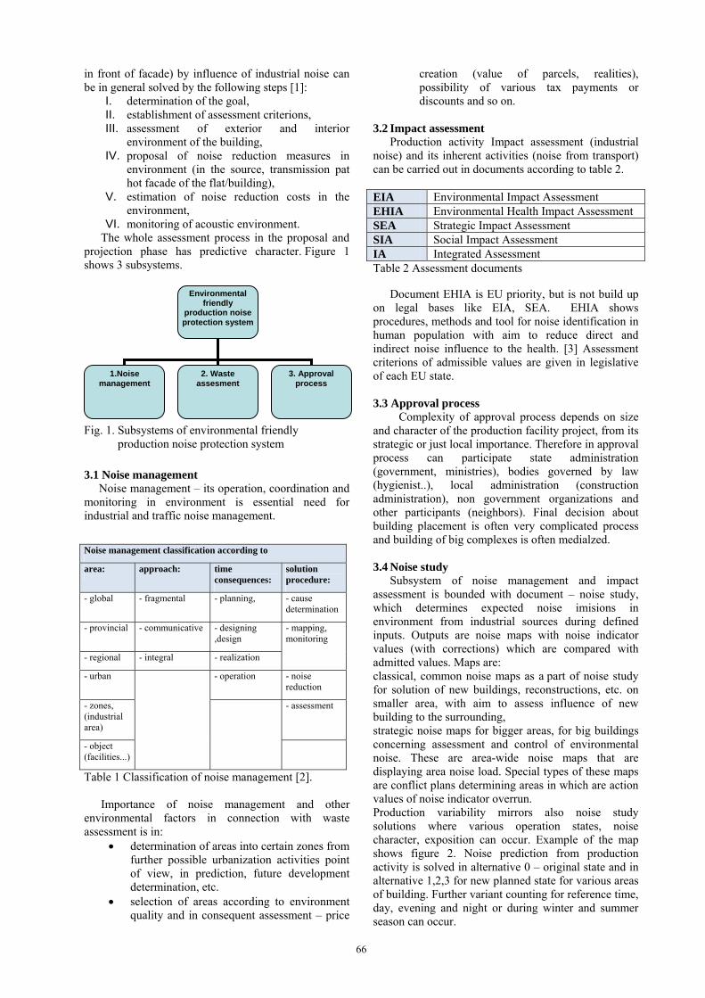
66
in front of facade) by influence of industrial noise can be in general solved by the following steps [1]:
I. determination of the goal, II. establishment of assessment criterions, III. assessment of exterior and interior
environment of the building, IV. proposal of noise reduction measures in
environment (in the source, transmission pat hot facade of the flat/building),
V. estimation of noise reduction costs in the environment,
VI. monitoring of acoustic environment. The whole assessment process in the proposal and projection phase has predictive character. Figure 1 shows 3 subsystems.
Fig. 1. Subsystems of environmental friendly
production noise protection system
3.1 Noise management Noise management – its operation, coordination and monitoring in environment is essential need for industrial and traffic noise management.
Table 1 Classification of noise management [2]. Importance of noise management and other environmental factors in connection with waste assessment is in:
determination of areas into certain zones from further possible urbanization activities point of view, in prediction, future development determination, etc.
selection of areas according to environment quality and in consequent assessment – price
creation (value of parcels, realities), possibility of various tax payments or discounts and so on.
3.2 Impact assessment Production activity Impact assessment (industrial noise) and its inherent activities (noise from transport) can be carried out in documents according to table 2. EIA Environmental Impact Assessment EHIA Environmental Health Impact Assessment SEA Strategic Impact Assessment SIA Social Impact Assessment IA Integrated Assessment Table 2 Assessment documents Document EHIA is EU priority, but is not build up on legal bases like EIA, SEA. EHIA shows procedures, methods and tool for noise identification in human population with aim to reduce direct and indirect noise influence to the health. [3] Assessment criterions of admissible values are given in legislative of each EU state. 3.3 Approval process Complexity of approval process depends on size and character of the production facility project, from its strategic or just local importance. Therefore in approval process can participate state administration (government, ministries), bodies governed by law (hygienist..), local administration (construction administration), non government organizations and other participants (neighbors). Final decision about building placement is often very complicated process and building of big complexes is often medialzed. 3.4 Noise study Subsystem of noise management and impact assessment is bounded with document – noise study, which determines expected noise imisions in environment from industrial sources during defined inputs. Outputs are noise maps with noise indicator values (with corrections) which are compared with admitted values. Maps are: classical, common noise maps as a part of noise study for solution of new buildings, reconstructions, etc. on smaller area, with aim to assess influence of new building to the surrounding, strategic noise maps for bigger areas, for big buildings concerning assessment and control of environmental noise. These are area-wide noise maps that are displaying area noise load. Special types of these maps are conflict plans determining areas in which are action values of noise indicator overrun. Production variability mirrors also noise study solutions where various operation states, noise character, exposition can occur. Example of the map shows figure 2. Noise prediction from production activity is solved in alternative 0 – original state and in alternative 1,2,3 for new planned state for various areas of building. Further variant counting for reference time, day, evening and night or during winter and summer season can occur.
Noise management classification according to
area: approach: time consequences:
solution procedure:
- global - fragmental - planning, - cause determination
- provincial - communicative - designing ,design
- regional - integral - realization
- mapping, monitoring
- urban - operation - noise reduction
- zones, (industrial area)
- assessment
- object (facilities...)
Environmental friendly
production noise protection system
1.Noise management
2. Waste assesment
3. Approval process
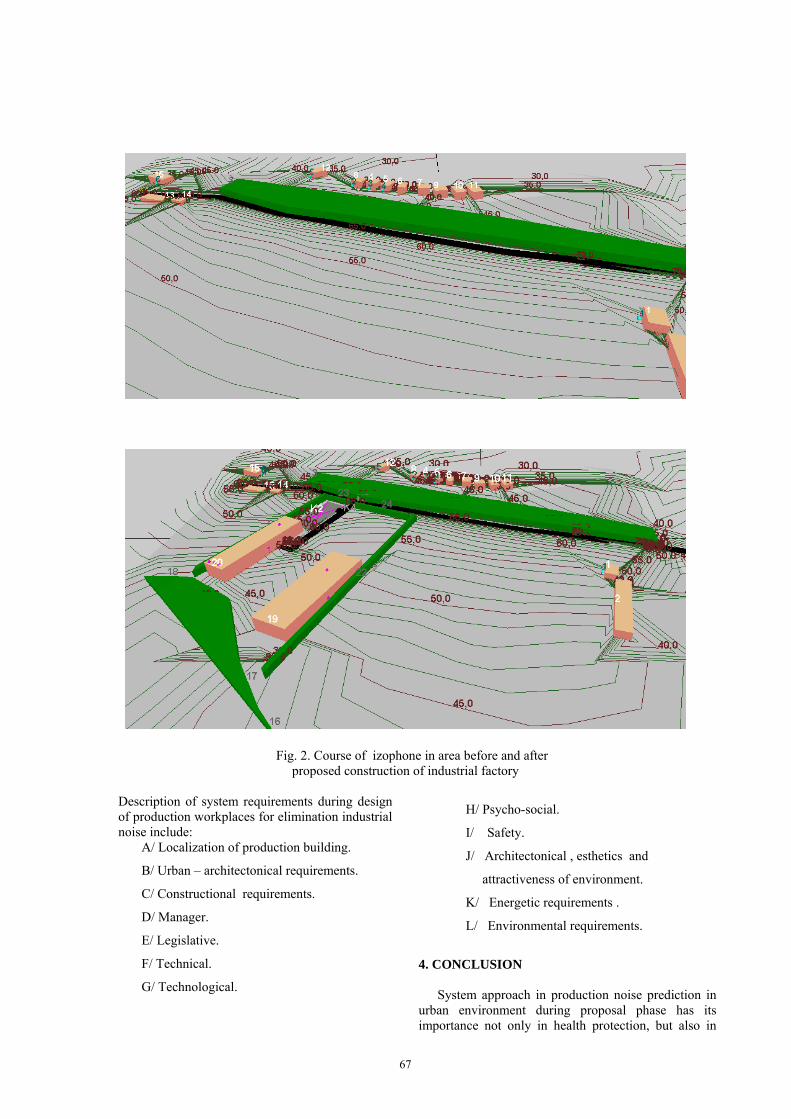
67
Fig. 2. Course of izophone in area before and after proposed construction of industrial factory
Description of system requirements during design of production workplaces for elimination industrial noise include:
A/ Localization of production building.
B/ Urban – architectonical requirements.
C/ Constructional requirements.
D/ Manager.
E/ Legislative.
F/ Technical.
G/ Technological.
H/ Psycho-social.
I/ Safety.
J/ Architectonical , esthetics and
attractiveness of environment.
K/ Energetic requirements .
L/ Environmental requirements.
4. CONCLUSION System approach in production noise prediction in urban environment during proposal phase has its importance not only in health protection, but also in

68
economic area. Costs and measures for noise elimination during proposal phase are lower than additional measures that have to be done during operation of the factory. Environmental friendly system of noise protection applied by manufacturing companies (investors) also rises their image on the market. 5. REFERENCES [1] Žiaran.S..: Akustické hodnotenie chráneného prostredia, In: Zborník z 19.konferencie Vnútorná klíma budov 2008, Tatranská Lesná 2.-3.decembra 2008, s.13-20, ISBN 978-80-89216-26-0 [2] Flimel,M.: Manažerské přístupy k hluku. Moderní řízení, ročník 40, č. 7, 2005, s. 32-33. [3] Koppová.K.: Hodnotenie dopadov na zdravie, Inov.kurz., www.uvzsr.sk Author: doc. Ing. Marián Flimel., CSc., Technical University of Košice, Faculty of Manufacturing Technologies, Bayerova 1, 080 01 Prešov, Slovak Republic Phone.: +421 51 7722-828 E-mail: [email protected]
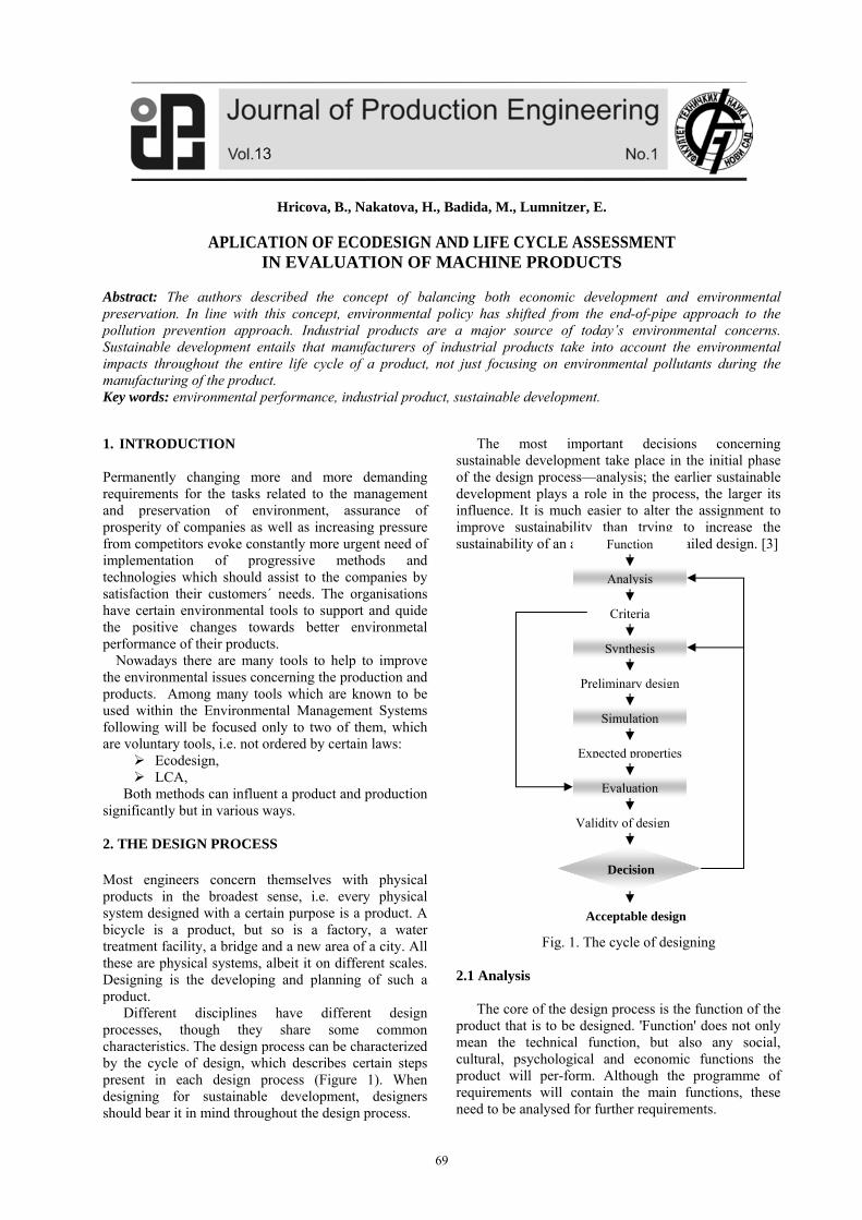
69
Hricova, B., Nakatova, H., Badida, M., Lumnitzer, E.
APLICATION OF ECODESIGN AND LIFE CYCLE ASSESSMENT IN EVALUATION OF MACHINE PRODUCTS
Abstract: The authors described the concept of balancing both economic development and environmental preservation. In line with this concept, environmental policy has shifted from the end-of-pipe approach to the pollution prevention approach. Industrial products are a major source of today’s environmental concerns. Sustainable development entails that manufacturers of industrial products take into account the environmental impacts throughout the entire life cycle of a product, not just focusing on environmental pollutants during the manufacturing of the product. Key words: environmental performance, industrial product, sustainable development. 1. INTRODUCTION
Permanently changing more and more demanding requirements for the tasks related to the management and preservation of environment, assurance of prosperity of companies as well as increasing pressure from competitors evoke constantly more urgent need of implementation of progressive methods and technologies which should assist to the companies by satisfaction their customers´ needs. The organisations have certain environmental tools to support and quide the positive changes towards better environmetal performance of their products.
Nowadays there are many tools to help to improve the environmental issues concerning the production and products. Among many tools which are known to be used within the Environmental Management Systems following will be focused only to two of them, which are voluntary tools, i.e. not ordered by certain laws:
Ecodesign, LCA,
Both methods can influent a product and production significantly but in various ways.
2. THE DESIGN PROCESS Most engineers concern themselves with physical products in the broadest sense, i.e. every physical system designed with a certain purpose is a product. A bicycle is a product, but so is a factory, a water treatment facility, a bridge and a new area of a city. All these are physical systems, albeit it on different scales. Designing is the developing and planning of such a product.
Different disciplines have different design processes, though they share some common characteristics. The design process can be characterized by the cycle of design, which describes certain steps present in each design process (Figure 1). When designing for sustainable development, designers should bear it in mind throughout the design process.
The most important decisions concerning sustainable development take place in the initial phase of the design process—analysis; the earlier sustainable development plays a role in the process, the larger its influence. It is much easier to alter the assignment to improve sustainability than trying to increase the sustainability of an already finished detailed design. [3]
Fig. 1. The cycle of designing
2.1 Analysis
The core of the design process is the function of the product that is to be designed. 'Function' does not only mean the technical function, but also any social, cultural, psychological and economic functions the product will per-form. Although the programme of requirements will contain the main functions, these need to be analysed for further requirements.
Function
Analysis
Criteria
Synthesis
Preliminary design
Simulation
Expected properties
Evaluation
Validity of design
Acceptable design
Decision
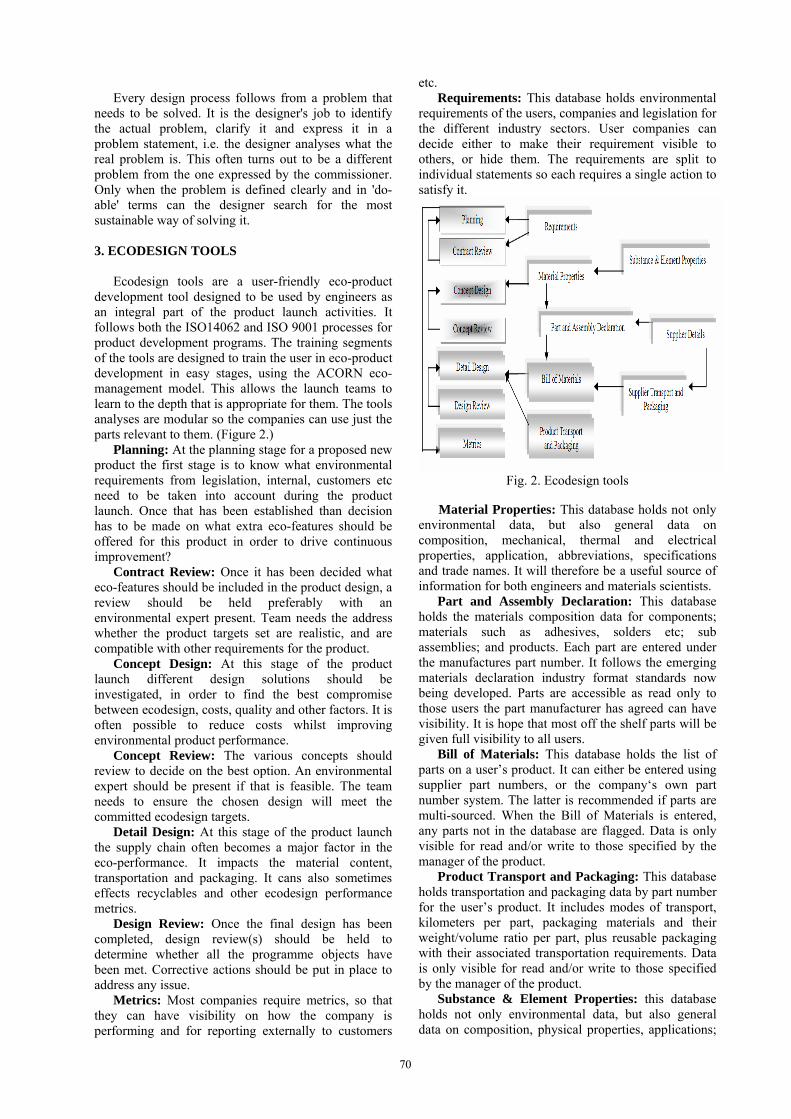
70
Every design process follows from a problem that
needs to be solved. It is the designer's job to identify the actual problem, clarify it and express it in a problem statement, i.e. the designer analyses what the real problem is. This often turns out to be a different problem from the one expressed by the commissioner. Only when the problem is defined clearly and in 'do-able' terms can the designer search for the most sustainable way of solving it.
3. ECODESIGN TOOLS
Ecodesign tools are a user-friendly eco-product
development tool designed to be used by engineers as an integral part of the product launch activities. It follows both the ISO14062 and ISO 9001 processes for product development programs. The training segments of the tools are designed to train the user in eco-product development in easy stages, using the ACORN eco-management model. This allows the launch teams to learn to the depth that is appropriate for them. The tools analyses are modular so the companies can use just the parts relevant to them. (Figure 2.) Planning: At the planning stage for a proposed new product the first stage is to know what environmental requirements from legislation, internal, customers etc need to be taken into account during the product launch. Once that has been established than decision has to be made on what extra eco-features should be offered for this product in order to drive continuous improvement? Contract Review: Once it has been decided what eco-features should be included in the product design, a review should be held preferably with an environmental expert present. Team needs the address whether the product targets set are realistic, and are compatible with other requirements for the product. Concept Design: At this stage of the product launch different design solutions should be investigated, in order to find the best compromise between ecodesign, costs, quality and other factors. It is often possible to reduce costs whilst improving environmental product performance. Concept Review: The various concepts should review to decide on the best option. An environmental expert should be present if that is feasible. The team needs to ensure the chosen design will meet the committed ecodesign targets. Detail Design: At this stage of the product launch the supply chain often becomes a major factor in the eco-performance. It impacts the material content, transportation and packaging. It cans also sometimes effects recyclables and other ecodesign performance metrics. Design Review: Once the final design has been completed, design review(s) should be held to determine whether all the programme objects have been met. Corrective actions should be put in place to address any issue. Metrics: Most companies require metrics, so that they can have visibility on how the company is performing and for reporting externally to customers
etc. Requirements: This database holds environmental
requirements of the users, companies and legislation for the different industry sectors. User companies can decide either to make their requirement visible to others, or hide them. The requirements are split to individual statements so each requires a single action to satisfy it.
Fig. 2. Ecodesign tools
Material Properties: This database holds not only environmental data, but also general data on composition, mechanical, thermal and electrical properties, application, abbreviations, specifications and trade names. It will therefore be a useful source of information for both engineers and materials scientists. Part and Assembly Declaration: This database holds the materials composition data for components; materials such as adhesives, solders etc; sub assemblies; and products. Each part are entered under the manufactures part number. It follows the emerging materials declaration industry format standards now being developed. Parts are accessible as read only to those users the part manufacturer has agreed can have visibility. It is hope that most off the shelf parts will be given full visibility to all users. Bill of Materials: This database holds the list of parts on a user’s product. It can either be entered using supplier part numbers, or the company‘s own part number system. The latter is recommended if parts are multi-sourced. When the Bill of Materials is entered, any parts not in the database are flagged. Data is only visible for read and/or write to those specified by the manager of the product. Product Transport and Packaging: This database holds transportation and packaging data by part number for the user’s product. It includes modes of transport, kilometers per part, packaging materials and their weight/volume ratio per part, plus reusable packaging with their associated transportation requirements. Data is only visible for read and/or write to those specified by the manager of the product. Substance & Element Properties: this database holds not only environmental data, but also general data on composition, physical properties, applications;
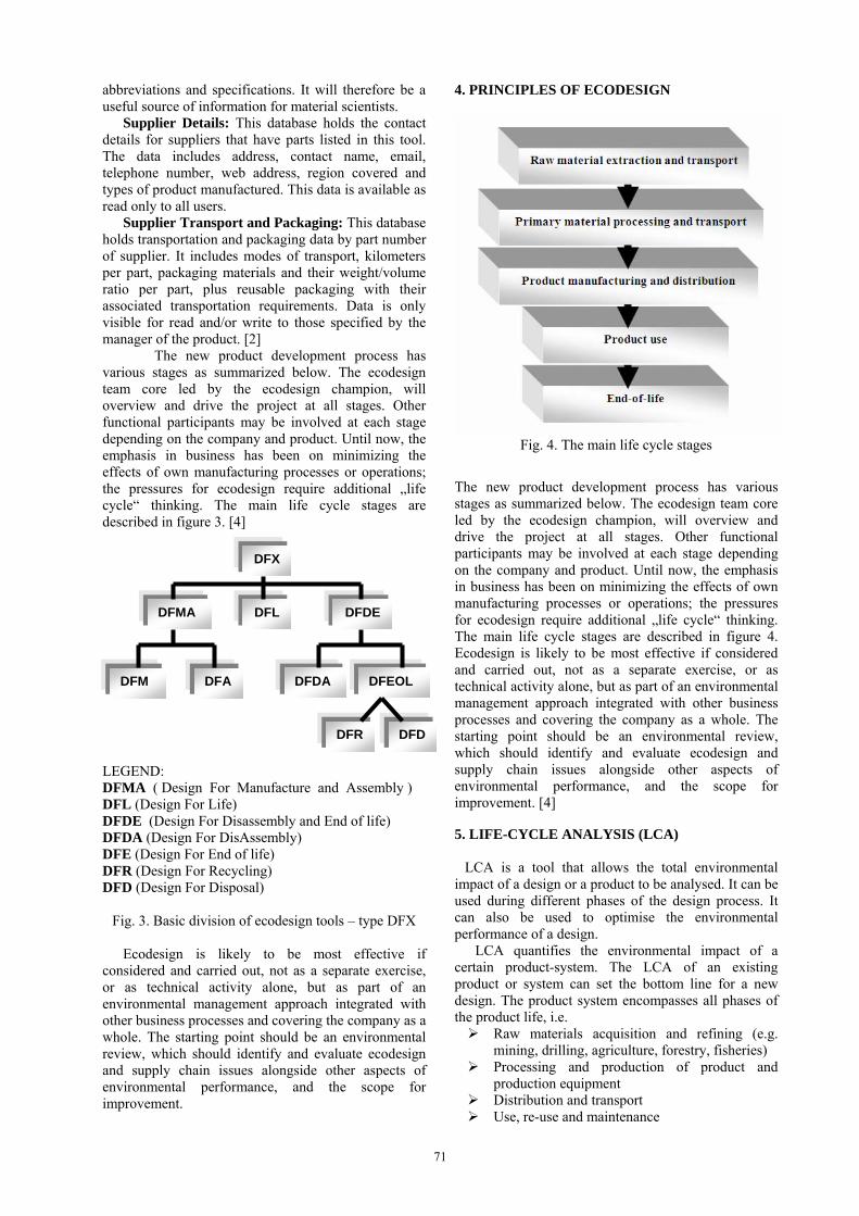
71
abbreviations and specifications. It will therefore be a useful source of information for material scientists. Supplier Details: This database holds the contact details for suppliers that have parts listed in this tool. The data includes address, contact name, email, telephone number, web address, region covered and types of product manufactured. This data is available as read only to all users. Supplier Transport and Packaging: This database holds transportation and packaging data by part number of supplier. It includes modes of transport, kilometers per part, packaging materials and their weight/volume ratio per part, plus reusable packaging with their associated transportation requirements. Data is only visible for read and/or write to those specified by the manager of the product. [2]
The new product development process has various stages as summarized below. The ecodesign team core led by the ecodesign champion, will overview and drive the project at all stages. Other functional participants may be involved at each stage depending on the company and product. Until now, the emphasis in business has been on minimizing the effects of own manufacturing processes or operations; the pressures for ecodesign require additional „life cycle“ thinking. The main life cycle stages are described in figure 3. [4]
LEGEND: DFMA ( Design For Manufacture and Assembly ) DFL (Design For Life) DFDE (Design For Disassembly and End of life) DFDA (Design For DisAssembly) DFE (Design For End of life) DFR (Design For Recycling) DFD (Design For Disposal)
Fig. 3. Basic division of ecodesign tools – type DFX
Ecodesign is likely to be most effective if considered and carried out, not as a separate exercise, or as technical activity alone, but as part of an environmental management approach integrated with other business processes and covering the company as a whole. The starting point should be an environmental review, which should identify and evaluate ecodesign and supply chain issues alongside other aspects of environmental performance, and the scope for improvement.
4. PRINCIPLES OF ECODESIGN
Fig. 4. The main life cycle stages
The new product development process has various stages as summarized below. The ecodesign team core led by the ecodesign champion, will overview and drive the project at all stages. Other functional participants may be involved at each stage depending on the company and product. Until now, the emphasis in business has been on minimizing the effects of own manufacturing processes or operations; the pressures for ecodesign require additional „life cycle“ thinking. The main life cycle stages are described in figure 4. Ecodesign is likely to be most effective if considered and carried out, not as a separate exercise, or as technical activity alone, but as part of an environmental management approach integrated with other business processes and covering the company as a whole. The starting point should be an environmental review, which should identify and evaluate ecodesign and supply chain issues alongside other aspects of environmental performance, and the scope for improvement. [4] 5. LIFE-CYCLE ANALYSIS (LCA)
LCA is a tool that allows the total environmental impact of a design or a product to be analysed. It can be used during different phases of the design process. It can also be used to optimise the environmental performance of a design. LCA quantifies the environmental impact of a certain product-system. The LCA of an existing product or system can set the bottom line for a new design. The product system encompasses all phases of the product life, i.e. Raw materials acquisition and refining (e.g.
mining, drilling, agriculture, forestry, fisheries) Processing and production of product and
production equipment Distribution and transport Use, re-use and maintenance
DFX
DFMA DFL DFDE
DFM DFA DFDA DFEOL
DFR DFD
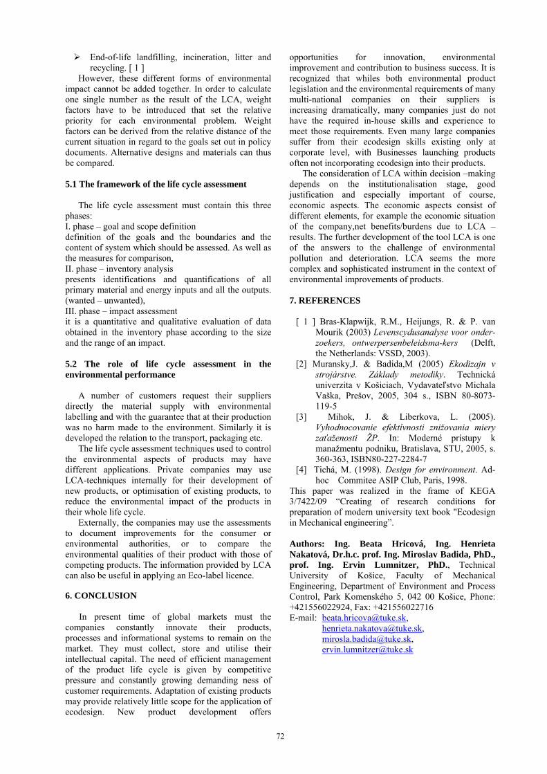
72
End-of-life landfilling, incineration, litter and recycling. [ 1 ]
However, these different forms of environmental impact cannot be added together. In order to calculate one single number as the result of the LCA, weight factors have to be introduced that set the relative priority for each environmental problem. Weight factors can be derived from the relative distance of the current situation in regard to the goals set out in policy documents. Alternative designs and materials can thus be compared. 5.1 The framework of the life cycle assessment The life cycle assessment must contain this three phases: I. phase – goal and scope definition definition of the goals and the boundaries and the content of system which should be assessed. As well as the measures for comparison, II. phase – inventory analysis presents identifications and quantifications of all primary material and energy inputs and all the outputs. (wanted – unwanted), III. phase – impact assessment it is a quantitative and qualitative evaluation of data obtained in the inventory phase according to the size and the range of an impact. 5.2 The role of life cycle assessment in the environmental performance A number of customers request their suppliers directly the material supply with environmental labelling and with the guarantee that at their production was no harm made to the environment. Similarly it is developed the relation to the transport, packaging etc. The life cycle assessment techniques used to control the environmental aspects of products may have different applications. Private companies may use LCA-techniques internally for their development of new products, or optimisation of existing products, to reduce the environmental impact of the products in their whole life cycle. Externally, the companies may use the assessments to document improvements for the consumer or environmental authorities, or to compare the environmental qualities of their product with those of competing products. The information provided by LCA can also be useful in applying an Eco-label licence. 6. CONCLUSION In present time of global markets must the companies constantly innovate their products, processes and informational systems to remain on the market. They must collect, store and utilise their intellectual capital. The need of efficient management of the product life cycle is given by competitive pressure and constantly growing demanding ness of customer requirements. Adaptation of existing products may provide relatively little scope for the application of ecodesign. New product development offers
opportunities for innovation, environmental improvement and contribution to business success. It is recognized that whiles both environmental product legislation and the environmental requirements of many multi-national companies on their suppliers is increasing dramatically, many companies just do not have the required in-house skills and experience to meet those requirements. Even many large companies suffer from their ecodesign skills existing only at corporate level, with Businesses launching products often not incorporating ecodesign into their products. The consideration of LCA within decision –making depends on the institutionalisation stage, good justification and especially important of course, economic aspects. The economic aspects consist of different elements, for example the economic situation of the company,net benefits/burdens due to LCA –results. The further development of the tool LCA is one of the answers to the challenge of environmental pollution and deterioration. LCA seems the more complex and sophisticated instrument in the context of environmental improvements of products. 7. REFERENCES
[ 1 ] Bras-Klapwijk, R.M., Heijungs, R. & P. van Mourik (2003) Levenscydusanalyse voor onder-zoekers, ontwerpersenbeleidsma-kers (Delft, the Netherlands: VSSD, 2003).
[2] Muransky,J. & Badida,M (2005) Ekodizajn v strojárstve. Základy metodiky. Technická univerzita v Košiciach, Vydavateľstvo Michala Vaška, Prešov, 2005, 304 s., ISBN 80-8073-119-5
[3] Mihok, J. & Liberkova, L. (2005). Vyhodnocovanie efektívnosti znižovania miery zaťaženosti ŽP. In: Moderné prístupy k manažmentu podniku, Bratislava, STU, 2005, s. 360-363, ISBN80-227-2284-7
[4] Tichá, M. (1998). Design for environment. Ad-hoc Commitee ASIP Club, Paris, 1998.
This paper was realized in the frame of KEGA 3/7422/09 “Creating of research conditions for preparation of modern university text book "Ecodesign in Mechanical engineering”. Authors: Ing. Beata Hricová, Ing. Henrieta Nakatová, Dr.h.c. prof. Ing. Miroslav Badida, PhD., prof. Ing. Ervin Lumnitzer, PhD., Technical University of Košice, Faculty of Mechanical Engineering, Department of Environment and Process Control, Park Komenského 5, 042 00 Košice, Phone: +421556022924, Fax: +421556022716 E-mail: [email protected],
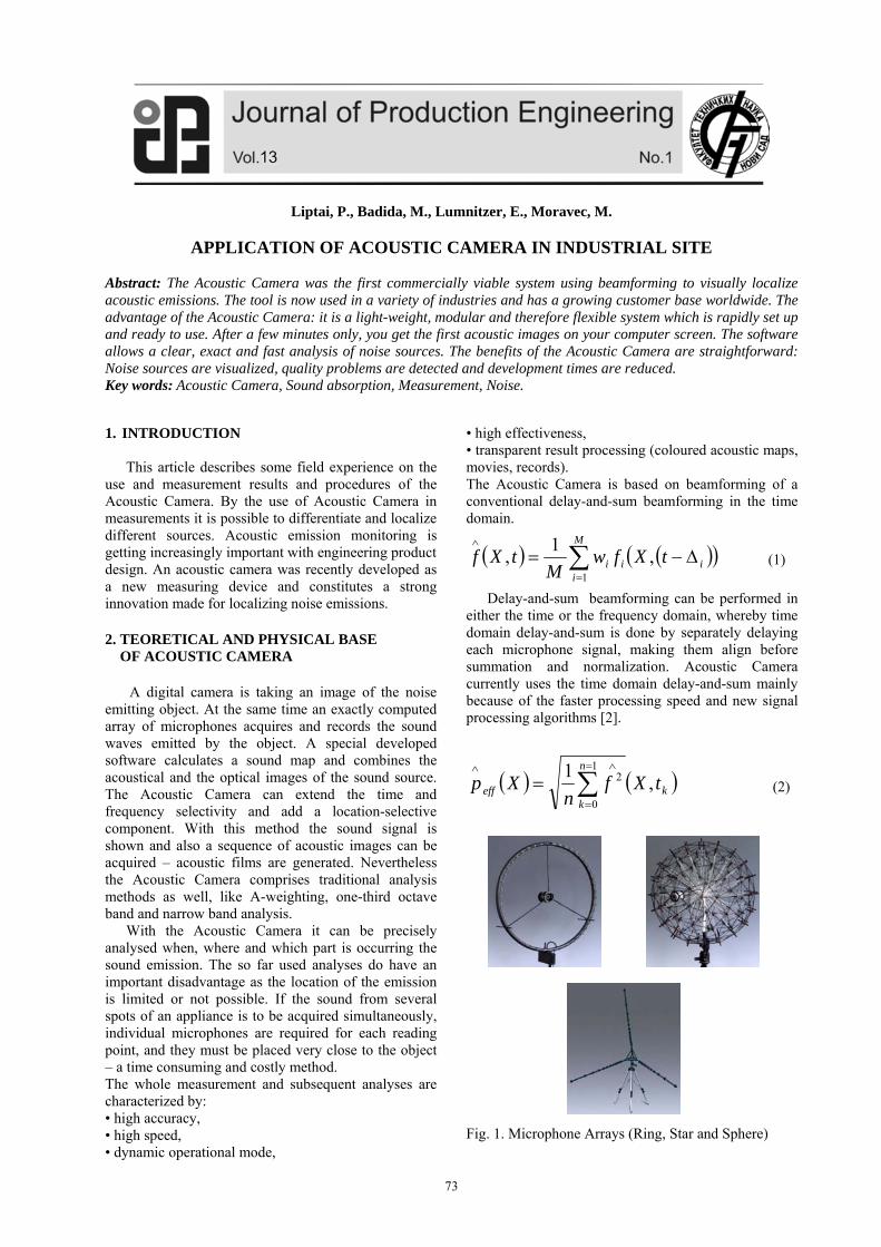
73
Liptai, P., Badida, M., Lumnitzer, E., Moravec, M.
APPLICATION OF ACOUSTIC CAMERA IN INDUSTRIAL SITE Abstract: The Acoustic Camera was the first commercially viable system using beamforming to visually localize acoustic emissions. The tool is now used in a variety of industries and has a growing customer base worldwide. The advantage of the Acoustic Camera: it is a light-weight, modular and therefore flexible system which is rapidly set up and ready to use. After a few minutes only, you get the first acoustic images on your computer screen. The software allows a clear, exact and fast analysis of noise sources. The benefits of the Acoustic Camera are straightforward: Noise sources are visualized, quality problems are detected and development times are reduced. Key words: Acoustic Camera, Sound absorption, Measurement, Noise. 1. INTRODUCTION This article describes some field experience on the use and measurement results and procedures of the Acoustic Camera. By the use of Acoustic Camera in measurements it is possible to differentiate and localize different sources. Acoustic emission monitoring is getting increasingly important with engineering product design. An acoustic camera was recently developed as a new measuring device and constitutes a strong innovation made for localizing noise emissions. 2. TEORETICAL AND PHYSICAL BASE OF ACOUSTIC CAMERA A digital camera is taking an image of the noise emitting object. At the same time an exactly computed array of microphones acquires and records the sound waves emitted by the object. A special developed software calculates a sound map and combines the acoustical and the optical images of the sound source. The Acoustic Camera can extend the time and frequency selectivity and add a location-selective component. With this method the sound signal is shown and also a sequence of acoustic images can be acquired – acoustic films are generated. Nevertheless the Acoustic Camera comprises traditional analysis methods as well, like A-weighting, one-third octave band and narrow band analysis. With the Acoustic Camera it can be precisely analysed when, where and which part is occurring the sound emission. The so far used analyses do have an important disadvantage as the location of the emission is limited or not possible. If the sound from several spots of an appliance is to be acquired simultaneously, individual microphones are required for each reading point, and they must be placed very close to the object – a time consuming and costly method. The whole measurement and subsequent analyses are characterized by: • high accuracy, • high speed, • dynamic operational mode,
• high effectiveness, • transparent result processing (coloured acoustic maps, movies, records). The Acoustic Camera is based on beamforming of a conventional delay-and-sum beamforming in the time domain.
M
iiii tXfw
MtXf
1
,1
, (1)
Delay-and-sum beamforming can be performed in either the time or the frequency domain, whereby time domain delay-and-sum is done by separately delaying each microphone signal, making them align before summation and normalization. Acoustic Camera currently uses the time domain delay-and-sum mainly because of the faster processing speed and new signal processing algorithms [2].
k
n
keff tXf
nXp ,
1 1
0
2
(2)
Fig. 1. Microphone Arrays (Ring, Star and Sphere)
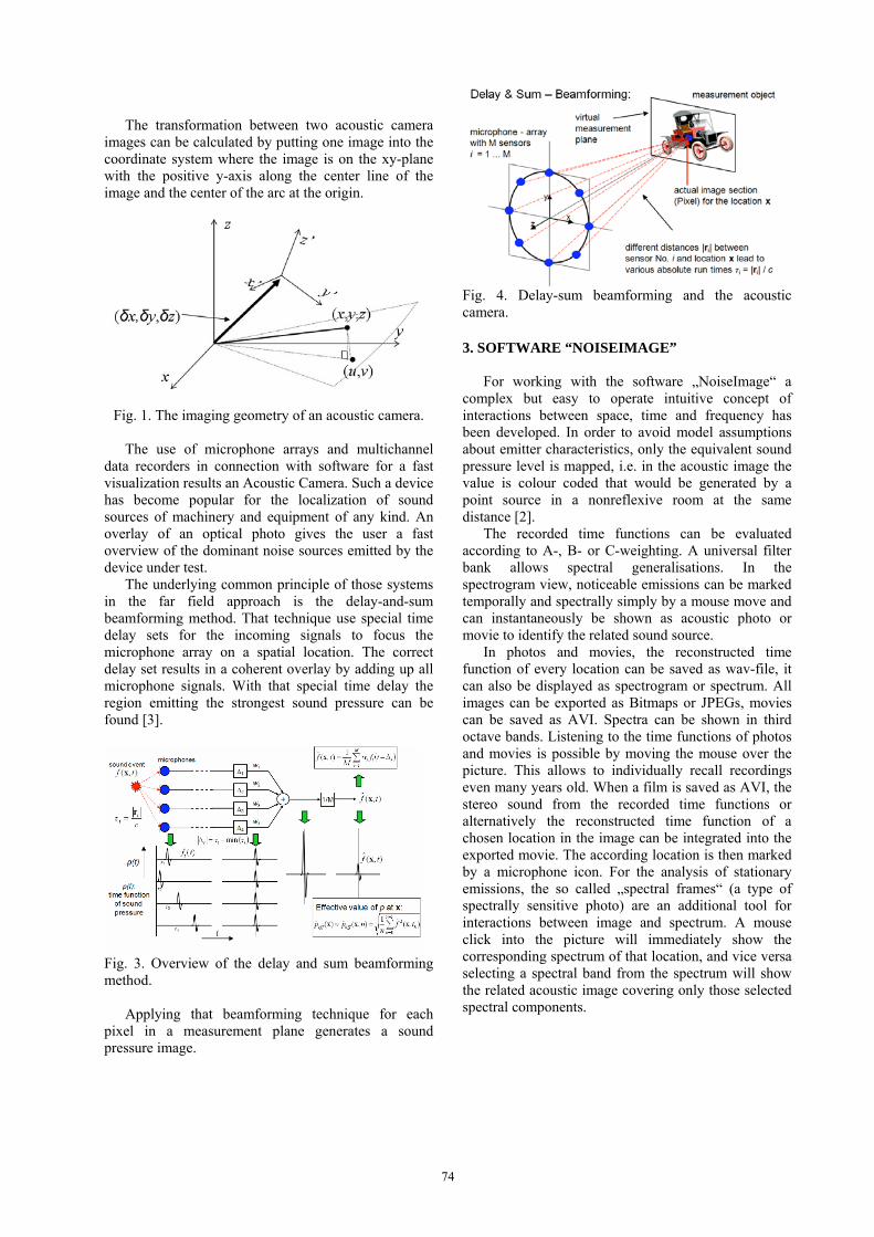
74
The transformation between two acoustic camera images can be calculated by putting one image into the coordinate system where the image is on the xy-plane with the positive y-axis along the center line of the image and the center of the arc at the origin.
Fig. 1. The imaging geometry of an acoustic camera. The use of microphone arrays and multichannel data recorders in connection with software for a fast visualization results an Acoustic Camera. Such a device has become popular for the localization of sound sources of machinery and equipment of any kind. An overlay of an optical photo gives the user a fast overview of the dominant noise sources emitted by the device under test. The underlying common principle of those systems in the far field approach is the delay-and-sum beamforming method. That technique use special time delay sets for the incoming signals to focus the microphone array on a spatial location. The correct delay set results in a coherent overlay by adding up all microphone signals. With that special time delay the region emitting the strongest sound pressure can be found [3].
Fig. 3. Overview of the delay and sum beamforming method. Applying that beamforming technique for each pixel in a measurement plane generates a sound pressure image.
Fig. 4. Delay-sum beamforming and the acoustic camera. 3. SOFTWARE “NOISEIMAGE” For working with the software „NoiseImage“ a complex but easy to operate intuitive concept of interactions between space, time and frequency has been developed. In order to avoid model assumptions about emitter characteristics, only the equivalent sound pressure level is mapped, i.e. in the acoustic image the value is colour coded that would be generated by a point source in a nonreflexive room at the same distance [2]. The recorded time functions can be evaluated according to A-, B- or C-weighting. A universal filter bank allows spectral generalisations. In the spectrogram view, noticeable emissions can be marked temporally and spectrally simply by a mouse move and can instantaneously be shown as acoustic photo or movie to identify the related sound source. In photos and movies, the reconstructed time function of every location can be saved as wav-file, it can also be displayed as spectrogram or spectrum. All images can be exported as Bitmaps or JPEGs, movies can be saved as AVI. Spectra can be shown in third octave bands. Listening to the time functions of photos and movies is possible by moving the mouse over the picture. This allows to individually recall recordings even many years old. When a film is saved as AVI, the stereo sound from the recorded time functions or alternatively the reconstructed time function of a chosen location in the image can be integrated into the exported movie. The according location is then marked by a microphone icon. For the analysis of stationary emissions, the so called „spectral frames“ (a type of spectrally sensitive photo) are an additional tool for interactions between image and spectrum. A mouse click into the picture will immediately show the corresponding spectrum of that location, and vice versa selecting a spectral band from the spectrum will show the related acoustic image covering only those selected spectral components.

75
Fig. 5. Spektrum of measuring data.
Fig. 6. Spektrogram of measuring data. The spectrogram is used to generate acoustic photos by studying tonal components and to easily do filtering including playback of selected area, so that the display/generation of the acoustic photo is optimized.
Fig. 7. Spektrogram of measuring data with shining critical frequency.
4. EXPERIMENTAL MEASUREMENTS IN WORK EXPERIENCE
Fig. 8. Installed Acoustic Camera by exhaust plant.
Fig. 9. Acoustic photo of exhaust plant. In the Acoustic Photo each of the pixels have a corresponding spectra, it is therefore possible to display the spectra for every pixel in the photo. Vice versa another useful post-processing algorithm is the “Spectral Frames”, where it is possible to do the opposite. For every part in the frequency spectra it is possible to mark an area and then to display the corresponding location for this part.
Fig. 10. Installed Acoustic Camera by crushing plant.
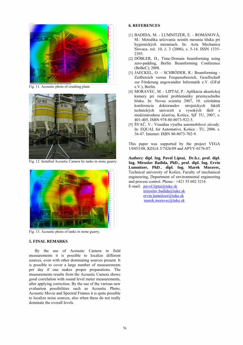
76
Fig. 11. Acoustic photo of crushing plant.
Fig. 12. Installed Acoustic Camera by tanks in stone guarry.
Fig. 13. Acoustic photo of tanks in stone guarry. 5. FINAL REMARKS By the use of Acoustic Camera in field measurements it is possible to localize different sources, even with other dominating sources present. It is possible to cover a large number of measurements per day if one makes proper preparations. The measurements results from the Acoustic Camera shows good correlation with sound level meter measurements, after applying correction. By the use of the various new evaluation possibilities such as Acoustic Photo, Acoustic Movie and Spectral Frames it is quite possible to localize noise sources, also when these do not really dominate the overall levels.
6. REFERENCES [1] BADIDA, M. - LUMNITZER, E. - ROMÁNOVÁ,
M.: Metodika určovania neistôt merania hluku pri hygienických meraniach. In: Acta Mechanica Slovaca. roč. 10, č. 3 (2006), s. 5-14. ISSN 1335-2393.
[2] DÖBLER, D., Time-Domain beamforming using zero-padding, Berlin Beamforming Conference (BeBeC), 2008.
[3] JAECKEL, O. – SCHRÖDER, R.: Beamforming - Zeitbereich versus Frequenzbereich, Gesellschaft zur Förderung angewandter Informatik e.V. (GFaI e.V.), Berlin.
[4] MORAVEC, M. - LIPTAI, P.: Aplikácia akustickej kamery pri riešení problematiky priemyselného hluku. In: Novus scientia 2007, 10. celoštátna konferencia doktorandov strojníckych fakúlt technických univerzít a vysokých škôl s medzinárodnou účasťou, Košice, SjF TU, 2007, s. 401-405, ISBN 978-80-8073-922-5.
[5] ŠVAČ, V.: Vizuálna výučba automobilové závody. In: EQUAL for Automative. Košice : TU, 2006. s. 36-47. Internet: ISBN 80-8073-702-9.
This paper was supported by the project VEGA 1/0453/08, KEGA 3/7426/09 and APVV-0176-07. Authors: dipl. Ing. Pavol Liptai, Dr.h.c. prof. dipl. Ing. Miroslav Badida, PhD., prof. dipl. Ing. Ervin Lumnitzer, PhD., dipl. Ing. Marek Moravec, Technical university of Košice, Faculty of mechanical engineering, Department of environmental engineering and process control. Phone.: +421 55 602 3216 E-mail: [email protected] [email protected] [email protected] [email protected]
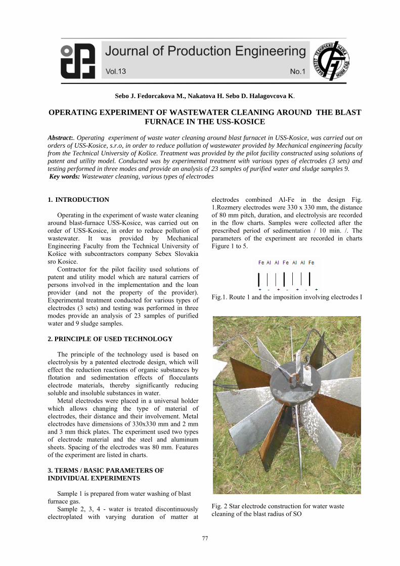
77
Sebo J. Fedorcakova M., Nakatova H. Sebo D. Halagovcova K. OPERATING EXPERIMENT OF WASTEWATER CLEANING AROUND THE BLAST
FURNACE IN THE USS-KOSICE Abstract:. Operating experiment of waste water cleaning around blast furnacet in USS-Kosice, was carried out on orders of USS-Kosice, s.r.o, in order to reduce pollution of wastewater provided by Mechanical engineering faculty from the Technical University of Košice. Treatment was provided by the pilot facility constructed using solutions of patent and utility model. Conducted was by experimental treatment with various types of electrodes (3 sets) and testing performed in three modes and provide an analysis of 23 samples of purified water and sludge samples 9. Key words: Wastewater cleaning, various types of electrodes 1. INTRODUCTION Operating in the experiment of waste water cleaning around blast-furnace USS-Kosice, was carried out on order of USS-Kosice, in order to reduce pollution of wastewater. It was provided by Mechanical Engineering Faculty from the Technical University of Košice with subcontractors company Sebex Slovakia sro Kosice. Contractor for the pilot facility used solutions of patent and utility model which are natural carriers of persons involved in the implementation and the loan provider (and not the property of the provider). Experimental treatment conducted for various types of electrodes (3 sets) and testing was performed in three modes provide an analysis of 23 samples of purified water and 9 sludge samples. 2. PRINCIPLE OF USED TECHNOLOGY The principle of the technology used is based on electrolysis by a patented electrode design, which will effect the reduction reactions of organic substances by flotation and sedimentation effects of flocculants electrode materials, thereby significantly reducing soluble and insoluble substances in water. Metal electrodes were placed in a universal holder which allows changing the type of material of electrodes, their distance and their involvement. Metal electrodes have dimensions of 330x330 mm and 2 mm and 3 mm thick plates. The experiment used two types of electrode material and the steel and aluminum sheets. Spacing of the electrodes was 80 mm. Features of the experiment are listed in charts. 3. TERMS / BASIC PARAMETERS OF INDIVIDUAL EXPERIMENTS Sample 1 is prepared from water washing of blast furnace gas. Sample 2, 3, 4 - water is treated discontinuously electroplated with varying duration of matter at
electrodes combined Al-Fe in the design Fig. 1.Rozmery electrodes were 330 x 330 mm, the distance of 80 mm pitch, duration, and electrolysis are recorded in the flow charts. Samples were collected after the prescribed period of sedimentation / 10 min. /. The parameters of the experiment are recorded in charts Figure 1 to 5.
Fig.1. Route 1 and the imposition involving electrodes I
Fig. 2 Star electrode construction for water waste cleaning of the blast radius of SO
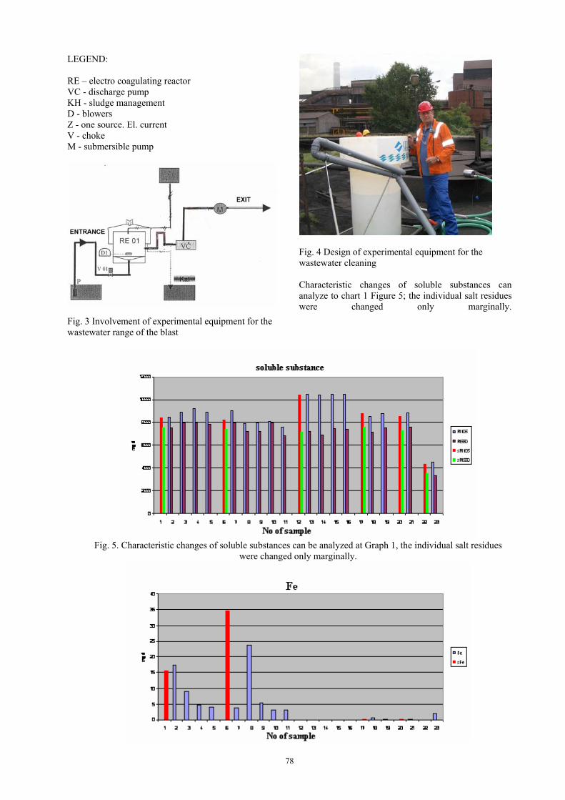
78
LEGEND: RE – electro coagulating reactor VC - discharge pump KH - sludge management D - blowers Z - one source. El. current V - choke M - submersible pump
Fig. 3 Involvement of experimental equipment for the wastewater range of the blast
Fig. 4 Design of experimental equipment for the wastewater cleaning Characteristic changes of soluble substances can analyze to chart 1 Figure 5; the individual salt residues were changed only marginally.
Fig. 5. Characteristic changes of soluble substances can be analyzed at Graph 1, the individual salt residues
were changed only marginally.
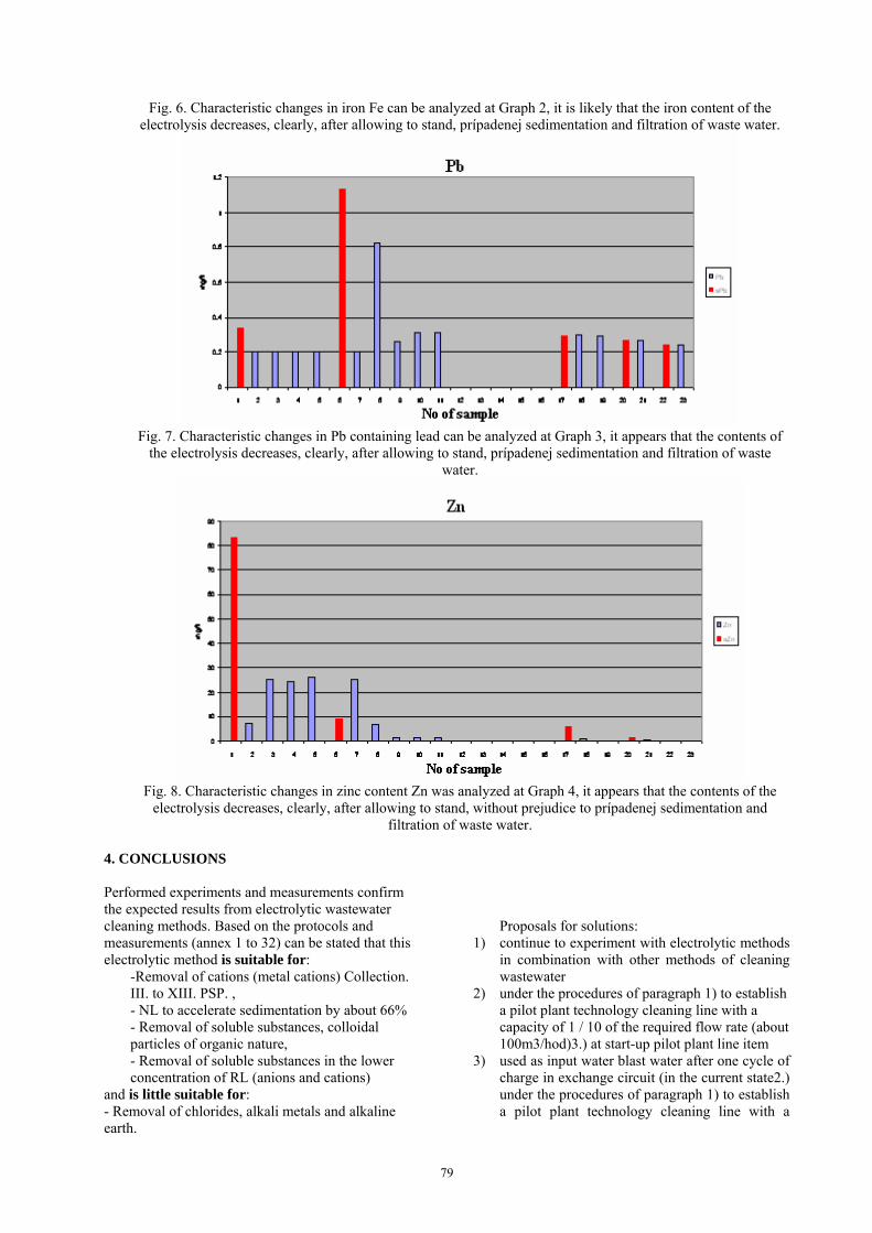
79
Fig. 6. Characteristic changes in iron Fe can be analyzed at Graph 2, it is likely that the iron content of the
electrolysis decreases, clearly, after allowing to stand, prípadenej sedimentation and filtration of waste water.
Fig. 7. Characteristic changes in Pb containing lead can be analyzed at Graph 3, it appears that the contents of
the electrolysis decreases, clearly, after allowing to stand, prípadenej sedimentation and filtration of waste water.
Fig. 8. Characteristic changes in zinc content Zn was analyzed at Graph 4, it appears that the contents of the
electrolysis decreases, clearly, after allowing to stand, without prejudice to prípadenej sedimentation and filtration of waste water.
4. CONCLUSIONS Performed experiments and measurements confirm the expected results from electrolytic wastewater cleaning methods. Based on the protocols and measurements (annex 1 to 32) can be stated that this electrolytic method is suitable for:
-Removal of cations (metal cations) Collection. III. to XIII. PSP. , - NL to accelerate sedimentation by about 66% - Removal of soluble substances, colloidal particles of organic nature, - Removal of soluble substances in the lower concentration of RL (anions and cations)
and is little suitable for: - Removal of chlorides, alkali metals and alkaline earth.
Proposals for solutions:
1) continue to experiment with electrolytic methods in combination with other methods of cleaning wastewater
2) under the procedures of paragraph 1) to establish a pilot plant technology cleaning line with a capacity of 1 / 10 of the required flow rate (about 100m3/hod)3.) at start-up pilot plant line item
3) used as input water blast water after one cycle of charge in exchange circuit (in the current state2.) under the procedures of paragraph 1) to establish a pilot plant technology cleaning line with a

80
capacity of 1 / 10 of the required flow rate (about 100m3/hod)
4) at start-up pilot plant line item 2) used as input water blast water after one cycle of charge in exchange circuit (in the current state
5. LITERATURA [1] BADIDA, M., MAJERNÍK, M., ŠEBO, D.
HODOLIČ J.: Strojárska výroba a životné prostredie, Vienala, ISBN 80-7099-695-1, Košice, 2001,
[2] ŠEBO, D., HRÁDOCKÝ, L., KRÁLIKOVÁ, R.: Nekonvenčný spôsob čistenia odpadových vôd v tepelnej energetike. AtaP JOURNAL, Banská Bystrica, 1998, č. 8.
[3] BADIDA, M., ŠEBO, D. MAJERNÍK, M., MOLNÁR, P.: Multifunkčné elektrokoagulačné čistenie odpadových vôd v priemysle, Strojárstvo, ISNN 1335 2938, č. 2/1999,
[4] MAJERNÍK, M., ŠEBO, D., MOLNÁR, P.: Účinnosť elektrokoagulačného čistenia odpadových vôd v celulózovo-papiernickom priemysle. Strojárstvo, ISNN 1335 2938, č. 4/2000,
[5] ŠEBO, D., PAULÍKOVÁ A.: Likvidácia a úprava technických a technologických kvapalín. . Strojárstvo, ISNN 1335 2938, č. 11/2003,
Authors: Šebo J. PhD., Fedorcakova M. Henrieta Nakatová, Dr.h.c. prof. Ing. Sebo D., Halagovcova K., Technical University of Košice, Faculty of Mechanical Engineering, Department of Environment and Process Control, Park Komenského 5, 042 00 Košice, Phone: +421556022924, Fax: +421556022716
E-mail: [email protected]

107
Prof. Pavel Kovač, PhD, MEng. Borislav Savković, MSc. Assistant
FACULTY OF TECHNICAL SCIENCES Department for Production Engineering Trg Dositeja Obradovica 6
21000 Novi Sad Serbia
Tel.: (+381 21) 485 23 24; 485 23 20 ; 450 366; Fax: (+381 21) 454 495 E-mail: [email protected] http://www.ftn.uns.ac.rs/mma2009
No. of pages: 4 DIN A4 pages Margins: left: 2,5 cm right: 2 cm top: 2 cm bottom: 2 cm Font: Times New Roman Title: Bold 12, capitals Abstract: Italic 10 Headings: Bold 10, capitals Subheadings: Bold 10, small letters Text: Regular 10 Columns: Equal column width with 0,7 cm spacing Spacing: Single line spacing Formulae: Centered and numerated from 1 in ascending order.
Equations must be typed in Equation Editor, with following settings: Style>Math – Times New Roman Size>Full 12pt, Subscript/Superscript 7pt, Symbol 18 pt
Figures: High quality, numerated from 1 in ascending order (e.g.: Fig.1, Fig. 2 etc.); Figures and tables can spread over both two columns, please avoid photographs and colour prints
Tables: Numerated from 1 in ascending order (e.g..: Tab. 1, Tab. 2, etc.)
References: Numerated from [1] in ascending order; cited papers should be marked by the number from the reference list (e.g. [1], [2, 3] ...)
Submission: Papers prepared in MS Word format should be e-mailed to: [email protected], [email protected], [email protected]
Notice: Papers are to be printed in Journal of Production Engineering Sample paper with detailed instructions can be found at: www.ftn.uns.ac.rs/mma2009
INSTRUCTIONS FOR CONTRIBUTORS
FOR MORE INFORMATION, PLEASE CONTACT:


Novi Sad, 2010
9 7 7 1 8 2 1 4 9 3 0 0 5
ISSN 1821-4932
Volume 13 No.1
UNIVERSITY OF NOVI SADFaculty of Technical Sciences
Department of Production EngineeringNOVI SAD, SERBIA
UDK 621 ISSN 1821-4932
J O U R N A L O F
PRODUCTION ENGINEERING
JO
UR
NA
L O
F P
RO
DU
CT
IO
N E
NG
IN
EE
RIN
G, V
ol.13, N
o.1, 2010
JO
UR
NA
L O
F P
RO
DU
CT
IO
N E
NG
IN
EE
RIN
G, V
ol.13, N
o.1, 2010