~OIJ)S’1’IHN IU1’ Al.. - ]

Sate.llit c Radar lnt Crfcronmt ry for Monitoring lcc-shc.c.t Motion:

Application to an Antarctic ICC Stream

Richarcl M, Goldstein, 1 lermann lhgelhardt, Barclay Kamb

and Richard M. 1 ~rolicbl

Abstract

As a new means of monitoring the flow velocities and grounding-line positions of ice

streams, which are indicators of response of the Antarctic and Greenland ice sheets to climatic

change or internal instability, the method of satellite radar interfcrometry (SRI) is here proposed

and app]iccl to the Rutford Ice Stream, Antarctica. ‘J’hc method uses phase comparison of the

radar signal obtained for a pair of SAR images taken a few clays apart to plot an interferogram

which directly displays relative ground motions that have occurred in the time interval between

images. “1’he cletcction limit is about 1.5 mm for vertical motions and about 4 mm for horizontal

motions in the radar beam direction. in the Rutford Ice Stream, SRI velocities agree fairly well

wiih earlier ground-truth data over a longitudinal inlerval of 29 km; the comparison suggests a

secular clccrcase in velocity of about 2% from 1978-80 to 1992. Ungrounded ice is revealed by

large ( -2 m) vertical motions due to tidal uplift, and the grounding line can be mapped at a

rcsolut ion of ca. 0,5 km from the S1{1 interfcrogram. ‘J’he mapped configuration implies

grounding line retreat of 1 to several km since 1980.

11< Go]dstcin, Jet Propulsion 1.aboratory, California lnslitutc of Technology, l’asadcna, CA91 109; 11, Engclhardt and 11. Kan~b, Division of Geological and l’lanctary Sciences, Californialnstitutc of ‘J’echno]ogy, l}asadcna, CA 91 12.S; R. l~rolich, British Antarctic Survey, Cambridge,lJK C113 01;1’.

&) IJK1’I~IN 1;’1’ AI/. -2

]nt reduction

‘J’hc continuing current at[cnticm to the possible response of the polar ice sheets 10 global

climatic change ancl/or internal instability ics (], 2,.?) cn@asi7Jcs the need for ccmt inuccl and if

possible improved ice-sheet monitoring capabilities that can detect significant changes if and as

they develop. Satellite monitoring of ice volume by precision altimetry of the ice-sheet surface

is a promising technique that has just begun to yield results (4). Also needed is monitoring of

ice flow velocities and the position of ice grounding lines, which relate closely to the possibility

of icc-sheet disintegration: a marine-based ice sheet, like the West Antarctic ice sheet, whose

base in its central part lies well below sca level, is subject to a type of instability in which

grounding-line retreat leads to rapid outflow and icc-sheet collapse (5). For monitoring flow,

the usefulness of satellite optical imaging has rcccntly been showJ~ by Bindschadlcr ancl Scambos

(2). We here present a new satellite radar tcchni(Juc for determining ice flow velocity and also

grounding line position, ancl wc show its application to a large, rapidly flowing Antarctic ice

stream.

“J’hc Antarctic ice streams (6) arc fast-moving currents 30-80 km wide, and up to 500 km

king, within the generally slow-moving icc sheet. Thcy reach flow speeds of -800 m a- ],

which arc -100 times faster than the adjacent ice sheet (2,6). Because of the large ice flux that

they carry, the ice streams make the major contribution ( - 90%) to outflow from the icc sheet;

if they were to speed up and/or widen sufficicntl y, they COUIC1 bcccmc the immediate cause of

ice- sheet collapse (5’, 7). Monitoring the extent and motions of the ice streams is therefore of

much importance in assessing ice sheet behavior. It can also contribute to the cmgoing search

for the physical mechanism of ice stream motion (6,6’), on the basis of which attempts to predict

ice stream behavior arc being maclc (5’).

GOl .IX’I’IHN IL-l’ Al,. - q

The possibility of icc-stmm monitoring by the new technique is illustrated with the

Rutford Ice Stream, which is onc of the main outlets of the West Antarc[ic ice sheet, draining

a large area around the 1 lllsworlh Mountains and emptying into the head of the Rome Ice Shelf

(9), IIccausc some ground and satellite data arc already available for it (9,10,11,12), the

Rutford ICC Stream is an advantageous target for applying the new monitoring technique.

Salcllitc Radar lntdcromdry (SRI)

Satellite-bomc imaging synthetic-aperture radar (SAR), such as that current] y provided

by satellite 111{ S- 1 of the liuropcan Space Agency, presents the opportunity for measuring surface

displacement fields interferometricall y by making use of the coherence of the radar beam in the

following way (13). If two radar observations of the same scene are made from locations

sufficiently close together, interference bctwccn the two resulting SAR images can bc obtained

by comparing the phase of the synthesized signals making up the two images. As originally

calculated from

images”) by the

the radar return these images, called “single-look complex images” (“S1 .C

lh]ropcan Space Agency, contain both anlJ~litu(lc anti phase information. 1 lcrc

wc call thcm complex images. 1 n such an image the amplitude and phase at each pixel are given

in the form of a comp]ex number, from which the phase shifl from image ] to image 2 at each

pixc] can bc cxtractcd. “1’hc result is displayed in an “intcrfcrogram” of the image pair (l;ig. 1),

which is an arcal plot of tbc phase shift,

throughout the image.

At any point in the intcrfcrogram

spectrally color coclcd, as a function of position

the phase shifl is a measure of the line-of-sight

component of displaccnwnt of the corresponding ground surface point in relation to the

spacecraf[ from the time of onc image to the other. 1 lalf a wavelength of displacement (2,8 cnl

~iol JEH’10N IH’ Al.. -4

in the example here) produces a phase shifl of 360°. The actual zero of the phase shift is

arbitrary, hcncc only displacements of one point relative to another in the field of view arc

determined. If in traversing Ihc fringe pat[em in 1 ~ig. 1 wc pass from purple through blue and

yellow to red and then to purple, we have passed through a change in phase shift by 360°

direct ion that corresponds to the scatlcrin~ points having moved 2.8 cm relative] y closer

spacecraft from the time of the first image to the scconcl,

in the

to the

SRI’s resolution of displacements depends on the magnitude of the phase noise, which

in IJig, 1 can bc evaluated in areas of broad, widely spacccl fringes, where the r.m. s. scatter in

phase shif

1.3 mm.

is found to bc 17°. 3’his corresponds to a line-of-sight clisplaccmcnt resolution of

]n comparison, the pixel size, which is what limits the resolution in non-

intcrfcrometric imaging mcthocls for measuring ground displaccmnt (2,14), is ca. 65 m,

III order to obtain an SRI interfcrogram like liig. 1 it is ncccssary to bring the two

complex images into sufficiently good pixel-to-pixel registry by shifting one imag,c. relative to

the other! This is done by means of a correlation algorithm (15). Once the registry position is

established, a step of data averaging and condensation is introduced (16). Before calculating the

intcrfcrogram a correction ~~1 – ~)z is made to the phase shift at each pixel to remove a phase shift

that arises not from ground motion but because the spacecraft was not at exactly the same

position when the radar data for the two complex images were obtained. The geometry is shown

in l;ig. 2. The phase shif[

spacecraft positions 1 and 2

is

c#~l -~~1 (in radians) between scattered waves returning to the two

from a given far-dis[an( scattering point at an angle O to the vcr[ical

\,.

.

(bl .I)STliIN 1;1’ Al.. -5

~,p - @l= !: (V COSO - 1) sinO) (1)

where V and 11 are the vertical and horizontal components of spacecraf[ position 2 relative to

position 1 as dcfinccl in l~ig. 2, (17). ‘J’hc radar wavelength is A (=-5.656 cm in the case of I Jig.

1). The inclination angle 0 runs from 19.9° to 26.6° in going from bot[om to top in l~ig. 1.

in principle, phase ciifferenccs of the same type will arise from variations in elevation of

the ground surface in the imaged area, but wc can show that they are ncg]igible for

intcrferograms of low-relief terrain (such as icc shccls and icc streams) obtained with a small

scparat ion between spacecraft positions 1 ancl 2 (small l] and 10. 1 ‘ig. 3 shows the geometry.

Thc change in phase shift A(d~2 – 4)1) for waves scattcrcd frol~~, saY, a nlountain toP at elcvatiol~

z, in relation to ~}2 –~~1 for scattering from the datum level z =-0 at the same map-position, is

obtainab]c from cqn. (1) by allowing O to change by the amount AO =- (z/p) sinO, where p is the

slant range as shown in l~ig. 3; AU can bc treated as infinitesimal, because, for the ccmclitions

of 1 ;ig. 1, z< 100 m while p G 850 km (18). Wc calculate from eqn. (1) a chanp,c in phase shifl

of g ().50 for an c]cvatio]~ z < I ()() m. This amounts to a change of less than 0,2% of Onc fringe,

much smaller than the

Application of S1<1 to

range of observed phase shifts (- 100 fringes) in liig. 1.

the Rut ford lcc Stream

1 ‘ig. 4 is a ncar]y conventional

the 35-knl-wide Rutford ICC Stream

approximately up, the a~,inmth of the

SAR image (19), 100 km by 49 km, showing a par[ of

ccntcrcd at lat. 78043’S, long. 83 °0’W. North is

radar line of sight (botlom to top in the figure) being

350.8°. in 1 jig. 4 the ice s[rcam extends from top to lower right (rouphly north to south)

through the central part of the image, and the bright bands to the left and right arc its marginal

(iOIJ)S”I’li[N IY1’ Al. -6

shear mnes, whm radar reflections from numerous ice-air interfaces in these crevassed zones

givcabright radar return. Asit~lilar higl]radar reflectivity fro~]lc]cvassed] ]lalgillalsl lcar?o~]cs

is observed for ice streams of the Siplc Coast region (20). At the lower left in Irig. 4, the

Minnesota Glacier enters the ice stream from the west, and at the upper left the irregular bright

area west of the ice stream is the lilowcrs IIills, on the cast sick of the IHlsworth Mountains.

‘J’ypical “flow bancls” -- highly elongate surface ridges and troughs parallel to ice flow -- arc

visible on the Minnesota Glacier and in parls of the marginal shear 7.ones. ‘1’hcsc features arc

also seen in satellite optical images of the ice stream (9, ]0,21).

“1’hc SAR image in 1 jig. 4 has been amplitude cxtractcd from onc of four complex images

of this parl of the Rut forci Icc Stream taken by 1 iRS - 1 from ncarl y coincident orbits at intervals

of several days. l’airs of these images were phase compared in search of the S1<1 type of

intcrfcrcncc as described in the last section, and one suitable pair was found, giving the

intcrfcrogram in 1 jig, 1, obtained by the procedure described in the last section. Upon the color-

modu]atcd intcrfcrogram in l~ig, 1 is superimposed it) shades-of-gray the SAR image in Fig. 4,

so that the two can be directly comparccl.

1 ~ig. 5 is a black-and-white version of the intcrfcrogram (lFig. 1) showing the fringe

pattern and omitting the SAR image (except as noted in the figure caption). in liig. 5 the x and

y coordinates arc at the same scale (as shown by the marginal ticks), which eliminates the image

distortion in 1 jigs. 1 and 4.

The flow direction of the ice stream, which is approximately parallel to its margins, is

roughly south ancl roughly aligned with the top-to-bottom clircction in 1 ;igs. 1, 4 and 5, that is,

roughly along the horizmtal projection of the reverse line-of-sight direction toward the

spacecraft. The angle bet wccn the actual ice-stream flow cl ircct ion ancl the horiz,onta]l y projected

,\

GO] ,IX1’lHN J;’l’ AI.. -7

rcvcrsc line of sight is generally C1OSC to 24°. ‘J’he fringe pat[crn in l;ig. 1 thus gives an

inmccliatc rough picture of the variation of flow velocity laterally and longitudinally over the

icc stream surface, except for complications duc to unground ing as discussed later. As wc

traverse the image and pass from purple through blue and yellow to rcd and then to purple in

the fringe pattern, the line-of-sight component of velocity toward the spacecraft increases by

0.47 cnl/d (2.8 cm in 6.0 days). The corresponding increase in flow velocity, assumed to bc

horizontal and at an azimuthal ang]c + G 2.40 relative to the horizontally projected reverse line

of sipl~t, is 0.47 (sinO cost) ‘“ 1 cn~/d or about 1,2 cn~/d (for 0 =25 O). (The velocities arc of

course time averages over

‘1’hc main overall

the 6-day pcriocl bet wccn images. )

features of the intcrfcrogram in l:ig. 1 arc the generally broad

transverse fringes in the central part of the icc stream, giving way to narrow, closely spaced,

longitudinal fringes in the marginal shear 7.ones. “l’his corresponds to low Jlow-velocity gradients

in the central zone, going over to high shear rates in the marginal z.ones. ‘J’he flow velocity

dccrcascs outward toward the margins as SI1OWJ1 by the succession of fringe colors, and the

mar~inal shear terminates very abruptly at the outer edge of the marginal zones, cxccpt where

the Minnesota Glacier enters the icc stream. ‘J’his flow-vclocit y patlcrn is typical of ice streams

(2,6,10). Very striking and atypical, however, is the large increase in apparent flow velocity

in the longitudinal interval from (x,y) = (25,25) to (x,y) = (38,25). (Coordinates are given in km

in the coordinate sysicm of l~igs. 1, 4, and 5.) As explained below, this large effect is due to

ungrounding of the icc stream near (x,y) == (25 ,25). outside the ice stream the fringes arc very

broad and widely spaced, which is compatible with small icc motions there. An cxccption is a

pattern of fringes duc to the flow of the Minnesota Glacier.

~OIJ)S1’ItlN };’l’ Al,. -8

Although tbc fringes tbcmsclves give only relative vcloci[y across the icc surface,

“ abso]utc” ve]ocit ics can bc obtained by counting fringes from an image point outside the ice

stream where the surface velocity can reasonably bc assumed to bc essentially 0. Wc make this

assumption for a point at (x,y) =- (34 ,5), just southwest of the southern prong of the 1 ‘lowers 1 lills

(22), l;ringcs can bc counted from that point along a path running generally southward outside

the icc stream, into the Minnesota Glacier in the lower left corner of liig. 1, and from there

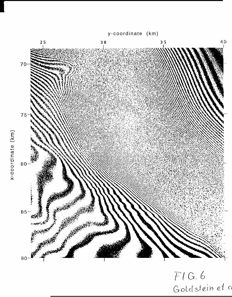
eastward into the marginal shear zone. in l~ig. 1 the fringes secm to clisappcar in the marginal

shear zones, suggest ing that the radar returns from these zones were incoherent. ] lowcvcr, an

cnlargcmcnl of

the Minnesota

par[ of the intcrfcrogram, given in l~ig, 6, shows that in the marginal area near

Glacier, w}~cre the marginal frin.gcs arc scmcwhat wiclcr than elsewhere,

cohcrcncc is not lost and cxtrcmcly fine fringes can bc detected and counted clear throug}l the

Z.OIIC. ] ~ron~ the assumed zero point Up to {Ilc fringe peak at (x,z) = (38 X) a tofal of 147 fringes

is ccmntcd. lkom tbc peak tbc fringes can bc c.ountcd downward by two diffcrmt paths, roughly

along y =20 km ancl y== 30 km in ]~ig. 1, to points in tbc grounded 7011c: at (x,y) = (2.0,2,5) the

downward count is 60 fringes by both paths, giving a net upward fringe count of 147--60=87

relative to the zero. The corresponding flow velocity at (x,y)=(12,25) is 87 X1.2 cm d-l== 381

m a- ‘. (In principle there is a correction duc to the fact that 0 varies along the traverse where

the fringes were countcci, but the correction proves to bc small,)

An alternative mctbod for identifying the Z.cro-velocity fringe makes usc of tbc curving

flow of the Minnesota Glacier that is indicated by the curving flow bands in l:ig. 4: where the

curving bancls have a “horimntal” tangent in 1 ‘ig. 4, the flow is pcrpcnclicu]ar to Ihc raclar beam

anti the line-of-sight vclocit y component is O. ‘1’his criterion, applied to the flow bands ancl

ciO1/l)STINN 111’ AI.. -9

fringes near (x,-y) =(69,21 ), selects a zero fringe that ciiffers by about 3/4 of a fringe from the

onc chosen at (x,y) == (34 ,5).

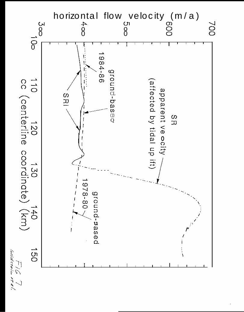
IIy fringe counting as dcscribcci above (with correction for variation of 0), the apparent

flow velocity was determined along a near-ccntcrlinc longitudinal profile starling at (x,y) == (O, 14)

and shown by the longitudinal line in IFig. 5. ‘1’hc results arc given in }~ig. 7 (solid ant] clot-dash

curve), where they are compared with ground-based velocity mcasurmcnts along the same

profile (dashecl and dottecl curves) (10). in 1 jig. 7 the velocity data arc plotted against the

longitudinal ccntcrlinc coordinate (cc, in km) used by (10); cc is 100 at the upstream cncl of the

longitudinal profile in }~ig. 7. l~rom cc 100 to about 124 the agrccmcnt bet wecn the S1{1 velocity

mcasurcmcnts and the ground truth is rather good, although the SRI velocities arc generally low

by about 10 m a- 1 (2%) in relation to the ground-based velocities, which were measurecl in

1978-80 ancl 1984-86. This discrepancy could arise if the ice motion at the assumed fringe zero

point was not zero, or it might bc due to a secular dccrcasc in flow velocities from the epoch

of the grouncl surveys to 1992. ‘1’hc small increase in velocity from 1978-80 to 1984-86

indicated by the ground data is statistically of only marginal significance according to (10).

A velocity profile across the grounciecl ice stream at x = O, based on the fringe pattern in

1 jig. 1, is given in l~ig. 8 and compared with ground-basccl velocities along nearby transverse

line l) of (10), at cc 100. The wiclc central bancl of nearly constant velocity is sharp]y

clistinguishcd from the narrow marginal z.ones of high shear, about 4 km wide. A similar pattern

is shown by ICC Stream 11 except that its central band contains pronounced velocity variations,

which appear to bc rclatccl to basal topography (2). ]:ig. 8 suggcsls, like IJig. 7, that there has

been a secular ciccrcase in flow velocity by about 10 m y- 1 from 1978-80 to 1992.

,

CiOI,IX1’l~IN lrI’ AI.. - 10

‘J’idal Motion and Grounding 1,inc

IIownsmam from cc 128 in 1 ‘ig. 7 the apparent horimntal velocity detcminccl from S1{1

as ciescribcd above shows a large upswing to a much higher ICVC1 that continues to the end of

the ccntcrlinc longitudinal profile at cc 145, Fig. 1 shows that the high

cxtcncl continuously with modest dccrcase along a broad central band

apparent velocities

from the peak at

(x,y) = (38,25) for some 50 km southward and somewhat eastward to the eclgc of the image and

CIoubtlcss bcyoncl . ‘J’hcsc high apparent velocities arc clue to vcrlical motions where the ice

stream is afloat and moves vcr[ically with the ocean tide. The tidal motions contribute strongly

to the line-of-sight displacements detected by SRI, because the line of sight is inclined only

O =230 from vertical. I lcnce when tidal motions are involved the SRT results cannot be

intcrprctecl in terms of a hori7jontal icc flow velocity alone. I;or this reason the par[ of the SRI

curve beyond cc 128 in l~ig. 7 is shown with a dash-dot line to distinguish it from the curve

upslrcam from cc 128 where the icc is grounded and the horizontal velocity interpretation is

most] y valid, (’1’hc verlical component of flow velocity for the grounded ice stream has a

gcncrall y negligible effect except as noted in the next sect ion.)

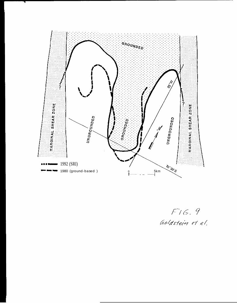
‘1’hc heavy dashed curve in liig. 9 is the grounding line as mapped on the ground (12),

ancl the heavy solid curve, drawn from l~ig. 5, is the sharp ccigc of the ca,-7-lm~-wide “tongue”

of broad, widely spaced fringes that runs southward from about x== 6 to a tip at abou[

(x,y) = (22,24). outside of this “tongue” the fringe count rises rapiclly, corresponding to the

upswing of the dash-dot curve beyond cc 128 in 1 Jig. 7, The fairly good agrccmcnt between the

dashccl and solid curves in 1 ~ig. 9 supports intcrprctat ion of the edge of the “tongue” as the

grounding line.

~OIJ)S’1’I{lN 1;’1’ Al,. - ] 1

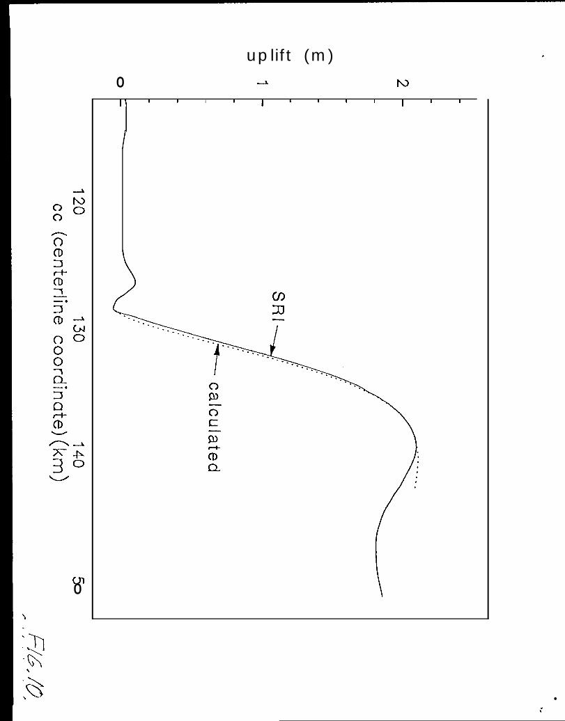
in order to evaluate ticlal motion as lhc cause of the fringe pattern outside Of’ the “longuc”

wc interpret the S1{1 velocity curve in l~ig. 7 as follows. Wc subtract from the solid and dash-

clot Gurvc in l~ig. 7 a horizontal velocity component given by tbc ground-based measurements

(dashed curve) reduced cvcrywhcrc by 8 m a- 1 so as to match generally the SRI results for the

grounded icc stream (solid curve). I’hc remainder (after the subtraction) is rcconvcr{ed to fringe

counts and then rcprojcctcd to the equivalent vertical displacement that would produce these

frin~c counts. “1’hc result is p]ot[cd as the solid curve in Fig. 10. It shows that a tidal uplift of

about 2 m between the first and second radar observations would account for the magnitude of

the rise in fringe count beyond the grounding line. Since the observed tidal ampli(udcs are of

orclcr 2 or 3 m, a tidal uplift of this magnitude bctwccn the two observations is quite possible

if the phasing of the tides was right, This can be chcckcd bccausc the Fourier con~poncnts for

the observed tide near the ungrounded Rut ford ICC Stream have been evaluated (12,24). on this

basis, C.S.M. Doakc (personal col~ll~~~lllicatio~l) has kindly calculated by l;ouricr synthesis the

ticlal level at the two observation times and finds that bctwccn the first ancl second observations

there was a tidal rise of 2.1 ~ 0.2 m, which corresponds WCI1 with the peak of the solid curve

in l;ig. 10.

“J’hc distance scale of about 10 km over which the tidal uplift incrcascs from O at the

grounding line to 2 m at the uplift peak in l~ig. 10 is rcasonab]e, as is seen by calculating from

the theory of icc shelf tidal flcxurc the cxpcctcd shape of the uplift curve. Accorcling to

standard bending-elastic-beam model of tidal flcxurc (24) the ticlal uplift curve Az(x) for

ungrounded part of the icc stream has the form

the

the

.

(2.)

] ]cI12 Az(x) is the change in elevation of’ the icc s~lrfacc at ~ whcll the far-field tidal rise fronl

observation 1 to observation 2 is Azm; x is clistancc downstream from the grounding line, and

~ is a parameter that dcpcncls on the ice thickness and elastic modulus. I’he clotted curve in IJig.

10 is calculated from cqn. (5) with Azm =2.07 m and with (3=0.26 km- 1, close to the preferred

mode] value of Smith (24) for the Rut ford ICC Stream (~=- 0.25 km- 1). ‘1’hc origin for x, where

AZ= O, is taken at cc 128 (2.5), ‘1’hc Sood agrccmcnt of the observed and calculated curves in

I Jig. 10 supporls the tidal uplitl interpretation (26).

‘J’he progressive decrease in fringe count along the central band of broad fringes that

extends downstream from the fringe peak at (x,y) == (38 ,25) is probably due mainly to

downstream dccrcasc in the flow velocity of the ice stream, cent inuing downstream the trend

seen over the interval cc 114-146 in the ground-based velocities (liig. 7, dashed curve).

lntcrprctcd in this way, the fringe pattern indicates a flow velocity of about 255 m a- 1 where

the central band exits from the image at (x,y) =70,50.

Where the Minnesota Glacier enters the icc stream, near (x,y) =’ (75 ,25) (1 ~i.g. 1), the

closely-spamd fringes in the marginal shear zone of the icc stream are “pushed” inward into the

icc stream. l)art of this feature is seen in enlarged detail in l~ig. 6, The “push-in” extends into

the central band of broad fringes near (x,y) = (64,36). ‘1’his feature reflects some combination

of rcduccd flow velocity and/or rcduccd tidal uplift in the area where the glacier enters the ice

stream. 1 tither or both effects could result from grounding or partial grounding of the icc stream

in this area, duc to ice thickening that results from inflow of the tributary glacier. l>oakc ct al.

(9) have identified the area of the “push-in” as onc of a number of locally grounded areas

?

(k)] J)STIHN 1;1’ Al,. - ] ~

locatccl by radio-echo sounding clownstrcam from the main grounding line. The curious

“IM3I1ow” in the fringe pattcm near (x,y) =- (44,38) appears to correspond to the upstream tip of

anotbcr such grounded area.

‘I’}~ccol~lparisol~ iIII~ig, 9bctwcc~] tl~cgrou~~dillg lit~eas i11dicatedbyl;ig. 1 (1992 data)

and the earlier (1980) ground-based determination (12) suggests some retreat of the grounding

line bctwccn 1980 and 1992, perhaps as much as a kilometer near the tip of the “tongue,” and

possibly several kilometers on the western side of l;ig. 9. IIowcver, such a conclusion is at this

stage made somewhat unccr[ain by possible uncertainty in registration bctwccn the SAR image

and the ground-based map (23), and also by tbc problematical aspects of the ground-based

determination of the grounding line, as indicated by comparing the results of (12) and (24).

\7cr[ic.a] flow componcmt of grounded ic.c

ljrom cc 124 to 129 in l~ig. 7 the SR1 velocity (solid curve) traces out a small peak at

cc 126 followed by a small minimum at cc 128, which are not seen in the grouncl-based (dashed)

curve. We interpret thcm as due to mall vertical motions of the grounded ice, which arc

rcprcscnted by the corresponding small peak and minimum in ] ~ig. 10. These features

approximatc]y bracket an ice-surface hump that is visible near lat, 78029.7 ‘S, long, 8305’ W in

1.anclsat optical images (9,10,21). Ice flow over the hump (27) results in a relatively upward

vcr[ical component of ice motion on the upstream side ancl a relatively downward component on

the downstream side, which produces the peak followed by a minimum at cc 126 and 128 in Fig.

10. l;ronl the height and horizontal dimension of the hump (20 m ancl 2 km) and the horizonta]

velocity (390 m a- 1) we can estimate the expected difference in ver[ical velocity between the

C; O1.lN’lilN 1~’1’ Al/. - 14

peak and the minimum; it is 0.2 meters in 6 clays, in rough agreement wiih the difference of

0.15 meters (in 6 days) bctwccn the obscrvc(i uplif[ values of the peak ancl minimum in IJig. JO.

l~ig. 1 shows that the peak and minimum bracket a prominent bright patch seen in l~ig.

4 near the center of the ice stream. 1.ikc the marginal shear zones, the brightness of this patch

in the SAR image is probably due to crevassing, which appears to bc causccl by flow over the

hump.

Comparison of S1{1 and imaging

‘1’hc satellite scqucntia] imaging mctlmd, which has been clcvelopcd for ice-stream flow

velocity monitoring by Bindschadler and Scambos (2), is limited by pixel-size displacement

resolution (ea. 30 m) (28), whereas the resolution of SRI is not limited by the pixel size and is

very much finer, ca. 1 cm for hori?,ontal displacements, A compensating limitation for SRI is

that interference cannot bc obtained from a pair of complex images taken more than a few days

apart in time, because ongoing changes ill the ice/snow surface at the radar wavelength scale

ultimately destroy the detailed phase cohcrencc between the two images upon which the

intcrfcrencc depends. lmagcs taken 2 years apart were used to obtain ice flow velocities by the

sequent ial imaging method (2), whereas for S1<1 we here usc a pair of complex images taken 6

days apart, in the determination of flow velocities the factor -103 in improved clisplaccmcnt

resolution by SRI is thus offset by a factor -10-2 in available elapsed time for the displacement

mcasurcmcnt. 1 lowcvcr, the ability of SRI to get results in a much shorter time and without

intcrfcrcncc from darkness or cloud cover (which bedevils optical imaging) is dccidcclly

advantageous.

surface features

Also, SR1 does not depend upon the presence and resolution of pixel-scale

such as crcvasscs or snow dunes, as the imaging mcthocl dots,

Both S]<1 and the sequential imaging method are limited to

motions unless within the image there arc fixccl bcclrock points (22)

fixccl with respect to bedrock. Bindschadlcr and Scambos (2)

&31/I) S’l’IHN li’J’ AI.. - 15

clctecting only relative ice

or icc features that remain

found that broad, gentle

topographic undulations, made visible in optical (Ixmdsat) images by faint sun shadowing or

scat tcring-angle effects, remained fixed in position relative to bcclrock below and coulci bc used

as a “surrogate bedrock reference” to obtain absolute flow velocities by sequential imaging.

Surprisingly they repor[ 41 pixel (528 m) precision in locating these undulations in the images,

even though the undulation wavelengths are much longer, >1 km (2). Some of the un(iulations

appear similar to the hump on Rut ford Ice Stream noted in the last section. 1 lowcvcr, for SRI

there is no counterpart to the undulation bedrock reference. ‘1’o obtain an approximation to

abso]utc flow velocities in an ice stream by S1<1 one is therefore dcpcncicnt upon assuming a

rcfcrencc point of O or small velocity outside the icc stream (29). This approach is also

cicpcndcnt on resolution of the closely spaced fringes clear through the marginal shear zone,

which is difficult, as noted earlier. ‘1’his approach can bc used to monitor the icc streams for

substantial changes of flow without danger of more than a small error from change in ice motion

at the rcfcrcncc point bccausc the flow velocities outside the ice streams are comparatively so

small (2,6)0

‘1’hc limitation of S1<1 to dctecticm of motion only in the line-of-sight direction of the

radar beam means that only onc component of the horizontal flow can bc mcasurcci from an

inla~c pair, whereas the imaging method obtains the full horizontal velocity. “1’hc limitation

could bc ovcrcomc by a second set of S1{1 data with a roughly perpendicular line of sight, but

this may or may not bc obtainab]c, ctcpcnding on the orbital inclination of the satellite and the

latitude of the target icc stream. 1 lowcvcr, because the ice stream motions ancl the motion

4

CXMJN’rJ;lN }YJ’ AI.. -16

semitivity of S1<1 are so large, the measurement of one component within, say, 60° of the flow

direct ion would bc sufficient for monitoring ice-stream flow changes.

S1<1 is scnsi[ivc to vertical motions, whereas the imaging method is not, ‘J’hLJs SRI can

detect tidal motions and thereby locate grounding lines, as shown above, while imaging cannot.

S1{1 monitoring of changes in grounding-line position from one intcrfcrogram to another is

probably not limited by the accuracy of grounding-line location in the fringe pattern but rather

by the registry of the interfcrograms in relation to fixed bedrock. Analogous] y to what can be

done will] opt ical images as noted above (2), for intcrfcrogram registry a “surrogate bedrock

rcfcrcncc” may be provided by features in the

in the last section or by the small maxima and

SAR image such as the bright patch mentioned

minima in vertical motion associatcci with flow

over humps in the ice surface topography, an example of which was discussed in the last section,

Conclusions

Satellite radar intcrferomctl<y (S1{1) is capable of observing the hori7,0ntal flow velocities

in grounded ice sheets and ice streams at a resolution level of about 1 m a- 1, which is in the

lower part of the range of typical ice-sheet motions S 10 m a- 1, and represents a very sensitive

detection lcvc] for the flow of Antarctic ice streams (-400 m a’ ~). Although only relative

velocity is directly measured, absolute velocity can be obtained if the relative velocities arc

rcfcrcncccl to a slow] y moving point outside the ice stream, This allows ongoing monitoring of

the ice streams for changes in flow at roughly the 2% level, the main uncertainty being not in

the S1<1 measurement but in the possible change in motion of the slow moving reference point.

Results arc obtainable in about a week (not counting data distribution and processing time).

Grounding line position can bc monitored to an accuracy of about 0.5 km, if successive S1<1

.

~[)1 JN’lHN 1;1’ Al., - 1 7

intcrfcrograms arc corcgisterccl by means of features in the SAR images or in the fringe patterns

that can bc recognized to stay fixed in relation to bcdroctc, a corcgistration tcchniquc analogous

for radar to onc that works for optical images (2). I’hc SR1 method is a significant acldition to

the satellite sequential imaging method (2) in monitoring the ice s[rcams for current changes that

may result from climatic change or internal instability. Changes in the Rutford ICC Stream arc

alrcacly detected, albeit marginally, by comparing S1<1 results with earlier ground-based

observations.

ltcfcrcmcs and noks

1. J. Ocrlcmans, C,J, van dcr Veen, lids., ICC Shee(s and Climate (Reidc], Dordrecht

1984); National Rcsearcb Council Acl 1 IOC Committee on the Relat ion bctwccn 1,and ICC

and Sca 1 Evel, Glaciers, ICC Sheds, and L%?~ I.w?l: ]i~’jcci of a COz-Induced Climdic

Change (National Academy Press, Washington, lIC, 1985); R.]). Alley, lj~isodm 13,

231 (1990); R,A. Warrick, J. Ocrlemans, in Climate Change: l~le IPCC Scienfl~c

Assessment, J .T, 1 loughton, G.J. Jenkins, J ,J. }iphraums, }kls. (Cambriclgc lJniv, l’ress,

1990); M.1~. Meier, Ab[we 343, 115 (1990); 1<.11. Alley, l.hl. Whillans, Science 254,

959 (1991); C.S. ].inglc, 1).11. Schilling, J.].. 1 ;astootc, W .S.11. l’atcrson, ‘1’.J. Brown,

J, GcojI}Iys. Ms. 96, 6849 (1991); T.J. 1 lughcs, I’okwogeogr., I’alaeoclimtol,

l’alaeoecol. (Global and Planetary Change Section) 97, 203 (1992); l). Sugden, Nature

359, 775 (1992); S.S, Jacobs, Nature 360, 29 (1992).

2. R.A. IIindschac]lcr, ‘J’.A. Scambos, Scimce 252, 242 (1991).

7. . 1).1{. MacAycal, Nature 3S9, 29 (1992).

4,

5. .

6,

7.

9.

10.

11.

12.

13,

~O1,l)S’1’}llN 1;1’ Al,. - 18

11.J. ~,Wa]]y, A,C. ]h3111W, J.A. Major, R.A. Bindschacller, J.G. Marsh, Science 246,

1587 (1989); C.J, van clcr Vccn, Rm. Gcophys. 29, 433 (1991).

1<.11. Thomas, J. Gluciol. 24, 167 (1979).

C,]<. IIentlcy, J. Geophys. Res, 92, 8843 (1987); 1.M. Whillans, J. Bolzan, S. Shabtaic,

J. (kof)hys. A’c?s. 92, 8895 (1 987).

T.J. IIughes, Rev, Geo/~hys. S@cc Phys. 1S, 44 (1977); J. Wcerhnan, G .1;, Birchficlcl,

A n n . Glaciol. 3, 316 (1982); C.S. 1.ingle, “1’.J. l~rowJl, ]n IIynmics of the West

Anfarcfic Ice Shed, C.J. van dcr Vecn, J. ocrlcmans, lkls, (11. Reidel, Norwell, MA

1987) p,279; C.J. van dcr Vccn, ibid., p. 8.

1{.11. Alley, D.D. IIlankcnship, S.T. Rooney, C.]<. Bentley, J. Gkmiol. 35, 130 (1989);

11. l{ngclhardt, N. ]]umphrcy, 11. Kamb, M. l;ahncstock, Science 248, 57 (1990); 1<.13.

Alley, l@isodes 13, 235 (1990); 13. Kamb, J. Geojjhys. Res. 96, 16,585 (1991).

C.S.M, Doakc, R.M. Frolich, 11.1<. Mantripp, A.M. Smith, I>,G. Vaughan, J. Geop}lys.

RN. 92, 895] (1987).

R.M, ljrolich, IJ.G. Vaughan, C.S.M, ]Make, Ann. Ghciol. 12, 51, especially lligs, 6

ancl 7 (1989).

S.N. Stephenson, C.S,M. IIoalcc, Ann. Ghciol. 3, 295 (1982).

S.N. Stephenson, Ann. Gkmiol. 5, 165 (1984).

The basic method, but directed toward the detection of verlical displacements, was

introduced by A .K. Gabriel, R.M. Goldstein, 11 .A. Y,cblccr, J, Ckophys. Res. 94, 9183

(1 989); a version of the method for measuring horizontal flow in ocean currents was

clcscrihcd by R.M. Go]dstcin, 11 .A. Zcbker, Nature 328, 707 (1987) ant] by R.M.

Goldstein, ‘l’.l). ]Iarnctt, H .A. Zcblcer, Science 246, 1282 (1989).

.

GO1/lXTIHN IY1’ Al,. - ] 9

14. R.];, Crippcn, l$~i.rodes 15, 56 (1992).

15, We start from an approximate registry based on spacecraft orbit and image parameters.

l~or a given positioning of the first image in relation to the second, the phase at each

pixel in a test square (16x 16) in the first image is comparecl with the phase at the

corresponding pixel in the second, and the phase difference is cohcrentl y averagcxi over

tbc square by means of a discrctc two dimensional Fcmrier transfom, giving a

correlation measure. This proccdurc is repeated with the second image shifted by a

certain number of pixels relative to the first; 81 relative shifts, corresponding to shifts

to pixels in a 9X9 square, are tested in this way. If a distinct maximum in the

correlation measure is found within the 9X9 square, the maximum point is the local

registry position for the two images. ‘1’he procedure is repeated for a number of 16X 16

squares distributed across the image. in calculating the interferograms the registry

position is taken to vary across the image in accordance with the smoothed results of the

above registry search, allowing also for a discontinuity in registry position between the

ice stream and the area outside of the ice stream. ‘1’hc variation is slight, 1 pixel spacing

or lCSS, but it has a significant effect on fringe qualily.

16, 1 iach original high-resolution complex image data set supplied by the 1 iuropcan Space

Agency consists of a 2500 x 12288 array of complex numbers giving pixel amplitude and

phase, 2500 rows in the range direction (bot[om to top in l:ig. 1 ) and 12288 in the cross-

range direction (right to left). We average the pixel complex numbers by groups of 4

in the range clirect ion ancl by groups of ] 2 in the cross-range clirection, condensing the

data set to a 62.5X 102.4 array, in which phase noise has been greatly clecreascd by the

averaging. 1 iach original data set proccssccl as just described covers half of the complete

17.

18.

19.

20.

21.

22.

@31 ,IX”l’IHN 1;1’ AI,. -20

radar image, either the near-range or far-range half; the near and far halves arc combined

to form the full interfcrogram, 1 ?or the result in l:ig. 1, the pixel size on the ground is

80 m (on average) in range by 48 m in cross range, and the dimensions of the area

imaged is 100 km in range by 49 km in cross range.

If the spacecraft orbits on which positions 1 and 2 lie are not exactly parallel (as is the

case for liig. 1), J] ancl V will vary slightly across the image (right to left in I Jig, 1) and

the correction ~~1 --- ~)~ varies accordingly,

l:ig. 3 is for a “flat earth” approximation in which O at the scattering site is the same as

O at the spacecraft position.

‘1’hc SA1{ image in Fig. 4 is unconventional to the extent that in the procedure for

averaging over adjacent pixels to suppress noise, as in note (16), the complex-image

values were averaged before extracting the signal amplitude, whereas for a conventional

SAR image the individual pixel amplitudes arc firsl extracted and then averaged. The

former procedure is bct[cr for bringing out weak cictails in the image.

K. Ii. ]<OSC, J. Glmiol. 24 (90), 63 (1 979).

lJ, S. Geological Survey and British Antarctic Survey, h’ford Ice Sfrean?, Marcfica,

Satellite lmagc Map (1 :250,000) (1989).

‘1’hc l~lowcrs I lills arc bedrock (with a discontinuous veneer of snow and ice) and should

in principle provide reference points of O velocity, but their fringe pattern is so

complicated that wc cannot pick a O-velocity fringe there. l’his may imply a general

limitation on using bedrock points such as nunataks to provide the reference for absolute

velocities in the SRl method.

Ciol.lISTl{lN lVI’ Al. -21

23, ‘J’hc solid and clashed curves in l~ig, 9 arc positioned in relation to the indicated latitude

and longitude lines as follows. l;or the solid curve, the intcrfcrogram in l~ig. 5 was

resealed to the scale of the satellite image map (21) on the basis of image parameters

furnished by MA, and a transparency of the in~agc was registered to the map by

registering the icc stream margins and the Hewers 1 lills; the latitude and longitude lines

from the map were then tramferrcd to the image, on which the grounding line was drawn

cm the basis of the fringe pat [cm. For the clashed curve, the longitude and latitude lines

in 1 rig. 2 of (12) were transferred to I Jig. 5 of (12) by using as a reference the frame of

l~ig, 5 that is shown in l~ig. 2. of (12); af[cr resealing, the grounding line in liig. 5 of

(12) coulcl bc positioned in relation to the solid curve in our Fig. 9 by registering the

]atitudc and longitude ]incs,

24. A.M. Smith, J, Glmiol. 37, 51 (1991).

25, This is the appropriate choice of origin because dAz/G?x = O on the observed (solid) curve

there, which is what the model (19) assumes. IIccausc the model has Az = O there, the

uplift values on the calculated (dotted) curve arc obtained by adding Az(x) from eqn. (5)

to the observed uplift value ( –0.05 m) at cc 128.

26. Very close agreement is not cxpcctcd, because the model assumes a two-dimensional

flcxurc geometry whereas the actual geometry is decidedly three-dimensional, with the

“tongue” of grounded icc surrounded on three sides by ticlal Up]if[ (];ig. 1).

27. Strictly, instead of “flow over the hump” wc should say “flow over bedrock features that

are responsible for the hump” or “flow following the curve(l surface of the hump.”

.

~01.INl’lHN IJ3’ AI,. -22

28, ]Iinclschadlcr and Scambos (2) report achieving sub-pixel resolution by a cross-correlation

mctlmcl, and Crippcn (14) cites examples of O. OS-pixel precision in sequential imaging

applied to tectonic deformation, but these resolutions are still far inferior to SRI.

29. This assumption can be avoided where flow transverse to tbc line of sight occurs within

tbe image, as in the Minnesota Glacier discussed earlier.

Figure Chptions

~OIJ)S’1’lLIN Ji’1’ A I , . - 2 3

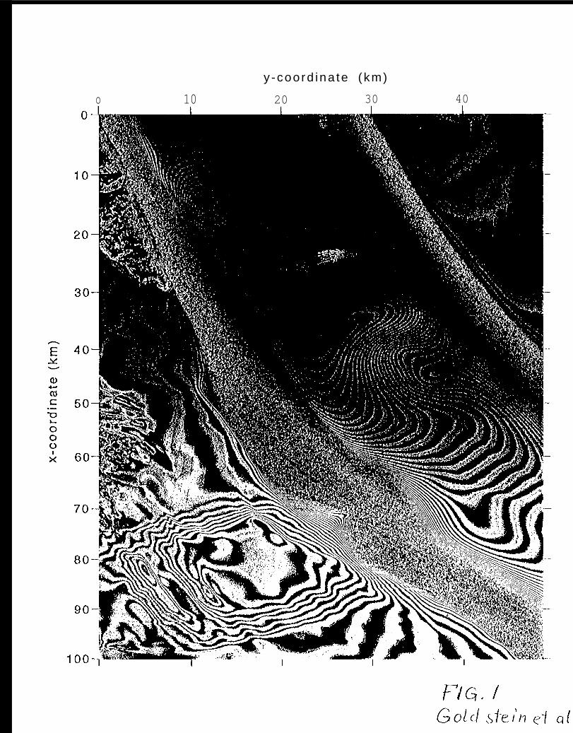
1 ~ig. 1. Radar intcrfcrogram of an area that includes a portion of the Rutford Ice Stream,

Antarctica, produced by Satellite Raclar lntcrferomctry (SRI) as described in the text. ‘l’he radar

line-of-sight direction (“range direction”) is up. The color fringes show the phase shift of the

radar return, which is duc to movement of the ice surface relative to the spacecraft during the

6-day period bctwccn two radar observations of the same scene. Phase shift modulo 360° is

coded in 16 spectral color steps covering the range from 0° to 360°. ‘lshc distance scales in the

range direct ion (up-down) and cross-range direct ion (left -right) are different, as shown by the

ticks along the margins indicating x and y coordinates in km. Supcrhnposed on the phase-shift

intcrfcrogram is a radar amplitude image (conventional SAR image) of the same area, in shades

of gray, I/or further information scc l~igs. 4 and 5.

I Jig. 2. lnterfcrcncc geometry for radar waves emanating from and returning to the radar

satellite at two nearby positions, labeled 1 ancl 2. l)ositions 1 and 2 are occupied momentarily

by the satellite at different times and lic on different local orbital paths, which arc perpendicular

to the plane of the paper. The distance between positions 1 and 2 is designated in terms of its

horizontal component 11 and vcrlical component V, The outgoing and returning (scattered) radar

waves transmitted and reccivcd at each of the two spacecraft positions arc represented by

o~ltgoillg/returl~it]g rays inclined at angle O to the vertical. The scattering point on the ground

is far away (-850 km), so the rays are drawn parallel. If the scattering point remains fixecl in

position, the plane wave returning to position 1 will lead the wave returning to position 2 by

twice the distance s indicated

by C#J~ –~q ==(2s/h)03600.

Go] .l)S’l”I:lN lrl’ A1.. -24

n the drawing, hence wave 2 is phase shiflccl relat ivc to wave 1

Fig. 3. Geometry of the ground-elevation effect on SRI. I’he plane of the diagram is

the same as 1 ~ig. 4, but the scale here is much compressed: the elevation of the spacecraft is

-800 km, whereas 13 and V in l~ig. 4 arc -10 m. IIcncc 1 ancl 2 are shown here as a single

point, labeled “spacecraft positions 1 and 2.” The radar ray path for scattering from the top of

a peak (point T) at elevation z above the datum is compared with the ray path that would be

followed if there were no mountain and the scattering were from a point Bon the datum directly

below T. Since z is small compared to the slant range P (-850 kn~), t~~e awzle Ad can be

treated as infinitesimal.

liig, 4. Conventional SAR in~agc (19) of the same area as liig. 1. Brighter areas

represent greater strength of the radar return. ‘1’hc Rutford ICC Stream is the wide dark band

with bright margins that enters the frame at the top, toward the left side, ancl extends

southeast ward, exit ing out the lower half of the cast side of the frame.

ljig. 5. I~ringe pattern from the inlcrferogram of l~ig. 1. Pixels for which the phase shift

is in the range 2250-2360 (color red in l;ig. 1) are here markccl with a black dot. “1’hc image

area is the same as in l~ig. 1, cxccpt for omission here of an 11-km-wide strip at the bottom.

‘1’hc x,y coordinate systcm, in km, shows the dimensional scale and is used in the text to locate

points in the image. The image distortion in l;ig. 1 duc to nonlinearity of the x scale and

inequality of the x and y scales is here removed. 1 xititudc and longitude are shown by labeled

,

C; O1.]mli]N 1~1’ Al,. -25

crosses. The longitudinal

along which flow velocity

line running somewhat east of south from (.x,y) u (O, 14) is a profile

and tidal uplift data are given in l~igs. 7 and 10. Within the area of

the l~lowcrs 1 lills (upper left, west of the ice stream), radar amplitude information is included

in order to improve the visibility of the hills for registry with other images such as lmdsat.

1 jig. 6. llnlargement of a portion of l~ig. 1 in the area where the Minnesota Glacier feeds

into the Rutford Ice Stream. ‘1’he radar amplitude (SAR) image is here omitted, so that only the

phase shift between the two complex images is portrayed. ‘1’hc enlarged area is bounded by x

and y coordinates as indicated, l~or greater spatial resolution of the fringes, the data averaging

proccdurc (16) is here modified by averaging over only 4 pixels in the cross-range direction and

eliminating averaging in the range direction, giving a pixel size 16 m X 20 m.

l;ig. 7. ICC stream flow velocities along the longitudinal profile marked in l:ig. S. “J’he

abscissa is the longitudinal ccntcr]inc coordinate (cc, in km) of (10), with origin 100 km

upstream from the start of the profile shown here. cc 100 corresponds to x ==0 in I Jig. 5, The

curve labeled SRI is obtained from the SRI data in l~ig. 1 under the assumption that the phase

shift results from horizontal mot ion in the direction of ice-stream flow (see text). This

assumption holds for most of the solid part of the curve, but not for the dash-dot part, which is

greatly affected by vertical (tidal) motions and therefore represents unreal horizontal velocities.

The dashed and dotted curves arc ground-based velocity measurements made in 1978-80 and

1984-86 rcspcctivcly (10).

~OIJ)ST1;IN In’ A l . . - 2 6

l~ig. 8, Transverse profile of flow velocity at x=-O from SRI (solid curve) and from

ground observations (dashed curve) ontransversc profile D of (10), which is a transverse line

passing approximately through (x,y)=(3,7). l~ccausc the transverse direction is24° askew to

the x= O profile line, the transverse coordinate for plotting the profile-l) velocities has been scale

up by (COS 240, -1 so that the edges of the icc stream in the two

y= 32. In the marginal shear zones, where the fringes are too

velocity curve is interpolated by dash-dot lines to velocity values

near-zero velocity is assumed, A similar interpolation would

profiles match, at y== 1 and

narfow to resolve, the S}<1

just at the margin, where a

apply to the ground-based

measurements, which do not extend into the marginal shear zones.

Fig. 9. Map of the grounding line of the Rutford Ice Stream: solid curve: grounding

Iinc as obtained from SR1 in 1992 (Figs. 1 and 5); dashed curve: grounding line as found from

ground observations in 1980 (12,23). The area of currently grounded ice is lightly patterned,

and the marginal shear zones arc more heavily path.med. Icc flow is from top to bottom.

l;ig. 10, Tidal uplift of the Rutford Ice Stream. The solid curve is the uplift observed

by SRI (l~ig. 1) on the basis described in the text. The tidal uplift starts at the grounding line

at cc 128 and grows rapidly downstream. The dotted line is the theoretical tidal uplift calculated

from cqn. (2) with AZm==2,07 m, f3==0.26 km-1, and with x= O at cc 128, The small observed

peak at cc 126 and trough at cc 128 are uplift features related to icc flow over a topographic

hump as discussed in the text.

y -coord ina te ( km)

o 10 20 30 400-

lo-

20-

30-

40-

50-

60-

70-

80-

90-

1oo-

F-/G< fGoh Lsi-dIq <-t (i

S p a c e c r a f tPosition 2

// A%’ “

\f

S p a c e c r a f t \ HPosition 1

:073

radar rays returningfrom ground surface

at great distance

F/L’Z’, 2

SpacecraftPosit ions1 and 2

e

\P\

ray path to /datum below peak

Horizontal Datum PlaneB

F-/&, 3

n

y-coord inate (km)

o 10 20 30 400

10

20

30

40

50

60

70

80

!30-. . .

.“: :: . ..-’.. ‘+ -

100--[-J=”” ““< I

,,

y–coordinate (km)

o 10 2 0 3 0 4 0 5 00

1 0

20

30

6 0

7 0

8 0

9 0) -. / c

y -coord ina te ( km)

2 5 3 0 3 5 40

70-

75-

80-

85-

90-

0

(’D

o0O-A

A

--PXo

3

(Ao0

-Po0

horizontal flow velocity (m/a)mo0

mo0

1 I I 1\i

1 1 I I I 1 I I I I I I I I

mzcsCL

&@u)CDQ

I&I*

/t-..I -. --- - - - -

-.=-. -.=

I u

(/)3J

-------- /. . .

-. \.

I

;

00-.

G

.)

/“./

/“/“

/

i

1 1 1 I I I 1 1 1 I 1 I 1 I I 1 I 1 1

.\

,.

.

1992 (SRI) / \1980 (ground-based ) o 5km

\

‘W@F---- - – —-{

.

0-l0

\

0

uplift (m)A N

l\ I I I I I 1 I I I I I I

/

\

. .

\

.,.

●

✚