Old, frail, and uninsured: Accounting for features of theU.S. long-term care insurance market ∗

R. Anton BraunFederal Reserve Bank of Atlanta

r.anton.braun@gmail.com

Karen A. KopeckyFederal Reserve Bank of Atlantakaren.kopecky@atl.frb.org

Tatyana KoreshkovaConcordia University and CIREQ

tatyana.koreshkova@concordia.ca

January 2019

Abstract

Half of U.S. 50-year-olds will experience a nursing home stay before they die, and one inten will incur out-of-pocket long-term care expenses in excess of $200,000. Surprisingly,only about 10% of individuals over age 62 have private long-term care insurance (LTCI)and LTCI takeup rates are low at all wealth levels. We analyze the contributionsof Medicaid, administrative costs, and asymmetric information about nursing homeentry risk to low LTCI takeup rates in a quantitative equilibrium contracting model.As in practice, the insurer in the model assigns individuals to risk groups based onnoisy indicators of their nursing home entry risk. All individuals in frail and/or lowincome risk groups are denied coverage because the cost of insuring any individual inthese groups exceeds that individual’s willingness-to-pay. Individuals in insurable riskgroups are offered a menu of contracts whose terms vary across risk groups. We findthat Medicaid accounts for low LTCI takeup rates of poorer individuals. However,administrative costs and adverse selection are responsible for low takeup rates of therich. The model reproduces other empirical features of the LTCI market including thefact that owners of LTCI have about the same nursing home entry rates as non-owners.Keywords: Long-Term Care Insurance; Medicaid; Adverse Selection.JEL Classification numbers: D82, D91, E62, G22, H30, I13.

∗We thank Taylor Kelley and Jordan Herring for outstanding research assistance. We are grateful fordetailed comments from the editor, the referees and also from Joseph Briggs, Martin Eichenbaum, EricFrench, John Jones, Robert Shimer and Ariel Zetlin-Jones. We also benefited from comments received at the2015 Workshop on the Macroeconomics of Population Aging in Barcelona, Notre Dame University, the CanonInstitute for Global Studies 2015 End of Year Conference, the Keio-GRIPS Macroeconomics and PolicyWorkshop, the 2016 FRB Atlanta Workshop on Adverse Selection and Aging, the 2016 SED meetings inToulouse, the 2016 CIREQ MacroMontreal Workshop, the Michigan Retirement Research Center Workshop,

1

1 Introduction

Nursing home expense risk in the U.S. is significant. Half of U.S. 50-year-olds will experiencea nursing home stay before they die, and one in ten will incur out-of-pocket long-term care(LTC) expenses in excess of $200,000. Surprisingly, only about 10% of individuals over age62 own private long-term care insurance (LTCI). Even though takeup rates increase withwealth, they are low at all levels of the wealth distribution. In our sample of Health andRetirement Study respondents, they are under 2% for individuals in the bottom wealthquintile and 20% for individuals in the top wealth quintile.

Why are LTCI takeup rates so low? Using a quantitative equilibrium contracting model,we analyze the role of three factors. First, LTCI is costly to produce. LTC insurers facesignificant variable and fixed administrative costs. Commissions to brokers often exceedthe first year’s premium income. And insurers allocate more resources to underwriting andclaims management for LTCI as compared to other life insurance product lines. Second,individuals have private information about their nursing home entry risk.1 As a result,insurers are exposed to adverse selection. Third, Medicaid offers public assistance for nursinghome expenses to individuals who satisfy a means-test.

According to our model, the primary factors leading to low LTCI takeup rates varyacross the income distribution. In particular, Medicaid is responsible for low LTCI takeuprates among poor individuals; both Medicaid and administrative costs are important for lowtakeup rates among the middle class; and adverse selection and administrative costs accountfor low LTCI takeup rates among affluent individuals. The model also accounts for a rangeof other empirical features of this market. Notably, owners of LTCI in the model have aboutthe same nursing home entry rates as non-owners.

Our model builds in the following aspects of how underwriting works in practice. U.S.LTC insurers screen individuals in two ways. They collect information about each applicant’shealth status and finances and use it to assign the applicant to a group of people with similarnursing home entry risk. Some applicants get assigned to an uninsurable risk group and aredenied coverage. Applicants who are selected for insurance are offered a specific menu ofinsurance policies whose terms vary across risk groups.

We consider the problem of a monopolist insurer who incurs fixed and variable costs ofproviding insurance. Individuals in the model have access to public means-tested nursinghome benefits. They also have private information about nursing home entry risk. Theinsurer in our model assigns each individual to a risk group based on observable indicatorsof health status and income. As in practice, the insurer screens individuals in two ways.First, the insurer conducts risk-group selection: it decides which risk groups to insure andwhich ones to deny coverage. Second, it decides the menus of contracts for insurable riskgroups. There are two ways that an individual may end up with no insurance. He may beassigned to an uninsurable risk group or he may be assigned to an insurable risk group butdecide that none of the policies offered to his risk group are attractive to him.

FRB Chicago, FRB Minneapolis, FRB Richmond, FRB St. Louis, Carlton University, Purdue University,McGill University, University of Mannheim, and the 2018 University of Minnesota HHEI conference.

1Finkelstein and McGarry (2006) find that self-reported nursing home entry probabilities predict nursinghome entry even after controlling for observables.

2

In the model, all three factors — administrative costs, Medicaid, and variation in thedistribution of private information across risk groups — influence both risk-group selec-tion as well as pricing and coverage of contracts offered to insurable risk groups. Variableadministrative costs increase the marginal cost of offering insurance. With variable costs,coverage levels are lower and unit prices are higher relative to the optimal contracts in aworld where variable costs are zero. If variable costs are sufficiently large, all individuals insome risk groups are denied coverage. Fixed costs may also make it unprofitable to insureany individual in some risk groups, leading the insurer to deny coverage to the entire group.

The insurer also recognizes that low income individuals have low or even no willingness-to-pay for private insurance because they have a high probability of qualifying for Medicaidbenefits. As a result, the presence of Medicaid induces the insurer to deny coverage to allindividuals in low-income risk groups. Medicaid also lowers the willingness-to-pay of moreaffluent individuals because it provides free nursing home benefits in the, possibly rare, statesof the world where the individual has exhausted his personal resources. Thus, Medicaid alsoimpacts the set of contracts offered to insurable risk groups.

Absent Medicaid and administrative costs, our model is equivalent to the model of Stiglitz(1977). A sharp implication of that model is that all risk groups are insurable. This implica-tion is inconsistent with the fact that LTC insurers deny coverage to all individuals in somerisk groups. Our model accounts for this fact because we combine private information withMedicaid and administrative costs. Once either Medicaid or administrative costs are present,the distribution of private information within a risk group impacts whether or not that riskgroup is insurable. Chade and Schlee (2016) make this point in a theoretical framework withprivate information and administrative costs. We show that this same point applies whenMedicaid is present.

To assess the quantitative significance of Medicaid, administrative costs and private in-formation in accounting for low LTCI takeup rates we parametrize the model as follows. Theparameter that governs the scale of Medicaid in the model is set to reproduce U.S. benefitlevels. Administrative costs in the model are chosen to reproduce U.S. industry averagesof fixed and variable costs. The distribution of nursing home entry risk varies across riskgroups in the model. We discipline this variation by targeting the variation in mean nursinghome entry and LTCI takeup rates by frailty and income. Finally, the overall dispersion inprivately-observed nursing home entry risk is chosen to reproduce the coefficient of variationin self-reported nursing home entry probabilities for Health and Retirement Survey (HRS)respondents. These targets are estimated using HRS data.

The parametrized model reproduces a variety of non-targeted statistics. The dispersion inprivately-observed nursing home entry risk in the model is higher in frail and poor risk groups.This pattern is consistent with patterns of dispersion in self-reported nursing home entryprobabilities in the HRS data. The average extent of coverage and premia in the model is ingood accord with the data, too. Finally, the model reproduces the low correlation betweennursing home entry risk and LTCI ownership documented in Finkelstein and McGarry (2006).

Our first step in understanding the role of the three factors in accounting for low LTCItakeup rates is to ascertain the quantitative significance of the two screening devices usedby insurers: risk-group selection versus menu design for insurable risk groups. In our modelscreening is conducted almost exclusively via risk-group selection.

Next, we quantify the relative impacts of Medicaid, administrative costs and private

3

information on the extent of risk-group selection and, hence, average LTCI takeup ratesin the model. We find that removing Medicaid increases average takeup rates by 81 per-centage points and removing administrative costs increases them by 51 percentage points.Finally, eliminating private information by assuming the insurer can observe individuals’actual nursing home entry probabilities increases takeup rates by 28 percentage points.

Medicaid, administrative costs and private information each play a distinct but essentialrole in generating the pattern of low takeup rates by income and frailty in the model. Med-icaid generates low takeup rates of the poor who can easily meet its means test and, as aresult, have very low willingness-to-pay for private insurance. Both Medicaid and adminis-trative costs have a large impact on the takeup rates of middle-income individuals. However,Medicaid’s impact on more affluent individuals is small. Their low LTCI takeup rates are,instead, due to the presence of private information and administrative costs.

Our empirical results shed new light on other findings in the literature. Brown andFinkelstein (2008) consider the impact of Medicaid on the demand for LTCI in a settingwith exogenously specified insurance contracts. They find that individuals in the bottomtwo-thirds of the wealth distribution do not purchase a full insurance actuarially-fair productwhen Medicaid nursing home benefits are available. Our strategy of modeling the insurer’sproblem creates new interactions between Medicaid and private LTCI. When Medicaid ispresent, individuals prefer private insurance contracts that feature partial coverage. Sincethe insurer customizes pricing and coverage to fit the needs of each risk group, the crowdingout effect of Medicaid is much smaller in our model.

The ability of our model to generate a low correlation between LTCI ownership andprivate nursing home entry risk is of independent interest. Standard adverse selection theorypredicts a strong positive correlation between insurance ownership and private risk exposure.Empirical evidence of a low or even negative correlation in LTC and other insurance marketshas prompted a literature searching for an explanation. Finkelstein and McGarry (2006), forinstance, conclude that multiple sources of private information are required to understandthe U.S. LTCI market. We obtain this low correlation in a model with a single source ofprivate information. Because the insurer in our model engages in risk-group selection, nearlyall risk groups have the property that either both the high and the low risk types in the groupare insured or neither are insured. As a result, LTCI ownership rates are uninformative aboutnursing home entry rates.

Finally Ameriks et al. (2016) find that more affluent individuals are not interested inpurchasing the set of LTCI policies available to them in the market but would be interested inpurchasing an ideal LTCI product. They refer to their result as the LTCI puzzle. Our resultssuggest that both private information and administrative costs are important reasons for thispuzzle. When both of these mechanisms are present, our parametrized model accounts forthe low LTCI takeup rates of affluent individuals in the data. However, when either one ofthese frictions is removed from the model, most affluent individuals purchase LTCI.

The remainder of the paper is organized as follows. Section 2 provides an overview ofthe U.S. LTCI market. Section 3 presents the model. Section 4 describes identificationand parametrization of the quantitative model. Section 5 assesses the ability of the modelto reproduce non-targeted moments. Section 6 contains our main results and robustnessanalysis, and our concluding remarks are in Section 7.

4

2 The U.S. LTCI market

In the U.S., LTCI is primarily used to insure against lengthy nursing home (NH) stays. Forthis reason we focus on NH stays that exceed 100 days.2 We estimate that the lifetimeprobability of a long-term NH stay is 30% at age 50.3 On average, those who experience along-term stay spend about 3 years in a NH. According to the U.S. Department of Healthand Human Services, NH costs averaged $225 per day in a semi-private room and $253 perday in a private room in 2016. Thus, it is not unusual for lifetime NH costs to exceed$200,000.

Given the extent of NH risk in the U.S., one would expect that the private LTCI marketwould be large. But, only 10% of individuals aged 62 and older in the HRS have private LTCIand takeup rates are low at all wealth levels. In particular, they are 4.5% in wealth quintiles1–3, 14% in wealth quintile 4, and 20% in wealth quintile 5. Moreover, in 2000, private LTCIbenefits only accounted for 4% of aggregate NH expenses, while the share of out-of-pocketpayments was 37%.4 Favreault and Dey (2016) estimate that 10.6% of individuals will incurout-of-pocket LTC expenses that exceed $200,000, and Kopecky and Koreshkova (2014) findthat the risk of large out-of-pocket NH expenses is the primary driver of wealth accumulationduring retirement.

Most LTCI is purchased from agents or brokers by individuals aged 55–66 years, whilethe average age of NH entry is 83.5 At the time of applying for LTC coverage, applicants areasked detailed questions about their health status and financial situation. Some commonquestions include: Do you require human assistance to perform any of your activities of dailyliving? Are you currently receiving home health care or have you recently been in a NH?Have you ever been diagnosed with or consulted a medical professional for the following: along list of diseases that includes diabetes, memory loss, cancer, mental illness, and heartdisease? Do you currently use or need any of the following: wheelchair, walker, cane, oxygen?Do you currently receive disability benefits, social security disability benefits, or Medicaid?6

Applicants are also queried about their income and wealth and asked to explain the specificsource of resources that will be used to pay premia. Applicants are warned that premiaincreases are common and queried about their ability to cope with future premia increases.Finally, applicants are informed that, as a rule of thumb, LTCI premia should not exceed7% of their income.7

Underwriting standards are strict and denials are common. About 20% of formal appli-cants are denied coverage via underwriting according to industry surveys (see Thau et al.(2014)). However, even prior to underwriting, insurance brokers screen out applicants. Theydiscourage individuals from submitting a formal application if their responses indicate that

2Another reason we focus on NH stays is because Medicare offers universal benefits for short-termrehabilitative NH stays of up to 100 days.

3In comparison, using HRS data and a similar simulation model, Hurd et al. (2013) estimate that thelifetime probability of having any NH stay for a 50 year old ranges between 53% and 59%.

4Source: Federal Interagency Forum on Aging-Related Statistics.5Thau et al. (2014) report that only 10% of sales in 2013 were sold at work-sites.6Source: 2010 Report on the Actuarial Marketing and Legal Analyses of the Class Program.7 Source: NAIC Guidance Manual for Rating Aspects of the Long-Term Care Insurance Model Regula-

tion, March 11, 2005.

5

they have poor health or low financial resources. Using HRS data, we estimate that 36% to56% of 55–66 year olds would be denied coverage if they applied based on health underwrit-ing guidelines from Genworth and Mutual of Omaha.8,9 Denials are high even in the tophalf of the wealth distribution, ranging from 28% to 48%.

For individuals who are offered insurance, coverage is incomplete and premia are high.Insurers cap their losses by offering indemnities instead of service benefits. Brown andFinkelstein (2007) estimate that a “representative” LTCI policy in 2000 only covered about34% of expected lifetime costs. Brown and Finkelstein (2011) find that coverage has improvedin more recent years with a representative policy in 2010 covering 66% of expected lifetimecosts.10 More recently, Thau et al. (2014) report that policies that offer unlimited lifetimebenefit periods have largely disappeared from the market. Brown and Finkelstein (2007)and Brown and Finkelstein (2011) also find that individual loads, which are defined as oneminus the expected present value of benefits relative to the expected present value of premia,ranged from 0.18 to 0.51 (depending on whether or not adjustments are made for lapses) in2000 and ranged from 0.32 and 0.50 in 2010. In other words, LTCI policies are sometimestwice as expensive as actuarially-fair insurance. Loads on LTCI are high relative to loads inother insurance markets. For instance, Karaca-Mandic et al. (2011) estimate that loads inthe group medical insurance market range from 0.15 for firms with 100 employees to 0.04for firms with more than 10,000 employees, and Mitchell et al. (1999) estimate that loadsfor life annuity insurance range between 0.15 and 0.25.

2.1 Administrative costs and profitability

Even though prices are high and coverage is incomplete, insurers have found that LTCIproducts are costly products to offer and profits have been low. In order to promote sales,brokers are given a substantial commission in the year that the policy is written and smallercommissions in subsequent years. In 2000, initial commissions averaged 70% of the firstyear’s premium and, in 2014, they averaged 105%. However, total commissions over thelife of a policy have been reasonably stable. They were about 12.6% of present-value pre-mium for policies written in 2000 and 12.3% of present-value premium for policies writtenin 2014. Administrative expenses associated with underwriting and claims processing arealso significant. These expenses averaged 20% of present-value premium in 2000 and 16%of present-value premium in 2014.11 Finally, as pointed out in Cutler (1996), LTCI prod-ucts are subject to intertemporal risk. These policies pay out, on average, about 20 yearsafter they are written and, if interest rates, retention rates or claims duration vary froman insurer’s forecast, the costs of the entire pool of policies changes. Insurers are underincreasing pressure by regulators to provision for this risk by including a markup on the

8All HRS data work is done using our HRS sample. Details on our sample selection criteria are reportedin Section 2 of the appendix.

9The denial rate is 56% if we assume that all individuals who stated that they had ever been diagnosedwith any of the diseases asked about are denied coverage and 36% if we assume that none of them are deniedcoverage.

10Most of this increase in coverage is due to the fact that the representative policy in 2010 includes anescalation clause that partially insures against inflation risk.

11These figures on costs are from the Society of Actuaries as reported in Eaton (2016).

6

initial premium. The additional proceeds are held as reserves to provision against adversefuture developments in claims.

Insurers have not been able to fully pass higher costs through to consumers. Accordingto Cohen et al. (2013), most insurers have exited the market since 2003 and many insurersare experiencing losses on their LTCI product lines. New sales of LTCI in 2009 were below1990 levels and, according to Thau et al. (2014), over 66% of all new policies issued in 2013were written by the largest three companies.12

2.2 Asymmetric information and adverse selection

One contributing factor to low LTCI takeup rates pursued in this analysis is that individualshave private information about their nursing home entry risk. As a result, insurers are ex-posed to adverse selection. Actuaries are keenly aware that the high costs of offering LTCItranslate into high premia. This negatively impacts the risk composition of the pool of appli-cants, further raising the LTCI premia (see, for instance, Eaton (2016)). Academic researchhas also documented evidence of asymmetric information in the LTCI market. Finkelsteinand McGarry (2006) provide direct evidence that individuals have private information abouttheir NH entry risk and act on it. Specifically, they find that individuals’ self-assessed NHentry risk is positively correlated with both actual NH entry and LTCI ownership even aftercontrolling for characteristics observable by insurers.

Interestingly, even though Finkelstein and McGarry (2006) find evidence of private infor-mation in the LTCI market, they fail to find evidence that the market is adversely selectedbased on the positive correlation test proposed by Chiappori and Salanie (2000). When theydo not control for the insurer’s information set, they find that the correlation between LTCIownership and NH entry is negative and significant. Individuals who purchased LTCI areless likely to enter a NH as compared to those who did not purchase LTCI. When they in-clude controls for the insurer’s information set, they also find a negative, although no longerstatistically significant, correlation. Finally, when they use a restricted sample of individualswho are in the highest wealth and income quartile and are unlikely to be rejected by insurersdue to poor health, they again find a statistically significant negative correlation.

Hendren (2013) raises the possibility that Finkelstein’s and McGarry’s findings are drivenby individuals in high risk groups. Specifically, he finds that self-assessed NH entry risk ispredictive of a NH event for individuals who would likely be denied coverage by insurers.One objective of our analysis is to assess the quantitative significance of denials. Hendren’smeasure of a NH event is independent of the length of stay. Since we focus on stays that areat least 100 days, we have repeated the logit analysis of Hendren (2013) using our definitionof a NH stay and our HRS sample. We get qualitatively similar results. In particular, wefind evidence of private information at the 10-year horizon in a sample of individuals whowould likely be denied coverage by insurers.13

12The top three insurers are Genworth, Northwest and Mutual of Omaha. For informa-tion about losses on this business line see, e.g., The Insurance Journal, February 15, 2016,http://www.insurancejournal.com/news /national/2016/02/15/398645.htm or Pennsylvania InsuranceDepartment MUTA-130415826.

13See Section 2.3 of the appendix for more details.

7

2.3 Public LTCI

Public insurance is known to have important interactions with the demand for private insur-ance.14 The primary public LTC insurer is Medicaid. It is means-tested and only availableto individuals who have either low wealth and retirement income (categorically needy) orlow wealth and very high medical expenses (medically needy). Medicaid is also a secondarypayer that only offers benefits after any private LTCI benefits have been exhausted. Brownand Finkelstein (2008) find pronounced crowding-out effects of Medicaid on the demand forprivate LTCI. Specifically, they find that in the presence of Medicaid about two-thirds ofindividuals would not purchase an actuarially-fair, full-coverage, private LTCI policy.

3 Modeling the market for LTCI

In this section we start by describing a simple model. The heart of which is a variantof the model in Rothschild and Stiglitz (1976). The model consists of a single risk groupcomprised of risk-adverse individuals and a single monopolist insurer as in Stiglitz (1977).The assumption of a single insurer is a parsimonious way to capture the concentration wedocumented above in this market.15 We extend the model by adding administrative costson the insurer and Medicaid. Our modeling of administrative costs is inspired by Chadeand Schlee (2016) who conduct a theoretical analysis of administrative costs and coveragedenials in an adverse selection model with a continuum of private types. We are unawareof other work that incorporates a public means-tested insurer into an optimal contractingframework.

We use the simple model to illustrate two distinct ways to generate low LTCI takeuprates. The first way is an optimal menu in which all individuals in a risk group are deniedcoverage. The second way is an optimal menu in which some individuals in an insurable riskgroup prefer not to purchase insurance. We describe conditions under which administrativecosts, Medicaid and the distribution of private information induce coverage denials to allindividuals in a risk group. We also describe conditions under which these factors affectthe pricing and extent of coverage offered to an insurable risk group. Having made thesepoints we then explain the additional details that are needed to make the model suitable forquantitative analysis.

3.1 Optimal contracts with adverse selection and administrativecosts

Suppose that there is a continuum of individuals and that each individual has a type i ∈g, b. They each receive endowment ω but face the risk of entering a NH and incurringcosts m. The probability that an individual with type i enters a NH is θi ∈ (0, 1). A fraction

14For instance, Mahoney (2015), finds that U.S. bankruptcy laws provide implicit insurance against largehealth expense, and Fang et al. (2008) document evidence of advantageous selection in the the U.S. Medigapmarket.

15Lester et al. (2015) propose a framework with adverse selection that allows one to investigate howoptimal contracts vary with the extent of market power. However, for reasons of tractability they assumerisk neutrality and their optimal contracts are different from ours.

8

ψ ∈ (0, 1) of individuals are good risks who face a low probability θg of a NH stay. Theremaining 1 − ψ individuals are bad risks whose NH entry probability is θb > θg. Let ηdenote the fraction of individuals who enter a NH then η ≡ ψθg + (1−ψ)θb. Each individualobserves his true NH risk exposure but the insurer only knows the structure of uncertainty.A contract consists of a premium πi that the individual pays to the insurer and an indemnityιi that the insurer pays to the individual if he incurs NH costs m. A menu consists of a pairof contracts (πi, ιi), one for each private type i ∈ g, b.

The optimal menu of contracts offered by the insurer maximizes his profits subject toparticipation and incentive compatibility constraints. Our specification of the insurer’s prof-its includes two administrative costs. The first cost is a variable cost of paying claims withconstant of proportion λ− 1 ≥ 0 and the second cost is a fixed cost γ ≥ 0 of paying claims.Thus, profits are

ψπg − θg

[λιg + γI(ιg > 0)

]+ (1− ψ)

πb − θb

[λιb + γI(ιb > 0)

]. (1)

This formulation is general enough to handle the various costs incurred by insurers that wedescribed in Section 2.16 The participation and incentive compatibility constraints for eachtype are

(PCi) U(θi, πi, ιi)− U(θi, 0, 0) ≥ 0, i ∈ g, b, (2)

(ICi) U(θi, πi, ιi)− U(θi, πj, ιj) ≥ 0, i, j ∈ g, b, i 6= j, (3)

where U(θi, πi, ιi) = (1−θi)u(ω−πi)+θiu(ω−πi−m+ ιi) is the utility of an individual withNH entry probability θi who chooses contract (πi, ιi). Individuals choose the contract fromthe menu that maximizes their utility. The participation constraints ensure that each typeof individual prefers the contract designed for his type over no insurance, and the incentivecompatibility constraints ensure that each type prefers his own contract over the other typescontract.

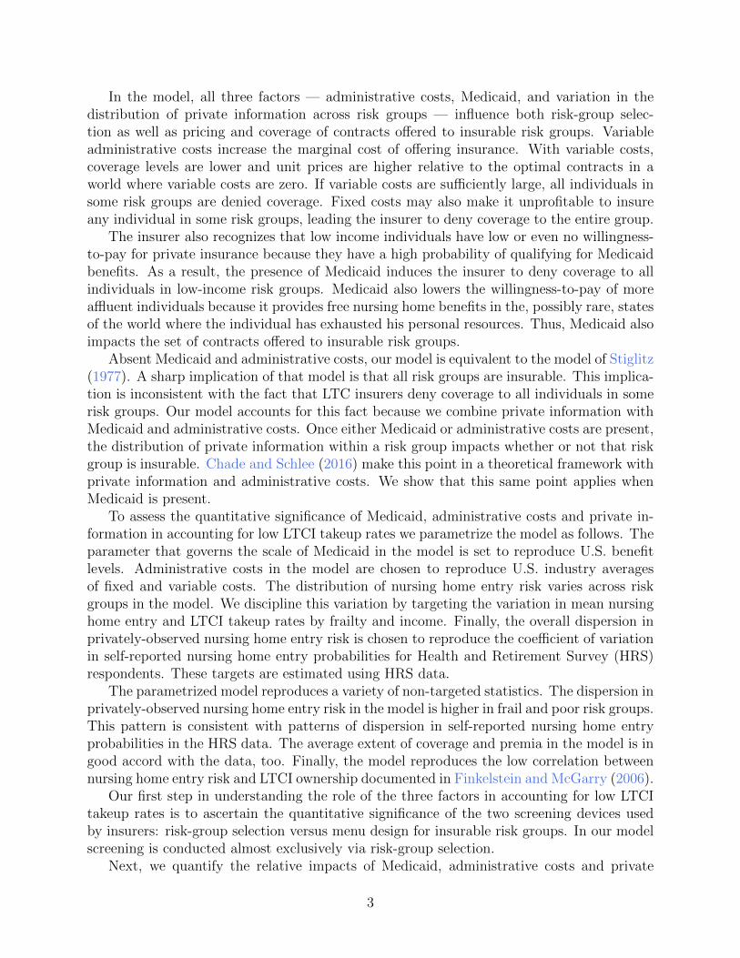
Under the optimal contracts, the participation constraint binds for the good types andthe incentive compatibility constraint binds for the bad types. Figure 1 shows various typesof optimal menus that can arise. In each case, the curve which passes through the origin(the red curve) is the binding participation constraint of the good types. The other (blue)curve, which passes through the good type’s contract, is the binding incentive compatibilityconstraint of the bad types. Each curve traces out a locus of contracts that individuals ofthe corresponding type are indifferent over taking. At each indemnity level, the slope of theindifference curve is that type’s willingness to pay for a marginal increase in coverage. Hencethe good type’s indifference curves are flatter than those for the bad type.

Figure 1a illustrates a typical optimal menu under the standard case: λ = 1 and γ =0. The menu exhibits the classic properties of an optimal menu under adverse selection.Specifically, the menu features two distinct contracts. The bad types prefer the contract atpoint B1 that features full coverage against the loss and the good types prefer the contract atpoint G1 which exhibits partial coverage, 0 ≤ ιg < m, but a smaller premium, πg < πb. Notethat pooling contracts cannot be equilibria in this setting because, starting from a pooling

16In Section 1.4 of the appendix, we show that costs that are proportional to premia such as brokerage

9

(a) Separating equilibrium withλ = 1

(b) Separating equilibrium withλ > 1

(c) Pooling equilibrium with λ >1

(d) Equilibrium with no insur-ance and λ > 1

(e) Equilibrium with only badtypes insured and λ > 1

Figure 1: An illustration of the effects of increasing the insurer’s proportional administrativecosts factor (λ) on the optimal menu. The blue (red) lines are the indifference curves of bad(good) types. The dashed blue lines are isoprofits from contracts for bad types and the reddashed lines are isoprofits from a pooling contract.

contact at a point such as G1, the insurer can always increase total profits by offering thebad types a more comprehensive contract.

In the standard case, the optimal contracts generally feature cross-subsidization fromgood to bad types. However, a separating equilibrium where the good types have a (0, 0)contract can occur if the fraction of good types, ψ, is sufficiently low and the dispersion inthe θ’s is sufficiently high. This particular type of optimal menu is important because it isthe only way for the standard model to produce a LTCI takeup that is less than one. Wewill refer to it as a choice menu. This term is used because all individuals are offered positiveinsurance, but the good-risk types choose the (0, 0) contract.

We want to emphasize that a risk group is always insurable in the standard case. Re-gardless of the distribution of private information, willingness-to-pay always weakly exceedsthe cost of insurance for the bad types. This property of the standard model is inconsistentwith the fact that LTC insurers deny coverage to some risk groups. We now turn to discusstwo distinct ways to produce coverage denials for all individuals in the risk group.

The first way is by assuming that the insurer incurs administrative costs. With non-zero

fees and pricing margins can be mapped into the variable cost term.

10

variable administrative costs, λ > 1, the optimal menu exhibits less than full insurance forboth risk types. Pooling contracts can arise and, when the costs are sufficiently large, allindividuals in the risk group may be denied coverage. The various types of optimal menusthat can arise are displayed in Figure 1. Start by by comparing Figure 1a with Figure 1bwhich shows an optimal separating menu when λ is above 1.17 Increasing λ increases theslopes of the insurer’s isoprofit lines. The insurer responds by reducing indemnities andpremia of both types, and the optimal contracts move southwestward along the individuals’indifference curves. Thus, if λ > 1, the property of the standard model — that bad types getfull insurance — no longer holds as both types are now offered contracts where indemnitiesonly partially cover NH costs.18

Since the marginal costs of paying out claims to the bad type are higher than to the goodtype, when λ increases, the contracts also get closer together and a single (pooling) contractmay arise. Figure 1c depicts such a case where both types get the same nonzero contract.Once a pooling contract occurs, the equilibrium under any larger values of λ will also involvepooling. However, the pooling contract will be lower down on the good types’ indifferencecurve and feature less coverage, lower premia, and lower profits. If λ is sufficiently largethen no profitable nonzero pooling contract will exist. Figure 1d illustrates this case of anuninsurable risk group. The optimal menu consists of a pooling (0, 0) contract, and theLTCI takeup rate is zero.19 Note that, as in the standard case, choice menus where only thebad-risk types have positive insurance, such as the one depicted in Figure 1e, can also occurwhen λ > 1. Thus, with administrative costs, a risk group’s LTCI takeup rate can be lessthan one for two reasons: the entire risk group is uninsurable, or the risk group is insurablebut the good types prefer to remain uninsured.

Fixed administrative costs, γ, are per capita, and can produce low LTCI takeup ratesin the same two ways. However, they cannot produce partial coverage for bad-risk types.Specifically, if only fixed administrative costs are present and the risk group is insurable,then the optimal menu will always feature full coverage of the bad-risk types.

3.2 Optimal contracts in the presence of Medicaid

Medicaid can also induce optimal menus that exhibit partial coverage for both types (undercertain conditions) and denial of coverage to all individuals in a risk group. To establish howand when these situations occur, assume for the time being that there are no administrativecosts (λ = 1, γ = 0). Suppose, instead, that individuals who experience a NH event receivemeans-tested Medicaid transfers according to

TR(ω, π, ι) ≡ max

0, cNH − [ω − π −m+ ι], (4)

where cNH is the consumption floor. Then consumption in the NH state is

ciNH = ω + TR(ω, πi, ιi)− πi −m+ ιi. (5)

17Note that the good types’ contract in the figure is illustrated as the optimal pooling contract. Conditionsunder which this holds, as well as, conditions characterizing the optimal contracts in the general case areprovided in Section 1.1 of the appendix.

18See Proposition 1 in Section 1.1 of the appendix for a formal proof of this claim.19Proposition 2 in Section 1.1 of the appendix provides a set of necessary and sufficient conditions for the

11

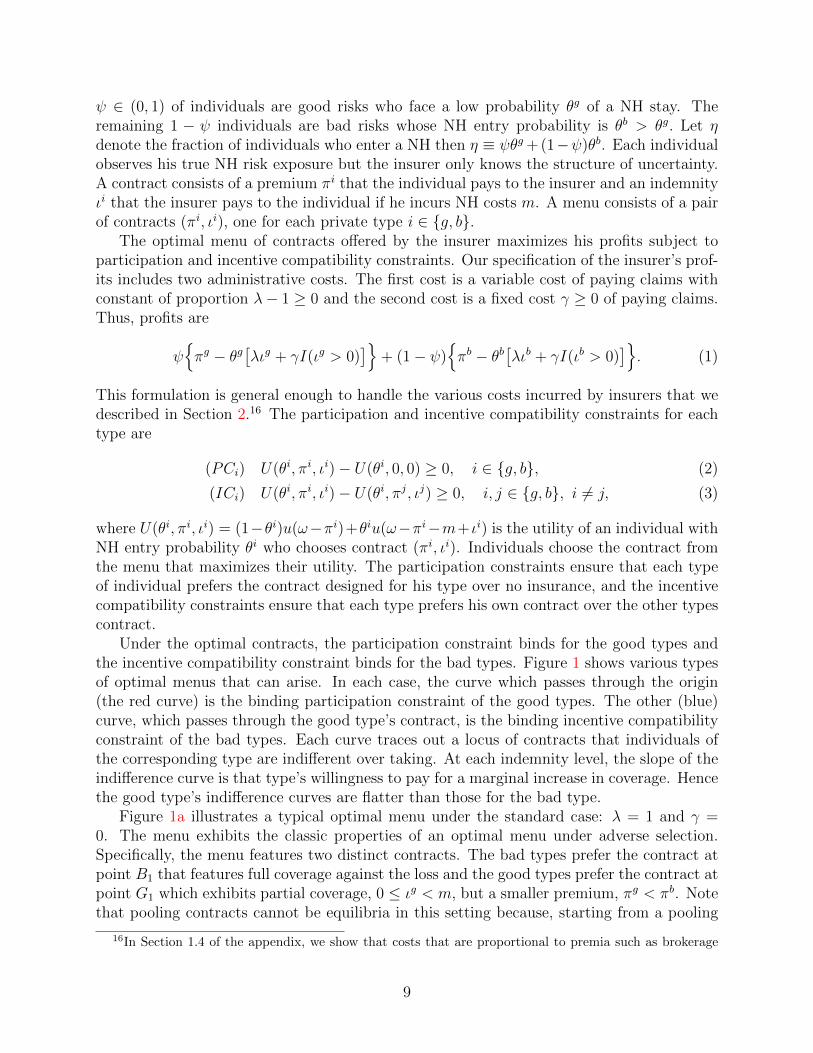
By providing NH residents with a guaranteed consumption floor, Medicaid increases utilityin the absence of private insurance thus reducing demand for such insurance. Moreover,Medicaid is a secondary payer. When cNH > ω−π−m+ ι, marginal increases in the amountof the private LTCI indemnity ι are exactly offset by a reduction in Medicaid transfers, andindividual utility remains constant at u(cNH) = u(cNH). It follows that the marginal utilityof the insurance indemnity is zero for individuals who meet the means-test, and only non-zeroLTCI contracts that satisfy ι− π > cNH +m− ω are potentially attractive to them.

(a) Non-binding consumptionfloor

(b) Low consumption floor (c) High consumption floor

Figure 2: Illustrates the effects of Medicaid on the trading space. The straight lines are theinsurer’s isoprofit lines and the curved lines are the individual’s indifference curves.

Medicaid reduces profits for the insurer but does not impact the extent of coverage offeredto insured individuals within the risk group. In particular, when the risk group is insurable,the bad types always receive full coverage against the NH event. To see this, suppose thatwithout Medicaid, the optimal contract of one of the types is given by point A in Figure 2awith indemnity ι∗. Figure 2b illustrates the impact of introducing Medicaid with a smallvalue of cNH . Notice that the optimal indemnity is unchanged. However, the individual’soutside option has improved, and to satisfy the participation constraint, the premium isreduced. Because the insurer gives the individual the same coverage at a lower price, hisprofits decline.

As cNH increases, an equilibrium, such as the one depicted in Figure 2c, will eventuallyoccur. In this case, cNH is so large that the insurer cannot give the agent an attractiveenough positive contract and still make positive profits. As a result, the individual is deniedcoverage. The same logic obtains when there are two private information types. It followsthat Medicaid can also induce the insurer to deny coverage to the entire risk group. Thisoccurs when the Medicaid consumption floor is large relative to the individual’s endowmentnet of the cost of NH care.

In practice, at the time of LTCI purchase, most individuals do not know how muchwealth they will have at the time a NH event occurs and are, thus, uncertain about whetherand to what extent Medicaid will cover their costs if they experience a NH stay. As we nowillustrate, modeling this uncertainty affects the amount of coverage that individuals demand.

optimal menu to consist of a pooling (0, 0) contract.

12

Suppose that when individuals are choosing their LTCI contract, they face uncertainty aboutthe size of their endowment. Specifically, let ω be distributed with cumulative distributionfunction H(·) over the bounded interval Ω ≡ [ω, ω] ⊂ IR+ with ω ≥ m so that LTCI is alwaysaffordable. Then an individual’s utility function is given by

U(θi, πi, ιi) =

∫ ω

ω

[θiu(ciNH(ω)) + (1− θi)u(cio(ω))

]dH(ω), (6)

where

cio(ω) = ω − πi, (7)

ciNH(ω) = ω + TR(ω, πi, ιi)− πi −m+ ιi, (8)

and the Medicaid transfer is defined by (4).When endowments are random, NH entrants may only be eligible for Medicaid under

smaller realizations of the endowment. A private LTCI product is thus potentially valuablebecause it provides insurance in the states of nature where the endowment is too large tosatisfy the means-test. However, the individual will not want full private LTCI coveragebecause, due to Medicaid, he is already partially insured against NH risk in expectation.20

We have explained that a risk group is always insurable when administrative costs andMedicaid are absent. However, when either is present, it may be optimal for the insurerto deny coverage to the entire group. Whether a risk group is denied coverage dependson the size of administrative costs and the scale of the Medicaid program. It also dependson the distribution of private information within the risk group. In particular, either anincrease in θb or a mean-preserving increase in the dispersion of private information raisesthe possibility that the entire risk group will be denied coverage.21 A larger dispersion inprivate information makes cross-subsidization more difficult and reduces the profitability ofmenus offering positive insurance to both types. At the same time increasing θb makes choicemenus less profitable.

The quantitative model that follows features administrative costs, Medicaid, and asym-metric information. In addition, it features multiple risk groups that vary both in observablecharacteristics of their members and in the distribution of private information within thegroup. The insurer screens individuals in two ways. First, it conducts risk-group selection.In other words, it decides which risk groups to insure and which ones to deny coverage.Second, it chooses the menu of contracts to offer to insurable risk groups. The variation inthe distribution of private information across groups impacts risk-group selection. It alsoimpacts the contracts offered to insurable risk groups.

20See Section 1.2 of the appendix for a detailed discussion of this version of the model, and Propositions3 and 4 which provide a sufficient condition for partial coverage contracts and a set of necessary conditionsfor coverage denials.

21Proposition 6 in the appendix describes conditions under which this can occur when administrativecosts are present. We do not have a formal proof for Medicaid due to the non-convexities it creates. Still, ournumerical results indicate that varying the distribution of private information can also result in the entirerisk group being denied coverage if only Medicaid is present instead.

13

Figure 3: Timeline of events in the baseline model.

3.3 The quantitative model

Our goal is to conduct a quantitative analysis of the LTCI market. In particular, we wantto analyze how asymmetric information, administrative costs, and Medicaid influence LTCItakeup rates, comprehensiveness of coverage, and pricing for groups of individuals who differalong two dimensions that are observable to insurers: frailty and wealth. We now describethe model we use to achieve this objective.

3.3.1 Individual’s problem

In the U.S. most individuals purchase private LTCI around the time of retirement. Theirsaving decisions up to this point in time have been influenced not only by their assessmentof NH entry risk, but also by their assessment of the amount of public and private insurancethey can obtain to help them cope with this risk. The distribution of wealth in turn influencesthe optimal contracting problem of the insurer. Those with high wealth have the outsideoption of self-insuring, and those with low wealth have the outside option of relying onMedicaid if they experience a NH event. We capture the fact that wealth is a choice in aparsimonious way by dividing an individual’s life into three periods. In period 1, he worksand decides how much of his income to save for retirement.22 In period 2, he retires, decideswhether to purchase LTCI, and then experiences realizations of consumption demand andsurvival shocks. Finally, in period 3, he experiences a realization of the NH entry shock.

Figure 3 shows the timing of events in the model.23 At birth, an individual draws hisfrailty status f and lifetime endowment of the consumption good w = [wy, wo] which arejointly distributed with density h(f,w). Frailty status and endowments are noisy indicatorsof NH risk. He also observes his probability of surviving from period 2 to period 3, sf,w, whichvaries with f and w, and the menus of LTCI contracts that will be available in period 2. A

22In Section 1.5 of the appendix we show how our 3 period model could be easily mapped into a modelthat allows for more periods during individuals’ working-age before LTCI purchase occurs.

23See Section 1.6 of the appendix for a table summarizing the model parameters.

14

working-aged individual then decides how to divide his earnings, wy, between consumptioncy and savings a. This decision is influenced by Medicaid and also by the structure of LTCIcontracts. Medicaid benefits are means-tested which creates an incentive to save less so thatthe individual can qualify for Medicaid. LTCI contracts vary with assets, and this mayinduce individuals to save more if risk groups with higher assets face lower premia and/ormore comprehensive coverage.

In period 2, the individual receives a pension wo and observes his true risk of entering aNH conditional on surviving to period 3: θif,w, i ∈ g, b with θgf,w < θbf,w. With probabilityψ the individual realizes a low (good) NH entry probability, i = g, and with probability 1−ψhe realizes a high (bad) NH entry probability, i = b. The individual’s true type i ∈ g, b isprivate information. We assume that NH entry probabilities also depend on f and w. Theindividual then chooses a LTCI contract from the menu offered to him by the private in-surer.24 The insurer observes and conditions the menu of contracts offered to each individualon their frailty status, endowments, and assets. We assume that the insurer observes assetsbecause, as we discussed above, LTC insurers are required by regulators in many states toascertain that the LTCI product sold to an individual is suitable (affordable).25 Each menucontains two incentive-compatible contracts: one for the good types and one for the badtypes. A contract consists of a premium πif,w(a) that the individual pays to the insurer andan indemnity ιif,w(a) that the insurer pays to the individual if the NH event occurs.

After purchasing LTCI, individuals experience a demand shock that induces them toconsume a fraction κ of their young endowment where κ ∈ [κ, κ] ⊆ [0, 1] has density q(κ).The demand shock creates uncertainty about the size of wealth at the time of NH entry andthus is important if the model is to attribute partial coverage to Medicaid as we explainedabove. More generally, it allows the model to capture the following features of NH eventsin a parsimonious way. On average, individuals have 18 years of consumption between theirdate of LTCI purchase and their date of NH entry, during which they are exposed to medicalexpense and spousal death risks, among other risks. In addition, the timing of a NH eventis uncertain, and individuals who experience a NH event at older ages are likely to haveconsumed a larger fraction of their lifetime endowment beforehand.

Period 2 ends with the death event. With probability sf,w individuals survive until period3, and with probability 1 − sf,w they consume their wealth and die.26 We model mortalityrisk because it is correlated with frailty and wealth, and it impacts the likelihood of NHentry.

Finally, in period 3 the NH shock is realized, and those who enter a NH pay cost m

24We assume the insurer does not offer insurance to working-age individuals in period 1 because LTCItakeup rates are low among younger individuals. For example, only 9% of LTCI buyers were less than 50years old in 2015 according to LifePlans, Inc. “Who Buys Long-Term Care Insurance? Twenty-Five Yearsof Study of Buyers and Non-Buyers in 2015–2016” (2017).

25The reference in footnote 7 contains a model worksheet for reporting financial assets that is used todetermine suitability. Lewis et al. (2003) reports that 31 States had adopted some form of suitabilityguidelines by 2002 and Chapter 5 of “ Wall Street Instructors Long-term Care Partnerships online trainingcourse” https://www.wallstreetinstructors.com/ce/continuing_education/ltc8/id32.htm explainshow suitability is assessed in the state of Florida.

26There is evidence that individuals anticipate their death. Poterba et al. (2011) have found that mostretirees die with very little wealth, and Hendricks (2001) finds that most households receive very small orno inheritances. This assumption eliminates any desire for agents to use LTCI to insure survival risk.

15

and receive the private LTCI indemnity. NH entrants may also receive benefits from thepublic means-tested LTCI program (Medicaid). Medicaid is a secondary insurer in that itguarantees a consumption floor of cNH to those who experience a NH shock and have lowwealth and low levels of private insurance.

An individual of type (f,w) solves the following maximization problem, where the de-pendence of choices and contracts on f and w is omitted to conserve notation,

U1(f,w) = maxa≥0,cy ,cNH ,co

u(cy) + βU2(a), (9)

with

U2(a) =[ψu2(a, θ

gf,w, π

g, ιg) + (1− ψ)u2(a, θbf,w, π

b, ιb)], (10)

and

u2(a, θi, πi, ιi) =

∫ κ

κ

u(κwy) + α

[sf,w

(θiu(ci,κNH) + (1− θi)u(ci,κo )

)+ (1− sf,w)u(ci,κo )

]q(κ)dκ, (11)

subject to

cy = wy − a, (12)

ci,κo + κwy = wo + (1 + r)a− πi(a), (13)

ci,κNH + κwy = wo + (1 + r)a+ TR(a, πi(a), ιi(a),m, κ)− πi(a)−m+ ιi(a) (14)

where i ∈ g, b, and α and β are subjective discount factors. The parameter β capturesdiscounting between the time individuals enter the working-age and the time of retirement,and the parameter α captures discounting between the time of retirement and the time ofNH entry. The Medicaid transfer is

TR(a, π, ι,m, κ) = (15)

max

0, cNH −[wo + (1 + r)a− κwy − π −m+ ι

],

and r denotes the real interest rate.In the U.S. retirees with low means also receive welfare through programs such as the

Supplemental Security Income program. We capture these programs in a simple way. Aftersolving the agent’s problem above, which assumes that there is only a consumption floor inthe NH state, we check whether they would prefer, instead, to save nothing and consumethe following consumption floors: cNH in the NH state and co in the non-NH state. If theydo, we allow them to do so and assume that they do not purchase LTCI.27

27Modeling the Supplemental Security Income program in this way helps us to generate the low levels ofsavings of individuals in the bottom wealth quintile without introducing additional nonconvexities into theinsurer’s maximization problem.

16

3.3.2 Insurer’s problem

The insurer observes each individual’s endowments w, frailty status f , and assets a. He doesnot observe an individual’s true NH entry probability, θif,w, but knows the distribution ofNH risk in the population and the individual’s survival risk sf,w. We assume that the insurerdoes not recognize that asset holdings depend on w and f via household optimization. Webelieve that this is realistic because most individuals purchase private LTCI relatively latein life. Note that the demand shock, κ, is realized after LTCI is contracted.

The insurer creates a menu of contracts(πif,w(a), ιif,w(a)

), i ∈ g, b for each group of

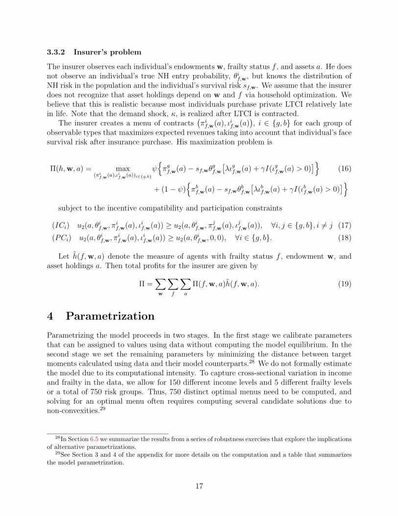
observable types that maximizes expected revenues taking into account that individual’s facesurvival risk after insurance purchase. His maximization problem is

Π(h,w, a) = max(πi

f,w(a),ιif,w(a))i∈g,b

ψπgf,w(a)− sf,wθgf,w

[λιgf,w(a) + γI(ιgf,w(a) > 0)

](16)

+ (1− ψ)πbf,w(a)− sf,wθbf,w

[λιbf,w(a) + γI(ιbf,w(a) > 0)

]subject to the incentive compatibility and participation constraints

(ICi) u2(a, θif,w, π

if,w(a), ιif,w(a)) ≥ u2(a, θ

if,w, π

jf,w(a), ιjf,w(a)), ∀i, j ∈ g, b, i 6= j (17)

(PCi) u2(a, θif,w, π

if,w(a), ιif,w(a)) ≥ u2(a, θ

if,w, 0, 0), ∀i ∈ g, b. (18)

Let h(f,w, a) denote the measure of agents with frailty status f , endowment w, andasset holdings a. Then total profits for the insurer are given by

Π =∑w

∑f

∑a

Π(f,w, a)h(f,w, a). (19)

4 Parametrization

Parametrizing the model proceeds in two stages. In the first stage we calibrate parametersthat can be assigned to values using data without computing the model equilibrium. In thesecond stage we set the remaining parameters by minimizing the distance between targetmoments calculated using data and their model counterparts.28 We do not formally estimatethe model due to its computational intensity. To capture cross-sectional variation in incomeand frailty in the data, we allow for 150 different income levels and 5 different frailty levelsor a total of 750 risk groups. Thus, 750 distinct optimal menus need to be computed, andsolving for an optimal menu often requires computing several candidate solutions due tonon-convexities.29

28In Section 6.5 we summarize the results from a series of robustness exercises that explore the implicationsof alternative parametrizations.

29See Section 3 and 4 of the appendix for more details on the computation and a table that summarizesthe model parametrization.

17

4.1 Highlights of our parametrization strategy

Our main objective is to understand the relative contributions of administrative costs, Med-icaid, and asymmetric information in producing low LTCI takeup rates. We can use directestimates based on data to pin down the scale of administrative costs and Medicaid in ourmodel. However, our direct measure of private information, self-reported NH entry risk, isnoisy. We deal with this issue by parameterizing the model in the following way. First, weassume that administrative costs are identical in all risk groups. Second, we fix the param-eters that govern the scale of administrative costs and Medicaid to reproduce the scale ofthese two factors in the U.S. LTCI market. Third, we fix the overall dispersion in actualNH entry probabilities to reproduce the overall dispersion in self-reported NH entry risk.Finally, we vary the dispersion of private information across risk groups to match the crosssectional pattern of LTCI takeup rates and NH entry rates in our data.

The parameters that govern the scale of Medicaid and administrative costs use datatargets from multiple sources. The scale of Medicaid is determined by the consumption floorprovided to recipients and also the distribution of wealth at the point of NH entry becauseMedicaid benefits are means tested. We set the Medicaid NH consumption floor to the valueused by Brown and Finkelstein (2008) which is based on the dollar value of transfers toMedicaid NH residents. Recall that the κ shock determines the distribution of wealth at thepoint of NH entry. We choose the mean of the κ shock distribution to reproduce the ratioof average wealth at NH entry to average wealth at the time of private insurance purchase,and the variance to reproduce the same ratio for quintile 5. We use the ratio of quintile 5’swealth to pin-down the variance because the extent to which higher wealth individuals haveaccess to Medicaid is key to the relative importance of Medicaid versus the two supply-sidefrictions in accounting for the extent of private insurance. Individuals with low wealth atthe time of insurance purchase are already very likely to get Medicaid benefits in the eventof NH entry regardless of the size of their κ shock.

We set the administrative costs using industry-level data provided by the Society ofActuaries. The fixed cost γ and variable cost parameter λ are chosen so that the modelreproduces industry-level average fixed and variable costs faced by insurers.

Having fixed the scale of Medicaid and administrative costs, the next step is to parametrizethe distribution of private information. We set the fraction of good types, ψ, such that theoverall dispersion in private information in the model is consistent with estimates basedon the data. The only direct measure of private information in HRS data is respondents’self-reported probabilities of entering a NH within the next 5 years. We set ψ such thatthe coefficient of variation of NH entry probabilities in the model matches the coefficient ofvariation of self-reported NH entry probabilities in the HRS data.30

The NH entry probabilities conditional on survival within each risk group, θbf,w, θgf,w,

are pinned-down using data on NH entry by frailty and permanent earnings (PE) and data

30Ideally, we would like to use data on dispersion in self-reported NH entry risk by frailty and wealthto pin down the variation in dispersion across risk groups. However, this measure of private information isnoisy, especially as sample sizes decline, and does not measure individuals’ lifetime NH entry risk. For thesereasons, we do not use it to parametrize θbf,w, θ

gf,w. Instead, in Section 5, we use this data to assess our

parametrization.

18

1 2 3 4 5Frailty quintile

0

0.05

0.1

0.15

0.2

0.25

0.3

LTC

I tak

e-up

rat

ewealth quintile 1wealth quintile 2wealth quintile 3wealth quintile 4wealth quintile 5

1 2 3 4 5Frailty quintile

0.25

0.3

0.35

0.4

NH

ent

ry p

roba

bilit

y

PE quintile 1PE quintile 2PE quintile 3PE quintile 4PE quintile 5

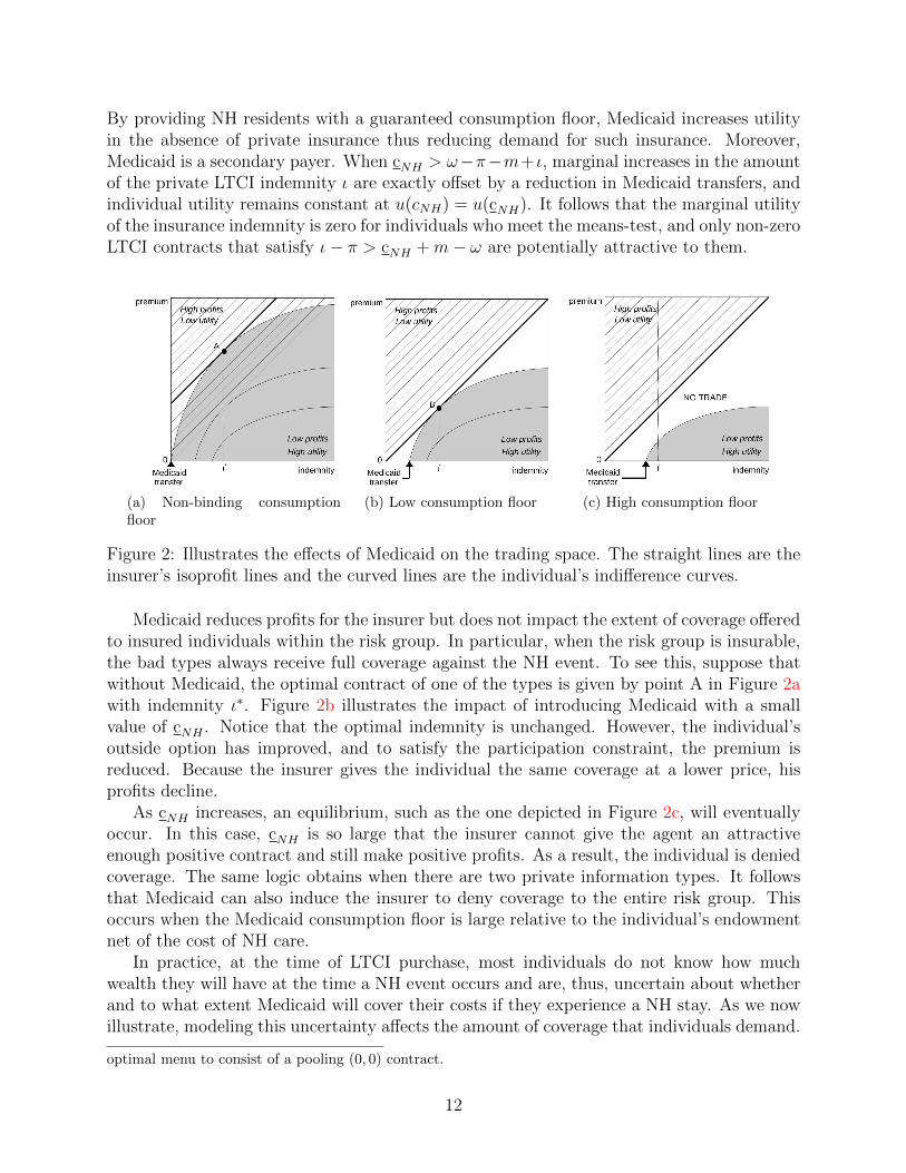
Figure 4: LTCI takeup rates by wealth and frailty quintiles (left panel) and the probabilitythat a 65-year old will ever enter a NH by frailty and PE quintiles (right panel). LTCItakeup rates are for 62–72 year-olds in our HRS sample. NH entry probabilities are for a NHstay of at least 100 days and are based on our auxiliary simulation model which is estimatedusing HRS data. Frailty, wealth, and PE all increase from quintile 1 to quintile 5. Thewealth quintiles reported here are marginal and not conditional on the frailty quintile, so forexample only around 7% of people in frailty quintile 1 are in wealth quintile 1, while 33%are in wealth quintile 5.

on LTCI takeup rates by frailty and wealth.31 The left panel of Figure 4 shows the LTCItakeup rates of HRS respondents by frailty and wealth quintiles. LTCI takeup rates arelow, 9.4% on average, decline with frailty and increase with wealth.32 The right panel ofFigure 4 shows how the lifetime NH entry probability of a 65 year-old varies across frailtyand PE quintiles.33 Notice that NH entry risk does not vary much with frailty within eachPE quintile. It is essentially flat in PE quintiles 4 and 5, and decreases slightly in quintiles1–3. Also notice that NH entry does not vary much by PE within frailty quintiles. It isslightly decreasing in PE in frailty quintiles 1–3, and there is essentially no variation infrailty quintiles 4 and 5. These patterns occur because frailty and PE are good indicators ofboth NH entry risk and mortality risk.

To illustrate how the model adjusts θbf,w, θgf,w to simultaneously account for the patterns

of NH entry and LTCI takeup, consider PE/wealth quintiles 4 and 5. LTCI takeup ratesdecline with frailty in these two quintiles but the mean probability of NH entry does notvary. The only way to generate both of these patterns in the model is if the dispersionin private information, and thus the severity of the adverse selection problem, increases

31We use annuitized income to proxy for PE and assign individuals the annuitized income of their house-hold head. See Section 2 of the appendix for details.

32The pattern of LTCI takeup rates by frailty and wealth is robust to controlling for marital status andwhether or not individuals have any children. See Section 2.4 of the appendix for details.

33 Lifetime NH entry probabilities by frailty and PE quintile groups were obtained using an auxiliarysimulation model similar to that in Hurd et al. (2013) and our HRS data. All NH entry probabilities areprobabilities of experiencing a long-term (at least 100 day) NH stay. We focus on long-term NH stays becausestays of less than 100 days are heavily subsidized by Medicare.

19

with frailty within these two PE/wealth quintiles. In other words, the dispersion in NHentry probabilities conditional on surviving, θgf,w, θbf,w, must go up. To provide a secondexample, observe that, in frailty quintiles 4 and 5, LTCI takeup rates increase with wealthbut mean NH entry probabilities do not vary with PE. To account simultaneously for thesetwo observations, the dispersion in θgf,w, θbf,w must decline with PE/wealth in these frailtyquintiles.

Our strategy for parametrizing ψ and θgf,w, θbf,w allows us to determine the extent towhich low LTCI takeup rates are due to choice menus offered to insurable risk groups versusrisk-group selection. To see this, consider two alternative schemes for matching the patternof takeup rates in the data. The first scheme is to have a large differential in NH entrybetween good and bad types (large θb to θg ratios within each risk group), but few bad types(a high ψ). The second scheme is to have many bad types (a low ψ), but a smaller differentialin NH entry between good and bad types (small θb to θg ratios within each risk group). Inour model, coverage denials play a relatively larger role in generating low takeup rates underthe first scheme, while choice menus play a relatively larger role under the second. Riskgroup denials play a larger role under the first scheme because the large differential betweenθb and θg makes cross-subsidizing menus unprofitable but large θb also makes choice menusunprofitable. Choice menus in insurable risk groups play a larger role under the secondscheme because the large fraction of bad types makes cross-subsidizing menus unprofitable,but lower θb means the insurer can still make profits by insuring bad types on their own.Thus, choice menus are still profitable.

Consistently, in Section 6.5, we document that lowering ψ and then reparametrizingθgf,w, θbf,w to match the LTCI takeup rates results in a higher fraction of individuals beingoffered choice menus. However, this second scheme also produces too little overall dispersionin private information. In practice, the reduction in dispersion due to reducing the ratios ofθb to θg within risk groups dominates the increase in dispersion due to reducing ψ. Thus, byreproducing the overall dispersion in private information in the data we are able to identifythe relative role of risk-group selection versus choice menus in generating low LTCI takeuprates.

4.2 Functional forms and first stage calibration

We assume constant-relative-risk-aversion utility such that

u(c) =c1−σ

1− σ.

Individuals cover a substantial fraction of NH expenses using their own resources. Given thesize of these expenses, it makes sense to assume that households are risk averse and thuswilling to pay a premium to avoid this risk. A common choice of the risk aversion coefficientin the macroeconomics incomplete markets literature is σ = 2. We use this value.

The distribution of frailty in the model is calibrated to replicate the distribution of frailtyof individuals aged 62–72 in our HRS sample. We focus on 62–72 year-old individuals becausefrailty is observed by the insurer at the time of LTCI purchase. In our HRS sample, thefrailty of 62–72 year-old individuals is negatively correlated with their PE. To capture thisfeature of the data we assume that the joint distribution of frailty and the endowment stream,

20

Table 1: Mean frailty by PE quintile in the data and the model.

PE Quintile1 2 3 4 5

Data 0.23 0.22 0.19 0.17 0.15Model 0.23 0.20 0.19 0.17 0.15

Data source: Authors’ calculations using our HRS sample.

0 0.1 0.2 0.3 0.4 0.5 0.6 0.7 0.8 0.9Frailty

0

0.05

0.1

0.15

0.2

0.25

Figure 5: Distribution of frailty for 62–72 year-olds in our HRS sample. Severity of frailtyis increasing with the index value and the maximum is normalized to one.

h(f,w), is a Gaussian copula. This distribution has two attractive features: the marginaldistributions do not need to be Gaussian and the dependence between the two marginaldistributions can be summarized by a single parameter ρf,w. The value of this parameter isset to −0.29 so that the variation in mean frailty by PE quintile in the model is as observedin the data. Table 1 shows the data values and model counterparts.

Figure 5 shows the empirical frailty distribution. We approximate it using a beta distri-bution with a = 1.54 and b = 6.30. The parameters of the distribution are chosen such thatmean frailty in the model is 0.19 and the Gini coefficient of the frailty distribution is 0.34,consistent with their counterparts in the data. When computing the model, we discretizefrailty into a 5-point grid. We use the mean frailty of each quintile of the distribution asgrid values.

The marginal distribution of endowments is assumed to be log-normal. We equate en-dowments to the young with permanent earnings and normalize the mean young endowmentto 1. This is equivalent to a mean permanent earnings of $1,049,461 in year 2000 whichis approximated as average earnings per adult aged 18–64 in year 2000 multiplied by 40years.34 The standard deviation of the log of endowments to the young is set to 0.8 becauseit implies that the Gini coefficient for the young endowment distribution is 0.43. This value

34To derive average earnings per adult aged 18-64 in year 2000 we divide aggregate wages in 2000 takenfrom the Social Security Administration by number of adults aged 18-64 in 2000 taken from the U.S. Census.

21

is consistent with the Gini coefficient of the permanent earnings distribution for individuals65 and older in our HRS sample.

Endowments to the old are a stand in for retirement income which is comprised primar-ily of income from social security and private pension benefits. We assume that the incomereplacement ratio (retirement income relative to pre-retirement income) is linear in logs.Purcell (2012) calculates income replacement ratios for HRS respondents. Using his calcu-lations, we set the level and slope of the replacement rate function such that the medianreplacement rate of retirees in the bottom pre-retirement income quartile is 64% and themedian rate for retirees in the top quartile is 50%.35 The resulting average replacement ratein the baseline economy is 57%.

The consumption demand shock, κ, captures the uncertainty individuals face at the timeof LTCI purchase about their resources later in life when a NH event may occur. Thisuncertainty is, in part, due to uncertainty about the date of NH entry itself. Since thedistribution of NH entry ages is left-skewed, we assume that the distribution of the κ shock,q(κ), is also left-skewed.36 This is achieved by setting q(κ) such that 1−κ has a truncated log-normal distribution over [0.2, 0.8].37 The mean and variance of κ, µκ and σ2

κ, are determinedin the second stage.

We estimate the risk of a long-term stay in a NH using HRS data and the questions inthat survey do not distinguish between stays in skilled nursing facilities (SNF) and staysin assisted living communities or residential care centers (RCC). Thus, when estimatingthe average cost of a NH stay we take a weighted average of SNF and RCC expenses. Inpractice residential LTC expenses have two components. The first component is nursing andmedical care and the second component is room and board. We interpret the room and boardcomponent as being part of consumption and thus a choice and not an expense shock. Usingdata from a variety of sources, we estimate that the average medical and nursing expensecomponent of residential LTC costs was $32,844 per annum in 2000 and the average benefitperiod was 2.976 years. Multiplying the annual medical and nursing cost by the averagebenefit period yields total medical expenses of $97,743 or a value of m of 0.0931 when scaledby mean permanent earnings.38

We set the consumption floor provided by Medicaid, cNH , and the consumption floor forthose who do not enter a NH, co, to the same value: $6,540 a year. As mentioned above, thisvalue is taken from Brown and Finkelstein (2008) and consists of a consumption allowanceof $30 per month and housing and food expenses of $515 per month. The former number isbased on Medicaid administrative rules and the latter figure was the monthly amount thatSSI paid a single elderly individual in 2000. We assume that the third period of the modelhas the same length as the average duration of long-term NH stays. Thus, we multiply theannual consumption floor by 2.976 years to come up with the total size of the consumptionfloor. The resulting value of cnh is 1.855% of mean permanent earnings.

Having calibrated the joint distribution of frailty and the endowment stream, h(f,w), weuse it to assign individuals in the model to frailty and PE quintiles, and thereby partition

35These estimates are the median replacement rates of retirees who have been retired for at least 6 years.See Purcell (2012), Table 4.

36Murtaugh et al. (1997) estimate the distribution of NH entry ages.37The baseline parametrization is robust to expanding the range of κ values within [0, 1].38See Section 4 of the appendix for details and data sources.

22

the population into 25 groups, one for each frailty/PE quintile combination. To reduce thenumber of parameters, we assume that individuals within the same group have the samesurvival probability sf,w and the same set of NH entry probabilities θbf,w, θ

gf,w.39

The 25 survival probabilities are set to the probability that a 65 year-old will surviveto either age 80 or until a NH event occurs.40 We use survival until age 80 or a NH eventbecause this way, regardless of which one we target, our parametrized model will match boththe unconditional NH entry probabilities reported in Figure 4 and NH entry probabilitiesconditional on survival which we report in Section 4 of the appendix. The resulting sur-vival probabilities of each frailty and PE quintile are also reported in the appendix. Notsurprisingly, the relationship between frailty and survival is negative in all PE quintiles.

Finally, the risk-free real return, r, is not separately identified from the preference dis-count factor β. We normalize it to 0% per annum.41

4.3 Second stage: simulated moment matching strategy

The set of parameters left to pin down are the preference discount factors (β, α), the con-sumption shock distribution parameters (µκ, σκ), the administrative cost parameters (λ, γ),the fraction of good types ψ, and the 25 NH entry probability pairs: θbf,w, θ

gf,w for each

frailty/PE quintile combination. These parameters are chosen to minimize the distancebetween equilibrium moments of the model and their data counterparts. Even though allof these parameters are chosen simultaneously through the minimization procedure, eachparameter has a specific targeted moment.

The preference discount factor, β, in conjunction with the interest rate and σ determineshow much people save for retirement. It is chosen such that the model reproduces the averagewealth of 62–72 year olds in our HRS sample relative to average lifetime earnings. This valueis 0.222 in the data and 0.229 in the model. The resulting annualized value of β is 0.94.42

On average individuals in our dataset enter a NH at age 83 or about 18 years after theyretire. The parameter α captures the discounting between the age of retirement and LTCIpurchase, and the age when a NH event is likely to occur. The more that individuals discountthe NH entry period, the larger the fraction of NH residents who will be on Medicaid. Thusour choice of α targets the Medicaid recipiency rate of NH residents in our HRS sample.The target rate is 46%, the model rate is 48%, and the value of α is 0.20.43 Eighteen yearsbetween age 65 and NH entry implies that the annualized value of α is 0.91.

We set the consumption shock distribution parameters, (µκ, σκ), to target two data facts.The first data target is the average wealth of NH entrants immediately before entering the

39We wish to emphasize that these groups are not risk groups because individuals in a given group arenot identical to the insurer. The insurer observes 150 distinct levels of permanent earnings and thus willoffer different menus to individuals in a given group.

40Survival probabilities by frailty and PE quintiles are estimated using HRS data and our auxiliarysimulation model. See footnote 33.

41This normalization only impacts the value of β and for our analysis, which does not involve any welfarecalculations, is innocuous.

42Our choice of this age group is based on two considerations. First, if we limit attention to those aged65 we would only have a small number of observations. Second, the average age when individuals purchaseLTCI in our sample is 67 and this is the midpoint of the interval we have chosen.

43Our Medicaid recipiency rate target is lower than other estimates. But, this reflects the fact that in

23

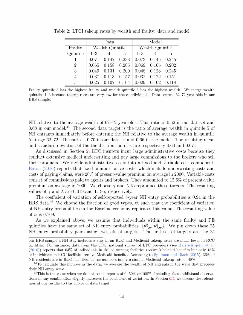
Table 2: LTCI takeup rates by wealth and frailty: data and model

Data ModelFrailty Wealth Quintile Wealth Quintile

Quintile 1–3 4 5 1–3 4 51 0.071 0.147 0.233 0.073 0.145 0.2452 0.065 0.158 0.205 0.069 0.165 0.2023 0.049 0.131 0.200 0.048 0.128 0.2454 0.037 0.113 0.157 0.032 0.122 0.1515 0.025 0.107 0.104 0.029 0.102 0.118

Frailty quintile 5 has the highest frailty and wealth quintile 5 has the highest wealth. We merge wealthquintiles 1–3 because takeup rates are very low for these individuals. Data source: 62–72 year olds in ourHRS sample.

NH relative to the average wealth of 62–72 year olds. This ratio is 0.62 in our dataset and0.68 in our model.44 The second data target is the ratio of average wealth in quintile 5 ofNH entrants immediately before entering the NH relative to the average wealth in quintile5 at age 62–72. The ratio is 0.70 in our dataset and 0.66 in the model. The resulting meanand standard deviation of the the distribution of κ are respectively 0.60 and 0.071.

As discussed in Section 2, LTC insurers incur large administrative costs because theyconduct extensive medical underwriting and pay large commissions to the brokers who selltheir products. We divide administrative costs into a fixed and variable cost component.Eaton (2016) reports that fixed administrative costs, which include underwriting costs andcosts of paying claims, were 20% of present-value premium on average in 2000. Variable costsconsist of commissions paid to agents and brokers. They amounted to 12.6% of present-valuepremium on average in 2000. We choose γ and λ to reproduce these targets. The resultingvalues of γ and λ are 0.019 and 1.195, respectively.

The coefficient of variation of self-reported 5-year NH entry probabilities is 0.94 in theHRS data.45 We choose the fraction of good types, ψ, such that the coefficient of variationof NH entry probabilities in the Baseline economy replicates this value. The resulting valueof ψ is 0.709.

As we explained above, we assume that individuals within the same frailty and PEquintiles have the same set of NH entry probabilities, θbf,w, θ

gf,w. We pin down these 25

NH entry probability pairs using two sets of targets. The first set of targets are the 25

our HRS sample a NH stay includes a stay in an RCC and Medicaid takeup rates are much lower in RCCfacilities. For instance, data from the CDC national survey of LTC providers (see Harris-Kojetin et al.(2016)) reports that 63% of individuals in skilled nursing facilities receive Medicaid benefits but only 15%of individuals in RCC facilities receive Medicaid benefits. According to Spillman and Black (2015), 36% ofNH residents are in RCC facilities. These numbers imply a similar Medicaid takeup rate of 48%.

44To calculate this number in the data, we average the wealth of NH entrants in the wave that precedestheir NH entry wave.

45This is the value when we do not count reports of 0, 50% or 100%. Including these additional observa-tions in any combination slightly increases the coefficient of variation. In Section 6.5, we discuss the robust-ness of our results to this choice of data target.

24

1 2 3 4 5Frailty quintile

0

0.2

0.4

0.6

0.8

1

NH

ent

ry p

roba

bilit

y

bad types

good types

PE quintile 1PE quintile 2PE quintile 3PE quintile 4PE quintile 5

Figure 6: Nursing home entry probabilities conditional on surviving for good and bad typesby frailty and PE quintile in the Baseline economy.

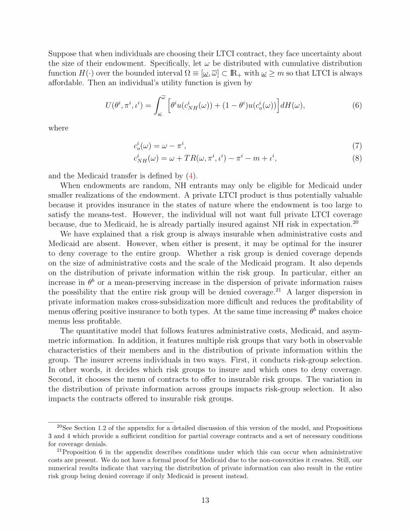
probabilities of entering a NH for a lifetime stay by frailty/PE quintile combination reportedin the right panel of Figure 4. By targeting these probabilities we are ensuring that theaverage NH entry probability in each frailty/PE quintile group replicates its estimated valuebased on the HRS data. The second set of targets are the 15 LTCI takeup rates of individualsin all combinations of quintiles 1–3, 4, and 5 of the wealth distribution and quintiles 1 through5 of the frailty distribution reported in the lower panel of Table 2. In order to identify these50 parameters using only 40 moments, we assume that the ratio of NH entry probabilitieswithin a risk group is constant across wealth quintiles 1–3 within each frailty quintile.46 Ourdecision to restrict the parameters in this way is based on two considerations. First, recallfrom Figure 4 that only a very small number of individuals in quintiles 1 and 2 have LTCIin our dataset. Second, in the model, no individuals in these quintiles buy LTCI becausethey are guaranteed to get Medicaid if they incur a NH event.47 The resulting NH entryprobability pairs are displayed in Figure 6. Observe that the dispersion in the θ′s increaseswith frailty but declines with PE. From this we see that the model is indeed assigning abigger role to private information in frail and poor risk groups as we suggested in Section4.1.

Table 2 reports the 15 LTCI takeup rates in the Baseline economy. The fit of the modelis not perfect due to the fact that we discretize the state space to compute the model. Note,however, that the takeup rates generated by the model increase with wealth and declinewith frailty for both the rich and poor. The model also does a good job of reproducing theaverage LTCI takeup rate. In our HRS sample, 9.4% of retirees aged 62–72 have LTCI andin the model 9.7% of 65 year-olds have a nonzero LTCI contract. The fact that we are able

46Specifically, we assume that θbf,w/θgf,w is constant across wealth quintiles 1–3 within each frailty quintile.This produces 10 restrictions such that, together with the 40 other moments, the 50 parameters are exactlyidentified.

47This difference between the model and the data is present for a variety of reasons including measurementerror, our parsimonious specification of the Medicaid transfer function, and the fact that we have not modeledall shocks faced by retirees such as spousal death.

25

Table 3: Standard deviation of self-reported (private) NH entry probabilities by frailty andpermanent-earnings quintiles: data and model

Frailty Quintile1 2 3 4 5

Data 1.00 1.00 1.03 1.27 1.47Model 1.00 1.08 1.20 1.31 1.47

Permanent Earnings Quintile1 2 3 4 5

Data 1.00 0.92 0.85 0.79 0.76Model 1.00 0.96 0.91 0.78 0.59

The standard deviations (SDs) are normalized such that the SD of frailty quintile 1 is 1. Data values areSDs of self-reported probabilities of entering a NH in the next 5 years for individuals aged 65–72 excludingobservations where the probability is 0, 100% or 50%. The pattern in the data is robust to variations in theway we construct the SDs including how we handle those reporting a probability of 0, 100% or 50%. Datasource: Authors’ calculations using our HRS sample.

to reproduce the average LTCI takeup rate suggests that the restrictions we have imposedon the θbf,w’s for wealth quintiles 1-3 are broadly consistent with our data.

5 Assessing the model parametrization

Dispersion of private information by frailty and permanent earnings. One way toassess this aspect of our model is to provide independent evidence that dispersion in privateNH entry probabilities, and thus the severity of the private information friction, increaseswith frailty and decreases with PE. The first and third rows of Table 3 report normalizedstandard deviations of self-reported NH entry probabilities for 65–72 year-old HRS respon-dents by frailty and PE quintile. These probabilities are not exactly comparable to theprivate NH entry probabilities in the model for two reasons. First, they are self-reportedprobabilities of NH entry in the next 5 years whereas the model values are lifetime NH entryprobabilities. Second, the self-reported probabilities are noisy and in some instances sensitiveto how one cleans the data. For instance, 1/3 of respondents report 0.5 and another thirdreport either 0 or 1 in the raw data. We choose to omit these responses. The second andfourth rows of the table report the distribution of private NH entry probabilities by frailtyand PE quintile that emerge from the model. Despite the noise, the dispersion of privateinformation is increasing in frailty and decreasing in PE in both the data and the model.This pattern of dispersion is consistent with Hendren (2013)’s findings, discussed in Section2.2, that adverse selection is more severe among individuals that are more likely to deniedcoverage by LTC insurers. Notice finally that the magnitudes of the normalized standarddeviations in the model are reasonably close to their corresponding values in the data.

26

Table 4: Distribution of insurance across NH residents: data and model

LTCI Medicaid Both Neither

Data 8.1 45.6 1.4 44.2Model 9.5 47.6 0.3 42.6

Percent of NH residents covered by LTCI only, Medicaid only, both, or neither in the data and the model.Data source: Authors’ calculations using our HRS sample.

Distribution of insurance. Table 4 shows the distribution of insurance across NH resi-dents in the model and the HRS data. None of these moments were explicitly targeted whenparametrizing the model. Yet, the fit between the model and data is very good. The modeleven predicts that some NH residents receive both private LTCI and Medicaid benefits. Inthe model, these are individuals who, ex-ante, bought LTCI because they would not be cov-ered by Medicaid for all realizations of the demand shock but, ex-post, drew a realization ofκ that resulted in Medicaid eligibility.

Pricing and coverage of LTCI. Pricing and coverage statistics were not targeted whenparametrizing the model. It is thus noteworthy that the average pricing and coverage levelsof LTCI in our model are consistent with observations from the U.S. LTCI market. Recallthat Brown and Finkelstein (2007) and Brown and Finkelstein (2011) find that the averageload in the LTCI market is in the range 0.18 and 0.5, depending on whether or not theloads are adjusted for policy lapses in the sample period. The average load in our model at0.41 falls in middle of this range. In Section 2 we explained that typical coverage levels forLTCI products range between one-third and two-thirds of expected lifetime NH expenses.Insurance contracts in our model offer indemnities that cover on average 58% of NH medicalcosts.

Brown and Finkelstein (2007) also find that the relationship between loads and compre-hensiveness is non-monotonic and that for some individuals loads are negative. Table 5,shows that average loads and coverage do not vary systematically with wealth. However,average loads are increasing in frailty and coverage levels are declining in frailty. Thus, frailindividuals pay more for LTCI and receive less coverage according to the model.

Table 5 also reports coverage and loads by private information type. It is immediatelyclear from these results that, as in Stiglitz (1977), the insurer offers bad-risk types in insurablerisk groups more coverage at a lower unit price. In virtually all wealth and frailty quintiles,bad types have negative loads indicating that they are getting a good deal relative to theactuarially fair benchmark. Good types, in contrast, have large and positive loads at allwealth and frailty quintiles. The combination of negative loads for bad types and positiveloads for good types highlights the fact that the optimal contracts feature cross-subsidization.Revenues from good types are used by the insurer to subsidize contracts to bad types withina given risk group.

In the model, the insurer is free to create a separate menu for each risk group and, inequilibrium, offers hundreds of risk-group-specific menus. Table 5 indicates that, on the one

27

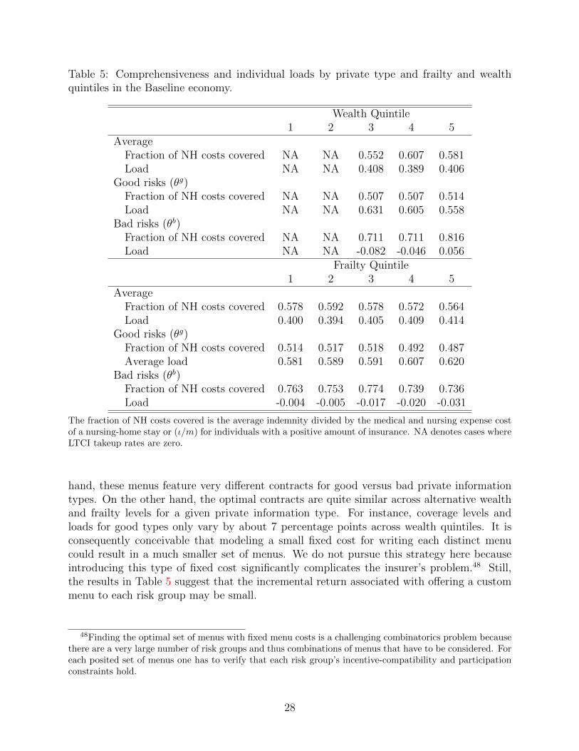
Table 5: Comprehensiveness and individual loads by private type and frailty and wealthquintiles in the Baseline economy.

Wealth Quintile1 2 3 4 5

AverageFraction of NH costs covered NA NA 0.552 0.607 0.581Load NA NA 0.408 0.389 0.406

Good risks (θg)Fraction of NH costs covered NA NA 0.507 0.507 0.514Load NA NA 0.631 0.605 0.558

Bad risks (θb)Fraction of NH costs covered NA NA 0.711 0.711 0.816Load NA NA -0.082 -0.046 0.056

Frailty Quintile1 2 3 4 5

AverageFraction of NH costs covered 0.578 0.592 0.578 0.572 0.564Load 0.400 0.394 0.405 0.409 0.414

Good risks (θg)Fraction of NH costs covered 0.514 0.517 0.518 0.492 0.487Average load 0.581 0.589 0.591 0.607 0.620

Bad risks (θb)Fraction of NH costs covered 0.763 0.753 0.774 0.739 0.736Load -0.004 -0.005 -0.017 -0.020 -0.031

The fraction of NH costs covered is the average indemnity divided by the medical and nursing expense costof a nursing-home stay or (ι/m) for individuals with a positive amount of insurance. NA denotes cases whereLTCI takeup rates are zero.

hand, these menus feature very different contracts for good versus bad private informationtypes. On the other hand, the optimal contracts are quite similar across alternative wealthand frailty levels for a given private information type. For instance, coverage levels andloads for good types only vary by about 7 percentage points across wealth quintiles. It isconsequently conceivable that modeling a small fixed cost for writing each distinct menucould result in a much smaller set of menus. We do not pursue this strategy here becauseintroducing this type of fixed cost significantly complicates the insurer’s problem.48 Still,the results in Table 5 suggest that the incremental return associated with offering a custommenu to each risk group may be small.

48Finding the optimal set of menus with fixed menu costs is a challenging combinatorics problem becausethere are a very large number of risk groups and thus combinations of menus that have to be considered. Foreach posited set of menus one has to verify that each risk group’s incentive-compatibility and participationconstraints hold.

28

6 Results

6.1 LTCI takeup rates and denials

There are two different ways that low LTCI takeup can arise in the model. One way is throughchoice menus. Recall that a choice menu consists of two contracts: a non-zero contract anda (0, 0) contract. As we explained above, under these types of menus, good-risk types choosethe no-insurance (0, 0) contract. The other way is via risk-group selection. Recall thatrisk-group selection will occur when all individuals in some risk groups are uninsurable and,hence, denied coverage by the insurer. It turns out that only 0.11% of individuals choose notto purchase LTCI. Thus, in the model, low LTCI takeup rates are primarily due to risk-groupselection. Consistently, as the first column of Table 6 shows, the denial rate in our Baselineeconomy is 90.1%. It is 100% for individuals in PE quintiles 1 and 2 and declines withpermanent earnings in quintiles 3–5. However, the denial rates are non-monotonic amongthe highest PE individuals. Denial rates are only 58.8% among individuals in the top 5% ofPE but then rise to 100% for those in the top 1%. Individuals with the highest PE preferto self-insure NH risk.

The pattern of denials reported in the first column of Table 6 is consistent with the esti-mates of denial rates that we reported in Section 2. Denial rates decline with wealth in boththe model and the data. Denial rates in the model are much larger than our estimated denialrates reported in Section 2 which range from 36% to 56% for 55–66 year old HRS respon-dents. Our estimated denial rates only capture denials that arise as a result of informationrevealed during medical underwriting. However, there are other reasons why a risk groupmay be uninsurable. For instance, all individuals in healthy, but poor, risk-groups may beuninsurable because they know they will qualify for Medicaid. Similarly, all individuals inhealthy, high- income risk-groups may be uninsurable because they prefer to self-insure sinceLTCI is costly to produce. Survey results in Ameriks et al. (2016) suggest that the highcost of LTCI is also an important reason for low takeup rates. In general, a risk group isuninsurable if no profitable positive insurance contract exists that at least one individual inthe risk group is willing to take.

6.2 Insurance ownership and NH entry

Our finding on the quantitative significance of denials raises the possibility that empiricaltests for adverse selection based on estimated correlations between insurance ownership andloss occurrence may have weak power. These tests are based on the standard theory ofadverse selection with a single source of private information which predicts that, if adverseselection is present in the market, LTCI owners should have higher NH entry rates than non-owners (see Chiappori and Salanie (2000)). As we discussed in Section 2.2, Finkelstein andMcGarry (2006) use these empirical tests to test for adverse selection in the U.S. LTCI mar-ket. They find that LTCI owners, if anything, have lower NH entry rates than non-owners.Their result is striking because they also find that individuals have private information abouttheir NH risk and that they act on this risk by purchasing LTCI.

Finkelstein and McGarry (2006) conclude that, to reconcile their conflicting set of find-ings, there must be multiple sources of private information present in the U.S. LTCI market.

29

Table 6: Denial rates in the Baseline, the No Administrative Costs, the No Medicaid, andthe Full Information Economies

Scenario Baseline No Admin. Costs No Medicaid Full InformationDescription λ = 1, γ = 0 cnh = 0.001 θif,w public

Average 90.1 38.7 9.4 62.5By PE Quintile

1 100 100 27.4 1002 100 93.4 0.0 99.63 85.7 0.0 0.0 54.14 83.9 0.0 0.0 29.15 81.2 0.0 19.8 29.7

High PEtop 10 75.1 0.0 39.5 30.4top 5 58.8 0.0 76.2 31.7top 1 100 0.0 100 100

By receiving Medicaid NH benefits conditional on survivingWould 47.6 37.0 5.5 43.9Would not 42.5 1.6 4.0 18.6

Denial rates are percentage of individuals who are only offered a single contract of (0, 0) by the insurer. Notethat, in the first nine rows, the figures are the percentage of individuals in that group. However, the bottomtwo rows of the table are a decomposition of the average denial rate for that economy.

Interestingly, our model with a single source of private information and an active extensivecontracting margin generates each of their empirical results. First, Finkelstein and McGarry(2006) find a positive correlation between self-assessed NH entry risk and NH entry, evenafter controlling for observable health, and interpret this as evidence of private information.We have explicitly modeled private information and adverse selection and, as Figure 6 shows,our model delivers this correlation by construction. Second, they find that individuals acton their private information by documenting a positive correlation between self-assessed NHentry risk and LTCI ownership. The baseline economy has this property too. The LTCI own-ership rate of bad types is 10.6% while the ownership rate of good types is 10.2%. Moreover,bad types have a higher LTCI ownership rate than good types no matter whether or howwe control for the information set of the insurer, or whether or not we condition on survival.Third, the correlations between LTCI ownership and NH entry rates in the Baseline economyare small and can be negative. Table 7 reports NH entry rates conditional on survival ofLTCI owners and non-owners. Only 36.9% of LTCI owners in the Baseline economy enter a

49We believe that the NH entry rates conditional on survival are the most comparable to Finkelstein andMcGarry (2006)’s findings given that they only look at NH entry within 5 years of observed LTCI ownership.That said, with no controls, our model still generates a negative, albeit smaller, correlation even if we donot condition on survival. The reason conditioning on survival matters is because it impacts the correlationbetween average NH entry and LTCI takeup rates across risk groups (see Figure 4).

30

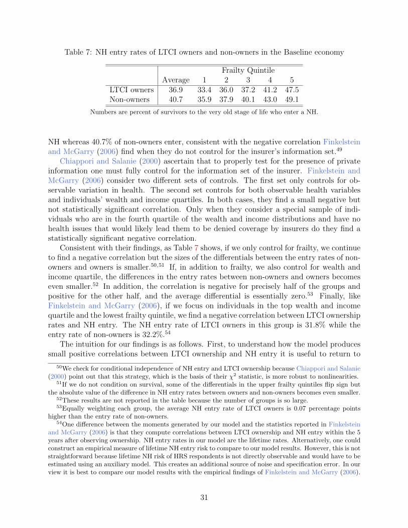
Table 7: NH entry rates of LTCI owners and non-owners in the Baseline economy

Frailty QuintileAverage 1 2 3 4 5

LTCI owners 36.9 33.4 36.0 37.2 41.2 47.5Non-owners 40.7 35.9 37.9 40.1 43.0 49.1

Numbers are percent of survivors to the very old stage of life who enter a NH.

NH whereas 40.7% of non-owners enter, consistent with the negative correlation Finkelsteinand McGarry (2006) find when they do not control for the insurer’s information set.49

Chiappori and Salanie (2000) ascertain that to properly test for the presence of privateinformation one must fully control for the information set of the insurer. Finkelstein andMcGarry (2006) consider two different sets of controls. The first set only controls for ob-servable variation in health. The second set controls for both observable health variablesand individuals’ wealth and income quartiles. In both cases, they find a small negative butnot statistically significant correlation. Only when they consider a special sample of indi-viduals who are in the fourth quartile of the wealth and income distributions and have nohealth issues that would likely lead them to be denied coverage by insurers do they find astatistically significant negative correlation.

Consistent with their findings, as Table 7 shows, if we only control for frailty, we continueto find a negative correlation but the sizes of the differentials between the entry rates of non-owners and owners is smaller.50,51 If, in addition to frailty, we also control for wealth andincome quartile, the differences in the entry rates between non-owners and owners becomeseven smaller.52 In addition, the correlation is negative for precisely half of the groups andpositive for the other half, and the average differential is essentially zero.53 Finally, likeFinkelstein and McGarry (2006), if we focus on individuals in the top wealth and incomequartile and the lowest frailty quintile, we find a negative correlation between LTCI ownershiprates and NH entry. The NH entry rate of LTCI owners in this group is 31.8% while theentry rate of non-owners is 32.2%.54

The intuition for our findings is as follows. First, to understand how the model producessmall positive correlations between LTCI ownership and NH entry it is useful to return to

50We check for conditional independence of NH entry and LTCI ownership because Chiappori and Salanie(2000) point out that this strategy, which is the basis of their χ2 statistic, is more robust to nonlinearities.

51If we do not condition on survival, some of the differentials in the upper frailty quintiles flip sign butthe absolute value of the difference in NH entry rates between owners and non-owners becomes even smaller.

52These results are not reported in the table because the number of groups is so large.53Equally weighting each group, the average NH entry rate of LTCI owners is 0.07 percentage points

higher than the entry rate of non-owners.54One difference between the moments generated by our model and the statistics reported in Finkelstein

and McGarry (2006) is that they compute correlations between LTCI ownership and NH entry within the 5years after observing ownership. NH entry rates in our model are the lifetime rates. Alternatively, one couldconstruct an empirical measure of lifetime NH entry risk to compare to our model results. However, this is notstraightforward because lifetime NH risk of HRS respondents is not directly observable and would have to beestimated using an auxiliary model. This creates an additional source of noise and specification error. In ourview it is best to compare our model results with the empirical findings of Finkelstein and McGarry (2006).

31

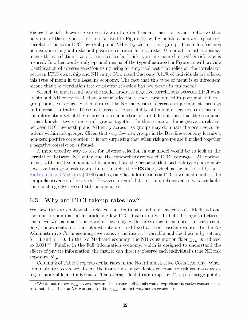
Figure 1 which shows the various types of optimal menus that can occur. Observe thatonly one of these types, the one displayed in Figure 1e, will generate a non-zero (positive)correlation between LTCI ownership and NH entry within a risk group. This menu featuresno insurance for good risks and positive insurance for bad risks. Under all the other optimalmenus the correlation is zero because either both risk-types are insured or neither risk-type isinsured. In other words, only optimal menus of the type illustrated in Figure 1e will provideidentification of adverse selection using using an empirical test that relies on the correlationbetween LTCI ownership and NH entry. Now recall that only 0.11% of individuals are offeredthis type of menu in the Baseline economy. The fact that this type of menu is so infrequentmeans that the correlation test of adverse selection has low power in our model.

Second, to understand how the model produces negative correlations between LTCI own-ership and NH entry recall that adverse selection is more pronounced in poor and frail riskgroups and, consequently, denial rates, like NH entry rates, decrease in permanent earningsand increase in frailty. These facts create the possibility of finding a negative correlation ifthe information set of the insurer and econometrician are different such that the econome-trician bunches two or more risk groups together. In this scenario, the negative correlationbetween LTCI ownership and NH entry across risk groups may dominate the positive corre-lations within risk groups. Given that very few risk groups in the Baseline economy feature anon-zero positive correlation, it is not surprising that when risk groups are bunched togethera negative correlation is found.

A more effective way to test for adverse selection in our model would be to look at thecorrelation between NH entry and the comprehensiveness of LTCI coverage. All optimalmenus with positive amounts of insurance have the property that bad-risk types have morecoverage than good risk types. Unfortunately, the HRS data, which is the data used by bothFinkelstein and McGarry (2006) and us, only has information on LTCI ownership, not on thecomprehensiveness of coverage. However, even if data on comprehensiveness was available,the bunching effect would still be operative.

6.3 Why are LTCI takeup rates low?

We now turn to analyze the relative contributions of administrative costs, Medicaid andasymmetric information in producing low LTCI takeup rates. To help distinguish betweenthem, we will compare the Baseline economy with three other economies. In each econ-omy, endowments and the interest rate are held fixed at their baseline values. In the NoAdministrative Costs economy, we remove the insurer’s variable and fixed costs by settingλ = 1 and γ = 0. In the No Medicaid economy, the NH consumption floor cNH is reducedto 0.001.55 Finally, in the Full Information economy, which is designed to understand theeffects of private information, the insurer can directly observe each individual’s true NH riskexposure, θif,w.

Column 2 of Table 6 reports denial rates in the No Administrative Costs economy. Whenadministrative costs are absent, the insurer no longer denies coverage to risk groups consist-ing of more affluent individuals. The average denial rate drops by 51.4 percentage points.

55We do not reduce cNH to zero because then some individuals would experience negative consumption.Also note that the non-NH consumption floor, co, does not vary across economies.

32

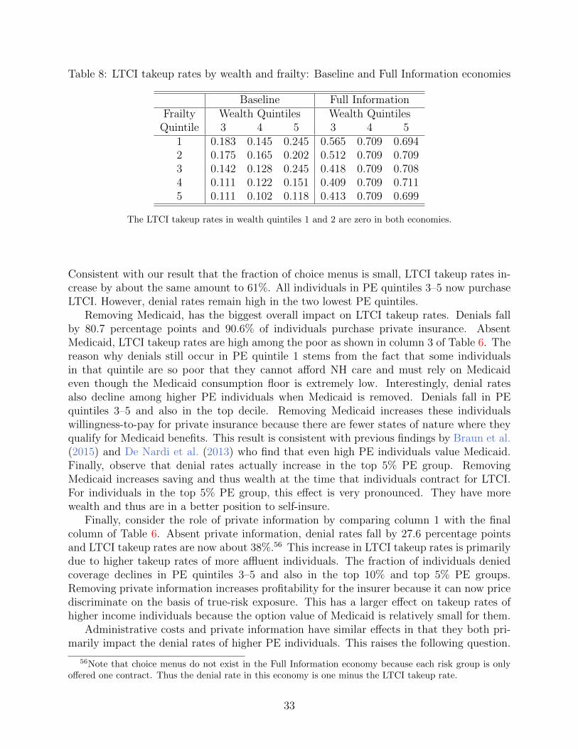
Table 8: LTCI takeup rates by wealth and frailty: Baseline and Full Information economies

Baseline Full InformationFrailty Wealth Quintiles Wealth Quintiles

Quintile 3 4 5 3 4 51 0.183 0.145 0.245 0.565 0.709 0.6942 0.175 0.165 0.202 0.512 0.709 0.7093 0.142 0.128 0.245 0.418 0.709 0.7084 0.111 0.122 0.151 0.409 0.709 0.7115 0.111 0.102 0.118 0.413 0.709 0.699

The LTCI takeup rates in wealth quintiles 1 and 2 are zero in both economies.

Consistent with our result that the fraction of choice menus is small, LTCI takeup rates in-crease by about the same amount to 61%. All individuals in PE quintiles 3–5 now purchaseLTCI. However, denial rates remain high in the two lowest PE quintiles.

Removing Medicaid, has the biggest overall impact on LTCI takeup rates. Denials fallby 80.7 percentage points and 90.6% of individuals purchase private insurance. AbsentMedicaid, LTCI takeup rates are high among the poor as shown in column 3 of Table 6. Thereason why denials still occur in PE quintile 1 stems from the fact that some individualsin that quintile are so poor that they cannot afford NH care and must rely on Medicaideven though the Medicaid consumption floor is extremely low. Interestingly, denial ratesalso decline among higher PE individuals when Medicaid is removed. Denials fall in PEquintiles 3–5 and also in the top decile. Removing Medicaid increases these individualswillingness-to-pay for private insurance because there are fewer states of nature where theyqualify for Medicaid benefits. This result is consistent with previous findings by Braun et al.(2015) and De Nardi et al. (2013) who find that even high PE individuals value Medicaid.Finally, observe that denial rates actually increase in the top 5% PE group. RemovingMedicaid increases saving and thus wealth at the time that individuals contract for LTCI.For individuals in the top 5% PE group, this effect is very pronounced. They have morewealth and thus are in a better position to self-insure.

Finally, consider the role of private information by comparing column 1 with the finalcolumn of Table 6. Absent private information, denial rates fall by 27.6 percentage pointsand LTCI takeup rates are now about 38%.56 This increase in LTCI takeup rates is primarilydue to higher takeup rates of more affluent individuals. The fraction of individuals deniedcoverage declines in PE quintiles 3–5 and also in the top 10% and top 5% PE groups.Removing private information increases profitability for the insurer because it can now pricediscriminate on the basis of true-risk exposure. This has a larger effect on takeup rates ofhigher income individuals because the option value of Medicaid is relatively small for them.

Administrative costs and private information have similar effects in that they both pri-marily impact the denial rates of higher PE individuals. This raises the following question.

56Note that choice menus do not exist in the Full Information economy because each risk group is onlyoffered one contract. Thus the denial rate in this economy is one minus the LTCI takeup rate.

33

Is private information essential to generate the extent and pattern of denials, and henceLTCI takeup, observed in the data or could the model do just as well if we abstracted fromit? Table 8 reports LTCI takeup rates in the Baseline and Full Information economies. Thetable shows that, not only does the presence of private information reduce the extent of LTCItakeup, but it also plays an important and unique role in allowing the model to account forthe empirical pattern of LTCI takeup among affluent individuals. Notice that, in wealthquintiles 4 and 5 of the Full Information economy, the LTCI takeup rates exhibit the wrongpattern by frailty (see also Table 2). LTCI takeup rates in these two wealth quintiles aredeclining in frailty in the data and the Baseline economy. However, in the Full Informa-tion economy, they are constant in frailty in wealth quintile 4 and hump-shaped in frailtyin quintile 5. As we discuss in Section 6.5, even if we reparametrize the Full Informationeconomy, it is unable to match both the level and pattern of LTCI takeup in the data. Thesefindings show that the extent and pattern of private information in the market documentedby Finkelstein and McGarry (2006) and Hendren (2013) is an important driver of low LTCItakeup rates and their correlation with frailty.

In the Baseline economy, like in the U.S., a substantial fraction of NH costs are paidfor out-of-pocket. There are two reasons for this. First, as we explained in Section 4, veryfew NH residents have both LTCI and Medicaid, and LTCI contracts only provide partialcoverage. Second, many individuals who do not purchase LTCI are too affluent to qualityfor Medicaid NH benefits and have no recourse but to pay for their NH care out-of-pocket.The bottom two rows of Table 6 report statistics related to this second source of out-of-pocket payments. In these two rows, individuals in the model who are denied coverageby the insurer are divided into two groups: those who, if they survive to the very old ageand enter a NH, would qualify for Medicaid NH benefits and those who would not. In thebaseline economy, 42.5% of individuals denied coverage would be completely uninsured, ifthey enter a NH, because they would be too affluent to satisfy the Medicaid means test. Thisgroup pays all of their NH expenses out-of-pocket. Notice that the insurance coverage gapdecreases substantially if either administrative costs or private information is absent. In theNo Administrative Cost economy, only 1.6% of those who are denied coverage would end uppaying for all their care out-of-pocket and, in the Full Information economy, only 18.6% ofindividuals would find themselves in this situation. The reason the coverage gap is so smallin these two economies is because denial rates are much lower among high PE individuals.Thus most high PE individuals are covered by private LTCI, while less affluent individualscontinue to receive extensive Medicaid coverage. These findings indicate that policies aimedat correcting supply-side distortions in the U.S. LTCI market could lead to large reductionsin the fraction of individuals paying out-of-pocket for NH care.

6.4 Coverage, loads and profits

We now turn to consider the individual roles of Medicaid, administrative costs and privateinformation in determining the pricing and comprehensiveness of coverage in insurable riskgroups.

Table 9 reports the LTCI takeup rates, fractions of NH costs covered, and loads ongood and bad-risk types in the Baseline economy and the other three economies. The tablereports the average value of each statistic and and a break down by private information type.

34

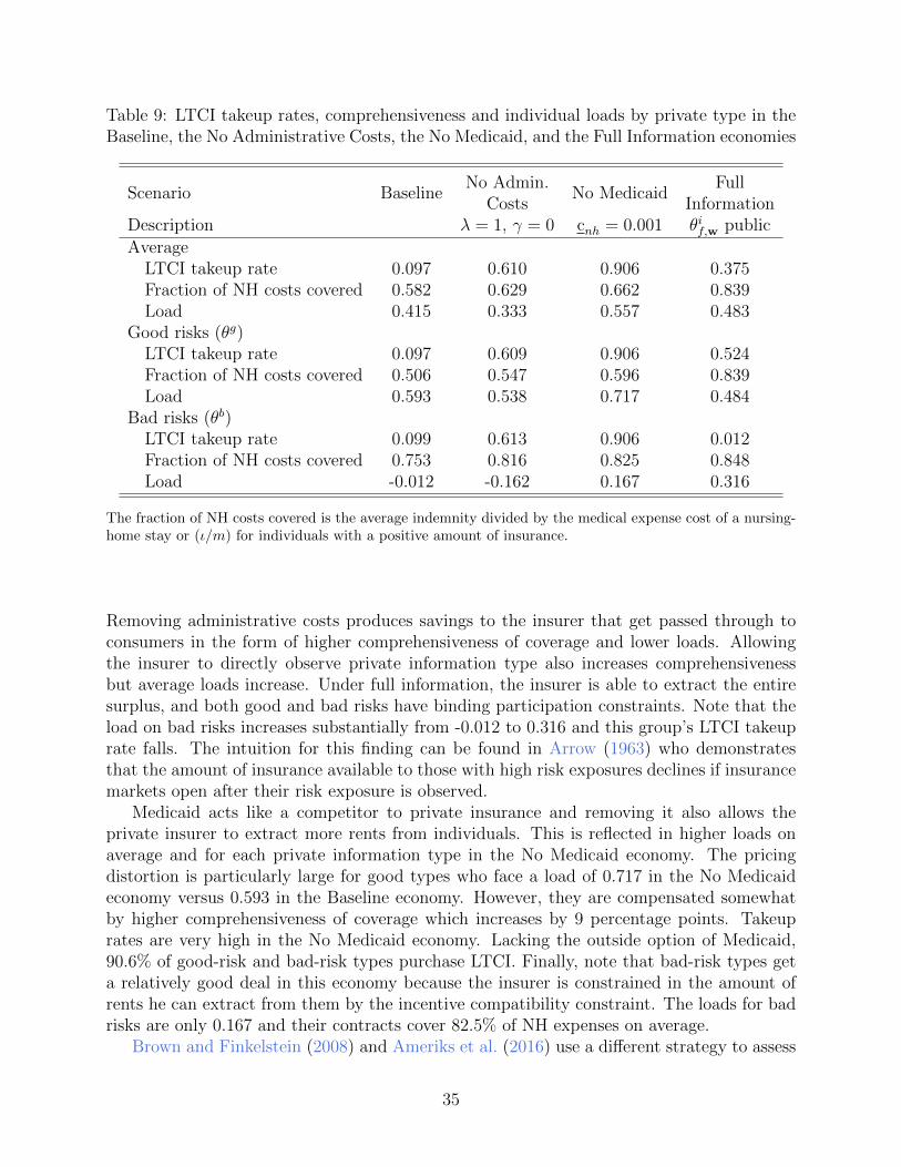
Table 9: LTCI takeup rates, comprehensiveness and individual loads by private type in theBaseline, the No Administrative Costs, the No Medicaid, and the Full Information economies

Scenario BaselineNo Admin.

No MedicaidFull

Costs InformationDescription λ = 1, γ = 0 cnh = 0.001 θif,w public

AverageLTCI takeup rate 0.097 0.610 0.906 0.375Fraction of NH costs covered 0.582 0.629 0.662 0.839Load 0.415 0.333 0.557 0.483

Good risks (θg)LTCI takeup rate 0.097 0.609 0.906 0.524Fraction of NH costs covered 0.506 0.547 0.596 0.839Load 0.593 0.538 0.717 0.484

Bad risks (θb)LTCI takeup rate 0.099 0.613 0.906 0.012Fraction of NH costs covered 0.753 0.816 0.825 0.848Load -0.012 -0.162 0.167 0.316

The fraction of NH costs covered is the average indemnity divided by the medical expense cost of a nursing-home stay or (ι/m) for individuals with a positive amount of insurance.

Removing administrative costs produces savings to the insurer that get passed through toconsumers in the form of higher comprehensiveness of coverage and lower loads. Allowingthe insurer to directly observe private information type also increases comprehensivenessbut average loads increase. Under full information, the insurer is able to extract the entiresurplus, and both good and bad risks have binding participation constraints. Note that theload on bad risks increases substantially from -0.012 to 0.316 and this group’s LTCI takeuprate falls. The intuition for this finding can be found in Arrow (1963) who demonstratesthat the amount of insurance available to those with high risk exposures declines if insurancemarkets open after their risk exposure is observed.

Medicaid acts like a competitor to private insurance and removing it also allows theprivate insurer to extract more rents from individuals. This is reflected in higher loads onaverage and for each private information type in the No Medicaid economy. The pricingdistortion is particularly large for good types who face a load of 0.717 in the No Medicaideconomy versus 0.593 in the Baseline economy. However, they are compensated somewhatby higher comprehensiveness of coverage which increases by 9 percentage points. Takeuprates are very high in the No Medicaid economy. Lacking the outside option of Medicaid,90.6% of good-risk and bad-risk types purchase LTCI. Finally, note that bad-risk types geta relatively good deal in this economy because the insurer is constrained in the amount ofrents he can extract from them by the incentive compatibility constraint. The loads for badrisks are only 0.167 and their contracts cover 82.5% of NH expenses on average.

Brown and Finkelstein (2008) and Ameriks et al. (2016) use a different strategy to assess

35

Table 10: LTCI takeup rates, comprehensiveness, and individual loads in the economy withno private information and no administrative costs.

Wealth Quintile1 2 3 4 5

LTCI takeup rates 0.00 0.04 1.00 1.00 1.00Fraction of loss covered NA 0.50 0.61 0.88 0.97Average load NA 0.16 0.30 0.41 0.38

Frailty Quintile1 2 3 4 5

LTCI takeup rates 0.75 0.67 0.62 0.57 0.44Fraction of loss covered 0.85 0.83 0.80 0.77 0.80Average load 0.42 0.42 0.41 0.40 0.43

NA denotes cases where the denominator is zero.

the roles of high loads, incomplete coverage and Medicaid in accounting for low LTCI takeuprates. Both of these papers specify contracts exogenously and consider counterfactuals inwhich individuals are offered full insurance against NH risk at an actuarially-fair price.Brown and Finkelstein (2008) find that only the top one-third of individuals, when rankedby wealth, purchase a full-coverage actuarially-fair LTCI policy when Medicaid is present.In other words, in their model Medicaid crowds-out the demand for LTCI by individuals inthe bottom two-thirds of the wealth distribution. In our model contracts are endogenousand the insurer responds to Medicaid not only by adjusting the fraction of individuals whoit insures but also by adjusting the comprehensiveness and pricing of the contracts.

As we now show, the crowding-out effect of Medicaid is much smaller when the insurer’soptimal contracting problem is modeled. To illustrate this point, consider a version ofour Baseline economy in which the two supply-side frictions — private information andadministrative costs — are removed. Medicaid is present with the consumption floor set atthe baseline level. Insurance is not actuarially fair in this scenario, the average load is 0.36,due to the fact that the insurer is a monopolist. Nevertheless, 61% of individuals purchaseLTCI. Table 10 reports LTCI takeup rates, comprehensiveness of coverage and average loadsby wealth and frailty quintiles in this alternative economy. LTCI takeup rates are 100% inwealth quintiles 3–5. Medicaid crowds out most private insurance in wealth quintile 2 andall private insurance in quintile 1. Wealth quintile 2 is particularly interesting because theload on insurance for this group is only 0.16 and thus reasonably close to the actuarially-fairbenchmark. Yet, LTCI only covers half of the loss. These individuals are not interested ina full-coverage private LTCI product because for some values of the demand shock they willqualify for Medicaid NH benefits.57 Indeed, 96% of individuals in wealth quintile 2 prefer torely exclusively on Medicaid.

Coverage levels are higher in the top two wealth quintiles. Individuals in quintile 4 receiveextensive coverage (88% of the loss) and those in quintile 5 receive nearly full coverage withinsurance covering 97% of the loss. For the latter group, the chance of receiving Medicaid

57Recall that the optimal contracts have this same partial coverage property in the simple model.

36

NH benefits is particularly low and full coverage is attractive to them. This final propertyof the model is related to Ameriks et al. (2016). They find that 66% of individuals in asample of affluent individuals with median wealth of $543,000 have demand for an idealstate-contingent LTCI product that is priced in an actuarially-fair manner. However, only22% of their respondents hold LTCI and they refer to this as a “LTCI puzzle.” For purposesof comparison, in our baseline model, average wealth in wealth quintile 5 is $695,000 andaverage wealth in quintile 4 is $304,000.58 In our baseline economy, individuals in wealthquintiles 4–5 have LTCI takeup rates of 14% and 21%, respectively. Thus, we find that theLTCI puzzle that Ameriks et al. (2016) document for wealthy individuals can be attributedto supply-side distortions induced by private information and administrative costs.

We have focused on these two examples because they are the most relevant to our analysis.However, it is common practice in the literature to abstract from the contract design problemof the insurer when modeling the LTCI market. Some recent examples include Lockwood(2016) who analyzes optimal saving and bequests in a setting with exogenously specifiedLTCI and Mommaerts (2015) and Ko (2016) who analyze the informal care market underthe assumption that an alternative option is an exogenously specified LTCI contract. Itis conceivable that modeling the supply-side of the LTCI market would also provide newinsights into saving decisions of the old in the presence of bequest motives and demand forinformal care.

6.4.1 Profits

In Section 2 we documented that profits in the U.S. private LTCI market are low. Profitsare also low in our Baseline economy. They are 2.3% of revenues. The left panel of Figure 7,which reports the distribution of profits by frailty and PE quintiles in the Baseline economy,reveals that most profits come from insuring healthy rich individuals as most of the otherrisk groups are denied coverage and profits are thus zero. Medicaid, administrative costs andprivate information all work to reduce profits. Medicaid, however, has the largest impact.When it is removed profits rise to 28.5% of revenues.59 The right panel of Figure 7 showsthe distribution of profits by frailty and PE quintiles in the No Medicaid economy. In thiseconomy, in contrast to the Baseline, the insurer generates most of his profits from the poor.Profits fall monotonically with permanent earnings and do not vary as much with frailty.Medicaid has a large effect on profits for two reasons. First, Medicaid’s presence dramaticallyreduces the fraction of insurable risk groups. When Medicaid is removed the fraction ofinsurable risk groups increases sharply. Second, as we explained above in the discussion ofloads, Medicaid also substantially lowers profit margins in insurable risk groups.

6.5 Robustness

We start by considering the robustness of our finding that optimal menus that feature choiceare rare. The parameter ψ plays a central role in determining the costs of cross-subsidizationfrom good to bad-risk types and ultimately the fraction of risk groups that are offered

58Both figures are expressed in terms of year 2000 dollars.59Profits are 15.2% of revenues in the No Administrative Costs economy and 9.8% of revenues in the Full

Information economy.

37

1 2 3 4 5Frailty quintile

0

10

20

30

40

50

Sha

re o

f tot

al p

rofit

s (%

)PE quintile 1PE quintile 2PE quintile 3PE quintile 4PE quintile 5

1 2 3 4 5Frailty quintile

0

2

4

6

8

10

12

14

Sha

re o

f tot

al p

rofit

s (%

)

PE quintile 1PE quintile 2PE quintile 3PE quintile 4PE quintile 5

Figure 7: Profits Baseline and No Medicaid Specifications.The left (right) panel reports the distribution of profits by frailty and PE quintiles in the Baseline (No

Medicaid) economy. Note the difference in scale of the two plots.

an optimal menu that provides them with the choice of either positive insurance or noinsurance. In our setting with a monopoly insurer, premia from good types are used tocross-subsidize premia for bad types. If ψ is reduced a smaller fraction of good types isavailable to provide the subsidies and it becomes more likely that the optimal menus ininsurable risk groups include a (0, 0) contract. To explore the quantitative significance ofthis effect, we reparametrized the model with ψ reduced from its baseline value of 0.709 to0.609. When ψ is 0.609 the fraction of individuals that are offered the choice of a (0, 0)contract and opt for it increases from 0.11% to 6.3% and the number of denials falls to 82%.Even though choice becomes relatively more important, risk-group selection is still the mainreason why LTCI takeup rates are low. One important difference between this scenario andthe baseline parametrization is that it is much easier to detect adverse selection by comparingNH entry frequencies of LTCI holders and non-holders in this scenario. For instance, thefraction of LTCI holders who enter a NH (conditional on survival) is now larger, at 0.44,than the fraction of non-holders who enter a NH (0.40). Thus, the model with a lower valueof ψ no longer accounts for the adverse selection correlation puzzle.

Another important difference is that the model with the lower value of ψ exhibits toolittle dispersion in private information as compared to our data. The coefficient of variationof private information produced by the model falls from 0.94 in the baseline to 0.86 whenψ = 0.609. Recall, that the target for our baseline value of ψ is the coefficient of variationof self-reported NH entrance probabilities. Our data measure omits responses of 0, 1/2 and1. If some/all of these responses are included, the coefficient of variation for self-reportedNH risk is even larger than 0.94. In this sense, our strategy for setting ψ in the baselineparametrization is conservative. Apart from these two differences, the performance of themodel with a lower ψ is similar to our baseline parametrization. In particular, this versionof the model is able to match the pattern of LTCI takeup rates and NH entry rates by frailtyand wealth.

Our strategy for parametrizing the model used particular data facts to pin down thescale of Medicaid NH benefits and administrative costs. We have explored how the resultschange if we assign a more prominent role to each of these factors. One experiment we have

38

performed is to increase the scale of the Medicaid consumption floor by a factor of 1.76.This value lies at the upper end of values used in previous studies.60 Private informationand administrative costs continue to have a large impact on LTCI takeup rates of affluentindividuals even with the higher consumption floor. For instance, LTCI takeup rates increaseby 50% or more if the private information distortion is removed.

Recall that LTCI takeup rates are very high in the Full Information economy. We havealso investigated whether it is possible to reparametrize this version of the model to reproducethe LTCI takeup rates in the data. We need significantly higher administrative costs (49%of premia instead of 33%) to get the average takeup rate to match the data. However, thisparametrization cannot generate the empirical pattern of LTCI takeup rates at alternativefrailty quintiles among more affluent individuals no matter how we adjust the NH entryprobability distribution.

In addition, we have considered how well the model performs if it is reparametrizedunder the assumption that administrative costs are absent. This version of the model failsto produce low LTCI takeup rates among affluent risk-groups with high frailty levels. Forinstance, the model predicts that LTCI takeup rates of individuals in wealth and frailtyquintile 5 are nearly 1 while they are only 0.1 in our data. More complete details aboutthese robustness checks can be found in Section 5.2 of the appendix.

Finally, our finding that adverse selection is an important factor is robust to the level ofrisk aversion. We set σ to 2 but there is not a consensus in the profession on its value andlarger values have been used by others in the insurance literature. For instance, Amerikset al. (2011) use a value of 3. Under our parameterization scheme, if we used a higher valueof σ, adverse selection would play a bigger role in accounting for low LTCI takeup rates.The easiest way to see this is to consider the simple model described in Section 3. For givenchoices of the parameters that determine the administrative costs and the scale of Medicaid (λ ,γ, and cNH), a higher value of risk aversion requires more dispersion in private informationor a higher fraction of bad-types to produce the same level of takeup rates.

Our model has abstracted from several features of the U.S. LTCI market. Most notablyin recent years regulators in this industry have required that insurers add markups, called“pricing margins”, to the price of their initial premia to reduce the probability of futurepremium increases due to intertemporal risk. We do not model pricing margins. In themodel neither individuals nor the insurer face aggregate uncertainty about interest rates,mortality rates or LTCI takeup rates and there is no reason to provision for it. Pricingmargins could compound the problem of adverse selection.

We have also abstracted from moral hazard. In the 1980s and early 1990s LTC insurerswere not concerned about moral hazard because they felt that individuals given the choicewould prefer not to be institutionalized. However, as coverage has been expanded to providehome care benefits, insurers have had to allocate more resources to claims managementto ascertain that individuals have an ongoing need for LTC services. In this sense, highadministrative costs in this market may partially reflect moral hazard.

60See Kopecky and Koreshkova (2014) for a summary of previous studies.

39

7 Concluding Remarks

We have found that Medicaid, administrative costs and adverse selection all play importantbut distinct roles in accounting for the observation that LTCI takeup rates are low at allwealth levels and decline with health status. Modeling these three factors also allowed usto account for a broad range of other empirical features of this market including coveragelevels and pricing of insurance, low profitability, and the low empirical correlation betweenLTCI ownership and nursing home entry.

Our result that risk-group selection is a quantitatively important screening device maybe relevant in other insurance markets. For instance, the U.S. individual health insurancemarket prior to the Affordable Care Act (ACA) shared many features with the U.S. LTCImarket: takeup rates were low, denials were common, and loads were high for insured in-dividuals. Underwriting is also used as a screening device in life and disability insurancemarkets.

References

Ameriks, J., J. Briggs, A. Caplin, M. Shapiro, and C. Tonetti (2016): “Late-in-Life Risks and the Under-Insurance Puzzle,” Working Paper.

Ameriks, J., A. Caplin, S. Laufer, and S. Van Nieuwerburgh (2011): “The Joy ofGiving or Assisted Living? Using Strategic Surveys to Separate Bequest and PrecautionaryMotives,” Journal of Finance, 66, 519–561.

Arrow, K. (1963): “Uncertainty and the Welfare Economics of Medical Care,” AmericanEconomic Review, 53, 941–973.

Braun, R. A., K. Kopecky, and T. Koreshkova (2015): “Old, Sick, Alone andPoor: A Welfare Analysis of Old-Age Social Insurance Programs,” Forthcoming Reviewof Economic Studies.

Brown, J. R. and A. Finkelstein (2007): “Why is the Market for Long-Term CareInsurance So Small?” Journal of Public Economics, 91, 1967–1991.

——— (2008): “The Interaction of Public and Private Insurance: Medicaid and the Long-Term Care Insurance Market,” American Economic Review, 98, 1083–1102.

——— (2011): “Insuring Long-Term Care in the United States,” Journal of Economic Per-spectives, 25, 119–42.

Chade, H. and E. Schlee (2016): “Insurance as a Lemons Market: Coverage Denialsand Pooling,” Working Paper.

Chiappori, P.-A. and B. Salanie (2000): “Testing for Asymmetric Information in In-surance Markets,” Journal of Political Economy, 108, 56–78.

40

Cohen, M., R. Kaur, and D. B. (2013): “Exiting the Market: Understanding the factorsbehind carriers’ decision to leave the long-term care insurance market,” , U.S. Departmentof Health and Human Services and Thomson Reuters.

Cutler, D. (1996): “Why don’t markets insure long-term risk?” Working Paper.

De Nardi, M., E. French, and J. B. Jones (2013): “Medicaid Insurance in Old Age,”Working Paper.

Eaton, R. (2016): “Long-Term Care Insurance: The SOA Pricing Project,” Society ofActuaries.

Fang, H., M. A. Keane, and D. Silverman (2008): “Sources of Advantageous Selection:Evidence from the Medigap Insurance Market,” Journal of Political Economy, 116, 303–350.

Favreault, M. and J. Dey (2016): “Long-Term Services and Supports for Older Ameri-cans: Risks and Financing,” Tech. rep., U.S. Department of Health and Human Services.

Finkelstein, A. and K. McGarry (2006): “Multiple Dimensions of Private Information:Evidence from the Long-Term Care Insurance Market,” American Economic Review, 96,938–958.

Harris-Kojetin, L., E. Park-Lee, et al. (2016): “Long-term care proviers and servicesusers in the United States: Data from the National Study of Long-Term Care Providers,2013-2014,” National Center for Health Statistics. Vital Health Stat, 3.

Hendren, N. (2013): “Private Information and Insurance Rejections,” Econometrica, 81,1713–1762.

Hendricks, L. (2001): “Bequests and Retirement Wealth in the United States,” .

Hurd, M., P. Michaud, and S. Rohwedder (2013): “The Lifetime Risk of NursingHome Use,” Working Paper.

Karaca-Mandic, P., J. Abraham, and C. Phelps (2011): “How do health insur-ance loading fees vary by group size?: Implications for Healthcare reform,” InternationalJournal of Health Care Finance and Economics, 11, 181–207.

Ko, A. (2016): “An Equilibrium Analysis of the Long-Term Care Insurance Market,” Un-published.

Kopecky, K. and T. Koreshkova (2014): “The Impact of Medical and Nursing HomeExpenses on Savings,” American Economic Journal: Macroeconomics, 6, 29–72.

Lester, B., A. Shourideh, V. Venkateswaran, and A. Zetlin-Jones (2015):“Screening and Adverse Selection in Frictional Markets,” Working Paper.

Lewis, S., J. Wilkin, and M. Merlis (2003): “Regulation of Private Long-Term Care

41

Insurance: Implmentation Experience and Key Issues,” Tech. rep., Henry J. Kaiser FamilyFoundation.

Lockwood, L. (2016): “Incidental Bequests: Bequest Motives and the Choice to Self-InsureLate-Life Risks,” Working paper.

Mahoney, N. (2015): “Bankruptcy as Implicit Health Insurance,” American EconomicReview, 105, 710–46.

Mitchell, O. S., J. M. Poterba, M. J. Warshawsky, and J. R. Brown (1999):“New Evidence on the Money’s Worth of Individual Annuities,” American Economic Re-view, 89, 1299–1318.

Mommaerts, C. (2015): “Long-term Care Insurance and the Family,” Unpublished.

Murtaugh, C. M., P. Kemper, B. C. Spillman, and B. L. Carlson (1997): “TheAmount, Distribution, and Timing of Lifetime Nursing Home Use,” Medical Care, 35,204–218.

Poterba, J. M., S. F. Venti, and D. A. Wise (2011): “Family Status Transitions,Latent Health, and the Post-Retirement Evolution of Assets,” in Explorations in the Eco-nomics of Aging, University of Chicago Press.ed. D. Wise, University of Chicago Press:D. Wise.

Purcell, P. J. (2012): “Income replacement ratios in the Health and Retirement Study,”Social Security Bulletin, 72, 37.

Rothschild, M. and J. Stiglitz (1976): “Equilibrium in Competitive Insurance Mar-kets: An Essay on the Economics of Imperfect Information,” The Quarterly Journal ofEconomics, 90, 629–649.

Spillman, B. and K. Black (2015): “The Size of the Long-Term Care Population inResidential Care: A Review of Estimates and Methodology,” Tech. rep.

Stiglitz, J. (1977): “Non-Linear Pricing and Imperfect Information: The Insurance Mar-ket,” The Review of Economic Studies, 44, 407–430.

Thau, C., D. Helwig, and A. Schmitz (2014): “2014 Long Term Care Insurance Sur-vey,” Broker World.

42