olevel additional mathematics revision notes
TRANSCRIPT
OLEVEL ADDITIONAL MATHEMATICS REVISION NOTESOLEVEL ADDITIONAL MATHEMATICS REVISION NOTESOLEVEL ADDITIONAL MATHEMATICS REVISION NOTESOLEVEL ADDITIONAL MATHEMATICS REVISION NOTES
Compiled by: FAHMEED RAJPUTCompiled by: FAHMEED RAJPUTCompiled by: FAHMEED RAJPUTCompiled by: FAHMEED RAJPUT
Chartered Accountant, Petroleum Engr.Chartered Accountant, Petroleum Engr.Chartered Accountant, Petroleum Engr.Chartered Accountant, Petroleum Engr.
MBA, M.PhilMBA, M.PhilMBA, M.PhilMBA, M.Phil
Tables and MatricesTables and MatricesTables and MatricesTables and Matrices
Tables of values may often be naturally represented as matrices, and operations performed on them.
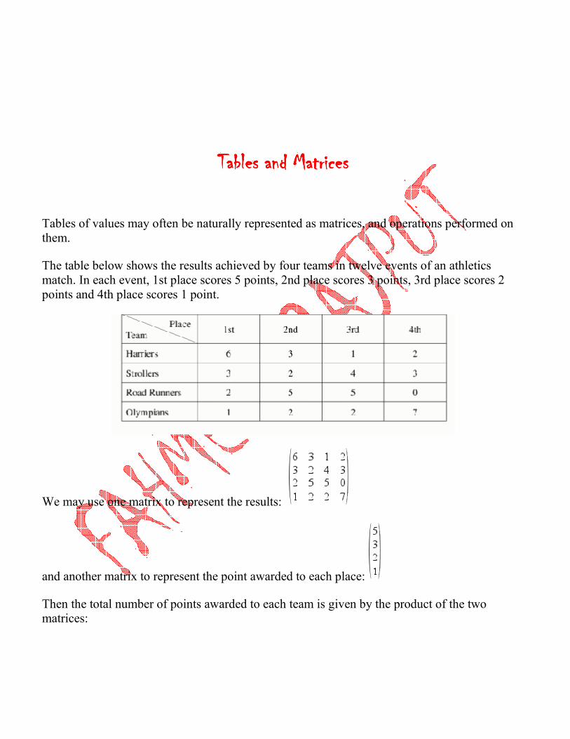
The table below shows the results achieved by four teams in twelve events of an athletics match. In each event, 1st place scores 5 points, 2nd place scores 3 points, 3rd place scores 2 points and 4th place scores 1 point.
We may use one matrix to represent the results:
and another matrix to represent the point awarded to each place:
Then the total number of points awarded to each team is given by the product of the two matrices:
This is possible because the places in the table occupy the columns and the place values in the column vectors occupy the rows. When we multiply as above we sum the total points for each team.
This method is applicable to a wide variety of situations and suitable for calculation by computers. It is widely used in spreadsheets.
Amplitude, Period, Maximum and Minimum of Trigonometric FunctionsAmplitude, Period, Maximum and Minimum of Trigonometric FunctionsAmplitude, Period, Maximum and Minimum of Trigonometric FunctionsAmplitude, Period, Maximum and Minimum of Trigonometric Functions
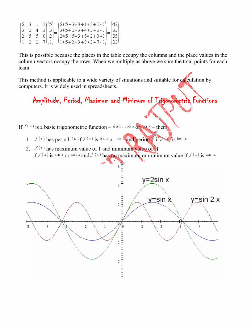
If is a basic trigonometric function – or – then
1. has period if is or and period if is
2. has maximum value of 1 and minimum value of -1 if is or and has no maximum or minimum value if is
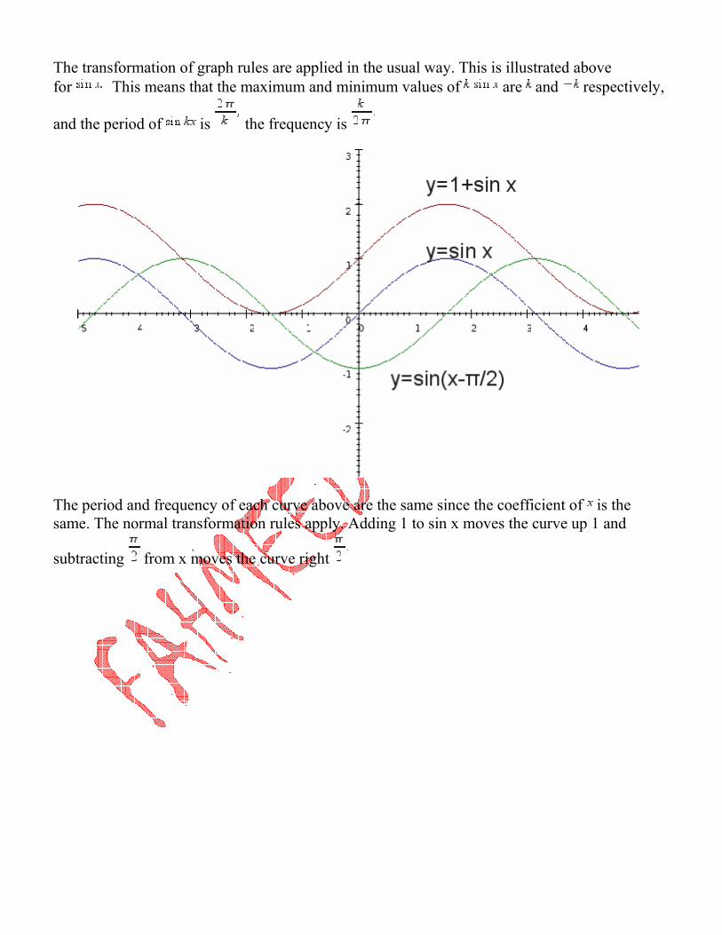
The transformation of graph rules are applied in the usual way. This is illustrated above for This means that the maximum and minimum values of are and respectively,
and the period of is the frequency is
The period and frequency of each curve above are the same since the coefficient of is the same. The normal transformation rules apply. Adding 1 to sin x moves the curve up 1 and
subtracting from x moves the curve right
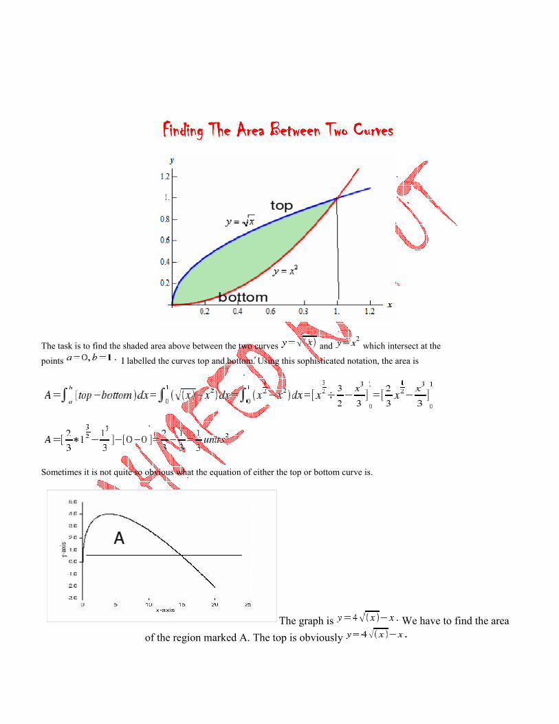
Finding The Area Between Two CurvesFinding The Area Between Two CurvesFinding The Area Between Two CurvesFinding The Area Between Two Curves
The task is to find the shaded area above between the two curves and which intersect at the
points I labelled the curves top and bottom. Using this sophisticated notation, the area is
Sometimes it is not quite so obvious what the equation of either the top or bottom curve is.
The graph is We have to find the area
of the region marked A. The top is obviously
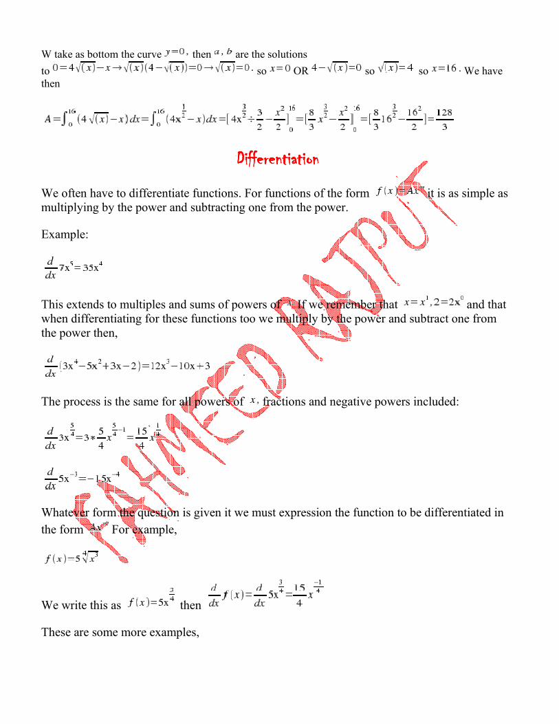
W take as bottom the curve then are the solutions
to so OR so so We have then
DifferentiationDifferentiationDifferentiationDifferentiation
We often have to differentiate functions. For functions of the form it is as simple as multiplying by the power and subtracting one from the power.
Example:
This extends to multiples and sums of powers of If we remember that and that when differentiating for these functions too we multiply by the power and subtract one from the power then,
The process is the same for all powers of fractions and negative powers included:
Whatever form the question is given it we must expression the function to be differentiated in the form For example,
We write this as then
These are some more examples,
Differentiation is used to find rates of change (when we differentiate with respect to time), gradients, slopes, tangents and normals.
Maxima and Minima Maxima and Minima Maxima and Minima Maxima and Minima –––– The Second Differential CriterionThe Second Differential CriterionThe Second Differential CriterionThe Second Differential Criterion
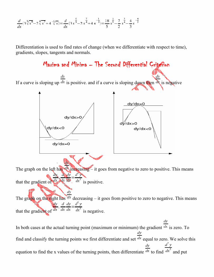
If a curve is sloping up is positive. and if a curve is sloping down then is negative
The graph on the left has increasing – it goes from negative to zero to positive. This means
that the gradient of is positive.
The graph on the right has decreasing – it goes from positive to zero to negative. This means
that the gradient of is negative.
In both cases at the actual turning point (maximum or minimum) the gradient is zero. To
find and classify the turning points we first differentiate and set equal to zero. We solve this
equation to find the x values of the turning points, then differentiate to find and put
the values we have found into this expression. If the value we obtain here is positive then we have found a minimum for If the value we obtain is negative then we have found a maximum for If we need to find the – coordinate too we can substitute the – values of the minimum into the original expression for
To summarise:
To find a turning point solve for
To classify a turning point, put the values of the turning point into the expression for
If this value is positive, we have a minimum, and if it is negative we have a maximum. To find the – value of the turning point, substitute the – values of the turning point into the expression for
Example. Find and classify the turning points of
Solve
so the coordinates of the turning point are
Therefore this is a minimum.
Example. Find and classify the turning points of
Solve
When
When
At therefore this is a minimum.
At therefore this is a maximum.
2 x 2 Matrices 2 x 2 Matrices 2 x 2 Matrices 2 x 2 Matrices –––– Sums, Products DetSums, Products DetSums, Products DetSums, Products Determinants and Inverseserminants and Inverseserminants and Inverseserminants and Inverses
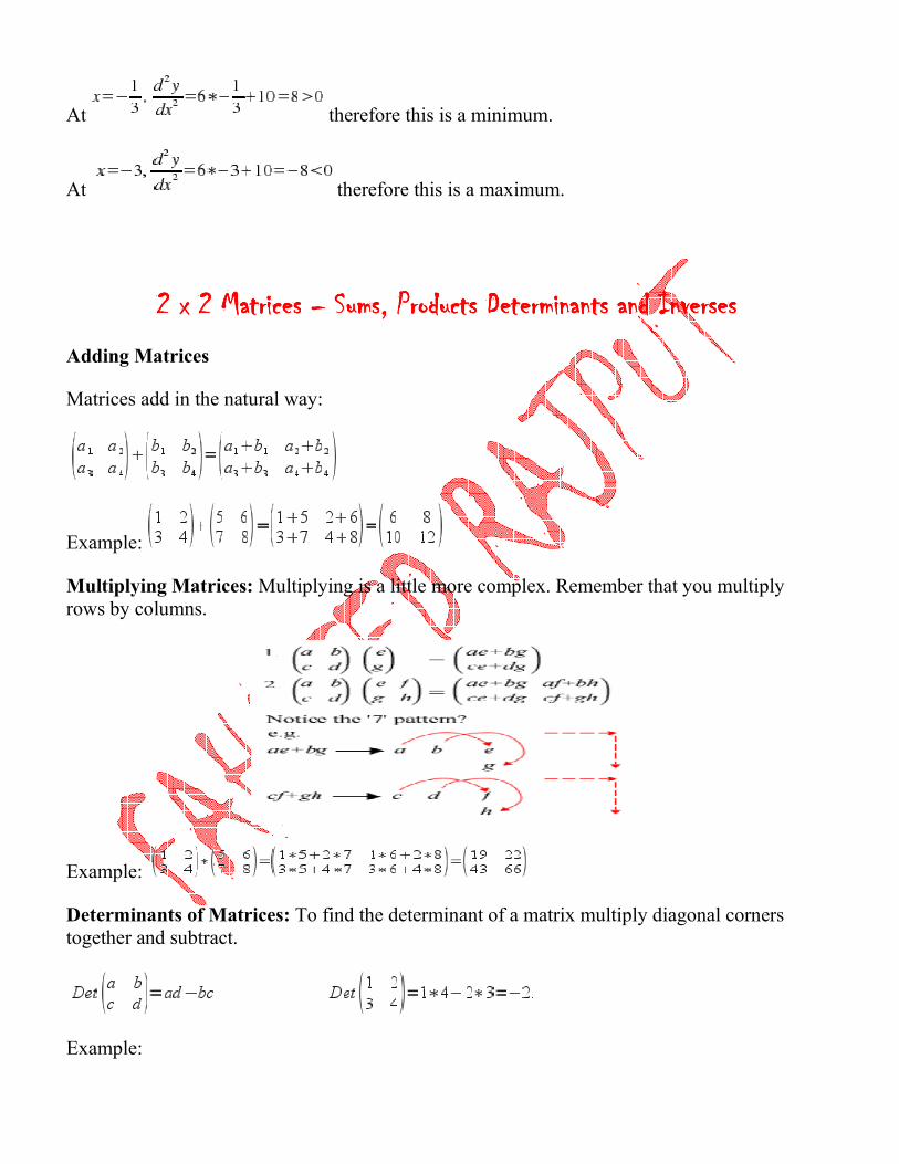
Adding Matrices
Matrices add in the natural way:
Example:
Multiplying Matrices: Multiplying is a little more complex. Remember that you multiply rows by columns.
Example:
Determinants of Matrices: To find the determinant of a matrix multiply diagonal corners together and subtract.
Example:
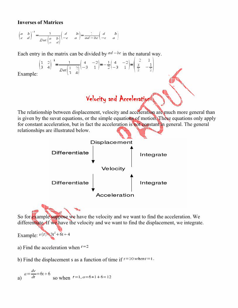
Inverses of Matrices
Each entry in the matrix can be divided by in the natural way.
Example:
Velocity and AccelerationVelocity and AccelerationVelocity and AccelerationVelocity and Acceleration
The relationship between displacement, velocity and acceleration are much more general than is given by the suvat equations, or the simple equations of motion. These equations only apply for constant acceleration, but in fact the acceleration is not constant in general. The general relationships are illustrated below.
So for example suppose we have the velocity and we want to find the acceleration. We differentiate. If we have the velocity and we want to find the displacement, we integrate.
Example:
a) Find the acceleration when
b) Find the displacement s as a function of time if
a) so when
b}
We are told that when so
The BinomThe BinomThe BinomThe Binomial Expansion.ial Expansion.ial Expansion.ial Expansion. The binomial Theorem allows us to expand many brackets without multiplying each bracket out one by one. It states:
To expand we could expand which would be a very long winded process. Or we could just substitute for and into the expression for the binomial expansion. Example: Expand then
which simplifies to
and further to
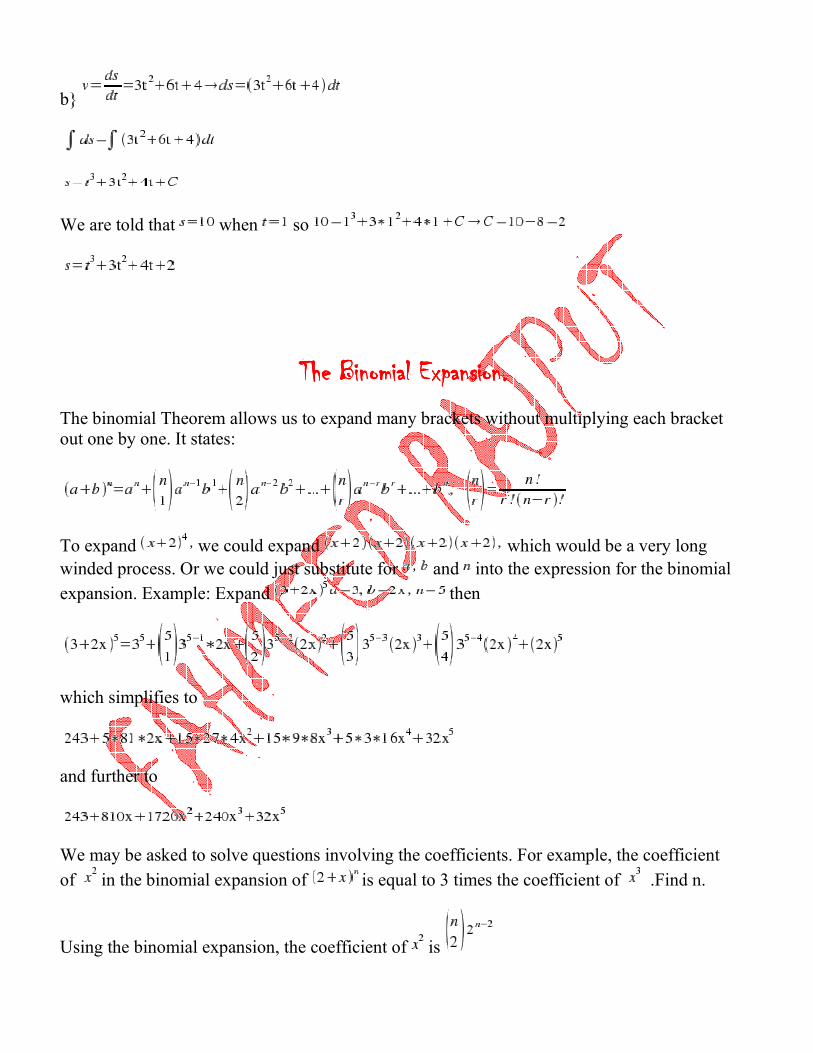
We may be asked to solve questions involving the coefficients. For example, the coefficient of in the binomial expansion of is equal to 3 times the coefficient of .Find n.
Using the binomial expansion, the coefficient of is
Using the binomial expansion, the coefficient of is
Hence we can write down the equation
Now we have to perform some trickery:
Practical VectorsPractical VectorsPractical VectorsPractical Vectors
Planes rarely fly in the direction they are pointing. If the wind is blowing and the world is turning the pilot has to take account of these when he plots a course. Even with modern gps systems available, , it is beneficial to the pilot to take these into account because of the resulting increase in fuel efficiency. It is worse though for the sailor, who has to take the tide into account as well
We can deal with these problems by representing the velocities of the wind, tide and boat as vectors, then using trigonometry to find the course to take or the velocity to travel at.
For example:
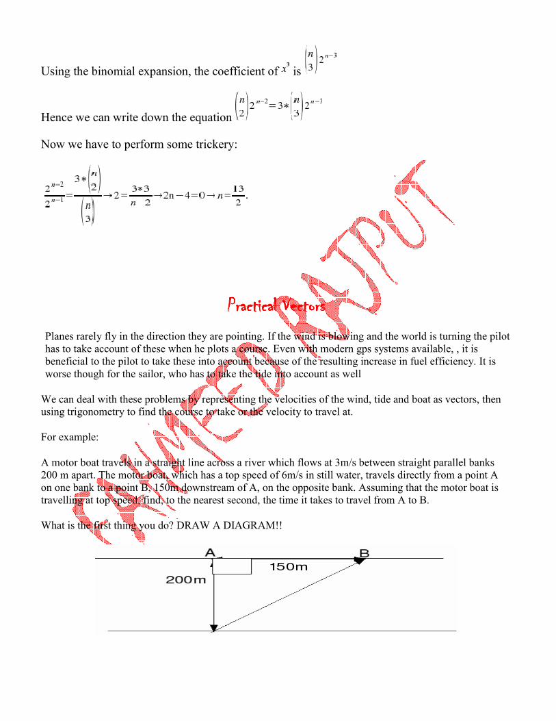
A motor boat travels in a straight line across a river which flows at 3m/s between straight parallel banks 200 m apart. The motor boat, which has a top speed of 6m/s in still water, travels directly from a point A on one bank to a point B, 150m downstream of A, on the opposite bank. Assuming that the motor boat is travelling at top speed, find, to the nearest second, the time it takes to travel from A to B.
What is the first thing you do? DRAW A DIAGRAM!!
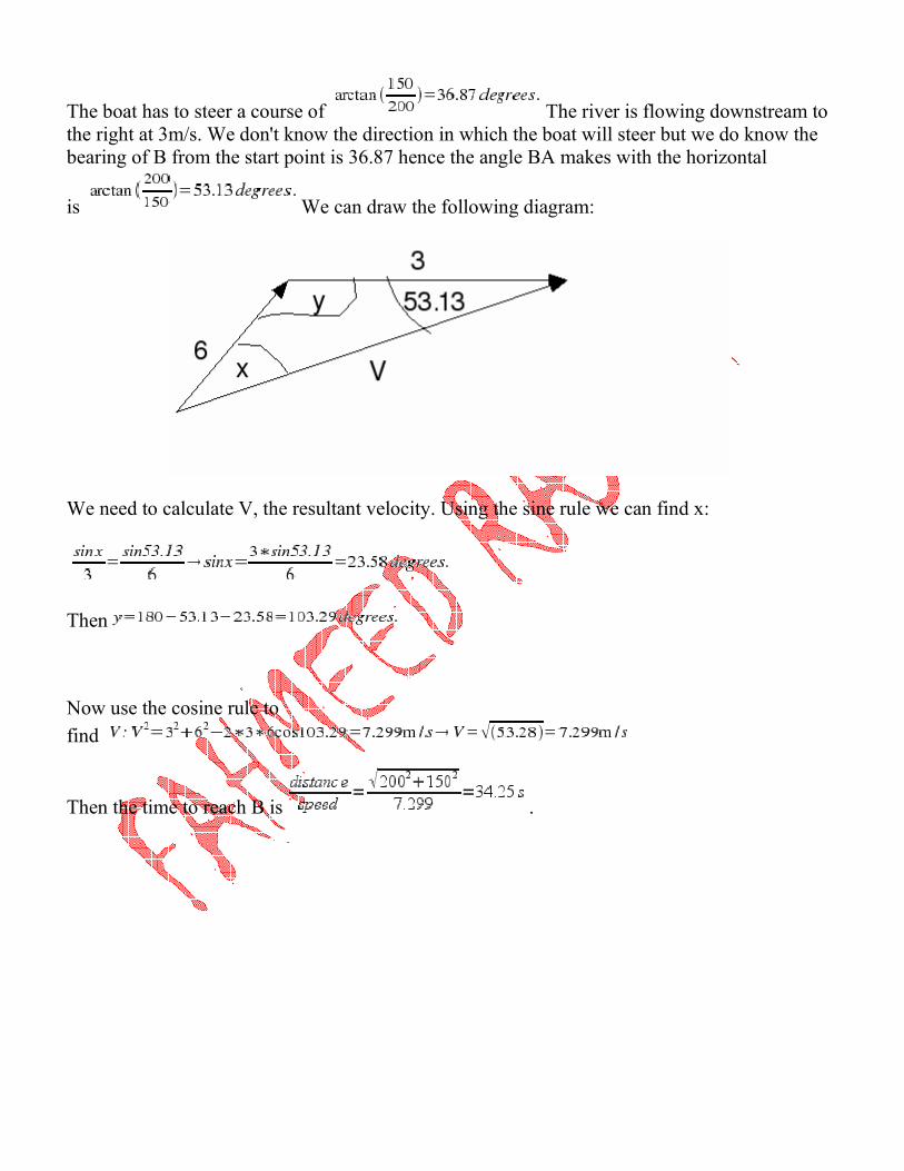
The boat has to steer a course of The river is flowing downstream to the right at 3m/s. We don't know the direction in which the boat will steer but we do know the bearing of B from the start point is 36.87 hence the angle BA makes with the horizontal
is We can draw the following diagram:
We need to calculate V, the resultant velocity. Using the sine rule we can find x:
Then
Now use the cosine rule to find
Then the time to reach B is .
Integration by ParIntegration by ParIntegration by ParIntegration by Partstststs
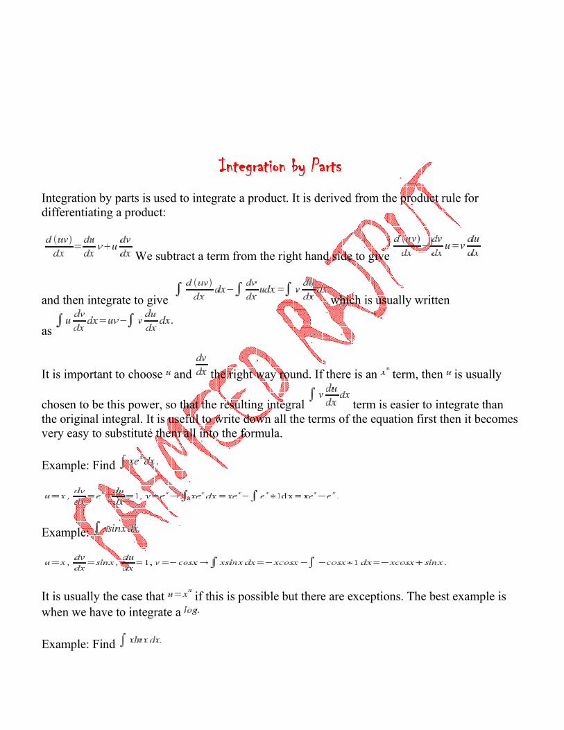
Integration by parts is used to integrate a product. It is derived from the product rule for differentiating a product:
We subtract a term from the right hand side to give
and then integrate to give which is usually written
as
It is important to choose and the right way round. If there is an term, then is usually
chosen to be this power, so that the resulting integral term is easier to integrate than the original integral. It is useful to write down all the terms of the equation first then it becomes very easy to substitute them all into the formula.
Example: Find
Example:
It is usually the case that if this is possible but there are exceptions. The best example is when we have to integrate a
Example: Find
Example: Find
To integrate this we have to write
Maximisation or Optimisation ProblemsMaximisation or Optimisation ProblemsMaximisation or Optimisation ProblemsMaximisation or Optimisation Problems
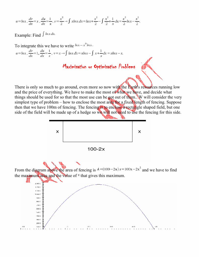
There is only so much to go around, even more so now with the Earth's resources running low and the price of everything. We have to make the most of what we have, and decide what things should be used for so that the most use can be got out of them.. W will consider the very simplest type of problem – how to enclose the most area for a fixed length of fencing. Suppose then that we have 100m of fencing. The fencing is to enclose a rectangle shaped field, but one side of the field will be made up of a hedge so we will not need to use the fencing for this side.
From the diagram above the area of fencing is and we have to find the maximum area and the value of that gives this maximum.
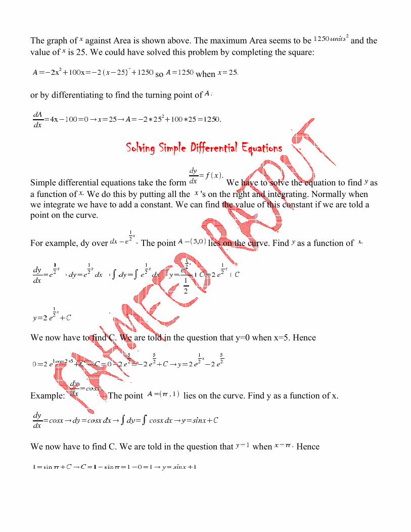
The graph of against Area is shown above. The maximum Area seems to be and the value of is 25. We could have solved this problem by completing the square:
so when
or by differentiating to find the turning point of
Solving Simple Differential EquationsSolving Simple Differential EquationsSolving Simple Differential EquationsSolving Simple Differential Equations
Simple differential equations take the form We have to solve the equation to find as a function of We do this by putting all the 's on the right and integrating. Normally when we integrate we have to add a constant. We can find the value of this constant if we are told a point on the curve.
For example, dy over The point lies on the curve. Find as a function of
We now have to find C. We are told in the question that y=0 when x=5. Hence
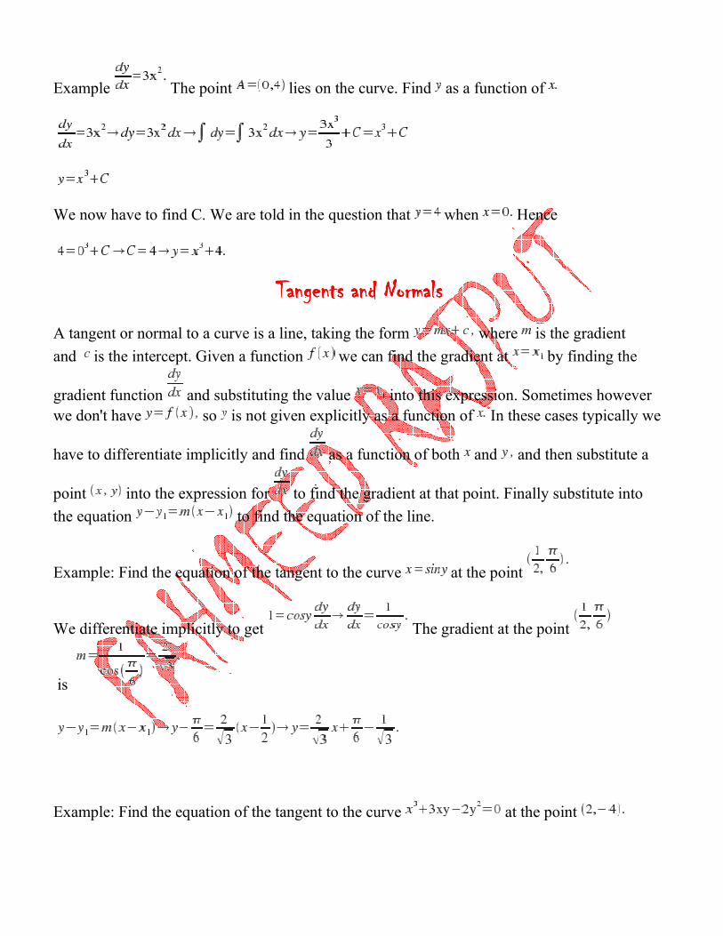
Example: The point lies on the curve. Find y as a function of x.
We now have to find C. We are told in the question that when Hence
Example The point lies on the curve. Find as a function of
We now have to find C. We are told in the question that when Hence
Tangents and NTangents and NTangents and NTangents and Normalsormalsormalsormals
A tangent or normal to a curve is a line, taking the form where is the gradient and is the intercept. Given a function we can find the gradient at by finding the
gradient function and substituting the value into this expression. Sometimes however we don't have so is not given explicitly as a function of In these cases typically we
have to differentiate implicitly and find as a function of both and and then substitute a
point into the expression for to find the gradient at that point. Finally substitute into the equation to find the equation of the line.
Example: Find the equation of the tangent to the curve at the point
We differentiate implicitly to get The gradient at the point
is
Example: Find the equation of the tangent to the curve at the point
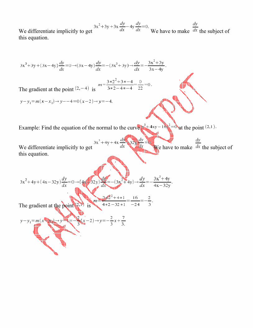
We differentiate implicitly to get We have to make the subject of this equation.
The gradient at the point is
Example: Find the equation of the normal to the curve at the point
We differentiate implicitly to get We have to make the subject of this equation.
The gradient at the point is
Solving Quadratic InequalitiesSolving Quadratic InequalitiesSolving Quadratic InequalitiesSolving Quadratic Inequalities
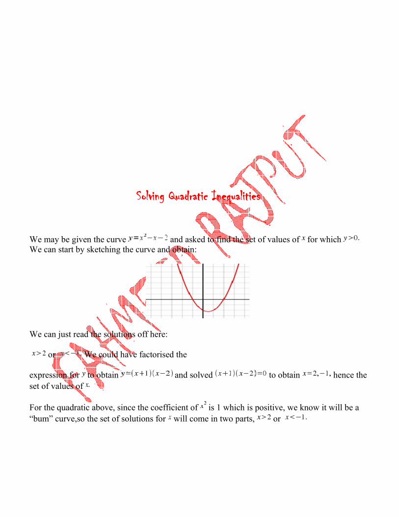
We may be given the curve and asked to find the set of values of for whichWe can start by sketching the curve and obtain:
We can just read the solutions off here:
or We could have factorised the
expression for to obtain and solved to obtain hence the set of values of
For the quadratic above, since the coefficient of is 1 which is positive, we know it will be a “bum” curve,so the set of solutions for will come in two parts, or

The curve shown above is We are asked for example to find the set of values offor which We can see from the graph that there is only one set of values: We could have factorised the expression for to obtain and solved to obtain hence we could write down the set of values of
The curve shown is We are asked
to solve The curve is a “breast” curve and we can read off the solutions or
We can also factorise the expression for to obtain and solve hence finding the set of solutions just given.
The RemaindThe RemaindThe RemaindThe Remainder Theoremer Theoremer Theoremer Theorem
The Remainder Theorem is the generalized form of The Factor Theorem.
The Remainder Theorem
When a polynomial expression is divided by a linear factor the remainder
is If then is a factor of
Example:
Show that is a factor of
therefore is a factor.
Example
If the remainder when is divided by is 3 and the remainder when is divided by is 4, find and
Remainder of on division by is
Remainder when p(x) is divided by is
We solve the simultaneous equations
(1)
(2)
(1)+2*(2) gives then from (2)
Then
Using Straight Line Graphs to Find the Relationship Between Two QuantitiesUsing Straight Line Graphs to Find the Relationship Between Two QuantitiesUsing Straight Line Graphs to Find the Relationship Between Two QuantitiesUsing Straight Line Graphs to Find the Relationship Between Two Quantities
A linear relationship is the easiest relationship to decode ie. find a relationship for. It may be that even if two quantities are not in a linear relationship, functions of the quantities can be found that do bear a linear relationship. We may then plot graphs of the functions, and if the relationship appears linear we may write down a linear relationship between the two functions over the range of observations.
In attempting to find a straight line relationship we may try logarithmic, reciprocal or power relationships. We can plot products of powers of and against logs of functions of and We are looking to obtain a straight line relationship. Towards this end we make the following observations:
If the graph curves up the taking or a root of – or equivalently, exponentiating or raising to some power – will tend to straighten the curve out, but often some foresight is needed. There is a positive relationship between and in the table below,
0.100 0.125 0.160 0.200 0.400
0.050 0.064 0.085 0.111 0.286
since both increase together, but the relationship is not linear since the gradient between
is not the same as
for
We can take the reciprocals of both and and plot against The transformed data is
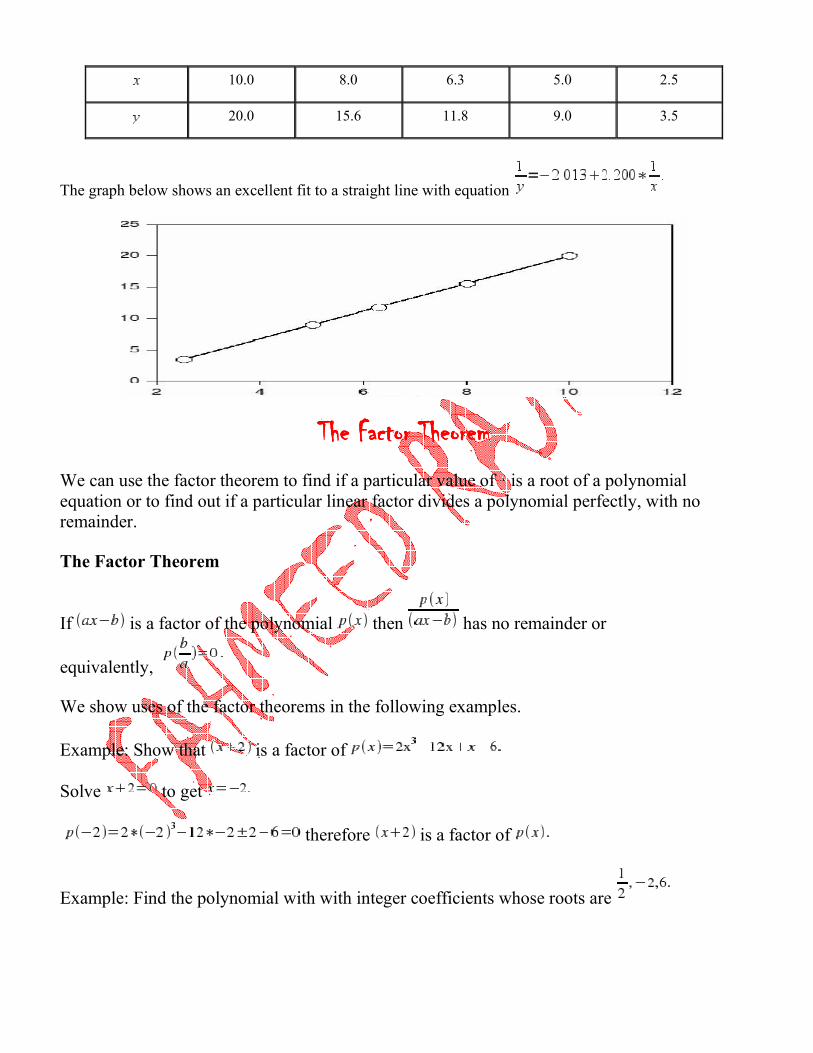
10.0 8.0 6.3 5.0 2.5
20.0 15.6 11.8 9.0 3.5
The graph below shows an excellent fit to a straight line with equation
The Factor TheoremThe Factor TheoremThe Factor TheoremThe Factor Theorem
We can use the factor theorem to find if a particular value of is a root of a polynomial equation or to find out if a particular linear factor divides a polynomial perfectly, with no remainder.
The Factor Theorem
If is a factor of the polynomial then has no remainder or
equivalently,
We show uses of the factor theorems in the following examples.
Example: Show that is a factor of
Solve to get
therefore is a factor of
Example: Find the polynomial with with integer coefficients whose roots are
If these are the roots, the factors are or or and hence we expand and simplify to get #
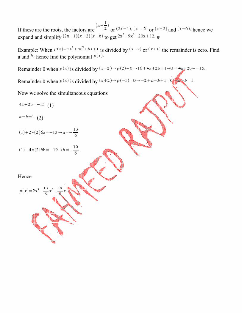
Example: When is divided by or the remainder is zero. Find a and hence find the polynomial
Remainder 0 when is divided by
Remainder 0 when is divided by
Now we solve the simultaneous equations
(1)
(2)
Hence
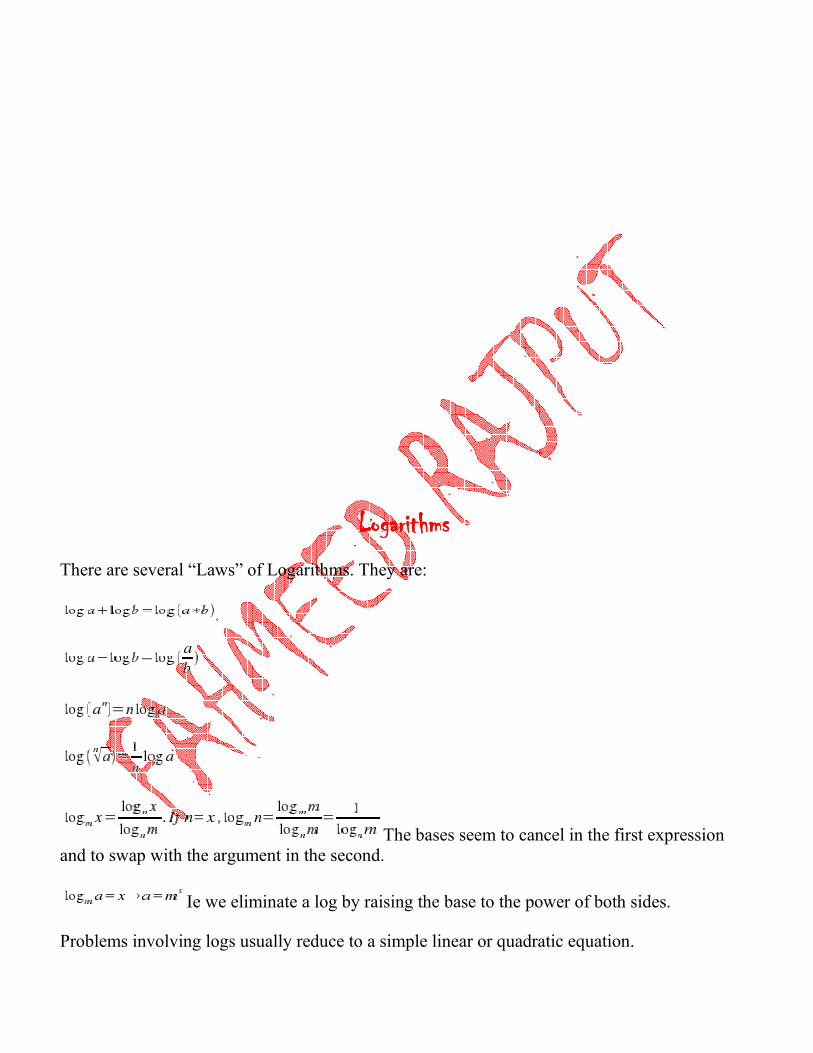
LogarithmsLogarithmsLogarithmsLogarithms
There are several “Laws” of Logarithms. They are:
The bases seem to cancel in the first expression and to swap with the argument in the second.
Ie we eliminate a log by raising the base to the power of both sides.
Problems involving logs usually reduce to a simple linear or quadratic equation.
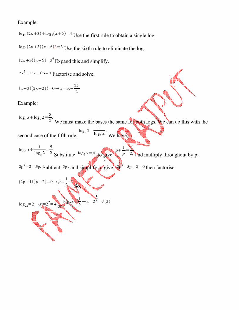
Example:
Use the first rule to obtain a single log.
Use the sixth rule to eliminate the log.
Expand this and simplify.
Factorise and solve.
Example:
We must make the bases the same for both logs. We can do this with the
second case of the fifth rule: We have,
Substitute to give and multiply throughout by p:
Subtract and simplify to give, then factorise.
So,
or
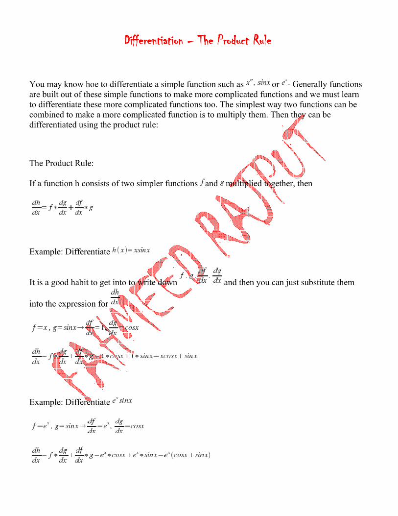
Differentiation Differentiation Differentiation Differentiation –––– The Product RuleThe Product RuleThe Product RuleThe Product Rule
You may know hoe to differentiate a simple function such as or Generally functions are built out of these simple functions to make more complicated functions and we must learn to differentiate these more complicated functions too. The simplest way two functions can be combined to make a more complicated function is to multiply them. Then they can be differentiated using the product rule:
The Product Rule:
If a function h consists of two simpler functions and multiplied together, then
Example: Differentiate
It is a good habit to get into to write down and then you can just substitute them
into the expression for
Example: Differentiate
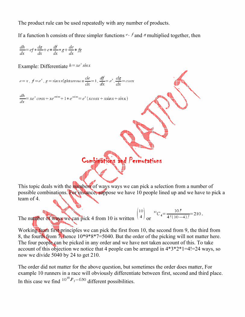
The product rule can be used repeatedly with any number of products.
If a function h consists of three simpler functions and multiplied together, then
Example: Differentiate
Combinations and PermutationsCombinations and PermutationsCombinations and PermutationsCombinations and Permutations
This topic deals with the numbers of ways ways we can pick a selection from a number of possible combinations. For instance, suppose we have 10 people lined up and we have to pick a team of 4.
The number of ways we can pick 4 from 10 is written or
Working from first principles we can pick the first from 10, the second from 9, the third from 8, the fourth from 7, hence 10*9*8*7=5040. But the order of the picking will not matter here. The four people can be picked in any order and we have not taken account of this. To take account of this objection we notice that 4 people can be arranged in 4*3*2*1=4!=24 ways, so now we divide 5040 by 24 to get 210.
The order did not matter for the above question, but sometimes the order does matter, For example 10 runners in a race will obviously differentiate between first, second and third place.
In this case we find different possibilities.
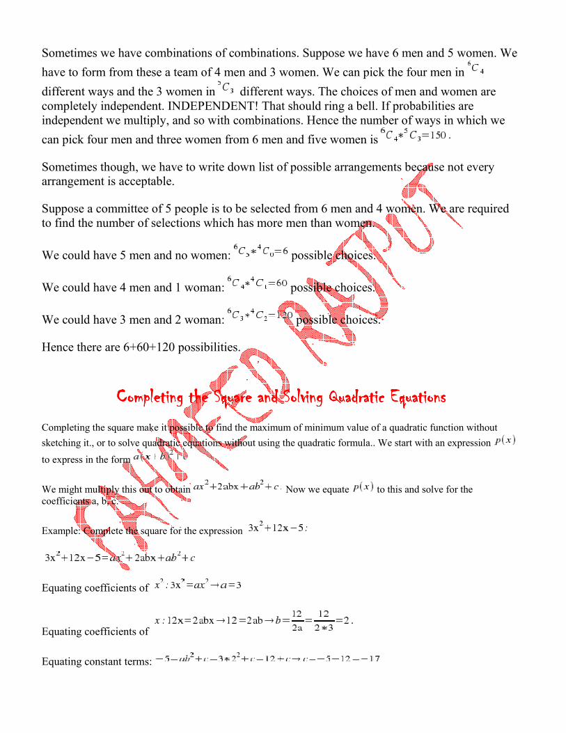
Sometimes we have combinations of combinations. Suppose we have 6 men and 5 women. We
have to form from these a team of 4 men and 3 women. We can pick the four men in
different ways and the 3 women in different ways. The choices of men and women are completely independent. INDEPENDENT! That should ring a bell. If probabilities are independent we multiply, and so with combinations. Hence the number of ways in which we
can pick four men and three women from 6 men and five women is
Sometimes though, we have to write down list of possible arrangements because not every arrangement is acceptable.
Suppose a committee of 5 people is to be selected from 6 men and 4 women. We are required to find the number of selections which has more men than women.
We could have 5 men and no women: possible choices.
We could have 4 men and 1 woman: possible choices.
We could have 3 men and 2 woman: possible choices.
Hence there are 6+60+120 possibilities.
Completing the Square and Solving Quadratic EquationsCompleting the Square and Solving Quadratic EquationsCompleting the Square and Solving Quadratic EquationsCompleting the Square and Solving Quadratic Equations
Completing the square make it possible to find the maximum of minimum value of a quadratic function without
sketching it., or to solve quadratic equations without using the quadratic formula.. We start with an expression
to express in the form
We might multiply this out to obtain Now we equate to this and solve for the coefficients a, b, c.
Example: Complete the square for the expression
Equating coefficients of
Equating coefficients of
Equating constant terms:
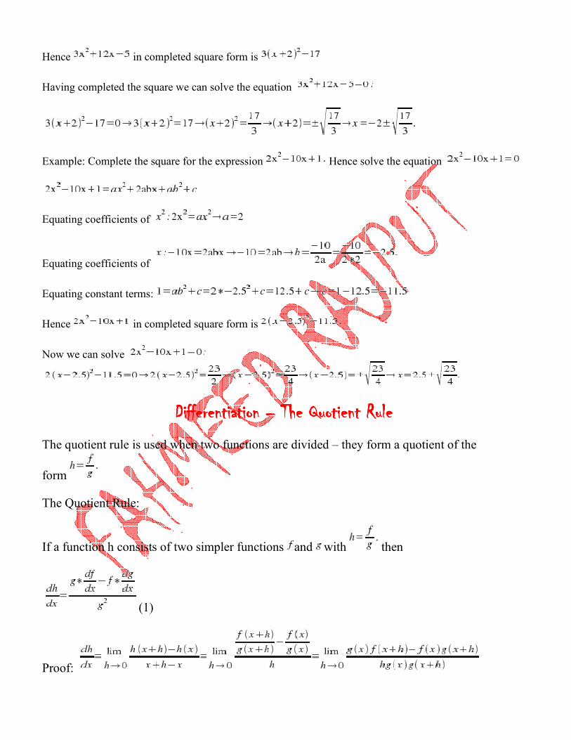
Hence in completed square form is
Having completed the square we can solve the equation
Example: Complete the square for the expression Hence solve the equation
Equating coefficients of
Equating coefficients of
Equating constant terms:
Hence in completed square form is
Now we can solve
Differentiation Differentiation Differentiation Differentiation –––– The Quotient RuleThe Quotient RuleThe Quotient RuleThe Quotient Rule
The quotient rule is used when two functions are divided – they form a quotient of the
form
The Quotient Rule:
If a function h consists of two simpler functions and with then
(1)
Proof:
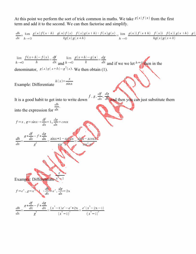
At this point we perform the sort of trick common in maths. We take from the first term and add it to the second. We can then factorise and simplify.
and and if we we let then in the denominator, We then obtain (1).
Example: Differentiate
It is a good habit to get into to write down and then you can just substitute them
into the expression for
Example: Differentiate
Solving Absolute Value EquationsSolving Absolute Value EquationsSolving Absolute Value EquationsSolving Absolute Value Equations
Most equations of the form have two solutions. If we sketch the graphs of the graphs will cross at two points which will be the solutions to the equations. For the graphs
(blue) and (red)
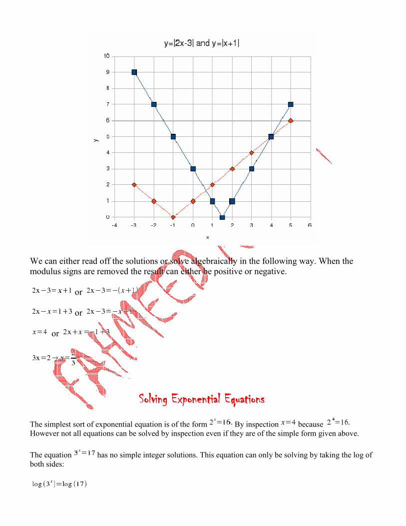
We can either read off the solutions or solve algebraically in the following way. When the modulus signs are removed the result can either be positive or negative.
or
or
or
Solving Exponential EquationsSolving Exponential EquationsSolving Exponential EquationsSolving Exponential Equations
The simplest sort of exponential equation is of the form By inspection because However not all equations can be solved by inspection even if they are of the simple form given above.
The equation has no simple integer solutions. This equation can only be solving by taking the log of both sides:
and then using the power rule for logs:
to 4 significant figures.
Slightly more complicated are expressions where is a power on both sides, for example,
We log both sides to get
Rearrangement of this expression gives
Now we can factorise this expression with x as a common factor on the left hand side to give
to 4 decimal places.
Sometimes an equation may have to be rearranged to express it in one of the above forms. For
example, We use the rule
Then we can log both sides as above
As before we rearrange this equation to make x the subject: to 3 significant figures.
Solving Quadratic Exponential Equations by SubstitutionSolving Quadratic Exponential Equations by SubstitutionSolving Quadratic Exponential Equations by SubstitutionSolving Quadratic Exponential Equations by Substitution
Some exponential equations can be factorised in linear factors. The simplest can be factorised into quadratic equations. We then put each factor equal to zero and solve it.
Example: Solve (1)
Factorise to get
or
The above equation has two solutions. In general, as for quadratic equations, an exponential which can be expressed as two factors can have one, two or no solutions. It is convenient to make clear the connection by expressing the original equation as a quadratic using the substitution Then and equation (1) above becomes This equation factorises to give so Since the original equation was expressed in terms of we still have to find but we can use the substitution with the values of that we have found, to find
or
Example: Solve
Substitute to get and factorise this expression to give
This has no solution since there is no real log of a negative number.
Example: Solve
Substitute to get and factorise this expression to give
This has no solution since there is no real log of a negative number. This has no solution since there is no real log of a negative number hence the equation has no solutions.
Solving Trigonometric EquationsSolving Trigonometric EquationsSolving Trigonometric EquationsSolving Trigonometric Equations
The basic and curves are given on the left below and on the right below:
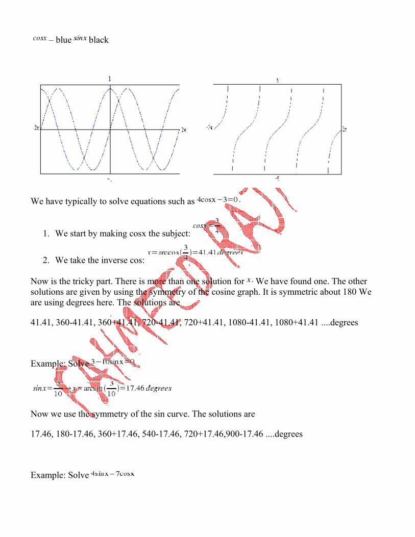
– blue black
We have typically to solve equations such as
1. We start by making cosx the subject:
2. We take the inverse cos:
Now is the tricky part. There is more than one solution for We have found one. The other solutions are given by using the symmetry of the cosine graph. It is symmetric about 180 We are using degrees here. The solutions are
41.41, 360-41.41, 360+41.41, 720-41.41, 720+41.41, 1080-41.41, 1080+41.41 ....degrees
Example: Solve
Now we use the symmetry of the sin curve. The solutions are
17.46, 180-17.46, 360+17.46, 540-17.46, 720+17.46,900-17.46 ....degrees
Example: Solve
Now we we the property of the tan curve that it repeats every 180 degrees. The solutions are
60.26, 180+60.26, 360+60.26, 540+60.26, 720+60.26, 900+60.26.....degrees