OligopolyOutline:

•Salient features of oligopolistic market structures.

•Measures of seller concentration

•Dominant firm oligopoly

•Rivalry among symmetric firms (The Cournot model)

•The kinked demand curve

Oligopoly is a market structure featuring a small number of sellers that together account for a large fraction of market sales.

Oligopoly is derived from the Greek work

“olig” meaning “few” or “a small number.”

Features of oligopoly•Fewness of sellers

•Seller interdependence

•Feasibility of coordinated action among ostensibly independent firms

Measures of seller concentrationThe concentration ratio is the percentage of total market sales accounted for by an absolute number of the largest firms in the market.

The four-firm concentration ratio (CR4) measures the percent of total market sales accounted for by the top four firms in the market.

The eight-firm concentration ratio (CR4) measures the percent of total market sales accounted for by the top eight firms in the market.

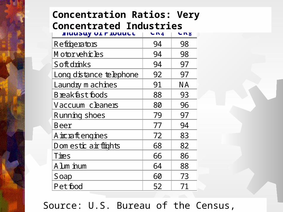
Industry or Product CR4 CR8

Refrigerators 94 98Motor vehicles 94 98Soft drinks 94 97Long distance telephone 92 97Laundry machines 91 NABreakfast foods 88 93Vaccuum cleaners 80 96Running shoes 79 97Beer 77 94Aircraft engines 72 83Domestic air flights 68 82Tires 66 86Aluminum 64 88Soap 60 73Pet food 52 71

Concentration Ratios: Very Concentrated Industries

Source: U.S. Bureau of the Census, Census of Manufacturers

Industry or Product CR4 CR8

Fast food 44 57Personal computers 45 63Office furniture 45 59Toys 41 58Bread 34 47Lawn equipment 40 57Machine tools 30 44Paint 24 36Newspapers 22 34Furniture 17 25Boat building 14 22Concrete 8 12Women's dresses 6 10

Concentration Ratios: Less Concentrated Industries

Source: U.S. Bureau of the Census, Census of Manufacturers

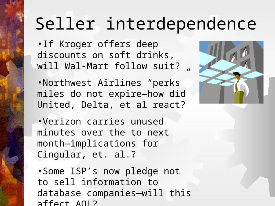
Seller interdependence•If Kroger offers deep discounts on soft drinks, will Wal-Mart follow suit?

•Northwest Airlines “perks” miles do not expire—how did United, Delta, et al react?

•Verizon carries unused minutes over the to next month—implications for Cingular, et. al.?

•Some ISP’s now pledge not to sell information to database companies—will this affect AOL?

•Alcoa’s decision to add production capacity is conditioned upon the investment plans of rival aluminum producers.

Price-Output Determination in Oligopolistic Market Structures

We have good models of price-output determination for the

structural cases of pure competition and pure monopoly. Oligopoly is more problematic,

and a wide range of outcomes is possible.

Dominant firm price leadership

•This is a system of price-output determination we sometimes see in oligopolistic market structures in which there is one firm that is clearly dominant.

•General Motors was once the price leader in the U.S. auto industry.

•Other “dominant” firms include Du Pont in chemicals, US Steel (now USX), Phillip Morris, Fedex, Boeing, General Electric, AT&T, and Hewlett Packard.

The model

The dominant firm sets the market price and remaining firms sell all they wish at this price.

The demand curve for the price leader is found by subtracting the market demand curve from the supply curve of the remaining sellers in the market.

Figure 10.1: Dominant Firm Price Leadership

P'

P*

d Lneader'set demand

Industry demand

Supply curvefor small firms

D

S

d

MC MR

Q* Qs

Dollars per Unit of Output

Output

D

P* is the price established by the dominant firm

Q* + QS

ExampleLet the market demand curve be given by:

QD = 248 – 2P

The supply curve for 10 small firms in the market is given by:

QS = 48 + 3P

The dominant firm’s “residual” or net demand curve is given by the market demand curve minus the supply of the 10 other firms, or:

Q = QD – QS = 248 – 2P – (48 + 3P) = 200 – 5P

The inverse (residual) demand curve facing the dominant firm is given by:

P = 40 - .2Q

Assume the dominant firm has a marginal cost function given by:

MC = .1Q

The dominant firm would maximize its own profits by setting MR = MC. To derive the MR, find the revenue (R) function and take the first derivative with respect to Q:

R = P • Q = (40 - .2Q)Q = 40Q - .2Q2

MR = dR/dQ = 40 - .4Q

Now set MR = MC and solve for Q

40 - .4Q = .1Q.5Q = 40 Q = 80 Units P = 40 – (.2)(80) = $24

At the price established by the dominant firm, the remaining 10 firms collectively supply 120 units (or 12 units each).

Cournot Model1

1 Augustin Cournot. Research Into the Mathematical Principles of the Theory of Wealth, 1838

•Illustrates the principle of mutual interdependence among sellers in tightly concentrated markets--even where such interdependence is unrecognized by sellers.

•Illustrates that social welfare can be improved by the entry of new sellers--even if post-entry structure is oligopolistic.

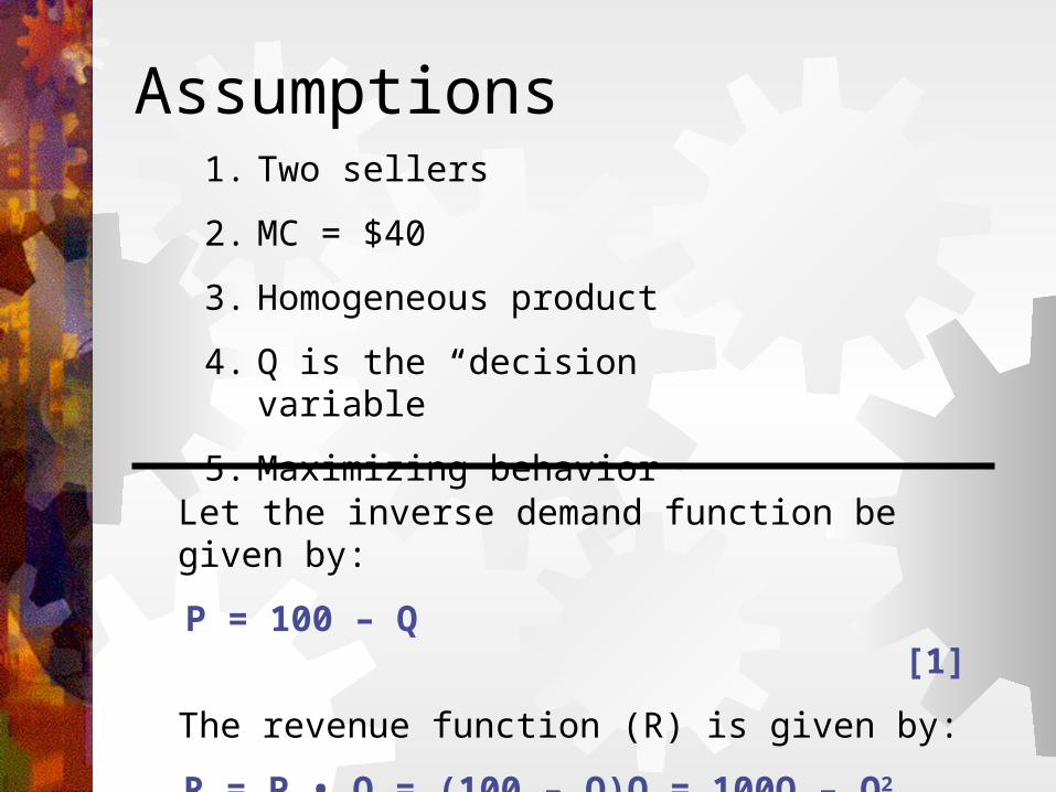
Assumptions1. Two sellers

2. MC = $40

3. Homogeneous product

4. Q is the “decision variable”

5. Maximizing behavior

Let the inverse demand function be given by:

P = 100 – Q [1]

The revenue function (R) is given by:

R = P • Q = (100 – Q)Q = 100Q – Q2 [2]

Thus the marginal revenue (MR) function is given by:

MR = dR/dQ = 100 – 2Q [3]

Let q1 denote the output of seller 1 and q2 is the output of seller 2. Now rewrite equation [1]

P = 100 – q1 – q2 [4]

The profit () functions of sellers 1 and 2 are given by:

1 = (100 – q1 – q2)q1 – 40q1 [5]

2 = (100 – q1 – q2)q2 – 40q2 [6]

Mutual interdependence is revealed by the profit equations. The profits of seller 1 depend

on the output of seller 2—and vice versa

Monopoly caseLet q2 = 0 units so that Q = q1—that is, seller 1 is a monopolist. Seller 1 should set its quantity supplied at the level corresponding to the equality of MR and MC. Let MR – MC = 0

100 – 2Q – 40 = 0

2Q = 60 Q = QM = 30 units

Thus

PM = 100 – QM = $70

Substituting into equation [5], we find that:

= $900

Finding equilibriumQuestion: Suppose that seller 1 expects that seller 2 will supply 10 units. How many units should seller 1 supply based on this expectation?

By equation [4], we can say:

P = 100 – q1 – 10 = 90 – q1 [7]

The the revenue function of seller 1 is given by:

R = P • q1 = (90 – q1)q1 = 90q1 – q12 [8]

Thus:

MR = dR/dq1 = 90 – 2q1 [9]

Subtracting MC from MR

90 – 2q1 – 40 = 0 [10]

2q1 = 50 q1 = 25 units [11]

Thus the profit maximizing output for seller 1, given that q2 = 10 units, is 25 units.

We repeat these calculations for every possible value of q2

and we find that the -maximizing output for seller

1 can be obtained from the following equation:

q1 = 30 - .5q2 [12]

Best reply functionEquation [12] is a best reply function (BRF) for seller 1. It can be used to compute the -maximizing output for seller 1 for any output selected by seller 2.

Output of seller 1

Out

put o

f sel

l er 2

30 - .5q2

60

300

30

10

15 25

In similar fashion, we derive a best reply function for seller 2. It is given by:

q2 = 30 - .5q1 [13]

q1

q2

0

30

60

q2 = 30 - .5q1

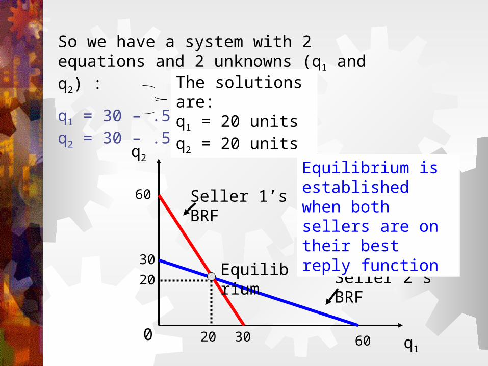
So we have a system with 2 equations and 2 unknowns (q1 and q2) :

q1 = 30 – .5q2

q2 = 30 – .5q1

The solutions are: q1 = 20 units q2 = 20 units

q2

q10

20

20

Equilibrium

Seller 1’s BRF

Seller 2’s BRF

60

30

30 60

Equilibrium is established when both sellers are on their best reply function

Cournot duopoly solution QCOURNOT = 40 Units (20 units each)PCOURNOT = $601 = 2 = $400

Note that:

PCOMPETITIVE = $40QCOMPETITIVE = 60 Units

Therefore

PCOMPETITIVE < PCOURNOT < PMONOPOLY

Implications of the model The Cournot model predicts that, holding elasticity of demand constant, price-cost margins are inversely related to the number of sellers in the marketThis principle is expressed by the following equation

nP

MCP

1)(

[14]

Where is elasticity of demand and n is the number of sellers. So as n , the price-margin approaches zero—as in the purely competitive case.

Theory of 2 demand curves

Sellers in concentrated market structures must form expectations about the likely

reaction of rivals before taking action (for example,

cutting prices).

If I cut my price to $2.49/gallon, what’s the guy down the street

going to do?

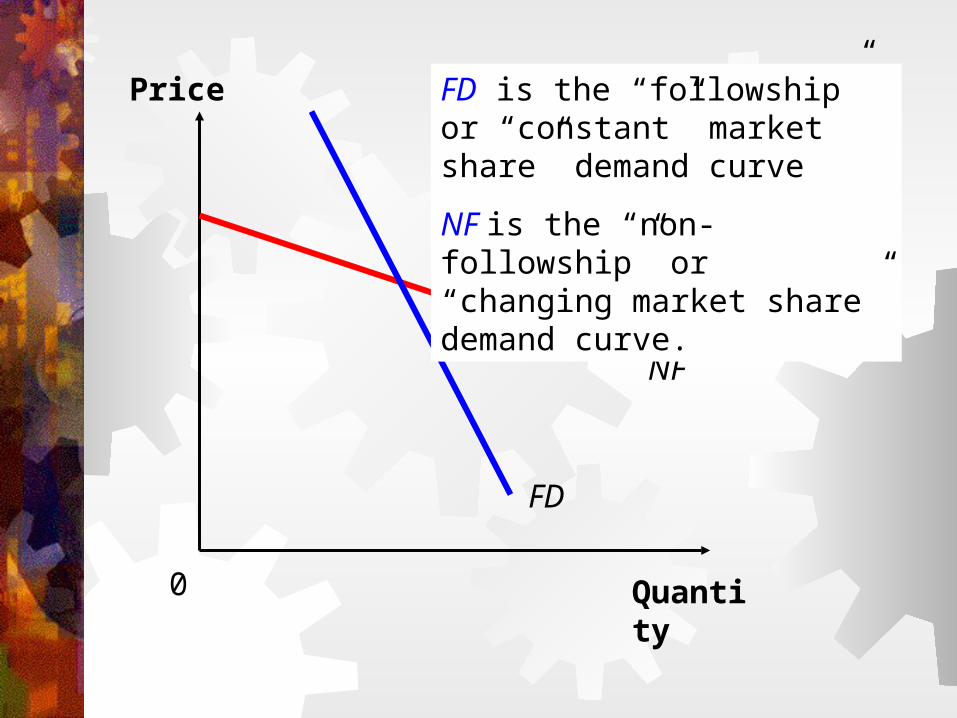
Price

Quantity0

NF

FD

FD is the “followship” or “constant” market share” demand curve

NF is the “non-followship” or “changing market share” demand curve.

If the firm assumes that rivals will ignore (that is, fail to match) price

cuts or increases, then NF is relevant. However, if the firm

assumes that rivals will follow any price adjustments, then FD

applies.

Which demand curve is relevant?

It is reasonable to assume that rivals will

follow price cuts,but not price increases. In that case, the firm faces a

“kinked” demand curve

0

Price

Quantity

FD

NF

KP0

q0

Firm faces NF above the kink and FD below the kink.

0

Price

Quantity

KP0

q0

Incentive to Price At the Kink

> 1

< 1

•Above P0, demand is elastic—hence by raising price revenue will decrease.

•Below P0, demand is elastic—hence by decreasing price revenue will decrease.

Marginal cost can vary in a wide range and the results do not change

P*Demand

MCMC'

MR

Q*

Dollars per Unit of Output

Output