HAL Id: tel-03264167https://tel.archives-ouvertes.fr/tel-03264167

Submitted on 18 Jun 2021

HAL is a multi-disciplinary open accessarchive for the deposit and dissemination of sci-entific research documents, whether they are pub-lished or not. The documents may come fromteaching and research institutions in France orabroad, or from public or private research centers.

L’archive ouverte pluridisciplinaire HAL, estdestinée au dépôt et à la diffusion de documentsscientifiques de niveau recherche, publiés ou non,émanant des établissements d’enseignement et derecherche français ou étrangers, des laboratoirespublics ou privés.

On automata networks dynamics : an approach based oncomputational complexity theory

Martín Ríos Wilson

To cite this version:Martín Ríos Wilson. On automata networks dynamics : an approach based on computational com-plexity theory. Dynamical Systems [math.DS]. Aix-Marseille Université et LIS- CANA, 2021. English.�tel-03264167�

THÈSE DE DOCTORATSoutenue à la Universidad de Chile, Santiago, Chilidans le cadre d’une cotutelle avec la Universidad de Chilele 31 mai 2021 par

Martín Ríos WilsonOn automata networks dynamics : an approach based on

computational complexity theory

DisciplineInformatique

École doctoraleED 184 Mathématiques et informatique

LaboratoireLaboratoire d’informatique et systèmes (LIS)

Composition du jury

Enrico Formenti RapporteurProfesseur des universités, Univ. Côte d’Azur

Eric Goles Co-encadrantProfesseur des universités, Univ. Adolfo Ibañez

Jarkko Kari RapporteurProfesseur des universités, Univ. Turku

Alejandro Maass Co-directeurProfesseur des universités, Univ. Chile

Ivan Rapaport ExaminateurProfesseur des universités, Univ. Chile

Sylvain Sené Co-directeurProfesseur des universités, Univ. Aix-Marseille

Véronique Terrier ExaminatriceMaître de conférences, Univ. Caen

Guillaume Theyssier Co-encadrantChargé de recherche, CNRS (Marseille)

UNIVERSIDAD DE CHILEFACULTAD DE CIENCIAS FÍSICAS Y MATEMÁTICASDEPARTAMENTO DE INGENIERÍA MATEMÁTICA

ON AUTOMATA NETWORKS DYNAMICS: AN APPROACH BASED ONCOMPUTATIONAL COMPLEXITY THEORY

TESIS PARA OPTAR AL GRADO DEDOCTOR EN CIENCIAS DE LA INGENIERÍA, MENCIÓN MODELACIÓN

MATEMÁTICAEN COTUTELA CON AIX-MARSEILLE UNIVERSITÉ

MARTÍN ALONSO FACUNDO RÍOS WILSON

PROFESORES GUÍA:ALEJANDRO MAASS SEPÚLVEDA

SYLVAIN SENÉ

PROFESORES CO-GUÍA:ERIC GOLES CHACC

GUILLAUME THEYSSIER

MIEMBROS DE LA COMISIÓN:ENRICO FORMENTI

JARKKO KARIIVAN RAPAPORT ZIMERMANN

VÉRONIQUE TERRIER

Este trabajo ha sido parcialmente financiado por ANID-BECA DOCTORADONACIONAL 2018- FOLIO N° 21180910, CMM ANID PIA AFB170001 and ANR project

ANR-18-CE40-0002

SANTIAGO DE CHILE2021

I, undersigned, Martín Ríos Wilson, hereby declare that the work presented in thismanuscript is my own work, carried out under the scientific direction of AlejandroMaass and Sylvain Sené, and the co-supervision of Eric Goles and Guillaume Theyssier,in accordance with the principles of honesty, integrity and responsibility inherent tothe research mission. The research work and the writing of this manuscript have beencarried out in compliance with both the french national charter for Research Integrityand the Aix-Marseille University charter on the fight against plagiarism.

According to the cotutelle agreement, this work has also been submitted to theUniversidad de Chile, but has not been submitted previously either in this countryor in another country in the same or in a similar version to any other examination body.

Santiago, Chile, the 2nd of April 2021.

This work is made available under the terms of the Creative Commons Licence –Attribution –NonCommercial – NoDerivatives 4.0 International.

Résumé

Un réseau d’automates (RA) est un réseau d’entités (les automates) en interaction.Ces automates ont un nombre fini d’états possibles et sont reliés les uns aux autres parune structure de graphe appelée graphe d’interaction. Chaque automate évolue aucours du temps discret en fonction des états de ses voisins dans le graphe d’interaction,ce qui définit un système dynamique. Ce travail de thèse explore deux questionsprincipales : a) quel est le lien entre les propriétés dynamiques et calculatoires d’unRA? et b) quel est l’impact de la topologie du graphe d’interaction sur la dynamiqueglobale d’un RA?.

Pour aborder la première question, une notion de complexité calculatoire est définieau regard de problèmes de décision liés à la dynamique des RA. De même, une notionde complexité dynamique est définie en termes de l’existence d’attracteurs de périodeexponentielle. Un lien fort entre ces deux définitions est présenté qui met en exerguele concept de simulation entre familles de RA. Dans ce contexte, la complexité secaractérise d’un point de vue localisé en étudiant l’existence de structures appeléesgadgets qui satisfont deux propriétés : i) ils peuvent interagir localement de manièrecohérente comme des systèmes dynamiques et ii) ils sont capables de simuler unensemble fini de fonctions définies sur un ensemble fini.

La deuxième question est quant à elle abordée dans le contexte des RA “freezing”. UnRA est “freezing” s’il y a un ordre sur les états de telle sorte que l’évolution de l’état den’importe quel automate ne diminue pas quelle que soit l’orbite. Un problème généralde model-checking capturant de nombreux problèmes de décision classiques estprésenté. De plus, lorsque trois paramètres de graphe, le degré maximum, la largeurarborescente et la taille de l’alphabet sont bornés, un algorithme parallèle efficacerésolvant le problème mentionné est donné. De plus, il est montré que ce problèmeest peu susceptible d’être FPT (fixed-parameter tractable) lorsque le paramètre delargeur arborescente ou celui de taille de l’alphabet sont considérés comme uniqueparamètre.

Abstract

An automata network (AN) is a network of entities, each holding a state from a finiteset and related by a graph structure called an interaction graph. Each node evolvesaccording to the states of its neighbors in the interaction graph, defining a discretedynamical system. This thesis work explores two main questions : a) what is the linkbetween dynamical and computational properties of an AN ? and b) what is the impactof the interaction graph topology on the global dynamics of an AN ?.

In order to tackle the first question a notion of computational complexity of anAN family is defined in terms of the computational complexity of decision problemsrelated to the dynamics of the network. On the other hand, dynamical complexity of aparticular AN family is defined in terms of the existence of attractors of exponentialperiod. A strong link between these two last definitions is presented in terms of thenotion of simulation between AN families. In this context, complexity is characterizedfrom a localized standpoint by studying the existence of structures called coherentgadgets which satisfy two properties : i) they can locally interact in a coherent wayas dynamical systems and ii) they are capable of simulating a finite set of functionsdefined over a fixed finite set.

Finally, the second question is addressed in the context of a well-known familycalled freezing automata networks. An AN is freezing if there is an order on statessuch that the state evolution of any node is non-decreasing in any orbit. A generalmodel checking problem capturing many classical decision problems is presented.In addition, when three graph parameters, the maximum degree, the treewidth andthe alphabet size are bounded, a fast-parallel algorithm that solves general modelchecking problem is presented. Moreover, it is shown that the latter problem is unlikelyto be fixed-parameter tractable on the treewidth parameter as well as on the alphabetsize when considered as single parameters.

Publications

The present work is based in the following articles:

• Journals

– 2021. On the Complexity of Asynchronous Freezing Cellular Automata, EricGoles, Diego Maldonado, Pedro Montealegre, Martín Ríos Wilson, Informationand Computation,104764, ISSN 0890-5401.

– 2021. Generating Boolean functions on totalistic automata networks, AndrewAdamatzky, Eric Goles, Pedro Montealegre, Martín Ríos Wilson, InternationalJournal of Unconventional Computing, (to appear).

– 2020. On the effects of firing memory in the dynamics of conjunctive networks,Eric Goles, Pedro Montealegre, Martín Ríos Wilson, Discrete and ContinuousDynamical Systems - A, 40(10): 5765-5793.

• Preprints

– 2021. On Symmetry versus Asynchronism: at the Edge of Universality in Au-tomata Networks, Martín Ríos Wilson, Guillaume Theyssier, arXiv:2105.08356.https://arxiv.org/abs/2105.08356

– 2020. On the impact of treewidth in the computational complexity of freezing dy-namics, Eric Goles, Pedro Montealegre, Martín Ríos Wilson, Guillaume Theyssier,arXiv:2005.11758. https://arxiv.org/abs/2005.11758

• Conferences

– 2021. On the impact of treewidth in the computational complexity of freezing dy-namics, Eric Goles, Pedro Montealegre, Martín Ríos Wilson, Guillaume Theyssier,Computability in Europe 2021: Connecting with Computability. Accepted.

– 2019. On the effects of firing memory in the dynamics of conjunctive networks,Eric Goles, Pedro Montealegre, Martín Ríos Wilson, International Workshop onCellular Automata and Discrete Complex Systems (pp. 1-19). Springer, Cham.

• Book chapters

– 2021. Computing the Probability of Getting Infected: On the Counting Com-plexity of Bootstrap Percolation, Pedro Montealegre and Martín Ríos Wilson. In“Automata and Complexity: Essays presented to Eric Goles on the occasion of his70th birthday” (to appear).

ix

Contents

Introduction 1

1 Preliminaries 6

1.1 Automata networks . . . . . . . . . . . . . . . . . . . . . . . . . . . . . . . . 61.1.1 Elements of Graph Theory . . . . . . . . . . . . . . . . . . . . . . . . 61.1.2 Automata networks as discrete dynamical systems . . . . . . . . . . . 81.1.3 Some important automata network families . . . . . . . . . . . . . . . 91.1.4 Bounded degree automata networks . . . . . . . . . . . . . . . . . . . 111.1.5 Algebraic automata networks . . . . . . . . . . . . . . . . . . . . . . 111.1.6 Freezing automata networks . . . . . . . . . . . . . . . . . . . . . . . 111.1.7 Non-deterministic automata networks . . . . . . . . . . . . . . . . . . 12

1.2 Elements of computational complexity . . . . . . . . . . . . . . . . . . . . . 131.2.1 Counting complexity . . . . . . . . . . . . . . . . . . . . . . . . . . . 141.2.2 Parametric complexity . . . . . . . . . . . . . . . . . . . . . . . . . . 161.2.3 Parellel computing and NC . . . . . . . . . . . . . . . . . . . . . . . 17

1.3 Toolbox . . . . . . . . . . . . . . . . . . . . . . . . . . . . . . . . . . . . . . 201.3.1 Automata networks dynamics . . . . . . . . . . . . . . . . . . . . . . 201.3.2 Treewidth and tree decompositions . . . . . . . . . . . . . . . . . . . 211.3.3 Fast parallel subroutines . . . . . . . . . . . . . . . . . . . . . . . . . 211.3.4 Arithmetic results . . . . . . . . . . . . . . . . . . . . . . . . . . . . . 21

2 Measuring dynamical behavior 23

2.1 Automata network representations . . . . . . . . . . . . . . . . . . . . . . . 242.1.1 Representation of some particular families . . . . . . . . . . . . . . . 242.1.2 Computing interaction graphs from representations. . . . . . . . . . . 262.1.3 Standard representation . . . . . . . . . . . . . . . . . . . . . . . . . 27

2.2 Simulation and universality . . . . . . . . . . . . . . . . . . . . . . . . . . . 282.2.1 Simulation between automata networks . . . . . . . . . . . . . . . . . 282.2.2 Simulation between families of automata networks . . . . . . . . . . . 30

2.3 Decision problems and automata network dynamics . . . . . . . . . . . . . . 312.4 Universal automata network families . . . . . . . . . . . . . . . . . . . . . . 34

3 Gadget complexity: from local to global behavior 39

3.1 Putting pieces together: glueing automata networks . . . . . . . . . . . . . . 393.2 Computing on automata networks . . . . . . . . . . . . . . . . . . . . . . . . 42

3.2.1 G-networks . . . . . . . . . . . . . . . . . . . . . . . . . . . . . . . . 42

x

3.2.2 G-gadgets and simulation of G-networks . . . . . . . . . . . . . . . . . 453.2.3 Gadget glueing . . . . . . . . . . . . . . . . . . . . . . . . . . . . . . 46

3.3 Some useful families of G-networks: Gm-networks and Gm,2-networks . . . . . 503.3.1 Closure and synchronous closure . . . . . . . . . . . . . . . . . . . . . 583.3.2 Super-polynomial periods without universality . . . . . . . . . . . . . 593.3.3 Conjunctive networks and Gconj-networks . . . . . . . . . . . . . . . . 603.3.4 Super-polynomial transients without universality . . . . . . . . . . . 62

4 Describing asynchronous dynamics: a deterministic approach 65

4.1 Update schemes . . . . . . . . . . . . . . . . . . . . . . . . . . . . . . . . . . 664.1.1 Periodic update schemes . . . . . . . . . . . . . . . . . . . . . . . . . 664.1.2 Projection systems . . . . . . . . . . . . . . . . . . . . . . . . . . . . 69

5 Concrete symmetric automata networks: a case study 74

5.1 Symmetric conjunctive networks . . . . . . . . . . . . . . . . . . . . . . . . . 755.1.1 Local clocks update scheme . . . . . . . . . . . . . . . . . . . . . . . 755.1.2 Periodic update schemes . . . . . . . . . . . . . . . . . . . . . . . . . 775.1.3 Firing memory schemes . . . . . . . . . . . . . . . . . . . . . . . . . . 80

5.2 Locally positive symmetric signed conjunctive networks . . . . . . . . . . . . 895.2.1 Block sequential update schemes . . . . . . . . . . . . . . . . . . . . 895.2.2 Local clocks update schemes . . . . . . . . . . . . . . . . . . . . . . . 89

5.3 Symmetric signed conjunctive networks . . . . . . . . . . . . . . . . . . . . . 905.3.1 Block sequential update schemes . . . . . . . . . . . . . . . . . . . . 91

5.4 Symmetric min-max networks . . . . . . . . . . . . . . . . . . . . . . . . . . 1025.4.1 Block sequential update schemes . . . . . . . . . . . . . . . . . . . . 103

6 Freezing dynamics 106

6.1 Specification checking problem: a canonical model checking problem to cap-ture many classical dynamical problems. . . . . . . . . . . . . . . . . . . . . 1076.1.1 Localized Trace Properties . . . . . . . . . . . . . . . . . . . . . . . . 1086.1.2 A fast parallel algorithm for Specification Checking . . . . . . . . . . 1136.1.3 W[2]-hardness results . . . . . . . . . . . . . . . . . . . . . . . . . . . 1216.1.4 Hardness results for polynomial treewidth networks . . . . . . . . . . 124

6.2 Counting complexity on freezing automata networks: a case study. . . . . . . 1326.2.1 Contagion-Probability is #P -Complete . . . . . . . . . . . . . . 1356.2.2 Polynomial time algorithm for maximum degree 4 . . . . . . . . . . . 142

Discussion 147

Bibliography 151

xi

List of Tables

5.1 Summary of the main results on complexity of the dynamics of the networkfamilies studied in the current chapter, depending on different update schemes.BPA = Bounded period attractors. SPA = Superpolynomial attractors. SU =Strong universality. Black fonts indicate the emergence of complex behaviorsuch as long period attractors or universality. . . . . . . . . . . . . . . . . . 75

5.2 Dynamics of the central gadgets in an AND gadget implemented over a sym-metric signed conjunctive network. Notation is the same of the one used inFigure 5.17 . . . . . . . . . . . . . . . . . . . . . . . . . . . . . . . . . . . . 97

5.3 Dynamics for central gadgets in OR gadget implemented over a symmetricsigned conjunctive network. Notation is the same of the one shown in Figure5.16 . . . . . . . . . . . . . . . . . . . . . . . . . . . . . . . . . . . . . . . . 101

5.4 Dynamics for context in AND/OR gadgets implemented on symmetric signedconjunctive networks. . . . . . . . . . . . . . . . . . . . . . . . . . . . . . . . 101

xii

List of Figures

2.1 Scheme of one-to-one block simulation. In this case, network F is simulatedby H. Each node in F is assigned to a block in H and state coding is injective.Observe that blocks are connected (one edge in the original graph may be rep-resented by a path in the communication graph of H) according to connectionsbetween nodes in the original network F . This connections are represented byblue lines. . . . . . . . . . . . . . . . . . . . . . . . . . . . . . . . . . . . . . 29

3.1 General scheme of a glueing. . . . . . . . . . . . . . . . . . . . . . . . . . . . 403.2 Symmetry breaking in interaction graph after a glueing operation. Arrows

indicate influence of a node (source) on another (target), edges without arrowindicates bi-directional influence. Here C consists in two nodes only. . . . . . 41

3.3 Example of a glueing of two compatibles CSAN. The labeling in nodes of G1,G2 and G0 shows equalities between local � maps of these three CSAN. . . . 43

3.4 (Left panel) A set of maps G over alphabet Q. (Central panel) An intuitive rep-resentation of input/output connections to make a G-network. (Right panel)The corresponding formal G-network � : Q3 ! Q3 together with the globalmap associated to it. The bijections ↵ and � from Definition 3.4 are repre-sented in blue and red (respectively). . . . . . . . . . . . . . . . . . . . . . . 44

3.5 Gadget glueing as in Definition 3.6. (Left panel) Two gadgets with interfaceC = Ci [ Co where Ci part in each copy of the interface dowel is in red andCo part in blue. The gadget glueing is done with input �F (A) on output�G(A) (here A is a singleton) and output ⌧F (B) on input ⌧G(B) (B is also asingleton). (Top right panel) A representation of the global glueing processwhere nodes in green are those in the copy of CF in F or in the copy CG in G;dotted links show the bijection between the embeddings of C = CF [ CG intoVF and VG via maps �F and �G. (Bottom right panel) The resulting gadgetwith the same interface C = Ci [ Co as the two initial gadgets. . . . . . . . . 47

3.6 AND and OR gadgets for simulating AND/OR gates with fanin and fanout2. For other values of fanin and fanout gadgets are the same but consideringdifferent number of inputs/outputs. . . . . . . . . . . . . . . . . . . . . . . . 52

3.7 NOT gadget wiring for circuit simulation using gates from Gm. In this case aNOT gate is connected to an OR gate in the original circuit. Copies of theNOT gate in the circuit performing simulation are connected to the copies ofthe OR gate switched: positive part is connected to negative part of the ORgate and viceversa. . . . . . . . . . . . . . . . . . . . . . . . . . . . . . . . . 52

xiii

3.8 Block gadgets for simulating fanin 2 fanout 1 AND/OR gates using only gatesin Gm,2. Squared zeros represent the amount of zeros that can be used asinputs for the same block. Circled zeros correspond to extra zeros that needto be received from a Fanin 1 Fanout 2 gate. . . . . . . . . . . . . . . . . . . 55

3.9 Block gadgets for simulating fanin 1 fanout 2 and fanin 1 fanout 1 AND/ORgates using only gates in Gm,2. Squared zeros represent the amount of zerosthat can be used as inputs for the same block. Circled zeros correspond toextra zeros that need to be received from a fanin 2 fanout 1 gate. . . . . . . 56

3.10 Block gadgets for simulating fanin 2 fanout 2 AND/OR gates using only gatesin Gm,2. Squared zeros represent the amount of zeros that can be used asinputs for the same block. . . . . . . . . . . . . . . . . . . . . . . . . . . . . 57

3.11 (Left panel) Non-synchronous composition and (Right panel) synchronouscomposition. . . . . . . . . . . . . . . . . . . . . . . . . . . . . . . . . . . . . 59

3.12 Fanin gadget of degree 3. For any configuration x, F 3(x)vo = xv1 ^ xv2 ^ xv3 . 61

3.13 Freezing the result of a test in a Gt-network. The module T (x) is made ofthe nodes marked ⌥, AND2, ⇤ and Id. Observe that each node representsome output of its corresponding label(for more details on G-networks seeDefinition 3.4). Each gate has one output with the exception of the gate ⌥

which is represented by two nodes. The module T (x) reads the value of nodex belonging to an arbitrary Gt-network (represented in light gray inside dottedlines). The output ⇤ is fed back to its control input via the Id node (self-loopsare forbidden in Gt-networks). Note that x as well as the rest of the networkis not influenced by the behavior of the gates of the module T (x). . . . . . . 63

4.1 Synchronous update scheme and sequential update scheme for the same con-junctive automata network. (Left panel) communication graph of the network.Local function is given by the minimum (AND function) over the set of statesof neighbors for each node. (Central panel) Synchronous or parallel updatescheme and the associated dynamics of configuration (0, 1, 1, 0). In this case µhas period 1 and all nodes are updates simultaneously. Observe that dynamicsexhibits an attractor of period 2 (Right panel) Sequential update scheme andthe associated dynamics of configuration (0, 1, 1, 0). In this case function µhas period n = 4 and only one node is updated at each time step. Dynamicsreach a fixed point given by ~0. . . . . . . . . . . . . . . . . . . . . . . . . . . 67

4.2 A block sequential and a local clocks update schemes over a simple conjunctivenetwork. (Left panel) communication graph of the network. Local functionsare given by the minimum (AND) over the states of the neighbors of each node.(Central panel) block sequential update scheme and the associated dynamics ofconfiguration (0, 1, 1, 0). In this case function µ is defined by two blocks: {1, 3}and {2, 4}. Dynamics reach a fixed point after 3 time steps. (Right panel) localclocks update scheme and the associated dynamics of configuration (0, 1, 1, 0).In this case each node has an internal clock with different local periods. Nodes1 and 3 are updated every two steps (p1 = p3 = 2) and nodes 2 and 4 areupdated every 4 time steps (i.e. p2 = p4 = 4). The shift parameters is 0 forall nodes ⌧1 = ⌧2 = ⌧3 = ⌧4 = 0. The dynamics reaches a fixed point after 5

time steps. . . . . . . . . . . . . . . . . . . . . . . . . . . . . . . . . . . . . . 68

xiv

4.3 A general periodic update scheme over a conjunctive network. In this caseµ has period 4 and the underlying dynamics reaches a fixed point after 4

time steps. Observe that there is no restriction on how many times a nodeis updated. For example, 1 is updated 3 times every 4 time steps but 4 isupdated only twice every 4 time steps. . . . . . . . . . . . . . . . . . . . . . 68

4.4 A block parallel update scheme defined over a conjunctive network. Updatinglist is given by L = {(1), (2, 3), (4)}. Observe that a constant amount of nodes(equal to the length of L, i.e., 3) is updated at each time step. Dynamicsreaches a fixed point after 3 time-steps. . . . . . . . . . . . . . . . . . . . . . 69

4.5 A firing memory update scheme over a conjunctive network. Each local func-tion is given by the minimum over the states of neighbors. The delay compo-nent (second component in Definition 4.8) only is shown. Maximum delay ofthe network is ⌧ = 4. Dynamics describes an attractor of period 4 in which0 circulates over the different nodes of the network. Note that at any time,there is exactly one node in state 0, the other being in state 1 with differentdelay values. . . . . . . . . . . . . . . . . . . . . . . . . . . . . . . . . . . . . 73

5.1 Scheme of the dynamics of nodes i, k and ` defined in the proof of Lemma5.1. The checkmarks indicate where it is feasible for ` to be updated and thecrosses mark the intervals on which ` can change its state. . . . . . . . . . . 77

5.2 Clock gadget implemented in a conjunctive network with firing memory. (Leftpanel) The interaction graph of the clock gadget. (Right panel) The dynamicsof an attractor of period 3. . . . . . . . . . . . . . . . . . . . . . . . . . . . . 81

5.3 The glueing interface considered for AND/OR gadgets implemented over aconjunctive network with firing memory. The labels given by marking func-tions ' are assigned in each gadget accordingly. . . . . . . . . . . . . . . . . 83

5.4 The initial condition and structure for AND/OR gadgets implemented overconjunctive networks with firing memory. (Upper panel) the AND gadget.(Bottom panel) the OR gadget. The variables (x, y) 2 {0, 1}2 represent thebits that the gadget is considering as inputs and z 2 {0, 1} is a bit that isgoing to serve as an input for other gadget. Total computation takes T = 9

time steps. The triangles represent clock gadgets. The dashed boxes mark theembedded copies of the glueing interface which plays the role of output/input. 83

5.5 The first three steps of the dynamics of the AND gadget implemented ina conjunctive network with firing memory. The variables (x, y) 2 {0, 1}2represent the bits that the gadget is considering as inputs and z 2 {0, 1} isa bit that is going to serve as an input for other gadget. Total computationtakes T = 9 time steps. The triangles represent clock gadgets. The dashedboxes mark the embedded copies of the glueing interface which plays the roleof output/input. . . . . . . . . . . . . . . . . . . . . . . . . . . . . . . . . . . 84

5.6 The fourth to sixth steps of the dynamics of the AND gadget implementedin a conjunctive network with firing memory. The variables (x, y) 2 {0, 1}2represent the bits that the gadget is considering as inputs. Total computationtakes T = 9 time steps. The triangles represent clock gadgets. The dashedboxes mark the embedded copies of the glueing interface which plays the roleof output/input. . . . . . . . . . . . . . . . . . . . . . . . . . . . . . . . . . . 85

xv

5.7 The final four steps of the dynamics of the AND gadget implemented in a con-junctive network with firing memory. The variables (x, y) 2 {0, 1}2 representthe bits that the gadget is considering as inputs. The variables (x0, y0) 2 {0, 1}2represent the new information that the gadget is receiving as inputs. Totalcomputation takes T = 9 time steps. The triangles represent clock gadgets.The dashed boxes mark the embedded copies of the glueing interface whichplays the role of output/input. . . . . . . . . . . . . . . . . . . . . . . . . . . 86

5.8 The first five steps of the OR gadget implemented in a conjunctive networkwith firing memory. The variables (x, y) represent the bits that the gadget isconsidering as inputs and z 2 {0, 1} correspond to some bit that is going tobe send as input of other gadget. The function k(x, y) is defined by k(0, 0) =0, k(1, 0) = k(1, 1) = 2 and k(0, 1) = 1. Total computation takes T = 9 timesteps. Triangles represent clock gadgets and different states are part of thecontext configurations. The dashed boxes mark the embedded copies of theglueing interface C which plays the role of outputs/inputs. . . . . . . . . . . 87

5.9 The last four steps of the OR gadget implemented in a conjunctive networkwith firing memory. The variables (x, y) represent the bits that the gadgetis considering as inputs and (x0, y0) 2 {0, 1}2 correspond to new informationthat the gadget is interpreting as inputs. Total computation takes T = 9 timesteps. Triangles represent clock gadgets and different states are part of thecontext configurations. The dashed boxes mark the embedded copies of theglueing interface C which plays the role of outputs/inputs. . . . . . . . . . . 88

5.10 One step of the dynamics of the NOT part of AND/OR gadget implemented bya symmetric signed conjunctive network. Dashed ellipses and parallelogramsrepresent blocks. Each block is labeled by its corresponding number (1, 2 and3) in a gray colored circle. Thick dashed rectangle highlights nodes in thecentral part. All edges are negative. Each time step t is taken after three timesteps (one for each block). Total simulation time is T = 9. . . . . . . . . . . 92

5.11 Two last steps of the dynamics described by the NOT part of AND/OR gadgetsimplemented by a symmetric signed conjunctive network. Dashed ellipses andparallelograms represent blocks. Each block is labeled by its correspondingnumber (1, 2 and 3) in a gray colored circle. Thick dashed rectangle highlightsnodes in the central part. All edges are negative. Each time step t is takenafter three time steps (one for each block). Total simulation time is T = 9. . 93

5.12 Wire gadget implemented on a signed symmetric conjuntive network. 2 copiesof NOT gadget are combined in order to form a wire. Simulation time isT = 6⇥ 3. . . . . . . . . . . . . . . . . . . . . . . . . . . . . . . . . . . . . . 94

5.13 Scheme of labeling for 4-cycles in AND/OR gadgets. Notation is given by thefollowing guidelines: s represent the associated group of three nodes, secondtwo coordinates indicate its position relative the group of three nodes and itsposition in the 4-cycle graph (considering counter clock-wise order), and u, lstands for upper or lower according to its position in the gadget. . . . . . . . 97

xvi

5.14 One step of the dynamics of the computation gadget inside AND/OR gadgetimplemented by a symmetric signed conjunctive network. Dashed ellipses andparallelograms represent blocks. Each block is labeled by its correspondingnumber (1, 2 and 3) in a gray colored circle. Thick dashed rectangle highlightsnodes in the central part. All edges are negative. Each time step t is takenafter three time steps (one for each block). Total simulation time is T = 9. . 98

5.15 Last two steps of the dynamics of the computation gadget inside AND/ORgadget implemented by a symmetric signed conjunctive network. Dashed el-lipses and parallelograms represent blocks. Each block is labeled by its corre-sponding number (1, 2 and 3) in a gray colored circle. Thick dashed rectanglehighlights nodes in the central part. All edges are negative. Each time step tis taken after three time steps (one for each block). Total simulation time isT = 9. . . . . . . . . . . . . . . . . . . . . . . . . . . . . . . . . . . . . . . . 99

5.16 OR gadget structure. In order to produce a OR gadget, wire gadget and NOTgadget are combined with the computation part depicted in Figures 5.14 and5.15. . . . . . . . . . . . . . . . . . . . . . . . . . . . . . . . . . . . . . . . . 100

5.17 AND gadget structure. In order to implement an AND gadget, wire gadgetand NOT gadget are combined with the computation part depicted in Figures5.14 and 5.15. . . . . . . . . . . . . . . . . . . . . . . . . . . . . . . . . . . . 100

5.18 Gadget used for simulation of a symmetric signed conjunctive network witharbitrary periodic update scheme implemented over an AND-OR network withperiodic update scheme. . . . . . . . . . . . . . . . . . . . . . . . . . . . . . 105

6.1 Checking that the same node is marked in each bloc in a selection row: onthe left, a valid test in bloc p, on the right an invalid test in bloc p generatingan error state. Dotted lines indicate the marked position in each bloc. Theshades of gray indicates the state changes involved in the implementation offreezing signals: at each position the sequence of states in non-decreasing withtime. . . . . . . . . . . . . . . . . . . . . . . . . . . . . . . . . . . . . . . . . 123

6.2 Gadgets used to construct graph G[F , k]. (Left upper panel) variable gad-get. (Right upper panel) clause gadget. (Left bottom panel) threshold gad-get.(Right bottom panel) output gadget. Gray nodes are active and whitenodes are inactive. . . . . . . . . . . . . . . . . . . . . . . . . . . . . . . . . 137

6.3 Scheme representing graph G[F , k]. Each type of gadget is detailed in Figure6.2. . . . . . . . . . . . . . . . . . . . . . . . . . . . . . . . . . . . . . . . . . 139

xvii

xviii

Introduction

An automata network is a collection of n entities, called automata (and sometimes also re-ferred as nodes or vertices), which are somehow related. These relations between the differententities are represented by a graph structure and are defined in this document by local func-tions which take values in a finite set, usually denoted by Q and called the alphabet. From aglobal standpoint, these local functions can be seen as a global function acting on set Qn anddefining a dynamical system (which can be deterministic or not deterministic). The mostcommon and natural way to define the dynamics of an automata network is just consideringdeterministic local rules for each node in the network. However, it is also interesting to con-sider the non-deterministic case, which also includes probabilistic and asynchronous models.In particular, a way to introduce asynchronism consists in updating only some of the nodesin the network at a time step and leave the state of the others unchanged. Then, for eachtime step, there exists an assignation of nodes that will update their states at this step. Suchassignations define an update scheme.

Observe that, the automata network model can be considered as a topological non-uniformgeneralization of (finite) cellular automata. Automata networks have been used as modellingtools in many areas [36] and they can also be considered as a distributed computationalmodel with various specialized definitions like in [79, 80].

Generally speaking, two main research lines can be identified in the context of the studyof this model. The first one is related to the dynamics that an automata network can haveaccording to the updating modes. It focuses particularly on analyzing their richness in termsof, for instance, the period of attractors compared to the size of the network and, in this sense,the role that graph topology plays in restricting or allowing complex dynamical behavior. Thesecond one is more focused on the computation abilities of the network. In this approach,decision problems related to the dynamics of the network are proposed. A very interestingone, that we study in this thesis, is called the prediction problem. Roughly speaking, onewould want to see if it is possible to predict the dynamical behavior of the network. Moreprecisely, a particular node in the network is fixed and an initial configuration is given forthe rest of the nodes in the network. We would like to know if at some given time step t (ormaybe if eventually) the state of this node will change or if it will remain as in the initialconfiguration. Of course, there is always a trivial solution to this problem, which consists insimply simulating the network for t time steps (or if there is no given time limit, we simulateuntil reaching an attractor) and see if our objective node has changed. Thus, a naturalquestion in this context is if we can beat simulation in someway by finding an algorithm thatis more efficient than simply simulating. Generally speaking, if the dynamics is extremely

1

difficult to predict (there is no way of beating simulation) the system is complex. Contrarily,if there exists some particular algebraic or graph topology property which we can exploit todesign an algorithm to decide prediction problem in an efficient way (compared to the trivialsolution) then, the system is not complex. Within this framework, an interesting observationconcerning local dynamical behavior arises. Observe that there are some similarities betweenprediction problem and, in the context of Boolean circuit families, the well-known circuitvalue problem. This problem consists in, given a Boolean circuit and an assignation of itsinputs, evaluating the circuit and read some fixed output value. In this sense, in many studycases we would like to show that there exists a suitable reduction from this problem to theprediction problem. In fact, given some class of automata networks (which can be defined bya particular type of rule) this task is somehow translated to the task of simulating in somecoherent way the gates of the circuit. This is achieved by using some particular collectionof subnetworks in the class that implements (understanding this as some sort of simulationimplemented using its dynamics) each different type of gate in the circuit and which can beglued together in a coherent way so that the resulting glued module simulates the circuitevaluation process.

The main aim of this thesis is twofold: on the one hand to provide a general theoreti-cal framework which would allow to unify both research lines by exhibiting a link betweencomputational capabilities of an automata network and its dynamical behavior; on the otherhand to study how the graph structure of a network can impact the dynamics of the latter.In particular, we face this task through two main research questions:

1. What is the link between dynamical and computational properties of an automatanetwork?

2. What is the impact of the interaction graph topology in the global dynamics of anautomata network?

In order to answer these questions, we start by establishing a general framework forautomata networks, including what is precisely a family of automata networks and how torepresent it in a concrete way. We explore a general way to combine different automatanetworks in order to construct a new network preserving dynamical properties from thenetworks used in this combination. This framework allows us to provide sufficient conditionsto deduce global dynamical and computational properties for a particular family by focusingin studying local structures called gadgets. In addition, inspired by the intrinsic simulationframework for cellular automata, we compare the capabilities of different automata networkfamilies by developing a definition for simulation between families. More precisely, we developa simulation scheme based on an injective assignment of states in the simulated network toa subgraph in the simulator. We call these subgraphs blocks and we represent each nodethe simulated network by one of this subgraphs in the simulator. Then, the dynamics of thesimulated network is simulated (possibly several time steps represent a single time transitionon the simulated network dynamics) by this latter injective coding in each block. This latterdefinition of simulation, does not only allow us to transfer dynamical properties from thesimulated network to the simulator but also help us to deduce computational complexityresults regarding the prediction problem in the simulator by studying the simulated network.This is possible because our definition of simulation is compatible with standard polynomialand logspace reductions. We go further in this context by stating the concept of universality

2

for automata networks, expressed as the capability to efficiently simulate families of automatanetworks. These families can be described by a family of circuits, each one representing anautomata network in this family. We ask these circuit families to satisfy that the maximumnumber of gates in a circuit grows bounded by a polynomial function on the size of therepresented network. In particular, we study the case of automata networks in which its graphhas a maximum degree bounded by a constant (not depending on the size of the network)and we propose a stronger definition of universality related to the capability of simulatingthis latter family. We then, apply our framework to a concrete case of study, composed bydifferent families of automata networks and different update schemes. Roughly, we considera pool of automata network families sharing a common set of properties and we establish apartial hierarchy in the set of families given by different constraints. In parallel, we have alsoa hierarchy in update schemes. We observe an interesting trade-off between the constraintswe can apply in a particular family and the constraints we can apply related to the updatescheme we are considering. Particularly, we observe that families with more constraintsequipped with general update schemes are universal, but they can lose this property if weapply constraints in the type of update scheme we are considering and complementarily, if westart with more general families, we can observe universality when family is equipped withmore restricted update schemes.

Then, we tackle the second question by considering a particular family of automata net-work, called freezing automata networks. An automata network is freezing if there is an orderon states such that the state evolution of any node is non-decreasing in any orbit. In this partof the thesis, we go beyond the deterministic definition of automata networks and we studythe non-deterministic case in the context of freezing networks. We define in this context ageneralization of the prediction problem called the specification problem which also includessome other decision problems related to the dynamics of an automata network. Then, we ex-plore the impact of the graph topology on the dynamics by identifying key graph parameterswhich allow us to design efficient algorithms for solving the latter problem. We address thislatter challenge from a parametric complexity approach. Finally, we study the particularversion of bootstrap percolation model, consisting in a freezing version of the well-knownmajority automata. In this latter network, each node takes the state of the majority of itsneighbors in the graph. We see this model as a disease spreading model and we study thecomplexity of the functional problem consisting in computing the probability of some node toget infected. We then establish that in general the problem is hard since a polynomial timealgorithm to compute probability is unlikely to exist. Then, we give sufficient conditions onthe graph in order to assure that probability can be computed in polynomial time.

Related work

There is a wide amount of literature for the prediction problem at sake in this thesis work[46, 61, 37, 34, 39, 38] in which the computational complexity of the latter problem have beenstudied for cellular automata and different automata network families such as: the freezingversion of the well-known game of life called, Life without death, and threshold networksamong which are majority networks and conjunctive networks.

Moreover, the notion of intrinsic universality in cellular automata have been addressedin several papers [49, 8, 60, 64, 65] and it is based on the concept of sub-automaton which

3

consists in a restriction on the set of states and the concept of rescaling which consists inpacking cells. Roughly speaking, a cellular automaton simulates another one if some rescalingof the first one contains a rescaling of the second one as a sub-automaton. In this sense, acellular automaton is intrinsically universal if for any arbitrary other automaton there existssome rescaling of the first which contains it as a sub-automaton.

Regarding freezing automata networks, several models that received a lot of attentionin the literature are actually freezing automata networks, for instance: bootstrap percola-tion which has been studied on various graphs [1, 6, 5, 48], epidemic [25] or forest fire [4]propagation models 1, cristal growth models [75, 43] and more recently self-assembly tilings[78]. Moreover, their complexity as computational models has been studied from variousstandpoints: as language recognizers where they correspond to bounded change or boundedcommunication models [77, 56, 13], for their computational universality [66, 31, 9], as wellas for various associated decision problems [33, 35, 41, 34].

A major topic of interest in automata networks theory is to determine how the networkgraph affects dynamical or computational properties [26, 41]. In the freezing case, it wasfor instance established that one-dimensional freezing cellular automata, while being Turinguniversal via Minsky machine simulation, have striking computational limitations when com-pared to bi-dimensional ones: they are NL-predictable (instead of P-complete) [66, 46, 77],can only produce computable limit fixed points starting from computable initial configura-tions (instead of non-computable ones starting from finite configurations) [66], and have apolynomial time decidable nilpotency problem (instead of uncomputable) [66].

Regarding specifically the complexity of the dynamics of bootstrap percolation, we presentthe following related work: in [41] it is studied the Stability problem which is the decisionproblem consisting in deciding, given a graph and an initial condition, whether an objectivenode reaches state 1 in some time-step, when the states evolve according to the synchronousbootstrap percolation dynamics. This problem is solvable in polynomial time, since thedynamics reaches a fixed point in a linear number of synchronous time-steps. Interestingly,in [41] is shown that in graphs of degree at most 4 the problem is in class NC, which is thesubclass of P containing all problems that can be efficiently solved by a parallel machine.Moreover, in graphs of maximum degree at least 5 the Stability problem is P-Complete,meaning that there is no algorithm solving the problem better than simply simulating thedynamics until a fixed point is reached.

Later, as we mentioned before, in [38] the authors study the complexity of bootstrappercolation on asynchronous updating schemes. To do so, two decision problems are defined.The first one is Good-Sequence (which is called asynchronous prediction in [38]).The second one is called Asyncronous Stability, and is an asynchronous version of thestability problem. The difference between the two problems is that Good-Sequence asksfor the existence of a good-sequence for a given time-span, while Asynchronous Stabilityasks for the state of the node once the attractor is reached. In that article, it is shown thatgiven an initial condition, the dynamics of bootstrap percolation reaches the same fixed pointfor every updating scheme. That makes Asyncronous Stability equivalent to Stability.

1They are discrete counterparts of the family of spatial SIR/SEIR models [53] (or other variants) whichare sadly famous amid the actual COVID-19 pandemic.

4

Contrarily, problem Good-Sequence is solvable in polynomial time when restricted tographs maximum degree 4, but NP-Complete restricted to graphs of maximum degree 5.

Chapter structureThis thesis work is divided in six chapters. The first chapter contains basic definitions andresults that are used to derive main results of this work. This includes some elements ofcomputational complexity and graph theory and some related results in the dynamics ofautomata networks as well as the definition of some particular families of automata networksthat we will study.

The second chapter develops the main framework on computational complexity and de-cision problems related to automata networks. It starts with a precise definition on therepresentation of different automata network families. Then, it continues with the devel-opment of a general simulation background. This chapter goes beyond this latter point byexploring the notion of universality in the context of the latter definition.

The third chapter presents the framework about gadgets and how the existence of localstructures has an impact on the global dynamics of automata networks. In first place, a familyof bounded degree automata networks, G-networks, is presented. Then, the notion of gadgetis introduced and a scheme for glueing automata networks is developed. Finally, some usefulG-networks are introduced and studied in order to illustrate the relation between universalityand the richness of the dynamics of some families in terms of periods and transients.

The fourth chapter gives a framework about update schemes. First, basic definitions onupdate schemes are provided. Then, the notion of projection system and asynchronous exten-sion is introduced as a way to obtain a general formalism to study asynchronous dynamics.

The fifth chapter is a case of study in which the dynamics of different families of automatanetworks is studied under different update schemes. First, some of the main results are statedand then chapter is divided in sections, each one devoted to the study of one particular family.Each section is divided in subsections, one of each devoted to the study of the dynamics underone particular update scheme. Then, in each of these sections, the question of whether thatfamily equipped with that specific update scheme is universal is addressed.

Finally, the sixth chapter is devoted to the study of freezing automata networks and it isdivided in two main sections: the first one consists in analyzing the effect of graph topologyon the dynamics of freezing automata networks by studying a generalization of the predictionproblem; the second one is focused on studying a concrete model consisting in the study ofthe complexity of the dynamics of a non-deterministic variant of the bootstrap percolationmodel.

5

Chapter 1

Preliminaries

1.1 Automata networks

In this section, we give the elementary definitions related to automata network theory. Westart by considering some elemental results in graph theory and then, we define the conceptof automata networks and related technical definitions.

1.1.1 Elements of Graph Theory

A graph is a pair G = (V,E) where V and E are finite sets satisfying E ✓ V ⇥ V. Wewill call V the set of nodes and the set E of edges. We call |V | the order of G and weusually identify this quantity by the letter n. Usually, as E and V are finite sets we willimplicitly assume that there exists an ordering of the vertices in V from 1 to n (or from 0

to n� 1). Sometimes we will denote the latter set as [n]. If G = (V,E) and V 0 ✓ V,E 0 ✓ Ewe say that G0 is a subgraph of G. We call a graph P = (V,E) of the form V = {v1, . . . , vn},E = {(v1v2), . . . , (vn�1, vn)} a path graph, or simply a path. We often refer to a path bysimply denoting its sequence of vertices {v1, . . . , vn}. We denote the length of a path byits number of edges and if P = (V,E) with V = {v1, . . . , vn}, we call any vk such that1 < k < n an internal node of P . In addition, if A,B ✓ V are node sets, we say that Pis a A-B path if P = (V,E) is a path such that V = {v1, . . . , vn} and v1 2 A, vn 2 B andno internal node lies in A nor in B. If A = {v} and B = {w} then, we call P a v-w path.Whenever P = (V = {v1, . . . , vn}, E = {(v1v2), . . . , (vn�1, vn)} is a path we call the graph inwhich we add the edge {vn, v1} a cycle graph or simply a cycle and we denote it C whereC = P + {vn, v1}. Analogously, a cycle is denoted usually by a sequence of nodes and itslength is also given by the amount of edges (or vertices) in the cycle. Depending of the lengthof C we call it a k-cycle when k is its length. A non-empty graph is called connected if anypair of two vertices u, v are linked by some path. Given any non-empty graph, a maximalconnected subgraph is called a connected component.

We call directed graph a pair G = (V,E) together with two functions init : E ! V andter : E ! V where each edge e 2 E is said to be directed from init(e) to ter(e) and wewrite e = (u, v) whenever init(e) = u and ter(e) = v. There is also a natural extension

6

of the definition of paths, cycles and connectivity for directed graphs in the obvious way.We say a directed graph is strongly connected if there is a directed path between any twonodes. A strongly connected component of a directed graph G = (V,E) is a maximal stronglyconnected subgraph.

Given a (non-directed) graph G = (V,E) and two vertices u, v we say that u and v areneighbors if (u, v) 2 E. Remark that abusing notations, an edge (u, v) is also denoted byuv. Let v 2 V, we call NG(v) = {u 2 V : uv 2 E} (or simply N(v) when the context isclear) the set of neighbors (or neighborhood) of v and �(G)v = |NG(v)| to the degree of v.Observe that if G0

= (V 0, E 0) is a subgraph of G and v 2 V 0, we can also denote by NG0(v)

the set of its neighbors in G0 and the degree of v in G0 as �(G0)v = |NG0(v)|. In addition, we

define the closed neighborhood of v as the set N [v] = N(v) [ {v} and we use the followingnotation �(G) = max

v2V�v for the maximum degree of G. Additionally, given v 2 V , we will

denote by Ev its set of incident edges, i.e., Ev = {e 2 E : e = uv}. We will use the letter nto denote the order of G, i.e. n = |V |. Also, if G is a graph whose sets of nodes and edgesare not specified, we use the notation V (G) and E(G) for the set of vertices and the set ofedges of G respectively. In the case of a directed graph G = (V,E) we define for a nodev 2 V the set of its in-neighbors by N�

(v) = {u 2 V : (u, v) 2 E} and its out-neighborsas N+

(v) = {u 2 V : (v, u) 2 E}. We have also in this context the indegree of v given by�� = |N�

(v)| and its outdegree given by �+ = |N+(v)|

During the most part of of the this manuscript, and unless explicitly stated otherwise,every graph G will be assumed to be connected and undirected. We define a class or a familyof graphs as a set G = {Gn}n�1 such that Gn = (Vn, En) is a graph of order n.

We say that G is a tree-graph or simply a tree if it does not have cycles as subgraphs.Usually, we distinguish certain node in r 2 V (G) that we call the root of G. Whenever Gis a tree and there is a fixed vertex r 2 V (G) we call G a rooted tree. In addition, we willsay that v 2 V (G) is a leaf if �v = 1. Straightforwardly the choice of r induces a partialorder in the vertices of G given by the distance (length of the unique path) between a nodev 2 V (G) and the root r. We define the height of G (and we write it as h(G)) as the longestpath between a leaf and r. We say that a node v is in the (h(G)� k)-th level of a tree G ifthe distance between v and r is k and we write v 2 Lh(G)�k. We call the children of a nodev 2 Lk all w 2 N(v) such that w is in level k � 1.

Tree decomposition, treewidth and brambles

We now introduce the graph parameter known as treewidth. This parameter indicates how“close” is a graph to a tree graph. In order to introduce this concept, we need first thefollowing definition:

Definition 1.1 Given a graph G = (V,E), a tree decomposition is pair D = (T,⇤) suchthat T is a tree and ⇤ is a family of subsets of nodes ⇤ = {Xt ✓ V | t 2 V (T )} called bagssuch that:

• Every node in G is in some Xt, i.e:S

t2V (T )

Xt = V.

7

• For every e = uv 2 E there exists t 2 V (T ) such that u, v 2 Xt.

• For every u, v 2 V (T ) if w 2 V (T ) is in the v-y path in T , then Xu \Xv ✓ Xw.

We define the width of a tree decomposition D as the amount width(D) = maxt2V (T )

|Xt|� 1.

Given a graph G = (V,E), we define its treewidth as the parameter tw(G) = minD

width(D).In other words, the treewidth is the minimum width of a tree decomposition of G. Note that,if G is a connected graph such that |E(G)| � 2 then, G is a tree if and only if tw(G) = 1.

We now introduce a dual concept related to treewidth, which is called bramble. LetG = (V,E) be a graph and B1, B2 be two subgraphs of G. We say that B1 and B2 touch ifthey share at least a common vertex or if there is some edge e 2 E joining them, i.e. if thereexists e 2 E such that e = (u, v) with u 2 B1 and v 2 B2.

Definition 1.2 Let G = (V,E) a graph. A bramble in G is a set B of connected subgraphsof G such that any B1, B2 2 B touch.

Let G = (V,E) a graph and B a bramble in G. We say that a set of nodes S ✓ V (G) is ahitting set for B if it intersects every subgraph in B. The size of a minimum hitting set forB is known as its order.

Definition 1.3 Let G = (V,E) a graph and let B be a bramble on G. We call B a perfectbramble if:

1. Any two B1, B2 2 B have non-empty intersection.2. For every v 2 V there are at most two subgraphs in B that contains v.

3. Every vertex has degree at most 4 inS

B2BB.

There is a very interesting link between treewidth and perfect brambles which will be usedin this work, specifically in the chapter about freezing dynamics. This latter link consistsin the fact that, informally speaking, graphs having larger treewidth admit perfect brambleswith sufficiently great enough order and moreover, there exist a polynomial time algorithmthat finds them (see Theorem 5.3 of [55])

1.1.2 Automata networks as discrete dynamical systems

We start by stating the following basic definitions, notations and properties regarding au-tomata networks (for more details see [62]). We use Q and V to denote finite sets representingthe alphabet and the set of nodes respectively. We define ⌃(Q) as the set of all possible per-mutations over alphabet Q.

We call an abstract automata network or simply an automata network any function F :

QV ! QV . Note that F induces a dynamics on QV and thus we can see (QV , F ) as dynamicalsystem. In this regard, we recall some classical definitions:

8

Given an initial configuration x 2 QV , we define the orbit of x as the sequence O(x) =(F t

(x))t�0. We define the set of limit configurations or recurrent configurations of F asL(F ) =

Tt�0

F t(QV

). Observe that since Q is finite and F is deterministic, each configurationis eventually periodic, i.e. for each x 2 QV there exist some ⌧, p 2 N such that F ⌧+p

(x) =F ⌧

(x) for all x 2 QV . Note that if x is a limit configuration then, its orbit is periodic. Inaddition, any configuration x 2 QV eventually reaches a limit configuration in finite time.We denote the set of orbits corresponding to periodic configurations as Att(F ) = {O(x) :

x 2 L(F )} and we call it the set of attractors of F. We define the global period or simply theperiod of x 2 Att(F ) by p(x) = min{p 2 N : x(p) = x(0)}. If p(x) = 1 we say that x is afixed point and otherwise, we say that x is a limit cycle.

Given any configuration x 2 QV , we define its transient length as ⌧F (x) = max{t 2 N :

F t(x) 62 L(F )}. In addition, given x 2 Qn we define the restriction of x to some subset U ✓ V

as the partial configuration x|U 2 Q|U | such that (x|U)u = xu for all u 2 U.

Given a node v, its behavior x 7! F (x)v might depend or not on another node u. Thisdependencies can be captured by a graph structure which plays an important role in thetheory of automata networks (see [26] for a review of known results on this aspect). Thislatter structure motivates the following definitions:

Definition 1.4 Let F : QV ! QV be an automata network and G = (V,E) a directed graph.We say G is a communication graph of F if for all v 2 V there exist D ✓ N�

v and somefunction fv : QD ! Q such that F (x)v = fv(x|D). The interaction graph of F is its minimalcommunication graph.

Note that by minimality, for any node v and any in-neighbor u of v in the interactiongraph of some F , then the next state at node v effectively depends on the actual state atnode u. More precisely, there is some configuration c 2 QV and some q 2 Q with q 6= cusuch that F (c)v 6= F (c0)v where c0 is the configuration c where the state of node u is changedto q. This notion of effective dependency is sometimes taken as a definition of edges of theinteraction graph (see for example [69, 63]).

From now on, for an automata network F and some communication graph G of F weuse the notation A = (G,F ). In addition, by abuse of notation, we also call A an abstractautomata network.

1.1.3 Some important automata network families

Now we introduce the notion of automata network family. This notion is quite general andit will be specified when we address different representations for families. Let Q be a fixedalphabet. A family of automata networks is a collection of functions {Fs}s2N such that foreach s 2 N, Fs : Qn(s) ! Qn(s) is an automata network on alphabet Q. Now we are going toprovide concrete examples of families that we study during this thesis work.

Observe that, as we are going to be working also with a computational complexity frame-work, it is necessary to be more precise in how we represent automata networks. In thisregard, one possible slant is to start defining an automata network from a communication

9

graph.

Concrete symmetric automata networks

One of the main definition used all along this thesis work is that of concrete symmetricautomata network. Roughly, they are non-directed labeled graph G (both on nodes andedges) that represent an automata network. They are concrete because the labeled graphis a natural concrete representation upon which we can formalize decision problems anddevelop a computational complexity analysis. They are symmetric in two ways: first theircommunication graph is non-directed, meaning that an influence of node u on node v impliesan influence of node v on node u; second, the behavior of a given node is blind to the orderingof its neighbors in the communication graph, and it can only differentiate its dependence onneighbors when the labels of corresponding edges differ.

Definition 1.5 Given a non-directed graph G = (V,E), a vertex label map � : V ! (Q ⇥2Q ! Q) and an edge label map ⇢ : E ! ⌃(Q), we define the tuple A = (G,�, ⇢) and

we call it a concrete symmetric automata network (CSAN) associated to the graph G. Afamily of concrete symmetric automata networks (CSAN family) F is given by an alphabetQ and a set of local labeling constraints C ✓ ⇤⇥R where ⇤ = {� : Q⇥ 2

Q ! Q} is the setof possible vertex labels and R = 2

⌃(Q) is the set of possible neighboring edge labels. We saythat a CSAN (G,�, ⇢) belongs to F if for any vertex v of G with incident edges Ev it holds(�(v), ⇢(Ev)) 2 C.

Note that the labeling constraints defining a CSAN family are local. In particular, thecommunication graph structure is a priori free. This aspect will play an important role laterwhen building arbitrarily complex objects by composition of simple building blocks inside aCSAN family.

Let us now define the abstract automata network associated to a CSAN, by describing thesemantics of labels defined above. Intuitively, labels on edges are state modifiers, and labelson nodes give a map that describes how the node changes depending on the set of statesappearing in the neighborhood, after application of state modifiers. We use the following no-tation: given k � 1, � = (�1, . . . , �k) 2 ⌃(Q)

k and x 2 Qk we note x� = {�1(x1), . . . , �k(xk)}.

Definition 1.6 Given a CSAN (G,�, ⇢), its associated global map F : QV ! QV is definedas follows. For all node v 2 V and for all x 2 Qn:

F (x)v = �v(xv, (x|N(v))⇢v),

where N(i) = {u1, . . . , u�v} is the neighborhood of v and ⇢v = (⇢(v, u1), . . . , ⇢(v, u�u)).

Some important CSAN families Now we present some examples of families of automatanetworks that we study in this paper. They differ in the set of allowed labels and their degreeof local symmetry.

10

Definition 1.7 Let Q = {0, 1}. The family of signed conjunctive automata networks is theset of CSAN (G,�, ⇢) where for each node v we have �v(q,X) = minX =

VX and, for each

edge e, ⇢e is either the identity map or the map x 7! 1� x.

The family of locally positive conjunctive networks is the set of signed conjunctive au-tomata networks (G,�, ⇢) where we require, in addition, that for each node v there is at leastone edge e incident to v such that ⇢e is the identity.

Finally, the familly of symmetric conjunctive networks is the set of signed conjunctiveautomata networks where, for all edge e, ⇢e is the identity.

Definition 1.8 Let Q be a totally ordered set. The family of min-max automata networksover Q is the set of CSAN (G,�, ⇢) such that for each edge e, ⇢e is the identity map and, foreach node v, �v(q,X) = maxX or �v(q,X) = minX.

Remark 1.9 If Q = {0, 1} then, the family of min-max automata networks over Q is theclass of AND-OR networks, i.e., F (x)i =

Vj2N(i)

xj or F (x)i =W

j2N(i)

xj

1.1.4 Bounded degree automata networks

Let us fix a natural number � > 0. It is interesrting to consider a family of automatanetworks defined over a collection of communication graphs which have maximum degreebounded by �. Formally, a bounded degree family is a family of automata networks F� suchthat A = (G,F ) 2 F is such that its communication graph G satisfies �(G) < �. We willsee in the next sections that it is possible to represent A as a pair (G, (⌧v)v2V (g)) where G isa communication graph of F of maximum degree at most � and (⌧v)v2V (G) is the list for allnodes of G of its local transition map Fv of the form Qd ! Q for d �. As an example, itsuffices for example to consider any CSAN defined over a bounded degree graph.

1.1.5 Algebraic automata networks

In this case, the set Q is endowed with a field structure and thus the set of all possibleconfigurations Qn is a vector space. In this context, we define the family of algebraic automatanetworks over Q as the set of linear functions defined over Qn. As a consequence of automatanetworks being actual linear maps, we can naturally represent them as matrices. A wellknown example is taking Q = F2 and for n 2 N fixed, the function F : Qn 7! Qn given byF (x)i =

nLi=1

xi where � is the sum modulo 2, which is also known as the XOR function.

1.1.6 Freezing automata networks

Now, we present the family of automata networks called freezing automata networks. Let usconsider an alphabet Q together with a partial order . We say that an automata networkF : Qn 7! Qn has the freezing property if F is non-decreasing in . Formally, if for eachx 2 Qn and for each v 2 {1, . . . , n} we have xv F (x)v. We will focus mainly, during thisthesis work, in the non-deterministic version of this type of automata network which we will

11

introduce in the next subsection. Observe that, any freezing automata network F : Qn 7! Qn

has an interesting property regarding its orbits. Given an arbitrary orbit O(x) starting fromsome initial configuration x 2 Qn, each coordinate can change at most |Q| � 1 times, sinceonce a coordinate changes its state it can never go back to a previous state (related to theorder ). This property will help us in order to design efficient algorithms in order to predictthe dynamical behavior of this type of automata network in the next chapters.

1.1.7 Non-deterministic automata networks

Let Q be a finite set that we will call an alphabet. We define a non-deterministic automatanetwork over the alphabet Q as a tuple (G = (V,E), {Fv : QN(v) ! P(Q)|v 2 V })) whereP(Q) is the power set of Q. To every non-deterministic automata network we can associatea non-deterministic dynamics given by the global function F : Qn ! P(Qn

) defined byF (x) = {x 2 Qn

: xv 2 Fv(x), v 2 V }.

Definition 1.10 Given a a non-deterministic automata network (G,F) we define an orbit ofa configuration x 2 Qn at time t as a sequence (xs)0st such that x0 = x and xs 2 F (xs�1

).In addition, we call the set of all possible orbits at time t for a configuration x as O(x, t).Finally, we also define the set of all possible orbits at time t as O(A, t) =

Sx2Qn

O(x, t)

Observe that many properties can be extended from the deterministic case in a naturalway, for instance, the freezing property: we say that a non-deterministic automata network(G,F ) defined in the alphabet Q satisfies the freezing property or simply that it is freezingif there exists a partial order in Q such that for every t 2 N and for every orbit y =

(xs)0st 2 O(A, t) we have that xs

i xs+1

ifor every 0 s t and for every 0 i n.

Let y = (xs)0st be an orbit for a non-deterministic automata network (G,F) and S ✓ V

we define the restriction of y to S as the sequence z 2 (Qt)|S| such that xs

v = zsv for everyv 2 V and we note it y|S. In the case in which S = {v} we simply write yv in order to denotethe restriction of y to the singleton {v}.

Definition 1.11 Given a non-deterministic automata network (G,F) and a set S ✓ V , wedefine the set of S-restricted orbits as the set T (S, t) = {z = (xs)st 2 Q|S| | 9y 2 O(t) :

y|S = z}. When S = {v} we simply write T (v, t) for T ({v}, t).

Remark 1.12 Observe that, given a deterministic freezing automata network of global ruleF : QV ! QV , we define the associated non-deterministic global rule F ⇤ where each nodecan at each step apply F or stay unchanged, formally: F ⇤

v (c) = {Fv(c), cv}. It represents thesystem F under an update scheme that is called totally asynchronous update scheme.

12

1.2 Elements of computational complexity

In this section, we will briefly define some basic concepts we will be using during the rest ofthis work. However, we refer interested reader to [3, 23] for detailed information.

We start with the concept of decision problem. Formally, a decision problem fL : {0, 1}⇤ !{0, 1} is a function such that fL(x) indicates whether string x belongs to a set L ✓ {0, 1}⇤.Set L is called a language. From now on, we associate a decision problem with its language.We say that a Turing machine decides a decision problem if, when the machine is initializedwith x written in the tape, the machine always halts, and when it does it has left writtenin the tape f(x). We say that the machine accepts or rejects depending on the bit it writeswhen it halts. The time-complexity of the problem, is the amount of time steps that a Turingmachine requires to solve the problem in the worst case, measured in terms of the size of theinput n. Analogously, the space-complexity of the problem is considered to be the numberof locations that are at some point non-blank, during the execution of the Turing machine,that are required to decide a language L on some given input x, measured in terms of its size(|x| = n).

Classical computational complexity theory defines two main classes of decision problems,namely P is the class of problems solvable in polynomial-time (i.e. with time-complexitynO(1)) on a deterministic Turing machine; and NP are the problems that can be solvedin polynomial-time on a non-deterministic Turing machine [3]. Equivalently, we can defineNP as the problems that can be verified in polynomial time. Formally, a polynomial-timeverifier V for a language L is a deterministic Turing machine such that, there is a polynomialp satisfying that for every x 2 {0, 1}⇤ we have that x 2 L if and only if there exists au 2 {0, 1}p(|x|) such that V accepts on input (x, u) (i.e. the concatenation of x and u). WhenV (x, u) accepts, we say that u is a certificate for x.

In addition, in terms of space-complexity, there are three main classes of decision problems,namely L is the class of problems solvable in logarithmic space, i.e. solved by a deterministicTuring machine with space-complexity O(log n) (sometimes also denoted as DLOGSPACE)where n is the size of the input, NL which is the non-deterministic version of the latter classi.e. problems that are solvable by a non-deterministic Turing machine with space-complexityO(log n), and the class of problems that are solvable in polynomial space by a deterministicTuring machine, which is denoted PSPACE

Clearly P ✓ NP and also it is wide-believed (and probably one of the most famousconjectures in this context) that P 6= NP, i.e that the inclusion is proper. In this regard,the problems in NP that are most likely to not be contained in P are called NP-Completeproblems. Roughly, a problem in NP is NP-complete if an efficient solution for it can betransformed into an efficient solution for every other problem in NP. Formally, a languageL0 2 NP is NP-hard if for every L 2 NP we have that L is polynomial time reducible to L0,meaning that there exists a function f computable in polynomial time, such that x belongsto L if and only if f(x) belongs to L0. In addition, if L0 2 NP then we say L0 is NP-complete.

The canonical NP-complete problem is the Boolean satisfiability problem Sat. Thisproblem receives as an input a Boolean formula F on n variables, and the task consists indeciding whether this formula can be satisfied, i.e. it is possible to assign truth-values to its

13

inputs such that the formula evaluates true.

Observe that, as a Turing machine can visit only one cell at time, we have that P ✓PSPACE and it is also wide-believed that P 6= PSPACE. In fact, as NP ✓ PSPACE,P = PSPACE then, P = NP. Analogously, there is a notion of PSPACE-completenessproposed in similar terms. Formally, a language is L0 is PSPACE-hard if all languageL 2 PSPACE is polynomial time reducible to L0 and we say is PSPACE-complete ifL0 2 PSPACE.

A canonical PSPACE-complete problem is a generalization of Sat known as quantifiedBoolean formula problem or QBFP consisting in deciding, given a quantified formula of theform Q1Q2Q3, · · · , Qn' where Qi are quantifiers i.e. Qi 2 {9, 8}. Additionally, it is wellknown that the problem of deciding, given a linear bounded deterministic Turing machineM , an input x 2 {0, 1}⇤ such that |x| = n and a padding of length Kn, whether M acceptsx in space Kn.

1.2.1 Counting complexity

A functional problem for a function f : {0, 1}⇤ ! N is the computational task consisting incomputing f(x) for a given input string x 2 {0, 1}⇤. Functional problems are a generalizationof decision problems, which are functions fL : {0, 1}⇤ ! {0, 1} such that the bit fL(x)indicates whether x belongs to a set L ✓ {0, 1}⇤. We abuse the notation and identify afunction f with the computational task consisting in computing f(x).

We say that a Turing machine solves a functional problem if, when the machine is ini-tialized with x written in the tape, the machine always halts, and when it does it has leftwritten in the tape f(x). For decision problems, one can define time and space complexityfor computing f(x).

Some complexity classes for decision problems have natural generalizations to classes offunctional problems. For instance, FP is the set of functions computable in polynomial timeby a deterministic Turing machine. In other words, FP is the generalization of P to functionproblems. However, it is not easy to generalize into function classes decision problems definedby non-deterministic machines, such as NP. A straightforward approach is to take, for agiven instance x of NP language L, the problem consisting in computing a certificate yfor x. For example, generalizing Sat to a function problem consists in computing a truth-assignment satisfying a Boolean formula given in the input. The complication is that sucha generalization does not define a function but a binary relation, as a single instance couldhave several certificates. In that context, an interesting alternative is to consider functionsthat count certificates. For instance, consider #Sat as the function problem consisting incomputing the number of truth-assignments satisfying a given Boolean formula.

The class #P is the set of functions f such that there exists a polynomial-time verifier Vsuch that, for every x 2 {0, 1}⇤,

f(x) = #{y 2 {0, 1}p(|x|) : V (x, y) accepts},

where p is the polynomial defined for V . Informally speaking, class #P contains all functionsthat count certificates of NP problems. Directly from the definition we have that #Sat 2

14

#P.

Note that FP is contained in #P. Indeed, for a given function f 2 FP, we define thepolynomial verifier Vf that accepts (x, y) if and only if y f(x), when both strings areinterpreted as positive integers. Then, f(x) is exactly the number of certificates for x onverifier Vf .

It is conjectured that #P 6= FP, as clearly #P = FP implies NP = P. Moreover,the equality of the two classes would have much stronger (and unlikely) consequences. Forinstance, Toda’s theorem imply that if FP = #P then the whole polynomial hierarchycollapses in P [3, Theorem 9.11].

The functions in #P that are the most likely not belong to FP are the #P-Completefunctions. A function f 2 #P is #P-complete if an efficient algorithm computing f can beused to efficiently solve all problems in #P. For defining this notion of hardness, we needthe notion of Turing reduction.

We say a Turing machine has oracle access to a function f : {0, 1}⇤ ! {0, 1}⇤ if atany given time step, the machine can execute a subroutine that in one time-step choosesa section of the tape containing a string x 2 {0, 1}⇤, and writes in the section of the tapethe string f(x). For fixed function f : {0, 1}⇤ ! {0, 1}⇤, we call FP

f the class of functionsg : {0, 1}⇤ ! N that are computable in polynomial-time by a Turing machine with oracleaccess to f . Intuitively, suppose that we have an algorithm computing function f . ThenFP

f is the set of functions that can be computed running the algorithm for f a polynomialnumber of times. In particular, when f is computable in polynomial time FP

f= FP.

A function g is Turing reducible in polynomial time to a function f if g 2 FPf . Then, we

say that a function f 2 #P is #P-complete if for all function g 2 #P we have that g is Turingreducible in polynomial time to f , i.e. g 2 FP

f . An important example of a #P-Completeproblem is #Sat [3, Theorem 9.7]. In fact, it is natural to expect that an NP-Completedecision problem defines a #P-Complete counting version. Up to our knowledge, there areno examples of a NP-Complete problems whose counting version is not #P-Complete [58].

Interestingly, there are #P-Complete problems for which the corresponding decision ver-sion can be solved in polynomial time. An important example is the Monotone-2CNF-Satisfability (Mon-2-Sat) and its counting version #Mon-2-Sat. A n-variable Booleanformula F is a monotone-2-CNF formula if F can be written as

F(z1, . . . , zn) =^

j2[m]

(cj1_ cj

2) with c1j , c

2

j 2 {z1, . . . , zn}.

In such a case we call (cj1, cj

2) a clause. Now consider Mon-2-Sat as the problem Sat

restricted to monotone-2-CNF formulas. This problem is trivial, as such a formula can besatisfied assigning all variables true. Now consider #Mon-2-Sat as the restriction of #Satto monotone-2-CNF formulas. Formally, the latter problem is defined by

Problem (#Mon-2-Sat)

15

Input: a monotone-2-CNF-Boolean formula F with n variables and m clauses.

Output: |{x 2 {True,False}n : F (x) = True}|

Like #Sat, problem #Mon-2-Sat belongs to #P. Moreover, in [76] it is shown that itremains #P-Complete.

1.2.2 Parametric complexity

We now present basic concepts in parameterized complexity that we will be using during thisthesis work (see [23] for more details and context). A parameterized language is defined byL ⇢ {0, 1}⇤ ⇥ N. Whenever we take an instance (x, k) of a parameterized problem we willcall k a parameter. The objective behind parameterized complexity is to identify which arethe key parameters in an intractable problem that make it hard.

For instance, consider the problems Vertex-Cover and Dominating-Set (i.e. finding a set ofnodes that cover all edges or all the neighborhoods, respectively) that are classical examplesof NP-Hard problems. Consider now problems k-Vertex-Cover and k-Dominating-Set as theparameterized version of Vertex-Cover and Dominating-Set, respectively, when the solutionmust be of size at most k. Then those versions can be easily solved in time nO(k) by simplychecking all possible subsets of k nodes. Hence, when k is constant, those problems can besolved in polynomial time. Contrarily, problem Coloring, another example of an NP-Hardproblem, remains hard even when it is parameterized by the number of colors (for instance3-Coloring is NP-Complete). We say that a parameterized language L is slice-wise polynomialif (x, k) 2 L is decidable in polynomial time for every fixed k 2 N. More precisely, when(x, k) 2 L can be decided in time |x|f(k) for some arbitrary function f depending only onk. The class of slice-wise polynomial parameterized languages is called XP. In our examples,k-Vertex-Cover and k-Dominating-Set are in XP when they are parameterized by the size ofthe solution.

An important subclass of XP is the set of parameterized languages L that are fixed-parameter tractable, denoted FPT. A parameterized language L is in FPT if there exist analgorithm deciding if (x, k) 2 L in time f(k)|x|O(1) where f an arbitrary function dependingonly in k. It is known that XP is not equal to FPT, however showing that some problem inXP is not in FPT seems currently out of reach for many natural examples. For instance, itis known that k-Vertex-Cover is FPT, and is widely-believed that k-Dominating-Set is not.

As in other domains of complexity a hardness theory has been developed relying on thefollowing notion of reduction. Given two parameterized languages L1, L2 we say that L1 isFPT reducible to L2 (and we write this as L1 FPT L2) if there exist some functions r, s : N!N and M : {0, 1}⇤ ⇥ N ! {0, 1}⇤ such that for each instance (x, k) of L1, M is computablein time s(k)|x|c for some constant c and (x, k) 2 L1 if and only if (M(x), r(k)) 2 L2. Ahierarchy of parameterized languages has been defined, called W-hierarchy, that contain acountable sequence of classes of parameterized languages, namely W[1], W[2],W[3] . . . suchthat FPT ✓ W[1] ✓,W[2] ✓ . . .XP and it is conjectured that are inclusions are proper.We don’t give the formal definition these classes and we refer to [23] for more details. Forour purposes, it is enough to know that k-Dominating-Set (i.e. finding a set of k nodes thatintersects the neighborhood of any node) is W[2]-hard and that a parameterized language is

16

W[2]-hard if there is an FPT-reduction from k-Dominating-Set to it.

1.2.3 Parellel computing and NC

We now present, briefly, some elements on parallel computation and particularly on the classNC. We will not give many details on definitions but a general framework and idea of thedefinitions that are required to understand presented results. We refer interested reader to[45]. We start by defining to different parallel computation models before introducing theformal definition of the NC class. There is an equivalent way to define the latter class interms of both models as we will see in this section.

PRAM model

In the context of sequential algorithm design, one of the most well-known models of com-putation is the random access machine or RAM. This model consists of a computation unitprovided with a fixed user defined program. Particularly, it has a read-only and a write onlyinput tapes together with an unbounded number of local memory cells R0, . . . , Rn, . . .. Eachof these memory cells is able to hold an integer of unbounded size. Computation unit isdefined by simple tasks such as: moving data between memory cells, comparing informationand establishing conditional branches, executing simple arithmetic operations (subtraction,addition, multiplication, division, etc), etc. A RAM program is defined by a sequence of thelatter instructions which starts with a first given instruction and continues executing eachconsecutive instruction in the sequence until a halt instruction is reached. Usually, complex-ity in this model is measured in terms of the number of instructions executed and space inthe form of memory cells that are accessed during execution. An important remark is that,as memory unit can handle integers of unbounded size, the model prohibits rapid generationof very large numbers (by, for example, a careful choice of the instruction set). For example,the model will prohibit numbers of superpolynomial size to be tested or generated in order toavoid an effect of distortion in the context of latter notion of time complexity. More precisely,for t � log n no number may exceed O(t) bits in t steps.

A generalization of this model to the context of parallel computing is called Parallel Ran-dom Access Machine (PRAM). This model consists of a collection of numbered RAM pro-cessors P0, . . . , Pn, . . . , and an unbounded collection of shared memory cells C1, . . . , Cn, . . . .Each of these processors is equipped with its own collection of local memory cells and itsown index. In addition, each processor has instructions involving read/write access of sharedmemory cells. Instead of being in tapes, inputs and ouputs are placed in shared memory cellsallowing processors to have concurrent access to this information. Additionally, instructionsare executed in unit time and are synchronized over all active processors. In the literatureregarding this model there are two technical issues that need to be specified in the definitionof the model: the first one is related to the coordination of different processors during com-putation and the second one is how execution is handled when multiple processors requireaccess to the same shared memory cells. The most common way to solve the first issue isby adding a processor P0 which stores a number representing the larger index of a processorwhich is allowed to be activated. All processors having an index that is lower than this latteramount will be activated during execution. Initially only processor P0 is active, and executesa special instruction which computes the required number of processors and stores this value

17

in a special register. All the other processors wait for P0 to finish this instruction and thenstart execution accordingly. When the time in which processor P0 halts is reached all activeprocessors halt.

Second issue is typically handled in the following way: reading and writing are handledin separated (independent) cycles. PRAM instruction in shared memory is executed in threephases: first the reading phase in which all processors read information for shared memory,then computation associated with read instructions are handled and finally there is a writingphase. Then, access conflicts can be addressed in different ways:

1. Concurrent Read Concurrent Write (CRCW) model: simultaneous readings and writ-ings are allowed and thus, some method of arbitrating simultaneous writings in sharedmemory is required. Different variants are proposed such as: PRIORITY in whichwhen there is a simultaneous writing conflict only the processor with lowest indexwrites, COMMON in which the write succeeds only if all involved processors are writ-ing the same value and finally there is ARBITRARY in which some processor is chosenin a non-deterministic way.

2. Concurrent Read Exclusive Write (CREW) model: simultaneous readings are allowedon a same shared memory cell but only one processor can write in that cell at the sametime.

3. Exclusive Read Exclusive Write (EREW) model: no two processors can access onememory cell simultaneously.

The standard measure of complexity is given in terms of the following definition of com-putation:

Definition 1.13 Let M be a PRAM. An input x 2 {0, 1}⇤ such that |x| = n is consideredas a natural number n together with a sequence of bits. Each bit is stored in memory cellsC1, . . . , Cn and n is stored as an integer in C0. An output is a string y 2 {0, 1}⇤ stored inthe same way. We say that M computes in parallel time t(n) and processors p(n) if for anyinput x 2 {0, 1}n, M halts within at most t(n) time steps, activates at most p(n) processorsduring execution and presents an output y 2 {0, 1}⇤. We say M computes sequentially if ittakes t(n) time steps by using 1 processor.

Observe that, since the model prohibits rapid generation of large integers, functions p(n)and t(n) are sufficiently coherent to describe time and space complexity. It is also well-knownthat previous variants (CRCW,CREW and EREW models) are polynomially equivalent (onecan simulate the execution of one particular model into other one by using a polynomialamount of resources).

We now present the definition of the class NC and then, we will return to this formalismin order to establish a link between this latter complexity class and the PRAM model.

NC class and uniform circuit families

We first recall the definition of a uniform circuit family. A Boolean circuit ↵ is a labeleddirected acyclic graph in which each vertex v is called a gate and it is labeled by some function

18

g(v) : {0, 1}k(v) ! {0, 1}k0(v) where k(v), k0(v) � 0 are such that k(v) = �+v and k0

(v) = ��v .Usually, in the literature ,the outdegree or fanout k0

(v) is not restricted but the indegree orfanin is considered to be at most 2. Whenever a vertex has outdegree 0 i.e. ��v = 0 we sayv is an output and if �+v = 0 we say it is an input. A Boolean circuit having n inputs andm outputs computes a function f : {0, 1}n 7! {0, 1}m in the following way: Let x 2 {0, 1}nbe an argument for f . Each node is assigned with some value ⌫(v) 2 {0, 1} depending on itstype. If v is an input then, it is assign by ⌫(v) = xv. For each gate which is not an outputnor an input, we assign a value ⌫(v) according to the value assigned to its incoming verticesand function g(v). At the end, each output v satisfies ⌫(v) = f(x). Observe that the order inwhich values are computed for incoming neighbors could play a role depending on each gate.

We define a layer or level of node v in a circuit as the length of the longest path from aninput to v. The size of the circuit is denoted size(↵) and is defined as the number of verticesin the circuit. In addition, the depth of a circuit is denoted as deph(↵) and it is defined asthe longest path from an input to an output.

A Boolean circuit family {↵n} is a collection of circuits, each ↵n computing a functionfn

: {0, 1}n 7! {0, 1}m(n). The function computed by the family {↵n} is a function of the formf↵ : {0, 1}⇤ 7! {0, 1}⇤, defined by f↵

(x) = f |x|(x). Let f : {0, 1}⇤ 7! {0, 1}⇤ be a function.

Let {↵n} a Boolean circuit family that computes some function f↵ : {0, 1}⇤ 7! {0, 1}. Wedefine the language accepted by {↵n} as the set L↵ = {x 2 {0, 1}⇤ : f↵(x) = 1} and we saythat L↵ is recognized by family ↵n.

We say that a family {↵n} of circuits is logarithmic space uniform if the transforma-tion 1

n 7! ↵n where ↵n is the standard encoding of ↵n (see [45]) can be computed inO(log(size(↵n))) space on a deterministic Turing machine.

We are now ready to define the class NC :

Definition 1.14 Let k � 1 be an integer. We define the class NCk as the set of all languages

L such that L is recognized by a uniform Boolean {↵n} satisfying size(↵n) = nO(1) anddepth(↵n) = O((log(n)))k) and we define NC =

Sk�1

NCk.

Now we present a result that relates the PRAM model to the NC class. In fact, the resultestablishes an equivalence between circuits and PRAMs and also establishes a hierarchy calledthe NC-hierarchy.

We call a PRAM algorithm logarithmic space uniform if there exists a logarithmic spacedeterministic Turing machine which takes an input x 2 {0, 1}n and generates the program ex-ecuted by each processor for correspondent input. Let k � 1. We call CRCW

k (respectivelyCREW

k, EREWk) the class of problems that are solvable by a logarithmic space uniform

CRCW (respectively CREWk, EREW

k) PRAM algorithm using O((log(n)))k) time andnO(1) processors.

19

Proposition 1.15 Let k � 1, the following inclusions hold:

EREWk ✓ NC

k ✓ CREWk ✓ CRCW

k ✓ NCk+1.

Finally, we would like to remark that it is clear from the latter definitions that NC ✓ P

and it is well-believed that the inclusion is strict. This means that there are some problemsthat are solvable in polynomial time but are believed not to be solvable by an efficient parallelalgorithm. An example of a P-complete problem under NC-reductions is the well-knowncircuit value problem. Interested reader is referenced to [45] for more details.

1.3 ToolboxIn this section, we state some useful results that we use during the thesis work. We onlyprovide the statement of the results and we refer readers to corresponding references.

1.3.1 Automata networks dynamics

In this subsection, we present some results regarding a specific family of automata networkscalled threshold networks, which includes some of the CSAN families that we analyze duringthis work. In addition, we state some technical results on number theory that we use in orderto deduce lower bounds on periods.

Threshold networks

A threshold network is an automata network on alphabet Q = {0, 1} such that the nextstate of each vertex is given by the amount of neighbors that are currently in state 1. Ifthis amount is more than some given threshold, then the node will change to state 1 andwill remain in previous state otherwise. Formally, a threshold network is a tuple N = (G,�)where G is a non-directed graph and � : V ⇥ {0, 1}⇥N{0,1} 7! {0, 1} such that �(q,m) = 1 ifm(1) � ✓v and �(q,m) = 0 otherwise. Observe that threshold network is a type of networkthat is similar to a CSAN but more general as m is a multiset. Well known examples ofthreshold networks are majority networks in which ✓v = d �v

2e and thus v will change to 1

when the majority of its neighbors in state 1. Other well known examples are disjunctivenetworks (✓v = 0) and conjunctive networks (✓v = �v). We introduce a classical result onthreshold network dynamics by Goles et al. [42] which bounds the transient and the periodof attractors for this family.

Proposition 1.16 ([42]) Let ⇥ be the family of all threshold networks. Each network N =

(G,�) 2 ⇥ has only attractors for period 2 or fixed points. In addition, for each configurationx 2 {0, 1}V (G) its transient time ⌧N (x) satisfies ⌧(x) = |V (G)|O(1).

Superpolynomial period attractors

We present in this section a classical result in number theory that we use to show the existenceof networks admitting attractors of superpolynomial period by combining different connectedcomponents exhibiting attractors of some prime period.

20

Lemma 1.17 [47] Let m � 2 and P(m) = {p m | p prime}. If we define ⇡(m) = |P(m)|and ✓(m) =

Pp2P(m)

log(p) then we have ⇡(m) ⇠ mlog(m)

and ✓(m) ⇠ m.

1.3.2 Treewidth and tree decompositions

It is well known that, given an arbitrary graph G, and k 2 N, the problem of deciding iftw(G) k is NP-complete [2]. Nevertheless, if k is fixed, that is to say, it is not part of theinput of the problem then, there exist efficient algorithms that allow us to compute a tree-decomposition of G. More precisely, it is shown that for every constant k 2 N and a graph Gsuch that tw(G) k, there exists a log-space algorithm that computes a tree-decompositionof G [24]. In addition, in Lemma 2.2 of [10] it is shown that given any tree decomposition ofa graph G, there exists a fast parallel algorithm that computes a slightly bigger width binarytree decomposition of G. More precisely, given a tree decomposition of width k, the latteralgorithm computes a binary tree decomposition of width at most 3k + 2. We outline theseresults in the following proposition:

Proposition 1.18 Let n � 2, k � 1 and let G = (V,E) with |V | = n be a graph such thattw(G) k. There exists a CREW PRAM algorithm using O(log

2 n) time, nO(1) processorsand O(n) space that computes a binary treewidth decomposition of width at most 3k + 2 forG.

1.3.3 Fast parallel subroutines

We cite the following results that we use as some kind of toolbox for the proof of our mainresults in freezing dynamics (see Chapter 6):

Proposition 1.19 (Prefix-sum algorithm, [50]) The following problem can be solved by aCREW PRAM machine with p = O(n) processors in time O(log n): Given A = {x1, . . . , xn}be a finite set, k n and � be a binary associative operation in A, compute �k

i=1xi

Proposition 1.20 ([68, Theorem 5.3]) Let n 2 N. The following problem can be solved inspace O(log n): given an undirected graph G = (V,E) with |V | = n, s, t 2 V find a path froms to t and if there exists such a path, return the path as an output.

Proposition 1.21 ([28, Theorem 3]) Let � 2 N. The following problem can be solved in timeO(� log(� + log

⇤ n)) by an EREW PRAM: given a graph G = (V,E) such that �(G) �

finding a �+ 1 coloring of G.

1.3.4 Arithmetic results

In our proofs we will require to perform some arithmetic computations of large integers. Wefinish this section by giving a proposition that compiles results regarding the complexity ofarithmetic computations.

21

Proposition 1.22 (1) Given two integers x, y 2 [n]:

• There is an algorithm computing the product xy in time O(log n log log n)

• There is an algorithm computing the division x/y in time O(log n log log2 n)

• There is an algorithm computing the factorial x! in time O(n(log n log log n)2).

Therefore, when y x the expression�xy

�=

x!(x�y)!y! can be computed in time O(n2

).

In addition, at some point we would like to compute the coefficients of a polynomial P (x).This is possible when we know an evaluation of the polynomial in a large enough point:

Lemma 1.23 ( [76]) Let P (x) =Pn

i=0aixi be a polynomial with integer coefficients upper

bounded by a A > 2. Suppose that we know a pair (x0, y0) such that y0 = P (x0) and x0 > A2.Then, there exists an algorithm that outputs the coefficients a0, . . . , an of P in a time that ispolynomial in n(log(x0) + log(y0) + log n).

1See https://en.wikipedia.org/wiki/Computational_complexity_of_mathematical_operationsfor a nice table resuming different algorithms

22

Chapter 2

Measuring dynamical behavior

In this chapter, a theoretical framework for studying automata networks is presented, basedon a computational complexity approach. In particular, decision problems regarding ques-tions about the dynamics of specific automata networks are studied. As it has been manytimes referred in the literature, one of the most tricky parts of the analysis of a decisionproblem, is to observe how the input is given. This of course will have a tremendous impacton its computational complexity as in some way it fixes the objects that we have availablein order to solve the latter problem. In fact, it determines the amount of resources that onehas to manage in order to effectively treat available information. In this regard, a naturalquestion is how automata networks are represented. Is there something like a standard rep-resentation for a certain family of automata networks? If some extra information regardingthe networks is given (the topology of the network, the properties of the local rues, etc.), is itpossible to represent in a canonical way a vast group of networks?. All these issues regardingrepresentation of automata networks are explored.

Then, once we know what is an automata network for practical purposes, the question onhow different families can be classified in terms of their dynamical properties is discussed.More precisely, the question of how the dynamics of a certain family may simulate the dy-namics of another one is explored. In order to address this question, a notion of simulationbetween standard representations of automata network families are adapted from dynamicalnotions of simulation presented in previous sections. In this regard, we discuss how repre-sentation plays an essential role when universality (the capacity of simulating any arbitraryautomata network) is addressed. We propose two definitions of universality that are closelyrelated to the concept of simulation. Roughly speaking, if a family is able to simulate anyautomata network (provided that it can be represented by a circuit that has reasonable sizerelated to the size of the network), it is universal. In addition, if some family is able tosimulate any bounded degree network, then, it is strongly universal. We show that the latterdefinition is in fact stronger, by exhibiting a family of bounded degree that is universal andstrongly universal at the same time.

Finally, we study in detail the prediction problem. As it was introduced before in thisthesis, the complexity of this problem gives some insight into how complex is the dynamicsof certain automata network by measuring how difficult is to predict its dynamical behavior

23

with respect to the complexity of simply computing the global dynamics through its globalrule. If the automata network presents some topological or algebraic properties that can beexploited in order to propose an efficient algorithm to solve prediction problem (comparedto raw computation of global rule) then, its dynamics is said to be simple. Contrarily, if wehave no other choice than simple simulating the global rule then, its dynamics is said to becomplex. In this section, we study different variants of the prediction problem. In particular,since an observation time is needed in order to evaluate the state of the objective node, therepresentation of time (unary or binary) is addressed. In addition, long-term prediction, aversion in which time is not part of the input, is explored. Then, we apply previous resultson simulation in order to establish some sorts of heritage properties. Generally speaking, ifa certain family simulates another one then, the prediction problem on the simulator familywill be as hard as on the simulated family.

2.1 Automata network representationsIn this section, the notion of standard representation is introduced. A standard representationof a certain family F of automata networks is a family F⇤ of Boolean circuits which computes,via some coding function depending on the alphabet of the family, each automata network inthe usual way. Note that each circuit can be encoded in multiple ways as well it is possible thatthe circuit is considered to be given in its standard encoding. In addition, a representationcould be virtually any kind of object which encodes in some way a circuit family simulating theoriginal automata network family. Then, in general, a standard representation is consideredto be a particular language in which any word encodes in an efficient way the encoding ofsome circuit computing an automata network in the family. In order to motivate an analysison how could be a natural representation in the context of concrete examples of automatanetwork families, we present here different representations and we show that they are relatedto the circuit representation.

2.1.1 Representation of some particular families

Observe that the communication graph is an interesting piece of information in the context ofdescribing an automata network, as it contains, the structure of the global rule, expressed asthe adjacency of nodes in latter network. However, as we will see in this section, constructingthe communication graph of a given automata network (provided that this automata networkis represented for example as a circuit) is not always an easy task. Conversely, if some repre-sentation including the information of the automata network (plus for example, informationabout local rules) is provided, it could be also hard to construct a circuit representation forthe global rule of the automata network. We will illustrate this fact by analyzing three exam-ples of canonical types of families: bounded degree networks, CSAN and algebraic families.The first one is characterized by a communication graph which has bounded degree, i.e. thereexists a constant � 2 N (not depending on the size of the network) such that maximum de-gree is at most �. The second one was widely presented in previous sections and it roughlycorresponds to the family of all set-valued functions described by labelled communicationgraphs. Finally, an algebraic family is essentially a family of linear maps in the case in whichQ is seen as a finite field and Qn as a linear space. We show in the latter examples that thereexists a natural representation that is based on the properties of the family. For instance,

24

it is possible to deduce that for the bounded degree families, the bounded degree parameterprovides a way to store information in an efficient way. This is because local functions donot depend in the size of the network. In addition, we have also an efficient representationfor the case of CSAN since local functions are set-valued (locally every node depends onlyon the set of states given by the states of their neighbors) and thus they do not depend onthe size of the network. Finally, we have the case of linear maps that can be represented asmatrices.

The CSAN case.

Note that, when we think at the latter collection of automata networks as a CSAN family,we can directly work with a structure that can be represented efficiently. This is because, aCSAN family is a collection of labeled graphs and thus, the construction of the simulator canbe done by simply reading the adjacency information of the graph and replacing each node bysome specific gadget. More precisely, we have that a CSAN is a graph G together with somecircuit family which represents local functions (i.e. � and ⇢). Each local function will dependonly on the local configuration composed by a node and its neighbors. In addition, for a fixedCSAN family, a collection of set-valued functions and edge-labels is provided independentlyof the structure of each graph as they depend on the possible sets of elements in the alphabetQ (note that what makes different two networks in one family is the position of labels butlocal functions are chosen from the same fixed set). Thus, we can represent a CSAN familyF by a collection of labeled graphs G and a circuit family ⇤. We call this representation asuccinct representation for CSAN F . Since circuit family ⇤ depends only in the size of thealphabet and since we are considering that the alphabet is fixed, we will usually omit ⇤ andjust write G as a succinct representation for F and we will denote a CSAN (G,�, ⇢) 2 Fby simply G (where of course G is a labeled graph in G). Note that since the alphabet sizeis constant, a succinct representation is, in particular, a standard representation for CSANfamily as an automata network family. Formally, the language LG containing the encodingof each labeled graph in G together with the standard encoding of constant circuit family ⇤

is a standard representation for CSAN family F .

Bounded degree case.

A briefly note in the definition of a bounded degree family is recalled: let k 2 N, F be anautomata network family and G be a collection of graphs such that for each F 2 F , F hasan interaction graph GF 2 G. We say F is a bounded degree family of degree k 2 N if foreach F , GF satisfies �(GF ) k. Thus, a representation for F is simply an encoding of Gas an adjacency list and a list of circuits (G, {fi : i 2 V (GF )} representing local functions.Note that each of these circuits has constant depth as the number of variables is at most k.Let wF 2 {0, 1}⇤ an encoding of (G, {fi : i 2 V (GF )} then, we define �(G) : {wF : F 2 F}and we call it a graph representation.

Let us fix some positive constant �. It is natural to consider the family of automatanetworks whose interaction graph has a maximum degree bounded by � (see Remark 3.5 inpage 43). We associate to this family the following representation: an automata network Fis given as pair (G, (⌧v)v2V (G)) where G is a communication graph of F of maximum degreeat most � and (⌧v)v2V (G) is the list for all nodes of G of its local transition map Fv of theform Qd ! Q for d � and represented as a plain transition table of size |Q|d log(|Q|).

25

Remark 2.1 Given any CSAN family, there is a DLOGSPACE algorithm that transformsa bounded degree representation of an automata network of the family into a CSAN repre-sentation: since all local maps are bounded objects, it is just a matter of making a boundedcomputation for each node.

The algebraic case.

When endowing the alphabet Q with a finite field structure, the set of configurations Qn is avector space and one can consider automata networks that are actually linear maps. In thiscase the natural representation is a n⇥ n matrix. It is clearly a standard representation in theabove sense since circuit encodings can be easily computed from the matrix. Moreover, as inthe CSAN case, when a linear automata network is given as a bounded degree representation,it is easy to recover its associated matrix in DLOGSPACE.

More generally, we can consider matrix representations without field structure on thealphabet. An interesting case is that of Boolean matrices: Q = {0, 1} is endowed with thestandard Boolean algebra structure with operations _,^ and matrix multiplication is definedby: �

AB)i,j =

_

k

Ai,k ^Bk,j.

They are a standard representation of disjunctive networks (and by switching the role of 0and 1 conjunctive networks), i.e. networks F over alphabet {0, 1} whose local maps are of theform Fi(x) = _k2N(i)xk (respectively Fi(x) = ^k2N(i)xk) . When their dependency graph issymmetric, disjunctive networks (resp. conjunctive networks) are a particular case of CSANnetworks for which ⇢v maps are the identity and �v are just max (resp. min) maps. Fordisjunctive networks (resp. conjunctive networks) the CSAN representation and the matrixrepresentation are DLOGSPACE equivalent.

2.1.2 Computing interaction graphs from representations.

One of the key differences between all the representations presented so far is in the infor-mation they give about the interaction graph of an automata network. For instance, it isstraightforward to deduce the interaction graph of a linear network from its matrix repre-sentation in DLOGSPACE. At the other extreme, one can see that it is NP-hard to decidewhether a given edge belongs to the interaction graph of an automata network given by acircuit representation: indeed, one can build in DLOGSPACE from any SAT formula �with n variables a circuit representation of an automata network F : {0, 1}n+1 ! {0, 1}n+1

with

F (x)1 =

(xn+1 if �(x1, . . . , xn) is true,0 else.

This F is such that node 1 depends on node n+ 1 if and only if � is satisfiable.

For automata networks with communication graphs of degree at most �, there is a poly-nomial time algorithm to compute the interaction graph from a circuit representation: foreach node v, try all the possible subsets S of nodes of size at most � and find the largestone such that the following map

x 2 QS 7! Fv(�(x))

26

effectively depends on each node of S, where �(x)w is xw if w 2 S and some arbitrary fixedstate q 2 Q else. Note also, that we can compute a bounded degree representation in poly-nomial time with the same idea.

In the CSAN case, the situation is ambivalent. On the one hand, the interaction graphcan be computed in polynomial time from a CSAN representation because for any givennode v the following holds: either �v is a constant map and then v has no dependence, or �vis not constant and then the neighborhood of v in the CSAN representation is exactly theneighborhood of v in the interaction graph. On the other hand, a polynomial time algorithmto compute the interaction graph from a circuit representation would give a polynomial algo-rithm solving Unambiguous-SAT (which is very unlikely, following Valiant-Vazirani theorem[3, Theorem 9.15]). Indeed, any “dirac” map � : {0, 1}n ! {0, 1} with �(x) = 1 if and onlyif x1 · · · xn = b1 · · · bn can be seen as the local map of a CSAN network because it can bewritten as �({⇢i(xi) : 1 i n}) where ⇢i(xi) = xi if bi = 1 and ¬xi else, and � is the map

S ✓ Q 7!(1 if S = {1}0 else.

A constant map can also be seen as the local map of some CSAN network. Therefore, givena Boolean formula � with the promise that is at has at most one satisfying assignment, onecan easily compute the circuit representation of some CSAN network which has some edgein its interaction graph if and only if � is satisfiable.

2.1.3 Standard representation

Recall that given a fixed alphabet Q, a family of automata networks is a collection of functionsF = (Fs)s2N satisfying that for each s 2 N there exist some n(s) 2 N such that Fs : Qn(s) !Qn(s) is an automata network.

We fix for any alphabet Q an injective map mQ : Q! {0, 1}kQ which we extend cell-wisefor each n to mQ : Qn ! {0, 1}kQn. Given an automata network F : Qn ! Qn, a circuitencoding of F is a Boolean circuit C : {0, 1}kQn ! {0, 1}kQn such that mQ � F = C �mQ onQn. We also fix a canonical way to represent circuits as words of {0, 1}⇤ (for instance givenby a number of vertices, the list of gate types positioned at each vertex and the adjacencymatrix of the graph of the circuit).

Let F be a family of automata networks over alphabet Q. A standard representation F⇤

for F is a language LF ✓ {0, 1}⇤ together with a DLOGSPACE algorithm such that:

• the algorithm transforms any w 2 LF into the canonical representation of a circuitencoding C(w) that codes an automata network Fw 2 F ;

• for any F 2 F there is w 2 LF with F = Fw.

The default general representations we will use are circuit representations, i.e. repre-sentations where w 2 LF is just a canonical representation of a circuit. In this case theDLOGSPACE algorithm is trivial (the identity map). However, we sometimes want towork with more concrete and natural representations for some families of networks: in sucha case, the above definition allows any kind of coding as soon as it is easy to deduce thecanonical circuit representation from it.

27

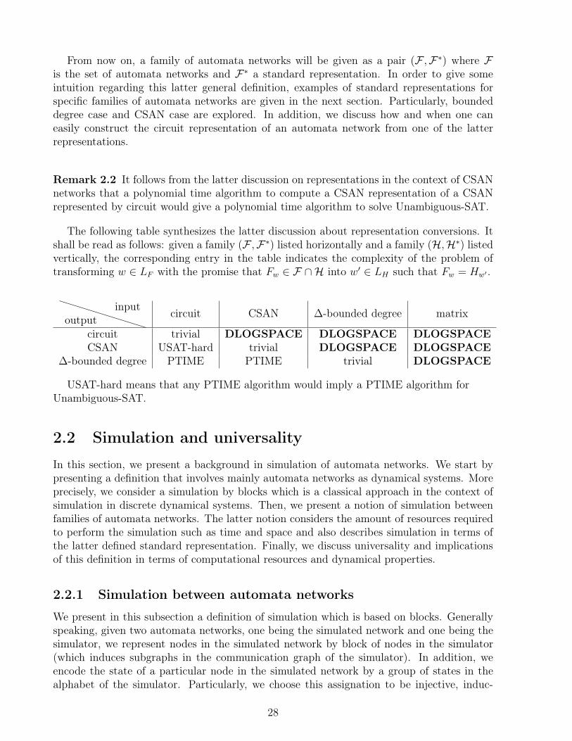
From now on, a family of automata networks will be given as a pair (F ,F⇤) where F

is the set of automata networks and F⇤ a standard representation. In order to give someintuition regarding this latter general definition, examples of standard representations forspecific families of automata networks are given in the next section. Particularly, boundeddegree case and CSAN case are explored. In addition, we discuss how and when one caneasily construct the circuit representation of an automata network from one of the latterrepresentations.

Remark 2.2 It follows from the latter discussion on representations in the context of CSANnetworks that a polynomial time algorithm to compute a CSAN representation of a CSANrepresented by circuit would give a polynomial time algorithm to solve Unambiguous-SAT.

The following table synthesizes the latter discussion about representation conversions. Itshall be read as follows: given a family (F ,F⇤

) listed horizontally and a family (H,H⇤) listed

vertically, the corresponding entry in the table indicates the complexity of the problem oftransforming w 2 LF with the promise that Fw 2 F \H into w0 2 LH such that Fw = Hw0 .

outputinput circuit CSAN �-bounded degree matrix

circuit trivial DLOGSPACE DLOGSPACE DLOGSPACE

CSAN USAT-hard trivial DLOGSPACE DLOGSPACE

�-bounded degree PTIME PTIME trivial DLOGSPACE

USAT-hard means that any PTIME algorithm would imply a PTIME algorithm forUnambiguous-SAT.

2.2 Simulation and universalityIn this section, we present a background in simulation of automata networks. We start bypresenting a definition that involves mainly automata networks as dynamical systems. Moreprecisely, we consider a simulation by blocks which is a classical approach in the context ofsimulation in discrete dynamical systems. Then, we present a notion of simulation betweenfamilies of automata networks. The latter notion considers the amount of resources requiredto perform the simulation such as time and space and also describes simulation in terms ofthe latter defined standard representation. Finally, we discuss universality and implicationsof this definition in terms of computational resources and dynamical properties.

2.2.1 Simulation between automata networks

We present in this subsection a definition of simulation which is based on blocks. Generallyspeaking, given two automata networks, one being the simulated network and one being thesimulator, we represent nodes in the simulated network by block of nodes in the simulator(which induces subgraphs in the communication graph of the simulator). In addition, weencode the state of a particular node in the simulated network by a group of states in thealphabet of the simulator. Particularly, we choose this assignation to be injective, induc-

28

Bi

vi

F

H

Figure 2.1: Scheme of one-to-one block simulation. In this case, network F is simulated byH. Each node in F is assigned to a block in H and state coding is injective. Observe thatblocks are connected (one edge in the original graph may be represented by a path in thecommunication graph of H) according to connections between nodes in the original networkF . This connections are represented by blue lines.

ing certain injective code map. A similar approach was broadly studied in the context ofsimulation between cellular automata [49, 8, 60, 64, 65]. Note that defining an injectivecoding map is not arbitrary. It allows us to avoid problems that could arrive in the con-text of transferring dynamical properties from a simulated network to the simulator suchas, for example, preserving the transient lengths and the attractor periods. In addition, itmakes the notion of simulation compatible with reductions in the context of comparing thecomputational complexity of the prediction problem between the simulator network and thesimulated network.

Definition 2.3 Let F : QVF

F ! QVF

F and H : QVH

H ! QVH

H be automata networks. A blockembedding of QVF

F into QVH

H is a collection of blocks Di ✓ VH for each i 2 VF which formsa partition of VH together with a collection of patterns pi,q 2 QDi

H for each i 2 VF and eachq 2 QF such that pi,q = pi,q0 implies q = q0. This defines an injective map � : QVF

F ! QVH

H by�(x)Di = pi,xi for each i 2 VF . We say that H simulates F via block embedding � if there isa time constant T such that the following holds on QVF

F :

� � F = HT � �.

See Figure 2.1 for a scheme of block simulation. In the following, when useful we representa block embedding as the list of blocks together with the list of patterns. The size of thisrepresentation is linear in the number of nodes (for a fixed alphabet).

Remark 2.4 It is convenient in many concrete cases to define a block embedding throughblocks Di that are disjoint but do not cover VH and add a context block C disjoint from theDi that completes the covering of VH . In this variant a block embedding of QVF

F into QVH

H isgiven by patterns pi,q and a constant context pattern pC 2 QC

H which define an injective map� : QVF

F ! QVH

H by �(x)Di = pi,xi for each i 2 VF and �(x)C = pC . This variant is actually

29

just a particular instance of Definition 2.3 because we can include C in an arbitrary block(Di Di [ C) and define the block embedding as in Definition 2.3.

In our proofs of simulations (see next subsections), the variant blocks/context will beparticularly relevant because the size of blocks will be bounded while the context will growwith the size of the considered automata. Said differently, the information about an encodedstate will be very localized.

Another natural particular case of Definition 2.3 corresponding to localized informationis when in each block Di, there is a special node vi 2 Di such that the map q 7! pi,q(vi) isinjective. It is only possible when QH is larger than QF , but it will be the case in severalexamples of Boolean automata networks (see Chapter 5) . Interestingly, this local codingphenomena is forced when some automata network H simulates some Boolean automatanetwork F : indeed, in any block Di of H at least one node vi must change between patternspi,0 and pi,1, but the map x 2 {0, 1} 7! pi,x being injective, it means that x 7! pi,x(vi) isinjective too.

Remark 2.5 The simulation relation of Definition 2.3 is a pre-order on automata networks.

We now observe that simulation can also be seen in terms of orbit graphs. In this sense,we present the following lemma:

Lemma 2.6 If H simulates F via block embedding with time constant T then the orbit graphGF of F is a subgraph of GT

H . In particular if F has an orbit with transient of length t andperiod of length p, then H has an orbit with transient of length Tt and period Tp.

Proof. The embedding of GF inside GTH is realized by definition by the block embedding of

the simulation. The consequence on the length of periods and transients comes from the factthat the embedding � verifies: x is in a periodic orbit if and only if �(x) is in a periodicorbit.

2.2.2 Simulation between families of automata networks

In this section we present a notion of simulation in terms of representations and the amountof resources that are needed in order to simulate a certain family of automata networks bysome other arbitrary family. Roughly speaking, a family of automata network can simulatea particular automata network if we are able to effectively construct some automata networkin this collection that is able to simulate the first automata network in the sense of the latterdefinition of simulation. More precisely, we ask the automata network which performs thesimulation to do this task in reasonable time and reasonable space in a sense that we specifyin the next definition.

Definition 2.7 Let (F ,F⇤) and (H,H⇤

) be two families with standard representations onalphabets QF and QH respectively. Let T, S : N ! N be two functions. We say that F⇤

30

simulates H⇤ in time T and space S if there exists a DLOGSPACE Turing machine Msuch that for each w 2 LH representing some automata network Hw 2 H : Qn

H ! QnH , the

machine produces a pair M(w) which consists in:

• w0 2 LF with Fw0 : QnF

F ! QnF

F ,• a representation of a block embedding � : QnF ! Qn,

such that nF = S(n) and Fw0 simulates Hw in time T = T (n) under block embedding �.

From now on, whenever F⇤ simulates H⇤ in time T and space S we write H⇤ 4TS F⇤.

Remark 2.8 The simulation relation between families is transitive because the classDLOGSPACE is closed under composition and simulation between individual automatanetworks is also transitive. When composing simulations time and space maps S and T getmultiplied.

2.3 Decision problems and automata network dynamicsIn this section we introduce three variants of a classical decision problem that is closelyrelated to the dynamical behavior of automata networks: the prediction problem. Thisproblem consists in predicting if one node of the network will change its state at given time.We study first a short term version of the problem in which time is given in the input. Inaddition, we explore a stronger variant of this problem in which we ask if some node haseventually changed, provided a constant observation time rate ⌧ . In other words, we checkthe system for any change on the state of a particular node every multiple of ⌧ time steps.Finally, we conclude that these problems are coherent with our simulation definition in thesense that if some family of automata networks (F2,F⇤

2) simulates (F1,F⇤

1) then, if some of

the latter problem is hard in some sense for F1 it will also be hard for F 02. We will precise

this result in the following lines.

Let (F ,F⇤) be an automata network family and let L 2 {0, 1}⇤⇥{0, 1}⇤ be a parameterized

language. We say that L is parameterized by F if L has F⇤ encoded as parameter. We noteLF ✓ {0, 1}⇤ as the language resulting on fixing F⇤ as a constant.

In particular, we are interested in studying prediction problems. We start by defining twovariants of this well-known decision problem:

Problem (Unary Prediction (PREDu))

Parameters: alphabet Q, a standard representation F⇤ of an automata network family F

Input:

1. a word wF 2 F⇤ representing an automata network F : Qn ! Qn with F 2 F .2. a node v 2 V (F ) = {1, . . . , n}

31

3. an initial configuration x 2 QV .4. a natural number t represented in unary such that t 2 1.

Question: F t(x)v 6= xv?

Problem (Binary Prediction (PREDb))

Parameters: alphabet Q, a standard representation F⇤ of an automata network family F

Input:

1. a word wF 2 F⇤ representing an automata network F : Qn ! Qn with F 2 F .2. a node v 2 V (F ) = [n]

3. an initial configuration x 2 QV .4. a natural number t represented in binary t 2 {0, 1}⇤.

Question: F t(x)v 6= xv?

Note that two problems are essentially the same, the only difference is the representationof time t that we call the observation time. We will also call node v the objective node.As it happens with other decision problems, such as integer factorization, the representationof observation time will have an impact on the computation complexity of the predictionproblem. When the context is clear we will refer to both problems simply as PRED. Observethat one can always solve the prediction problem by simply computing F t

(x) in order toverify if F t

(x)v 6= xv. Thus, since F is deterministic, we have that PREDuF 2 P andPREDbF 2 PSPACE.

Finally, we show that latter problem is coherent with our definition of simulation, in thesense that we can preserve the complexity of PRED. Note that this gives us a powerful toolin order to classify concrete automata rules according to the complexity of the latter decisionproblem.

Lemma 2.9 Let (F ,F⇤) and (H,H⇤

) be two automata network families. Let T, S : N! Nbe two polynomial functions such that H⇤ 4T

S F⇤ then, PREDH⇤ TL PREDF⇤

1

Proof. Let (wH , v, x, t) be an instance of PREDH⇤ . By definition of simulation, there existsa DLOGSPACE algorithm which takes wH and produces a word wF 2 LF with F : QnF !QnF and a block representation � : QnF ! Qn such that nF = S(n) and F simulates H in timeT (n) under block embedding �. Particularly, there exists a partition of blocks Dv ✓ V (F ) =

[nF ] for each v 2 V (H) = [n] and a collection of injective patterns, i.e. patterns pi,q 2 QDiF

such that pi,q = pi,q0 =) q = q0. In addition, we have � � H = F T � �. Let us define theconfiguration y 2 QnF

F as yDi = pi,xi , i.e., �(x)Di = yDi . Note that y is well-defined as the blockmap is injective. In addition, let us choose an arbitrary vertex v0 2 Dv and let us consider

1Here we denote TL as a DLOGSPACE Turing reduction. The capital letter “T” stands for Turing

reduction and it is not related to the simulation time function which is also denoted by T.

32

now the instance of PREDF⇤ given by (wF , v0, y, t ⇥ T ). Note that for each v0 2 Dv thetransformation (wH , v, x, t)! (wF , v0, y, t⇥T ) can be done in DLOGSPACE(|wH |) becausewe can read the representation of � for each block pi,xi and then output the configuration y.We claim that there exists a DLOGSPACE(|wH |) algorithm that decides if (wH , v, x, t) 2LPREDH⇤ with oracle calls to PREDF⇤ . More precisely, as a consequence of the injectivityof block embedding, we have that (wH , v, x, t) 2 LPREDH⇤ if and only if (wF , v0, y, t ⇥ T ) 2LPREDF⇤ for some v0 2 Dv. In fact, the latter algorithm just runs oracle calls of PREDF⇤

for (wF , v0, y, t⇥T ) for each v0 2 Dv and decides if some of these instances is a YES instanceand thus, if some node in the simulation block have changed its state. As block-embeddingis injective, this necessary means that node v have changed its state in t time steps. Finally,all of this can be done in DLOGSPACE since nF = S(n) = nO(1) and T = nO(1) and thus,a polynomial amount of calls to each oracle is needed.

Finally, we would like to study the case in which time is not part of the entry of PRED.In other words, we would like to observe the long-term dynamical behavior of the objectivenode. However, in order to preserve complexity properties under simulation, we still needto have some sort of observation gap as a part of the entry of PRED. This will allow usto avoid giving misleading answers when the simulating network is performing one step ofsimulation. We recall that it could take several time steps for the simulating network in orderto represent one step of the dynamics of the simulated network. In order to manage this sortof time dilatation phenomenon between simulating and simulated systems, we introduce thefollowing decision problem:

Problem (Prediction change PREDcF⇤)

Parameters: alphabet Q, a standard representation F⇤ of an automata network family F .

Input:

1. a word wF 2 F⇤ representing an automata network F : QV ! QV with F 2 Fand V = {1, . . . , n}.

2. a node v 2 V

3. an initial configuration x 2 QV .4. a time gap k 2 1

Question: 9t 2 N : F kt(x)v 6= xv

Observe that, again, the latter decision problem can be solved in PSPACE by directcomputation of F kt

(x) for different values of t until the orbit reaches an attractor. For eacht, it is possible to very if objective node has eventually changed or not. Now we show that thecomputational complexity of the latter problem is consistent under our notion of simulation.

Lemma 2.10 Let (F ,F⇤) and (H,H⇤

) be two automata network families and T, S : N! Ntwo polynomial functions such that H⇤ 4T

S F⇤ then, PREDcH⇤ TL PREDcF⇤.

33

Proof. The proof is analogous to short term prediction case. Let (wH , v, x) be an instanceof PREDH⇤ . Again, by the definition of simulation, there exists a DLOGSPACE algo-rithm which takes wH and produces a word wF 2 LF with F : QnF ! QnF and a blockrepresentation � : QnF ! Qn such that nF = S(n) and F simulates H in time T (n) underblock embedding �. The latter statements means, particularly, that there exists a partitionof blocks Dv ✓ V (F ) = [nF ] for each v 2 V (H) = [n] and a collection of injective patterns,i.e. patterns pi,q 2 QDi

F such that pi,q = pi,q0 =) q = q0 and also that � �H = F T � �. Letus define the configuration y 2 QnF

F as yDi = pi,xi , i.e., �(x)Di = yDi . Note, again, that yis well-defined as the block map is injective. Now we proceed by using the same approachthan before: for each v0 2 Dv we can produce an instance (wF , v0, y) of PREDcF⇤ . Then,as T and S are polynomials, there exists an oracle DLOGSPACE machine which produces(wF , v0, y) for each v0 2 Dv and calls for an oracle PREDcF⇤(wF , v0, y). Then, algorithmverifies whether there is a YES-instance for some v0. By definition of simulation and in-jectivity of block embedding function we have that this algorithm outputs 1 if and only if(wH , v, x) 2 PREDH⇤ .

2.4 Universal automata network familiesIn the next lines, we will give the definition of a universal family of automata networks. Insimple words, a universal family is a set of automata networks which is able to simulate everyother automata network. Of course, in this context, we precise the amount of resources thatsome family will need in order to simulate an arbitrary automata network by controlling func-tions S and T (otherwise we could take families that use an enormous amount of resources assimulators). In addition, it is important to remark again the essential role of representations.When we say that some family can simulate every other family, we have to be careful withthe fact that, as we are choosing mainly circuits as a representation for automata networks,the size of a circuit which simulates certain automata network could be exponential in thesize of the network. Thus, as we are going to use the circuit as a main construction block inthe process of constructing a simulator, this latter observation will have an important role inthe moment to express the properties of the simulator in terms of the simulated network. Inorder to avoid this issue, we are very specific in the notion of universal family of automatanetworks by adding a constraint in the size of the circuit representing an automata networkin this family.

Building upon our definition of simulation, we can now define a precise notion of universal-ity. In simple words, a universal family is one that is able to simulate every other automatanetwork under any circuit encoding. Our definition of simulation ensures that the amount ofresources needed in order to simulate is controlled so that we can deduce precise complexityresults.

Consider some alphabet Q and some polynomial map P : N! N. We denote by UQ,P theclass of all possible functions F : Qn ! Qn for any n 2 N that admits a circuit representationof size at most P (n). We also denote U⇤

Q,P the language of all possible circuit representationsof size bounded by P of all functions from UQ,P . Finally for any � � 1, denote by BQ,� theset of automata networks on alphabet Q with a communication graph of degree bounded by� and by B⇤

Q,� their associated bounded degree representations made of a pair (graph, localmaps) as discussed above.

34

Definition 2.11 A family of automata networks (F ,F⇤) is :

• universal if for any alphabet Q and any polynomial map P it can simulate (UQ,P ,U⇤Q,P )

in time T and space S where T and S are polynomial functions;• strongly universal if for any alphabet Q and any degree � � 1 it can simulate (BQ,�,B⇤

Q,�)

in time T ans space S where T and S are linear maps.

Remark 2.12 The link between the size of automata networks and the size of their repre-sentation is the key in the above definitions. A universal family must simulate any individualautomata network F (just take P large enough so that F 2 UQ,P ). However it is not re-quired to simulate in polynomial space and time a family of networks whose smallest circuitrepresentations are super-polynomial. Actually no family admitting polynomial circuit rep-resentation could simulate such a super-polynomial family in polynomial time and space. Inparticular the family BQ,� cannot.

At this point it is clear, by transitivity of simulations, that if some BQ,� happens to beuniversal then, any strongly universal family is also universal. It turns out that B{0,1},3 isuniversal. We will however delay the proof until Chapter 3 where we prove a more preciseresult which happens to be very useful to get universality result in concrete families.

Now, we introduce an important corollary of universality regarding complexity. Roughlyspeaking, a universal family exhibits all the complexity in terms of dynamical behavior andcomputational complexity of prediction problems. Concerning computational complexity, letus introduce the following definition.

Definition 2.13 We say that an automata network family F is computationally complex ifthe following conditions hold:

1. PREDuF is P-hard.2. PREDbF is PSPACE-hard.3. PREDcF is PSPACE-hard.

As a direct consequence of universality, we have the following result where there is nodifference between strong or standard universality.

Corollary 2.14 Let F be a (strongly) universal automata network family. Then, F compu-tationally complex.

Proof. We show that there exists a bounded degree automata network family which is dy-namically complex. Then, any universal family will also satisfy each of latter properties asa direct consequence of the simulation. In fact, we cite a classical result in simulation ofTuring Machines by elementary cellular automata [57] in which it is shown that it is possibleto simulate an arbitrary Turing Machine with n states and m symbols in space O(n + m)

and in twice linear time. This is accomplished by adding two auxiliary states which decou-

35

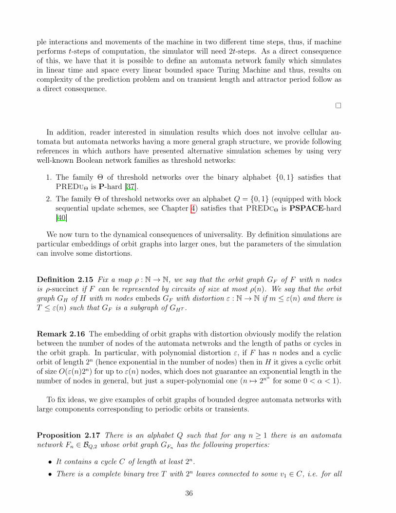
ple interactions and movements of the machine in two different time steps, thus, if machineperforms t-steps of computation, the simulator will need 2t-steps. As a direct consequenceof this, we have that it is possible to define an automata network family which simulatesin linear time and space every linear bounded space Turing Machine and thus, results oncomplexity of the prediction problem and on transient length and attractor period follow asa direct consequence.

In addition, reader interested in simulation results which does not involve cellular au-tomata but automata networks having a more general graph structure, we provide followingreferences in which authors have presented alternative simulation schemes by using verywell-known Boolean network families as threshold networks:

1. The family ⇥ of threshold networks over the binary alphabet {0, 1} satisfies thatPREDu⇥ is P-hard [37].

2. The family ⇥ of threshold networks over an alphabet Q = {0, 1} (equipped with blocksequential update schemes, see Chapter 4) satisfies that PREDc⇥ is PSPACE-hard[40]

We now turn to the dynamical consequences of universality. By definition simulations areparticular embeddings of orbit graphs into larger ones, but the parameters of the simulationcan involve some distortions.

Definition 2.15 Fix a map ⇢ : N! N, we say that the orbit graph GF of F with n nodesis ⇢-succinct if F can be represented by circuits of size at most ⇢(n). We say that the orbitgraph GH of H with m nodes embeds GF with distortion " : N! N if m "(n) and there isT "(n) such that GF is a subgraph of GHT .

Remark 2.16 The embedding of orbit graphs with distortion obviously modify the relationbetween the number of nodes of the automata netwroks and the length of paths or cycles inthe orbit graph. In particular, with polynomial distortion ", if F has n nodes and a cyclicorbit of length 2

n (hence exponential in the number of nodes) then in H it gives a cyclic orbitof size O("(n)2n) for up to "(n) nodes, which does not guarantee an exponential length in thenumber of nodes in general, but just a super-polynomial one (n 7! 2

n↵ for some 0 < ↵ < 1).

To fix ideas, we give examples of orbit graphs of bounded degree automata networks withlarge components corresponding to periodic orbits or transients.

Proposition 2.17 There is an alphabet Q such that for any n � 1 there is an automatanetwork Fn 2 BQ,2 whose orbit graph GFn

has the following properties:

• It contains a cycle C of length at least 2n.• There is a complete binary tree T with 2

n leaves connected to some v1 2 C, i.e. for all

36

v 2 T there is a path from v to v1.• There is a node v2 2 C with a directed path of length 2

n pointing towards v2.

Proof. First on a component of states {0, 1, 2} ✓ Q the large cycle C is obtained by thefollowing ”odometer” behavior of Fn: if xn 2 {0, 1, 2} then Fn(x)n = xn + 1 mod 3, and ifboth xi, xi+1 2 {0, 1, 2} for 1 i < n then

Fn(x)i =

8><

>:

0 if xi = 2,xi + 1 else if xi+1 = 2,

xi else.

C is realized on {0, 1, 2}n as follows. For x 2 {0, 1, 2}n we denote by Si the sequence(F t

(x)i)t�0 for any 1 i n. Clearly Sn is periodic of period 012. Sn�1 is ultimately periodicof period 200111 (of length 6) and by a straighforward induction we get that S1 is ultimatelyperiodic of period 20

3·2n�2�113·2n�2 which is of length 3 · 2n�1.

For the tree T , just add states {a, b} ✓ Q with the following behavior: if x1 2 {a, b} thenFn(x)1 = 0 and if xi 2 {a, b} and xi�1 = 0 then Fn(x)i = 0 for 1 < i n. In any other case,we set F (x)i = xi for x 2 {0, 1, 2, a, b}n and 1 i n.

Finally, using similar mechanisms as above on additional states c0, c1, c2 2 Q, Fn runsanother odometer whose behavior is isomorphic to the behavior of Fn on {0, 1, 2}n throughi 7! ci, but with the following exception: when x1 = c2 we set Fn(x)1 = 0 and then state 0

propagates from node 1 to node n as in the construction of tree T . We thus get a transientbehavior of length more than 3 · 2n�1 which yields to configuration 0

n, which itself (belongsor) yields to cycle C.

Now we can now state that any universal family must be dynamically rich in a precisesense.

Theorem 2.18 Let F be an automata networks family.

• If F is universal then, for any polynomial map ⇢, there is a polynomial distortion "such that, any ⇢-succinct orbit graph can be embedded into some F 2 F with distortion". In particular F contains networks with super-polynomial periods and transients.

• If F is strongly universal then it embeds the orbit graph of any bounded-degree automatanetwork with linear distortion. In particular it contains networks with exponential pe-riods and transients.

Proof. This is a direct consequence of Lemma 2.6, Definition 2.7 and Proposition 2.17 above.

In a directed graph, we say that a node v belongs to a strongly connected component ifthere is a directed path from v to v.

37

Corollary 2.19 Any universal family F satisfies the following: there is a constant ↵ with0 < ↵ 1 such that for any m > 0 there is a network F 2 F with n � m nodes such thatthere exists some node v belonging to a strongly connected component of the interaction graphof F and a periodic configuration x such that the trace at v of the orbit of x is of period atleast 2n↵.

Proof. Consider a Boolean network F with n nodes numbered by {1, . . . , n} that does thefollowing on configuration x: it interprets x1, . . . , xn as a number k written in base 2 where x1

is the most significant bit and define F (x) so that F (x)x1,...,xnrepresents number k + 1 mod 2

n

with node 1 holding the most significant bit. F is such that node 1 has trace of exponentialperiod in some periodic orbit and it is in a strongly connected component since it dependson itself. Note that F has a circuit representation which is polynomial in n, and takeF 0 2 F of polynomial size in n that simulates F in polynomial time. Taking the notationsof Definition 2.3, we have that each node v 2 Di for each block Di is such that the mapq 2 {0, 1} 7! pi,q(v) is either constant or bijective (because F has a Boolean alphabet, seeRemark 2.4). In the last case, the value of the node v 2 Di completely codes the value ofthe corresponding node i in F . Take any v 2 B1 that has this coding property. Since node1 depends on itself in F , there must be a path from v to some coding node v0 2 D1. Then,again, as node 1 depends on itself in F , there must be a path from v0 to some coding nodein D1. Iterating this reasoning we must find a cycle, and in particular we have a codingnode in D1 which belongs to some strongly connected component of the interaction graph ofF 0. Since this node is coding the values taken by node 1 of F and since the simulation is inpolynomial time and space, we deduce the super-polynomial lower bound on the period ofits trace for a well-chosen periodic configuration.

38

Chapter 3

Gadget complexity: from local to globalbehavior

3.1 Putting pieces together: glueing automata networks

In this section we define an operation that allows us to ”glue” two different abstract automatanetworks on a common part in order to create another one which, preserve some dynamicalproperties in the sense that it allows to glue pseudo-orbits of each network to obtain a pseudo-orbit of the glued network. One might find useful to think about the common part of thetwo networks as a dowel attaching two pieces of wood: each individual network is a piece ofwood with the dowel inserted in it, and the result of the glueing is the attachment of the twopieces with a single dowel (see Figure 3.1). The idea is that, in this scheme, each node in theglued network will dynamically behave as same as a node in the first network or as a nodein the second network.

Definition 3.1 Consider F1 : QV1 ! QV1 and F2 : QV2 ! QV2 two automata networks withV1 disjoint from V2, C a set disjoint from V1 [ V2, '1 : C ! V1 and '2 : C ! V2 two injectivemaps and C1, C2 a partition of C in two sets. We define

V 0= C [ (V1 \ '1(C)) [ (V2 \ '2(C))

and the map ↵ : V 0 ! V1 [ V2 by

↵(v) =

(v if v 62 C

'i(v) if v 2 Ci, for i = 1, 2.

We then define the glueing of F1 and F2 over C as the automata network F 0: QV 0 ! QV 0

where

F 0v =

((F1)↵(v) � ⇢1 if ↵(v) 2 V1,

(F2)↵(v) � ⇢2 if ↵(v) 2 V2,

39

C

'1(C) '2(C)

V1

V2

'1 '2

C

V 0

Figure 3.1: General scheme of a glueing.

where ⇢i : QV 0 ! QVi is defined by

⇢i(x)v =

(x'�1

i (v) if v 2 'i(C),

xv else.

When necessary, we will use the notation F 0= F1

�1C1��2

C2F2 to underline the dependency

of the glueing operation on its parameters.

Given an automata network F : QV ! QV and a set X ✓ V , we say that a sequence(xt

)0tT of configurations from QV is a X-pseudo-orbit if it respects F as in a normal orbit,except on X where it can be arbitrary, formally: xt+1

v = F (xt)v for all v 2 V \X and all

0 t < T . The motivation for Definition 3.1 comes from the following lemma.

Lemma 3.2 (Pseudo-orbits glueing) Taking the notations of Definition 3.1, letX ✓ V1 \ '1(C) and Y ✓ V2 \ '2(C) be two (possibly empty) sets. If (xt

)0tT is aX [ '1(C2)-pseudo-orbit for F1 and if (yt)0tT is a Y [ '2(C1)-pseudo-orbit for F2 andif they verify for all 0 t T that:

8v 2 C, xt'1(v) = yt'2(v), (3.1)

then the sequence (zt)0tT of configurations of QV 0 is a X [ Y -pseudo-orbit of F 0, where

ztv =

(xt↵(v) if ↵(v) 2 V1,

yt↵(v) if ↵(v) 2 V2.

Proof. Take any v 2 V 0 \ (X [ Y ). Suppose first that ↵(v) 2 V1. By definition of F 0, wehave F 0

(zt)v = (F1)↵(v) � ⇢1(zt) but ⇢1(zt) = xt (using the Equation 3.1 in the hypothesis) so

40

+ =

�1(C1)

�1(C2)

�2(C1)

�2(C2)

Figure 3.2: Symmetry breaking in interaction graph after a glueing operation. Arrows in-dicate influence of a node (source) on another (target), edges without arrow indicates bi-directional influence. Here C consists in two nodes only.

F 0(zt)v = F1(xt

)↵(v). Since (xt) is a X [ '1(C2)-pseudo-orbit and since ↵(v) 62 X [ '1(C2),

we haveF1(x

t)↵(v) = xt+1

↵(v) = zt+1

v .

We conclude that zt+1

v = F 0(zt)v. By a similar reasoning, we obtain the same conclusion if

↵(v) 2 V2. We deduce that (zt) is a X [ Y -pseudo-orbit of F 0.

In the case of a CSAN family where the transition rules are determined by a labeled non-directed graph, the result of a glueing operation has no reason to belong to the family becausethe symmetry of the interaction graph might be broken (see Figure 3.2). The following lemmagives a sufficient condition in graph theoretical terms for glueing within a CSAN family.Intuitively, it consists in asking that, in each graph, all the connections of one half of thedowel to the rest of the graph goes through the other half of the dowel. Here the woodendowel metaphor is particularly relevant: when considering a single piece of wood with thedowel inserted in it, one half of the dowel is ”inside” (touches the piece of wood), the otherhalf is ”outside” (not touching the piece of wood); then, when the two pieces are attached,each position in the wood assembly is locally either like in one piece of wood with the dowelinserted in it or like in the other one with the dowel inserted in it.

Lemma 3.3 (Glueing for CSAN) Let (G1,�1, ⇢1) and (G2,�2, ⇢2) be two CSAN from thesame CSAN family F where G1 and G2 are disjoint and F1 and F2 are the associated globalmaps. Taking again the notations of Definition 3.1, if the following conditions hold:

• the labeled graphs induced by '1(C) and '2(C) in G1 and G2 are the same (using theidentification '1(v) = '2(v));

• NG1('1(C2)) ✓ '1(C); and• NG2('2(C1)) ✓ '2(C);

then the glueing F 0= F1

�1C1��2

C2F2 can be defined as the CSAN on graph G0

= (V 0, E 0) where

V 0 is as in Definition 3.1 and each node v 2 V 0 has the same label and same labeled neigh-borhood as either a node of (G1,�1, ⇢1) or a node of (G2,�2, ⇢2). In particular F 0 belongs toF .

41

Proof. Let us define �i : Vi ! V 0 by

�i(v) =

(��1

i(v) if v 2 �i(C),

v else.

Fix i = 1 or 2. According to Definition 3.1, if v 2 V 0 is such that ↵(v) 2 Vi thenF 0v = (Fi)↵(v) � ⇢i. By definition of CSAN, this means that for any x 2 QV 0 we have

F 0v(x) = i,↵(v)(x|�(NGi

(↵(v)))) where i,↵(v) is a map depending only on the labeled neigh-borhood of ↵(v) in Gi as in Definition 1.5. So the dependencies of v in F 0 are in one-to-onecorrespondence through � with the neighborhood of ↵(v) in Gi. The key observation is thatthe symmetry of dependencies is preserved, formally for any v0 2 �(NGi(↵(v))):

• either ↵(v0) 2 Vi in which case the dependency of v0 on v (in map i,↵(v0)) is the same asthe dependency of v on v0 (in map i,↵(v)), and both are determined by the undirectedlabeled edge {↵(v),↵(v0)} of Gi;

• or ↵(v0) 62 Vi and in this case necessarily v 2 Ci and v0 2 C3�i (becauseNGi(Vi \ 'i(C)) \ 'i(C) ✓ 'i(Ci) from the hypothesis), so the dependency of v0 on vis the same as the dependency of v on v0 because the labeled graphs induced by �1(C)

and �2(C) in G1 and G2 are the same.

Concretely, F 0 is a CSAN that can be defined on graph G0= (V 0, E 0

1[ E 0

2[ E(C)) with

E 0i= E(Vi \ 'i(C)) [ {(u, vi) : u 2 V (Ci), vi 2 (Vi \ 'i(C)), ('i(u), vi) 2 Ei},

and labels as follows:

• on E(C) as in both G1 and G2 (which corresponds to the image of maps �1 and �2 onC);

• on E(Vi \ 'i(C)) as in Gi;• for each u 2 V (Ci), vi 2 (Vi \ 'i(C)) such that ('i(u), vi) 2 Ei, edge (u, vi) has same

label as ('i(u), vi);

Since any CSAN families (Definition 1.5) is entirely based on local constraints on labels(vertex label plus set of labels of the incident edges), we deduce that F 0 is in F .

3.2 Computing on automata networks

3.2.1 G-networks

In this subsection, we formalize the idea of building large automata networks from smallbuilding blocks. By building blocks, we mean any finite maps with some number of inputsand some number of outputs that all share the same alphabet. It can be helpful to thinkabout Boolean automata networks built from Boolean gates. However, in our formalism, fanin and fan out are not free (they are allowed if available as a building block). These detailsare important since neither information duplication, neither synchronization are granted inour context of embedding computations into dynamical systems.

42

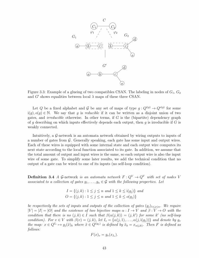
a b c b c

d

e

e

d

cb

C1 C2

a

G1G2

G0

C

'1 '2

Figure 3.3: Example of a glueing of two compatibles CSAN. The labeling in nodes of G1, G2

and G0 shows equalities between local � maps of these three CSAN.

Let Q be a fixed alphabet and G be any set of maps of type g : Qi(g) ! Qo(g) for somei(g), o(g) 2 N. We say that g is reducible if it can be written as a disjoint union of twogates, and irreducible otherwise. In other terms, if G is the (bipartite) dependency graphof g describing on which inputs effectively depends each output, then g is irreducible if G isweakly connected.

Intuitively, a G-network is an automata network obtained by wiring outputs to inputs ofa number of gates from G. Generally speaking, each gate has some input and output wires.Each of these wires is equipped with some internal state and each output wire computes itsnext state according to the local function associated to its gate. In addition, we assume thatthe total amount of output and input wires is the same, so each output wire is also the inputwire of some gate. To simplify some later results, we add the technical condition that nooutput of a gate can be wired to one of its inputs (no self-loop condition).

Definition 3.4 A G-network is an automata network F : QV ! QV with set of nodes Vassociated to a collection of gates g1, . . . , gn 2 G with the following properties. Let

I = {(j, k) : 1 j n and 1 k i(gj)} andO = {(j, k) : 1 j n and 1 k o(gj)}

be respectively the sets of inputs and outputs of the collection of gates (gj)1jn. We require|V | = |I| = |O| and the existence of two bijective maps ↵ : I ! V and � : V ! O with thecondition that there is no (j, k) 2 I such that �(↵(j, k)) = (j, k0

) for some k0 (no self-loopcondition). For v 2 V with �(v) = (j, k), let Iv = {↵(j, 1), . . . ,↵(j, i(gj))} and denote by gvthe map: x 2 QIv 7! gj(x)k where x 2 Qi(gj) is defined by xk = x↵(j,k). Then F is defined asfollows:

F (x)v = gv(xIv).

43

g1

(1, 1)

(1, 1) (1, 2)

�A

g2

(2, 1)

(2, 1) (2, 2)

�B �C

g1

g2

AB C

AB C

(2,1) (1,1)(1,1) (2,1) (1,2) (2,2)

8><

>:

�(x)A = �A(xB, xC)

�(x)B = �B(xA)

�(x)C = �C(xA)

Figure 3.4: (Left panel) A set of maps G over alphabet Q. (Central panel) An intuitiverepresentation of input/output connections to make a G-network. (Right panel) The corre-sponding formal G-network � : Q3 ! Q3 together with the global map associated to it. Thebijections ↵ and � from Definition 3.4 are represented in blue and red (respectively).

Remark 3.5 Once G is fixed, there is a bound on the degree of dependency graphs of allG-networks. Thus, it is convenient to represent G-networks by the standard representationof bounded degree automata networks (as a pair of a graph and a list of local update maps).Another representation choice following strictly Definition 3.4 consists in giving a list ofgates g1, . . . , gk 2 G, fixing V = {1, . . . , n} and give the two bijective maps ↵ : I ! V and� : V ! O describing the connections between gates (maps are given as a simple list of pairssource/image). One can check that these two representations are DLOGSPACE equivalentwhen the gates of G are irreducible: we can construct the interaction graph and the localmaps from the list of gates and maps ↵ and � in DLOGSPACE (the incoming neighborhoodof a node v, Iv, and its local map gv are easy to compute as detailed in Definition 3.4);reciprocally, given the interaction graph G and the list of local maps (gv), one can recover inDLOGSPACE the list of gates and their connections as follows:

• for v from 1 to n do:– gather the (finite) incoming neighborhood N�

(v) of v then the (finite) outgoingneighborhood N+

(N�(v)) and iterate this process until it converges (in finite time)

to a set Iv of inputs and Ov of outputs with v 2 Ov;– check that all v0 2 Ov are such that v0 � v otherwise jump to next v in the loop

(this guaranties that each gate is generated only once);– since the considered gates are irreducible, Iv and Ov actually correspond to input

and output sets of a gate g 2 G that we can recover by finite checks from the localmaps of nodes in Ov;

– output gate g and the pairs source/image to describe ↵ and � for nodes in Iv andOv respectively.

For example, in Figure 3.4, right panel, the latter algorithm executes the following instruc-

44

tions:

• For v = A :

– Compute: N�({A}) = {B,C} 7! N+

({B,C}) = {A} 7! N+({A}) = {B,C}.

– Define IA = {B,C} and OA = {A}.– Check that for all v0 2 OA we have v0 � v.

– Define g1 with two inputs labeled as {B,C} and one output labeled by {A} whereg1 ⌘ �A.

• For v = B :

– Compute: N�({B}) = {A} 7! N+

({A}) = {B,C} 7! N+({B,C}) = {A}.

– Define IB = {A} and OB = {B,C}.– Check that for all v0 2 OA we have v0 � v.

– Define g2 with one input labeled as {A} and two outputs labeled by {B,C} whereg2 ⌘ �B.

• For v = C :

– Compute: N�({C}) = {A} 7! N+

({A}) = {B,C} 7! N+({B,C}) = {A}.

– Define IC = {A} and OC = {B,C}.– Check that for all v0 2 OA we have v0 � v. 7! SKIP because B was visited before.

• Return (g1, g2) and its labels.

In the sequel we denote �(G) the family of all posible G-networks associated to theirbounded degree representation.

3.2.2 G-gadgets and simulation of G-networks

Now we give a precise meaning to the intuitively simple fact that, if a family of automatanetworks can coherently simulate a set of small building blocks (gates from G), it should beable to simulate any automata network that can be built out of them (G-networks).

The key idea here is that gates from G will be represented by networks of the familycalled G-gadgets, and the wiring between gates to obtain a G-network will translate intoglueing between G-gadgets. Following this idea there are two main conditions for the familyto simulate any G-network:

• The glueing of gadgets should be freely composable inside the family to allow thebuilding of any G-network.

• The gadgets corresponding to gates from G should correctly and coherently simulatethe functional relation between inputs and outputs given by their corresponding gate.

For clarity, we separate these conditions in two definitions. Concerning glueing, as we wantto mimic the wiring of gates which connects inputs to outputs, several copies of particularsubgraphs will be identified in each gadget, some of them corresponding to input, and theother ones to outputs. Then, the only glueing operations we will use are those where someoutput of a gadget A are glued on input dowels of a gadget B and some inputs of A are gluedon output of B.

45

In order to accomplish that, we introduce in the following section a general framework onglueing gadgets.

3.2.3 Gadget glueing

Now we focus in developing a definition for gadget glueing. Recall first that Definition 3.1relies on the identification of a common dowel in the two networks to be glued. Here, aswe want to mimic the wiring of gates which connects inputs to outputs, several copies ofan interface dowel will be identified in each gadget, some of them corresponding to input,and the other ones to outputs. In this context, the only glueing operations we will use arethose where some output dowels of a gadget A are glued on input dowels of a gadget B andsome input dowels of A are glued on output dowels of B. Then, the global dowel used toformally apply Definition 3.1 is a disjoint union of the selected input/output interface dowels(see Figure 3.5).

Definition 3.6 (Glueing interface and gadgets) Let C = Ci [ Co be a fixed set parti-tioned into two sets. A gadget with glueing interface C = Ci [ Co is an automata networkF : QVF ! QVF together with two collections of injective maps �i

F,k : C ! VF for k 2 I(F )

and �oF,k : C ! VF for k 2 O(F ) whose images in VF are pairwise disjoint and where I(F )

and O(F ) are disjoint sets which might be empty.

Given two disjoint gadgets (F, (�i

F,k), (�oF,k)) and (G, (�i

G,k), (�oG,k)) with same alphabet and

interface C = Ci [ Co, a gadget glueing is a glueing of the form H = F �F

CF��G

CGG defined as

follows:

• a choice of a set A of inputs from F and outputs from G given by injective maps�F : A! I(F ) and �G : A! O(G);

• a choice of a set B of outputs from F and inputs from G given by injective maps⌧F : B ! O(F ) and ⌧G : B ! I(G) (the set B is disjoint from A);

• CF is a disjoint union of |A| copies of Ci, and |B| copies of Co: CF = A⇥ Ci [B ⇥ Co;• CG is a disjoint union of |A| copies of Co, and |B| copies of Ci: CG = A⇥ Co [B ⇥ Ci;• �F : CF [ CG ! VF is such that �F (a, c) = �i

F,�F (a)(c) for a 2 A and c 2 C, and�F (b, c) = �o

F,⌧F (b)(c) for b 2 B and c 2 C; and• �G : CF [ CG ! VG is such that �G(a, c) = �o

G,�G(a)(c) for a 2 A and c 2 C, and�G(b, c) = �i

G,⌧G(b)(c) for b 2 B and c 2 C.

The resulting network H is a gadget with same alphabet and same interface withI(H) = I(F ) \ �F (A) [ I(G) \ ⌧G(B) and O(H) = O(F ) \ ⌧F (B) [O(F ) \ �G(A) and �i

H,k is�i

F,k when k 2 I(F ) and �i

G,k when k 2 I(G), and �oH,k is �o

F,k when k 2 O(F ) and �oG,k when

k 2 O(G).

Given a set of gadgets X with same alphabet and interface, its closure by gadget glueingis the closure of X by the following operations:

• add a disjoint copy of some gadget from the current set;• add the disjoint union of two gadgets from the current set; and

46

inputs outputs

F

�F (A)

⌧F (B)

↵ �

� �

" ⇣

�G(B)

⌧G(A)

G

a b

c d

e f

G

c d

f e

a b

F↵ �

� �

⇣ "

input output

c � � �

f "

a b

Figure 3.5: Gadget glueing as in Definition 3.6. (Left panel) Two gadgets with interfaceC = Ci [ Co where Ci part in each copy of the interface dowel is in red and Co part in blue.The gadget glueing is done with input �F (A) on output �G(A) (here A is a singleton) andoutput ⌧F (B) on input ⌧G(B) (B is also a singleton). (Top right panel) A representation ofthe global glueing process where nodes in green are those in the copy of CF in F or in thecopy CG in G; dotted links show the bijection between the embeddings of C = CF [ CG intoVF and VG via maps �F and �G. (Bottom right panel) The resulting gadget with the sameinterface C = Ci [ Co as the two initial gadgets.

• add a gadget glueing of two gadgets from the current set.

Remark 3.7 The representation of the result of a gadget glueing can be easily computedfrom the two gadgets F and G and the choices of inputs/outputs given by maps �F , �G, ⌧Fand ⌧G: precisely, by definition of glueing (Definition 3.1) the local map of each node of theresult automata network is either a local map of F (when in VF \�F (CG) or in CF ) or a localmap of G (when in VG \ �G(CF ) or in CG). Note also that the closure by gadget glueing ofa finite set of gadgets X is always a set of automata networks of bounded degree.

Lemma 3.3 gives sufficient conditions on a set of gadgets to have its closure by gadgetglueing contained in a CSAN family.

Lemma 3.8 Fix some alphabet Q and some glueing interface C = Ci [ Co and some CSANfamily F . Let (Gn,�n, ⇢n) for n 2 S be a set of CSAN belonging to F with associated globalmaps Fn. Let �i

Fn,k for k 2 I(Fn) and �oFn,k for k 2 O(Fn) be maps as in Definition 3.6 so

that (Fn, (�i

Fn,k), (�oFn,k)) is a gadget with interface C = Ci [ Co. Denote by X the set of such

gadgets. If the following conditions hold:

• the labeled graphs induced by �i

Fn,k(C) and by �oFn,k(C) in Gn are all the same for all n

47

and k with the identification of vertices given by the �⇤⇤,⇤ maps;

• NGn(�i

Fn,k(Co)) ✓ �i

Fn,k(C) for all n 2 S and all k 2 I(Fn); and• NGn

(�oFn,k(Ci)) ✓ �o

Fn,k(C) for all n 2 S and all k 2 O(Fn);

then the closure by gadget glueing of X is included in F .

Proof. Consider first the gadget glueing H of two gadgets Fn and Fn0 from X. FollowingDefinition 3.6, the global dowel CFn

[ CFn0

used in such a glueing is a disjoint union of copiesof C, and its embedding �Fn

in Gn (resp. �Fn0

in Gn0) is a disjoint union of maps �⇤Fn,⇤ (resp.

�⇤Fn0 ,⇤). Therefore the three conditions of Lemma 3.3 follow from the three conditions of the

hypothesis on gadgets from X and we deduce that H belongs to family F . Moreover, it isclear that gadget H then also verifies the three conditions from the hypothesis, and addinga copy of any gadget to the set also verifies the conditions. We deduce that the closure bygadget glueing of X is included in F .

The second key aspect to have a coherent set X of G-gadgets is of dynamical nature:there must exist a collection of pseudo-orbits on each gadget satisfying suitable conditions topermit application of Lemma 3.2 for any gadget glueing in the closure of X; moreover, thesepseudo-orbits must simulate via an appropriate coding the input/output relations of eachgate g 2 G in the corresponding gadget. To obtain this, we rely on a standard set of traceson the glueing interface that must be respected on any copy of it in any gadget. Generallyspeaking, the interface dowels play a similar role that wires in the case of the constructionof G-networks.

Definition 3.9 (Coherent G-gadgets) Let G be any set of finite maps over alphabet Q andlet F be any set of abstract automata networks over alphabet QF . We say F has coherentG-gadgets if there exist:

• a unique glueing interface C = Ci [ Co;• a set X of gadgets (Fg, (�i

g,k)1ki(g), (�og,k)1ko(g)) for each g 2 G where

Fg : QVg

F ! QVg

F 2 F and sets Vg and C are pairwise disjoint, and the closure of Xby gadget glueing is contained in F ,

• state configurations sq 2 QCF for each q 2 Q such that q 7! sq is an injective map;

• context configurations cg 2 QVg

F for each g 2 G where Vg = Vg \�[k�i

g,k(C) [k �og,k(C)

�;

• a time constant T ,• a standard trace ⌧q,q0 2 (QC

F){0,...,T} for each pair q, q0 2 Q such that ⌧q,q0(0) = sq and

⌧q,q0(T ) = sq0; and• for each g 2 G and for any uples of states qi,1, . . . , qi,i(g) 2 Q and qo,1, . . . , qo,o(g) 2 Q andq0i,1, . . . , q

0i,i(g) 2 Q and q0o,1, . . . , q

0o,o(g) 2 Q such that g(qi,1, . . . , qi,i(g)) = (q0o,1, . . . , q

0o,o(g)),

a Pg-pseudo-orbit (xt)0tT of Fg with Pg =

S1ki(g) �

i

g,k(Co) [S

1ko(g) �og,k(Ci) and

with:– for each 1 k i(g), the trace t 7! xt

�ig,k

(C)is exactly ⌧qi,k,q0i,k ;

48

– for each 1 k o(g), the trace t 7! xt�o

g,k(C)

is exactly ⌧qo,k,q0o,k ; and

– x0

Vg

= xTVg

= cg.

Lemma 3.10 Let G be a set of irreducible gates. If an abstract automata network familyF has coherent G-gadgets then it contains a subfamily of bounded degree networks with thecanonical bounded degree representation (F0,F⇤

0) that simulates �(G) in time T and space S

where T is a constant map and S is bounded by a linear map.

Proof. We take the notations of Definition 3.9. To any G-network F with set of nodes Vgiven as in Definition 3.4 by a list of gates g1, . . . , gk 2 G and maps ↵ and � (see Remark 3.5)we associate an automata network from F as follows. First, let (Fgi)1ik be the gadgetscorresponding to gates gi and suppose they are all disjoint (by taking disjoint copies whennecessary). Then, start from the gadget F1 = Fg1 . For any 1 i < k we define Fi+1 as thegadget glueing of Fi and Fgi+1 on the input/outputs as prescribed by maps ↵ and �. Moreprecisely, the gadget glueing selects the set of inputs (j, k) with 1 j i and 1 k i(gj)such that �(↵(j, k)) = (i + 1, k0

) for some 1 k0 o(gi+1) and glue them on their correspond-ing output (i + 1, k0

) of gi+1 (precisely, through maps �Fi and �Fgi+1of domain Ai+1 playing

the role of maps �F and �G of Definition 3.6). Symmetrically, selects the inputs (i + 1, k)with 1 k i(gi+1) such that �(↵(i + 1, k)) = (j, k0

) for some 1 j i and 1 k0 o(gj)and glue their corresponding output (j, k0

) (precisely, through maps ⌧Fgi+1and ⌧Fi of do-

main Bi+1 playing the role of maps ⌧G and ⌧F from Definition 3.6). If both of these sets ofinputs/outputs are empty, the gadget glueing is replaced by a simple disjoint union.

The final gadget Fk has no input and no output, and a representation of it as a pair graphand local maps can be constructed in DLOGSPACE. Indeed, the local map of each of itsnodes is independent of the glueing sequence above and completely determined by the gadgetFgj it belongs to and whether the node is inside some input or some output dowel or not (seeReamrk 3.7).

It now remains to show that the automata network Fk simulates F . To fix notations, letVk be the set of nodes of Fk. For each v 2 V , define Dv ✓ Vk as the copy of the dowel thatcorresponds to node v of F , i.e. that was produced in the gadget glueing of Fi with Fgi+1

for i such that �(v) = (i + 1, k0) for some 1 k0 o(gi+1) (or symmetrically ↵(i + 1, k) = v

for some 1 k i(gj)). More precisely, if a 2 Ai+1 is such that �Fgi+1(a) = (i + 1, k0

) thenDv = {a}⇥C (symmetrically if b 2 Bi+1 is such that ⌧Fgi+1

(b) = (i + 1, k) then Dv = {b}⇥C).Also denote by ⇢v : Dv ! C the map such that ⇢v(a, c) = c for all c 2 C (symmetrically,⇢v(b, c) = c). With these notations, we have

Vk =

[

v2V

Dv [[

1ik

Vgi .

Let us define the block embedding � : QV ! QVk

F as follows:

�(x)(v0) =

(sxv

(⇢v(v0)) if v0 2 Dv,

cgi(v0) if v0 2 Vgi ,

49

for any x 2 QV and any v0 2 Vk, where sq for q 2 Q are the state configurations and cgfor g 2 G are the context configurations granted by Definition 3.9. Note that � is injectivebecause the map q 7! sq is injective. By inductive applications of Lemma 3.2, the Pgi-pseudo-orbits of each Fgi from Definition 3.9 can be glued together to form valid orbits of Fk thatstart from any configuration �(x) with x 2 QV and end after T steps in a configuration �(y)for some y 2 QV which verifies y = F (x). In other words, we have the following equality onQV :

� � F = F Tk � �.

Note that T is a constant and that the size of Vk is at most linear in the size of V .

Remark 3.11 Note that in Lemma 3.10 above, the block embedding that is constructedcan be viewed as a collection of blocks of bounded size that encode all the information plusa context (see Remark 2.4).

In the case of CSAN families and using Remark 2.1 we have a simpler formulation of theLemma.

Corollary 3.12 If G in a set of irreducible gates and F a CSAN family which has coherentG-gadgets then F simulates �(G) in time T and space S where T is a constant map and S isbounded by a linear map.

3.3 Some useful families of G-networks: Gm-networks andGm,2-networks

It is folklore knowledge that monotonic Boolean networks (with AND/OR local maps) cansimulate any other network. Let i, o 2 {1, 2} be two numbers. We define the functionsOR

i,o,ANDi,o: {0, 1}i ! {0, 1}o where OR

i,o(x)k = max(x) and AND

i,o(x)k = min(x) for

1 k o and x 2 {0, 1}i. Observe that in the case in which i = o = 1 we have AND(x) =OR(x) = Id(x) = x and also in the case i = 1 and o = 2 we have that AND(x) = OR(x) =(x, x). We call that latter gate a copy gate an we denote it as COPY. We define the set Gm =

{ANDi,o,ORi,o}i,o2{1,2}. From now on, and when the context is clear, we will note AND2,1 and

OR2,1 as AND and OR. In addition, we define the set Gm,2 in which we fix i = o = 2. Here

we make the latter statement regarding the simulation capabilities of monotonic Booleannetworks precise, within our formalism: Gm-networks are universal. Note that there is morework than the classical circuit transformations involving monotonic gates [29] because weneed to obtain a simulation of any automata network via block embedding. In particularwe need to build monotonic circuitry that is synchronized and reusable (i.e. that can bereinitialized to a standard state before starting a computation on a new input). Moreover,our definitions require a production of Gm-networks in DLOGSPACE. The main ingredientof the proof of the following theorem is an efficient circuit transformation due to Greenlaw,Hoover and Ruzzo in [45, Theorems 6.2.3 to 6.2.5]

50

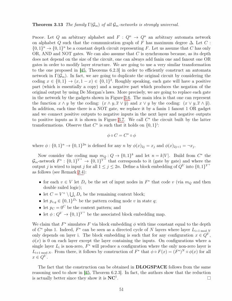
Theorem 3.13 The family �(Gm) of all Gm-networks is strongly universal.

Proof. Let Q an arbitrary alphabet and F : Qn ! Qn an arbitrary automata networkon alphabet Q such that the communication graph of F has maximum degree �. Let C :

{0, 1}n ! {0, 1}n be a constant depth circuit representing F . Let us assume that C has onlyOR, AND and NOT gates. We can also assume that C is synchronous because, as its depthdoes not depend on the size of the circuit, one can always add fanin one and fanout one ORgates in order to modify layer structure. We are going to use a very similar transformationto the one proposed in [45, Theorems 6.2.3] in order to efficiently construct an automatanetwork in �(Gm). In fact, we are going to duplicate the original circuit by considering thecoding x 2 {0, 1} ! (x, 1 � x) 2 {0, 1}2. Roughly speaking, each gate will have a positivepart (which is essentially a copy) and a negative part which produces the negation of theoriginal output by using De Morgan’s laws. More precisely, we are going to replace each gatein the network by the gadgets shown in Figure 3.6. The main idea is that one can representthe function x ^ y by the coding: (x ^ y, x _ y) and x _ y by the coding: (x _ y, x ^ y).In addition, each time there is a NOT gate, we replace it by a fanin 1 fanout 1 OR gadgetand we connect positive outputs to negative inputs in the next layer and negative outputsto positive inputs as it is shown in Figure 3.7. We call C⇤ the circuit built by the lattertransformations. Observe that C⇤ is such that it holds on {0, 1}i:

� � C = C⇤ � �

where � : {0, 1}n ! {0, 1}2n is defined for any n by �(x)2j = xj and �(x)2j+1 = ¬xj.

Now consider the coding map mQ : Q! {0, 1}k and let n = k|V |. Build from C⇤ theGm-network F ⇤

: {0, 1}V + ! {0, 1}V + that corresponds to it (gate by gate) and where theoutput j is wired to input j for all 1 j 2n. Define a block embedding of QV into {0, 1}V +

as follows (see Remark 2.4):

• for each v 2 V let Dv be the set of input nodes in F ⇤ that code v (via mQ and thendouble railed logic);

• let C = V + \S

v Dv be the remaining context block;• let pv,q 2 {0, 1}Dv be the pattern coding node v in state q;• let pC = 0

C be the context pattern; and• let � : QV ! {0, 1}V + be the associated block embedding map.

We claim that F ⇤ simulates F via block embedding � with time constant equal to the depthof C⇤ plus 1. Indeed, F ⇤ can be seen as a directed cycle of N layers where layer Li+1 mod N

only depends on layer i. The block embedding is such that for any configuration x 2 QV ,�(x) is 0 on each layer except the layer containing the inputs. On configurations where asingle layer Li is non-zero, F ⇤ will produce a configuration where the only non-zero layer isLi+1 mod N . From there, it follows by construction of F ⇤ that � � F (x) = (F ⇤

)N � �(x) for all

x 2 QV .

The fact that the construction can be obtained in DLOGSPACE follows from the samereasoning used to show in [45, Theorem 6.2.3]. In fact, the authors show that the reductionis actually better since they show it is NC

1.

51

^

x y

x ^ y x ^ y

_

x y

x _ y x _ y

x ^ yx ^ y

yx

^

x _ yx _ y

yx

_

x _ yx _ y

yx

_

x ^ yx ^ y

yx

^

Figure 3.6: AND and OR gadgets for simulating AND/OR gates with fanin and fanout 2.For other values of fanin and fanout gadgets are the same but considering different numberof inputs/outputs.

_

y

x _ y x _ y

x

_

y

x _ y x _ y

^

y

x ^ y x ^ y

_

x

x

_

x

¬

x

x

Figure 3.7: NOT gadget wiring for circuit simulation using gates from Gm. In this case aNOT gate is connected to an OR gate in the original circuit. Copies of the NOT gate in thecircuit performing simulation are connected to the copies of the OR gate switched: positivepart is connected to negative part of the OR gate and viceversa.

52

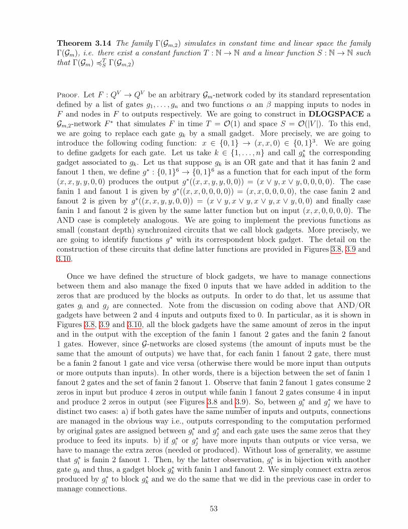
Theorem 3.14 The family �(Gm,2) simulates in constant time and linear space the family�(Gm), i.e. there exist a constant function T : N! N and a linear function S : N! N suchthat �(Gm) 4T

S �(Gm,2)

Proof. Let F : QV ! QV be an arbitrary Gm-network coded by its standard representationdefined by a list of gates g1, . . . , gn and two functions ↵ an � mapping inputs to nodes inF and nodes in F to outputs respectively. We are going to construct in DLOGSPACE aGm,2-network F ⇤ that simulates F in time T = O(1) and space S = O(|V |). To this end,we are going to replace each gate gk by a small gadget. More precisely, we are going tointroduce the following coding function: x 2 {0, 1} ! (x, x, 0) 2 {0, 1}3. We are goingto define gadgets for each gate. Let us take k 2 {1, . . . , n} and call g⇤k the correspondinggadget associated to gk. Let us that suppose gk is an OR gate and that it has fanin 2 andfanout 1 then, we define g⇤ : {0, 1}6 ! {0, 1}6 as a function that for each input of the form(x, x, y, y, 0, 0) produces the output g⇤((x, x, y, y, 0, 0)) = (x _ y, x _ y, 0, 0, 0, 0). The casefanin 1 and fanout 1 is given by g⇤((x, x, 0, 0, 0, 0)) = (x, x, 0, 0, 0, 0), the case fanin 2 andfanout 2 is given by g⇤((x, x, y, y, 0, 0)) = (x _ y, x _ y, x _ y, x _ y, 0, 0) and finally casefanin 1 and fanout 2 is given by the same latter function but on input (x, x, 0, 0, 0, 0). TheAND case is completely analogous. We are going to implement the previous functions assmall (constant depth) synchronized circuits that we call block gadgets. More precisely, weare going to identify functions g⇤ with its correspondent block gadget. The detail on theconstruction of these circuits that define latter functions are provided in Figures 3.8, 3.9 and3.10.

Once we have defined the structure of block gadgets, we have to manage connectionsbetween them and also manage the fixed 0 inputs that we have added in addition to thezeros that are produced by the blocks as outputs. In order to do that, let us assume thatgates gi and gj are connected. Note from the discussion on coding above that AND/ORgadgets have between 2 and 4 inputs and outputs fixed to 0. In particular, as it is shown inFigures 3.8, 3.9 and 3.10, all the block gadgets have the same amount of zeros in the inputand in the output with the exception of the fanin 1 fanout 2 gates and the fanin 2 fanout1 gates. However, since G-networks are closed systems (the amount of inputs must be thesame that the amount of outputs) we have that, for each fanin 1 fanout 2 gate, there mustbe a fanin 2 fanout 1 gate and vice versa (otherwise there would be more input than outputsor more outputs than inputs). In other words, there is a bijection between the set of fanin 1

fanout 2 gates and the set of fanin 2 fanout 1. Observe that fanin 2 fanout 1 gates consume 2

zeros in input but produce 4 zeros in output while fanin 1 fanout 2 gates consume 4 in inputand produce 2 zeros in output (see Figures 3.8 and 3.9). So, between g⇤

iand g⇤j we have to

distinct two cases: a) if both gates have the same number of inputs and outputs, connectionsare managed in the obvious way i.e., outputs corresponding to the computation performedby original gates are assigned between g⇤

iand g⇤j and each gate uses the same zeros that they

produce to feed its inputs. b) if g⇤i

or g⇤j have more inputs than outputs or vice versa, wehave to manage the extra zeros (needed or produced). Without loss of generality, we assumethat g⇤

iis fanin 2 fanout 1. Then, by the latter observation, g⇤

iis in bijection with another

gate gk and thus, a gadget block g⇤k with fanin 1 and fanout 2. We simply connect extra zerosproduced by g⇤

ito block g⇤k and we do the same that we did in the previous case in order to

manage connections.

53

Note that F ⇤ can be built in DLOGSPACE since it suffices to read the standard repre-sentation of F and produce associated block gadgets which have constant size. In additionwe have that previous encoding g ! g⇤ induces a block map � : {0, 1}V ! {0, 1}V + where|V +| = O(|V |) and that � � F = F ⇤T � � where T = 6 is the size of each gadget block in F ⇤.We conclude that F ⇤ 2 �(Gm,2) simulates F in space |V +| = O(|V |) and time T = 6 andthus, �(Gm) 4T

S �(Gm,2) where T is constant and S is a linear function.

Corollary 3.15 The family �(Gm,2) is strongly universal.

Proof. The result comes directly from Theorem 3.13 (�(Gm) is strongly universal) and The-orem 3.14 (�(Gm) 4T

S �(Gm,2) where T is constant and S is a linear function).

Now we show a result on universality of �(Gm) which is essentially a consequence of [45,Theorem 6.2.5]. The latter result starts with alternated monotonic circuit which has onlyfanin 2 and fanout 2 gates (previous results in the same reference show that one can alwaysreduce to this case starting from an arbitrary circuit) and gives an NC

1 construction of asynchronous alternating circuit preserving the previous property on the fanin and fanout ofeach gate. The main remark in this context is that the construction uses quadratic space inthe number of gates of the circuit given in input, so we cannot show strong universality butonly universality with this approach.

Theorem 3.16 The family �(Gm) of all Gm-networks is universal.

Proof. Let F : Qk ! Qk be some arbitrary network with a circuit representation C :

{0, 1}n ! {0, 1}n such that n = kO(1). By [45, Theorem 6.2.5] we can assume that thereexists a circuit C 0

: {0, 1}n0 ! {0, 1}n0 where n0= O(n2

) such that C 0 is synchronousalternated and monotonic. In addition, every gate in C 0 has fanin and fanout 2. We remarkthat the latter reference does not only provide the standard encoding of C 0 but also gives usa DLOGSPACE algorithm (it is actually NC

1) which takes the standard representation ofC : {0, 1}n ! {0, 1}n and produces C 0. We are going to slightly modify the latter algorithmin order to construct not only a circuit but a Gm-network. In fact, the only critical point is tomanage the identification between outputs and inputs. This is not direct from the result byRuzzo et al. as their algorithm involves duplication of inputs and also adding constant inputs.In order to manage this, it suffices to modify their construction in order to mark original,copies and constant inputs. Then, as Gm includes COPY gates and also AND/OR gateswith fanout 1, one can always produce copies of certain input if we need more, or erase extracopies of outputs or constants produced at output by adding a small circuit of O(log(n)) depthconsisting in a several fanin 2 fanout 1 gates forming a tree. Same idea applies for constantinputs. Formally, at the end of the algorithm, the DLOGSPACE algorithm can read extrainformation regarding copies and constant inputs, and then can construct a O(log(n)) depthcircuit that produces a coherent encoding for inputs and outputs. This latter constructiondefines a Gm-network G : {0, 1}n00 ! {0, 1}n00 and an encoding � : Qn ! {0, 1}n00 where

54

^ ^ _

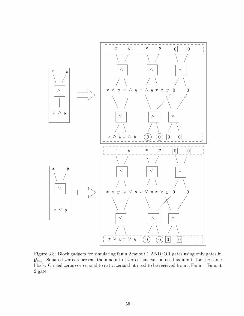
yx

x ^ y x ^ y

^ ^_

x ^ y x ^ y 0 0 0 0

yx

x ^ y x ^ y

0 0

0 0

x ^ y

yx

^

_ _ _

yx

x _ y x _ y

^ ^_

_

x y

x _ y

yx

x _ y x _ y

0 0

0 0

0000x _ yx _ y

Figure 3.8: Block gadgets for simulating fanin 2 fanout 1 AND/OR gates using only gates inGm,2. Squared zeros represent the amount of zeros that can be used as inputs for the sameblock. Circled zeros correspond to extra zeros that need to be received from a Fanin 1 Fanout2 gate.

55

_ _ _

0x

x x

_

_

x

x x

_ _

0x

x x

0 0

0 0

00xx x x

xx

x

^

_ _ _

0x

_

_

_ _

0x

x x

0 0

0 0

00xx

x

x

x

x

^

0 0

0 0

Figure 3.9: Block gadgets for simulating fanin 1 fanout 2 and fanin 1 fanout 1 AND/ORgates using only gates in Gm,2. Squared zeros represent the amount of zeros that can be usedas inputs for the same block. Circled zeros correspond to extra zeros that need to be receivedfrom a fanin 2 fanout 1 gate.

56

_ _ _

yx

x _ y x _ y

_ __

yx

x _ y x _ y

0 0

0 0

00x _ yx _ y

_

x _ y x _ y

yx

x _ y x _ y

_

yxyx

x ^ y

0 0

00x ^ yx ^ y

^

x ^ y x ^ y

yx

x ^ y x ^ y

^ ^

x ^ y x ^ y

^ _^

x ^ y 0 0

Figure 3.10: Block gadgets for simulating fanin 2 fanout 2 AND/OR gates using only gatesin Gm,2. Squared zeros represent the amount of zeros that can be used as inputs for the sameblock.

57

n00= O(n2

) such that � � F = GT � � where T = O(depth(C’) + log(n)). Thus, Gm isuniversal.

We present now the following direct corollary.

Corollary 3.17 Let F be a strongly universal automata network family. Then, F is univer-sal.

Proof. It suffices to exhibit a G-network family (G-networks are bounded degree networks)which is strongly universal and universal at the same time. By Theorem 3.16 we take G = Gm

and thus, the corollary holds.

Corollary 3.18 Let G be either Gm or Gm,2. Any family F that has coherent G-gadgetscontains a subfamily of bounded degree networks with bounded degree representation which is(strongly) universal. Any CSAN family with coherent G-gadgets is (strongly) universal.

3.3.1 Closure and synchronous closure

Although monotonic gates are sometimes easier to realize in concrete dynamical systems,which make the above results useful, there is nothing special about them to achieve uni-versality: any set of gates that are expressive enough for Boolean functions yields the sameuniversality result. Given a set of maps G over alphabet Q, we define its closure G as theset of maps that are computed by circuits that can be built using only gates from G. Moreprecisely, G is the closure of G by composition, i.e. forming from maps g1 : QI1 ! QO1 andg2 : QI2 ! QO2 (with I1, I2, O1, O2 disjoint) a composition g by plugging a subset of outputsO ✓ O2 of g1 into a subset of inputs I ✓ I2 of g2, thus obtaining g : QI1[I2\I ! QO1\O[O2

with

g(x)o =

(g1(xI1)o if o 2 O1 \O,

g2(y)o if o 2 O2,

where yj = xj for j 2 I2 \ I and yj = g1(xI1)⇡(j), where ⇡ : I ! O is the chosen bijectionbetween I and O (the wiring of outputs of g1 to inputs of g2). A composition is synchronousif either I = ; or I = I2. We then define the synchronous closure G2 as the closure bysynchronous composition. The synchronous composition correspond to synchronous circuitswith gates in G. A G-circuit is a sequence of compositions starting from elements of G. It issynchronous if the compositions are synchronous. The depth of a G-circuit is the maximallength of a path from an input to an output. In the case of a synchronous circuits, all suchpaths are of equal length.

Proposition 3.19 Fix some alphabet Q and consider two finite sets of maps G and G 0 overalphabet Q such that:

• either G contains the identity map Q! Q and is such that G contains G 0;

58

Figure 3.11: (Left panel) Non-synchronous composition and (Right panel) synchronous com-position.

• or there is an integer k such that G2

k, the set of elements of G2 that can be realized bya circuit of depth k contains G 0.

Then, any family F that has coherent G-gadgets has coherent G 0-gadgets.

Proof. Suppose first that the first item holds. Since G contains G 0 there must exist a circuitmade of gates from G that produces any given element g 2 G 0. Then one wants to applygadget glueing on gadgets from G to mimic the composition and thus obtain a gadget corre-sponding to g. However this does not work as simply because propagation delay is a priorinot respected at each gate in the circuit composition yielding g since layers in the circuitcould be connected in a way such that the information arrives at different times to eachlayer. However, since G contains the identity map, there is a corresponding gadget in thefamily that actually implements a delay line, allowing us to synchronize the evaluation ofthe circuit. This additional gadget solves the problem: it is straightforward to transform bypadding with identity gates all circuits with gates in G into synchronous ones. Moreover, bypadding again, we can assume that the finite set of such circuits computing elements of Gm

are all of same depth.Then, this set of circuits can be trasformed into coherent Gm-gadgetsby iterating gadget glueing and using Lemma 3.2.

If the second item holds the situation is actually simpler because the synchronous closurecontains only synchronous circuits of gates from Gm,2. So we can directly translate the circuitsproducing the maps of Gm,2 into gadgets via gadget glueing by Lemma 3.2 as in the previouscase. Moreover, as a consequence of the hypothesis, we have that each circuit in the set ofcircuits having gates in G 0 can be considered to have the same depth. Thus, we get gadgetsthat share the same time constant.

3.3.2 Super-polynomial periods without universality

A universal family must exhibit super-polynomial periods, however universality is far fromnecessary to have this dynamical feature. In this subsection we define the family of wirenetworks to illustrate this.

To this end, we need the following classical result about the growth of Chebyshev functionand prime number theorem.

59

Lemma 3.20 [47] Let m � 2 and P(m) = {p m | p prime}. If we define ⇡(m) = |P(m)|and ✓(m) =

Pp2P(m)

log(p) then we have ⇡(m) ⇠ mlog(m)

and ✓(m) ⇠ m.

By using the Lemma 3.20 we can construct automata networks with non-polynomial limitcycles simply by making disjoint union of rotations (i.e. network whose interaction graph is acycle graph that just rotate the configuration at each step). Indeed, it is sufficient to considerrotations on cycle graphs whose length are successive prime numbers. It turns out that theseautomata networks are exactly Gw-networks where Gw is a single ’wire gate’: Gw = {idB}where idB is the identity map over {0, 1}.

Formally, according to Definition 3.4 (see Figure 3.4), for any Gw-network F : QV ! QV

there exist a partition V = C1 [ C2 . . . [ Ck where Ci = {ui

1. . . , ui

li} with li � 2 for each

i = 1, . . . , k and F (x)uis+1 mod li

= xuis

for any x 2 QV and 0 s li.

Theorem 3.21 Any family F that has coherent Gw-gadgets has superpolynomial limit cycles,more precisely: there is some ↵ > 0 such that for infinitely many n 2 N, there exists a networkFn 2 F with O(n) nodes and a periodic orbit of size ⌦(exp(n↵

)).

Proof. Taking the notations of Lemma 3.20, define for any n the Gw-network Gn made ofdisjoint union of cycle graphs of each prime length less than n. Gn has size at most n⇡(n)and if we consider a configuration x which is in state 1 at exactly one node in each of the ⇡(n)disjoint cycle graphs, it is clear that the orbit of x is periodic of period exp ✓(n). Therefore,from Lemma 3.20, for any n, Gn is a cycle graph of size m n⇡(n) with a periodic orbit ofsize ✓(n) 2 ⌦(exp(

pm logm)). By hypothesis there are linear maps T and S such that for any

n, there is Fn that simulates Gn (by Lemma 3.10), therefore Fn also has a super-polynomiallimit cycle cycle by Lemma 2.6.

3.3.3 Conjunctive networks and Gconj-networks

Let G = (V,E) be any directed graph. The conjunctive network associated to G is the au-tomata network FG : {0, 1}V ! {0, 1}V given by F (x)i = ^j2N�(i)xj where N�

(i) denotesthe incoming neighborhood of i. Conjunctive networks are thus completely determinedby the interaction graph and a circuit representation can be deduced from this graph inDLOGSPACE. We define the family Fconj as the set of conjunctive networks together withthe standard representation F⇤

conj which are just directed graphs encoded as finite words ina canonical way.

Remark 3.22 We can of course do the same with disjunctive networks. Any conjunctivenetwork FG on graph G is conjugated to the disjunctive network F 0

G on the same graph bythe negation map ⇢ : {0, 1}V ! {0, 1}V defined by ⇢(x)i = 1� xi, formally ⇢ � FG = F 0

G � ⇢.In particular, this means that the families of conjunctive and disjunctive networks simulateeach other. In the sequel we will only state results for conjunctive networks while they holdfor disjunctive networks as well.

60

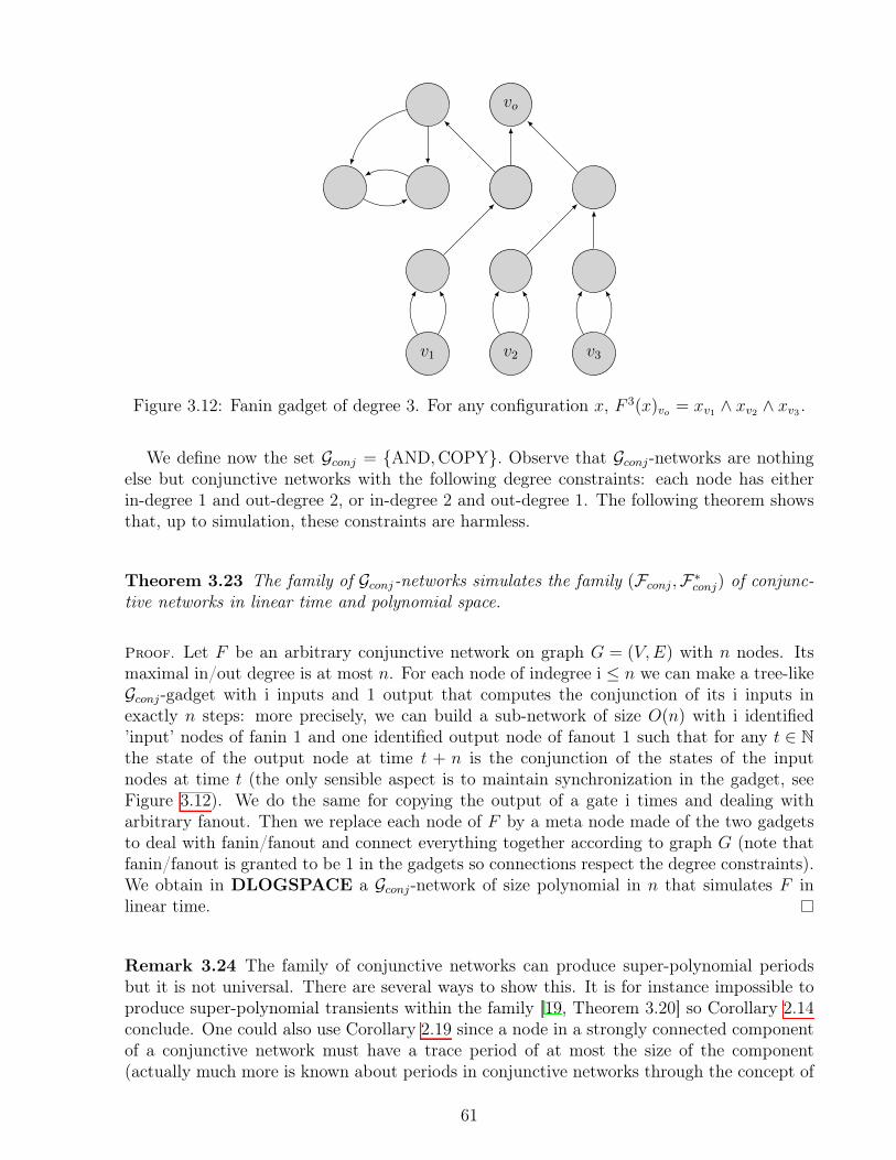
v1 v2 v3

vo

Figure 3.12: Fanin gadget of degree 3. For any configuration x, F 3(x)vo = xv1 ^ xv2 ^ xv3 .

We define now the set Gconj = {AND,COPY}. Observe that Gconj-networks are nothingelse but conjunctive networks with the following degree constraints: each node has eitherin-degree 1 and out-degree 2, or in-degree 2 and out-degree 1. The following theorem showsthat, up to simulation, these constraints are harmless.

Theorem 3.23 The family of Gconj-networks simulates the family (Fconj,F⇤conj) of conjunc-

tive networks in linear time and polynomial space.

Proof. Let F be an arbitrary conjunctive network on graph G = (V,E) with n nodes. Itsmaximal in/out degree is at most n. For each node of indegree i n we can make a tree-likeGconj-gadget with i inputs and 1 output that computes the conjunction of its i inputs inexactly n steps: more precisely, we can build a sub-network of size O(n) with i identified’input’ nodes of fanin 1 and one identified output node of fanout 1 such that for any t 2 Nthe state of the output node at time t + n is the conjunction of the states of the inputnodes at time t (the only sensible aspect is to maintain synchronization in the gadget, seeFigure 3.12). We do the same for copying the output of a gate i times and dealing witharbitrary fanout. Then we replace each node of F by a meta node made of the two gadgetsto deal with fanin/fanout and connect everything together according to graph G (note thatfanin/fanout is granted to be 1 in the gadgets so connections respect the degree constraints).We obtain in DLOGSPACE a Gconj-network of size polynomial in n that simulates F inlinear time.

Remark 3.24 The family of conjunctive networks can produce super-polynomial periodsbut it is not universal. There are several ways to show this. It is for instance impossible toproduce super-polynomial transients within the family [19, Theorem 3.20] so Corollary 2.14conclude. One could also use Corollary 2.19 since a node in a strongly connected componentof a conjunctive network must have a trace period of at most the size of the component(actually much more is known about periods in conjunctive networks through the concept of

61

loop number or cyclicity, see [19]).

3.3.4 Super-polynomial transients without universality

Let us consider in this section the alphabet Q = {0, 1, 2}. We are going to define a set Gt

such that Gt-networks exhibit super-polynomial transients but are not universal. To helpintuition, Gt-networks can be though as standard conjunctive networks on {0, 1} that can insome circumstances produce state 2 which is a spreading state (a node switches to state 2

if one of its incoming neighbors is in state 2). The extra state 2 will serve to mark super-polynomial transients, but it cannot escape a strongly connected component once it appearsin it. As we will see, Gt-networks are therefore too limited in their ability to produce largeperiodic behavior inside strongly connected components.

Gt is made of the following maps:

AND{0,1} : (x, y) 7!(2 if 2 2 {x, y}x ^ y else.

AND2 : (x, y) 7!(2 if 2 2 {x, y} or x = y = 1

0 else.

⇤ : (x, y) 7!(2 if 2 2 {x, y}x else.

Id : x 7! x.

⌥ : x 7! (x, x).

Gt-networks can produce non-polynomial cycles by disjoint union of rotations of primelengths as in Theorem 3.21, but they can also wait for a global synchronization of all rotationsand freeze the result of the test for this synchronization condition inside a small feedbackloop attached to a “controlled AND map”.

More precisely, as shown in Figure 3.13 we can use in the context of any Gt-network a smallmodule T (x) made of five nodes with the following property: if the ⇤ node of the module isin state 0 in some initial configuration, then it stays in state 0 as long as node x is not instate 1, and when x = 1 at some time step t then, from step t + 2, the ⇤ node is in state 2

at least one step every two steps. This module is the key to control transient behavior.

Moreover, map AND{0,1} behaves like standard Boolean AND map when its inputs are in{0, 1}. More generally, by combining such maps in a tree-like fashion, one can build modulesA(x1, . . . , xk) for any number k of inputs with a special output node which has the followingproperty for some time delay � 2 O(log(k)): the output node at time t+� is in state 1 ifand only if all nodes xi (with 1 i k) are in state 1 at time t.

Combining these two ingredients, we can build upon the construction of Theorem 3.21 toobtain non-polynomial transients in any family having coherent Gt-gadgets.

Theorem 3.25 Any family F that has coherent Gt-gadgets has superpolynomial transients,

62

AND2⌥1

⌥2

⇤

x Id

Figure 3.13: Freezing the result of a test in a Gt-network. The module T (x) is made of thenodes marked ⌥, AND2, ⇤ and Id. Observe that each node represent some output of itscorresponding label(for more details on G-networks see Definition 3.4). Each gate has oneoutput with the exception of the gate ⌥ which is represented by two nodes. The moduleT (x) reads the value of node x belonging to an arbitrary Gt-network (represented in light grayinside dotted lines). The output ⇤ is fed back to its control input via the Id node (self-loopsare forbidden in Gt-networks). Note that x as well as the rest of the network is not influencedby the behavior of the gates of the module T (x).

more precisely: there is some ↵ > 0 such that for any n 2 N, there exists a network Fn 2 Fwith O(n) nodes and a configuration x such that F t

n(x) is not in an attractor of Fn witht 2 ⌦(exp(n↵

)).

Proof. Like in Theorem 3.21, they key of the proof is to show that there is a Gt-networkwith transient length as in the theorem statement, then the property immediately holds fornetworks of the family F by Lemma 3.10 and Lemma 2.6.

For any n > 0 we construct a Gt-network Gn made of two parts:

• The “bottom” part of Gn uses a polynomial set of nodes Bn and consists in a disjointunion of circuits for each prime length less than n as in Theorem 3.21, but where foreach prime p, the circuit of length p has a node vp which implements a copy gate COPY,thus not only sending its value to the next node in the circuit, but also outputting itto the “top” part of Gn.

• The “top” part of Gn is made of a module A(x1, . . . , xk) connected to all nodes vp asinputs and whose output is connected to a test module T (x) as in Figure 3.13.

Note that the size of Gn is polynomial in n. With this construction we have the followingproperty as soon as the modules A(x1, . . . , xk) and T (x) are initialized to state 0 everywhere:as long as nodes vp are not simultaneously in state 1 then the output of the test moduleT (x) stays in state 0; moreover, if at some time t nodes vp are simultaneously in state t, thenafter time t + O(log(t)), the node ⇤ of module T (x) is in state 2 one step every two steps.This means that t + O(log(t)) is a lower bound on the transient of the considered orbit. Toconclude the proof it is sufficient to consider the initial configuration where all nodes are instate 0 except the successor of node vp in each circuit of prime length p, which are in state 1.In this case it is clear that the first time t at which all nodes vp are in state 1 is the productof prime numbers less than n. As in Theorem 3.21, we conclude thanks to Lemma 3.20.

As said above, Gt-networks are limited in their ability to produce large periods. More

63

precisely, as shown by the following lemma, their behavior is close enough to conjunctivenetworks so that it can be analyzed as the superposition of the propagation/creation of state2 above the behavior of a classical Boolean conjunctive network. To any Gt-network F weassociate the Boolean conjunctive network F ⇤ with alphabet {0, 1} as follows: nodes withlocal map AND{0,1} or AND2 are simply transformed into nodes with Boolean conjunctivelocal maps on the same neighbors, nodes with local maps ⌥ or Id are left unchanged (onlytheir alphabet changes), and nodes with map ⇤(x, y) are transformed into a node with onlyx as incoming neighborhood.

Lemma 3.26 Let F be a Gt-network with node set V and F ⇤ its associated Boolean con-junctive network. Consider any x 2 {0, 1, 2}V and any x⇤ 2 {0, 1}V such that the followingholds:

8v 2 V : xv 2 {0, 1}) x⇤v = xv,

then the same holds after one step of each network:

8v 2 V : F (x)v 2 {0, 1}) F ⇤(x⇤

)v = F (x)v.

Proof. It is sufficient to check that if F (x)v 6= 2, it means that all its incoming neighborsare in {0, 1} so x and x⇤ are equal on these incoming neighbors, and that it only depends onneighbor a in the case of a local map ⇤(a, b). In any case, we deduce F ⇤

(x⇤)v = F (x)v by

definition of F ⇤.

Theorem 3.27 The family of Gt-networks is not universal.

Proof. Consider a Boolean conjunctive automata network F , a configuration x with periodicorbit under F and some node v such that there is a walk of length L from v to v. We claimthat xv = FL

(x)v so the trace at node v in x is periodic of period less than L. Indeed,in a conjunctive network state 0 is spreading so clearly if xv = 0 then FL

(x)v = 0 and,more generally, F kL

(x)v = 0 for any k � 1. On the contrary, if xv = 1 then we cannot haveFL

(x)v = 0 because then F Pk(x)v = 0 with P the period of x which would imply xv = 0.

With the same reasoning, if we consider any Gt-network F , any configuration x withperiodic orbit and some node v such that there is a walk of length L from v to v, then itholds:

xv = 2, FL(x)v = 2.

We deduce thanks to Lemma 3.26 that for any configuration x with periodic orbit of some Gt-network F with n nodes, and for any node v belonging to some strongly connected component,the period of the trace at v starting from x is less than n2: it is a periodic pattern of presenceof state 2 of length less than n superposed on a periodic trace on {0, 1} of length less than n.We conclude that the family of Gt-networks cannot be universal thanks to Theorem 2.19.

64

Chapter 4

Describing asynchronous dynamics: adeterministic approach

In this chapter, we study the dynamics of automata networks under different update schemes.Recall that, generally speaking, automata networks dynamics is defined in terms of a globalrule F : Qn ! Qn. If we see now F as a network, i.e. a collection of entities that are somehowrelated, we can interpret the evolution of this dynamics as defined by a scheme in whicheach of these entities is updated at the same time. This dynamics is usually called parallelor synchronous. As we have pointed out previously, this approach is considered usuallyunrealistic for some applications. Probably the most iconic case (to consider) in this contextis that of applications in gene regulatory networks. Within this domain, the synchronousdynamics seems to be inaccurate since it can be interpreted as a type of dynamics in whichthe expression of all genes takes place simultaneously. Considering the latter observation,there are some classical types of breaking the synchronous update scheme or introducingasynchronicity to the dynamics of a fixed automata network. As we work mainly withCSAN families for all the applications considered in Chapter 5, we define update schemesexclusively for this type of automata networks. However, all our definitions can be extendedto the general case. Particularly, we explore in the first section of this chapter three classes ofupdate schemes which are widely referenced in the literature and also studied from the pointof view of how they impact the original synchronous dynamics. These classes are: periodicupdate schemes, local clocks update schemes and block sequential update schemes. We startby establishing a strict hierarchy between these three classes and studying some examples.We discuss also the limits of periodic dynamics compared to other types of update schemes.Then, we present a general framework which allows us to see the dynamics defined by meansof update schemes as a projection of the dynamics of another automata network which isdeterministic and operates over a bigger alphabet, which contains the original alphabet as acomponent. This approach does not only include periodic update schemes, and thus, localclocks and block sequential update schemes, but also considers some of more general updateschemes that we will define in this section.

65

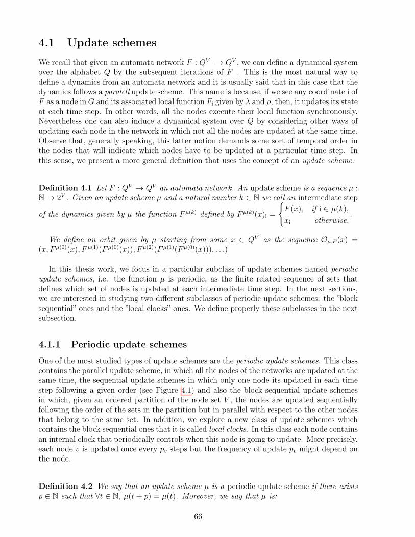
4.1 Update schemesWe recall that given an automata network F : QV ! QV , we can define a dynamical systemover the alphabet Q by the subsequent iterations of F . This is the most natural way todefine a dynamics from an automata network and it is usually said that in this case that thedynamics follows a paralell update scheme. This name is because, if we see any coordinate i ofF as a node in G and its associated local function Fi given by � and ⇢, then, it updates its stateat each time step. In other words, all the nodes execute their local function synchronously.Nevertheless one can also induce a dynamical system over Q by considering other ways ofupdating each node in the network in which not all the nodes are updated at the same time.Observe that, generally speaking, this latter notion demands some sort of temporal order inthe nodes that will indicate which nodes have to be updated at a particular time step. Inthis sense, we present a more general definition that uses the concept of an update scheme.

Definition 4.1 Let F : QV ! QV an automata network. An update scheme is a sequence µ :

N! 2V . Given an update scheme µ and a natural number k 2 N we call an intermediate step

of the dynamics given by µ the function F µ(k) defined by F µ(k)(x)i =

(F (x)i if i 2 µ(k),

xi otherwise..

We define an orbit given by µ starting from some x 2 QV as the sequence Oµ,F (x) =

(x, F µ(0)(x), F µ(1)

(F µ(0)(x)), F µ(2)

(F µ(1)(F µ(0)

(x))), . . .)

In this thesis work, we focus in a particular subclass of update schemes named periodicupdate schemes, i.e. the function µ is periodic, as the finite related sequence of sets thatdefines which set of nodes is updated at each intermediate time step. In the next sections,we are interested in studying two different subclasses of periodic update schemes: the ”blocksequential” ones and the ”local clocks” ones. We define properly these subclasses in the nextsubsection.

4.1.1 Periodic update schemes

One of the most studied types of update schemes are the periodic update schemes. This classcontains the parallel update scheme, in which all the nodes of the networks are updated at thesame time, the sequential update schemes in which only one node its updated in each timestep following a given order (see Figure 4.1) and also the block sequential update schemesin which, given an ordered partition of the node set V , the nodes are updated sequentiallyfollowing the order of the sets in the partition but in parallel with respect to the other nodesthat belong to the same set. In addition, we explore a new class of update schemes whichcontains the block sequential ones that it is called local clocks. In this class each node containsan internal clock that periodically controls when this node is going to update. More precisely,each node v is updated once every pv steps but the frequency of update pv might depend onthe node.

Definition 4.2 We say that an update scheme µ is a periodic update scheme if there existsp 2 N such that 8t 2 N, µ(t+ p) = µ(t). Moreover, we say that µ is:

66

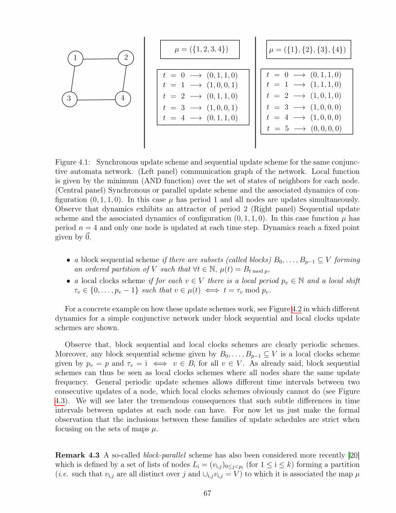
t = 0 �! (0, 1, 1, 0)t = 1 �! (1, 0, 0, 1)

t = 2 �! (0, 1, 1, 0)

t = 3 �! (1, 0, 0, 1)t = 4 �! (0, 1, 1, 0)

µ = ({1, 2, 3, 4})1 2

43

t = 5 �! (0, 0, 0, 0)

µ = ({1}, {2}, {3}, {4})

t = 4 �! (1, 0, 0, 0)t = 3 �! (1, 0, 0, 0)

t = 2 �! (1, 0, 1, 0)

t = 1 �! (1, 1, 1, 0)t = 0 �! (0, 1, 1, 0)

Figure 4.1: Synchronous update scheme and sequential update scheme for the same conjunc-tive automata network. (Left panel) communication graph of the network. Local functionis given by the minimum (AND function) over the set of states of neighbors for each node.(Central panel) Synchronous or parallel update scheme and the associated dynamics of con-figuration (0, 1, 1, 0). In this case µ has period 1 and all nodes are updates simultaneously.Observe that dynamics exhibits an attractor of period 2 (Right panel) Sequential updatescheme and the associated dynamics of configuration (0, 1, 1, 0). In this case function µ hasperiod n = 4 and only one node is updated at each time step. Dynamics reach a fixed pointgiven by ~0.

• a block sequential scheme if there are subsets (called blocks) B0, . . . , Bp�1 ✓ V formingan ordered partition of V such that 8t 2 N, µ(t) = Bt mod p,

• a local clocks scheme if for each v 2 V there is a local period pv 2 N and a local shift⌧v 2 {0, . . . , pv � 1} such that v 2 µ(t) () t = ⌧v mod pv.

For a concrete example on how these update schemes work, see Figure 4.2 in which differentdynamics for a simple conjunctive network under block sequential and local clocks updateschemes are shown.

Observe that, block sequential and local clocks schemes are clearly periodic schemes.Moreover, any block sequential scheme given by B0, . . . , Bp�1 ✓ V is a local clocks schemegiven by pv = p and ⌧v = i () v 2 Bi for all v 2 V . As already said, block sequentialschemes can thus be seen as local clocks schemes where all nodes share the same updatefrequency. General periodic update schemes allows different time intervals between twoconsecutive updates of a node, which local clocks schemes obviously cannot do (see Figure4.3). We will see later the tremendous consequences that such subtle differences in timeintervals between updates at each node can have. For now let us just make the formalobservation that the inclusions between these families of update schedules are strict whenfocusing on the sets of maps µ.

Remark 4.3 A so-called block-parallel scheme has also been considered more recently [20]which is defined by a set of lists of nodes Li = (vi,j)0j<pi (for 1 i k) forming a partition(i.e. such that vi,j are all distinct over j and [i,jvi,j = V ) to which it is associated the map µ

67

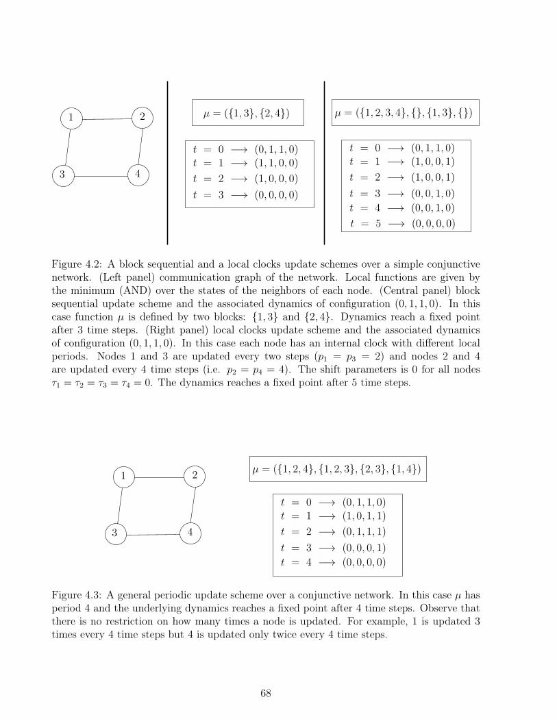
1 2

43

t = 0 �! (0, 1, 1, 0)t = 1 �! (1, 1, 0, 0)

t = 2 �! (1, 0, 0, 0)

t = 3 �! (0, 0, 0, 0)

µ = ({1, 3}, {2, 4})

t = 0 �! (0, 1, 1, 0)t = 1 �! (1, 0, 0, 1)

t = 2 �! (1, 0, 0, 1)

t = 3 �! (0, 0, 1, 0)t = 4 �! (0, 0, 1, 0)

µ = ({1, 2, 3, 4}, {}, {1, 3}, {})

t = 5 �! (0, 0, 0, 0)

Figure 4.2: A block sequential and a local clocks update schemes over a simple conjunctivenetwork. (Left panel) communication graph of the network. Local functions are given bythe minimum (AND) over the states of the neighbors of each node. (Central panel) blocksequential update scheme and the associated dynamics of configuration (0, 1, 1, 0). In thiscase function µ is defined by two blocks: {1, 3} and {2, 4}. Dynamics reach a fixed pointafter 3 time steps. (Right panel) local clocks update scheme and the associated dynamicsof configuration (0, 1, 1, 0). In this case each node has an internal clock with different localperiods. Nodes 1 and 3 are updated every two steps (p1 = p3 = 2) and nodes 2 and 4

are updated every 4 time steps (i.e. p2 = p4 = 4). The shift parameters is 0 for all nodes⌧1 = ⌧2 = ⌧3 = ⌧4 = 0. The dynamics reaches a fixed point after 5 time steps.

1 2

43

t = 0 �! (0, 1, 1, 0)t = 1 �! (1, 0, 1, 1)

t = 2 �! (0, 1, 1, 1)

t = 3 �! (0, 0, 0, 1)t = 4 �! (0, 0, 0, 0)

µ = ({1, 2, 4}, {1, 2, 3}, {2, 3}, {1, 4})

Figure 4.3: A general periodic update scheme over a conjunctive network. In this case µ hasperiod 4 and the underlying dynamics reaches a fixed point after 4 time steps. Observe thatthere is no restriction on how many times a node is updated. For example, 1 is updated 3

times every 4 time steps but 4 is updated only twice every 4 time steps.

68

1 2

43

t = 0 �! (0, 1, 1, 0)t = 1 �! (1, 0, 1, 1)

t = 2 �! (0, 0, 1, 0)

t = 3 �! (0, 0, 0, 0)

µ = ({1, 2, 4}, {1, 3, 4})

Figure 4.4: A block parallel update scheme defined over a conjunctive network. Updatinglist is given by L = {(1), (2, 3), (4)}. Observe that a constant amount of nodes (equal to thelength of L, i.e., 3) is updated at each time step. Dynamics reaches a fixed point after 3

time-steps.

such that vi,j 2 µ(n) () j = n mod pi. It is a particular case of our definition of local clocksscheme above with the additional constraints that the size of the set µ(n) of updated nodesis constant with n (see Figure 4.4 for an example). We note that, conversely, any local clocksscheme on a given network can be simulated by a block-parallel scheme by artificially addingdisconnected nodes that do nothing but satisfy the constraint of µ(n) being of constant size.

4.1.2 Projection systems

We recall that Q is a finite set that we call alphabet. Now we present a dynamical formalismthat allows us to include all the update schemes presented above and possibly other ones intoone formalism. We remark that in all periodic schemes, a given node can take the decisionto update or not by simply keeping track of the current value of time modulo the period.Thus, one could see the system as a non-deterministic system in which possibilities are givenby all the possible ways to update nodes respecting a periodic update scheme. However,a key observation in this context is that, when we add the knowledge of time modulo theperiod at each node as a new component of states, the whole system becomes deterministic.In fact, we can recover the original dynamics of some automata network with alphabet Qunder a periodic update scheme by projecting a specific deterministic automata network withalphabet Q0 ⇥Q onto Q.

Let F : QV ! QV be an automata network. We recall that its asynchronous versionis an automata network that at every time-step (non-deterministically) choose if a node i

should be updated or if it will be stay in the same state. More precisely, a asynchronousversion of F is a non-deterministic function F ⇤

: QV ! P(QV) such that F ⇤

(x) = {y 2QV

: 9U ⇢ V, yv = F (x)v if v 2 U and yv = xv otherwise.}. Equivalently, we can see F ⇤ asa function F ⇤

: QV ! (P(Q))V such that F ⇤

(x)i = {xi, F (x)i}. Note that, analogously tothe deterministic case one can define an orbit starting from x of F ⇤ as a sequence of statesOF ⇤(x) = x0

= x, x1, x2, . . . , xt, . . . ,2 Qn such that xsi2 F (xs�1

)i for i 2 V and s � 1. Notealso that, given x 2 QV and an orbit OF ⇤(x) we can see OF ⇤(x) as a particular realization ofa certain update scheme µ. More precisely, there exists an update scheme µ (which is definedin the obvious way i.e. by updating the corresponding nodes in every time step accordingto points in OF ⇤(x)) such that for every xs 2 OF ⇤(x) we have xs

= (OF,µ(x))s. In addition,

69

we have that for each update scheme µ there exist an orbit of F ⇤ which coincides with itsdynamics in every time step. Thus, we want to work with F ⇤ in order to globally study awhole class of update schemes. However, we would like to continue working in a deterministicframework in order to keep things simple (in particular the notion of simulation that wedefine later). In order to achieve this task, we introduce the following notion of asynchronousextension which is a way to produce the dynamics of different update schemes throughprojection.

Definition 4.4 Let Q be a finite alphabet and Q0= Q⇥R where R is finite. Let F : QV ! QV

and F 0: Q0V ! Q0V two automata networks. We say that F is a projection system of F’ and

that F’ is an asynchronous extension of F if:

8x 2 Q0V , ⇡(F 0(x)) 2 F ⇤

(⇡(x)), (4.1)

where ⇡ is the node-wise extension of the projection ⇡ : Q0 ! Q such that ⇡(q, r) = q for allq0 = (q, r) 2 Q0.

We show hereunder that the dynamics associated to any of the previously presented peri-odic update schemes can be described as an asynchronous extension over a product alphabet.To simplify notations we sometimes identify (A⇥ B ⇥ · · · )V with AV ⇥ BV ⇥ · · ·.

First we introduce the block sequential extensions. Generally speaking, given an orderedpartition {B1, . . . Bb} defining a block sequential update scheme, we define a product spacein which the second coordinate contains an internal clock which counts the evolution of timemodulo b. For each node, its corresponding block is coded in the initial configuration and itis updated every b time steps.

Definition 4.5 (block sequential extension) Let F : QV ! QV be an automata network. Letb n and let Q0

= Q⇥ {0, . . . , b� 1}. We define the block sequential extension of F with bblocks as the automata network F 0

: (Q0)V ! (Q0

)V such that for all x = (xQ, xb) 2 Q0V and

all v 2 V :

F 0(x)v =

((F (xQ)v, (xb)v � 1 mod b) if (xb)v = 0,

((xQ)v, (xb)v � 1 mod b) otherwise.

Now we introduce the definition of the local clocks extensions. In this case, as same as thecase of block sequential extensions, the second coordinate stores the dynamics of an internalclock which periodically registers the evolution of time. However, in local clocks updatescheme, each node can have its own local period, so clocks are note synchronized as in blocksequential extension. As a consequence, we have to define a third coordinate which containsthe information about the local period of each node. This component is constant and eachlocal period is bounded by some parameter c called clock delay.

Definition 4.6 (local clocks extension) Let F : QV ! QV be an automata network. Letc 2 N and let Q0

= Q ⇥ {0, . . . , c � 1} ⇥ {1, . . . , c}. We define the local clocks extensionof F with clock delay c as the automata network F 0

: (Q0)V ! (Q0

)V such that for all x =

70

(xQ, xc, xm) 2 Q0V and all v 2 V :

F 0(x)v =

((F (xQ)v, ( (xm)v

[(xc)v]) + 1 mod (xm)v, (xm)v) if (xc)v = 0,

((xQ)v, ( (xm)v[(xc)v]) + 1 mod (xm)v, (xm)v) else.

m(r) : {0, . . . , c� 1}! {0, . . . , c� 1} is such that m(r) =

(r if r m� 1,

m� 1 otherwise.

Observe that the function m cleans in one step any initially condition that is not coherentfor the local clock scheme (for example if some node starts with an initial value in its secondcoordinate that is greater than its local period). Finally, we present the periodic extension.The main difference between the latter definitions is that updates can be defined arbitrarilyover a fixed time interval which is defined through a period parameter p. In addition, wesay it is periodic because what happens in this time window must be repeated every p timessteps. Thus, we consider an internal clock coordinate (as same as the previous cases) togetherwith a third constant coordinate which serves as a marker for the set of time steps (over eachp steps time interval) in which each node is updated.

Definition 4.7 (periodic extension) Let F : QV ! QV be an automata network. Let p 2 Nand let Q0

= Q⇥{0, . . . , p�1}⇥2{0,...,p�1}. We define the periodic extension of F with period

length p as the automata network F 0: (Q0

)V ! (Q0

)V such that for all x = (xQ, xp, xs) 2 Q0V

and all v 2 V :

F 0(x)v =

((F (xQ)v, (xp)v + 1 mod p, (xs)v) if (xp)v 2 (xs)v,

((xQ)v, (xp)v + 1 mod p, (xs)v) otherwise.

This approach by asynchronous extensions can also capture non-periodic update schemes.For instance, an update scheme for Boolean networks called firing memory has been recentlystudied [32, 39, 67]. This update scheme, uses internal clocks at each node and, in addition,it makes the delay mechanism given by these clocks depend on the state of each node inthe current configuration. Roughly speaking, each node is updated at the same time but ithas an internal clock which works in a similar way as local clocks update scheme, with theexception that, this clock depends on the current state of each node in the following way: ifcertain node is in state 0 it will update its state following the original local rule (in fact, nodesin state 0 are forced to have their internal clocks in 0). Complementarily, if a node is in state1 and it is intended to change its state to 0 (for example in a conjunctive network this mayhappen if some other neighbor is in state 0) it will verify its internal clock. If its clock hasnot reach 0 then, it continues to the next value (it decreases its value) and its current statevalue is not updated (it remains in state 1). However, in any case (if node is in state 1 or instate 0), if node is intended to change its state to 1 then, its internal clock is restored to itsmaximum value independently of its current value (see Figure 4.5 for a concrete example).

Formally, given a boolean network F : {0, 1}n 7! {0, 1}n it is possible to define a new statespace by associating to each coordinate i of a configuration x 2 {0, 1}n an internal clock,given by some integer yi 2 {0, . . . , ⌧i} for some integers ⌧ = (⌧1, . . . , ⌧n) such that ⌧i � 1. In

71

this product space, we will define the following dynamics: First, for each (xi, yi), we compute,by using the original rule, the amount x0

i= F (x)i. Thus, the state (xi, yi) will be updated to

(x⇤i, y⇤

i) according to the following rules:

x⇤i=

(x

0

iif yi < 2,

1 if yi � 2,

and,

y⇤i=

8><

>:

0 if x0

i= 0 ^ yi < 2,

yi � 1 if x0

i= 0 ^ yi � 2,

⌧i. if x0

i= 1.

Firing memory schemes can be captured as an asynchronous extension in such a way thatthe resulting asynchronous extension is also a CSAN (see Lemma 4.9). We give hereunderthe precise definition of a firing memory extension:

Definition 4.8 (Firing memory extension) Let Q = {0, 1} and let F : QV ! QV be anautomata network. Let ⌧ 2 N and let Q0

= Q ⇥ {0, . . . , ⌧} ⇥ {0, . . . , ⌧}. We define a firingmemory extension of F with maximum delay ⌧ as the automata network F 0

: (Q0)V ! (Q0

)V

such that for all x = (xQ, x⌧ , xm) 2 Q0n we have that

F 0(x)v =

8>>><

>>>:

(1, (xm)v, (xm)v) if (x⌧ )v > 1 ^ fv(xQ|N(v)) = 1,

(1, ( (xm)v[(xc)v])� 1, (xm)v) if (x⌧ )v > 1 ^ fv(xQ|N(v)) = 0,

(1, (xm)v, (xm)v) if (x⌧ )v 1 ^ fv(xQ|N(i)) = 1,

(0,max{( (xm)v[(xc)v])� 1, 0}, (xm)v) if (x⌧ )v 1 ^ fv(xQ|N(v)) = 0,

where fv : QN(v) ! Q is such that F 0v ⌘ fv and m(r) : {0, . . . , ⌧} ! {0, . . . , ⌧} is such that

m[r] =

(r r m� 1

m� 1 otherwise

The previous definitions are formalized for every automata network. We now focus onCSAN families where the extensions are also CSAN as show in the following lemma.

Lemma 4.9 Let F be a CSAN, then any block sequential extension (resp. local clocks exten-sion, resp. periodic extension, resp. firing memory extension) of F is a CSAN. Moreover,for any CSAN family F and any fixed b (resp. c, resp. p, resp ⌧), the set of block sequentialextensions (resp. local clock extensions, resp. periodic, resp. firing memory extenstions) withb blocks (resp. with clock delay c, resp. with period p, resp. with maximum delay) of networksof F is again a CSAN family.

Proof. Observe first that for block sequential extensions (resp. local clocks extension, resp.periodic extension, resp. firing memory extension) the definition of F 0 considers an alphabetQ0

= Q ⇥ R such that the action of F 0 on the R component is purely local (the new valueof the R component of a node evolves as a function of the old value of this R component)

72

1 2

43

t = 0 �! (0, 1, 2, 3)t = 1 �! (3, 0, 1, 2)

t = 2 �! (2, 3, 0, 1)

t = 3 �! (1, 2, 3, 0)

t = 4 �! (0, 1, 2, 3)

Figure 4.5: A firing memory update scheme over a conjunctive network. Each local function isgiven by the minimum over the states of neighbors. The delay component (second componentin Definition 4.8) only is shown. Maximum delay of the network is ⌧ = 4. Dynamics describesan attractor of period 4 in which 0 circulates over the different nodes of the network. Notethat at any time, there is exactly one node in state 0, the other being in state 1 with differentdelay values.

and the value of the R component at a node determines alone if the Q component should beupdated according to F or left unchanged. Therefore clearly F 0 is a CSAN if F is.

In the context of a CSAN family F , the CSAN definition of F 0 involves only local con-straints coming from F 2 F and the action on the R-component is the same at each node.So the second part of the lemma is clear.

To sum up, our formalism allows to treat variations in the update scheme as a change inthe CSAN family considered. Given a CSAN family F and integers b, c, p, ⌧ , we introducethe following notations:

• Fblock,b is the CSAN family of all block sequential extensions of networks from F withb blocks,

• Fclock,c is the CSAN family of all local clocks sequential extensions of networks fromF with clock delay c,

• Fper,p is the CSAN family of all periodic extensions of networks from F with period p.• Ffir,⌧ is the CSAN family of all firing memory extensions of networks from F with

maximum delay ⌧ .

73

Chapter 5

Concrete symmetric automata networks:a case study

In this chapter, we focus on studying concrete symmetric automata network (CSAN) fam-ilies. We use previous theoretical framework on complexity of automata networks familiesin order to classify different CSAN families according to their dynamical behavior under dif-ferent update schemes. More precisely, we focus on two different families of CSAN: signedconjunctive networks and min-max networks. We distinguish three main subfamilies insidesigned conjunctive networks:

• symmetric conjunctive networks, which are regular conjunctive networks (in which alledge labels are the identity function);

• locally positive signed conjunctive networks, in which we allow negative edges (labeledby the switch function: Switch(x) = 1 � x) but with a local constraint forcing theexistence of at least one positive edge in each neighborhood (one edge labeled by theidentity function); and

• general signed conjunctive networks, in which there could be negative edges withoutany constraint (possibly all edges can be negative).

In addition, we consider the latter presented four update schemes: block sequential, localclocks, general periodic update scheme and firing memory. We classify previous familiesaccording to their dynamical behavior and simulation capabilities by using the frameworkpresented in Chapters 3 and 4. Before we enter into the detail, we present in Table 5.1 asummary of the main results obtained. Observe that in each row of Table 5.1, we show howthe dynamical behavior of some CSAN families changes as we change the update scheme. Inparticular, the most simple ones, such as conjunctive and locally positive networks exhibita relatively simple dynamical behavior (they have bounded period attractors). Contrarily,the last two families have strong universality even for block sequential update schemes. Inaddition, we would like to remark that there is not only a hierarchy for update schemes (blocksequential update schemes are a particular case of local clocks and both are a particular casesof periodic update schemes) but that network families are also somehow related as conjunctivenetworks are a sub-family of all the other ones. As a consequence of this, we have the resultsin the latter column for firing memory as a consequence of the result on universality for

74

Family/Update scheme Block sequential Local clocks General periodic Firing memoryConjunctive networks BPA BPA SPA SU

Locally positive BPA SU SU SUSigned conjunctive networks SU SU SU SU

Min-max networks SU SU SU SU

Table 5.1: Summary of the main results on complexity of the dynamics of the networkfamilies studied in the current chapter, depending on different update schemes. BPA =Bounded period attractors. SPA = Superpolynomial attractors. SU = Strong universality.Black fonts indicate the emergence of complex behavior such as long period attractors oruniversality.

conjunctive networks with firing memory.

Additionally, one can also observe that there is some sort of ”diagonal emergence” of stronguniversality in Table 5.1 consisting in the fact that it seems to exists a trade-off between thecomplexity in the definition of some network families and the complexity of the correspondingupdate schemes. In other words, simple families seem to need more complex update schemesin order to be universal and as we pass to more complex rules one can observe this propertyfor simpler update schemes.

5.1 Symmetric conjunctive networksAs said previously, symmetric conjunctive networks form a particular CSAN family on al-phabet {0, 1} where all edges are labeled by the identity map and all nodes have the same’conjunctive’ local map

�(q,X) =

(0 if 0 2 X,

1 else.

First, observe that conjunctive networks are a particular case of symmetric thresholdnetworks and thus, it follows from the classical results of [42] that they always converge tosome fixed point or limit cycles of length two. Therefore they are not dynamically complexwith parallel update schedule.

5.1.1 Local clocks update scheme

In this subsection, we study local clocks extenstions. Let us call Fclock,csym-conj

the familly ofconjunctive networks under local clocks schemes of clock period c for some fixed c > 0. Werecall that in this case, the original alphabet Q = {0, 1} of symmetric conjunctive networksis modified by adding a component which manages the clocks mechanism i.e. the alphabethas the form: Qc = Q ⇥ {0, . . . , c} ⇥ {0, . . . , c} for some parameter c. We show in thissection that, interestingly, local clocks update schemes on conjunctive networks are not ableto produce superpolynomial cycles and only have attractors of bounded period.

Lemma 5.1 Let us fix any c > 0 and consider the family Fclock,csym-conj

of all symmetric con-junctive networks under local clocks update scheme with clock period c. Fix n > 0 and let F :

75

Qnc ! Qn

c 2 Fclock,csym-conj

. For any configuration (xQ, xc, xm) 2 Qn

c we have that the period of theattractor reached from (xQ, xc, xm

) is at most 2 lcm{xmv : v 2 {1, . . . , n}}. Moreover, for each

attractor (xQ, xc, xm) 2 Att(F ), the set S(xQ, xc, xm

) = {v 2 V : ⇡(F ((xQ, xc, xm)))v 6= xQ

v }where ⇡ : Qn

c 7! Q is the projection on the alphabet Q, induces a bipartite subgraph.

Proof. Let (xQ, xc, xm) 2 Qn

c be a configuration and (xQ, xc, xm) 2 Att(F ) be an attractor

that is reachable from (xQ, xc, xm) and that is not a fixed point, i.e. p(x) � 2. In order to

simplify the notation, we are going to denote xQ by x. Let i 2 {0, . . . , n� 1} be a coordinatesuch that xi changes its state, i.e there exists some t 2 N such that x(0)i 6= x(t)i. Withoutloss of generality we assume that x(0)i = 1 and xc

(0)i = 0 and x(1)i = 0. Consider t1 asthe first time step such that the coordinate i changes its state from 0 to 1, which meansthat, t1 is the first time step such that x(t1) = 0 and x(t1 + 1) = 1. Observe that t1 = sxm

i

for some s � 1. Note that, for all j 2 N(i), x(t1)j = 1. Moreover, we have that for allj 2 N(i): and that x(s)j = 1 for all s 2 [1, t1] (see Figure 5.1.1). This is because, since theinteraction graph is symmetric, j cannot be in state 0 during interval [1, t1] otherwise bothi and j would stay in state 0 forever, thus contradicting the hypothesis on i. We deducethat xm

j � t1 = sxmi

(otherwise j would update its state and become 0 on interval [1, t1]).Now consider t0 to be the first time step in which the node i changes its state from 1 to 0,i.e. x(t0) = 1 and x(t0 + 1) = 0. Observe that, t1 < t0 = t1 + s⇤xm

ifor some s⇤ � 1. In

addition, there must exist some neighbor k 2 N(i) satisfying that x(t0)k = 0, otherwise i

cannot change to 0 (it requires at least one neighbor in 0 in order to change its state from1 to 0). Observe that node k satisfies xm

k xmi

because it needs to update to 0 beforenode i. More precisely, by the definition of t0 we have that i is fixed in state between t1and t0 (see Figure 5.1.1). Additionally, we have that xk(t1) = 1, xk(t0) = 0 and also wehave that x(t0 � xm

i)k = 1 (otherwise it contradicts the minimality of t0). Finally, since i

remains in state 0 on the interval [t0, t0+xmi] then, k cannot be updated in the same interval.

Thus, xmk xm

i. Moreover, the latter observations imply that i and k are synchronized, i.e.

(xc(0))k = (xc

(0))i, xmk = xm

i, t1 = xm

iand t0 = t1 + xm

i. Note that also, we have that for

all t, x(t)i = 1� x(t)k. We have shown that the period of any node v is at most 2xmv , so we

deduce p(x) 2 lcm{xmv : v 2 {1, . . . , n}}.

At this point, we know that i must have at least one neighbor that is not constant in xand that it is synchronized. Let us assume that there is a non constant neighbor ` of i thatsatisfies xm

` > xmi. On the other hand, we have that ` is in state 1 on the interval [0, t1] (see

Figure 5.1.1) because otherwise i cannot switch to state 1 at the time step t1. Observe that,by hypothesis, ` cannot change its state on intervals of the form [rxm

i, (r + 1)xm

i) for r 2 N

even since i is in state 0 on those intervals (otherwise i cannot switch back to 1 because itwould have a neighbor in 0). However, for r even, i is in state 1 on intervals of the form[rxm

i, (r+1)xm

i). Suppose that ` changes its value for the first time on an interval of the form

[r⇤xmi, (r⇤+1)xm

i) for some r⇤ 2 N odd, i.e. x(s)` = 0 for some s 2 [r⇤xm

i, (r⇤+1)xm

i). Observe

now that x((r⇤ + 2)xmi) = 1 since i must return to state 1 but ` cannot change its state in

[(r⇤+1)xmi, (r⇤+2)xm

i) because i is in state 0. Then, we must have xm

` xmi, which contradicts

the hypothesis. We conclude that every non constant neighbor of i is synchronized. Repeatingthe same argument now for any non constant neighbor of i we have that all the nodes in theconnected component containing i have local delay xm

i. Iterating this same technique now

for each i in the network, we deduce that x is such that p(x) 2 lcm{xmv : v 2 {1, . . . , n}}

since locally, each connected component containing some node i is synchronized and thus,

76

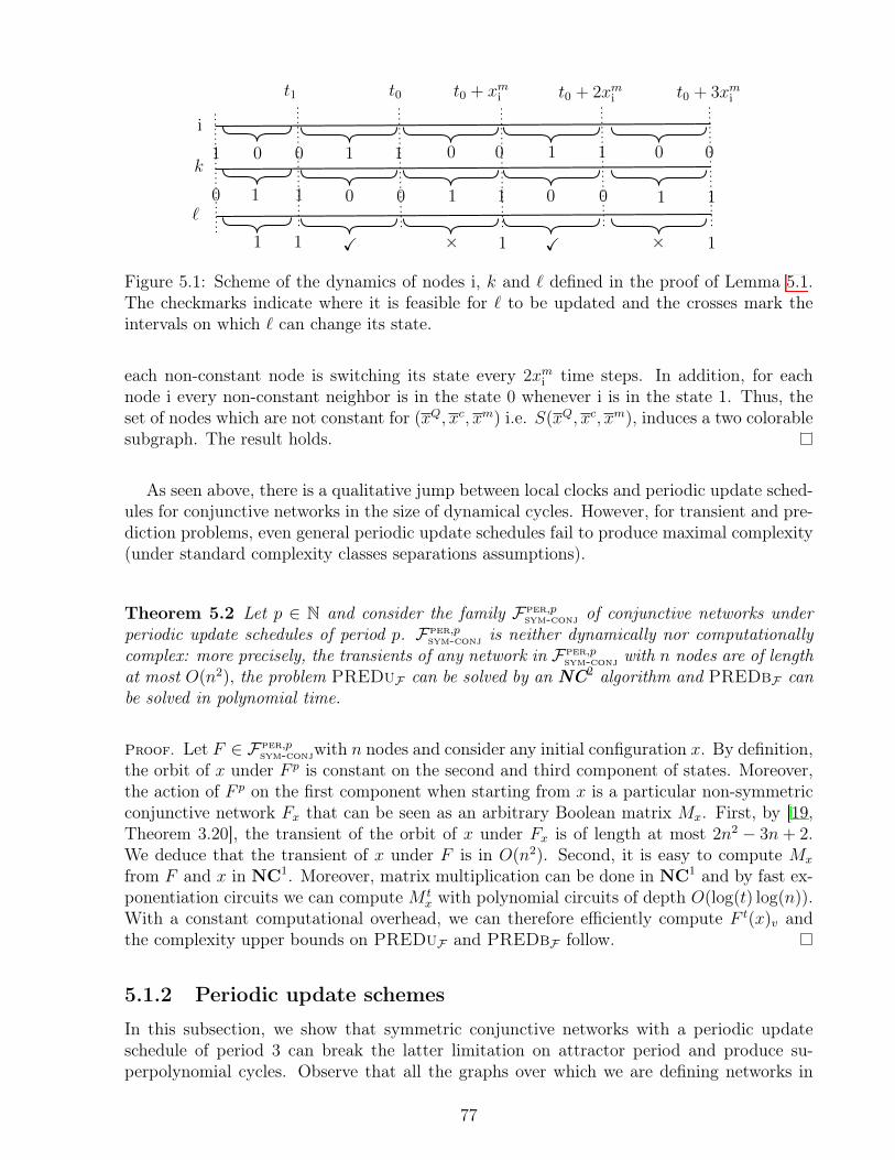
⇥XX ⇥

0

1

t0 + 3xmi

t0 + 2xmi

t0 + xmi

111 1

0

10

1

01

0

10 1

01 0 1

0

10

11

0

`

k

i

t0t1

Figure 5.1: Scheme of the dynamics of nodes i, k and ` defined in the proof of Lemma 5.1.The checkmarks indicate where it is feasible for ` to be updated and the crosses mark theintervals on which ` can change its state.

each non-constant node is switching its state every 2xmi

time steps. In addition, for eachnode i every non-constant neighbor is in the state 0 whenever i is in the state 1. Thus, theset of nodes which are not constant for (xQ, xc, xm

) i.e. S(xQ, xc, xm), induces a two colorable

subgraph. The result holds.

As seen above, there is a qualitative jump between local clocks and periodic update sched-ules for conjunctive networks in the size of dynamical cycles. However, for transient and pre-diction problems, even general periodic update schedules fail to produce maximal complexity(under standard complexity classes separations assumptions).

Theorem 5.2 Let p 2 N and consider the family Fper,psym-conj

of conjunctive networks underperiodic update schedules of period p. Fper,p

sym-conjis neither dynamically nor computationally

complex: more precisely, the transients of any network in Fper,psym-conj

with n nodes are of lengthat most O(n2

), the problem PREDuF can be solved by an NC2 algorithm and PREDbF can

be solved in polynomial time.

Proof. Let F 2 Fper,psym-conj

with n nodes and consider any initial configuration x. By definition,the orbit of x under F p is constant on the second and third component of states. Moreover,the action of F p on the first component when starting from x is a particular non-symmetricconjunctive network Fx that can be seen as an arbitrary Boolean matrix Mx. First, by [19,Theorem 3.20], the transient of the orbit of x under Fx is of length at most 2n2 � 3n+ 2.We deduce that the transient of x under F is in O(n2

). Second, it is easy to compute Mx

from F and x in NC1. Moreover, matrix multiplication can be done in NC

1 and by fast ex-ponentiation circuits we can compute M t

x with polynomial circuits of depth O(log(t) log(n)).With a constant computational overhead, we can therefore efficiently compute F t

(x)v andthe complexity upper bounds on PREDuF and PREDbF follow.

5.1.2 Periodic update schemes

In this subsection, we show that symmetric conjunctive networks with a periodic updateschedule of period 3 can break the latter limitation on attractor period and produce su-perpolynomial cycles. Observe that all the graphs over which we are defining networks in

77

this family (and also in the other concrete examples we will be exploring in next sections)are non-directed (symmetric). If we observe carefully the effect of periodic update schemes,we note that we are actually changing the interaction graph of the network by consideringdifferent orders for updating nodes and thus, breaking the symmetry in the different connec-tions that nodes have in the network. Moreover, we corroborate this remark by showing thatactually, we can simulate arbitrary conjunctive networks by using a periodic update scheme.We accomplish this by applying our formalism on simulation and gadget glueing. In fact,we show that the family of symmetric conjunctive networks admits coherent Gconj-gadgets.Thus it is capable of simulating the familly (Fconj,F⇤

conj). Particularly, this implies that this

family admits attractors of superpolynomial period.

Proposition 5.3 Let p � 1 and Fper,psym-conj

be the family of symmetric conjunctive networksunder periodic update schedule of period p. Fper,p

sym-conjis not universal and therefore it does

not admit coherent Gm-gadgets.

Proof. We actually show that the longest transient of any F 2 Fper,psym-conj

with n nodes isO(n2

), then the conclusions follow by Corollary 2.19 and Theorem 3.16. Recall that thealphabet is {0, 1}⇥ {0, . . . , p}⇥ 2

{0,...,p} and that, by definition, on any given configurationx the component {0, . . . , p}⇥ 2

{0,...,p} is periodic of period p independently of the behavioron the first {0, 1} component. Moreover, the behavior on the {0, 1} component is that of afixed (non-symmetric) conjunctive network F 0 in the following sense:

F t+p(x) = F 0

(F t(x)), 8t � 0.

By [19, Theorem 3.20], the transient of any orbit of F 0 is O(n2). We deduce that the transient

of the orbit of x under F is also O(n2).

Theorem 5.4 Let Fper,3sym-conj

be the family of symmetric conjunctive networks under periodicupdate schedules of period 3. Fper,3

sym-conjhas coherent Gconj-gadgets and therefore simulates

the family of conjunctive networks (Fconj,F⇤conj). In particular, it can produce attractors of

superpolynomial period.

Proof. We start by showing that Fper,3sym-conj

has the coherent Gconj-gadgets. We use thenotations from Definition 3.9. Let FCOPY 2 Fper,3

sym-conjbe defined on the following graph with

nodes VCOPY = {v1, v2, v3, v4, v5, v04, v05}:

v04

v05

v1 v2 v3

v4 v5

Let also FAND 2 Fper,3sym-conj

be defined on the following graph with nodesVAND = {v1, v2, v01, v02, v3, v4, v5}:

78

v01

v02

v1 v2v3 v4 v5

Recall that both FCOPY and FAND have alphabet Q = {0, 1}⇥ {0, 1, 2}⇥ 2{0,1,2}. Now let

C = Ci [ Co be the glueing interface with Ci = {i} and Co = {o}. FCOPY is seen as a gadgetwith one input and two outputs for the gate COPY 2 Gconj as follows:

• �i

COPY,1(i) = v2 and �i

COPY,1(o) = v1;• �o

COPY,1(i) = v5 and �oCOPY,1(o) = v4.

• �oCOPY,2(i) = v0

5and �o

COPY,2(o) = v04.

FAND is seen as a gadget with two inputs and one output for the gate AND 2 Gconj as follows:

• �i

AND,1(i) = v2 and �i

AND,1(o) = v1;• �i

AND,2(i) = v02

and �i

AND,2(o) = v01.

• �oAND,1(i) = v5 and �o

AND,1(o) = v4.

Note in particular that the conditions of Lemma 3.8 are satisfied so the closure by gadgetglueing of these gadgets stays in our family F . Indeed FCOPY has the same induced labelgraphs on all images of C under � maps, and the neighborhood of �i

COPY,1(Co) = v1 is v2which belongs to �i

COPY,1(C), and similarly for other � maps. Corresponding properties holdalso for FAND. We now define the following elements required by Definition 3.9:

• The two state configurations sq for q 2 {0, 1} are defined by sq(i) = (q, 0, {0, 2}) andsq(o) = (1, 0, {0, 1}).

• The context configuration is defined by c(v3) = (1, 0, {1, 2}) both for FCOPY and FAND.

• The time constant is T = 3.

• The standard trace ⌧q,q0 over the glueing interface from q 2 {0, 1} to q0 2 {0, 1} is givenby:

time i o0 (q, 0, {0, 2}) (1, 0, {0, 1})1 (1, 1, {0, 2}) (q, 1, {0, 1})2 (1, 2, {0, 2}) (1, 2, {0, 1})3 (q0, 0, {0, 2}) (1, 0, {0, 1})

.

• For any qi, qTi , qo, qo0 2 {0, 1} we have the following {v1, v5, v05}-pseudo orbit for FCOPY:

time v1 v2 v3 v4 v5 v04 v050 (qi, 0, {0, 2}) (1, 0, {0, 1}) (1, 0, {1, 2}) (qo, 0, {0, 2}) (1, 0, {0, 1}) (q0o, 0, {0, 2}) (1, 0, {0, 1})1 (1, 1, {0, 2}) (qi, 1, {0, 1}) (1, 1, {1, 2}) (1, 1, {0, 2}) (qo, 1, {0, 1}) (1, 1, {0, 2}) (q0o, 1, {0, 1})2 (1, 2, {0, 2}) (1, 2, {0, 1}) (qi, 2, {1, 2}) (1, 2, {0, 2}) (1, 2, {0, 1}) (1, 2, {0, 2}) (1, 2, {0, 1})3 (q0i , 0, {0, 2}) (1, 0, {0, 1}) (1, 0, {1, 2}) (qi, 0, {0, 2}) (1, 0, {0, 1}) (qi, 0, {0, 2}) (1, 0, {0, 1})

.

• For any qi, qTi , qi0 , qTi0, qo 2 {0, 1} we have the following {v1, v01, v5}-pseudo orbit for FAND:

79

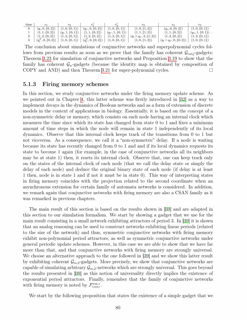
time v1 v2 v01 v02 v3 v4 v50 (qi, 0, {0, 2}) (1, 0, {0, 1}) (qi0 , 0, {0, 2}) (1, 0, {0, 1}) (1, 0, {1, 2}) (qo, 0, {0, 2}) (1, 0, {0, 1})1 (1, 1, {0, 2}) (qi, 1, {0, 1}) (1, 1, {0, 2}) (qi0 , 1, {0, 1}) (1, 1, {1, 2}) (1, 1, {0, 2}) (qo, 1, {0, 1})2 (1, 2, {0, 2}) (1, 2, {0, 1}) (1, 2, {0, 2}) (1, 2, {0, 1}) (qi ^ qi0 , 2, {1, 2}) (1, 2, {0, 2}) (1, 2, {0, 1})3 (qTi , 0, {0, 2}) (1, 0, {0, 1}) (qTi0 , 0, {0, 2}) (1, 0, {0, 1}) (1, 0, {1, 2}) (qi ^ qi0 , 0, {0, 2}) (1, 0, {0, 1})

.

The conclusion about simulations of conjunctive networks and superpolynomial cycles fol-lows from previous results as soon as we prove that the family has coherent Gconj-gadgets:Theorem 3.23 for simulation of conjunctive networks and Proposition 3.19 to show that thefamily has coherent Gw-gadgets (because the identity map is obtained by composition ofCOPY and AND) and then Theorem 3.21 for super-polynomial cycles.

5.1.3 Firing memory schemes

In this section, we study conjunctive networks under the firing memory update scheme. Aswe pointed out in Chapter 4, this latter scheme was firstly introduced in [32] as a way toimplement decays in the dynamics of Boolean networks and as a form of extension of discretemodels in the context of applications in biology. Essentially, it is based on the concept of anon-symmetric delay or memory, which consists on each node having an internal clock whichmeasures the time since which its state has changed from state 0 to 1 and fixes a minimumamount of time steps in which the node will remain in state 1 independently of its localdynamics. Observe that this internal clock keeps track of the transitions from 0 to 1 butnot viceversa. As a consequence, we call it a “non-symmetric” delay. If a node is waitingbecause its state has recently changed from 0 to 1 and and if its local dynamics requests itsstate to become 1 again (for example, in the case of conjunctive networks all its neighborsmay be at state 1) then, it resets its internal clock. Observe that, one can keep track onlyon the states of the internal clock of each node (that we call the delay state or simply thedelay of each node) and deduce the original binary state of each node (if delay is at least1 then, node is in state 1 and if not it must be in state 0). This way of interpreting statesin firing memory coincides with the projection related to the second coordinate when anasynchronous extension for certain family of automata networks is considered. In addition,we remark again that conjunctive networks with firing memory are also a CSAN family as itwas remarked in previous chapters.

The main result of this section is based on the results shown in [39] and are adapted inthis section to our simulation formalism. We start by showing a gadget that we use for themain result consisting in a small network exhibiting attractors of period 3. In [39] it is shownthat an analog reasoning can be used to construct networks exhibiting linear periods (relatedto the size of the network) and thus, symmetric conjunctive networks with firing memoryexhibit non-polynomial period attractors, as well as symmetric conjunctive networks undergeneral periodic update schemes. However, in this case we are able to show that we have farmore than that, and that conjunctive networks with firing memory are strongly universal.We choose an alternative approach to the one followed in [39] and we show this latter resultby exhibiting coherent Gm,2-gadgets. More precisely, we show that conjunctive networks arecapable of simulating arbitrary Gm,2-networks which are strongly universal. This goes beyondthe results presented in [39] as this notion of universality directly implies the existence ofexponential period attractors. Finally, remember that the family of conjunctive networkswith firing memory is noted by Ffir,⌧

conj.

We start by the following proposition that states the existence of a simple gadget that we

80

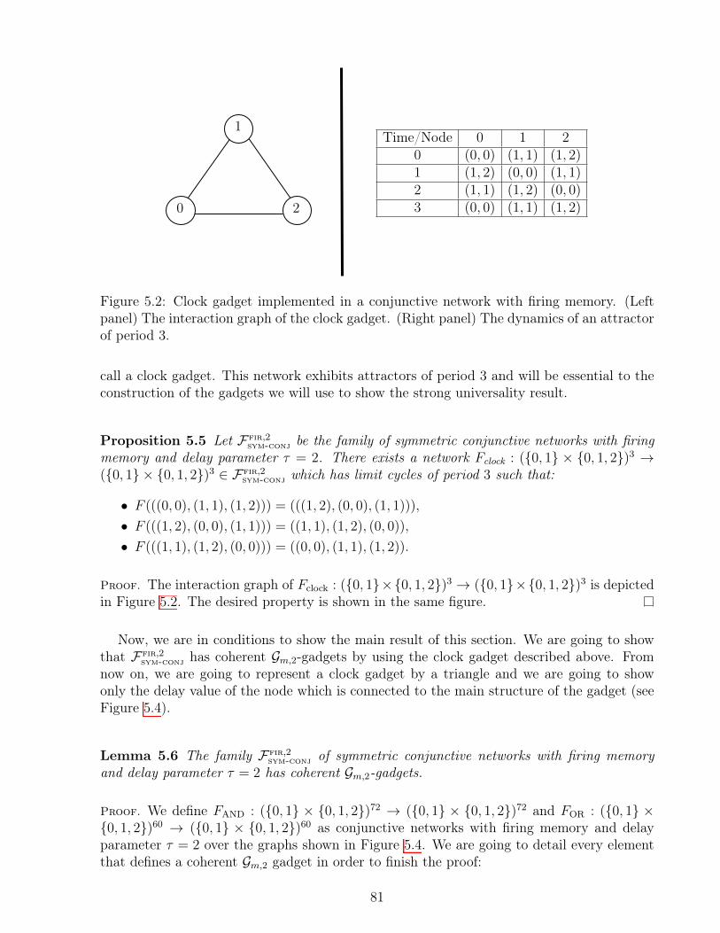
Time/Node 0 1 2

0 (0, 0) (1, 1) (1, 2)1 (1, 2) (0, 0) (1, 1)2 (1, 1) (1, 2) (0, 0)3 (0, 0) (1, 1) (1, 2)

1

20

Figure 5.2: Clock gadget implemented in a conjunctive network with firing memory. (Leftpanel) The interaction graph of the clock gadget. (Right panel) The dynamics of an attractorof period 3.

call a clock gadget. This network exhibits attractors of period 3 and will be essential to theconstruction of the gadgets we will use to show the strong universality result.

Proposition 5.5 Let Ffir,2sym-conj

be the family of symmetric conjunctive networks with firingmemory and delay parameter ⌧ = 2. There exists a network Fclock : ({0, 1} ⇥ {0, 1, 2})3 !({0, 1}⇥ {0, 1, 2})3 2 Ffir,2

sym-conjwhich has limit cycles of period 3 such that:

• F (((0, 0), (1, 1), (1, 2))) = (((1, 2), (0, 0), (1, 1))),

• F (((1, 2), (0, 0), (1, 1))) = ((1, 1), (1, 2), (0, 0)),

• F (((1, 1), (1, 2), (0, 0))) = ((0, 0), (1, 1), (1, 2)).

Proof. The interaction graph of Fclock : ({0, 1}⇥{0, 1, 2})3 ! ({0, 1}⇥{0, 1, 2})3 is depictedin Figure 5.2. The desired property is shown in the same figure.

Now, we are in conditions to show the main result of this section. We are going to showthat Ffir,2

sym-conjhas coherent Gm,2-gadgets by using the clock gadget described above. From

now on, we are going to represent a clock gadget by a triangle and we are going to showonly the delay value of the node which is connected to the main structure of the gadget (seeFigure 5.4).

Lemma 5.6 The family Ffir,2sym-conj

of symmetric conjunctive networks with firing memoryand delay parameter ⌧ = 2 has coherent Gm,2-gadgets.

Proof. We define FAND : ({0, 1} ⇥ {0, 1, 2})72 ! ({0, 1} ⇥ {0, 1, 2})72 and FOR : ({0, 1} ⇥{0, 1, 2})60 ! ({0, 1} ⇥ {0, 1, 2})60 as conjunctive networks with firing memory and delayparameter ⌧ = 2 over the graphs shown in Figure 5.4. We are going to detail every elementthat defines a coherent Gm,2 gadget in order to finish the proof:

81

1. We define the glueing surface C = Ci [ Co as Ci = {ci} [ {ci,1, ci,2, ci,3} and Co =

{c0o, co} [ {co0,1, co0,2, co0,3, } [ {co,1, co,2, co,3} as shown in Figure 5.3.2. The corresponding embedded copies of C in each gadget are shown in dashed boxes in

Figure 5.4 and the functions �i

FAND,k, �oFAND,k, �i

FOR,k and �oFOR,k for k = 1, 2 are defined

respecting the same order shown in Figure 5.3.3. For each x 2 {0, 1} we define the maps (see Figure 5.4):

• sx(ci) = 2x, (sx(ci,1), sx(ci,2), sx(ci,3) = (1, 0, 2);

• sx(c0o) = 1, (sx(c0o,1), sx(c0o,2), sx(c

0o,3) = (2, 0, 1); and

• sx(co) = 2, (sx(co,1), sx(co,2), sx(co,3) = (0, 1, 2).

4. Context configurations are shown in Figure 5.3 for every node that is not inside adashed box.

5. Each gadget takes T = 9 time steps to compute the simulation of an AND or an ORgate (See Figures 5.4 5.5, 5.6, 5.7, 5.8 and 5.9).

6. A standard trace and pseudo-orbit given by the dynamics shown in Figures 5.4 5.5,5.6, 5.7, 5.8 and 5.9. We remark that the function k(x, y) in Figure 5.9 is defined byk(0, 0) = 0, k(1, 0) = k(1, 1) = 2 and k(0, 1) = 1. Then, we have that k(x, y) is equalto OR(x, y) = 2(x_ y) with the exception that OR(1, 0) = 1. Thus, since the local ruleinterprets 2 and 1 as 1 (we recall that we are representing (1, 2) by 2 and (1, 1) by 1)and any node that changes its state to 1 updates its internal clock to 2, the gadgetcomputes 2(x _ y) in the next step of computation, as it is shown in Figure 5.9.

As a consequence of Lemma 5.6, we have the following theorem.

Theorem 5.7 The family Ffir,2sym-conj

of symmetric conjunctive networks with firing mem-ory and delay parameter ⌧ = 2 is strongly universal. In particular, it is dynamically andcomputationally complex.

Proof. Strong universality is a direct consequence of the capability of Ffir,2sym-conj

to simulatethe family �(Gm,2). This fact comes directly from the latter lemma, as Ffir,2

sym-conjis a CSAN

and has coherent Gm,2-gadgets. Thus, it simulates �(Gm,2) in constant time and linear space(see Corollary 3.12). Strong universality comes from the fact that �(Gm,2) is strongly universal(see Theorem 3.16). Finally, the complexity results (both dynamically and computationally)are a consequence of Corollary 2.14 and Theorem 2.18.

82

ci c0o co

C

Ci Co

ci,1

ci,2 ci,3 c0o,2

c0o,1

c0o,3co,2 co,3

co,1

Figure 5.3: The glueing interface considered for AND/OR gadgets implemented over a con-junctive network with firing memory. The labels given by marking functions ' are assignedin each gadget accordingly.

t = 0

21

1 2 0

2

2x 21

1 2 0

2

0

2 1

1 2

2y 21

1 2 0

2z 1

1 2

2

0

2z 1

1 2

2

0

t = 0

2 21

2x 21 1 2 0

1 2 0

2

12

1 2

2

1

2y 21

1 2 0

2z 1

1 2

2

0

2z 1

1 2

2

0

Figure 5.4: The initial condition and structure for AND/OR gadgets implemented overconjunctive networks with firing memory. (Upper panel) the AND gadget. (Bottom panel)the OR gadget. The variables (x, y) 2 {0, 1}2 represent the bits that the gadget is consideringas inputs and z 2 {0, 1} is a bit that is going to serve as an input for other gadget. Totalcomputation takes T = 9 time steps. The triangles represent clock gadgets. The dashed boxesmark the embedded copies of the glueing interface which plays the role of output/input.

83

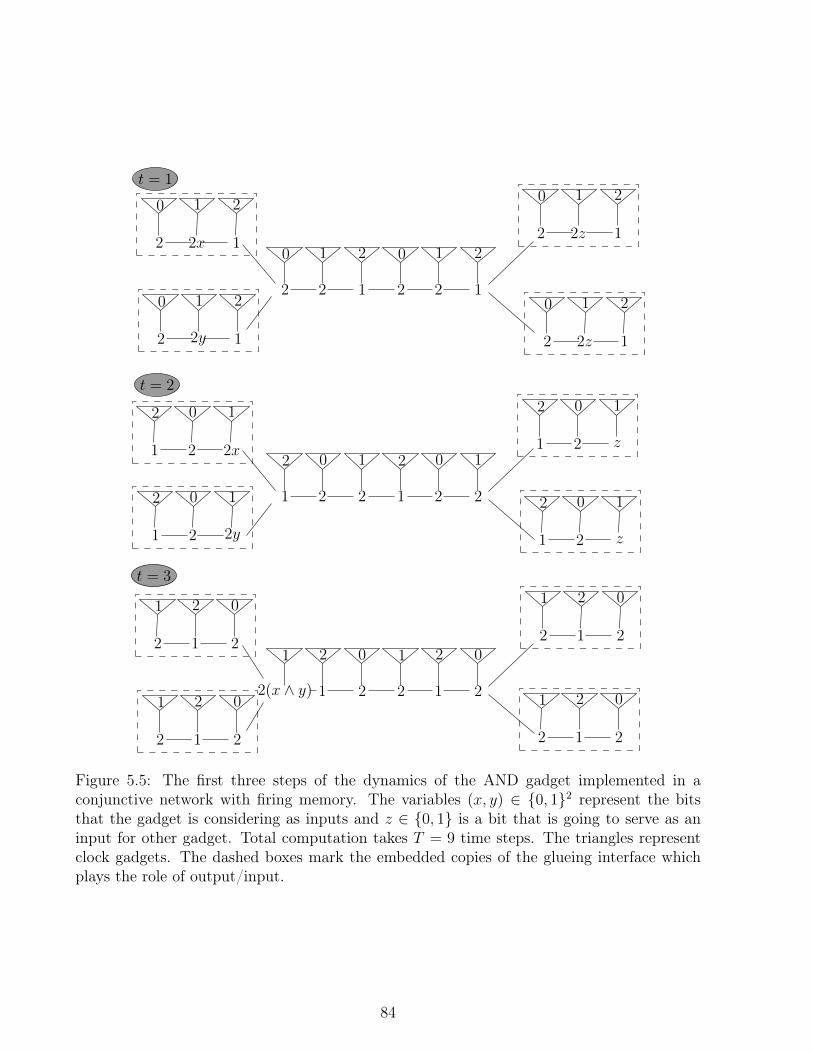
1 z2

2 0 1

1 z2

2 0 1

1 2y2

2 0 1

1 2x2

2 0 1

2 21

1 2 0

2 21

1 2 0

2 21

1 2 0

2 21

1 2 0

t = 3

t = 2

2 12y

0 1 2

2 12x

0 1 2

10

22

2

1

22

2 0 1

1 2

1

1 2

2 0

21

1 2 0

2(x ^ y) 2

0

2 1

1 2

t = 1

2 2z

0 1

2 2z

0 1

2

210

2 1

1

2

1

2

Figure 5.5: The first three steps of the dynamics of the AND gadget implemented in aconjunctive network with firing memory. The variables (x, y) 2 {0, 1}2 represent the bitsthat the gadget is considering as inputs and z 2 {0, 1} is a bit that is going to serve as aninput for other gadget. Total computation takes T = 9 time steps. The triangles representclock gadgets. The dashed boxes mark the embedded copies of the glueing interface whichplays the role of output/input.

84

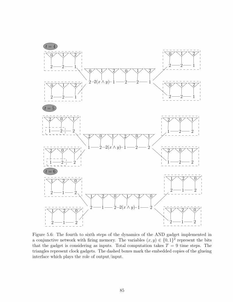
t = 4

t = 5

12(x ^ y)

0 1 2

2

2(x ^ y)2

2 0 1

1 2

1

1 2

2 0

1

2

2 2

0 1

1 22

2 0 1

1 22

2 0 1

1 22

2 0 1

1 22

2 0 1

2 12

0 1 2

2 12

0 1 2

2 12

0 1 2

2 12

0 1 2

t = 6

21

1 2 0

2

2 21

1 2 0

2 21

1 2 0

2 21

1 2 0

2 21

1 2 0

21

1 2 0

2(x ^ y)

Figure 5.6: The fourth to sixth steps of the dynamics of the AND gadget implemented ina conjunctive network with firing memory. The variables (x, y) 2 {0, 1}2 represent the bitsthat the gadget is considering as inputs. Total computation takes T = 9 time steps. Thetriangles represent clock gadgets. The dashed boxes mark the embedded copies of the glueinginterface which plays the role of output/input.

85

t = 7

t = 8

2(x ^ y)2

2 0 1

12

1

1 2

2 0

1 22

2 0 1

1 22

2 0 1

1 22

2 0 1

1 22

2 0 1

2 12

0 1 2

2 12

0 1 2

2 12

0 1 2

2 12

0 1 2

t = 9

21

1 2 0

2 2

0

2 1

1 2

2y0 21

1 2 0

2x0 21

1 2 0

2

210

2 1 12(x ^ y)

0 1 2

2

21

1 2 0

2(x ^ y)

21

1 2 0

2(x ^ y)

Figure 5.7: The final four steps of the dynamics of the AND gadget implemented in aconjunctive network with firing memory. The variables (x, y) 2 {0, 1}2 represent the bitsthat the gadget is considering as inputs. The variables (x0, y0) 2 {0, 1}2 represent the newinformation that the gadget is receiving as inputs. Total computation takes T = 9 time steps.The triangles represent clock gadgets. The dashed boxes mark the embedded copies of theglueing interface which plays the role of output/input.

86

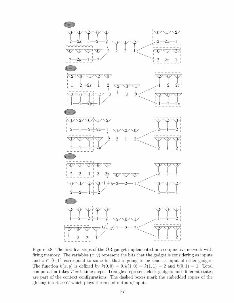
1 2z2

2 0 1

1 2z2

2 0 1

1 2y2

2 0 1

2 21

1 2 0

2 21

1 2 0

2 21

1 2 0

2 12

0 1 2

2 12

0 1 2

2 12

0 1 2

1 22

2 0 1

1 22

2 0 1

1 22

2 0 1 1 22

22 2 0 1

0 1

k(x, y)

21

2 0

1

2

1

2

2 12

2 12 0 1 2

0 1 2

1 + y

2x2

0 1

2

0

t = 2

t = 3

t = 4

t = 5

1 22

1 2x2 2 0 1

2 0 1

2

21

2 0

1

2

2 21

2 21 1 2 0

1 2 0

2

12x

1 2

2y

1

2 12z

0 1 2

2 12z

0 1 2

t = 1

2 12

2 12x 0 1 2

0 1 2

2

22

0 1

2

0

2 12y

0 1 2

Figure 5.8: The first five steps of the OR gadget implemented in a conjunctive network withfiring memory. The variables (x, y) represent the bits that the gadget is considering as inputsand z 2 {0, 1} correspond to some bit that is going to be send as input of other gadget.The function k(x, y) is defined by k(0, 0) = 0, k(1, 0) = k(1, 1) = 2 and k(0, 1) = 1. Totalcomputation takes T = 9 time steps. Triangles represent clock gadgets and different statesare part of the context configurations. The dashed boxes mark the embedded copies of theglueing interface C which plays the role of outputs/inputs.

87

t = 6

1

2

1

2

21

1 2

2

02

0211 2

1 22(x _ y)

2 21

1 2 0

2 21

1 2 0

2 21

1 2 0

2 12

0 1 2

2 12

0 1 2

t = 7

2 12(x _ y)

2 12 0 1 2

0 1 2

2

22

0 1

2

0

2 12

0 1 2

t = 8

1 2(x _ y)2

1 22 2 0 1

2 0 1

2

21

2 0

1

2

1 22

2 0 1

1 22

2 0 1

1 22

2 0 1

t = 9

2 21

2x0 21 1 2 0

1 2 0

2

12

1 2

2

1

2(x _ y) 21

1 2 0

2(x _ y) 21

1 2 0

2y0 21

1 2 0

Figure 5.9: The last four steps of the OR gadget implemented in a conjunctive network withfiring memory. The variables (x, y) represent the bits that the gadget is considering as inputsand (x0, y0) 2 {0, 1}2 correspond to new information that the gadget is interpreting as inputs.Total computation takes T = 9 time steps. Triangles represent clock gadgets and differentstates are part of the context configurations. The dashed boxes mark the embedded copiesof the glueing interface C which plays the role of outputs/inputs.

88

5.2 Locally positive symmetric signed conjunctive net-works

In this section, we study a generalization of conjunctive networks that we call locally positivesymmetric signed conjunctive networks. We denote this family by Flocally-pos. In this particularcase, we allow edges to have negative signs (which will switch the state of the correspondingneighbor) but with a local constraint: no neighborhood in which all the connections arenegative is allowed. More precisely, a locally positive symmetric conjunctive network is aCSAN (G,�, ⇢) in for any v 2 V (G) we have �v(q0, S) =

Vq2S

q and there exists w 2 N(v) :

⇢(vw) = Id.

We will show for this family that the threshold of universality when changing updatemodes is between block sequential update schemes and local clocks update schemes. Moreprecisely, we show, on one hand, that the family remains dynamically constrained under blocksequential schedule, and, on the other hand, we show that a local clocks version of this familyis strongly universal as a consequence of its capability of simulating coherent Gm,2-gadgets.

5.2.1 Block sequential update schemes

Theorem 5.8 Fix any b � 1 and consider Fblock,blocally-pos

the family of all locally positive sym-metric signed conjunctive networks under a block sequential schedule with at most b blocks.Any periodic orbit of any Fblock,b

locally-poshas period 1 or 2b.

Proof. Take some configuration x in a periodic orbit. If no node changes its state in theorbit then x is actually a fixed point. Otherwise take some node i that changes its state andconsider a maximal time interval I = [t1; t2] with t1 > 0 during which i is in state 0: 8t 2 I,F t

(x)i = 0 but F t1�1(x)i = F t2+1

(x)i = 1. Let j be any positive neighborhood (i.e. suchthat ⇢(i, j) is the identity). First, we must have that 8t 2 I, F t

(x)j = 1 because supposingF t

(x)i = F t(x)j = 0 implies F t0

(x)i = F t0(x)j = 0 for all t0 � t which would contradict the

hypothesis that i changes its state in the orbit. Thus t2 � t1 + 1 = b because it is by definitiona multiple of b and if it were strictly larger than b then node j would be updated in theinterval [t1; t2 � 1] and therefore would turn into state 0 in the interval I which has justbeen proven impossible. The same argument actually shows that i and j must be updatedsynchronously. Therefore it is updated at time t2 and we must have F t2+1

(x)j = 0. Thisimplies that F t2+b+1

(x)i = 0 and shows that the maximal time interval starting from t2 + 1

during which i is in state 1 is of length exactly b. We can then iterate this reasoning startingat time t2 + b+ 1 and we deduce that the orbit of x at node i alternates b steps in state 0

and b steps in state 1 forever. The same holds for any node that changes it state and finallywe have shown that the orbit of x is of period 1 or 2b.

5.2.2 Local clocks update schemes

We now turn to the main construction of this section. We recall the definition of a localclocks version of a certain family. We will call Fclock,c

locally-posthe family of all locally positive

symmetric conjunctive networks under local clocks update schemes with clock period c. A

89

local clock version of certain (G,�, ⇢) 2 Flocally-pos is a CSAN over the alphabet Qc =

Q⇥ {0, . . . , c� 1}⇥ {1, . . . , c} defined by:

�(v)((xQ)v, (xc)v, (xm)v), (xQ, xc, xm)|N(v))

=

((�(v)((xQ)v, xQ|N(i)), ( (xm)v

[(xc)v]) + 1 mod (xm)v, (xm)v) (xc)v = 0,

((xQ)v, ( (xm)v[(xc)v]) + 1 mod (xm)v, (xm)v) otherwise

where m(r) : {0, . . . , c� 1}! {0, . . . , c� 1} is such that m[r] =

(r if r m� 1,

m� 1 otherwise.

Now, we want to show that coherent AND/OR gadgets can be implemented in Fclock,clocally-pos

,i.e. we want to show that this family has coherent Gm,2 gadgets where Gm,2 = {AND2,OR2}where OR2 : {0, 1}2 ! {0, 1}2 is such that OR2(x, y) = (x _ y, x _ y) and the functionAND2 : {0, 1}2 ! {0, 1}2 is such that AND2(x, y) = (x ^ y, x ^ y). As a consequence, wewill have that Fclock,c

locally-posis strongly universal. However, in order to accomplish this task we

need a construction that we will be using for the next subsection. In particular, we need toimplement the gadgets that are shown in Figures 5.16 and 5.17. Then, we will adapt themin order to make them work for locally positive symmetric conjunctive networks.

Since the results on general signed symmetric conjunctive networks are required first inorder to show the proof of the main theorem of this section, we will just state the main resultand then, we will show the proof of Theorem 5.9 below in the next section, for sake of clarity.Doing so, we respect the hierarchical order between families and preserve coherence of resultsat the same time.

Theorem 5.9 There exists c > 0 such that the family Fclock,clocally-pos

of all locally positivesymmetric conjunctive networks under local clocks update scheme with clock parameter c hascoherent Gm,2-gadgets.

Corollary 5.10 below is a direct consequence of Theorem 5.9.

Corollary 5.10 There exists c > 0 such that the family Fclock,clocally-pos

of all locally positivesymmetric conjunctive networks under local clocks update scheme with clock parameter cis strongly universal. In particular, Fclock,c

locally-posis both dynamically and computationally

complex.

Proof. Proof is a direct consequence of Theorem 2.18, Corollary 2.14 and Corollary 3.18.

5.3 Symmetric signed conjunctive networksIn this section we study symmetric signed conjunctive networks with no label constrainton edges. Formally the symmetric signed conjunctive networks family is a CSAN family in{0, 1} in which �v : Q ⇥ 2

Q ! Q is given by �(q, S) = 0 if 0 2 S and �(q, S) = 1 if 0 62S and for any e 2 E we have ⇢e 2 {Id, Switch} where Switch(x) = 1 � x. When an

90

edge is labeled by Id we say that it is a positive edge and when it is labeled by Switchwe say that the edge is negative. We denote this family by Fsign-sym-conj and we considerFblock,b

sign-sym-conj,Fclock,c

sign-sym-conjand Fper,p

sign-sym-conjfor block sequential, local clocks and periodic

versions of this family respectively.

We start by remarking that for the parallel update scheme, Fsign-sym-conj family is notuniversal since it is a type of threshold family and thus it has bounded period attractors(see [42]). Then, a natural question is whether this remains true for other update schemes.We are going to show that, Fsign-sym-conj becomes strongly universal from block sequentialupdate schemes. We recall that in Fblock,b

sign-sym-conj, local functions are modified by adding an

internal clock. Each internal clock has the same period but a different initial shift. Thus, asexplained in Chapter 4, a block sequential scheme on a network can be viewed as an orderedpartition of its nodes into b blocks, such that the nodes belonging to a block are updatedin parallel while the blocks are iterated sequentially. More precisely, we have the followingdefinition:

�(v)(((xQ)v, (xb)v)(xQ, xb)|N(v)) =

((�(v)((xQ)v, xQ|N(i)), (xb)v � 1 mod b) if (xb)v = 0

((xQ)v, (xb)v � 1 mod b) otherwise.

5.3.1 Block sequential update schemes

In this section, we will show that Fblock,bsign-sym-conj

is strongly universal as a consequence of itscapability to implement coherent Gm,2-gadgets. In addition, we conclude that, as a directconsequence of the latter property, that previous family is both dynamically complex andcomputationally complex. This means that for this family, complex behavior is exhibitedunder block sequential update schemes.

We start by showing this less powerful result: Fblock,bsign-sym-conj

is able to simulate Gw-networks.This is only a way to motivate our main result and to show how key structures work in aparticular simple context. We do not use exactly this result in the actual proof of the maintheorem but we apply the same type of ideas since the related structures are part of thegadgets we construct which have only negative labels, i.e. each edge is labeled by the Switchfunction.

Lemma 5.11 The familly Fblock,3sign-sym-conj

of all signed symmetric conjunctive networks underblock sequential update schemes of at most 3 blocks has coherent Gw-gadgets.

Proof. We define a gadget simulating Id by considering two copies of the NOT gadget pre-sented in Figures 5.10 and 5.11. Observe that this gadget has 3 central nodes (marked insidea thick dotted rectangle in Figures 5.10 and 5.11) together with 2 copies of a 4 nodes cyclegraph. Generally speaking, the dynamics on these cycle graphs works as a clock which al-lows information to flow through the central part in only one direction (from left to right).In addition, they allow the gadget to erase information once it has been transmitted. Thislatter property allows the gadget to clean itself in order to receive new information. The wire

91

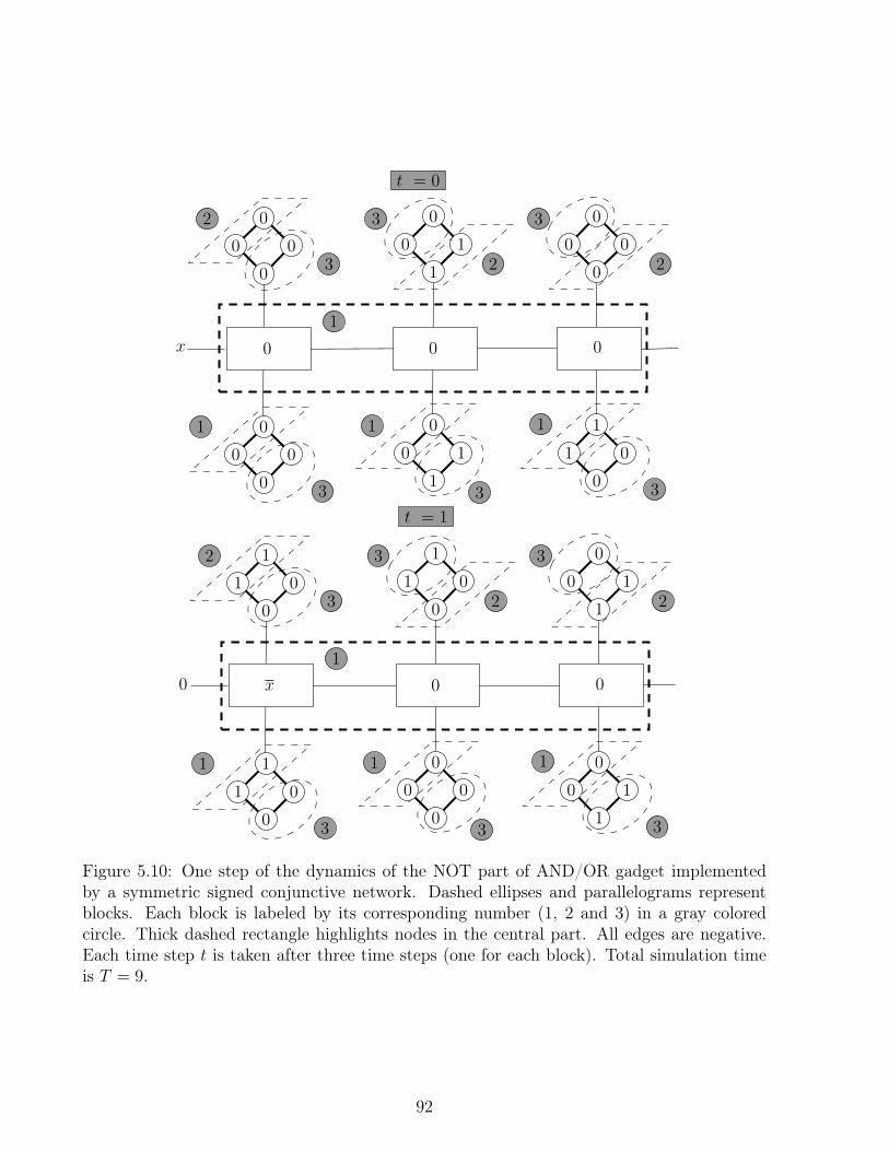
0

0

0

0

0

0

0

0

1

0

0

1

1

1

0

0

0

1

1

0

0

0

0

0

t = 0

0 0 0

1

2

1 1 1

22

3

3 33

x

3

3

0

1

1

0

1

1

0

0

0

0

0

0

0

0

1

1

1

0

0

1

1

1

0

0

x 0 0

1

2

1 1 1

22

3

3 33

3

3

t = 1

0

Figure 5.10: One step of the dynamics of the NOT part of AND/OR gadget implementedby a symmetric signed conjunctive network. Dashed ellipses and parallelograms representblocks. Each block is labeled by its corresponding number (1, 2 and 3) in a gray coloredcircle. Thick dashed rectangle highlights nodes in the central part. All edges are negative.Each time step t is taken after three time steps (one for each block). Total simulation timeis T = 9.

92

3

3

3 33

3

2 2

111

2

1

0x0

0

0

1

1

0

0

0

0

0

0

0

0

0

1

1

0

1

1

0

0

1

0

0

1

t = 2

0

3

3

x0

3 33

3

2 2

111

2

1

x00

0

0

0

0

0

1

1

0

1

1

0

0

1

0

0

1

0

0

0

0

0

0

0

0

t = 3

Figure 5.11: Two last steps of the dynamics described by the NOT part of AND/OR gadgetsimplemented by a symmetric signed conjunctive network. Dashed ellipses and parallelogramsrepresent blocks. Each block is labeled by its corresponding number (1, 2 and 3) in a graycolored circle. Thick dashed rectangle highlights nodes in the central part. All edges arenegative. Each time step t is taken after three time steps (one for each block). Totalsimulation time is T = 9.

93

NOT NOT

Figure 5.12: Wire gadget implemented on a signed symmetric conjuntive network. 2 copiesof NOT gadget are combined in order to form a wire. Simulation time is T = 6⇥ 3.

gadget is composed by two copies of the NOT gadget as is presented in Figure 5.12. Sincethis gadget is composed by two copies of the NOT gadget, this gadget is defined by a pathgraph with 6 central nodes together with 2 ⇥ 2 ⇥ 3 = 12 cycle graphs (two copies for eachnode). We enumerate nodes in the central part from left to right by the following ordering:{0, 1, 2, 3, 4, 5}. Additionally, since the functioning of each copy of the NOT gadget is basedin an ordered partition of 3 blocks, we take the union of the corresponding blocks on eachpartition in order to define 3 larger blocks for the wire gadget. For one of this larger blockswe use the notation {0, 1, 2}. Thus, observe that each wire takes T = 6⇥ 3 = 18 time stepsin order transport the information. This is because for each round of 3 time steps in whichwe update each block, we make the signal pass through exactly one node. We define theglueing interface as Ci = {i} and Co = {o}. We map input and output in the following way:�i(i) = 1, �i

(o) = 0, �o(i) = {5} �o

(o) = {4}. Note that in each case the neighborhood ofoutput and input part is completely contained in Ci and Co respectively and also the imageof C by functions � is always the same (two nodes path graph). Thus, the glueing interfacesatisfies conditions of Lemma 3.8. Now we enumerate the remaining elements required byDefinition 3.9:

• State configurations sq(i) = (q, 0) and sq(o) = (q, 1) for any q 2 {0, 1}.• Context configurations are given in Figure 5.10 as well as the iteration order which

defines the blocks.• Standard trace and pseudo orbit for nodes {0, 1, 4, 5} are defined in Figure 5.10 and

Figure 5.11.

We are now in conditions to introduce the main result of this section:

Lemma 5.12 The familly Fblock,3sign-sym-conj

of all signed symmetric conjunctive networks underblock sequential update schemes of at most 3 blocks has coherent Gm,2-gadgets.

Proof. We will show that the gadgets in the Figures 5.16 and 5.17 are coherent Gm,2-gadgets.Note that both these gadgets are made of several wires made of NOT gadgets (we call thetwo in the left hand side of the figure input wires and the other two at the right hand sideoutput wires) and a computation gadget. Observe that, each of these structures (wires andcomputation gadget) needs exactly 3 blocks. In addition, note that in Table 5.4 the dynamicsof the 4-cycles that are attached to each node is shown. We recall that the function ofthese clocks is to allow information to flow in one direction only (all the interactions aresymmetric so this is not straightforward) and to erase information once it has been copiedor processed by the nodes in the gadget. We use the following notation in order to represent

94

nodes in these structures: cs,i,j,p where s is the number of the NOT gadget (a 3-node-pathtogether with two 4-cycles for each node, see Figure 5.13) to which the cycle is attached, sos 2 {1, 2, 3, 4, 5, 6, 7, 8, 9} where the order is taken from left to right (for example in Figure5.16 the copy associated to (v1, v2, v3) comes first then, (v0

1, v0

2, v0

3), then (v4, v5, v6) and so

on). Additionally, i is in the position of the cycle in the NOT block, so i 2 {1, 2, 3}, j is theposition of the node relative to the 4-cycle graph considered in counter clockwise order (seeFigure 5.13), so j 2 {1, 2, 3, 4} and p is the position of the cycle in the central structure ofthe gadget. Observe that, since there are two copies for each node, we denote them by upperand lower so p 2 {u, l}. Since input wires and output wires are needed to be updated at thesame time and are independent (we have two copies for each one) we combine their blocksin the obvious way (we take the union of pairs of blocks that have the same update order).More precisely, we combine 3 ⇥ 9 blocks of each particular part (there are 8 copies of NOTand one computation gadget having 3 blocks each one) in order to define again only 3 blocks.The precise definition, using notation shown in Figures 5.16 and 5.17, is the following:

• B0 =

12Si=1

{vi} [ {v0i} [

Ss,i{cs,i,1,l, cs,i,2,l};

• B1 =Ss{cs,1,3,u, cs,1,4,u, cs,2,1,u, cs,2,2,u, cs,3,1,u, cs,3,2,u}; and

• B2 =Ss,i{cs,i,3,l, cs,i,4,l}.

Now we are going to use information in Tables 5.2, 5.3 and 5.4 in order to show that thesegadgets satisfy the conditions of Definition 3.9. Observe that, on the one hand, for the ORgadget (see Figure 5.16), input wires compute the result in 3⇥ 3 (it needs to carry the signalthrough the three nodes in the wire and each of this intermediate steps takes three steps, onefor each block) time steps and computation gadget takes 3 ⇥ 3 as well. On the other hand,for the AND gadget (see Figure 5.17) input wires compute the result in 3⇥ 6 time steps. Wedefine the associated network as FAND : ({0, 1}⇥ {0, 1, 2})15⇥2⇥4 ! ({0, 1}⇥ {0, 1, 2})15⇥2⇥4

and FOR : ({0, 1}⇥ {0, 1, 2})15⇥2⇥4 ! ({0, 1}⇥ {0, 1, 2})15⇥2⇥4. In fact we have that:

1. There is a unique glueing interface given by C = Ci [ Co where:• Ci = {i} [ {a(i, 1), a(i, 2), a(i, 3), a(i, 4)} [ {a0(i, 1), a0(i, 2), a0(i, 3), a0(i, 4)}; and• Co = {o0, o}[ {a(o0, 1), a(o0, 2), a(o0, 3), a(o0, 4)}[ {a(o, 1), a(o, 2), a(o, 3), a(o, 4)}[{a0(o0, 1), a0(o0, 2), a0(o0, 3), a0(o0, 4)} [ {a0(o, 1), a0(o, 2), a0(o, 3), a0(o, 4)}

We define the labelling functions �i

AND,k, �oAND,k, �i

OR,k, �oOR,k (for the sake of simplicity

we show the definition for the AND gadget since the one for the OR gadget is completelyanalogous) for k = 1, 2 as:

• �i

AND,1(i) = v1, �i

AND,1(o0) = v2 and �i

AND,1(o) = v3;

• �i

AND,1(a(i, r)) = c1,1,r,u, �i

AND,1(a0(i, r)) = c1,1,r,l for r = 1, 2, 3, 4, where 1 corre-

sponds to the NOT gadget which starts with v1 in Figure 5.17.• �i

AND,1(a(o0, r)) = c1,2,r,u, �i

AND,1(a0(o0, r)) = c1,2,r,l for r = 1, 2, 3, 4, where 1 corre-

sponds to the NOT gadget which starts with v1 in Figure 5.17;• �i

AND,1(a(o, r)) = c1,3,r,u, �i

AND,1(a0(o, r)) = c1,3,r,l for r = 1, 2, 3, 4, where 1 corre-

sponds to the NOT gadget which starts with v01

in Figure 5.17;• �i

AND,2(i) = v01, �i

AND,2(o0) = v0

2and �i

AND,2(o) = v03;

95

• �i

AND,2(a(i, r)) = c10,1,r,u, �i

AND,1(a0(i, r)) = c10,1,r,l for r = 1, 2, 3, 4, where 2 corre-

spond to the NOT gadget which starts with v01

in Figure 5.17;• �i

AND,2(a(o0, r)) = c10,2,r,u, �i

AND,1(a0(o0, r)) = c10,2,r,l for r = 1, 2, 3, 4, where 2

corresponds to the NOT gadget which starts with v01

in Figure 5.17;• �i

AND,2(a(o, r)) = c10,3,r,u, �i

AND,1(a0(o, r)) = c10,3,r,l for r = 1, 2, 3, 4, where 2 corre-

sponds to the NOT gadget which starts with v01

in Figure 5.17.• �o

AND,1(i) = v10, �oAND,1(o

0) = v11 and �o

AND,1(o) = v12;

• �oAND,1(a(i, r)) = c5,1,r,u, �o

AND,1(a0(i, r)) = c5,1,r,l for r = 1, 2, 3, 4, where 8 corre-

sponds to the NOT gadget which starts with v10 in Figure 5.17.• �o

AND,1(a(o0, r)) = c5,2,r,u, �o

AND,1(a0(o0, r)) = c5,2,r,l for r = 1, 2, 3, 4, where 8 corre-

sponds to the NOT gadget which starts with v10 in Figure 5.17;• �o

AND,1(a(o, r)) = c5,3,r,u, �oAND,1(a

0(o, r)) = c5,3,r,l for r = 1, 2, 3, 4, where 8 corre-

sponds to the NOT gadget which starts with v10 in Figure 5.17;• �o

AND,2(i) = v010

, �oAND,2(o

0) = v0

11and �o

AND,2(o) = v012;

• �i

AND,2(a(i, r)) = c50,1,r,u, �i

AND,2(a0(i, r)) = c50,1,r,l for r = 1, 2, 3, 4, where 9 corre-

spond to the NOT gadget which starts with v010

in Figure 5.17;• �o

AND,2(a(o0, r)) = c50,2,r,u, �o

AND,2(a0(o0, r)) = c50,2,r,l for r = 1, 2, 3, 4, where 9

corresponds to the NOT gadget which starts with v10 in Figure 5.17;• �o

AND,2(a(o, r)) = c50,3,r,u, �oAND,2(a

0(o, r)) = c50,3,r,l for r = 1, 2, 3, 4, where 9 corre-

sponds to the NOT gadget which starts with v010

in Figure 5.17.2. State configurations are defined for each q 2 {0, 1} as sq(i) = (q, 1) and sq(o0) = sq(o) =

(0, 1) and the state configuration of the nodes in the clocks i.e. the ones labeled by aare constant and shown in Table 5.4. The block number for each of these nodes can isthe same as the original NOT gadget 5.10.

3. Context configurations are described in Tables 5.2, 5.3 and 5.4 as the ones related tothe cycles of length 4 connected to central path of the gadgets and nodes in the pathwhich are not part of the glueing interface.

4. Standard trace is defined in Tables 5.2 and 5.3 (which contain the information relatedto the dynamics of nodes v1, v01, v2, v

02, v3, v03, v10, v

010, v11, v011, v12, v

012

) and in Table 5.4(which contains the dynamics of the nodes in the 4-cycles).

5. Simulation constant is T = 3⇥ 12 as it is shown in Tables 5.2,5.3 and6. Pseudo-orbit is given by the dynamics shown in in Tables 5.2, 5.3, and 5.4 where

x, y, x0, y0, z are variables.

Corollary 5.13 The familly Fblock,2sign-sym-conj

of all signed symmetric conjunctive networks un-der block sequential update schemes with at most 3 blocks is strongly universal. In particular,it is both dynamically and computationally complex.

Proof. Strong universality holds from the fact that family is capable of simulating Gm,2 inlinear space and constant time (see Corollary 3.18). The family is dynamically and com-

96

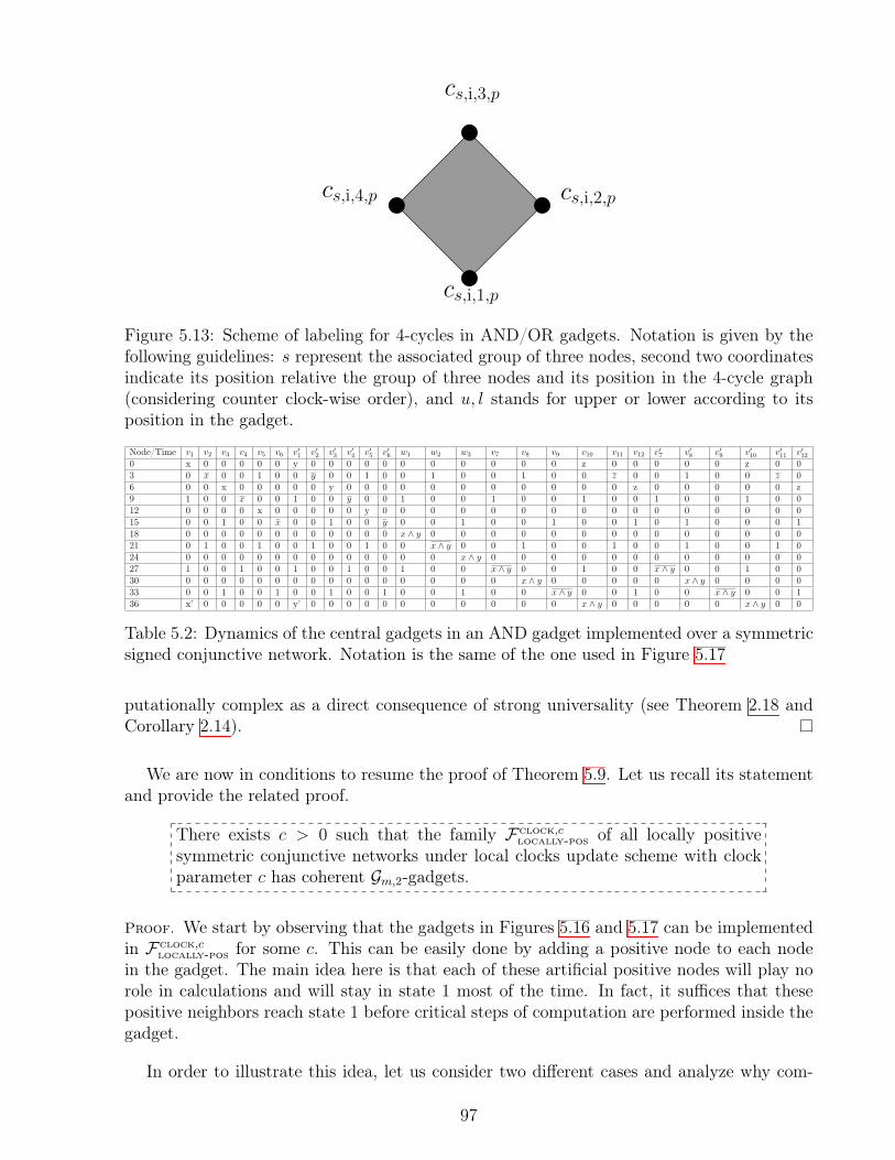
cs,i,1,p

cs,i,2,p

cs,i,3,p

cs,i,4,p

Figure 5.13: Scheme of labeling for 4-cycles in AND/OR gadgets. Notation is given by thefollowing guidelines: s represent the associated group of three nodes, second two coordinatesindicate its position relative the group of three nodes and its position in the 4-cycle graph(considering counter clock-wise order), and u, l stands for upper or lower according to itsposition in the gadget.

Node/Time v1 v2 v3 v4 v5 v6 v01

v02

v03

v04

v05

v06

w1 w2 w3 v7 v8 v9 v10 v11 v12 v07

v08

v09

v010

v011

v012

0 x 0 0 0 0 0 y 0 0 0 0 0 0 0 0 0 0 0 z 0 0 0 0 0 z 0 03 0 x 0 0 1 0 0 y 0 0 1 0 0 1 0 0 1 0 0 z 0 0 1 0 0 z 06 0 0 x 0 0 0 0 0 y 0 0 0 0 0 0 0 0 0 0 0 z 0 0 0 0 0 z9 1 0 0 x 0 0 1 0 0 y 0 0 1 0 0 1 0 0 1 0 0 1 0 0 1 0 012 0 0 0 0 x 0 0 0 0 0 y 0 0 0 0 0 0 0 0 0 0 0 0 0 0 0 015 0 0 1 0 0 x 0 0 1 0 0 y 0 0 1 0 0 1 0 0 1 0 1 0 0 0 118 0 0 0 0 0 0 0 0 0 0 0 0 x ^ y 0 0 0 0 0 0 0 0 0 0 0 0 0 021 0 1 0 0 1 0 0 1 0 0 1 0 0 x ^ y 0 0 1 0 0 1 0 0 1 0 0 1 024 0 0 0 0 0 0 0 0 0 0 0 0 0 0 x ^ y 0 0 0 0 0 0 0 0 0 0 0 027 1 0 0 1 0 0 1 0 0 1 0 0 1 0 0 x ^ y 0 0 1 0 0 x ^ y 0 0 1 0 030 0 0 0 0 0 0 0 0 0 0 0 0 0 0 0 0 x ^ y 0 0 0 0 0 x ^ y 0 0 0 033 0 0 1 0 0 1 0 0 1 0 0 1 0 0 1 0 0 x ^ y 0 0 1 0 0 x ^ y 0 0 136 x’ 0 0 0 0 0 y’ 0 0 0 0 0 0 0 0 0 0 0 x ^ y 0 0 0 0 0 x ^ y 0 0

Table 5.2: Dynamics of the central gadgets in an AND gadget implemented over a symmetricsigned conjunctive network. Notation is the same of the one used in Figure 5.17

putationally complex as a direct consequence of strong universality (see Theorem 2.18 andCorollary 2.14).

We are now in conditions to resume the proof of Theorem 5.9. Let us recall its statementand provide the related proof.

There exists c > 0 such that the family Fclock,clocally-pos

of all locally positivesymmetric conjunctive networks under local clocks update scheme with clockparameter c has coherent Gm,2-gadgets.

Proof. We start by observing that the gadgets in Figures 5.16 and 5.17 can be implementedin Fclock,c

locally-posfor some c. This can be easily done by adding a positive node to each node

in the gadget. The main idea here is that each of these artificial positive nodes will play norole in calculations and will stay in state 1 most of the time. In fact, it suffices that thesepositive neighbors reach state 1 before critical steps of computation are performed inside thegadget.

In order to illustrate this idea, let us consider two different cases and analyze why com-

97

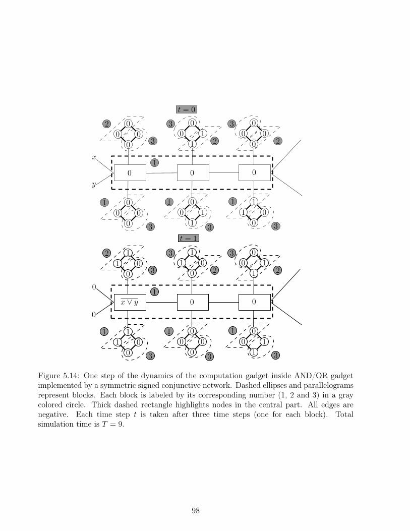
0

0

0

0

0

0

0

0

1

0

0

1

1

1

0

0

0

1

1

0

0

0

0

0

t = 0

0 0 0

1

2

1 1 1

22

3

3 33

x

y

3

3

0

1

1

0

1

1

0

0

0

0

0

0

0

0

1

1

1

0

0

1

1

1

0

0

x _ y 0 0

1

2

1 1 1

22

3

3 33

0

0

3

3

t = 1

Figure 5.14: One step of the dynamics of the computation gadget inside AND/OR gadgetimplemented by a symmetric signed conjunctive network. Dashed ellipses and parallelogramsrepresent blocks. Each block is labeled by its corresponding number (1, 2 and 3) in a graycolored circle. Thick dashed rectangle highlights nodes in the central part. All edges arenegative. Each time step t is taken after three time steps (one for each block). Totalsimulation time is T = 9.

98

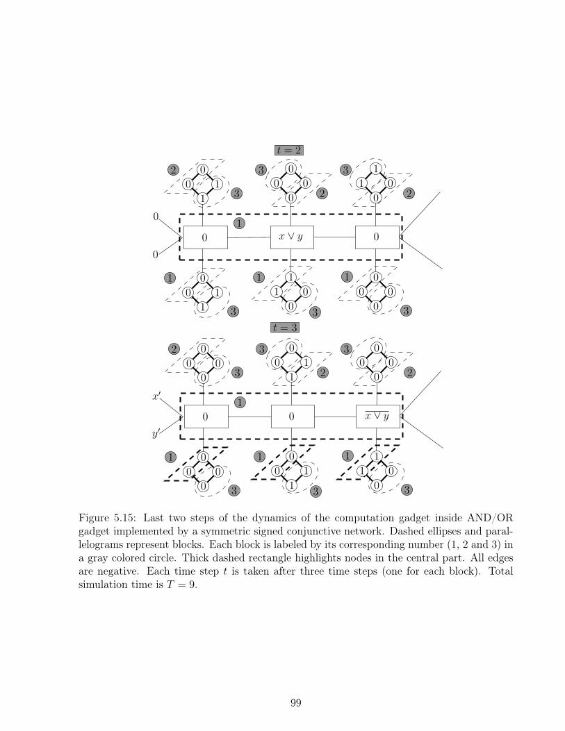
3

3

0

0

3 33

3

2 2

111

2

1

0x _ y0

0

0

1

1

0

0

0

0

0

0

0

0

0

1

1

0

1

1

0

0

1

0

0

1

t = 2

3

3

y0

x0

3 33

3

2 2

111

2

1

x _ y00

0

0

0

0

0

1

1

0

1

1

0

0

1

0

0

1

0

0

0

0

0

0

0

0

t = 3

Figure 5.15: Last two steps of the dynamics of the computation gadget inside AND/ORgadget implemented by a symmetric signed conjunctive network. Dashed ellipses and paral-lelograms represent blocks. Each block is labeled by its corresponding number (1, 2 and 3) ina gray colored circle. Thick dashed rectangle highlights nodes in the central part. All edgesare negative. Each time step t is taken after three time steps (one for each block). Totalsimulation time is T = 9.

99

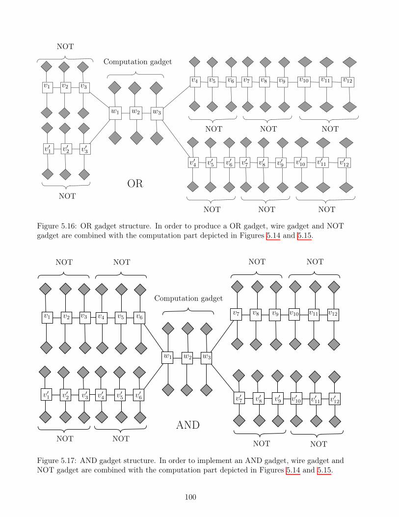
v01

v02 v0

3

w1 w2 w3

v07

v08 v0

9v04

v05

v06

NOT

NOT NOT

NOT

Computation gadget

OR

v1 v2 v3v7 v8 v9v4 v5 v6

NOT NOT

v10 v11 v12

NOT

v010

v011 v0

12

NOT

Figure 5.16: OR gadget structure. In order to produce a OR gadget, wire gadget and NOTgadget are combined with the computation part depicted in Figures 5.14 and 5.15.

v09

v08

v07

v9v8v7

w3w2w1

v03

v02

v01 v0

6v05

v04

v3v2v1 v6v5v4

NOTNOTNOT

NOT

Computation gadget

NOTNOTAND

v012

v011

v010

NOT

v12v11v10

NOT

Figure 5.17: AND gadget structure. In order to implement an AND gadget, wire gadget andNOT gadget are combined with the computation part depicted in Figures 5.14 and 5.15.

100

Node/Time v1 v2 v3 v01

v02

v03

w1 w2 w3 v4 v5 v6 v7 v8 v9 v10 v11 v12 v04

v05

v06

v07

v08

v09

v010

v011

v012

0 x 0 0 y 0 0 0 0 0 0 0 0 0 0 0 z 0 0 0 0 0 0 0 0 z 0 03 0 x 0 0 y 0 0 1 0 0 1 0 0 1 0 0 z 0 0 1 0 0 1 0 0 z 06 0 0 x 0 0 y 0 0 0 0 0 0 0 0 0 0 0 z 0 0 0 0 0 0 0 0 z9 1 0 0 1 0 0 x _ y 0 0 1 0 0 1 0 0 1 0 0 1 0 0 1 0 0 1 0 012 0 0 0 0 0 0 0 x _ y 0 0 0 0 0 0 0 0 0 0 0 0 0 0 0 0 0 0 015 0 0 1 0 0 1 0 0 x _ y 0 0 1 0 0 1 0 0 1 0 1 0 0 1 0 0 1 018 0 0 0 0 0 0 0 0 0 x _ y 0 0 0 0 0 0 0 0 x _ y 0 0 0 0 0 0 0 021 0 1 0 0 1 0 0 1 0 0 x _ y 0 0 1 0 0 1 0 0 x _ y 0 0 1 0 0 1 024 0 0 0 0 0 0 0 0 0 0 0 x _ y 0 0 0 0 0 0 0 0 x _ y 0 0 0 0 0 027 1 0 0 1 0 0 1 0 0 1 0 0 x _ y 0 0 1 0 0 1 0 0 x _ y 0 0 1 0 030 0 0 0 0 0 0 0 0 0 0 0 0 0 x _ y 0 0 0 0 0 0 0 0 x _ y 0 0 0 033 0 0 1 0 0 1 0 0 1 0 0 1 0 0 x _ y 0 0 1 0 0 1 0 0 x _ y 0 0 136 x’ 0 0 y’ 0 0 0 0 0 0 0 0 0 0 0 x _ y 0 0 0 0 0 0 0 0 x _ y 0 0

Table 5.3: Dynamics for central gadgets in OR gadget implemented over a symmetric signedconjunctive network. Notation is the same of the one shown in Figure 5.16

Node/Time cs,1,1,u cs,1,2,u cs,1,3,u cs,1,4,u cs,2,1,u cs,2,2,u cs,2,3,u cs,2,4,u cs,3,1,u cs,3,2,u cs,3,3,u cs,3,4,u0 0 0 1 1 0 0 1 1 1 1 0 03 1 1 0 0 0 0 0 0 0 0 1 16 0 0 0 0 1 1 0 0 0 0 0 09 0 0 1 1 0 0 1 1 1 1 0 0Node/Time cs,1,1,l cs,1,2,l cs,1,3,l cs,1,4,l cs,2,1,l cs,2,2,l cs,2,3,l cs,2,4,l cs,3,1,l cs,3,2,l cs,3,3,b cs,3,4,b0 1 1 0 0 0 0 0 0 0 0 1 13 0 0 1 1 1 1 0 0 0 0 0 06 0 0 0 0 0 0 1 1 1 1 0 09 1 1 0 0 0 0 0 0 0 0 1 1

Table 5.4: Dynamics for context in AND/OR gadgets implemented on symmetric signedconjunctive networks.

putation gadget still works in this case:

1. Nodes in 4-cycles: observe that these nodes have a fixed trajectory that is indepen-dent on the input that computation part is handling. Thus, it suffices to note thateach node in the context effectively changes its state (they are in an attractor of period3 ⇥ 3 as it is shown in Figure 5.4). As a consequence of this latter observation, wecan set the local period of each positive neighbor so it is updated when its neighbor inthe clock is in state 1. More precisely, we fix the corresponding local period value to9 and correctly initialize them so each positive neighbor is updated exactly when theircorrespondent node is in state 1.

2. Central nodes: Observe that, in this case, we have that in the pseudo-orbit given inTable 5.2 and Table 5.3 each node eventually reaches the state 1 independently from thevalue of x, y, z, x0 and y0. Thus, as same as the nodes that are in the 4-cycles, it sufficesto set up the local clock of each positive neighbor in order to be updated while itsneighbor in the gadget is in state 1. More precisely, it suffices to set up clocks followingvalues in Table 5.2 and Table 5.3 and set clocks to be updated every 18 time-steps.Note that this works since nodes in the central part are in the first block so positiveneighbors are updated at the same time as its neighbors but only when nodes in thegadget are in state 1.

Thus, gadgets in Figures 5.16 and 5.17 can be implemented as same as we did for generalsymmetric signed conjunctive networks and the desired result holds.

101

5.4 Symmetric min-max networksIn this section, we study min-max networks. This is also a particular CSAN family inwhich local functions take the maximum or minimum value of some set of states. Moreprecisely, a min-max network with ordered alphabet Q is a CSAN (G,�, ⇢) characterizedby local functions �v(q, S) = minS or �v(q, S) = maxS for every v 2 V (G) and edgelabels ⇢e = {Id} for each e 2 E(G). Note that in the particular case in which Q = {0, 1}we have �v(q, S) =

Wx2S

x or �v(q, S) =Vx2S

s for every v 2 V (G). We call this particular

CSAN family the family of AND-OR networks and we write FAND-OR, Fblock,bAND-OR

, Fclock,cAND-OR

and Fper,pAND-OR

to denote different update schemes as we did before. We use the notationFMIN-MAX, Fblock,b

MIN-MAX, Fclock,c

MIN-MAXand Fper,p

MIN-MAXfor any alphabet Q.

In the Boolean case, max and min functions are threshold functions because

min(x1, . . . , xk) = 1,X

xi = k

andmax(x1, . . . , xk) = 0,

Xxi = 0.

Therefore, their periodic orbits are of length at most 2 by [42]. In the non-Boolean case, theyare not threshold functions. However, as shown by the following lemma the general alphabetcase can be understood through multiple factorings onto the Boolean case.

Lemma 5.14 Let n � 2 and let A = (G,�, ⇢) be a min-max automata network with alphabetQ, |Q| > 1, such that |V (G)| = n. Let F be a global rule for A. There exists an AND-OR automata network A⇤

= (G,�, ⇢) and a global rule F ⇤: {0, 1}n ! {0, 1}n such that

for every ↵ 2 Q the function ⇡↵: Qn ! {0, 1}n is such that ⇡↵ � F = F ⇤ � ⇡↵ where

⇡↵(x)i =

(1 if xi � ↵

0 else.

Proof. Let us take F ⇤ as the global function given by the same min/max labels than F butconsidering the fact that in the alphabet {0, 1} we have min(x, y) = x ^ y and max(x, y) =x _ y. Fix ↵ 2 Q and let x 2 Qn. Additionally, let us fix i 2 V . Suppose that F (x)i =

max(xi1 , . . . , xik) then F ⇤

(⇡↵(x))i =

kWs=1

⇡↵(x)is where N(i) = {i1, . . . ik}. Note that

⇡↵(F (x))i =

(1 if max(xi1 , . . . , xik

) � ↵,

0 otherwise.

Then, it is clear that we have ⇡↵(F (x))i = 1 if and only if ⇡↵

(x)is = 1 for some s 2 {1, . . . , k}

and thus if and only ifkW

s=1

⇡↵(x)is = 1 which is equivalent to F ⇤ � ⇡(x)i = 1. The case in

which F (x)i = min(xi1 , . . . , xik) is analogous since we have that F ⇤

(⇡↵(x))i =

kVs=1

⇡↵(x)is .

We deduce that periodic orbits in MIN-MAX networks are of length at most 2 and thereforethe family cannot be universal.

102

Corollary 5.15 Let F be any MIN-MAX network over alphabet Q and x any limit config-uration (i.e. such that F t

(x) = x for some t). Then, F 2(x) = x. Therefore the family of

MIN-MAX networks cannot be universal (considered under the parallel update scheme).

Proof. We show that F 2(x)i = xi for any node i. Let q be the maximum state appearing

in the sequence (F t(x)i)t2N. Using Lemma 5.14 with projection ⇡q and the fact that peri-

odic orbits of AND-OR networks have period at most 2 we deduce that if F t(x)i = q then

F t+2(x)i = q for some t. Suppose without loss of generality that xi = q. If F (x)i = q we are

done because then (F t(x)i)t2N is constant equal to q. Otherwise let q0 be the minimum state

appearing in the sequence (F t(x)i)t2N. Necessarily q0 < q, and using again Lemma 5.14 with

projection ⇡q0 we deduce that if F t(x)i = q0 then F t+2

(x)i = q0. With our assumption thatxi = q it must be the case that F 2k+1

(x)i = q0 for some k � 0. From the previous facts andperiodicity of the orbit of x we deduce that F t

(x)i is q when t is even and q0 when t is odd.The claim about non-universality follows from Theorem 2.18.

5.4.1 Block sequential update schemes

We have shown that MIN-MAX networks are very limited under the parallel update mode.We now consider them under block sequential update schedules. We actually show thatAND-OR networks under such update modes can simulate AND-NOT networks and thereforeinherit the universality property. Since MIN-MAX networks on any alphabet Q with |Q| > 1

simulate Boolean AND-OR networks (by just restricting their alphabet to size 2), we onlyfocus on AND-OR networks.

Strong universality

As we did for Fblock,bsign-sym-conj

we will show that Fblock,bAND-OR

is also strongly universal as a directconsequence of the fact that we can simulate Fblock,b

sign-sym-conjin linear space and constant time.

We accomplish this by using again the coding trick of “double railed logic". In fact, giventhe interaction graph of a signed symmetric conjunctive network having n nodes, we simplydouble each node and thus, our simulator has 2n nodes. Simulation is made in real time soT = 1. We precise these ideas in the following lemma:

Lemma 5.16 Let Fper,pAND-OR

be the family of AND-OR networks updated according to somearbitrary periodic update scheme of period p. Let T be the constant function equal to 1 andS : N! N be defined as S(n) = 2n. Then, we have that Fper,p

sign-sym-conj4S

T Fper,pAND-OR

.

Proof. Let us a fix a periodic update scheme of period p 2 N. Let us take the graph rep-resentation of some arbitrary network (G,�, ⇢) in Fper,p

sign-sym-conj. We construct a network in

Fper,pAND-OR

capable to simulate the latter network in the following way: first, we representeach state q 2 {0, 1} by (q, q) where q = 1 � q; then, for each v 2 V (G) we consider twonodes v0, v. By doing this, we store the original state of v in v0 and v stores its complement.More precisely, we replace each node in the network by the gadget in Figure 5.18. As it isshown in the same figure, we define �0(v0) ⌘ AND and �0(v) ⌘ OR. Let us define the setV 0

= {(v0, v) : v 2 V }. We define a set of edges in V 0 denoted E 0 as follows: for each edge(u, v) in E(G) we add the following edges depending on ⇢((u, v)):

103

• if ⇢((u, v)) = Id, we add the edges (u0, v0) and (u, v).

• if ⇢((u, v)) = Switch, we add the edges (u0, v) and (u, v0).

Note that this immediately defines a local rule for the simulator network that we call f 0w for

each w 2 V 0. We show that this local rule effectively simulates (G,�, ⇢). More precisely, letus call fu the local rule of (G,�, ⇢) for each u 2 V (G). In addition, let us call N(u)+ to theneighborhood of u in G such that any v 2 N(u)+ satisfies ⇢((u, v)) = Id and also let us defineN(u)� such that v 2 N(u)� if and only if ⇢((u, v)) = Switch. Finally, for each x 2 {0, 1}n letus call x0 2 {0, 1}2n the configuration defined by x0

u0 = xu and x0u = xu, for each u 2 V (G).

Fix u 2 V, we have for (u0, u) the following result:

• f 0u0(x0|N(u0)) = (

Vv02N

G0 (u0):v2N(u)+

x0v0)^(

Vv2N

G0 (u0):v2N(u)�

x0v) = (

Vv2N(u)+

xv)^(V

v2N(u)�

xv) =

fu(x)

• f 0u(x

0|N(u)) = (W

v2NG0 (u):v2N(u)+

x0v) _ (

Wv02N

G0 (u):v2N(u)�

x0v) = (

Wv2N(u)+

xv) _ (W

v2N(u)�

xv) =

(V

v2N(u)+

xv) ^ (V

v2N(u)�

xv) = fu(x)

And thus, we have that x0u0 ! fu(x) and x0

u ! fu(x).

Finally, in order to be coherent with the given periodic update scheme, it suffices todefine an update scheme with period p such that the nodes (u0, u) are updated at each timestep at which u 2 V (G) is. We conclude that the network (G0,�0, ⇢0) 2 Fper,p

AND-OR(where

⇢(u, v) = Id for each (u, v) 2 E), simulates (G,�, ⇢) in constant time T = 1 and linear spaceS(n) = 2n.

Theorem 5.17 There exists some b > 0 such that the familly Fblock,bAND-OR

of all AND-ORnetworks under block sequential update scheme of block parameter b is strongly universal. Inparticular, Fblock,b

AND-ORis dynamically and computationally complex.

Proof. The result is a direct consequence of Lemma 5.16 and strong universality of Fblock,bsign-sym-conj

given by Corollary 5.13.

104

_

^ ^

_

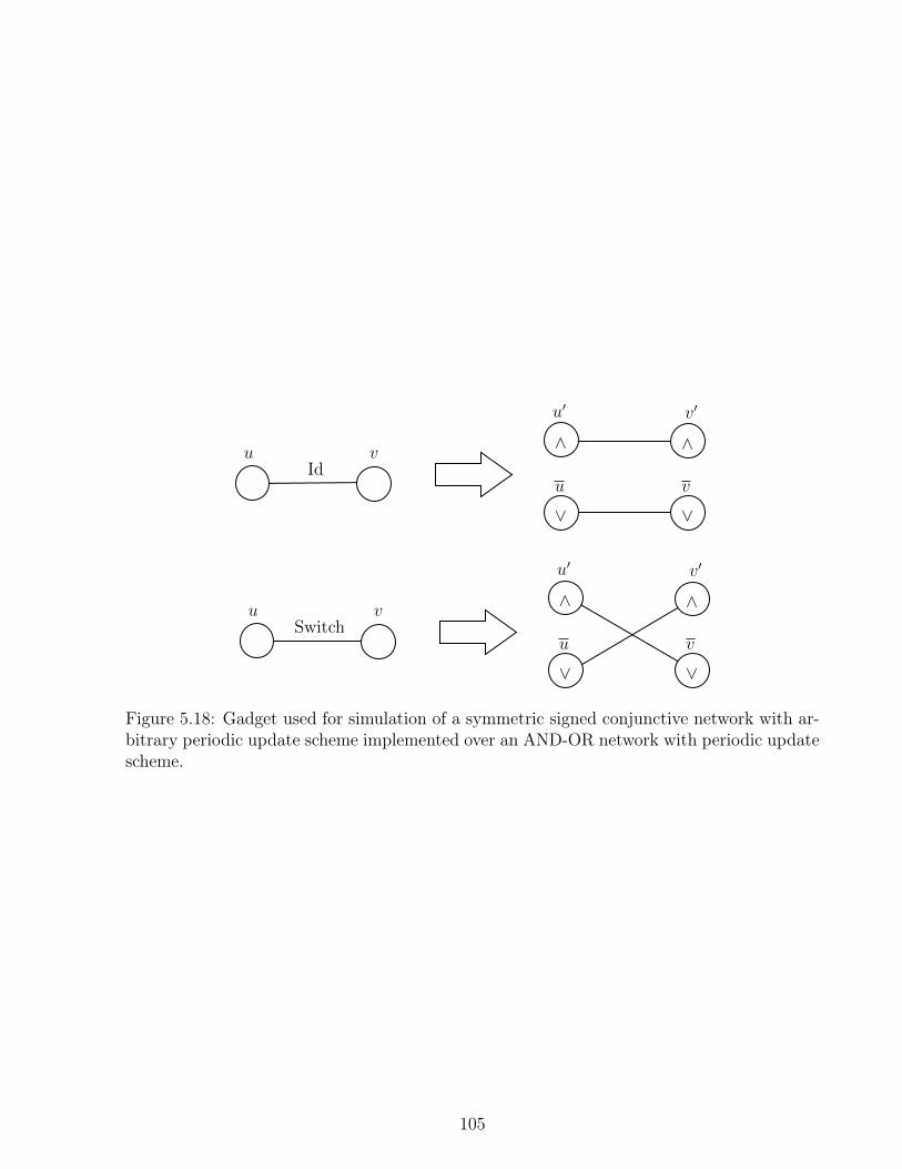
u vId

u0

u

v0

v

^^

__v

v0

u

u0

Switchvu

Figure 5.18: Gadget used for simulation of a symmetric signed conjunctive network with ar-bitrary periodic update scheme implemented over an AND-OR network with periodic updatescheme.

105

Chapter 6

Freezing dynamics

The main aim of this section is to study the dynamics of freezing automata networks.Roughly, a freezing automata network is an automata network in which the alphabet isequipped with a partial order and the global function is non-decreasing for this order. Thissection is organized in two subsections:

1. in the first subsection a general framework that captures several classical dynamicaldecision problems is defined. In particular, this task is accomplished by introduc-ing a model checking problem called SPEC, which asks for the existence of an orbitof a freezing automata network that satisfies certain local constraints in the trace ofeach node. In addition, a set of three main parameters are identified, grouped in twocategories: interaction graph parameters (maximum degree and treewidth of interac-tion graph) and the alphabet size. In this context, a fast parallel algorithm to solvegeneral SPEC problem is presented. Then, it is shown that latter decision problem,when parametrized using the previous parameter set is not fixed parameter tractableW[2] = FPT (which is considered unlikely). Finally, the effect of treewidth param-eter is studied by considering latter problem restricted to families of sufficiently largetreewidth. More precisely, it is shown that in this context latter classical dynamicaldecision problems are complete in their respective classes.

2. The second subsection goes further in the study of non-deterministic freezing automatanetworks by considering a disease spread model based in the well-known Bootsrap Per-colation model. We particularly address the problem of computing the probability ofcontagion for some fixed node in the network, and evaluate how the network topol-ogy impacts the computational complexity of the latter task (addressed as a countingproblem). In this context, the previous problem is seen as a counting version of theprediction problem. Thus, a parallel between it and previous results on the predictionproblem in the context of this model is proposed.

106

6.1 Specification checking problem: a canonical modelchecking problem to capture many classical dynami-cal problems.

The present subsection aims at understanding what are the key parameters which influencethe overall computational complexity of finite freezing automata networks. A natural firstparameter is the alphabet size, since automata networks are usually considered as simplemachines having a number of states that is independent of the size of the network. Inaddition, in the case of freezing dynamics, the alphabet is also a bound for the number ofchanges that some node can exhibit in an arbitrary orbit. For the same reasons, a secondparameter that we consider is the maximum degree of the network, as a simple machinemight not be able to handle the information incoming from a large number of neighbors.The last parameter is inspired by the results which show some computational limitationsbetween freezing automata networks defined over bi-dimensional grids and one-dimensionalgrids [66, 46, 77] (i.e. paths or rings). Since Courcelle’s theorem on MSO properties [17],graph parameters like treewidth [71] are used to measure a sort of distance to a tree graphand indirectly an indication of the largest grid minor structure. Indeed, it is known thatpaths or rings have constant treewidth, and the treewidth of a graph is polynomially relatedto the size of its largest grid minor [16]. Therefore treewidth is a natural parameter for ourstudy.

The present subsection is divided in several subparts organized as follows:

Localized trace properties. We define a general model checking problem, called SPEC, thatasks whether a given freezing automata network has an orbit that satisfies a given set of localconstraints on the trace at each node (Problem 6.1.1). It takes advantage of the sparse orbitsof freezing automata networks (a bounded number of changes per node in any orbit) whichallow to express properties in the temporal dimension in an efficient way. We show thanks toa kind of pumping lemma on orbits (Lemma 6.2) that it captures many standard problemsin automata network theory, among which we consider four ones: prediction [33, 31, 46],nilpotency [70, 27, 51], predecessor [52, 45] and asynchronous reachability [21]. Note thatsince Boolean circuits are easily embedded into freezing automata networks, our frameworkalso includes classical problems on circuit: circuit value problem is a sub-problem of ourprediction problem (see Theorem 6.21) and SAT is a sub-problem of our nilpotency problem(see Remark 6.4 and Theorem 6.19).

Fast parallel algorithm. We present a NC algorithm that solves our general model checkingproblem SPEC on any freezing automata network with bounded number of states and graphwith bounded degree and bounded treewidth (Theorem 6.13). It solves in particular the fourcanonical problems above in NC for such graphs, as well as circuit value problem and SAT(see [73, 11] for better known results for these specific problems). Note that our algorithmis uniform in the sense that, besides the graph, both the automata network rule and theconstraint to test are part of the input and not hidden in an expensive pre-processing step.As suggested above, temporal traces of the evolution of a bounded set of nodes have a spaceefficient representation. However, it is generally hard to distinguish real orbits projected ona set of nodes from locally valid sequences of states that respect the transition rule for these

107

nodes. Our algorithm exploits bounded treewidth and bounded degree to solve this problemvia dynamic programming for any finite set of nodes. In the deterministic case, our algorithmcan completely reconstruct the orbit from the initial configuration.

Hardness results. In light of Courcelle’s theorem, one might think that our algorithm solv-ing SPEC could be directly obtained (or even improved) by simply expressing the problem inMSOL (monadic second order logic) [17]. We show that it is impossible, unless W[2] = FPT

(which is unlikely). More precisely, we show that the version of our model checking problemwhere treewidth is the unique parameter and alphabet and degree are fixed is W[2]-hard(Corollary 6.16), and thus it is not believed to be fixed parameter tractable. We obtain asimilar result on a slight variation of our problem when the alphabet is the unique parameterand treewidth and degree are fixed (Corollary 6.17). In addition, one might also interpretSPEC as a particular instance of the Constraint Satisfaction Problem (CSP) which consistsin some sort of generalization of SAT that considers a more versatile variable constraints.However, as we remark in the next sections, this approach does not provide any improvementscompared to our algorithm.

Finally, we show that the four problems mentioned before, (namely prediction, nilpotency,predecessor and asynchronous reachability) are complete in their respective class (respec-tively P-complete and coNP-complete for the first two, and NP-complete for the last one)when we restrict the input graphs to a constructible family of sufficiently large treewidth(Theorems 6.19, 6.20 and 6.21). To do so, we depend on an efficient algorithm to embed ar-bitrary (but polynomially smaller) digraph into our input graph (Lemma 6.18), which relieson polynomial perfect brambles that can be efficiently found in graphs with polynomiallylarge treewidth [55] (here by polynomial we mean ⌦(n↵

) for some positive real number ↵).This embedding allows to simulate a precise dynamics on the desired digraph inside the inputgraph and essentially lifts us from the graph family constraint as soon as the treewidth is largeenough. Moreover, for problems prediction (Theorem 6.21), predecessor and asynchronousreachability (Theorem 6.20) we achieve the hardness result with a fixed uniform set-definedrule (i.e. a rule that change the state of each node depending only on the set of states seen inthe neighborhood) which is not part of the input. This shows that there is a uniform isotropicuniversally hard rule for these problems, which makes sense for applications like bootstrappercolation, epidemic propagation or cristal growth where models are generally isotropic andspatially uniform.

6.1.1 Localized Trace Properties

In this section we formalize the general decision problem we consider on our dynamical sys-tems. Freezing automata networks have temporally sparse orbits, however the set of possibleconfigurations is still exponential. Our formalism takes this into account by considering prop-erties that are spatially localized but without restriction in their temporal expressive power.More precisely, we introduce the concept of a specification.

Definition 6.1 Let t be a natural number and A = (G = (V,E), F ) a non-deterministicfreezing automata network in some partially-ordered alphabet Q. A (Q, t,A)-specification (orsimply a t-specification when the context is clear) is a function Et : V ! P(Qt

) such that,

108

for every v 2 V , the sequences in Et(v) are non-decreasing.

Pumping lemma on orbits. The following lemma shows that for all freezing automatanetworks the set of orbits of any length restricted to a set of nodes is determined by theset of orbits of fixed (polynomial) length restricted to these nodes. Moreover, if the set ofconsidered nodes is finite, then the fixed length can be chosen linear.

Lemma 6.2 Let Q be an alphabet, V a set of nodes with |V | = n and U ✓ V . Let L =

|U ||Q|(|Q|n + 1). Then if two non-deterministic freezing automata networks over QV havethe same set of orbits restricted to U of length L then they have the same set of orbitsrestricted to U of any length.

Proof. Any orbit restricted to U of any length can be seen as a sequence of elements of QU

and, since the considered automata network is freezing, there are at most |U ||Q| changes inthis sequence so that it can be written pt1

1pt22· · · ptmm with m |U ||Q|, pi 2 QU and ti 2 N. The

key observation is that pt11pt22· · · pti�1

i�1p|Q|n+1

ipti+1

i+1· · · ptmm is a valid restricted orbit if and only

if pt11pt22· · · pti�1

i�1pTipti+1

i+1· · · ptmm is a valid restricted orbit for all T � |Q|n+ 1: this is because

any sequence of |Q|n+ 1 configurations in any orbit must contain two consecutive identicalconfigurations since |Q|n is the maximal total number of possible state changes. From thiswe deduce that it is sufficient to know all the restricted orbits of the form pt1

1pt22· · · ptmm

with ti |Q|n+ 1 and m |U ||Q| to know all restricted orbits of any length. The lemmafollows.

Note that as a consequence of the last lemma, for any freezing non-deterministic automatanetwork it suffices to consider t-specifications with t being linear in the size of the interactiongraph defining the network.

Specification checking problem.

We observe that the number of possible t-specifications can be represented in polynomialspace in the size of the network (as a Boolean vector indicating the allowed t-specifications).Also, in the absence of explicit mention, all the considered graphs will have bounded degree� by default, so a freezing automata network rule can be represented as the list of localupdate rules for each node which are maps of the form Q� ! P(Q) whose representation asa transition table is of size O

�|Q|�+1

�.

The specification checking problem we consider asks whether a given freezing automatanetwork verifies a given localized trace property on the set of orbits whose restriction on eachnode adheres to a given t-specification. To this end, we introduce the concept of a satisfiablet-specification.

Definition 6.3 Let A = (G,F ) be a non-deterministic automata network and let Et a t-specification. We say that Et is satisfiable by A if there exists an orbit O 2 O(A, t) such thatOv 2 Et(v) for every v 2 V.

109

If Et is a satisfiable t-specification for some automata network A we write A |= Et. Wepresent now the Specification checking problem as the problem of verifying whether a givent-specification is satisfiable by some automata network A.

Problem (Specification checking problem (SPEC))

Parameters: alphabet Q, family of graphs G of max degree �.

Input:

1. a non-deterministic freezing automata network A = (G,F ) on alphabet Q, withset of nodes V and G 2 G;

2. a time t 2 N.3. a t-specification Et

Question: A |= Et?

We remark that it could be also possible to present some sort of universal version of thelast problem, in which we could ask not only if the given t-specification Et is satisfiable inthe sense of checking for the existence of some orbit of the system verifying some propertycoded in Et but checking if every orbit verifies the latter property.

Four canonical problems.

When studying a dynamical system, one is often interested in determining properties of thefuture state of the system given its initial state. In the context of deterministic automatanetworks, various decision problems have been studied where a question about the evolu-tion of the dynamics at a given node is asked. Usually, the computational complexity ofsuch problems is compared to the complexity of simulating step by step the automata net-work. Roughly speaking, one can observe that some systems are complex in some way if thecomplexity of latter problems are “as hard" as simply simulating the system.

Problem (Prediction problem)

Parameters: alphabet Q, family of graphs G of max degree �

Input:

1. a deterministic freezing automata network A = (G,F ) on alphabet Q, with set ofnodes V with n = |V | and G 2 G;

2. an initial configuration c 2 Qn;3. a node v 2 V and a time t 2 N;4. A t-specification Et satisfying: for all y 2 Et(v), y0 = cv.

Question: A |= Et

110

Note that this prediction problem is clearly a subproblem of SPEC. Also, observe thata specification allows us to address various questions considered in the literature: what willbe the state of the node at a given time [31, 46], will the node change its state duringthe evolution [33, 35, 34], or, thanks to Lemma 6.2, what will be state of the node oncea fixed point is reached [66, Section 5]. Note that the classical circuit value problem forBoolean circuits easily reduces to the prediction problem above when we take G to be theDAG of the Boolean circuit and choose local rules at each node that implement circuit gates.Theorem 6.21 below gives a much stronger result using such a reduction where the graphand the rule are independent of the circuit.

Now we turn to the classical problem (in the context of deterministic automata networks)of finding predecessors back in time to a given configuration [52, 44].

Problem (Predecessor Problem)

Parameters: alphabet Q, family of graphs G of max degree �

Input:

1. a deterministic freezing automata network A = (G,F ) on alphabet Q, with set ofnodes V with n = |V | and G 2 G ;

2. a configuration c 2 QV

3. a time t 2 N

Question: 9y 2 QV: F t

(y) = c?

Note that, analogously to the previous case, the final configuration in the input can begiven through a particular t-specification Et, such that for all y 2 Et(v) : yt = c for any v 2 V .Thus, by considering Et we can see predecessor problem as a subproblem of SPEC.

Deterministic automata networks have ultimately periodic orbits. When they are freezing,any configuration reaches a fixed point. Nilpotency asks whether their is a unique fixed pointwhose basin of attraction is the set of all configurations. It is a fundamental problem in finiteautomata networks theory [70, 27] as well as in cellular automata theory where the problemis undecidable for any space dimension [51], but whose decidability depends on the spacedimension in the freezing case [66].

Problem (Nilpotency problem)

Parameters: alphabet Q, family of graphs G of max degree �

Input: a deterministic freezing automata network A = (G,F ) on alphabet Q, with set ofnodes V and G 2 G;

Question: is there t � 1 such that F t(QV

) is a singleton?

111

In this case, it is not clear that Nilpotency is actually a subproblem of SPEC. However, wewill show that we can solve Nilpotency by solving a polynomial amount of instances (linearon the size of the interaction graph of the network |G|) of SPEC in parallel. More precisely,we show that there exist a NC Turing reduction of NIL to SPEC. In order to do that, first,note that we can use Lemma 6.2 to fix t = �(n), where �(n) is an appropriate polynomial.Then, we express that F �(n)

(QV) is a singleton as the following formula, which intuitively

says that for each node there is a state such that all orbits terminate in that state at thisnode:

Vs2V

Wq02Q A |= Eq0,s

�(n), where Eq0,s�(n) are �(n)-specifications satisfying Eq0,s

�(n)(v) = Qt, forevery v 6= s and Eq0,s

�(n)(s) is the set of orbits y such that y�(n) = q0. The reduction holds.

It is straightforward to reduce coloring problems (does the graph admit a proper coloringwith colors in Q) and more generally tilings problems to nilpotency using an error state thatspread across the network when a local condition is not satisfied (note that tiling problemare known to be tightly related to nilpotency in cellular automata [51]). Using the sameidea one can reduce SAT to nilpotency by choosing G to be the DAG of a circuit computingthe given SAT formula (see Theorem 6.19 below for a stronger reduction that works on anyfamily of graphs with polynomial treewidth).

Remark 6.4 If we allow the input automata network to be associated to a graph of un-bounded degree (the local rule is then given as a circuit), it is possible to reduce any SATinstance to an automata network on a star graph with alphabet Q = {0, 1, "} where the cen-tral node simply checks that the Boolean values on leafs represent a satisfying instance ofthe SAT formula and produces a " state that spreads over the network if it is not the case.The circuit representing the update rule of each node is NC in this case, and the automatanetwork is nilpotent if and only if the formula is not satisfiable.

Given a deterministic freezing automata network of global rule F : QV ! QV , we definethe associated non-deterministic global rule F ⇤ where each node can at each step to applyF or to stay unchanged, formally: F ⇤

v (c) = {Fv(c), cv}. It represents the system F undertotally asynchronous update mode.

Problem (Asynchronous reachability Problem)

Parameters: alphabet Q, family of graphs G of max degree �

Input:

1. a deterministic freezing automata network A = (G,F ) on alphabet Q, with set ofnodes V with n = |V | and G 2 G;

2. an initial configuration c0 2 QV

3. a final configuration c1 2 QV

Question: can c1 be reached starting from c0 under F ⇤?

Note that no bound is given in the problem for the time needed to reach the target

112

configuration. However, Lemma 6.2 ensures that c1 can be reached from c0 if and only if itcan be reach in a polynomial number of steps (in n). Thus this problem can be reduced toSPEC by defining a �(n)-specification E�(n) such that for any y 2 E�(n) : y0 = c0 ^ y�(n) = c1.This bound on the maximum time needed to reach the target ensures that the problem isNP (a witness of reachability is an orbit of polynomial length). Note that the problem isPSPACE-complete for general automata networks: in fact it is PSPACE-complete even whenthe networks considered are one-dimensional (network is a ring) cellular automata (same localrule everywhere) [21].

6.1.2 A fast parallel algorithm for Specification Checking

In this section we present a fast-parallel algorithm for solving the Specification CheckingProblem when the input graph is restricted to the family of graphs with bounded degree andtreewidth. More precisely, we show that the problem can be solved by a CREW PRAM thatruns in time O(log

2(n)) where n is the amount of nodes of the network. Thus, restricted to

graphs of bounded degree and bounded treewidth, Specification Checking Problem belongs tothe class NC.

To explain how our main algorithm solve the latter problem, we will divide it in a numberof sub-routines, that can be executed efficiently in parallel. Then, we will present an NCalgorithm for Specification Checking problem as a combination of these sub-routines. Webegin fixing sets Q, G, and natural numbers � and k. Let A = (G,F), t and Et be aninstance of the Specification Checking Problem, that we consider for the following definitions.

Definition 6.5 A locally-valid trace of a node v 2 V is a function ↵ : N [v]! Qt such that:

1. ↵(v)s+1 2 Fv((↵(u)s)u2N [v]) for all 0 s < t,2. ↵(v) belongs to Et(v).

We call the set of all locally-valid traces of v as LV T (v)

Intuitively, a locally-valid trace of a vertex v is a sequence of state-transitions of all thevertices in N [v] which are consistent with the local rule of v, but not necessarily consistentwith the local rules of the vertices in N(v). We also ask that the state-transitions of v satisfythe specification E .

Given two finite sets A,B, and a function f : A! B. We define the restriction functionof f to a subset A0 ✓ A as the function f |0A : A0 ! B such that, for all v 2 A0 we have thatf |0A(v) = f(v).

Definition 6.6 Let U ✓ V be a subset of nodes. A partially-valid trace of a set of nodesU ✓ V is a function � : N [U ]! Qt such that �|N [v] belongs to LV T (v) for each v 2 U .

We call the set of all partially-valid traces of U as PV T (U).

Roughly, a partially-valid trace for a set U is a sequence of state-transitions of all the

113

vertices in N [U ], which are consistent with the local rules of all vertices in U , but notnecessarily consistent with the local-rules of the vertices in N(U).

Let (W,F, {Xw : w 2 W}) be a rooted binary-tree-decomposition of the graph G withroot r, that we assume of width at most (3 tw(G) + 2). For w 2 W , we call Tw the set of allthe descendants of w, including w.

Our algorithm consists in a dynamic programming scheme over the bags of the tree.First, we assume that PV T (Xw) is nonempty for all bags w 2 W , otherwise the answer ofthe Specification Checking problem is false. For each bag w 2 T and �w 2 PV T (Xw) we callSolw(�w

) the partial answer of the problem on the vertices contained bags in Tw, when thelocally-valid traces of the vertices in Xw are induced by �w. We say that Solw(�w

) = accept

when it is possible to extend �w into a partially-valid trace of all the vertices in bags of Tw,and reject otherwise. More precisely, if w is a leaf of T , we define Solw(�w

) = accept forall �w 2 PV T (Xw). For the other bags, Solw(�w

) = accept if and only if there exists a� 2 PV T (

Sz2Tw

Xz) such that �(u) = �w(u), for all u 2 Xw. Observe that the instance of

the Specification Checking problem is accepted when there exists a �r 2 PV T (Xr) such thatSolr(�r

) = accept where r is the root of the tree. The following lemma is the core of ourdynamic programming scheme:

Lemma 6.7 Let w be a bag of T that is not a leaf and �w 2 PV T (Xw). Then Solw(�w) =

accept if and only if for each child v of w in Tw there exists a �v 2 PV T (Xv) such that

1. �w(u) = �v

(u) for all u 2 N [Xw] \N [Xv],2. Solv(�v

) = accept

Proof. First, let us assume that Solw(�w) = True and let v be one of the children of w

in Tw. This implies that there exists a partially-valid trace � 2 PV T (S

z2TwXz) such that

�(u) = �w(u), for all u 2 Xw. Observe that N [[z2Tv

Xz] ✓ N [(S

z2TwXz]. Since � is

defined over N [(S

z2TwXz], we can define �v and �Tv as the restrictions of � to the sets

N [Xv] and N [[z2TvXz], respectively. Observe that �v satisfies the condition (1) and (2)

because, by definition, �v(u) and �w

(u) are both equal to �(u) for all u 2 N [Xw] \ N [Xv].Moreover, SolwL

(�v) = accept because �Tv is a partially-valid trace of

Sz2Tv

Xz such that�v

(u) = �(u) = �Tv(u) for each u 2 Xv.

Conversely, suppose that we have that conditions (1), (2) for each child of w. If w is a leafthe proposition is trivially true. Suppose then that w is not a leaf. For each child v of w, let�v be the partially-valid trace of Xv satisfying that Solv(�v

) = accept and �v(u) = �w

(u)for each u 2 N [Xw]\N [Xv]. Since Solv(�v

) = accept we know that �v can be extended intoa partially-valid trace of [z2Tv

Xz, that we call �Tv . Let us call v1 and v2 the children of w.We define then the function � : N [[z2Tw

Xz]! Qt.

�(u) =

8<

:

�w(u) if u 2 N [Xw]

�Tv1 (u) if u 2 N [S

z2Tv1Xz]

�Tv2 (u) if u 2 N [S

z2Tv2Xz]

114

We claim that there is no ambiguity in the definition of �. First, we claim that N [S

z2Tv1Xv]\

N [S

z2Tv2Xv] is contained in N [Xu]. Indeed, let u be a vertex in N [

Sz2Tv1

Xz]\N [S

z2Tv2Xz].

There are three possibilities:

• u belongs to a bag in Tv1 and to another bag in Tv2 . In this case necessarily u 2 Xw,because otherwise the bags containing u would not induce a (connected) subtree of T .

• u is not contained in a bag of Tv1 . Since u belongs to N [S

z2Tv1Xz], there exists a

vertex u adjacent to u and contained in a bag of Tv1 . Note that Xw contains u, becauseotherwise all the bags containing u would be in Tv1 . Then, no bag would contain both uand u. That contradicts the property of a tree-decomposition that states that for eachedge of the graph G, there must exist a bag containing both endpoints. We deduce uis contained in Xw and then u is contained in N [Xw].

• u is not contained in a bag of Tv2 . This case is analogous to the previous one.

Following an analogous argument, we deduce that N [S

z2Tv1Xz] \ N [Xw] is contained in

N [Xv1 ] and that N [S

z2Tv2Xz] \ N [Xw] is contained in N [Xv2 ]. We deduce that � is well

defined. Moreover, � is a partially-valid trace ofS

z2TwXz which restricted to N [Xw] equals

�w. We conclude that Solw(�w) = accept.

In order to solve our problem efficiently in parallel, we define a data structure that allowsus to efficiently encode locally-valid traces and partially-valid traces. More precisely, in N [v]there are at most |Q|� possible state transitions. Therefore, when t is comparable to n, mostof the time the vertices in N [v] remain in the same state. Then, in order to efficiently encodea trace, it is enough to keep track only of the time-steps on which some state-transitionoccurs.

Let U be a set of vertices of G. A (U, t)-sequence S is a function S : U ! Qt such that thesequence S(u) is non-decreasing, for all u 2 U . For each 0 s t let us call Ss the sequence(S(u)s)u2U 2 |Q||U |. Let Times(S) = (t0, t1, . . . , t`) be the strictly increasing sequence ofminimum length satisfying that Sti = Ss for each ti s < ti+1 and each 0 i < `. Observethat t0 = 0 and ` = `(S) |Q||U |. For natural numbers m and `, let us call hmi` the binaryrepresentation of m using ` bits, padded with `� dlogme zeros when ` > dlogme.

Definition 6.8 Let S be a (U, t)-sequence. A succinct representation of S, denoted "(S), isa pair (Times(S),States(S)) such that:

• Times(S) is a list of elements of {0, 1}dlog(t+1)e of length |Q||U |, such that

Times(S)i =⇢htiidlog(t+1)e if i `(S)htidlog(t+1)e if i > `(S)

• States(S) is a matrix of elements of {0, 1}dlog |Q|e of dimensions |Q||U |⇥ |U |, such that,if we call u1, . . . , u|U | the vertices of U sorted by their labels, then:

States(S)i,j =⇢hS(uj)tiidlog |Q|e if i `(S)hS(uj)tidlog |Q|e if i > `(S) .

115

We also call #(U, t) = |Q||U |dlog(t+ 1)e+ |U ||Q||U |dlog |Q|e

Observe that "(S) can be written using exactly N = #(U, t) bits. In other words, thesuccinct representations of all (U, t)-sequences can be stored in the same number of bits,which is O(|U | log t). Therefore, there are at most 2

N= tg(|U |) possible (U, t)-sequences, for

some function g exponential in |U |. Moreover, we identify the succinct representation of(U, t)-sequence S with a number x 2 {0 . . . , 2N}, such that "(S) = hxiN .

The restriction of Et to the nodes in U is denoted Et(U). When U = {u} we denote Et({u})simply Et(u).

Definition 6.9 Let U be a set of vertices an let us call N = #(U, t). A succinct represen-tation of a Et(U) is a Boolean vector X = "(Et(U)) of length 2

N such that Xi = True when i

represents the succinct representation of a (U, t)-sequence contained in Et(U).

Next lemma states that the succinct representation of a (U, t)-specification can be com-puted by a fast parallel algorithm.

Lemma 6.10 For each set of vertices U , there exist a function f and CREW PRAM algo-rithms performing the following tasks in time f(|U ||Q|) log n using nf(|U ||Q|) processors:

• Given a (U, t)-sequence S as a t⇥ |U | table of states in Q, compute "(S)• Given a Et(U) as a list of (U, t)-sequences, compute "(Et(U))

Proof.

• The algorithm first computes Times(S). Then, it constructs the list Times(S) and thematrix States(S) copying the lines of S given in Times(S).The algorithm starts reserving N = #(U, t) bits of memory for the list Times and thematrix States, and t+ 1 bits of memory represented in a vector called indices. Thevector indicess stores the time-steps on which states have changed. This informationis contained in Times(S).For each i 2 {1, . . . , t} the algorithm initializes a processor Pi and assigns the i-th bitof indices to it. Processor Pi looks at the i-th and i � 1-th lines of S. If Si 6= Si�1

then processor writes a 1 in indicesi. Otherwise, the processor writes a 0 in indicesi.Then Pi stops. All this process can be done in time O(|U | log |Q|+log t) per processor.Then, the algorithm computes the vector p of length t such that pj =

Pi

j=1indicesj,

for each j 2 {1, . . . , t}. This process can be done in time O(log t) using O(t) proces-sors using the prefix sum algorithm given by [50] (Proposition 1.19). Observe that ifindicesi = 1 for some index i, then i = Times(S)pi . Moreover, pt = `(S).Once every processor (Pi)0<it stops, the algorithms reinitialize them. For each 0 <i t, each processor Pi looks at indicesi. If pi < pt and indicesi = 0 then processorPi stops. If pi = pi�1 = pt the processor stops. If pi 6= pt and indicesi = 1, then thealgorithm writes hiidlog(t+1)e in Timespi , and for each u 2 {1, . . . , |U |} writes hSi,uidlog |Q|ein Statespi,u. If pi = pt and pi�1 6= pi, then the processor Pi writes htidlog(t+1)e in

116

Timesj and writes hSt,uidlog |Q|e in Statesj,u for each pi j |Q||U | and for eachu 2 {1, . . . , |U |}. The algorithm writes Times0 = h0idlog(t+1)e and writes hS0,uidlog |Q|e inStatesj,u for each u 2 {1, . . . , |U |}. All this process can be done in time O(|Q||U |

log t)per processor.The algorithm returns "(S) = (Times,States). The whole process takes timeO(|Q||U |

log t) and O(t) processors.• The algorithm initializes X = "(Et(U)) as 2

N bits of memory bits, all in 0. Then,it assigns one processor PS to each (U, t)-sequence S in Et(U). For each S 2 Et(U),processor PS uses the previous algorithm to compute y = "(S). Then processor PSwrites Xy = 1. Once every processor has finished, the algorithm returns X . The wholeprocess takes time O(log |X ||Q||U |

log t) and uses |X |tO(1)= nO(|Q||U|

) processors. Wededuce that the algorithm runs in time O(|Q||U |

log t) using 2N processors.

Observe that if � is a partially-valid trace of U , then in particular � is a (N [U ], t)-sequence.Therefore, there exists an x 2

N with N = #(N [U ], t), such that "(�) = x. In the followinglemma we show how to characterize the values on x 2

N that are the encoding of somepartially-valid trace of U . We need the following definition. Let U be a set of vertices andlet x 2 {0, . . . , 2N}, with N = #(U, t). Then we call Times(x) and States(x) the vectorand matrix such that x = (Times(x),States(x)). More precisely:

• Times(x) are the first |Q||U | bits of x interpreted as sequence of elements of {0, 1}dlog(t+1)e

of length |Q||U |.• States(x) are the rest of the bits of x interpreted as the matrix of elements of{0, 1}dlog |Q|e of dimensions |Q||U | ⇥ |U |.

Lemma 6.11 Let S be a (U, t)-sequence and Z ✓ U . There is a sequential algorithm whichgiven "(S) computes "(S|Z) in time linear in the size of "(S).

Proof. Let = |Q|. The computes algorithm "(S|Z) checking each pair of lines of Statesand verifying if the columns of Z differ on any coordinate, keeping only the lines on whichsome of the vertices in Z switches states for the first time. More precisely, let u1, . . . , u bethe set U ordered by their labels. Let J 2 {j1, . . . , j|Z|} be the set of indices of vertices of Z(i.e., ujq 2 Z for all q 2 {1, . . . , |Z|}). The algorithm computes the set L of indices i |Q|such that i 2 L if and only if there exists q 2 J such that Statesi,jq 6= Statesi�1,jq . Let{i1, . . . , i|L|} the indices in L. Observe that |L| |Q||Z|. Then for each p |Q||Z| and q 2 |Z|,

Times[Z]p =⇢

Timesip if p |L|htidlog(t+1)e if i > |L|

States[Z]p,q =⇢

Statesip,jq if p |L|Statest,jq if p > |L| .

117

The algorithm returns (Times[Z],States[Z]).

Lemma 6.12 Let U be a set of vertices and let N = #(N [U ], t). There is a sequential algo-rithm which, given x � 0 and "(Et(u)) for each u 2 V (G), decides in time f(|N [U ]||Q|) log nwhether x is a succinct representation of a partially-valid trace of U , where f is an exponentialfunction.

Proof. Let U be a set of vertices containing S and let x 2 {0, . . . , 2N}, with N = #(N [U ], t).Let = |N [U ]|. Let {u1, . . . , u} be the vertices of N [U ] ordered by label. The algo-rithm first verifies that x 2

N and rejects otherwise. Then, the algorithm verifies thatthe pair (Times,States) = (Times(x),States(x)) satisfies Times0 = 0 and that Timesand each column of States are increasing. Otherwise, the algorithm rejects because x isnot a succinct representation of a (N [U ], t)-sequence. If the algorithm passes this test weassume that x = "(S) for some (N [U ], t)-sequence S. For a subset of vertices Z, let us call(Times[Z],States[Z]) = "(S|Z). Consider now the following conditions:

1. Statesi,j 2 Fuj(States[N [uj])]i) for each i 2 {0, . . . , |Q|} and j 2 {1, . . . ,} such

that uj 2 U .2. (Times[{uj}],States[{uj}]) belongs to Et(uj) for each j 2 {1, . . . ,}.

When this conditions are satisfied, we can deduce that x = "(�) for some partially-valid trace � of U . Indeed, as x is representation of S, the vertices in N [U ] only havestate-transitions of the time-steps given by the Times. Therefore, condition (1.) and (2.)imply that S|N [u] is a locally-valid trace of u. To verify condition (1.) and (2.) we usethe algorithm of Lemma 6.11 to compute States[Z] for a given set of vertices Z ✓ N [U ].Observe that the algorithm computes Times[Z] and States[Z] in time O(|Q| log n). Thealgorithm checks (1.) by looking at each row of States[N [u]] and the column correspondingto vertex u, and the table of Fu given in the input. The algorithm verifies (2.) computing"(S(uj)) = (Times[{uj}],States[{uj}]) and then looking at the "(S(uj))-element of thetable "(Et(uj)). All these processes take time O(|U ||Q| log n). Overall the whole algorithmtakes time O(|U ||Q| log n) = f(|N [U ]||Q|) log n.

We are now ready to give our algorithm solving the Specification Checking problem.

Theorem 6.13 Specification Checking problem can be solved by a CREW PRAM algorithmrunning in time O(log

2 n) and using nO(1) processors on graphs of bounded treewidth.

Proof. Our algorithm consists in an implementation of the dynamic programming schemeexplained at the beginning of this section. It starts computing a rooted binary-tree decompo-sition (W,F, {Xw : w 2 W} of the input graph using the logarithmic-space algorithm givenby Proposition 1.18.

The algorithm also computes the succinct representations of E and Iv for each v 2 Vusing Lemma 6.10.

118

Then, the algorithm performs the dynamic programming scheme over T . Let r be theroot of T . Then, for a bag w 2 W , we define the level of w denoted by Level(w), as thedistance between w and the root r. There is a fast-parallel algorithm computing the level ofeach vertex of a tree by a EREW PRAM running in time O(log n) and using O(n) processors[50]. Using a prefix-sum algorithm we can compute the maximum level M of a vertex, whichcorresponds to the leafs of the binary-tree T . For each i 2 {0, . . . ,M}, let Li the set of bagsw such that Level(w) = M � i.

For each w 2 W , we represent the values of the function Solw as a table Sw indexed as atable of size 2

N , with N = O(|Q|�(3 tw(G)+2+k)log n) greater that #(N [Xw], t) for all w 2 W .

Each x 2 {0, . . . , 2N} is interpreted as a potentially succinct encoding of a partial-valid trace�. Initially Sw

= 02N , which meaning that a priori we reject all x 2 {0, . . . , 2N}. Then,

our algorithm iterates in a reverse order over the levels of the tree, starting from L0 untilreaching the the root r 2 LM . In the i-th iteration, we compute for each bag w 2 Li theset of all x 2 {0, . . . , 2N} that represent partially-valid traces �w 2 PV T (Xw) such thatSolw(�w

) = accept. To do so, the algorithm uses the calculations done on the bags in Li�1,and use Lemma 6.7. The algorithm saves the answer of each partial solution in a variableout consisting in |W | bits, such that, and the end of the algorithm out = 1

|W | if and only theinstance of the Specification Checking problem is accepted.

At the first iteration, for each w 2 L0 the algorithm sets in parallel Swx = 1 for all

x representing a partially-valid trace of w, because Solw(�w) is defined to accept for all

partially-valid trace of a leaf of T . Therefore, in parallel for all bag w 2 L0, the algorithmruns 2N parallel instances of the algorithm of Lemma 6.12, one for each x 2 {0, . . . , 2N}, andfor each one that is accepted, the algorithm writes Sw

x = 1. Once every parallel verificationfinishes, the algorithm sets outw = 1. We now detail the algorithm on the i-th iteration,assuming that we have computed Sw for all bag w 2 Li�1.

Let w be a vertex in Li and let us call wL and wR the children of w, which belong toLi�1. Roughly, as we know the partial solutions restricted to the subtrees rooted at w1

and w2, the algorithm will try to extend it to a partial solution of w according to the gluingprocedure given by Lemma 6.7, testing all possible combinations. More precisely, we initializea set of |Li| processors {Pw}w2Li , one assigned each bag in Li. Each processor Pw verifies ifoutwL

= outwR= 1, or stops and writes outw = 0. Otherwise, processor Pw initializes a set

of 2N processors, that we call {Pwz }z2{1,...,2N}, and reserves 2N bits of memory Sw 2 {0, 1}2N .

For each z 2 2N , processor Pw

z verifies if z is a succinct representation of a partially-validtrace of Xw using Lemma 6.12. If its not the case then Pw

z stops and writes a 0 in Swz .

Otherwise, processor Pwz initializes (2

N)2 processors {Pw

z,zR,zL: zR, zL 2 {1, . . . , 2N}} and

reserves 2N ⇥ 2

N bits of memory (Swz ) 2 {0, 1}N ⇥ {0, 1}N .

If SwL

zL= 0 or SwR

zR= 0 the processor Pw

z,zR,zLstops and writes a 0 in Sw

z,zR,zL. Otherwise,

the processor Pwz,zR,zL

interprets z, zR and zL as "(�wz ), "(�w

zL) and "(�w

zR), for partially-valid

traces �z, �wLand �wR

of Xw, XwLand XwR

, respectively. Which means that �wz belongs to

PV T (Xw) and SolwL(�zL) = SolwL

(�zL) = accept. Therefore �z is a partially-valid trace ofXw and �zL and �zR verify the condition (2) of Lemma 6.7. Up to this point, all verificationscan be done in time O(N) = O(|Q|�(3 tw(G)+2+k)

log n) because we are just looking at thecoordinates in the given tables.

119

Then, the processor Pwz,zL,zR

computes sets YL = N [Xw]\N [XwL] and using the algorithm

of Lemma 6.11 computes "(�w|YL) and "(�wL |YL

). If "(�w|YL) = "(�wL |YL

) the processordeduces that �w

(u) = �wL(u), for all u 2 N [Xw] \ N [XwL]. Then Pw

z,zL,zRcomputes sets

YR = N [Xw] \ N [XwR] and using the algorithm of Lemma 6.11 computes "(�w|YR

) and"(�wR |YR

). Then, if "(�w|YR) = "(�wR |YR

) the processor deduces that �w(u) = �wR(u), for all

u 2 N [Xw]\N [XwR]. If both verifications are satisfied, processor Pw

z,zR,zLstops and writes a

1 in Swz,zR,zL

. Otherwise, the processor Pwz,zR,zL

stops and writes a 0 in Swz,zR,zL

. All of theseverifications can be executed by Pw

z,zL,zRin time O(N).

Once that all processors in {Pwz,z1,z2 : zL, zR 2 {1, . . . 2N}} finished, processor Pw

z runs aprefix-sum algorithm in Sw

z , simply summing the elements of the vector to verify if someinstance was accepted. If the result is different than 0, processor Pw

z writes a 1 in Swz , and

writes a 0 otherwise. When every processor (Pwz )z2{1,...,2N} finishes, we obtain that Sw is the

table representing function Solw. Then processor Pw runs a prefix-sum algorithm on Sw toverify that there exists a partial solution for bag Xw. If the result of the prefix sum equalszero, processor Pw stops and writes a outw = 0. Otherwise, it writes outw = 1 and stops.

After all processors (Pw)w2Li have finished, the algorithm continues with the next level.

When the last level is reached, before halting processor P r decides if outw = 1 for all w 2 Wusing a prefix-sum algorithm. If the answer is affirmative the algorithm accepts the input,and otherwise rejects. On each level, the algorithm takes time O(�|Q|2�(3 tw(G)+2)

log n)and uses nO(|Q|�(3 tw(G)+2)

) processors. Proposition 1.18 provides a construction of a binary-tree-decomposition T of depth O(log n). This means that M = O(log n), and implies thatthe whole takes time O(�|Q|2�(3 tw(G)+2)

log2 n) = O(log

2 n) and nO(|Q|�(3 tw(G)+2))= nO(1)

processors. The correctness of the algorithm is given by Lemmas 6.7, 6.10, 6.11 and 6.12.

Remark 6.14 The algorithm given in the proof of Theorem 6.13 not only computes theanswer of Specification Checking problem but it also gives the coding of the orbits satisfyingspecification Et. In the case in which the freezing automata network A = (G,F ) is deter-ministic, we can say a lot more using those algorithms. Giving t and an initial conditionx 2 Qn, we are actually capable of testing any global dynamic property in NC provided thatthis property has F t

(x) as input and it is decidable in NC. In fact, note that given an initialcondition x 2 Qn, there is only one possible orbit for each node v 2 V (G). Therefore, we areable to calculate the global evolution of the system in time t starting from x.

The proof of the previous Theorem 6.13 shows that SPEC can be solved in time f(|Q|+�(G) + tw(G)) log n using nf(|Q|+�(G)+tw(G)) processors in a PRAM machine, hence in timeng(|Q|+�(G)+tw(G)) on a sequential machine, for some computable functions f and g. In otherwords, when the alphabet, the maximum degree and the tree-width of the input automatanetwork are parameters, our result shows that SPEC is in XP. In the next section, we showthat SPEC is not in FPT, unless FPT=W[2].

120

Constraint Satisfaction Problem

We remark that problem SPEC can be interpreted as a specific instance of the ConstraintSatisfaction Problem (CSP). Problem CSP is a sort of generalization of SAT into a setof more versatile variable constraint. It is formally defined as a triple (X,D,C), whereX = {X1, . . . , Xn} is a set of variables, D = {D1, . . . , Dn} is a set of domains where arepicked each variable, and a set C = {C1, . . . , Cm} of constraints, which are k-ary relationsof some set of k variables. The question is whether there exists an assignment of values toeach variables in their corresponding domains, in order to satisfy each one of the constraints.As we mentioned, SPEC can be seen as a particular instance of CSP, where we choose onevariable for each node of the input graph. The domain of each variable is the set of all locallyvalid traces of the corresponding node. Finally, we define one constraint for each node, wherethe variable involved are all the vertices in the close-neighborhood of the corresponding node,and the relation corresponds to the consistency in the information of the locally-valid tracesinvolved.

Now consider an instance of SPEC with constant tree-width, maximum degree and size ofthe alphabet, and construct the instance of CSP with the reduction described in the previousparagraph. Then, the obtained instance of CSP has polynomially-bounded domains andconstant tree-width, where the tree-width of a CSP instance is defined as the tree-width ofthe graph where each variable is a node, and two nodes are adjacent if the correspondingvariables appear in some restriction. Interestingly, it is already known that in these conditionsCSP can be solved in polynomial time [72, 18, 59] . This implies that, subject to the givenrestrictions, SPEC is solvable in polynomial time using the given algorithm for CSP as ablackbox.

The algorithm given in the proof of Theorem 6.13 is better than the use of the CSPblackbox in two senses. First, we obtain explicit dependencies on the size of the alphabet,maximum degree and tree-width. Second, the Prediction Problem is trivially solvable inpolynomial time, and then the use of the CSP blackbox gives no new information for thisproblem. Moreover, as we mentioned in Remark 6.14, our algorithm does not only decidesSPEC, but can also be used to obtain a coding of the orbit satisfying the given specification,and moreover, the possibility to test any NC property on a deterministic freezing automatanetworks.

6.1.3 W[2]-hardness results

The goal of this section is to show that, even when the alphabet and the degree are fixedand the treewidth is considered as the only parameter, the SPEC problem is W[2]-hard(see [23] for an introduction to the W hierarchy) and thus, it is not believed to be fixedparameter tractable. This is in contrast with classical results of Courcelle establishing thatmodel-checking of MSO formulas parametrized by the treewidth is fixed-parameter tractable[17] (see [54, 23] to place the result in a wider context).

Lemma 6.15 There is a fixed alphabet Q and an algorithm which, given k 2 N and a graphG of size n, produces in time O(k · nO(1)

):

121

• a deterministic freezing automata network A = (G0,F) with alphabet Q and where G0

has treewidth O(k) and degree 4

• a O(n2)-specification E

such that G admits a dominating set of size k if and only if A |= E .

The construction of the lemma works by producing a freezing automata network on aO(k)⇥ n2-grid together with a specification which intuitively work as follows. A row of thegrid is forced (by the specification) to contain the adjacency matrix of the graph, k rowsserve as selection of a subset of k nodes of G, and another row is used to check dominationof the candidate subset. The key of the construction is to use the dynamics of the networkto test that the information in each row is encoded coherently as intended, and raise an errorif not. The specification serves both as a partial initialization (graph adjacency matrix andtests launching are forced, but the choice in selection rows is free) and a check that no errorare raised by the tests.

Proof. Let G0= (V 0, E 0

) be the (k + 2)⇥ n2-grid where

V 0= {(i, j) : 0 i < n2, 1 j k + 2}; and

E 0= {{(i, j), (i± 1 mod n2, j)} : 0 i < n2, 1 j k + 2}[ {{(i, j), (i, j0)} : 0 i < n2, 1 j, j0 k + 2, |j � j0| = 1}.

Clearly G0 has a O(k) treewidth. The horizontal dimension (coordinate i in the grid) shouldbe thought as n block of size n. For each j we denote the jth row by Vj = {(i, j) : 0 i < n2}.The alphabet of the automata network is Q = {0, 1}⇥Q0 where the {0, 1} is the markercomponent and Q0 is verification component. A position is said to be marked if it has a 1 inits marker component. Vertically, the network is organized as follows.

• Rows V1 to Vk are called selection rows and they all have the same behavior: markingthe same unique position in each block, i.e. having horizontal coordinates s, s+ n,s+ 2n, . . ., s+ (n� 1)n marked for some s with 0 s < n. Intuitively the role of eachselection row is to select a node among the k nodes of the candidate dominating setand ensure that the selection information is coherently spread across the n blocs.

• Row Vk+2 is the graph row and its role is to hold the adjacency matrix of graph G laidout in a single row (bloc i contains the incidence vector of node i).

• Row Vk+1 is the domination row. Its role is to witness that there is a position i ineach bloc (possibly different from one bloc to another) where i is marked in the graphrow and also marked in at least one selection row. Said differently its role is to give acertificate that the k selected nodes in the selection rows are indeed a dominating setfor the graph encoded in the graph row.

The description by rows above gives some conditions on the marked position in the network.It should be clear that these conditions are satisfied if and only if the k selection rows representk nodes of the graph G that form a dominating set.

We now complete the description of A. In the verification component of states Q0 there isa special error state. The behavior of the automata network is to perform two tests to ensure

122

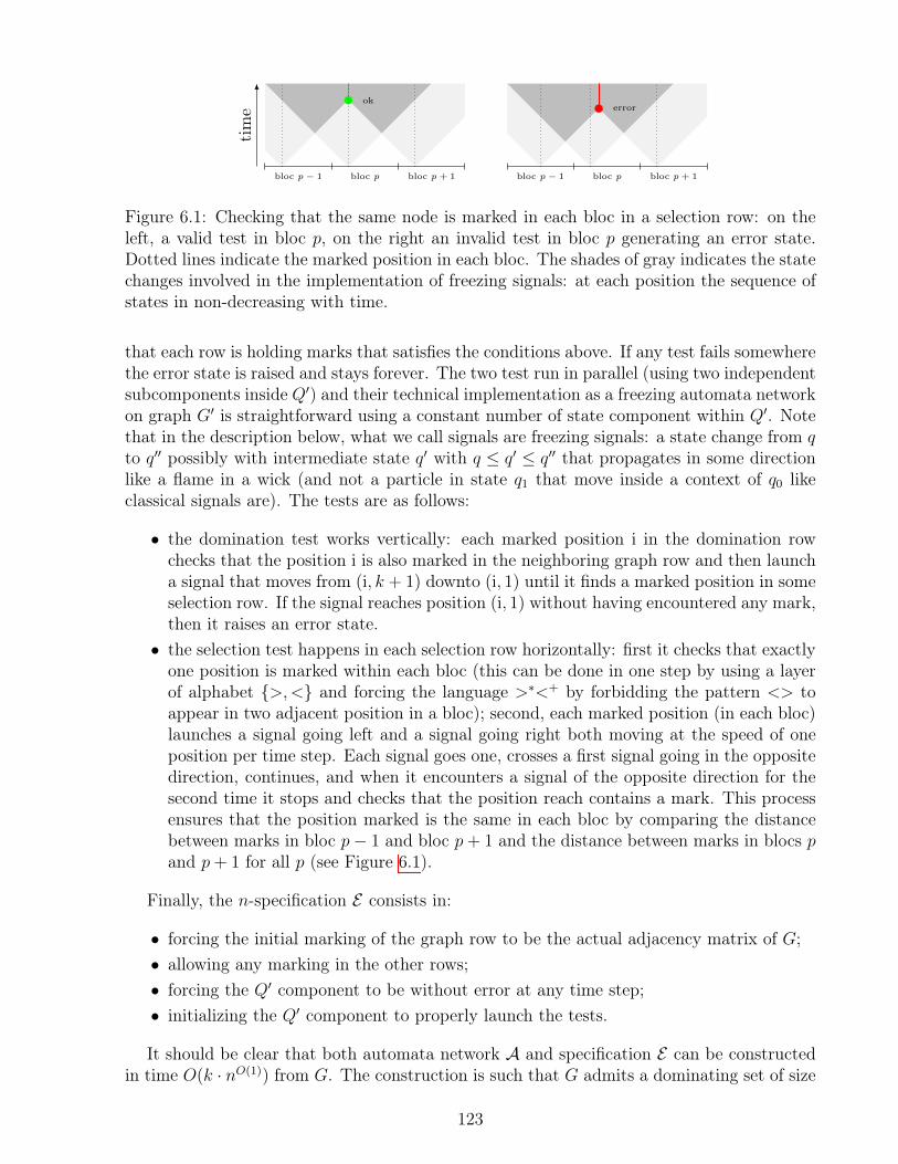
time

ok

bloc p � 1 bloc p bloc p + 1

error

bloc p � 1 bloc p bloc p + 1

Figure 6.1: Checking that the same node is marked in each bloc in a selection row: on theleft, a valid test in bloc p, on the right an invalid test in bloc p generating an error state.Dotted lines indicate the marked position in each bloc. The shades of gray indicates the statechanges involved in the implementation of freezing signals: at each position the sequence ofstates in non-decreasing with time.

that each row is holding marks that satisfies the conditions above. If any test fails somewherethe error state is raised and stays forever. The two test run in parallel (using two independentsubcomponents inside Q0) and their technical implementation as a freezing automata networkon graph G0 is straightforward using a constant number of state component within Q0. Notethat in the description below, what we call signals are freezing signals: a state change from qto q00 possibly with intermediate state q0 with q q0 q00 that propagates in some directionlike a flame in a wick (and not a particle in state q1 that move inside a context of q0 likeclassical signals are). The tests are as follows:

• the domination test works vertically: each marked position i in the domination rowchecks that the position i is also marked in the neighboring graph row and then launcha signal that moves from (i, k + 1) downto (i, 1) until it finds a marked position in someselection row. If the signal reaches position (i, 1) without having encountered any mark,then it raises an error state.

• the selection test happens in each selection row horizontally: first it checks that exactlyone position is marked within each bloc (this can be done in one step by using a layerof alphabet {>,<} and forcing the language >⇤<+ by forbidding the pattern <> toappear in two adjacent position in a bloc); second, each marked position (in each bloc)launches a signal going left and a signal going right both moving at the speed of oneposition per time step. Each signal goes one, crosses a first signal going in the oppositedirection, continues, and when it encounters a signal of the opposite direction for thesecond time it stops and checks that the position reach contains a mark. This processensures that the position marked is the same in each bloc by comparing the distancebetween marks in bloc p� 1 and bloc p+ 1 and the distance between marks in blocs pand p+ 1 for all p (see Figure 6.1).

Finally, the n-specification E consists in:

• forcing the initial marking of the graph row to be the actual adjacency matrix of G;• allowing any marking in the other rows;• forcing the Q0 component to be without error at any time step;• initializing the Q0 component to properly launch the tests.

It should be clear that both automata network A and specification E can be constructedin time O(k · nO(1)

) from G. The construction is such that G admits a dominating set of size

123

k if and only if A |= E : indeed, from the initialization imposed by E it would take at most nsteps for any of the two test to raise an error state, so E ensures that there exists an initialmarking that encodes a valid dominating set of size (at most) k as explained above.

From Lemma 6.15 and W [2]-hardness of the k-Dominating-Set problem [22], we immedi-ately get the following corollary.

Corollary 6.16 The SPEC problem with fixed degree and fixed alphabet and with treewidthas unique parameter is W[2]-hard.

A freezing automata network on a O(k)⇥ n2-grid with alphabet Q can be seen as afreezing automata network on a line of length n2 with alphabet QO(k). One might thereforewant to adapt the above result to show W[2]-hardness in the case where treewidth anddegree are fixed while alphabet is the parameter. However, the specification which is partof the input, has an exponential dependence on the alphabet (a t-specification is of sizeO(n · t|Q|

)). Therefore FPT reductions are not possible when the alphabet is the parameter.We can circumvent this problem by considering a new variant of the SPEC problem wherespecification are given in a more succinct way through regular expressions. A regular (Q, V )-specification is a map from V to regular expressions over alphabet Q. We therefore considerthe problem REGSPEC which is the same as SPEC except that the specification must bea regular specification. With this modified settings, the construction of Lemma 6.15 can beadapted to deal with the alphabet as parameter.

Corollary 6.17 The REGSPEC problem with fixed degree and fixed treewidth and withalphabet as unique parameter is W [2]-hard.

Proof. Using the construction of Lemma 6.15 and compressing the k rows into a single oneby enlarging the alphabet, we can construct a freezing automata network A↵ of alphabetQk+2 on a graph G00

= (V 00, E 00) which is a cycle of length n2 (therefore of constant treewidth

and constant degree) and that has the same behaviour with respect to k-dominating setsof the graph G of the lemma. The local map at each node of A↵ can be described by atransition table of size O(Q3k

) so the global description is of size O(Q3k · n2). Noting that

the specification produced in Lemma 6.15 is actually a regular specification of the form:v 2 V 0 7! Qi,vQ⇤

e,v where Qi,v take care of the initialization and Qe,v is the subset of stateswith no error. We deduce that the corresponding regular specification for A↵ is of the formv 2 V 00 7!

�Qi,v1 ⇥ · · ·⇥Qi,vk+2

��Qe,v1 ⇥ · · ·⇥Qe,vk+2

�⇤. Hence its size is O(|Q|O(k) · n2). The

total size of the input produced for problem REGSPEC is therefore also O(|Q|O(k) · n2) and

it can be produced in time O(|Q|O(k) · nO(1)). This proves that the k-dominating set problem

can be FPT reduced to REGSPEC with alphabet as parameter.

6.1.4 Hardness results for polynomial treewidth networks

We say a family of graphs G has polynomial treewidth if the graphs of the family are of size atmost polynomial in their treewidth, precisely: if there is a non-constant polynomial map pG

124

(with rational exponents in (0, 1)) such that for any G = (V,E) 2 G it holds tw(G) � pG(|V |).Moreover, we say the family is constructible if there is a polynomial time algorithm thatgiven n produces a connex graph Gn 2 G with n nodes. The following lemma is based ona polynomial time algorithm to find large perfect brambles in graphs [55]. This structureallows to embed any digraph in an input graph with sufficiently large treewidth via pathrouting while controlling the maximum number of intersections per node of the set of paths.

Lemma 6.18 (Subgraph routing lemma) For any family G of graphs with polynomial treewidth,there is a polynomial map p and a deterministic polynomial time algorithm that, given anygraph G = (V,E) 2 G and any digraph D = (V 0, E 0

) of maximum (in/out) degree � and sizeat most p(|V |), outputs:

• a mapping µ : V 0 ! V such that, for each v 2 V , µ�1(v) contains at most two elements,

• a collection C = (pe0)e02E0 of paths connecting µ(v01) to µ(v0

2) for each (v0

1, v0

2) 2 E 0, and

such that any node in V belongs to at most 4� paths from C.

Proof. By [55, Theorem 5.3] there exists a polynomial map p1 and a polynomial time al-gorithm that given a graph G = (V,E) 2 G finds a perfect bramble B = (B1, . . . , Bk) withk � p1(pG(|V |)), i.e. a list of connected subgraphs Bi ✓ V such that:

1. Bi \ Bj 6= ; for all i and j,2. for all v 2 V there are at most two elements of B that contain v.

We set the polynomial map of the lemma to be p = p1 � pG and consider any digraphD = (V 0, E 0

) of maximum (in/out) degree � and size at most p(|V |). We suppose k = |V 0|(by forgetting some elements of B) and reindex the element of B by V 0. The map µ : V 0 ! Vis constructed by picking some element µ(v0) 2 Bv0 for all v0 2 V 0. The fact that any vertexv 2 V is contained in at most two elements of the bramble B ensures the first condition of thelemma on µ. Now, for each (v0

1, v0

2) 2 E 0 we define a path from µ(v0

1) to µ(v0

2) as follows: let

v 2 Bv01\ Bv02

(first property of perfect brambles) then choose a path from µ(v01) to v inside

Bv01(which is connected) followed by a path from v to µ(v0

2) inside Bv02

. The collection ofpaths C thus defined is such that there are at most 2� paths that start or end in µ(v0) forany v0 2 E. Moreover, for any v 2 V , there are at most two elements of B that contain v,let’s say Bv01

and Bv02. Then the only paths from C that can go through v are those starting

or ending at either µ(v01) or µ(v0

2), so they are at most 4� in total.

Theorem 6.19 For any family G of constructible graphs of polynomial treewidth, the problemnilpotency is coNP-complete.

Proof. First, by Lemma 6.2, a freezing automata networks with n nodes is nilpotent if andonly if F �(n) is constant where �(n) 2 O(n) is the concrete computable bound from thelemma. The nilpotency problem is therefore clearly coNP.

We now describe a reduction from problem SAT. Given a formula with n variables seenas a Boolean circuit of maximum input/output degree 2 (of size polynomial in n), we first

125

construct G = (V,E) 2 G such that the DAG G0= (V 0, E 0

) associated to the circuit is of sizeat most p(|V |) where p is the polynomial map of Lemma 6.18. Then, using Lemma 6.18, wehave a map µ : V 0 ! V and a collection C of paths in G that represent an embedding of G0

inside G. The lemma gives a bound 8 on the number of paths visiting a given node v 2 V .Then each node will hold 8 Boolean values, each one corresponding either a node v0 2 V 0 ofthe Boolean circuit or an intermediate node of a path from the collection C. The alphabetis then Q = {0, 1}8 [ {?} where ? is a special error state. In any configuration c 2 QV , anode can be either in error state ?, or it holds 8 Boolean components. We then constructthe local rule at each node v 2 V that give a precise fixed role to each such component: iteither represent a node v0 2 V 0 such that µ(v0) = v, or an intermediate node in one of thepaths from C, or is unused (because not all vertices of V have 8 paths from C visiting them).The local rule at v 2 V is as follows:

• if in state ? or if some neighbors is in state ?, it stays in or changes to ?;• it then make the following checks and let the state unchanged if they all succeed or

changes to ? if at least one test fails:1. check for any component corresponding to a node v0 2 V 0 that it holds the Boolean

value g(x, y) where g is the Boolean gate associated to v0 in the the circuit and xand y are the Boolean values of the components corresponding to the vertex justbefore v in the two paths ⇢e1 and ⇢e2 in C that arrive at µ(v0) = v. In the casewhere g is a ’not’ gate, there is only one input and in the case where v0 is an inputof the circuit, there is no input and nothing is checked;

2. moreover, if the gate corresponding to v0 is the output gate of the circuit, checkthat its Boolean value is 1;

3. check for any component corresponding to an intermediate node in some pathfrom C that the Boolean value it holds is the same as that of the componentcorresponding to the predecessor in the path.

We claim that F is not nilpotent if and only if the formula represented by the Boolean circuitis satisfiable. Indeed the configuration everywhere equal to? is always a fixed point. It shouldbe clear that if the formula is satisfiable then one can build a configuration correspondingto a valid computation of the circuit on a valid input which is a fixed point not containingstate ?. In this case we have two distinct fixed points and the automata network is notnilpotent. Conversely, suppose the the automata network is not nilpotent. Then it mustpossess a fixed point c distinct from the all ? one. Indeed, all configurations of X = F t

(QV)

are fixed points for t large enough (by the freezing condition) and if F t is not a constantmap then X must contain at least two elements. Moreover, the fixed point c do not containstate ?, because otherwise it would contain a state from Q \ {?} at some node which hasa neighbor in state ?, which would contradict the fact that it is a fixed point according tothe local rule. Then c is a configuration where all checks made by the local rules are correct:said differently, c contains the simulation of a valid computation of the Boolean circuit thatoutputs 1. Therefore the Boolean formula is satisfiable and the reduction follows.

When giving an automata network as input, the description of the local functions dependson the underlying graph (and in particular the degree of each node). However, some localfunctions are completely isotropic and blind to the number of neighbors and therefore can be

126

described once for all graphs. This is the case of local functions that only depends on the setof states present in the neighborhood. Indeed, given a map ⇢ : Q⇥ 2

Q ! Q and any graphG = (V,E), we define the automata network on G with local functions Fv : QN(v) ! Q suchthat Fv(c) = ⇢

�c(v), {c(v1), . . . , c(vk)}

�where N(v) = {v1, . . . , vk} is the neighborhood of v

which includes v. We then say that the automata network is set defined by ⇢. We will provethe next two hardness results with a fixed set defined rule, showing that there is a uniform anduniversally hard rule on graphs of polynomial treewidth for predecessor and asynchronousreachability problems. The proof below uses again Lemma 6.18 to embed arbitrary circuitslike in theorems above, but the difference here is that the circuit embedding is written inthe configuration and is not hardwired into the local rule. Moreover, the reduction also usesL(1, 1) graph coloring [12] to deal with communication routing in a set defined rule in asimilar way as in a radio network.

Theorem 6.20 There exists a map ⇢ : Q⇥ 2Q ! Q such that for any family G of con-

structible graphs of polynomial treewidth and bounded degree, the problems predecessor andasynchronous reachability are both NP-complete when restricted to G and automata networksset-defined by ⇢.

Proof. These problems are clearly NP. For clarity of exposition we will construct a distinctmap ⇢ for each of the two problems. Then, by taking the disjoint union of the alphabets andmerging the two rules with the additional condition that any node that sees both alphabetsis left unchanged, we obtain a single map ⇢ that is hard for both problems. Indeed, usingthe first alphabet only for predecessor problem inputs, we have the guarantee that the onlypossible pre-images must only use the first alphabet, hence the hardness follows for thecombined rule. The same is true for asynchronous reachability using the second alphabet.

Let’s now describe ⇢1 : Q1 ⇥ 2Q1 ! Q1 that set defines automata networks which have a

NP-complete predecessor problem when restricted to G. We describe it while showing thepolynomial time reduction from SAT to the predecessor problem. Given a formula with nvariables seen as a Boolean circuit of maximum input/output degree 2 (of size polynomialin n), we first construct G = (V,E) 2 G such that the DAG G0

= (V 0, E 0) associated to the

circuit is of size at most p(|V |) where p is the polynomial map of Lemma 6.18. Then, usingLemma 6.18, we have a map µ : V 0 ! V and a collection C of paths in G that represent anembedding of G0 inside G. The lemma gives a bound 8 on the number of paths visiting agiven node v 2 V . Let’s compute a vertex coloring � : V ! {1, . . . , k} of the square of Gwith k deg(G)

2+ 1 colors, i.e. a vertex coloring of G such that no pair of neighbors of a

given node has the same color (this can be done in polynomial time by a greedy algorithm).To implement the routing of information along paths of C and the circuit simulation by ⇢1,the alphabet Q1 holds 8k state components, and we will use configurations where each nodev 2 V uses only components 8�(v) to 8�(v) + 7. These components can be seen as com-munication channels. Indeed, in such configurations, a node can distinguish the informationgoing through up to 8 distinct paths coming from each neighbor individually just by lookingat the set of states present in the neighborhood (because no pair of neighbors can use thesame channel). Apart from the routing of information through paths, the rule ⇢1 implementseach gate v0 2 V 0 of the Boolean circuits inside node µ(v0) of G. We think of paths from Cas being part of the circuit with nodes that implement the identity map. For that purpose

127

each state component in a node is associated to a descriptor that gives the type of gate toimplement (input, identity, not, or, and, output) and the component numbers correspondingto input(s) of the gate (gates of type ’input’ have no input). Formally, a state componentis given by S1 = {0, 1, ok, off} where 0 and 1 are Boolean values, off means that the compo-nent is unused and ok is a special transitory state used to check correctness of computations(see below). A descriptor component is given by D1, a finite set used to code any possiblecombination of gate type and input component numbers (|D1| = 6(8k)2 is enough). Thenthe state set of ⇢1 is Q1 = (S1 ⇥D1)

8k. In a given configuration, we say that a given nodev 2 V reads value x 2 {0, 1} on channel i if there is a unique state in the neighborhood witha state component i which is not off, and if this state component contains value x. In anyother case, the value read on channel i is undefined. The rule ⇢1 does the following:

• the D1 component are never changed;• state components in off stay unchanged;• any state component in ok becomes off;• any state component in state x 2 {0, 1} checks that x is the correct output value of its

gate type applied to the values read on the input channels given by its correspondingdescriptor (in particular these input values must be defined). If it is the case, it becomesok, otherwise off. The only exception to this rule is the case of the gate of type “output”where we only change state to ok if x = 1 and the computation check is correct, andchange to off in any other case.

We then build configuration c 2 QV1

for the predecessor problem as follows:

• input component numbers and gate types in D components are set according to theBoolean circuit and the path collection C;

• all unused state components are marked as off;• all used state components are marked ok.

We claim that c has a predecessor in one step (i.e. F⇢1(y) = c for some y 2 QV1) if and only if

the SAT formula represented by the Boolean circuit is satisfiable. Indeed, the only possiblepredecessor configurations of c are such that all used state component hold a Boolean valueequal to the output value of the gate they code applied to their corresponding input Booleanvalues, and that the output gate holds value 1.

We now describe ⇢2 : Q2 ⇥ 2Q2 ! Q2 that set defines automata networks which have a

NP-complete asynchronous reachability problem when restricted to G. The construction isalmost identical to ⇢1 and the reduction is again from SAT problems, but with the followingmodifications:

• the state component is now S2 = { ? , 0, 1, ok, off} where the new state ? representsa pre-update standby state; in each state component, the possible state sequences aresubsequences of either ? ! {0, 1}! ok! off or ? ! {0, 1}! off ;

• to each input gate of the Boolean circuit is attached a pre-input gate that serve asnon-deterministic choice for input gates using asynchronous updates; the set D2 is amodification of D1 taking into account this new type of gates; the alphabet is thenQ2 = (S2 ⇥D2)

8k;

128

• the behavior of each state component depending on its type is as follows:– pre-input components become ok if previously in state ? and off in any other

case;– input components in state ? become either 0 or 1 depending on whether there

corresponding pre-input component is in state ? or not;

– any other state component in state ? become x 2 {0, 1} the output value of itsgate type applied to the values read on the input channels given by its correspond-ing descriptor (in particular these input values must be defined). If in a state from{0, 1}, it becomes ok, and in any other case it becomes off. The only exceptionto this rule is the case of gates of type “output” where we only change state to okif the current value is 1, and change to off if the current value is 0.

When then define source configuration c0 and destination configuration c1 for the asyn-chronous reachability problem as follows. They both use the same circuit embedding like in cabove but with a pre-input attached to each input. In c0 all unused components are in stateoff and all used state components (including pre-inputs) are in state ? . In c1 all unusedcomponents are in state off and all used state components are in state ok. It should be clearthat c1 can be reached from c0 if the formula associated to the Boolean circuit is satisfiablesince either 0 or 1 can be produced at each input depending on whether the associated pre-input is update before the input update or not. Suppose now that c1 can be reached fromc0 with some asynchronous update. First, all used state components except pre-inputs mustfollow either the sequence ? ! 0! ok or ? ! 1! ok. Therefore we can associate to eachsuch component a unique Boolean value (0 or 1 respectively) and the rule ⇢2 ensures that theBoolean value of each such component is the output value of its corresponding circuit gateapplied on the Boolean value of its corresponding inputs. Moreover the output gate musthave Boolean value 1 so we deduce that the simulated circuit outputs 1 on the particularchoice of Boolean values of inputs. The reduction from SAT follows.

In the remaining of this section, we focus on the prediction problem for families of graphswith polynomial treewidth. In particular, we are interested in deriving an analogous ofTheorem 6.20 for prediction problem. Nevertheless, as a log-space or a NC reduction of someP-complete problem is required, most of the latter results that worked for Theorem 6.20are not necessarily valid in this context as we only know that there exist polynomial timealgorithms that compute certain needed structures. In order to face this task, our approachis based in slightly modifying the input of our prediction problem and then show that we canefficiently compute paths in a polynomial treewidth graph G. The latter will allow us to showthat we have an analogous of subgraph routing lemma (Lemma 6.18). In particular, as it isnot clear if the perfect bramble structures used in order to obtain Lemma 6.18 are calculablein NC or in log-space, we need to modify the problem in order to show that there exists alog-space reduction or an NC reduction of circuit value problem (CVP) in this particularvariation of prediction, and thus that it is P-complete. More precisely, we add a perfectbramble of polynomial size to the input of Prediction problem. We call this modified versionof prediction Routed Prediction problem.

Problem (Routed prediction problem)

129

Parameters: alphabet Q, family of graphs G of max degree �

Input:

1. a deterministic freezing automata network A = (G,F ) on alphabet Q, with set ofnodes V with n = |V | and G 2 G;

2. an initial configuration c 2 QV

3. a node v 2 V and a ({v}, Q, t)-specification Sv of length t 2 N4. A perfect bramble B = (B1, . . . , Bp) in with p = nO(1) in G

Question: does the orbit of c restricted to v satisfies specification Sv?

Now, having this latter problem in mind, we slightly modify the definition of a con-structible familly of graphs G of polynomial treewidth introduced at the begining of thissection: we define a routed collection of graphs of polynomial treewidth to the set G =

{(Gn,Bn)}n2N such that Gn is an undirected connected graph of order n and treewidthtw(Gn) � p(n) and Bn is a perfect bramble such that |Bn| � p0(n) where p and p0 arepolynomials. We say a that a routed collection of graphs of polynomial treewidth G is log-constructible if there is a log-space algorithm that given n produce the tuple (Gn,Bn) 2 G.As we will be working with a log-constructible collection of routed graphs, we would like tosay that we could have the result of Lemma 6.18 in order to show the main result of thissection. Nevertheless, in order to do that, we need to have a log-space or a NC algorithmcomputing the paths that we will be using for the proof of the main result. More precisely, weneed to compute the function µ and the collection of paths C. Fortunately, in [68, Theorem5.3] it is shown that there exist a log-space algorithm that accomplish this task. Finally, asin the proof of Theorem 6.20, we need a proper coloring of the square graph G2 in order tobroadcast information through the paths in the collection C without encountering problemsin the nodes that are in different paths at the same time. Fortunately, we can do this in NC

as it is stated in [28, Theorem 3].

We are now in condition of showing our main result concerning routed prediction problem:

Theorem 6.21 There exists a map ⇢ : Q⇥ 2Q ! Q such that Routed Prediction problem

is P-complete restricted to any family G of log-constructible routed collection of graphs ofpolynomial treewidth.

Proof. We start by observing that prediction problem is in P. We also recall that in orderto show the P-hardness of prediction problem, it suffices to show that there exist a NC

reduction for the alternating monotone 2 fan-in 2 fan-out circuit value problem (AM2CVP),more precisely AM2CVP NC2

m PREDG (see [45] Theorem 4.2.2 and Lemma 6.1.2). Letn, l 2 N, C : {0, 1}n ! {0, 1}l a monotone alternating 2 fan in 2 fan out circuit, x 2 {0, 1}nand o 2 {0, . . . , l � 1} a fixed output of C. We call C 0

= (V 0, E 0) to the underlying DAG

defining C and we fix G 2 G where G is a log-constructible family of graphs with polynomialtreewidth. We note that, by definition we can compute G and a perfect bramble of sizep = nO(1) in log-space and thus we can do the latter computations in NC

2. Now, we useB and Proposition 1.20 in order to compute a mapping µ : V 0 ! V and a collection of

130

paths C as in Lemma 6.18. As we did in Theorem 6.20, we use Proposition 1.21 in orderto compute a k-proper coloring � : V ! {1, . . . , k} of G2 in NC

2 with k = �2+ 1 for

� 2 N such that �(G) = �. From here we construct ⇢ analogously as we did for ⇢1 and⇢2 in the proof of Theorem 6.20 but observing that now we have only 5 type of gates as thecircuit is monotone. We also consider state component S = {0, 1,wait,off}. Remember thatthe descriptor component assures that there won’t be overlappings of the channels duringbroadcasting. We map x into a configuration y 2 Q = {S ⇥D}8k in the following way:

• The D component is assigned according to the structure of C 0.

• For every input we assign a boolean value given by x.

• For every unused node we assign the state off.

• For every other node we assign the state wait.

The rule ⇢ is defined in the following way:

• Every node in state off, 0 or 1 is fixed and does not change its state.

• Every node in state wait reads the information of its neighbors and do the followingdepending on its type of gate:

– identity will take the value of its input

– AND will read its inputs: if both inputs are in 1 it will change to 1 and it willchange to 0 if it reads one neighbor in 0. In any other case it will remain in wait

– OR will read its inputs: if both inputs are in 0 it will change to 0 and it willchange to 1 if it reads one neighbor in 1. In any other case it will remain in wait

In order to show the desired result, it will suffices to show the following simulationproperty: there exists t 2 N, t = nO(1) such that for every output o 2 V 0 we haveC(x)o = (F t

(y)µ(o))|S where y 2 QV is the configuration computed from x as explainedabove. In fact, if we have the latter property, for some fixed output o, we define v = µ(o) andSv be a ({v}, Q, t)-specification such that Sv = {z 2 {0, 1} : z 6= yv and (F⇢(y)t|v)|S = z}and then we can answer if the orbit of y in time t given by F t

⇢(y) satisfies Sv if and only if wecan answer if C(x)o = 1 (and thus AM2CVP NC2

m PRED). We now show that the lattersimulation property holds. In order to do that, we inductively check, that eventually, theorbit of y will evaluate every layer of the circuit. We start by the input. Note that in one timestep all the information is broadcasted through the different channels and through the pathsgiven by C. In a maximum of L = nO(1) time steps (given by the longest path of C 0) the lastsignal will arrive to a gate in the first layer. Note that, with the gates described above, signalsarriving at different times do not change its output value as gates have a monotone behaviorson states with order wait 0 1. Iteratively, we have maximum arriving times for signalsof L time steps for each layer and then, defining t = L ⇥ deph(C) = nO(1) and observingthat output nodes will will remain constant once they have done a computation (when theychange to a boolean value), we get the desire result. Therefore, AM2CVP NC2

m PREDholds and then, PREDG is P-complete.

131

6.2 Counting complexity on freezing automata networks:a case study.

In this subsection, we address the problem of computing the exact probability that a nodereaches a given state, in the Bootstrap Percolation model under a random sweep updatingscheme. In the Bootstrap Percolation model, nodes in the network have two possible states,namely 0 or 1, that evolve according to the following rule: (1) when a node in state 0

is updated, it evolves taking the state of the strict majority of its neighbors; (2) when anode in state 1 is updated, it remain in state 1. Bootstrap Percolation models are well-studied within the framework of modelling many physical, social and biological phenomenasuch as magnetic properties of some materials [14] crystal growth [43, 75], alert spreading indistributed networks [74], sand pile formation and disease spreading [7].

Asynchronous bootstrap percolation Given a graph G = ([n], E), we consider thateach node has one of two possible states, that we denote 0 and 1 and call healthy andinfected, respectively. A configuration of G is a vector x 2 {0, 1}n assigning a state to eachnode. We define the following dynamic over a configuration x (that in the following is calledinitial condition), that we call asynchronous bootstrap percolation. First, we fix a positiveinteger t n, that we call time-span. Second, we fix an injective function � : [t]! [n], thatwe call updating sequence. Then, the trajectory of (x, �, t) is the sequence of configurationsx�

(0), . . . , x�(t) such that x�

(0) = x and, for each 0 k < t and i 2 [n] we define:

x�i(k + 1) =

8>><

>>:

x�i(k) if i 6= �(k + 1),1 if i = �(k + 1) and x�

i(k) = 1,

1 if i = �(k + 1) and x�i(k) = 0 and

Pj2N(i)

x�j (k) > bd(i)/2c,

0 if i = �(k + 1) and x�i(k) = 0 and

Pj2N(i)

x�j (k) bd(i)/2c,

In words, in the k-th configuration, the state of all nodes except �(k) remain in the samestate than in the previous configuration. Node �(k) remains in state 1 if it was in state 1

in the previous configuration, and otherwise it takes the state of the strict majority of itsneighbors.

Let us fix a graph G = ([n], E), a vertex v 2 [n], a configuration x, and a time-span t.We say that an updating sequence � activates v if x�

v (t) = 1. Moreover, in that case wesay that � is a good-sequence for G, x, v, and t. We denote by Good(G, x, v, t) the set ofgood-sequences for G, x, v and t. When the context is clear, we omit the specifications of thegraph, configuration, node and time-span. We say that v is stable if Good = ;, and otherwisewe say that the node is unstable.

We define a computational task which, inspired by the relations with the dynamics ofBootstrap Percolation and disease spreading, we call Contagion-Probability. The inputof problem Contagion-Probability is a simple undirected n-node graph G with vertexset [n], an initial condition x 2 {0, 1}n which assigns a state to each node of the graph, a nodev 2 [n] that we call objective node and a time-span t n. The task consists in computingthe probability that node v reaches state 1 in at most t time-steps under a random sweepupdating scheme.

Observe that in the definition of Contagion-Probability we restricted the time-span to

132

be bounded by the number of nodes n. There are two reasons for considering this restriction.The first reason is that in many percolation processes (such as rumor or disease spreading)is unnatural to consider a time-spans larger than the number of nodes, as the later numbercould be extremely large. Second, given an initial condition, these processes reach the samefixed point on every updating scheme, as it was shown on [38, Theorem 1]. Moreover, it ispossible to reach the fixed point updating at most n nodes.

Contagion-Probability We formally define the problem Contagion-Probability.As we explained at the start of this chapter, this problem asks for the probability of choosinga good-sequence, when an update sequence is picked uniformly at random. Formally, thisproblem receives as input a graph G = ([n], E), a vertex v 2 [n] of G, an initial conditionx 2 {0, 1}n and a time-span t n. The task consists in computing |Good(G, x, v, t)| dividedby n!/(n � t)!, which is the fraction of good-sequences from the total number of possibleupdating sequences with time-span t.

As we have stated before, the number n!/(n�t)! can be computed in time polynomial in n,and also the division of two integers can be computed in a running time that is linear in thenumber of bits required for their binary representation (see Proposition 1.22). Therefore, thedifficulty of Contagion-Probability rests in the computation of |Good(G, x, v, t)|. Forthat reason, we abuse notation and refer as Contagion-Probability also the problem ofcomputing the latter number.

Problem (Contagion-Probability)

Input:

1. an n-node graph G = ([n], E).2. a node v 2 [n]

3. an initial condition x 2 {0, 1}n.4. a natural number t n.

Output: |Good(G, x, v, t)|

In order to study how difficult is to solve one of latter problem, we use computationalcomplexity theory. Roughly, we are interested in measuring how difficult is to solve theproblem, measuring the amount of resources required to solve in a Turing machine it in theworst case. These resources are measured with respect to to the size of the input, in thiscase this corresponds to the number of bits required to encode G, vertex v, the configurationx and the time-span t. This quantity is ⇥(n +m + log n), as the graph can be encoded in⇥(n + m) bits, the name of v and the value of t can be encoded in dlog ne bits, and theconfiguration x is encoded in n bits.

The complexity of Contagion-ProbabilityObserve that Contagion-Probability is not a decision problem, as in consists in com-puting a number in [0, 1]. The natural generalization of classes of decision problems are the

133

functional problems. These problems are defined by a function f : {0, 1}⇤ ! {0, 1}⇤ (orequivalently f : {0, 1}⇤ ! N⇤), and the task is to compute f(x) for a given input x 2 {0, 1}⇤.

Then, our goal is to answer in which context Contagion-Probability is in FP. Unfor-tunately, the brute-force algorithm that test all possible permutations of the set of verticesin unfeasible, as this number is exponential in the size of the input. A natural question iswhether the brute-force algorithm is optimal, or there exist properties of the dynamic (per-haps restricting the input graph to some class), that can be algorithmically exploited in orderto obtain a polynomial-time algorithm.

Observe that the counting version of an NP-Complete problem can be considered as agood candidate for a #P-Complete problem. In fact, up to our knowledge, there are noexamples of a NP-Complete problems whose counting version is not #P-Complete [58].Interestingly, Valiant shows in [76] that there are examples of problems that their decisionversion is solvable in polynomial-time, while their counting version is #P-Complete. Forinstance, the problem consisting in computing a maximum matching of a given graph issolvable in polynomial time, while the problem of counting all matchings is #P-Complete[76].

Let (G, x, v, t) be an instance of Contagion-Probability. Remember that an injectivefunction � : [t]! V is a good-sequence if the objective node v reaches state 1 in the dynamicsof Bootstrap Percolation under the updating sequence �. Now consider the following decisionproblem, that we call Good-Sequence. This problem receives the same instances thatContagion-Probability, but output yes when there exist at least one-good sequenceof the given instance. Clearly this problem is in NP, as a good sequence is a witness ofpolynomial size that can be verified in polynomial time by simply simulation of the dynamicsof Bootrstap Percolation.

Observe that the output of Contagion-Probability corresponds to the number of goodsequences of the input instance, divided by n!/(n� t)!, which corresponds to the number ofpossible injective functions � : [t]! V . As the latter number can be computed in a runningtime that is polynomial in n (see the preliminaries section for more details), the difficulty ofContagion-Probability is reduced to the computation of the number of good-sequences.In the following when we refer to Contagion-Probability, we do not distinguish betweenthe computation of the number of good-sequences and the computation of the actual proba-bility. Note that previous observations imply that Contagion-Probability is in #P.

We show that Contagion-Probability is #P-Complete. Roughly this result impliesthat in order to compute the output, there is no better algorithm that simply simulate thedynamics on every possible injective function � : [t] ! [n], and keep the count of the onesthat are good-sequences.

Our result is obtained constructing a polynomial-time Turing reduction from a version of#Sat to problem Contagion-Probability. The functional problem #Sat is the countingversion of Boolean Satisfability, i.e., given a Boolean formula, the task is to count the numberof truth-assignments satisfying it. In fact, our reduction is not from #Sat directly, butinstead from a restriction of the problem called #Mon-2-Sat, where the input Booleanformula is in a 2-CNF form and it is monotonic (it does not have any negations of variables).

134

This result turns to be quite natural, as in [38] it is shown that Good-Sequence (i.e.simply decide if the set of good sequences is non empty) is NP-Complete. As we said above,up to our knowledge, there are no examples of a NP-Complete problems whose countingversion is not #P-Complete. In the same reference, it is shown that Good-Sequenceremain NP-Complete even when the problem is restricted to graphs of maximum degree 5.

Interestingly, when the input graph has maximum degree 4, Good-Sequence is solvablein polynomial time [38]. This leads us to ask for the complexity of Contagion-Probabilityrestricted to that family of graphs. As we mentioned before, there are problems solvable inpolynomial time with #P-Complete counting versions. We remark that the restriction tographs of maximum degree 4 contains important instances, as the ones where the dynamicsoccur on a two-dimensional grid with periodic boundary conditions.

Our second result is that Contagion-Probability restricted to input graphs of maxi-mum degree 4 is solvable in polynomial time, hence belongs to FP. Our algorithm is basedon a characterization of the initial conditions with at least one good-sequence, given in [38].This characterization states that when a good-sequence exists, the objective node belong tosome tree T of the input graph, such that in every good sequence, a pruning sequence ofits nodes is induced. Generally speaking, a prunning sequence for T is a sequence in whichevery node of the tree must change its state to 1 before the objective node. In this regard,Contagion-Probability solution uses an algorithm that counts the number of pruningsequences of a given tree as a subroutine.

This subsection is organized as follows: in Section 6.2.1 we show thatContagion-Probability problem is #P-complete by showing #Mon-2-Sat is Turingreducible to Contagion-Probability, i.e. #Mon-2-Sat 2 FP

Contagion-Probability how-ever, in Section 6.2.2 we show, based on previous results in the characterization of goodsequences [38], that problem Contagion-Probability is in FP when restricted to graphsof maximum degree 4.

6.2.1 Contagion-Probability is #P -Complete

In this section, we show that Contagion-Probability is #P-Complete. In order to dothat, we reduce #Mon-2-Sat to Contagion-Probability by a polynomial-time Turingreduction. Roughly, we show that given an instance of #Mon-2-Sat, we can produce aseries of instances of problem Contagion-Probability that represent F , in the sense thatthe number of truth-assignment satisfying F can be computed from the number of goodsequences of these instances.

Let F be a monotone 2-CNF formula with n variables and m clauses. We call Z(F) =

z1, . . . , zn and C(F) = {C1, . . . , Cm}, respectively the sets of variables and clauses of F . Also,for each j 2 [m], we call cj

1and cj

2the two variables that participate in clause Cj. In other

wordsF(z1, . . . , zn) =

^

j2[m]

(cj1_ cj

2), with c1j , c

2

j 2 Z(F).

We call '(F) the set of truth-assignments satisfying F . The weight of a truth-assignmentcorresponds to the number of variables that are assigned true. For k 2 [n] we call '(F , k)

135

the set of truth-assignments of weight k satisfying F . Clearly |'(F)| =Pn

k=1|'(F , k)|.

For k 2 [n], we define a graph G[F , k] on N = (m + 3)n + 8m + 2k + 2 nodes, and aninitial configuration x[F , k] 2 {0, 1}N as follows.

• First, for each variable zi 2 Z(F) graph G[F , k] contains a variable gadget. Thisgadget consists in a node zi, called variable node, with m + 1 pending nodes denotedzi,1, . . . zi,m+1 and called auxiliary variable nodes. In the initial configuration we assignthe variable node to be inactive and the auxiliary variable nodes to be active.

Intuitively, the variable nodes are going to simulate the variables of F . They areinitially inactive, and are adjacent to a large enough number of auxiliary variable nodesto become active if they are updated, with the aim of associating an updating sequenceto a choice of a truth-assignments.

• Second, for each clause Cj 2 C(F), graph G[F , k] contains a clause gadget. This gadgetconsists in a node vj, called clause node, and four more nodes that are adjacent to theclause node. Two of these nodes are denoted uj

1, uj

2and called clause variable nodes ;

the two remaining nodes are called clause auxiliary nodes. Node uj1

is adjacent to thevariable node associated to cj

1, and node uj

2is adjacent to the variable node associated

to cj2. Finally, the initial configuration fixes vj, uj

1, uj

2as inactive, and the auxiliary

clause nodes as active.

• Third, graph G[F , k] contains one threshold gadget. This gadget consists in a node✓, called threshold node, and n + 2m + 2k + 1 other nodes called auxiliary thresholdnodes, that are adjacent to the threshold node. The threshold node is also adjacentto all variable nodes, and all clause variable nodes. In the initial configuration, thethreshold node and 2k of auxiliary threshold nodes are inactive, and the remainingn + 2m + 1 auxiliary threshold nodes are initially active. Observe that the thresholdnode has degree 2n+ 4m+ 2k + 1.

• Finally, graph G[F , k] contains one output gadget. This gadget consists in a node outcalled output node and m � 1 other nodes called auxiliary output nodes. The outputnode is also adjacent to every clause node. All nodes in this gadget are initially inactive.

See Figure 6.2 for a graphical representation of each gadget. Observe that there are nvariable gadgets, each containing (m+2) nodes; there are m clause gadgets, each containing5 nodes; one threshold gadget containing n + 2m + 2k + 2 nodes; and one output gadgetcontaining m nodes. This sums up a total of (n+3)m+8m+2k+2 nodes in graph G[F , k].See Figure 6.23 for more details on the structure of G[F , k].

Let us define the timespan t(F , k) = k+2m+2 and call v[F , k] the output node of G[F , k].Given a sequence � of v[F , k] with timespan t[F , k], we say that � induces a truth-assignmentz of F if z is such that zi = true if and only if the corresponding variable node is activatedin �.

Let us call ⇢(F , k) the set of good-sequences for v[F , k] with timespan t[F , k],i.e. |⇢(F , k)| is the output of problem Contagion-Probability on input(G[F , k], x[F , k], v[F , k], t[F , k]).

136

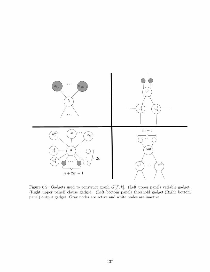
n+ 2m+ 1

2k...

u1

2

. . .

...

um2

. . .

✓

znzi

u1

1

vj

uj1 uj

2

zi

zi,1 zi,m+1

. . .

. . .

v1 vm

out

. . .

. . .

m� 1

Figure 6.2: Gadgets used to construct graph G[F , k]. (Left upper panel) variable gadget.(Right upper panel) clause gadget. (Left bottom panel) threshold gadget.(Right bottompanel) output gadget. Gray nodes are active and white nodes are inactive.

137

Lemma 6.22 Suppose that � 2 ⇢(F , k). Then, � satisfies that:

• For every i 2 {1, . . . , k}, �(i) is a variable node,• �(k + 1) is the threshold node,• For every i 2 {k + 2, . . . , 2m+ k + 1}, �(i) is a node in a clause gadget,• �(2m+ k + 2) is the output node.

Proof. First, observe that the output node of G[F , k] has degree 2m�1, with every neighborinitially inactive. Therefore, by the strict majority rule it is necessary to activate m of itsneighbors before activating it. As m� 1 of these neighbors are auxiliary output nodes, it isnecessary to activate the m clause nodes before activating the output node. Each clause nodehas degree 5, where one of the neighbors is the output node, and two neighbors are auxiliaryclause nodes, which are initially active. Therefore, the clause node requires that at least oneof the corresponding clause variable nodes is activated before it. Remember that the clausevariable nodes have degree three, where one neighbor is a clause node, another neighbor isthe threshold node, and the remaining one is a variable node. Consider now the time-stepon which for the first time a clause-variable node is updated. Then, this node requires thatboth the threshold node and the adjacent variable node are activated before it. Therefore,threshold must be changed to active during sequence �, and must become active before allthe clause variable nodes. The threshold node has degree 2n+4m+2k+1, with n+2m+1

adjacent auxiliary threshold nodes initially active and the remaining n+ 2m+ 2k neighborsinitially inactive. As we explained, 2m of its inactive neighbors are still inactive when thethreshold node is activated. Moreover, the 2k inactive auxiliary threshold nodes are alsoinactive when the threshold node is activated. Observe that the threshold node requires atleast k more active neighbors to become active. More precisely let p the amount of activeneighbors that are required to active threshold node. Then, we have that p must be chosenas the minimum number such the amount of active is more than the number of inactiveneighbors. Summarizing previous calculations we have (n+2m+1+ p) active neighbors and(n+ 2m+ 2k � p) inactive neighbors. Then, by asking p to satisfy (n+ 2m+ 1 + p)� (n+

2m+ 2k� p) > 0 we deduce p > k� 1

2and thus, p � k. We conclude that the only option is

to choose at least k variable nodes.

Wrapping up, we deduce the following order in every sequence activating the output nodein k + 2m + 2 steps: first, k variable nodes are activated. Then, the threshold node isactivated. Then, all the m clause nodes must be activated, which requires 2m steps, one forthe clause variable node, and one for the clause node. Finally the output node is activated.We deduce that � satisfies the statements of the lemma.

Lemma 6.23 Every � 2 ⇢(F , k) induces a truth-assignment in y 2 '(k,F). For everyy 2 '(k,F) there is a � 2 ⇢(F , k) that induces y.

Proof. Let � be a good sequence in ⇢(F , k). Lemma 6.22 implies that in a good sequenceevery clause node is activated, implying that at least one variable of each clause is chosenin the k first-steps. We deduce that � induces a truth-assignment of weight k satisfying F .Conversely, let y be a truth assignment in '(k,F). As this truth-assignment has weight k, we

138

Output gadget

Clause gadgets

Variable gadgets

Threshold gadget

Figure 6.3: Scheme representing graph G[F , k]. Each type of gadget is detailed in Figure 6.2.

can update the corresponding k variable nodes, and update the clause gadgets accordingly.This produces a sequence in ⇢(F , k).

Observe that Lemma 6.22 implies that for each truth-assignment y 2 '(F , k), there areseveral good sequences for v[F , k] with timespan t[F , k]. Indeed, we know that in the firstk time-steps the variable nodes that are true in y are updated. They can be updated inany order, so there are k! ways of updating them. Then, the threshold node is updated.Then, 2m nodes are updated to activate all clause nodes. Let us call � the number of waysthat the m clause nodes can be activated, once the k variable nodes and the threshold nodewere activated according to y. Unfortunately, the value of � is not easy to compute, since itdepends each the truth-assignment y. We say that a truth-assignment y fully satisfies clauseC if yc1 = yc2 = true, in other words, when both variables in the clause are true in y. Indeed,the exact value � depends on the number of clauses that are fully satisfied by a given truthassignment. A clause that is fully satisfied has two ways to be updated (one for each clausevariable node), while a clause that is not fully satisfied has only one.

Therefore, to be able to compute |'(F , k)| we will require to count with more detail.Let C = (c1 _ c2) be a clause of F . For d 2 [m] we call '(F , k, d) the set of truth-assignments of weight k satisfying F , and such that exactly d clauses of F are fully satisfied.Clearly |'(F , k)| =

Pmd=0

|'(F , k, d)|. Similarly, we define ⇢(F , k, d) as the number of goodsequences of v[F , k] with timespan t[F , k] that induce truth-assignments in '(F , k, d). Ob-viously |⇢(F , k)| =

Pmd=0

|⇢(F , k, d)|.

Lemma 6.24 |⇢(F , k, d)| = |'(F , k, d)| · k! · (2m)!

2m· 2d

Proof. Let us fix y 2 '(F , k, d). From Lemma 6.23 we know that y induces a good sequencein ⇢(F , k), and then by definition this sequence also belongs to ⇢(F , k, d). From Lemma 6.22we know that in the first k steps the variable nodes are updated. As they are independent,there are k! ways of updating the variables that are true in y. Once the k variable nodes areactivated, we have to continue by activating the threshold node. After that, we know fromLemma 6.22 that in the next 2m steps all the clause nodes must be activated.

139

For each clause, exactly two nodes are updated in the corresponding clause gadget. Indeedwe need 2 time steps to activate each clause node, and if we spend more than two steps inany clause gadget we are not going to be able to activate the output node in the timespan.Let C be the first clause. There are

�2m2

�ways of choosing steps to update one of its clause

variable nodes, and the clause node. To update the second clause, we have�2m�2

2

�ways of

choosing steps to update the corresponding pair. Repeating this argument we deduce thatthere are

mY

i=0

✓2m� 2i

2

◆=

2m!

2m

ways of choosing steps for updating a pair of nodes of each clause. Finally, for each fully-satisfied clause there are two possible choices of a clause-variable node to update, giving atotal of 2d choices.

Previous calculations imply that there are k! · (2m)!

2m· 2d possible good sequences that

induce y. We deduce that there are |'(F , k, d)| · k! · (2m)!

2m· 2d good-sequences inducing

truth-assignments in '(F , k, d).

Now let us call P (s) the degree m polynomial defined by

P (s) =mX

d=0

|'(F , k, d)|sd,

and observe that |⇢(F , k)| =Pm

d=0|⇢(F , k, d)| = (2m)!

2m· k! · P (2). We would like to compute

the coefficients of P (x). This is possible when we know an evaluation of the polynomial in alarge enough point, as notices by Valiant in [76]. For sake of completeness we give the resultand the full proof.

Lemma 6.25 Let P (x) =Pn

i=0aixi be a polynomial with integer coefficients upper bounded

by a A > 2. Suppose that we know a pair (x0, y0) such that y0 = P (x0) and x0 > A2.Then, there exists an algorithm that outputs the coefficients a0, . . . , an of P in a time that ispolynomial in n(log(x0) + log(y0) + log n).

Proof. First, observe thatPj�1

i=0aixi

0< xj

0. for every j 2 [n]. Indeed,

j�1X

i=0

aixi < A

j�1X

i=0

xi= Axj�1

j�1X

i=0

xi�j+1= Axj�1

j�1X

i=0

1

xj�1�i

< Axj�1

j�1X

i=0

1

A2i<

3

2Axj�1 < xj

0

Then, since an =y0�

Pn�1i=0 aixi

0

xn

0we deduce that,

y0xn0

� 1 < an y0xn0

implying that an =

�y0xn0

⌫.

140

We sequentailly obtain the other coefficients taking (x0, y0 � anxn0) as a pair for P 0

(x) =Pn�1

i=0aixi. From from Proposition 1.22 we deduce that each iteration can be done in time

log(x0) + log(y0) + log n.

Note that, unfortunately, the expression |⇢(F , k)| = (2m)!

2m· k! · P (2) only allows us to get

the value of the latter polynomial in s = 2 which is not a large-enough value to apply theprevious lemma. However, we can use a technique that is also inspired in the same paperof Valiant [76], used to show the #P-Completeness of a variant of SAT. Let p be a positiveinteger to be fixed later. Let Fp be the 2-CNF formula with n variables and mp clausesdefined as Fp

= F ^ F ^ · · · ^ F (repeated p times).

Lemma 6.26 |⇢(Fp, k)| = k! · (2mp)!

2mp· P (2

p)

Proof. Observe that F and Fp have the same set of variables, and each clause of F is repeatedp times on Fp. Therefore, '(Fp, k, pd) = '(F , k, d). Moreover, if d is not a multiple of p,then '(Fp, k, d) = ;. Then,

|⇢(Fp, k)| =mpX

d=0

|⇢(F p, k, d)|

=

mpX

d=0

|'(Fp, k, d)| · k! · (2mp)!

2mp· 2d

=

mX

d=0

|'(Fp, k, pd)| · k! · (2mp)!

2mp· 2pd

=

mX

d=0

|'(F , k, d)| · k! · (2mp)!

2mp· 2pd

= k! · (2mp)!

2mp· P (2

p)

Theorem 6.27 Contagion-Probability is #P-complete.

Proof. Let F be an instance of #Mon-2-Sat and consider the following algorithm comput-ing '(F) in polynomial time on a machine with an oracle for Contagion-Probability.For each k 2 [n], the algorithm picks p = 2n + 1 and constructs the input(G[Fp, k], x[Fp, k], v[Fp, k], t[F p, k]) of Contagion-Probability and queries the oracle on

it, obtaining |⇢(Fp, k)|. Then, the algorithm computes k! · (2mp)!

2mpand divides |⇢(Fp, k)| by

it in order to obtain the value P (2p) according to Lemma 6.26. Then, the algorithm uses as

141

a subroutine the algorithm given by Lemma 6.25 to obtain all the coefficients of P , whichcorrespond to {|'(F , k, d)|}d2{0,...,m}. Finally, the algorithm outputs

'(F) =

nX

k=1

mX

d=0

|'(F , k, d)|

From Proposition 1.22 and Lemma 6.25, all previous calculations can be done in poly-nomial time. We deduce that #Mon-2-Sat 2 FPContagion-Probability, implying thatContagion-Probability is #P-Complete.

6.2.2 Polynomial time algorithm for maximum degree 4

In this section, we restrict ourselves to the of Bootstrap Percolation in graphs of maximumdegree four. We show that in this case, unlike the general case studied in previous section, wecan compute the exact probability of infecting some node in polynomial time. Roughly, thismeans, that we are able to efficiently count the sequences of nodes, such that, if we updatethem we change the state of objective node from 0 to 1 in some fixed time t. In other words,we show that problem Contagion-Probability is in FP. To show this result, we use acharacterization given in [38], for the configurations where the objective node is unstable.This characterization involves a topological structure that can be exploited to design anefficient algorithm counting all the good sequences.

In the following, G = ([n], E) is a graph of degree at most 4, x is a configuration of {0, 1}nand v is a node such that xv = 0. We call G[0] the subgraph of G induced by the nodesthat are healthy, i.e. G[0] = G[{u 2 V : xu = 0}]. Observe that v 2 V (G[0]) and hencewe call G[0, v] the connected component of G[0] containing v. The following propositioncharacterizes the stable configurations.

Proposition 6.28 ([41]) Node v is stable in G if and only if v belongs to a path P in G[0]

such that an endpoint w of P belongs to a cycle in G[0] or dG(w) 2.

Suppose that v is a site that is not stable in G. For each neighbor w of v in G such thatxw = 0, we call Dw the connected component of G[v, 0]� v containing w. When xw = 1, wefix Dw = ;. The following lemma, characterizes the structure of the configuration aroundunstable sites.

Proposition 6.29 ([38]) Let w be a neighbor of v such that xw = 0 and w becomes activebefore v for some good sequence. Then Dw induces a tree of G[0] where all nodes have degreeat least 3 in G.

A component Dw which is a tree where all the nodes are of degree at least 3 in G is calleda good tree. As convention, an empty set is a good tree. Let GoodNeighbors(v) the set ofneighbors of v that induce good trees. Observe that v admits a good sequence if the strict

142

majority of its neighbors induce good trees. A tree of G[0] rooted at v is called a good treefor v, and denoted Tv, if Tv � v has

jdG(v)

2

k+ 1 components, each of them being good trees.

Definition 6.30 Given a tree T of size n rooted at r, a pruning sequence of T is a bijectivemapping ⇢ : [n] ! V (T ) such that, if u is an ancestor of v, then ⇢�1

(u) > ⇢�1(v). In

particular ⇢�1(r) = n. The number of pruning sequences of T is denoted #Prune(T, r).

The following lemma links up the good sequences of v with the existence of pruningsubsequences of the good trees in the neighborhood of v.

Lemma 6.31 A sequence � is a good sequence for v if and only there is a succession s1 <· · · < s|Tv | such that ⇢(i) := �(si) is a pruning sequence a good tree Tv of v.

Proof. Suppose first that � : [t] ! V is a good sequence for v and let {x(s)}s2[t] be thesuccession of configurations such that x(s) = F (x, �, s). Since � is a good sequence, theremust exist a step s⇤ 2 [t] in which v becomes infected, i.e. such that x(s⇤ � 1)v = 0 andx(s⇤)v = 1. In step s⇤ � 1 the strict majority of the neighbors of v must be infected.

From Proposition 6.29, we know that there exist a set {w1, . . . , wk} of k =

jdG(v)

2

k+ 1

neighbors of v such that, for all i 2 [k], node wi induces a good tree Di and x(s⇤ � 1)wi = 1.Define Tv = {v} [

Si2[k] Di, and observe that Tv is a good tree for v. Let us call s1 < · · · <

s` = s⇤ the sequence on which the nodes of Tv are updated, with ` = |Tv|. More precisely,for each j 2 [`] we have that �(sj) 2 Di, x(sj)�(sj) = 1 and x(sj � 1)�(sj) = 0. Observe that�(sj) is a leaf of Tv \ �([sj � 1]), because for each s 2 {s1 < · · · < s` = s⇤} state of node �(s)is updated, meaning that the majority of its children are infected or in state 1 in time s� 1

and also �(s) must be an ancestor of �(s) as any node in Tv was initially set to 0. Thus, ifsj is not a leaf of Tv \ �([sj � 1]) then, it would have more than one ancestor in Tv which isnot possible. We deduce that ⇢(i) := �(si) is a pruning sequence of Tv.

Conversely, if ⇢ is a pruning sequence of Tv, then in step s|Tv | vertex v becomes infected,implying that � is a good. sequence.

Now we introduce the main lemma of the section in which we computeContagion-Probability for an unstable node in a graphs of maximum degree 4. Ob-serve that, as we are considering the strict majority rule, a node that changes its state from 0

to 1 needs at least�dG(v)

2

⌫+1 neighbors in state one. Thus, we need to study two different

cases: the case in which a node changes from 0 to 1 with exactly�dG(v)

2

⌫+ 1 neighbors in

state one and the case in which there are more than that.

Lemma 6.32 Let (G, x, v, t) be an instance of Contagion-Probability such that G is agraph of maximum degree 4 and v is unstable. Then,

143

• If |GoodNeighbors(v)| =�dG(v)

2

⌫+ 1, then

Contagion-Probability(G, x, v, t) = ↵(T ⇤, v, t)

• If |GoodNeighbors(v)| >�dG(v)

2

⌫+ 1, then

Contagion-Probability(G, x, v, t) = ↵(T ⇤, v, t) + �(T ⇤, v, t)

where

↵(T, r, t) =

( �t|T |�#Prune(T, r) (n�|T |)!

(n�|T |�t)! if |T | t

0 otherwise,

�(T, r, t) =X

S⇢N(v)s.t|S|=dG(v)�1

(↵(TS, v, t)� ↵(T ⇤, v, t)),

T ⇤= {v} [

[

w2GoodNeighbors(v)

Dw and TS = {v} [[

w2S

Dw

Proof. First, for a given a rooted tree T , observe that ↵(T, r, t) is exactly the number ofsequences of length t that contain a pruning sequence of T . Indeed, if |T | > t then thisnumber is zero. Otherwise, a sequences containing a pruning of T is constructed picking |T |steps over the t possible choices, and prune T in the chosen steps. In the remaining stepsany other node can be updated. The number of ways that |T | steps can be picked over atotal of t steps is

�t|T |�. The possible ways of pruning the T on those steps is #Prune(T, v).

Finally, the number of possible choices for updating other vertices in the remaining steps is(n� |T |)!

(n� |T |� t)!. We deduce that ↵(T, r, v) is the product of previous quantities.

Lemma 6.31 implies that every good sequence for v contain a subsequence that canbe mapped into a pruning sequence of a good tree for v. When |GoodNeighbors(v)| =�dG(v)

2

⌫+ 1, there is only one possible choice of good tree for v, which is precisely

T ⇤= {v} [

Sw2GoodNeighbors(v) Dw. We deduce that the number of good sequences for v is

↵(T ⇤, v, t).

When |GoodNeighbors(v)| >

�dG(v)

2

⌫+ 1, then necessarily the degree of v is 3 or 4.

In either case |Good(v)| = d(v) and any good tree for v contains d(v) � 1 of its neighbors.Therefore, the choices for good sequences of v is the number of sequences that update containa prune of T ⇤, plus all the sequences that update some good tree of v, but not all T ⇤. Thenumber of sequences that contain a prune of T ⇤ is ↵(T ⇤, v, t). For a given set S of threeneighbors of v, the number of sequences that contain a pruning of the good trees inducedby the nodes in S, but not a pruning of T ⇤ equals ↵(TS, v, t) � ↵(T ⇤, v, t). We deduce thatContagion-Probability(G, x, v, t) equals

↵(T ⇤, v, t) +X

S⇢N(v)s.t|S|=3

(↵(TS, v, t)� ↵(T ⇤, v, t)).

144

Previous lemma implies that, in order to obtain a polynomial-time algorithm solving prob-lem Contagion-Probability, it is enough to have a polynomial-time algorithm computingthe value of #Prune(T, r, t), for a given rooted tree T . The following lemma states that thisis the case.

Lemma 6.33 Given tree T rooted in vertex r with maximum degree 4, there is an algorithmcomputing #Prune(T, r) in deterministic time polynomial in |T |.

Proof. For a node u in T , let us define the depth of u, denoted D(u), is the distance of u tothe root r. We also call M the maximum depth of a node in T . The function D(·) can becomputed in polynomial time simply running a BFS starting at node r. The level of a nodeu, denoted L(u), equals M �D(u). In other words, vertices at depth M are at level 0. Theroot is at level M .

Observe that all the nodes in level 0 are leafs, but not necessarily all leaves are at that level.For a given u 2 T , we call Tu the subtree rooted at u containing u and all it descendants.Observe that if u is a leaf of T , then #Prune(Tu, u) = 1. If u is not a leaf, let us callw1, . . . , wk the descendants of u in T , with k = d(u)� 1. Then,

#Prune(Tu, u) =(|Tw1 |+ · · ·+ |Twk

|)!|Tw1 |! · · · |Twk

|! #Prune(Tw1 , w1) · · ·#Prune(Twk, wk) (6.1)

Indeed, to #Prune(Tu, u) we have to prune all the descendants of u before u. Observethat a pruning of any two decendants of u are independent. Therefore, a pruning of Tu

consist in choosing |Tw| steps and a prune of Tw for each descendant w of u. For eachj 2 [k] let sj = |Twj

| and S = s1 + · · · + sk. Then, we have�Ss1

��S�s1s2

�· · ·

�S�

Pk�1j=1 sjsk

�=

�Ssk

� nQk=2

�S�

Pk�1j=1 sjsk

�=

(|Tw1 |+···+|Twk|)!

|Tw1 |!,...,|Twk|! ways of choosing |Tw| steps for every descendant w of u.

For each such choice, there are

#Prune(Tw1 , w1) · · ·#Prune(Twk, wk)

ways of choosing a pruning of each subtree Twi .

Therefore, our algorithm computing #Prune(T, r) consists in a dynamic programmingscheme over the levels of T . In level 0 all nodes u are leafs, and then #Prune(Tu, u) = 1. Ifall the nodes al level i are already computed, the value of #Prune(Tu, u) for a node in leveli + 1 can is computed using Equation 6.1.

Observe that for each u 2 T , the quantity #Prune(Tu, u) is at most |T |! = O(2|T | log |T |

).Therefore, from Proposition 1.22 we deduce that the expression of Equation 6.1 can becomputed in time O(|T |2). We conclude that #Prune(T, r) can be computed in timeO(|T |3).

145

Theorem 6.34 There is a polynomial-time algorithm solving Contagion-Probabilityrestricted to the graphs of maximum degree 4.

Proof. Let (G, x, v, t) be an input of Contagion-Probability, where G an n-node graphof maximum degree 4, x is a configuration of G, v is a node such that xv = 0 and t n.

The algorithm computes G[0, v], which is the component of G[0] that contains v. LetC1, . . . , Ck, with k 4 the connected components of G[0, v] � v. Then, it computesGoodNeighbors(v) verifying which components induce good trees. If |GoodNeighbors| <bd(v)

2c+ 1 then by Proposition 6.28 and Proposition 6.29, the algorithm outputs 0 because v

is stable. Now suppose |GoodNeighbors| � bd(v)2c + 1 then, for each w 2 GoodNeighbors(v),

compute #Prune(Tw, w), where Tw is the component (good tree) of G[0, v]�v that containsw. Finally, the output is computed according to the expressions given in Lemma 6.32. FromProposition 1.22 and Lemma 6.33, we deduce that our algorithm runs in time O(n3

).

146

Discussion

During this thesis work, we have developed a theoretical background to study the dynamicsof automata networks from a computational complexity viewpoint. In order to achieve thistask, we have studied in Chapter 2 how to precisely represent an automata network familyand how to manage different representations. In addition, we have proposed different variantsfor prediction problem and we have formalized the study of the computational and dynamicalproperties of abstract families of automata networks. In addition, we have shown that bothcomputational and dynamical properties are related thanks to the concept of simulation andparticularly thanks to the study of (strongly) universal networks.

Then, in Chapter 3 we have focused on how localized behavior in automata networkscan be analyzed in order to deduce global properties for a family of automata networks.We have identified the structure of a gadget and we have provided sufficient conditionsfor gadgets to form networks capable of coherently combine, from a dynamical viewpoint, itsparticular properties. Moreover, we have stated these conditions in the context of a frameworkwhich also opens new perspectives for future work. Additionally, we have presented concreteexamples of useful families such as Gm-networks and Gm,2-networks which allow us to definea concrete approach in order to study automata networks consisting, on the one hand, inanalyzing the period of attractors in order to find global bounds on this parameter and, onthe other hand, in searching for coherent Gm,2 (or Gm)-gadgets.

In Chapter 4, we have addressed the problem of asynchronism in the dynamics by devel-oping a framework based on the concept of projection systems and asynchronous extensions.We have presented a way to harmonize asynchronous dynamics by seeing it as a projectionof a synchronous dynamics defined over a large alphabet which contains the information onhow to updated different nodes at each time step.

Then, in Chapter 5, we have applied the theoretical framework developed on the latterchapters in order to systematically study a set of concrete symmetric automata network(CSAN) families under different update schemes. By constructing coherent gadgets andanalyzing dynamical properties, we have found some kind of marker for universality basedon an interesting trade-off between constraints in the update scheme and the simplicity ofrules. This observation combined with the description and properties of CSAN rules, suggestthat update schemes play an impactful role in changing the interaction graph by affecting itssymmetry and thus, symmetry plays an important role on the global properties of automatanetworks.

Finally, on chapter 6, we turned our attention to the structure of the interaction graph in

147

the context of the study of freezing dynamics.

In first place, we have established how alphabet size, treewidth and maximum degree ofthe underlying graph are key parameters which have an impact on the overall computationalcomplexity of finite freezing automata networks. We have accomplished this by definingthe Specification Checking Problem, that captures many classical decision problems such asprediction, nilpotency, predecessor, asynchronous reachability. We have presented a fast-parallel algorithm that solves this latter problem when the three parameters are bounded,hence showing that the problem is in NC. Moreover, we have shown that the problem is inXP on the parameters tree-width and maximum degree. Finally, we have hown that theseproblems are hard from two different perspectives. First, the general problem is W[2]-hardwhen taking either treewidth or alphabet as single parameter and fixing the others. Second,the classical problems are hard in their respective classes when restricted to families of graphwith sufficiently large treewidth. Moreover, for prediction, predecessor and asynchronousreachability, we establish the hardness result with a fixed set-defined update rule that isuniversally hard on any input graph of such families.

In the second part of this chapter we have studied the computational com-plexity of the problem Contagion-Probability. In general, we have shown thatContagion-Probability is #P-complete. Roughly speaking, this means there is no betterstrategy for computing the probability of an inactive node to change to state 1 than sim-ply simulate the system for each possible updating sequence � in order to verify how manyof them actually change the state of objective node. However, when we consider networkswith maximum degree 4, we have shown, based on previous results that characterize goodsequences in terms of underlying graph topology [38], that latter computation can be madein polynomial time.

Perspectives

Regarding our framework for glueing of automata networks it would be relevant to understandthe properties of a glueing process defined generally and see what kinds of properties can bededuced from it when considered as a process beyond the given conditions assuring coherenceof dynamics. Particularly, given two abstract automata networks belonging to some particularfamilies it would interesting to study at which point dynamical properties are preservedwhen two networks are glued. In addition, it would be very interesting to explore if latterprocess can be seen in the opposite way, i.e., given an automata network, determine if it ispossible to decompose the network in blocks satisfying some particular properties as gadgetsdo. Additionally, Proposition 3.19 provides an interesting starting point to explore the linkbetween different gate sets from the viewpoint of analyzing the richness of their synchronousclosure. This latter observation could lead to establish some sort of hierarchy between setsof gates. In this sense, it would be interesting to study, for example, reversible gate sets suchas Toffoli or Fredkin gates.

On the other hand, as we have pointed out in Chapter 4, it would be interesting to studyother types of update schemes which are not captured by general periodic update schemessuch as reaction-diffusion systems (see, for instance, [30]) or the most permissive semanticsintroduced in [15]. In both cases the orbits are not given by a choice in the possible nodes

148

that can be updated according to local rule. In that sense, it would be interesting to adaptthe concept of asynchronous extension in order to capture the latter update schemes.

Regarding our results on freezing automata networks, we observe that our algorithm forthe general model checking problem is not as efficient as known algorithms for specific sub-problems [11] and it would be interesting to establish hardness results in the NC hierarchy tomake this gap more precise. In the same vein, our algorithm does not yield fixed parametertractability results for any of the parameters (treewidth, degree, alphabet), and we wonderwhether our hardness results in the framework of parameterized complexity [23] could beimproved. We could also consider intermediate treewidth classes (non-constant but sub-polynomial). Concerning these complexity questions, we think that considering other (morerestrictive) parameters like pathwidth could definitely help to obtain better bounds.

Besides, one might wonder whether the set of dynamical properties that are efficientlydecidable on graphs of bounded degree and treewidth could be in fact much larger thanwhat gives our model checking formalism. This question remains largely open, but we canalready add ingredients in our formalism (for instance, a relational predicate representingthe input graph structure). However, we conjecture that there are NP-hard properties forfreezing automata network on trees of bounded degree that can be expressed in the followinglanguage: first order quantification on configurations together with a reachability predicate(configuration y can be reached from x in the system).

In addition, we think that we can push our algorithm further and partly release the con-straint on maximum degree (for instance allowing a bounded number of nodes of unboundeddegree). This can however not work in the general model checking setting as shown inRemark 6.4.

Concerning asynchronous bootstrap percolation, the first natural question that arises iswhether this threshold in the maximum degree of the network is tight, or in other words: isContagion-Probability still #P-complete even when restricted to instances of maximumdegree 5? Observe that gadgets in section 3 strongly use high connectivity in graph G[F , k] inorder to assure that good sequences will respect a fixed order while updating different nodesin the network (first we update variable nodes, then we update threshold gadget, etc.). Thisis a key aspect of the proof since it helps us to keep control in the amount different sequencesassociated to one particular assignation satisfying the Boolean formula. This shows thateven when one could conjecture a way to implement constant degree gadgets (by for exampleconsidering more copies of smaller gadgets) there should also be a way to keep track in allpossible good sequences that implement the same assignation satisfying the original Booleanformula.

Additionally, it could be also interesting to study a different version of problemContagion-Probability but now considering some other model having a different familyof automta networks such as CSAN networks, particularly, conjunctive or disjuntive net-works, algebraic networks or totalistic networks. In this regard, we recall that for some ofthe latter automata networks, there exist efficient algorithms (polynomial or even fast paral-lel algorithms) in order to compute the dynamics of the system (for example, in the case ofalgebraic networks or even conjunctive networks, it suffices to compute powers of some ma-trix). However, this does not necessarily implies that counting version of Good-Sequence

149

would be efficiently solvable.

In addition, we would like to note that the previous results are also interesting in thecontext of counting decision problems. Within this framework, we are no longer interested incomputing the number of all possible polynomial size certificates but to determine whether,for some fixed input, the majority of polynomial size strings we give to the verifier alongwith the input are actually certificates. This notion defines the complexity class PP. Moreprecisely a language L ✓ {0, 1}⇤ is in PP if and only if there exists a polynomial functionp : N! N and a polynomial-time verifier V such that x 2 L () |y 2 {0, 1}p(|x|) : V (x, y) =1| � 1

2·2p(|x|). By considering this formalism, a natural question arises: is the decision version

of Contagion-Probability which consists in deciding if the probability of transmissionfor objective node is at least 1

2, PP-complete? (observe that by definition it is in PP). In

this context, it is known that problem MAJ-SAT, which consist on deciding if the majorityof all assignments of some Boolean formula will satisfy it, is PP-complete and thus, it couldbe very interesting to explore as future work if an application of the same techniques we haveused in Section 3 might produce a polynomial-time reduction from latter problem to decisionversion of Contagion-Probability.

Finally, as we have shown that Contagion-Probability is #P-complete, it could beinteresting to study approximations. In particular, within the framework of applications onecould ask whether this problem admits a polynomial randomized approximation scheme.

150

Bibliography

[1] Hamed Amini and Nikolaos Fountoulakis. Bootstrap percolation in power-law randomgraphs. Journal of Statistical Physics, 155(1):72–92, feb 2014.

[2] Stefan Arnborg, Derek G. Corneil, and Andrzej Proskurowski. Complexity of findingembeddings in a k-tree. SIAM Journal on Algebraic Discrete Methods, 8(2):277–284,April 1987.

[3] Sanjeev Arora and Boaz Barak. Computational complexity: a modern approach. Cam-bridge University Press, 2009.

[4] Per Bak, Kan Chen, and Chao Tang. A forest-fire model and some thoughts on turbu-lence. Physics Letters A, 147(5):297 – 300, 1990.

[5] József Balogh and Béla Bollobás. Bootstrap percolation on the hypercube. ProbabilityTheory and Related Fields, 134(4):624–648, jul 2005.

[6] József Balogh, Béla Bollobás, Hugo Duminil-Copin, and Robert Morris. The sharpthreshold for bootstrap percolation in all dimensions. Transactions of the AmericanMathematical Society, 364(5):2667–2701, may 2012.

[7] József Balogh and Gábor Pete. Random disease on the square grid. Random Structures& Algorithms, 13(3-4):409–422, 1998.

[8] Edwin Roger Banks. Universality in cellular automata. In 11th Annual Symposium onSwitching and Automata Theory (swat 1970), pages 194–215. IEEE, 1970.

[9] Florent Becker, Diego Maldonado, Nicolas Ollinger, and Guillaume Theyssier. Univer-sality in freezing cellular automata. In Sailing Routes in the World of Computation - 14thConference on Computability in Europe, CiE 2018, Kiel, Germany, July 30 - August 3,2018, Proceedings, pages 50–59, 2018.

[10] Hans L. Bodlaender and Torben Hagerup. Parallel algorithms with optimal speedup forbounded treewidth. SIAM Journal on Computing, 27(6):1725–1746, December 1998.

[11] S. R. Buss. The boolean formula value problem is in ALOGTIME. In Proceedings of thenineteenth annual ACM conference on Theory of computing - STOC '87. ACM Press,1987.

151

[12] T. Calamoneri. The l(h,k)-labelling problem: A survey and annotated bibliography. TheComputer Journal, 49(5):585–608, February 2006.

[13] Olivier Carton, Bruno Guillon, and Fabian Reiter. Counter machines and distributedautomata. In Cellular Automata and Discrete Complex Systems, pages 13–28. SpringerInternational Publishing, 2018.

[14] John Chalupa, Paul L Leath, and Gary R Reich. Bootstrap percolation on a bethelattice. Journal of Physics C: Solid State Physics, 12(1):L31, 1979.

[15] Thomas Chatain, Stefan Haar, Loïc Paulevé, et al. Most permissive semantics of booleannetworks. arXiv preprint arXiv:1808.10240, 2018.

[16] Chandra Chekuri and Julia Chuzhoy. Polynomial bounds for the grid-minor theorem.Journal of the ACM, 63(5):1–65, dec 2016.

[17] Bruno Courcelle. The monadic second-order logic of graphs. i. recognizable sets of finitegraphs. Information and Computation, 85(1):12–75, mar 1990.

[18] Víctor Dalmau, Phokion G Kolaitis, and Moshe Y Vardi. Constraint satisfaction,bounded treewidth, and finite-variable logics. In International Conference on Principlesand Practice of Constraint Programming, pages 310–326. Springer, 2002.

[19] Bart De Schutter and Bart De Moor. On the sequence of consecutive powers of a matrixin a boolean algebra. SIAM Journal on Matrix Analysis and Applications, 21(1):328–354,1999.

[20] Jacques Demongeot and Sylvain Sené. About block-parallel boolean networks: a positionpaper. Natural Computing, 19(1):5–13, 2020.

[21] Alberto Dennunzio, Enrico Formenti, Luca Manzoni, Giancarlo Mauri, and Antonio E.Porreca. Computational complexity of finite asynchronous cellular automata. TheoreticalComputer Science, 664:131–143, February 2017.

[22] Rod G. Downey and Michael R. Fellows. Fixed-parameter tractability and completenessi: Basic results. SIAM Journal on Computing, 24(4):873–921, aug 1995.

[23] Rodney G. Downey and Michael R. Fellows. Fundamentals of Parameterized Complexity.Springer London, 2013.

[24] Michael Elberfeld, Andreas Jakoby, and Till Tantau. Logspace versions of the theoremsof bodlaender and courcelle. In 2010 IEEE 51st Annual Symposium on Foundations ofComputer Science. IEEE, October 2010.

[25] M.A. Fuentes and M.N. Kuperman. Cellular automata and epidemiological models withspatial dependence. Physica A: Statistical Mechanics and its Applications, 267(3–4):471– 486, 1999.

[26] Maximilien Gadouleau. On the influence of the interaction graph on a finite dynamical

152

system. Natural Computing, to appear.

[27] Maximilien Gadouleau and Adrien Richard. Simple dynamics on graphs. TheoreticalComputer Science, 628:62–77, may 2016.

[28] Andrew Goldberg, Serge Plotkin, and Gregory Shannon. Parallel symmetry-breaking insparse graphs. In Proceedings of the nineteenth annual ACM symposium on Theory ofcomputing, pages 315–324, 1987.

[29] Leslie M Goldschlager. The monotone and planar circuit value problems are log spacecomplete for p. ACM sigact news, 9(2):25–29, 1977.

[30] E Goles and Martin Matamala. Reaction-diffusion automata: Three states implies uni-versality. Theory of Computing Systems, 30(3):223–229, 1997.

[31] E. Goles, N. Ollinger, and G. Theyssier. Introducing freezing cellular automata. InExploratory Papers of Cellular Automata and Discrete Complex Systems (AUTOMATA2015), pages 65–73, 2015.

[32] Eric Goles, Fabiola Lobos, Gonzalo A Ruz, and Sylvain Sené. Attractor landscapes inboolean networks with firing memory: a theoretical study applied to genetic networks.Natural Computing, 19:295–319, 2020.

[33] Eric Goles, Diego Maldonado, Pedro Montealegre, and Nicolas Ollinger. On the com-putational complexity of the freezing non-strict majority automata. In Cellular Au-tomata and Discrete Complex Systems - 23rd IFIP WG 1.5 International Workshop,AUTOMATA 2017, Milan, Italy, June 7-9, 2017, Proceedings, pages 109–119, 2017.

[34] Eric Goles, Diego Maldonado, Pedro Montealegre, and Martín Ríos-Wilson. On thecomplexity of asynchronous freezing cellular automata. arXiv preprint arXiv:1910.10882,2019.

[35] Eric Goles, Diego Maldonado, Pedro Montealegre-Barba, and Nicolas Ollinger. Fast-parallel algorithms for freezing totalistic asynchronous cellular automata. In CellularAutomata - 13th International Conference on Cellular Automata for Research and In-dustry, ACRI 2018, Como, Italy, September 17-21, 2018, Proceedings, volume 11115 ofLecture Notes in Computer Science, pages 406–415. Springer, 2018.

[36] Eric Goles and Servet Martínez. Neural and Automata Networks: Dynamical Behaviorand Applications. Kluwer Academic Publishers, Norwell, MA, USA, 1990.

[37] Eric Goles and Pedro Montealegre. Computational complexity of threshold automatanetworks under different updating schemes. Theoretical Computer Science, 559:3–19,2014.

[38] Eric Goles and Pedro Montealegre. The complexity of the asynchronous prediction ofthe majority automata. Information and Computation, page 104537, 2020.

[39] Eric Goles, Pedro Montealegre, and Martín Ríos-Wilson. On the effects of firing memory

153

in the dynamics of conjunctive networks. Discrete & Continuous Dynamical Systems -A, 40(10):5765–5793, 2020.

[40] Eric Goles, Pedro Montealegre, Ville Salo, and Ilkka Törmä. Pspace-completeness ofmajority automata networks. Theoretical Computer Science, 609:118–128, 2016.

[41] Eric Goles, Pedro Montealegre-Barba, and Ioan Todinca. The complexity of the boot-straping percolation and other problems. Theoretical Computer Science, 504:73–82,2013.

[42] Eric Goles-Chacc, Françoise Fogelman-Soulié, and Didier Pellegrin. Decreasing energyfunctions as a tool for studying threshold networks. Discrete Applied Mathematics,12(3):261–277, 1985.

[43] Janko Gravner and David Griffeath. Cellular automaton growth on z2: Theorems,examples, and problems. Advances in Applied Mathematics, 21(2):241 – 304, 1998.

[44] Frederic Green. NP-complete problems in cellular automata. Complex Systems, 1, 011987.

[45] Raymond Greenlaw, H James Hoover, Walter L Ruzzo, et al. Limits to parallel compu-tation: P-completeness theory. Oxford University Press on Demand, 1995.

[46] D. Griffeath and C. Moore. Life without death is P-complete. Complex Systems, 10,1996.

[47] Godfrey Harold Hardy, Edward Maitland Wright, et al. An introduction to the theoryof numbers. Oxford university press, 1979.

[48] Alexander E. Holroyd. Sharp metastability threshold for two-dimensional bootstrappercolation. Probability Theory and Related Fields, 125(2):195–224, 2003.

[49] J Iirgen Albert and Karel Culik II. A simple universal cellular automaton and its one-wayand totalistic version. Complex Systems, 1:1–16, 1987.

[50] Joseph JáJá. An Introduction to Parallel Algorithms. Addison Wesley Longman Pub-lishing Co., Inc., USA, 1992.

[51] J. Kari. The Nilpotency Problem of One-dimensional Cellular Automata. SIAM Journalon Computing, 21:571–586, 1992.

[52] Akinori Kawachi, Mitsunori Ogihara, and Kei Uchizawa. Generalized predecessor ex-istence problems for boolean finite dynamical systems on directed graphs. TheoreticalComputer Science, 762:25–40, March 2019.

[53] William Ogilvy Kermack and A. G. McKendrick. A contribution to the mathematicaltheory of epidemics. Proceedings of the Royal Society of London. Series A, ContainingPapers of a Mathematical and Physical Character, 115(772):700–721, aug 1927.

154

[54] D. KNOP, M. KOUTECKÝ, T. MASAŘÍK, and T. TOUFAR. Simplified algorithmicmetatheorems beyond mso: Treewidth and neighborhood diversity. Logical Methods inComputer Science ; Volume 15, pages Issue 4 ; 1860–5974, 2019.

[55] Stephan Kreutzer and Siamak Tazari. On brambles, grid-like minors, and parameter-ized intractability of monadic second-order logic. In Proceedings of the Twenty-FirstAnnual ACM-SIAM Symposium on Discrete Algorithms, SODA 2010, Austin, Texas,USA, January 17-19, 2010, pages 354–364. SIAM, 2010.

[56] Martin Kutrib and Andreas Malcher. Cellular automata with sparse communication.Theor. Comput. Sci., 411(38-39):3516–3526, 2010.

[57] Kristian Lindgren and Mats G Nordahl. Universal computation in simple one-dimensional cellular automata. Complex Systems, 4(3):299–318, 1990.

[58] Noam Livne. A note on -completeness of NP-witnessing relations. Information Process-ing Letters, 109(5):259–261, February 2009.

[59] Dániel Marx. Can you beat treewidth? In 48th Annual IEEE Symposium on Foundationsof Computer Science (FOCS’07), pages 169–179. IEEE, 2007.

[60] Jacques Mazoyer and Ivan Rapaport. Inducing an order on cellular automata by agrouping operation. Discrete Applied Mathematics, 91(1-3):177–196, 1999.

[61] Cristopher Moore. Majority-vote cellular automata, ising dynamics, and p-completeness.Journal of Statistical Physics, 88(3/4):795–805, August 1997.

[62] Mathilde Noual. Updating automata networks. PhD thesis, École normale supérieure deLyon, 2012.

[63] Mathilde Noual and Sylvain Sené. Synchronism versus asynchronism in monotonicBoolean automata networks. Natural Computing, 17:393–402, 2018.

[64] Nicolas Ollinger. Toward an algorithmic classification of cellular automata dynamics.Reasearch report, 10, 2001.

[65] Nicolas Ollinger. The intrinsic universality problem of one-dimensional cellular au-tomata. In Annual Symposium on Theoretical Aspects of Computer Science, pages632–641. Springer, 2003.

[66] Nicolas Ollinger and Guillaume Theyssier. Freezing, bounded-change and convergentcellular automata. CoRR, abs/1908.06751, 2019.

[67] Loïc Paulevé and Sylvain Sené. Non-deterministic updates of Boolean networks. 2021.Submitted.

[68] Omer Reingold. Undirected connectivity in log-space. Journal of the ACM, 55(4):1–24,September 2008.

155

[69] Élisabeth Remy, Paul Ruet, and Denis Thieffry. Graphic requirements for multista-bility and attractive cycles in a boolean dynamical framework. Advances in AppliedMathematics, 41(3):335–350, 2008.

[70] Adrien Richard. Nilpotent dynamics on signed interaction graphs and weak conversesof thomas’ rules. Discrete Applied Mathematics, 267:160–175, aug 2019.

[71] Neil Robertson and P.D Seymour. Graph minors. v. excluding a planar graph. Journalof Combinatorial Theory, Series B, 41(1):92–114, aug 1986.

[72] Marko Samer and Stefan Szeider. Constraint satisfaction with bounded treewidth revis-ited. Journal of Computer and System Sciences, 76(2):103–114, 2010.

[73] Stefan Szeider. On fixed-parameter tractable parameterizations of SAT. In Theory andApplications of Satisfiability Testing, pages 188–202. Springer Berlin Heidelberg, 2004.

[74] Michael Treaster, William Conner, Indranil Gupta, and Klara Nahrstedt. Contagalert:using contagion theory for adaptive, distributed alert propagation. In Fifth IEEE Inter-national Symposium on Network Computing and Applications (NCA’06), pages 126–136.IEEE, 2006.

[75] S. M. Ulam. On some mathematical problems connected with patterns of growth offigures. In A. W. Bukrs, editor, Essays on Cellular Automata, pages 219–231. U. ofIllinois Press, 1970.

[76] Leslie G Valiant. The complexity of enumeration and reliability problems. SIAM Journalon Computing, 8(3):410–421, 1979.

[77] R. Vollmar. On cellular automata with a finite number of state changes. In ParallelProcesses and Related Automata / Parallele Prozesse und damit zusammenhängendeAutomaten, volume 3 of Computing Supplementum, pages 181–191. Springer Vienna,1981.

[78] Andrew Winslow. A brief tour of theoretical tile self-assembly. In Cellular Automata andDiscrete Complex Systems - 22nd IFIP WG 1.5 International Workshop, AUTOMATA2016, Zurich, Switzerland, June 15-17, 2016, Proceedings, pages 26–31, 2016.

[79] Angela Wu and Azriel Rosenfeld. Cellular graph automata. i. basic concepts, graphproperty measurement, closure properties. Information and Control, 42(3):305 – 329,1979.

[80] Angela Wu and Azriel Rosenfeld. Cellular graph automata. ii. graph and subgraphisomorphism, graph structure recognition. Information and Control, 42:330–353, 091979.

156