on information extraction principles for hyperspectral datalandgreb/whitepaper.pdf · on...

On Information Extraction Principles for Hyperspectral DataA White Paper

byDavid Landgrebe

School of Electrical & Computer EngineeringPurdue University

West Lafayette IN [email protected]

Preface

Means for optimally analyzing hyperspectral data has been the topic of a study of ourssince 19861. The point of departure for this study has been that of signal theory andthe signal processing principles that have grown primarily from the communicationsciences area over the last half century. The basic approach has been to seek a morefundamental understanding of high dimensional signal spaces in the context of theremote sensing problem, and then to use that knowledge to extend the methods ofconventional multispectral analysis to the hyperspectral domain in an optimal or nearoptimal fashion. The purpose of this white paper is to outline what has been learnedso far in this effort.

The introduction of hyperspectral sensors which produce much more complex datathan those previously should provide much enhanced abilities to extract usefulinformation from the data stream they produce. However, it is also the case that thismore complex data requires more complex and sophisticated data analysisprocedures if their full potential is to be achieved. Much of what has been learnedabout the necessary procedures is not particularly intuitive, and indeed, in many casesis counter-intuitive. In what follows, we shall attempt not only to illuminate some ofthese counter-intuitive aspects, but to make them clear and therefore acceptable.

1 Work leading to the material presented here was funded in part by NASA Grants NAGW-925(1986-94), NAG5-3975(1994-97), and ongoing Grant NAG5-3975.

©1997 by David Landgrebe - 1 - Printed July 25, 1997

Hyperspectral Data Analysis Principles

A System Overview

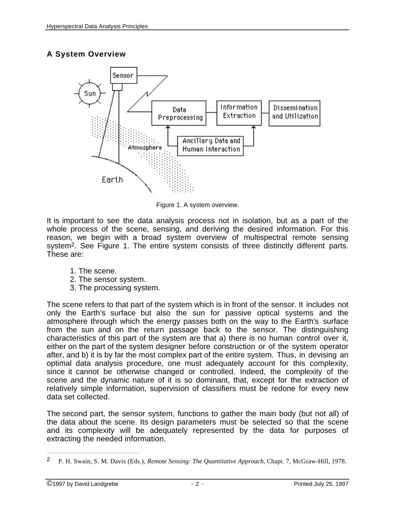
Figure 1. A system overview.

It is important to see the data analysis process not in isolation, but as a part of thewhole process of the scene, sensing, and deriving the desired information. For thisreason, we begin with a broad system overview of multispectral remote sensingsystem2. See Figure 1. The entire system consists of three distinctly different parts.These are:

1. The scene.2. The sensor system.3. The processing system.

The scene refers to that part of the system which is in front of the sensor. It includes notonly the Earth’s surface but also the sun for passive optical systems and theatmosphere through which the energy passes both on the way to the Earth's surfacefrom the sun and on the return passage back to the sensor. The distinguishingcharacteristics of this part of the system are that a) there is no human control over it,either on the part of the system designer before construction or of the system operatorafter, and b) it is by far the most complex part of the entire system. Thus, in devising anoptimal data analysis procedure, one must adequately account for this complexity,since it cannot be otherwise changed or controlled. Indeed, the complexity of thescene and the dynamic nature of it is so dominant, that, except for the extraction ofrelatively simple information, supervision of classifiers must be redone for every newdata set collected.

The second part, the sensor system, functions to gather the main body (but not all) ofthe data about the scene. Its design parameters must be selected so that the sceneand its complexity will be adequately represented by the data for purposes ofextracting the needed information.

2 P. H. Swain, S. M. Davis (Eds.), Remote Sensing: The Quantitative Approach, Chapt. 7, McGraw-Hill, 1978.



All of the remainder of the system, occurring after the sensor system in the data stream,we will refer to as the processing system.

Key System Parameters

In using an optimum systems approach, an important element is to have an adequatemodel of the system that is to be optimized3,4. Such quantitative models formultispectral remote sensing systems have been devised. While it would seeminappropriate to include them in this overview discussion, it is useful to provide a bitmore detail on the overall system than above, this time focused more on theinformation content of a data stream. For this purpose, we next list the key parametersof such an information system. They are,

1. The spatial sampling scheme. How is the scene to be sampled spatially?2. The spectral sampling scheme. How are the pixels to be sampled spectrally?3. The signal-to-noise ratio, S/N. What is the relation of the information-bearing

aspects of the sensed data to the non-information-bearing aspects.4. The ancillary information available. How will the classification process be

supervised?5. The informational classes desired and their interrelationships. What information

is desired as output and how complex is it.

An important characteristic of this list is that all five members of this list are interrelated.For example, the first three are obviously related through the principle of conservationof energy. The amount of energy emanating from the surface per unit area and per unitwavelength is finite. If one asks for very fine spatial resolution and at the same time avery narrow spectral band, then there is very little energy per pixel to overcome thenoise generated in the sensor detector. The interrelationship of the last two in this listwith the first three is perhaps a little less obvious. This relationship will be made clearshortly.

As a practical matter, how well an analysis process can work depends also on theanalyst, his/her expectations, initial assumptions, and point of view. We will commentonly briefly on these to demonstrate there impact on the analysis process.

Initial Assumptions About Multispectral Data Analysis

Some key questions to illuminate this issue are the following.

A. How does one visualize or view multispectral data?B. What does the data really look like in N-dimensional feature space?C. What is the explanation for the scatter of the data in N-dimensional space?

3 John Kerekes and David Landgrebe "Modeling, Simulation, and Analysis of Optical Remote Sensing Systems,"(PhD Thesis) Technical Report TR-EE 89-49, Purdue School of Electrical Engineering, August 1989.

4 John P. Kerekes and David A. Landgrebe, "Simulation of Optical Remote Sensing Systems," IEEETransactions on Geoscience and Remote Sensing, Vol. 27, No. 6, pp. 762-771, November 1989.



D. What relationship between the data complexity and the type of analysisalgorithm is most appropriate?

We will briefly examine each of these.

The matter of how the variations are represented mathematically and conceptually isan important first step in defining how the analysis process should proceed. Therehave been three principal ways in which multispectral data is representedquantitatively and visualized. See Figure 2 below.

• In image form, i. e., pixels displayed in geometric relationship to one another,• As spectra, i. e., variations within pixels as a function of wavelength,• In feature space, i. e., pixels displayed as points in an N-dimensional space.

We will refer to these three as image space, spectral space and feature space, andnext summarize some of the ramifications of these three perspectives.

Image Space Spectral Space Feature Space

Figure 2. The forms for representing multispectral data.

Image Space. Though the image form is perhaps the first form one thinks of when firstconsidering remote sensing as a source of information, its principal value has beensomewhat ancillary to the central question of deriving thematic information from thedata. Data in image form serve as the human/data interface in that image space helpsthe user to make the connection between individual pixel areas and the surface coverclass they represent. It also provides for supporting area mensuration activities usuallyassociated with use of remote sensing techniques. Thus, it becomes very important asto how accurately the true geometry of the scene is portrayed in the data. However, it isthe latter two of the three means for representing data that have been the point ofdeparture for most multispectral data analysis techniques.

Spectral Space. Many analysis algorithms which appear in the literature begin with arepresentation of a response function as a function of wavelength. Early in the work,the term "spectral matching" was often used, implying that the approach was tocompare an unknown spectrum with a series of pre-labeled spectra to determine amatch, and thereby to identify the unknown. This line of thinking has led, at various



times, to attempts to construct a "signature bank," a dictionary of candidate spectrawhose identity had been pre-established.

A second example of the use of spectral space is the "imaging spectrometer" concept,whereby identifiable features within a spectral response function, such as absorptionbands due to resonances at the molecular level, can be used to identify a materialassociated with a given spectrum. This approach, arising from the concepts ofchemical spectroscopy, which has long been used in the laboratory for molecularidentification, is perhaps one of the most fundamentally cause/effect basedapproaches to multispectral analysis.

Feature Space. The third basis for data representation also begins with a spectralfocus, i.e., that energy or reflectance vs. wavelength contains the desired information,but it is less related to pictures or graphs. It began by noting that the function of thesensor system inherently samples the continuous function of emitted and reflectedenergy vs. wavelength and converts it to a set of measurements associated with apixel which constitute a vector, i.e., a point in an N-dimensional vector space. Thisconversion of the information from a continuous function of wavelength to a discretepoint in a vector space is not only inherent in the operation of a multispectral sensor, itis very convenient if the data are to be analyzed by a machine-implemented algorithm.It, too, is quite fundamentally based, being one of the most basic concepts of signaltheory. Further, it is a convenient form if a more general form of feature extraction is toprecede the analysis step, itself. As will be seen below, of the three datarepresentations, the feature space provides the most powerful one from the standpointof information extraction.

Next, consider how multispectral data typically appears in feature space. We will use aparticularly simple situation to illustrate this. The graph below shows a scatter plot oftwo bands of Landsat Thematic Mapper data for an agricultural area. The areainvolved contains a small number of agricultural fields containing different species ofagricultural crops. One sees from this graph that, even though agricultural cropresponses are separable by appropriate means, this is not apparent from the scatterplot. The different crop responses do not manifest themselves as relatively distinctclusters. Rather, the data distributes itself more or less in a continuum over this space.This is typical of multispectral data, and indicates that the characteristics that allowdiscrimination between classes are more subtle than such straightforward examinationwould permit.



30

60

90

120

150

180

210

17 34 51 68 85 102

BiPlot of Channels 4 vs 3

Channel 3

+ + +++

+ ++++++ ++++

+ ++++

+++ +++

++++++

+++ +++ ++ + +++++ +++

+

+ +++++++

+++++ ++ +

+

+ +++ +

++

+

++

+++ +

++ + +++++ +++++ ++

+++++ +

++++ + + + + ++

++++++++

+ ++ ++ ++++

++++ +++++

+ + ++++ ++

+ +++

++++++

++

+ +

++

++++

+++++

++++

+++

++

++++++++

+ + + +++

++++++ +

++++++

+

+

+++++

+

+

+

++++

+++++

+

+

+

++

+++

+++

+++

++

+++++++

++++ +++ ++++++++ ++ ++

++++++

++ +++++ +++

+++

++ +++++++

+ ++

+++++++++++++

+

++++

++

++++++++

++++++++

++++ + +

+++

+

+++++++++

+++++++++++++++ +

++++

+

+

++ ++++++

++++

+++++

++ ++

+++++++ +

+ ++++++++++ + +

+

+++++++++

+ + +++

+++

++++++++++

++++ +++

+

++++++

++ +

++++

+++ +

+++++++

+ ++ ++

++ + +

+++ +

+

+++++++ +

+

+++

+

++ +++

+++

++++++++ +

++

+++

++++

++ +++++++++

+++++++ +++

++

++

++

+++++++ +

+

+

+

+ ++

++

++++++ + ++

+++

+++++++

++ +++++

++ + ++++++

+ +

+++++

++++

+++

++

++ +

++

++++

++++++

+

+++ +++

+

+

++++

+++++ +

++

+

+ +++

+++

+ +++

+

+

++ +

++++

+

++++

++++++

++++

+

++

++++++ +++++++ +++

+ +

+

+ +

++ +++

+++ +

++ ++

++ +++

++++

+++ ++

+++

+++

++

+

+++

+++++++ +

++

+++++ +

+

++

++++

+++

+ ++

+ +

++

+++

++

++++++ +

+++

+++

++

++++ +

+++

+++ + ++++

+++

++

++

++ +

+ + ++

+++++++

+

+++

+++++

+

+ + +

+++

+++ +

+

+ ++

+ ++

+

+++

+

+++

+++ +

++++++

+

++

+

+ ++

++

+

+

++

+

++++++ ++

+

+++

+

+

++

++

++ ++

++

++

+++

+

+++

+

+ +++++

+

++++

+++

+ ++

++

+++++++

++

+ ++

++

+++

++

++

+++ +

++

+ ++++

+ +++ +

+++

++++ +

++

+++

+

+ +

++++

+++

+ +

+++

+

+

++

+ +++ + +

+

++

+

++ ++

+++

+++

+

+

+++++

+

+++

++

++++ + +

++

+++++ +

+

+++++

++

+++

+++ ++++

+

+++

++

++

+ + ++

+ + ++

+

+

+++ ++

+

+ + +

+++

++ ++

+ + +

++ ++++++

++

+++++++

++++ ++

+++

++++

++++ +++

++

++ +

+

++ ++

+

+++

+++++++

++ + ++ +

+

++

++ +

+++

+

+++++++++++++

+

+++ ++

++++

++

+++

+++

++

+ ++

++++++

+++ +

+

+++

+ +

++

+++

+ ++

++

+ +++

+

+++

++++

++

+

++ +

+

+

++++

++++++

++

+

++ ++

++++++++++

++

++

+ +

+

++

++

+

++

++

++++

++ ++++

+

++

+ +

+

++++

+

++

++

+ + + ++

++

+ ++

+

++

+++

++

+++++

++

+

++++

+

+++

+++

+

+

+

++

+++

++++

+

+ ++

++

++ +

+

+

+++

++++

+

++

+

+

++

+++

+++

+

++

+

+ ++

++

+++

+++

++

+++

++

++

+ +++

++ +

++ ++

+ +

+++++++

+++

++

+ ++++++

+

+ +++

++++

++

++

++

+

++++++ +++

+

+ +

+ ++

+ ++

++

+++

++

++

+++

++

+++++++

+

++

+++

++

+ +

+

+

+

++++++

++

++

++

+

++

+

+

+

+

+++

+

+

+

++

+

++

++

+

+ +

+++

++

++++ +

+

+ +

+++

+

++

+

+

+

++

+

+

+++

+ +

+++

+

+

+

++++

+

++

++

++++

++ ++

++++

+

++ +

+ ++

+++

++

+ +

++++

+ ++ +

+

+++

++

++

+

++

+ +++

+

+ +

+ +++

+

++++

+++++++

+

+

+

++

+

++

+

+

++++

++

+

+

++ ++

+

++

++++++

+

+

+

++

+

+

+

+++++

++

+

++

++

+

++++

++

+

+

+

+

+

+

++

+

++

+++

++

++

+++++

++

+

+

+ ++

+ +

++

++

+++

+

+ +

+++

++++

++++++

++

++

+

+

+

+++

+

+++++ +

+

+

++ ++ ++

+

+ +++

+

+

+

+++

+ ++

++

+ +

+

+

++

+

+ +++ ++

+

+++++

+

+++

+

++

+

++

++

+

+

++ ++

++

+++++++

+

+

+

+

+

+++

+

+++

++++

++

++

++

+

++++ +

++ +

+

+

+

+

+

+

+++

+

+

+

+++++

+

+

+

++

+++

++

++++

+

++ +

+

++

++

++++ +

++

+++

+

++ +

+

+

+ ++ +

++

+

+

+

++

+

+

++

++

+

+

+++

++

+ +++

++

+

+

++

+

+++++ ++

+

+

+

+

++ ++++++++

++

+++

+

+

+++

+

+

++ ++

+

+

+

+++++

++

++

+

+++

++

+++ +

++

++

++

+

+

++

++++

+

+

+++ +++ +

+++

+

+

++

++

++

++++

+

+++++

+ ++++

++ +

+

+

+ ++

+

+++ +

++

++

++++ +

++

++ ++

++ ++++

++

++ ++

+++++

+

+++++ +

++

+

+ ++

+

+++

+

+++

+++

+ ++++

++

++ +++

+

++

+++

++

+++ +

+

++++

+++++++

+

+++

++ + +

++ ++

+ ++

+ +++++

++++

+++

+

+++

+

+

+++

++++ ++ +

+++

++ ++++++

+ ++

++

++

++

++ +

+ +++

+++

+

+

+++ ++++

+

++++++

+ ++ +

++++

++

+++

+ +++

+

++

+++

+++

++++

+++++++

+

+

++

++

++ ++++

+ +

+

+++

+

+++++

++++

+ ++

+

+

+

++ +++

++

+ +++++++ ++++

+ +++

+

++

+

++++

+

+

++

+++++

++ + +++

+

++

++

++ ++

+ +

+

++

+++ +

++

++

+

+++++

++ ++++

+ ++

+

+++ +

+

++

+++

+++ ++

++

+++++

++

+++++

+ + +

+++

+++++++ ++ + +

+ + +++++++++

+++

+++

+ ++

+

++++ +++++ ++

++++ +

++

++++

++ ++ ++++ +++

+++

+

++

+ +

+

+++

++

+

++++

++

+

++

++ +

++++

+++

++

++ +

++

++

++++

+

++++

+++

+

+

+

+

+

+

+ + ++ + + ++++

++

+ ++++ + ++ +

++

++

++++++ ++++

+

++++++++ ++

++++++

+

++

+

+

+

+

+

+

+

++ +++++

++

+ ++

+++++

++

++

++++++

+

+

+++

++

+++++++++++

+

+

++

++

+

++++++ +

++

++

+

++

++

+

+

+

+

+

+

++

+++++

+

++

+

++

++++

+

+

+

+

+

++++

++

+ +

+

++

++

+

+

+

+ ++

+

+++ +

+

+ +

++

++

++

+

+ ++

+

+

+

+

++

+

++

+

+

+

+

++

+++

+++

+

+++

+

+

+

+

++

++

++

+

++

++

+

++

+++ +

++

+

+++

+

++

+

+

+

++

+

++

+

++

+ +

+

+

+ + ++++

+

++

+ +

+

+

++ +

+

+

++

+

+

++

+

+

+ +

+

++++

+

+++

+

+

+

+++ +

++

+ +

+++

+

++

+

++

+ +++++

+

Figure 3. Scatter plot of TM Channel 4 (0.76-0.90 µm) vs. Channel 3 (0.63-0.69 µm)for an agricultural area containing a small number of crop types.

It also makes clear why entirely unsupervised classification schemes are not adequatefor multispectral discrimination purposes. Without guidance from the user as to whatclasses are desired to be identified, an unsupervised scheme will partition the spacein an unpredictable way. Further, we note that what appears to be random scatter isnot "noise," meaning harmful or even useless variability. This scatter is indeedinformation-bearing, if appropriate means are used to model it.

Another key characteristic which is fundamental to the engineering task of optimallydesigning a data analysis system is the basis for the mathematical representation ofthe data. A number of approaches have been considered for multispectral data overthe years. The following are some examples.

• Deterministic Approaches• Stochastic Models• Fuzzy Set Theory• Dempster-Shafer Theory of Evidence• Robust Methods, Theory of Capacities, Interval Valued Probabilities• Chaos Theory and Fractal Geometry• AI Techniques, Neural Networks

All of these approaches have been examined to varying degrees, and each hascertain facets which are attractive. Deterministic approaches, for example, tend to bethe most intuitive. This is important in a multidisciplinary field such as remote sensing,where different workers have different backgrounds. However, deterministic methodstend not to be as powerful, and may have other disadvantages such as being moresensitive to noise than is necessary.



Having investigated each, we have based our work on the stochastic or randomprocess approach5,6. This approach has the advantage of rigor and power, and, due toits maturity, has a large stable of tools that prove of pivotal usefulness in the work.

On the Significance of Second order Statistics

Use of a stochastic process approach for modeling the spectral response of a groundscene requires determining the necessary parameters for each given data set. Using aparametric model for such modeling thus reduces the problem to that of accuratelydetermining the mean vector and the covariance matrix in N-dimensional featurespace for each class of ground cover to be identified. Because of the centralimportance of this point, we shall illustrate this fact with several brief illustrativearguments.

1. First, as previously indicated, one of the advantages of the stochastic processapproach is the wealth of mathematical tools available using this method. Forexample, it is frequently the case that one would like to calculate the degree ofseparability of two spectral classes in order to project the accuracy it is possible toachieve in discriminating between them. There are available in the literature a numberof "statistical distance" measures for this purpose. They measure the statisticaldistance between two distributions of points in N-dimensional space. One withparticularly good characteristics for this purpose is the Bhattacharyya Distance. Inparametric form it is expressed as follows.

B = 18 [µ1-µ2]T[

Σ1+Σ22 ]-1[µ1-µ2] +

12 Ln

| 12[Σ1+Σ2] |

|Σ1| |Σ2|(1)

where µ i is the mean vector for class i and Σ i is the corresponding class covariancematrix. This distance measure bears a nearly linear, nearly one-to-one relationshipwith classification accuracy. Examining this equation, one sees that the first term onthe right indicates the part of the net class separability due to the difference in meanvalues of the two classes, while the second term indicates the portion of the totalseparability due to the class covariances. This makes clear from a quantitative point ofview what the relationship is between first order variations (the first term on the right)and second order variations (the second term on the right) is. This illustrates, forexample, that two classes can have the same mean value, in which case the first termis zero, and still be quite separable. Note that methods which are deterministicallybased only make use of separability measured by the first term.

2. A second way of seeing the importance of the second order variations in a moregraphical fashion is via the following example spectral data7. Shown in Figure 4 is aplot in spectral space of data from two classes of vegetation. These data weremeasured in the laboratory under well controlled circumstances so that the data

5 Cooper, G. R. & C. D. McGillem, Probabilistic Methods of Signal and System Analysis, Second Edition,Holt, Rinehart & Winston, 1986, Chapter 7.

6 Papoulis, A., Probability, Random Variables, and Stochastic Processes, Second Edition, McGraw-Hill 1984.7 P. H. Swain, S. M. Davis (Eds.), Remote Sensing: The Quantitative Approach, p. 14 ff, McGraw-Hill, 1978.



spread at each wavelength is not noise, but is due to the natural variability ofreflectance present from the leaves of such vegetation.

Figure 4. Spectral responses for a typical pair of classes, showing the interval at eachwavelength into which they fall.

It would appear from this spectral space view that the two classes are separable onlyin the region around 1.7 µm. However, even in the region around 0.7 µm where thereis maximum overlap of the two classes, they are separable classes if a method basedupon both the first and the second order effects is utilized.

To illuminate this further, in Figure 5 is shown the actual data values plotted in spectralspace for bands at 0.67 and 0.69 µm. It is clear from this presentation of the data thatthe reflectances do heavily overlap in these two bands.

0.720.710.700.690.680.670.660.6510

12

14

16

18

20

22

24

Class 1 - 0.67 µmClass 2 - 0.67 µmClass 1 - 0.69 µm

Class 2 - 0.69 µm

Scatter of 2-Class Data

Wavelength - µm

Ref

lect

ance

- %

|Figure 5. Data points for two vegetation classes in two spectral bands.

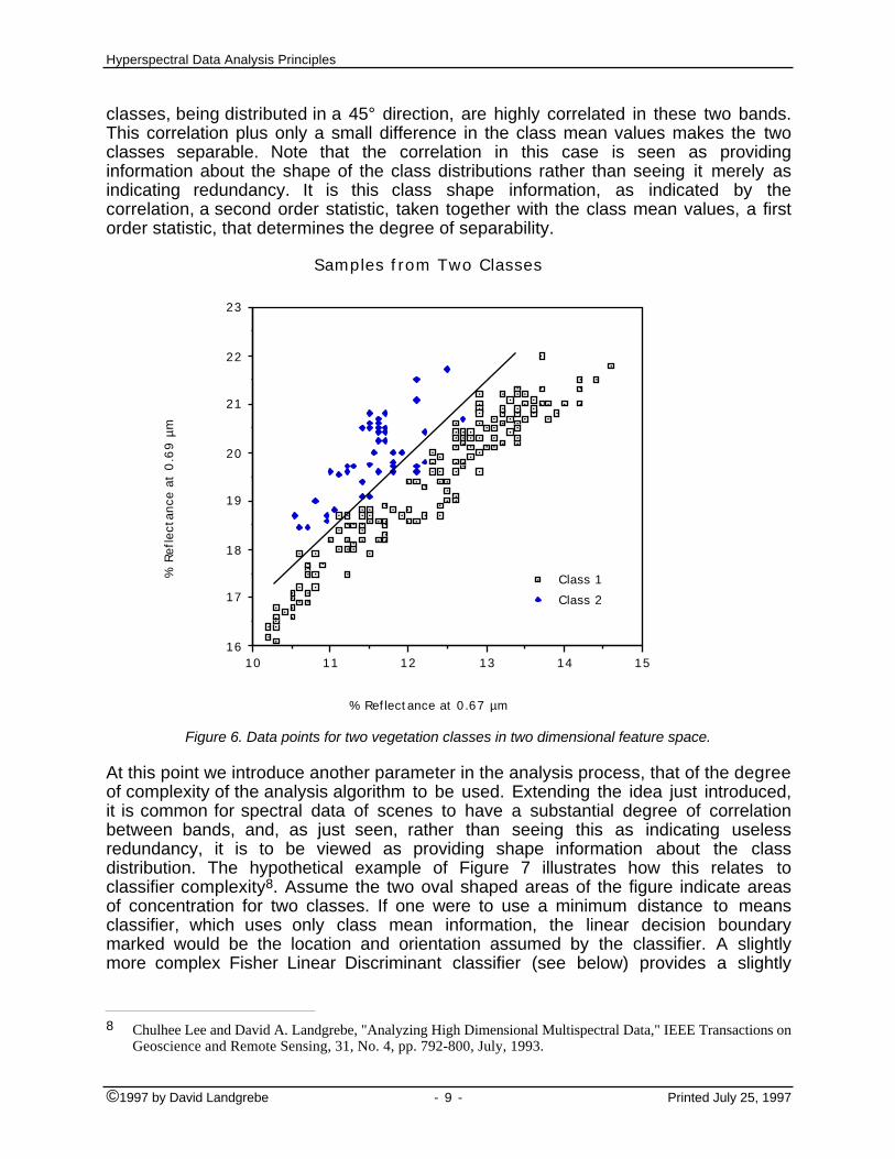
However, by plotting the same data in feature space as shown in Figure 6. it can beseen that the data are highly separable even via a simple linear classifier. Analyzingthis situation as to what allows this separability, one sees first that the data for both



classes, being distributed in a 45° direction, are highly correlated in these two bands.This correlation plus only a small difference in the class mean values makes the twoclasses separable. Note that the correlation in this case is seen as providinginformation about the shape of the class distributions rather than seeing it merely asindicating redundancy. It is this class shape information, as indicated by thecorrelation, a second order statistic, taken together with the class mean values, a firstorder statistic, that determines the degree of separability.

15141312111016

17

18

19

20

21

22

23

Class 1

Class 2

Samples from Two Classes

% Reflectance at 0.67 µm

% R

efle

ctan

ce a

t 0

.69

µm

Figure 6. Data points for two vegetation classes in two dimensional feature space.

At this point we introduce another parameter in the analysis process, that of the degreeof complexity of the analysis algorithm to be used. Extending the idea just introduced,it is common for spectral data of scenes to have a substantial degree of correlationbetween bands, and, as just seen, rather than seeing this as indicating uselessredundancy, it is to be viewed as providing shape information about the classdistribution. The hypothetical example of Figure 7 illustrates how this relates toclassifier complexity8. Assume the two oval shaped areas of the figure indicate areasof concentration for two classes. If one were to use a minimum distance to meansclassifier, which uses only class mean information, the linear decision boundarymarked would be the location and orientation assumed by the classifier. A slightlymore complex Fisher Linear Discriminant classifier (see below) provides a slightly

8 Chulhee Lee and David A. Landgrebe, "Analyzing High Dimensional Multispectral Data," IEEE Transactions onGeoscience and Remote Sensing, 31, No. 4, pp. 792-800, July, 1993.



shifted decision boundary as shown. The shaded areas would represent the pixelsthat would be classified incorrectly in this case.

If, on the other hand, one utilized a standard maximum likelihood Gaussian classifier,which utilizes both first and second order statistics, the curved decision boundarymarked would be the result with much improved error performance. We shall providegreater detail with regard to the matter of algorithm complexity shortly.

Decision boundary defined by the minimum distance classifier class

class

Decision boundary defined byGaussian ML classifier

Decision boundary defined byFisher's Linear Discriminant

ω

ω2

1

Figure 7. Example sources of classification error for the minimum distance classifierand maximum likelihood Gaussian classifiers.

3. The above example illustrates a concept in two dimensions, but what about higherdimensional data? This becomes more difficult to display intuitively, because onecannot draw in high dimensions. However, consider the following9.

9 David Landgrebe, "Multispectral Data Analysis: A Signal Theory Perspective," 43 pages, ©1994 by DavidLandgrebe, Downloadable from http://dynamo.ecn.purdue.edu/~biehl/MultiSpec/documentation.html



0

2

4

6

8

10

12

14

16

18

0.42 0.51 0.62 0.74 0.83 0.93 1.04 1.19 1.43 1.68 1.93

Re

lat

ive

Re

spo

ns

e

Wavelength - µm

Figure 8. A typical spectral reflectance curve for soil.

0

2

4

6

8

10

12

14

16

18

0.42 0.51 0.62 0.74 0.83 0.93 1.04 1.19 1.43 1.68 1.93

R

el

a

ti

ve

Re

s

po

ns

e

Wavelength - µm

Figure 9. Spectral responseshowing second order variations.

Shown in Figure 8 is a single spectral reflectance curve for a certain soil type inspectral space. Except for the two absorption bands, it appears rather featureless, andindeed, no second order effects can be seen from a single deterministic curve. Shownin Figure 9 is the result in spectral space of making five measurements on samples ofthis soil type. Some variation is now apparent, although its structure cannot bediscerned in this spectral space presentation. However, Figure 10 shows the result ofplotting the data of Figure 9 after have subtracted out the mean of the five samples,thus separating the first order statistic, the mean value, out so that structure in thesecond order variation can be more clearly observed. It is seen that the samples havea high degree of correlation in the region up to about 0.9 µm, in that a sample that isabove the mean at 0.5 µm tends to remain above the mean up to 0.9 µm, while onethat is below tends to remain below. Above 0.9 µm this structure changes significantly.If this structure should be diagnostic of this soil type in that no other material in thesame scene would have this same characteristic, then it would indicate a capability todiscriminate this soil type in that scene.

-1.5

- 1

-0.5

0

0.5

1

1.5

0.42 0.51 0.62 0.74 0.83 0.93 1.04 1.19 1.43 1.68 1.93

Figure 10. Second order variations about the mean for the samples of Figure 9

Though it is not possible to show a graph in the needed high dimensional featurespace, it is possible to determine quantitatively its separability from other classes, forexample, by using Bhattacharyya Distance, equation (1) above. Further, an additionalvisualization tool for high dimensional data has been devised and is referred to as"statistics image" 10




4. An example classification from a recent paper will further illuminate the matter11. Forthis experiment, a multispectral data set with a large number of spectral bands wasanalyzed using standard pattern recognition techniques. The data were classifiedusing first a single spectral feature, then two, and continuing on with greater andgreater numbers of features. Three different classification schemes were used, (a) astandard maximum likelihood Gaussian scheme, in which both the means and thecovariance matrices, i.e., both first and second order variations, were used, (b) thesame except with the mean values of all classes adjusted to be the same, so that theclasses differed only in their covariances, and (c) using a minimum distance to meansscheme such that mean differences are used, but covariances are ignored. It is seenfrom the results shown in Figure 11 below that case (a) produced clearly the bestresult, as would be expected.

20181614121086420

0

20

40

60

80

100

Number of Features

Cla

ssifi

catio

n A

ccur

acy

(%)

Gaussian ML (Mean & Cov) Gaussian ML (Cov Only) Minimum Distance Classifier

Figure. 11. Performance comparison of the Gaussian ML classifier, the GaussianML classifier with zero mean data, and the minimum distance classifier.

In comparing the latter two, though, it is seen that, at first in low dimensional space, theclassifier using mean differences performed best. However, as the number of featureswas increased, this performance soon saturated, and improved no further. On theother hand, while the classifier of case (b) which used only second order effects, wasat first the poorest, it soon outperformed the one of case (c) and its performancecontinued to improve as greater and greater numbers of features were used. Thus it isseen that second order effects, in this case represented by the class covariances, arenot particularly significant at low dimensionality, but they become so as the number offeatures grows, to the point that they become much more significant than the meandifferences between classes at any dimensionality. It is, of course, also possible to




show other example classifications where the mean vector dominates over thecovariance12.

These four examples show the added value of second order variations over first orderones alone, and the usefulness of an N-dimensional feature space view point. Eventhough one cannot draw in more than three dimensions, and thus "visualize" what istaking place, mathematical tools such as Bhattacharyya Distance are available toquantify what is the case in such spaces.

However, the potential advantage of second order effects can be easily lost ifincreased precision in determining the class distributions is not achieved. This is whatis dealt with in the following section.

Ancillary Information and Classifier Supervision.

From the vantage point of the above, it is clear that analysis methods which utilize bothfirst and second order statistics can provide superior performance compared to thosewhich utilize only first order effects. However, in many cases, this is not what isobserved in practice. The explanation for this becomes apparent from the followingadditional aspects of signal theory.

With regard to the ability to discriminate between a pair of classes, an illuminatingtheoretical result appeared in the literature some years ago13. In this paper, the resultshown in Figure 12 was derived. The ordinate for the curves in this figure is the meanrecognition accuracy for the two class case, averaged over the ensemble of classifiers.The abscissa is measurement complexity, which in the case of multispectral data, isdirectly related to the number of bands and the number of gray values per bands. Theparameter for the different curves of the graph is the prior probability of one of the twoclasses. Looking specifically at the case for the prior probability of one half, one seesthat the curve increases with measurement complexity, rapidly at first, but then moreslowly. However the curve does not have a maximum, implying that it continues toincrease.

12 Jimenez, Luis, and David Landgrebe, “Supervised Classification in High Dimensional Space: Geometrical,Statistical, and Asymptotical Properties of Multivariate Data,” IEEE Transactions on System, Man, andCybernetics, To appear January, 1998. Downloadable from

http://dynamo.ecn.purdue.edu/~biehl/MultiSpec/documentation.html13 G. F. Hughes, "On The Mean Accuracy Of Statistical Pattern Recognizers," IEEE Trans. Infor. Theory, Vol.

IT-14, No. 1, pp. 55-63, 1968



MEASUREMENT COMPLEXITY n (Total Discrete Values)

ME

AN

RE

CO

GN

ITIO

N A

CC

UR

AC

Y

1 2 5 10 20 50 100 2000

0.5

0.6

0.7

0.8

0.9

1.0

0.5

0.6

0.7

0.75

0.8

0.85

0.9

Pc =

Figure 12. Mean Recognition Accuracy vs. MeasurementComplexity for the infinite training case.

The graph of Figure 12 is for the case where there were an infinite number of trainingsamples available, implying completely precise knowledge of the class distributions.Dr. Hughes also derived the result for finite training data. The result is shown in Figure13 for the case of equally likely classes. Here the parameter for the various curves ism, the number of training samples. It is seen in this case that each curve (except for them → ∞ case) does have a maximum, indicating that there is a best measurementcomplexity. It depends upon how many training samples one has, and thus howprecise is the estimate of the class distributions.

It is important to note that the maximum of the curves moves upward and to the right asm increases, indicating that one can expect, on the average, to see improvedperformance as one increases the measurement complexity, but to achieve it, one willneed increased precision in estimating the class distributions.

m=2510

20

50100

200

1000

500

m = ∞

1 100050020010050201052

MEASUREMENT COMPLEXITY n (Total Discrete Values)

0.50

0.55

0.60

0.65

0.70

0.75

ME

AN

RE

CO

GN

ITIO

N A

CC

UR

AC

Y

Figure 13. Mean Recognition Accuracy vs. MeasurementComplexity for the finite training case.

This result, that shows that more spectral bands is not always better, and indeed, that itin fact becomes worse, was rather controversial when it was first introduced. The originof this phenomenon can be made more understandable by the following simpledrawings illustrating the basic concepts involved.



If one were to sketch the expected relationship between class separability anddimensionality, it should look something like Figure 14 (A), i.e. similar to Figure 12.Further, if one were to sketch the conceptual relationship between the accuracy ofstatistics estimation and dimensionality, it should be as in Figure 14 (B). That is, for afixed number of training samples, as one increases the dimensionality, one wouldexpect the accuracy of estimation to decline. For example, 100 samples may beenough to obtain a reasonably accurate estimate of the elements of a 5 dimensionalmean vector and covariance matrix, but it would not be enough for 500 dimensionalone. Further, if one increases the number of training samples, N1→N2, one wouldexpect the curve to shift to the right.

Dimensionality

Separ

abili

ty

Dimensionality

Acc

urac

y of

Sta

tist

ics

Esti

mat

ion

2N

1N

2N1N <

(A) (B)

Dimensionality

Cla

ssif

icat

ion

Acc

urac

y 2N

1N

(C)

Figure 14. Effects which result in the Hughes Phenomenon.

Taken together, these two factors would produce an overall relationship as shown inFigure 14 (C), a relationship not unlike that of Figure 13.

On Classifier Complexity

The Hughes result above again reflects not only on the need for precise classdistribution determination, but indirectly to a relationship between dimensionality andthe complexity of the classifier algorithm to be used. There is now a large array of



different types of classifier algorithms that appear in the literature. Often it is difficult todiscern from their description the extent to which they make use of the variousinformation-bearing attributes of the multispectral or hyperspectral data. Thus it seemsuseful to have a generic list of classifier algorithms given in an ascending hierarchicalorder according to the portion of the spectral attributes that they utilize. Then, as newor specialized algorithms are encountered, they can be compared with the hierarchy tobetter understand what portion of the possible signal attributes they utilize. In doing so,we shall assume that the data are in feature space vector form, and will not take intoaccount attributes other than spectral ones.

A standard way of describing a classification rule is to use the discriminant function.For the m-class case, where the pixel to be classified is specified as X, a vector infeature space, assume we have m functions of X, g1(X), g2(X), . . . gm(X) such thatgi(X) is larger than all others whenever X is from class i. These functions gi(X) arereferred to as discriminant functions. Then the classification rule becomes

Let ωi denote the i th class. Then decide X is in class ωi if and only ifgi(X) ≥ gj(X) for all j = 1,2, . . . m.

For those classifiers in the list which specifically involve the parameter estimators, weshall specify them in terms of the appropriate discriminate function.

1. Ad hoc and deterministic algorithms.

The nature of variations in spectral response which are usable for discriminationpurposes is quite varied. They may extend all the way from the general shape of theresponse function spread across many bands to very localized variations in one or asmall number of narrow spectral intervals. Many algorithms have appeared in theliterature which are designed to take advantage of specific characteristics on an adhoc basis. Example algorithms of this type extend from simple parallelepipedalgorithms or spectral matching schemes based upon least squares differencebetween an unknown pixel response that has been adjusted to reflectance and aknown spectral response from a field spectral data base, on to an imagingspectroscopy scheme based upon one or more known molecular absorption features.

Such algorithms are sometimes motivated by a desire to take advantage ofperceivable cause/effect relationships. These algorithms are usually of a nature thatthe class is defined by a single spectral curve, i.e., a single point in feature space.When this is the case, by that fact, they cannot utilize second order class information.

In the following parametric methods, X is the observed (vector-valued) pixel, µ i is themean vector for class i and Σ i is the corresponding class covariance matrix. It isassumed there are m classes, and, for simplicity for present purposes, the classes areassumed equally likely. In this case, given the additional assumptions specific to eachcase, these schemes are Bayes optimal in the sense that they will provide minimumerror for the class statistics given. They are suboptimal only to the extent that thevarious assumptions are not, in fact, met, and that the finite training sets do notcompletely precisely determine the class statistics.



2. Minimum Distance to Means

gi(X) = (X – µ i)T(X –µ i) (2)

choose class i if gi(X) ≤ gj(X) for all j = 1,2, . . . m.

In this case, pixels are assigned to whichever class has the smallest Euclideandistance to its mean. The classes are, by default, assumed to have commoncovariances which are equal to the identity matrix. This is equivalent to assuming theclasses all have unit variance in all features and the features are all uncorrlated to oneanother. The decision boundary in feature space will be linear and located equidistantbetween the class means and orthogonal to a line joining their means. See Figure 7.

3. Fisher's Linear Discriminant

gi(X) = (X – µ i)TΣ-1(X –µ i) (3)

choose class i if gi(X) ≤ gj(X) for all j = 1,2, . . . m.

In this case, the classes are assumed to have a common covariance specified by Σ.This is equivalent to assuming the classes do not have the same variance in allfeatures, the features are not necessarily uncorrlated, but both classes have the samevariance and correlation structure. In this case the decision boundary in feature spacewill be linear, but its location between the class mean values will depend upon Σ.

4. Quadratic (Gaussian) Classifiergi(X) = - (1/2)ln|Σ i| - (1/2)(X-µ i)TΣ i

-1(X-µ i) (4)

choose class i if gi(X) ≥ gj(X) for all j = 1,2, . . . m.

In this case, the classes are not assumed to have the same covariance, each beingspecified by Σ i. The decision boundary in feature space will be a second orderhypercurve (or several segments of second order hypercurves if more than onesubclass per class is assumed), and its form and location between the class meanvalues will depend upon the Σ i’s.

5. Nonparametric Methods

gi(X) = 1Ni

∑j=1

Ni

K(X–X ji

λ) (5)

choose class i if gi(X) ≥ gj(X) for all j = 1,2, . . . m.

Nonparametric classifiers take on many forms, and their key attractive feature is theirgenerality. As represented above, K(.) is a kernel function which can take on many



forms. The entire discriminate function has Ni terms, each of which may contain one ormore arbitrarily selected parameters. Thus, the characteristic which gives anonparametric scheme its generality is this often large number of features. However,every detailed aspect of the class density must be determined by this process, and thiscan quickly get out of hand. For example, while Fukunaga14 proves that in a givencircumstance, the required number of training samples is linearly related to thedimensionality for a linear classifier and to the square of the dimensionality for aquadratic classifier, in a nonparametric case, it has been estimated that as the numberof dimensions increases, the sample size needs to increase exponentially in order tohave an effective estimate of multivariate densities15,16. It is for this reason thatnonparametric schemes, including the currently popular neural network methods, areless attractive for the remote sensing circumstance, than they might at first appear. Inaddition, for neural network methods, which use iterative training, the large amount ofcomputation required in the training process detract from their practical value, sincetraining must be redone for every data set. As a result, we will focus on parametricmethods hereafter.

We again note that methods which use multiple samples for training have a substantialadvantage over deterministic methods that utilize only a single spectrum to define aclass. The latter tend to require very high signal-to-noise ratios, where as those basedupon multiple sample training sets tend to be more immune to the effects of noise.

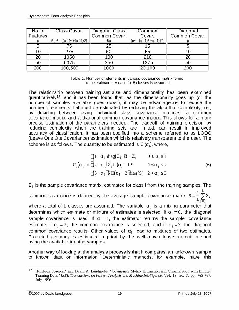
The means for quantitatively describing a class distribution from a finite number oftraining samples commonly comes down to estimating the elements of the class meanvector and covariance matrix, as has been seen. Sound practice dictates that thenumber of training samples must be large compared to the number of elements inthese matrices. When the number of training samples is limited, as it nearly always isin remote sensing, and the dimensionality of the data becomes large, the neededrelationship between the training set size and the number of matrix elements that mustbe estimated quickly becomes strained even in the parametric case. This is especiallytrue with regard to the covariance matrix, whose element population grows veryrapidly with dimensionality. For example, the following table illustrates the number ofelements in the various covariance matrix forms which must be estimated for the caseof 5 classes and several different numbers of features, p.

14 Fukunaga, K. "Introduction to Statistical Pattern Recognition." San Diego, California, Academic Press, Inc.,1990.

15 Scott, D. W. "Multivariate Density Estimation." John Wiley & Sons, pp. 208-212, 1992.16 Hwang, J., Lay, S., Lippman, A., "Nonparametric Multivariate Density Estimation: A Comparative Study.",

IEEE Transactions on Signal Processing, Vol. 42, No. 10, 1994, pp. 2795-2810.



No. ofFeatures

p

Class Covar.

5p2 – [(p-1)2 +(p-1)]/2

Diagonal ClassCommon Covar.

5p

CommonCovar.

p2 – [(p-1)2 +(p-1)]/2

DiagonalCommon Covar.

p

5 75 25 15 510 275 50 55 1020 1050 100 210 2050 6375 250 1275 50

200 100,500 1000 20,100 200

Table 1. Number of elements in various covariance matrix formsto be estimated. A case for 5 classes is assumed.

The relationship between training set size and dimensionality has been examinedquantitatively17, and it has been found that, as the dimensionality goes up (or thenumber of samples available goes down), it may be advantageous to reduce thenumber of elements that must be estimated by reducing the algorithm complexity, i.e.,by deciding between using individual class covariance matrices, a commoncovariance matrix, and a diagonal common covariance matrix. This allows for a moreprecise estimation of the parameters needed. The tradeoff of gaining precision byreducing complexity when the training sets are limited, can result in improvedaccuracy of classification. It has been codified into a scheme referred to as LOOC(Leave One Out Covariance) estimation which is relatively transparent to the user. Thescheme is as follows. The quantity to be estimated is Ci(αi), where,

C i α i( ) =

1 −α i( )diag Σ i( ) +α i Σi 0 ≤ αi ≤ 1

2 −α i( )Σ i + αi − 1( )S 1 <α i ≤ 2

3 −α i( )S + αi − 2( )diag(S) 2 <α i ≤ 3

(6)

Σ i is the sample covariance matrix, estimated for class i from the training samples. The

common covariance is defined by the average sample covariance matrix S =1

LΣ i

i =1

L

∑where a total of L classes are assumed. The variable αi is a mixing parameter thatdetermines which estimate or mixture of estimates is selected. If αi = 0, the diagonalsample covariance is used. If αi = 1, the estimator returns the sample covarianceestimate. If αi = 2, the common covariance is selected, and if αi = 3 the diagonalcommon covariance results. Other values of αi lead to mixtures of two estimates.Projected accuracy is estimated a priori by the well-known leave-one-out methodusing the available training samples.

Another way of looking at the analysis process is that it compares an unknown sampleto known data or information. Deterministic methods, for example, have this

17 Hoffbeck, Joseph P. and David A. Landgrebe, “Covariance Matrix Estimation and Classification with LimitedTraining Data,” IEEE Transactions on Pattern Analysis and Machine Intelligence, Vol. 18, no. 7, pp. 763-767,July 1996.



comparison taking place at the pixel to pixel or spectrum to spectrum level. The nextstep up in the effective utilization of reference data is a scheme which compares apixel to a class distribution. This is the function of procedures 2 through 5 above, andis the most common form of pixel classifiers. One can take the process one step furtherby using a scheme which results in distribution to distribution comparison. Thisscheme, sometimes called a sample classifier, requires that one have as the unknowna set of pixels which are all assumed to be members of the same class. Classifierswhich utilize spatial as well as spectral information can be arranged to operate in thisway. The ECHO classifier18,19 is an example of this case. It proceeds by firstsegmenting the scene on a multivariant basis into statistically homogeneous objectsusing spatial information, then classifying the objects using a distribution to distributioncomparison. Using the same class descriptions as a pixel classifier, it nearly alwaysachieves higher accuracy and usually does so with less computation time.

In addition to these methods, additional aspects of classifier design have beeninvestigated, including more complex decision logic20,21 and ways to speed theclassification computation22,23. With the rapid increase of computational processorspeeds in recent years, processing speed has turned out not to be the pressingproblem it once was, and until the more pressing problems of the analysis process aresolved, complex decision logic potentials can also reasonably be postponed. Thusthese aspects are being pursued at a lower priority.

One additional aspect of classifier design which appears to have significant utility hasalso been investigated. It has been shown24,25 that by adding unlabeled samples tothe classifier design process, better estimates for the discriminant functions can beobtained. This has resulted in an algorithm referred to as "statistics enhancement." Thealgorithm iterates between the labeled (training) samples and unlabeled (all other)samples from the data set to modify the class statistics so that a better fit to the overalldata distribution is obtained. In this way, the ability of the classifier to generalizebeyond its training samples is improved. In mathematical terms, what is desired is to

18 R. L. Kettig and D. A. Landgrebe, "Computer Classification of Remotely Sensed Multispectral Image Data byExtraction and Classification of Homogeneous Objects," IEEE Transactions on Geoscience Electronics, VolumeGE-14, No. 1, pp. 19-26, January 1976.

19 D. A. Landgrebe, "The Development of a Spectral-Spatial Classifier for Earth Observational Data," PatternRecognition, Vol. 12, No. 3, pp. 165-175,1980.

20 B. Kim and D. Landgrebe, "Hierarchical Classifier Design in High Dimensional Numerous Class Cases," IEEETransactions on Geoscience and Remote Sensing, Vol. 29, No. 4, July 1991, pp. 518-528.

21 S. Rasoul Safavian and David Landgrebe, "A Survey of Decision Tree Classifier Methodology," IEEETransactions on Systems, Man, and Cybernetics, Vol. 21, No. 3, May/June 1991, pp. 660-674.

22 Chulhee Lee and David A. Landgrebe, "Fast Likelihood Classification," IEEE Transactions on Geoscience andRemote Sensing, Vol. 29, No. 4, July 1991, pp. 509-517.

23 Byeungwoo Jeon and David A. Landgrebe, “Fast Parzen Density Estimation Using Clustering-Based Branch andBound,” IEEE Transactions on Pattern Analysis and Machine Intelligence, Vol. 16, No. 9, pp. 950-954,September 1994.

24 Behzad M. Shahshahani and David A. Landgrebe, “The Effect of Unlabeled Samples in Reducing the SmallSample Size Problem and Mitigating the Hughes Phenomenon,” IEEE Transactions on Geoscience and RemoteSensing , Vol. 32, No. 5, pp. 1087-1095, September 1994.

25 Behzad M. Shahshahani, “Classification of Multi-Spectral Data By Joint Supervised-Unsupervised Learning,”PhD Thesis and School of Electrical Engineering Technical Report TR-EE-94-1, January, 1994.



have the density function of the entire data set modeled as a mixture of class densities,i.e.,

p(x|θ) = ∑i=1

m αipi(x|φi) (7)

where x is the measured feature (vector) value, p is the probability density functiondescribing the entire data set to be analyzed, θ symbolically represents theparameters of this probability density function, pi is the density function of class idesired by the user with its parameters being represented by φi, αi is the weightingcoefficient or probability of class i, and m is the number of classes. Basically, thetraining classes define the pi's, while the data to be classified defines p(x|θ). What isneeded then is to bring the two sides of the equation to equality. An iterative schemeadjusting the φi's and determining αi's is used to accomplish this. The process thusimproves the generalization capabilities of the classifier, i.e., improves the accuracyperformance on samples in the scene other than the training samples.

Geometrical, Statistical and Asymptotical Properties of High DimensionalSpaces

The previous sections of this paper are primarily in the context of conventionalmultispectral data. In this section26, we will describe some of the unique or unusualaspects of hyperspectral data, in order to illuminate some of the circumstances whichmust be accounted for in dealing with hyperspectral data in an optimal fashion.

For a high dimensional space, as dimensionality increases:

A. The volume of a hypercube concentrates in the corners27

It has been shown28 that the volume of a hypersphere of radius r and dimension d isgiven by the equation:

Vs r( ) = volume of a hypersphere =2r d

d

πd

2

Γ d2

(8)

and that the volume of a hypercube in [-r, r]d is given by the equation:

V c r( ) = volume of a hypercube = 2r( )d(9)

The fraction of the volume of a hypercube contained in a hypersphere inscribed in it is:

26 Material in this section is taken from Luis O. Jimenez, “High Dimensional Feature Reduction Via ProjectionPursuit,” PhD Thesis and School of Electrical & Computer Engineering Technical Report TR-ECE 96-5, April1996. See also reference [10].

27 Scott, D. W. "Multivariate Density Estimation." New York: John Wiley & Sons, 1992.28 Kendall, M. G., A Course in the Geometry of n-dimensions, Hafner Publishing Co., 1961.



f d1 =Vs (r)VC (r) = π

d2

d2d−1 Γ d2( ) (10)

where d is the number of dimensions. We see in Figure 15 how fd1 decreases as thedimensionality increases.

1 2 3 4 5 6 70

0.1

0.2

0.3

0.4

0.5

0.6

0.7

0.8

0.9

1fd

1(d)

dimension dFigure 15. Fractional volume of a hypersphere inscribed in a hypercube as a

function of dimensionality.

Note that lim d→∞ f d1 = 0 which implies that the volume of the hypercube is increasinglyconcentrated in the corners as d increases.

B. The volume of a hypersphere concentrates in an outside shell29,30

The fraction of the volume in a shell defined by a sphere of radius r-ε inscribed inside asphere of radius r is:

f d2 =V d(r) − Vd (r −ε )

V d(r) = rd − (r −ε )d

rd =1 − 1− εr

d

(11)

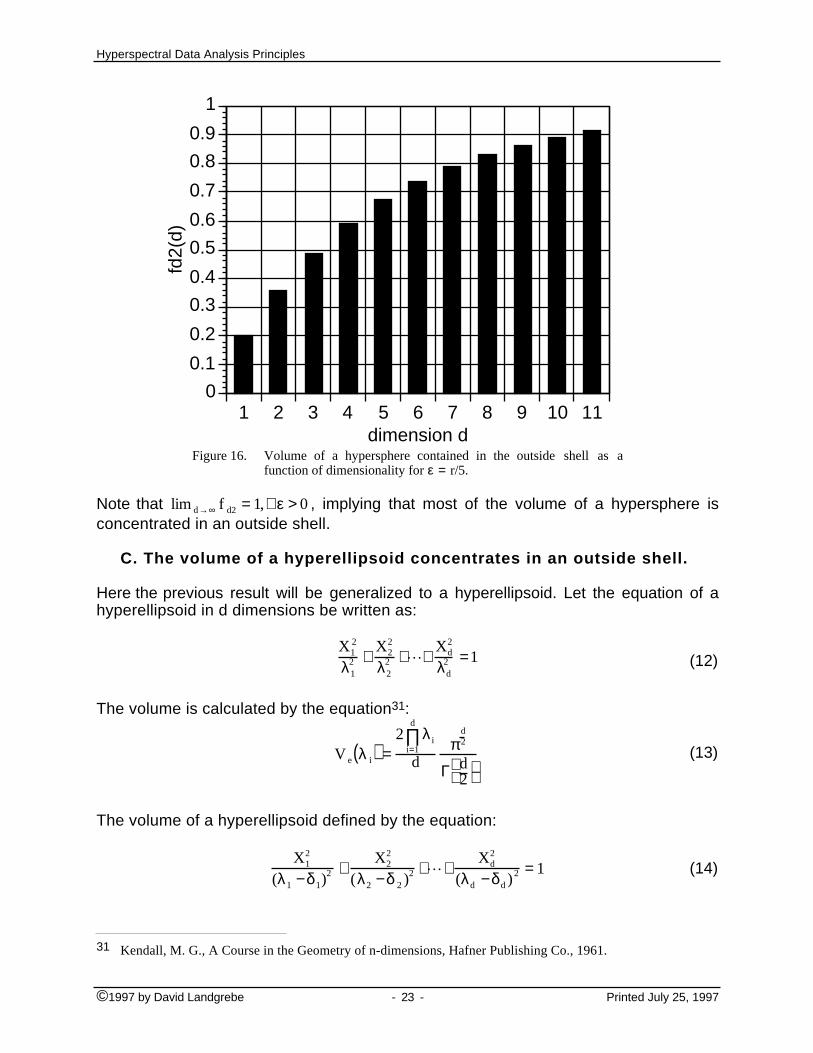
In Figure 16 observe, for the case ε = r/5, how as the dimension increases the volumeconcentrates in the outside shell.

29 Kendall, M. G., A Course in the Geometry of n-dimensions, Hafner Publishing Co., 1961.30 Wegman, E. J., "Hyperdimensional Data Analysis Using Parallel Coordinates," Journal of the American

Statistical Association, Vol. 85, No. 411, pp. 664-675, 1990



1 2 3 4 5 6 7 8 9 10 110

0.1

0.2

0.3

0.4

0.5

0.6

0.7

0.8

0.9

1

fd2(

d)

dimension dFigure 16. Volume of a hypersphere contained in the outside shell as a

function of dimensionality for ε = r/5.

Note that lim d→∞ f d2 = 1,∀ε > 0 , implying that most of the volume of a hypersphere isconcentrated in an outside shell.

C. The volume of a hyperellipsoid concentrates in an outside shell.

Here the previous result will be generalized to a hyperellipsoid. Let the equation of ahyperellipsoid in d dimensions be written as:

X12

λ12 +

X22

λ22 +L+

Xd2

λd2 =1 (12)

The volume is calculated by the equation31:

V e λ i( ) =2 λi

i=1

d

∏d

πd2

Γ d2

(13)

The volume of a hyperellipsoid defined by the equation:

X12

(λ1 −δ 1)2 +

X22

(λ2 −δ 2 )2 +L+Xd

2

(λd −δ d )2 = 1 (14)

31 Kendall, M. G., A Course in the Geometry of n-dimensions, Hafner Publishing Co., 1961.



where 0 ≤δ i < λi ,∀i , is calculated by:

V e λ i −δ i( ) =2 (λi −δ i)

i =1

d

∏d

πd2

Γ d2

(15)

The fraction of the volume of V e(λ i −δ i) inscribed in the volume V e(λ i) is:

f d3 =λi −δ i( )

i =1

d

∏

λ ii =1

d

∏= 1−

δi

λi

i =1

d

∏ (16)

Let γ min = minδ i

λ i( ) , then

f d3 = 1 −δi

λ i

i =1

d

∏ ≤ 1− γmin( )i =1

d

∏ = 1 −γ min( )d(17)

Using the fact that f d3 ≥ 0, it is concluded that limd→∞

fd3 = 0 .

The characteristics previously mentioned have two important consequences for highdimensional data that appear immediately. The first one is that

• High dimensional space is mostly empty,which implies that multivariate data in a high dimensional feature space is usually in alower dimensional structure. As a consequence high dimensional data can beprojected to a lower dimensional subspace without losing significant information interms of separability among the different statistical classes. The second consequenceof the foregoing, is that

• Normally distributed data will have a tendency to concentrate in the tails.Similarly,

• Uniformly distributed data will be more likely to be collected in the corners,making density estimation more difficult. Local neighborhoods are almost surelyempty, requiring the bandwidth of estimation to be large and producing the effect oflosing detailed density estimation.

Support for this tendency can be found in the statistical behavior of normally anduniformly distributed multivariate data at high dimensionality. It is expected that as thedimensionality increases the data will concentrate in an outside shell. As the numberof dimensions increases that shell will increase its distance from the origin as well.

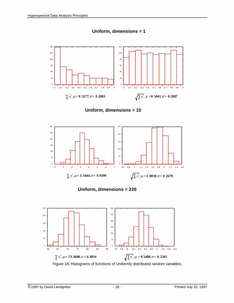
To show this specific multivariate data behavior, an experiment was developed.Multivariate normal and uniform distributed data were generated. The normal anduniform variables are independent identically distributed samples from thedistributions N(0,1) and U(-1,1), respectively. Figures 17 and 18 illustrate thehistograms of random variables, the distance from the zero coordinate and its square,that are functions of normal or uniform vectors for different number of dimensions.



Normal, dimensions = 1

0

50

100

150

200

250

300

0 0.5 1 1.5 2 2.5 3 3.5

0

100

200

300

400

500

600

700

800

0 2 4 6 8 10 12 14 16

xi2

i∑ ,µ= 1.0168,σ =1.4017 x i

2

i∑ ,µ= .7736,σ= .5737


50

100

150

200

250

300

0

0 5 10 15 20 25 30 1 1.5 2 2.5 3 3.5 4 4.5 5 5.5

0

50

100

150

200

250

6

xi2

i∑ ,µ =9.8697,σ= 4.5328 x i

2

i∑ ,µ = 3.1026,σ =0.7042


0

50

100

150

200

250

140 160 180 200 220 240 260 280 300 12 13 14 15 16 17 18

0

50

100

150

200

250

300

xi2

i∑ ,µ =220.3732,σ = 20.7862 x i

2

i∑ ,µ= 14.8497,σ = 0.7129

Figure 17. Histograms of functions of Normally distributed random variables.



Uniform, dimensions = 1

xi2

i∑ ,µ= 0.3277,σ= 0.2883 x i

2

i∑ ,µ =0.5041,σ= 0.2887

0

50

100

150

200

250

300

0 0.1 0.2 0.3 0.4 0.5 0.6 0.7 0.8 0.9 1

0

20

40

60

80

100

120

0 0.1 0.2 0.3 0.4 0.5 0.6 0.7 0.8 0.9 1


xi2

i∑ ,µ= 3.3444,σ= 0.9390 x i

2

i∑ ,µ =1.8010, σ= 0.2678

0

50

100

150

200

250

300

0 1 2 3 4 5 6 7

0

50

100

150

200

250

0.6 0.8 1 1.2 1.4 1.6 1.8 2 2.2 2.4 2.6


x i2

i∑ ,µ= 73.3698,σ = 4.3854 x i

2

i∑ ,µ = 8.5488,σ= 0.2505

0

50

100

150

200

250

60 65 70 75 80 85 90

0

50

100

150

200

250

300

7.6 7.8 8 8.2 8.4 8.6 8.8 9 9.2 9.4 9.6

Figure 18. Histograms of functions of Uniformly distributed random variables.



These experiments show how the means and the standard deviations are functions ofthe number of dimensions. As the dimensionality increases, the data concentrates inan outside shell. The mean and standard deviation of two random variables,

r = x i

2

i =1

d

∑ and R = x i

2

i =1

d

∑are computed. These variables are the distance and the square of the Euclideandistance of the random vectors. The values of the parameters and the histograms ofthe random variables are shown in Figure 16 and 17 for normal and uniformdistribution of the data. As the dimensionality increases, the distance from the zerocoordinate of both random variables increases as well. These results show that thedata have a tendency to concentrate in an outside shell and how the shell's distancefrom the zero coordinate increases with the increment of the number of dimensions.

Note that R = x i

2

i =1

d

∑ has a chi-square distribution with d degrees of freedom when the

xi's are samples from the N(0,1) distribution. The mean and variance of R are32: E(R) =d, Var(R) = 2d . This conclusion supports the previous thesis.

Under these circumstances it would be difficult to implement any density estimationprocedure and obtain accurate results. Generally nonparametric approaches will haveeven greater problems with high dimensional data.

D. The diagonals are nearly orthogonal to all coordinate axes33,34

The cosine of the angle between any diagonal vector and a Euclidean coordinate axisis:

cos θd( ) =± 1d

,

Figure 19 illustrates how the angle between the diagonal and the coordinates, θd ,approaches 90o with increases in dimensionality.

32 Scharf, L. L. "Statistical Signal Processing. Detection, Estimation, and Time Series Analysis." Massachusetts:Addison-Wesley, 1991.

33 Scott, D. W. "Multivariate Density Estimation." John Wiley & Sons, pp. 27-31, 1992.34 Wegman, E. J., "Hyperdimensional Data Analysis Using Parallel Coordinates," Journal of the American

Statistical Association, Vol. 85, No. 411, 1990



Figure 19. Angle (in degrees) between a diagonal and a Euclidean coordinate vs.dimensionality.

Note that lim d→∞ cos θd( ) = 0 , which implies that in high dimensional space thediagonals have a tendency to become orthogonal to the Euclidean coordinates.

This result is important because,

• The projection of any cluster onto any diagonal, e.g., by averaging features,could destroy information contained in multispectral data.

In order to explain this, let adiag be any diagonal in a d dimensional space. Let acibe the ith coordinate of that space. Any point in the space can be represented by theform:

P = αii=1

d

∑ aci

The projection of P over adiag, Pdiag is:

Pdiag = PTadiag( )adiag = α ii =1

d

∑ ac iT ad( )ad

But as d increases ac iTadiag ≈ 0 which implies that Pdiag ≈ 0. As a consequence Pdiag

is being projected to the zero coordinate, losing information about its location in the ddimensional space.



E. The required number of labeled samples for supervisedclassification increases as a function of dimensionality.

As previously stated, Fukunaga35, in a given circumstance, proves that the requirednumber of training samples is linearly related to the dimensionality for a linearclassifier and to the square of the dimensionality for a quadratic classifier. That fact isvery relevant, especially since experiments have demonstrated that there arecircumstances where second order statistics are more relevant than first order statisticsin discriminating among classes in high dimensional data36. In terms of nonparametricclassifiers the situation is even more severe. It has been estimated that as the numberof dimensions increases, the sample size needs to increase exponentially in order tohave an effective estimate of multivariate densities37,38.

It is reasonable to expect that high dimensional data contains more information in thesense of a capability to detect more classes with more accuracy. As a matter of fact,since the curves of Figure 12 are montonically increasing, ultimately one can expect100% accuracy, on the average. At the same time the above characteristics tell us thatcurrent techniques, which are usually based on computations at full dimensionality,may not deliver this advantage unless the available labeled data is substantial. Thiswas shown in Figure 13 where, with a limited number of training samples, there is apenalty in classification accuracy as the number of features increases beyond somepoint.

F. For most high dimensional data sets, low linear projections havethe tendency to be normal, or a combination of normal distributions,as the dimension increases.

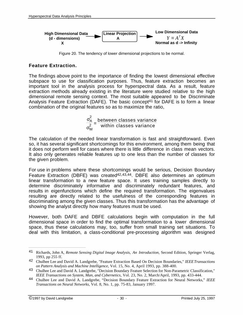
That is a significant characteristic of high dimensional data that is quite relevant to itsanalysis. It has been proved39,40 that, as the dimensionality tends to infinity, lowerdimensional linear projections will approach a normal (Gaussian) distribution withprobability approaching one (see Figure 20). Normality in this case implies a normal ora combination of normal distributions. This lends credence to using Gaussianclassifiers after having reduced the dimensionality via feature extraction and indeed, tousing class mean vectors and covariance matrices in evaluating the separability ofclasses. Properly used, parametric classifiers should provide good performance, andnonparametric schemes, with their higher demands for training data, should not beneeded.

35 Fukunaga, K. "Introduction to Statistical Pattern Recognition." San Diego, California, Academic Press, Inc.,1990.


37 Scott, D. W. "Multivariate Density Estimation." John Wiley & Sons, pp. 208-212, 1992.38 Hwang, J., Lay, S., Lippman, A., "Nonparametric Multivariate Density Estimation: A Comparative Study.",

IEEE Transactions on Signal Processing, Vol. 42, No. 10, 1994, pp. 2795-2810.39 Diaconis, P., Freedman, D. "Asymptotics of Graphical Projection Pursuit." The Annals of Statistics Vol. 12,

No 3 (1984): pp. 793-815.40 Hall, P., Li, K. "On Almost Linearity Of Low Dimensional Projections From High Dimensional Data." The

Annals of Statistics, Vol. 21, No. 2 (1993): pp. 867-889.



High Dimensional Data (d - dimensions) X

Linear Projection A

Low Dimensional Data

Normal as d -> InfinityY = ATX

Figure 20. The tendency of lower dimensional projections to be normal.

Feature Extraction.

The findings above point to the importance of finding the lowest dimensional effectivesubspace to use for classification purposes. Thus, feature extraction becomes animportant tool in the analysis process for hyperspectral data. As a result, featureextraction methods already existing in the literature were studied relative to the highdimensional remote sensing context. The most suitable appeared to be DiscriminateAnalysis Feature Extraction (DAFE). The basic concept41 for DAFE is to form a linearcombination of the original features so as to maximize the ratio,

σ2A

σ2W

= between classes variance within classes variance

The calculation of the needed linear transformation is fast and straightforward. Evenso, it has several significant shortcomings for this environment, among them being thatit does not perform well for cases where there is little difference in class mean vectors.It also only generates reliable features up to one less than the number of classes forthe given problem.

For use in problems where these shortcomings would be serious, Decision BoundaryFeature Extraction (DBFE) was created42,43,44. DBFE also determines an optimumlinear transformation to a new feature space. It uses training samples directly todetermine discriminately informative and discriminately redundant features, andresults in eigenfunctions which define the required transformation. The eigenvaluesresulting are directly related to the usefulness of the corresponding features indiscriminating among the given classes. Thus this transformation has the advantage ofshowing the analyst directly how many features must be used.

However, both DAFE and DBFE calculations begin with computation in the fulldimensional space in order to find the optimal transformation to a lower dimensionalspace, thus these calculations may, too, suffer from small training set situations. Todeal with this limitation, a class-conditional pre-processing algorithm was designed

41 Richards, John A, Remote Sensing Digital Image Analysis, An Introduction, Second Edition, Springer Verlag,1993, pp 255 ff.

42 Chulhee Lee and David A. Landgrebe, "Feature Extraction Based On Decision Boundaries," IEEE Transactionson Pattern Analysis and Machine Intelligence, Vol. 15, No. 4, April 1993, pp. 388-400.

43 Chulhee Lee and David A. Landgrebe, "Decision Boundary Feature Selection for Non-Parametric Classification,"IEEE Transactions on System, Man, and Cybernetics, Vol. 23, No. 2, March/April, 1993, pp. 433-444.

44 Chulhee Lee and David A. Landgrebe, “Decision Boundary Feature Extraction for Neural Networks,” IEEETransactions on Neural Networks, Vol. 8, No. 1, pp. 75-83, January 1997.



based upon a method known as projection pursuit45,46. This algorithm does thenecessary calculations in the projected space, rather than the original, highdimensional space. Figure 21 shows the overall scheme. The data at point Φ might be200 dimensional. Through projection pursuit, a subspace of perhaps 20 dimensionsmight be determined, and in this case, all calculations are done at a dimensionality of20. This can then more optimally be followed by DAFE or DBFE to find a subspace ofperhaps 10 dimensions in which to do the classification. In this way, maximaladvantage can be taken of a training set of limited size.

Class Conditioned Pre-processing

High Dimensional Data

Classification/AnalysisFeature Extraction

Dimension Reduced

Dimension Further Reduced

Sample Label Information

ΦΓ Ψ Ω

Figure 21. Classification of high dimensional data including reprocessing of high dimensional data.

Summary and Conclusions

What is sought are powerful, general analysis procedures that approach the optimumin information extraction capabilities and yet are within the reach of and practical for abroad range of Earth scientists and other remote sensing practitioners. The techniquesmust be 1) powerful in terms of accuracy and detail with respect to the classes whichcan be discriminated, 2) objective in their performance, 3) robust with regard to thebreadth of discipline problems which can be successfully approached, and yet 4) mustappear sound and practical to scientists with a broad set of discipline backgrounds.They must be derived with appropriate mathematical rigor, but in the end, they mustmeet the practical conditions of the randomness of the scene, noise introduced by theatmosphere, the scene, and the sensor, and the varied skills and expectations of theusers.

Summarizing to this point, the key conclusions expressed above are,

45 Luis Jimenez and David Landgrebe, “Projection Pursuit For High Dimensional Feature Reduction: Parallel AndSequential Approaches,” Presented at the International Geoscience and Remote Sensing Symposium(IGARSS'95), Florence Italy, July 10-14, 1995.

46 Luis Jimenez and David Landgrebe, “Projection Pursuit in High Dimensional Data Reduction: InitialConditions, Feature Selection and the Assumption of Normality,” IEEE International Conference on Systems,Man, and Cybernetics, Vancouver, Canada, October 22-25, 1995.



• The complexity of the scene and the dynamic nature of it is so dominant,that, except for the extraction of relatively simple information, supervision ofclassifiers must be redone for every new data set collected.

• Of the three data space presentations discussed, the feature space is themost useful for analytical purposes, though the other two are helpful forvisualization purposes.

• The typically rather uniformly distributed nature of data in feature spacemakes clear why entirely unsupervised classification schemes are not likelyto produce satisfactory results for multispectral discrimination purposes.

• A stochastic or random process approach for data modeling has beenchosen for reasons of its rigor and power, and the large stable of tools thatprove of pivotal usefulness in the work.

• Both first order variations (e.g. mean values) and second order variations(e.g. covariance matrices) are found to be significant in the discriminationprocess. On a case specific basis, either is likely to provide the mostsignificant contribution to the ability to discriminate between classes. Neithershould be ignored without good justification.

• A significant relationship has been demonstrated between the number ofspectral bands, the amount of ancillary data available for classifiersupervision, and overall classifier accuracy achievable.

• A significant relationship has also been found between classifier complexity,the amount of ancillary data available for classifier supervision, and overallclassifier accuracy achievable.

• Given these findings, a generic hierarchy of classifier algorithms has beengiven against which to judge more specialized algorithms for their likelyperformance robustness.

• A number of novel characteristics of high dimensional spaces are presentedwhich bear upon the analysis of hyperspectral data. Among them are thefacts that,- Higher dimensional spaces are mostly empty, because of the rapidity

with which volume increases with dimensionality. This suggests theimportance of feature extraction algorithms to find the lower dimensionalspace in which the most important discriminate structure exists.

- Unlike three dimensional space, data in hyperspace tends to concentratein the corners of a hypercube, in the outer shell of a hyperellipsoid, andthus in the corners of a uniform distribution and the tails of a Gaussiandistribution. This increases the importance of having adequate numbersof training samples when estimating high dimensional density functionparameters, and of using the lowest dimensionality which will providebest results.



- The diagonals in high dimensional are nearly orthogonal to allcoordinate axis. This has implications relative to averaging features.

- For most high dimensional data sets, as the dimension increases, lowerdimensional linear projections have a tendency to be normal, or acombination of normal distributions. Thus, the Gaussian assumptionbecomes better justified after feature extraction to a lower dimensionalspace.

- The required number of labeled samples for supervised classificationincreases as a function of dimensionality, and more so with increasedgenerality of the classifier algorithm used.

As a result of these findings, feature extraction algorithms assume increasedimportance, and a two stage feature extraction process has been put forth in order totake maximal advantage of the dimensionality available when, as is usually the casein the remote sensing circumstance, the number of training samples is limited.

Some of these results raise other issues with regard to current and future analysisprocedures. For example, it is seen that second order variations can be and often aremore significant than first order ones in making discrimination between classespossible. "Data correction" procedures are now common in preparing data foranalysis, but most, if not all, such procedures are directed at adjusting for first ordereffects only. Generally, the impact they might have on the second order variations in adata set have not been considered. The positive value they may have is taken on faithand has not generally been subject to study. There is some evidence47 that they maynot always have this assumed positive effect, and indeed, there effect could bedetrimental in some cases. Other such issues of this nature need also to beaddressed.

Substantial progress toward an optimal and robust hyperspectral data analysisprocedure has been made based upon the findings reported in this paper, however,some key problems remain if such a procedure is to have significant widespreadimpact. Among these are the need to,

• Make the analysis process viable for smaller and smaller training sets, downto one spectrum for some classes, while still retaining optimal characteristicsof both first and second order statistics to the extent possible. It is the casethat no one likes the idea of needing to retrain a classifier for each data set.On the other hand, the dynamic nature of the Earth's surface requires it ifmany of the more complex and challenging information extraction tasks areto be completed successfully.

• Make the analysis process systematic, making as much of the complexity ofit transparent to the user, so that it appears attractive and reasonable to theuser community. The need is to take advantage of human knowledge and

47 Joe Hoffbeck and David A. Landgrebe, “Effect Of Radiance-To-Reflectance Transformation And AtmosphereRemoval On Maximum Likelihood Classification Accuracy Of High-Dimensional Remote Sensing Data,”Proceedings of the International Geoscience and Remote Sensing Symposium (IGARSS'94), CD-ROM pp.3289-3294, Pasadena, Calif, August 8-12,1994.



perception while at the same time not requiring analysts to be highly trainedand experienced signal processing engineers.

As an example, the labeling of samples for training sets seems onerous to everyone,and unreasonable or unnecessary to some. It is certainly desirable to avoid doing thiswhenever possible. However, the more challenging information extraction problemssimply require it. There often are ways to mitigate the problem which are situationspecific in any given case. An example in a geologic survey case, making use ofchemical spectroscopy characteristics has been given48 as an illustration in onecircumstance. Any way to make this part of the analysis process acceptable to theEarth scientist or practitioner would be an important contribution to the field. It is tothese and related objectives that future research needs to be directed.

And finally, it is recognized that a key problem is to deliver the knowledge andalgorithms derived during this research to the potential users. For this purpose, anapplication program for personal computers has been created with a basicmultispectral data analysis capability and made available to the community withoutcharge. Then as new algorithms emerge from the research, they are incorporated intothe program and new versions of it issued. In this way, new algorithms, which may bequite complex to implement may be tried by users with a minimum of effort on theirpart. The program, called MultiSpec, together with substantial documentation isavailable for anyone interested to download from the world wide web. The URL for theweb site is

http://dynamo.ecn.purdue.edu/~biehl/MultiSpec/Some of the algorithms mentioned above which it now contains are, DiscriminateAnalysis Feature Extraction (DAFE), Decision Boundary Feature Extraction (DBFE),Statistics Enhancement, and Statistics Image. It also contains the spatial/spectralanalysis algorithm created some years ago called ECHO, as mentioned earlier. Thisalgorithm has proven to be easy to use, computationally efficient and effective inincreasing classification accuracy, but it is not simple to implement, and this has nodoubt inhibited its wider use.

48 Hoffbeck, Joseph P. and David A. Landgrebe, “Classification of Remote Sensing Images having High SpectralResolution,” Remote Sensing of Environment, Vol. 57, No. 3, pp. 119-126, September 1996.


on information extraction principles for hyperspectral datalandgreb/whitepaper.pdf · on...

Documents