ON-LINE SCHEDULINGAND

W.I.P. REGULATION

Jean-Marie PROTH

Production background

The production system works 24 hours a day.

When an order appears in the production system, we have to provide the best delivery time in real time to the customer (less than 3 minutes).

Previous schedule cannot be modified.

ON-LINE SCHEDULINGAND

W.I.P. REGULATION:

THE JOB-SHOP CASE

Since orders are scheduled as soon as they

appear in the system, the job-shop case is a

flow-shop for each one of the orders.

Basic problem

m operations O1, …, Om must be performed to complete a given order. Each operation is performed by one resource or several identical resources. Each resource is partially busy when the order appears in the system. We have to manufacture a product using the idle periods of the resources.

We first arrange the idle windows in the increasing order of their lower limit.

Classifying the idle periods

Three identical resources for one operation

R1

R2

R3

1

2

3

4

5

6

7

8

9

O

α1 β1

α2 β2

α3 β3

α4 β4

α5 β5

α6 β6

α7 β7

α8 β8

α9 β9

Problem setting

The operations should be performed in

the order O1, O2, …, Om.

The time spent for performing Oi, i=1, …, m

belongs to [θi, θi+δi].

Product cannot be stored between two

operations.

Objective: Minimize the completion time.

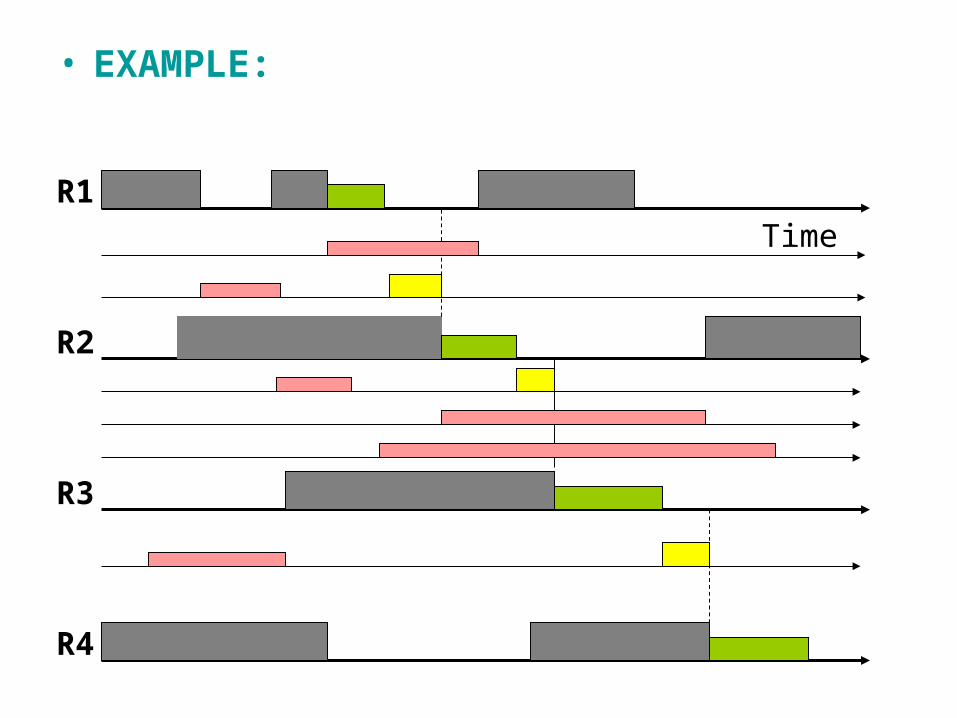
• EXAMPLE:

O1

O2

O3

O4

Time

BUSY PERIODS

MANUFACTURING TIMES EXTENSIONS OF MAN. TIMES

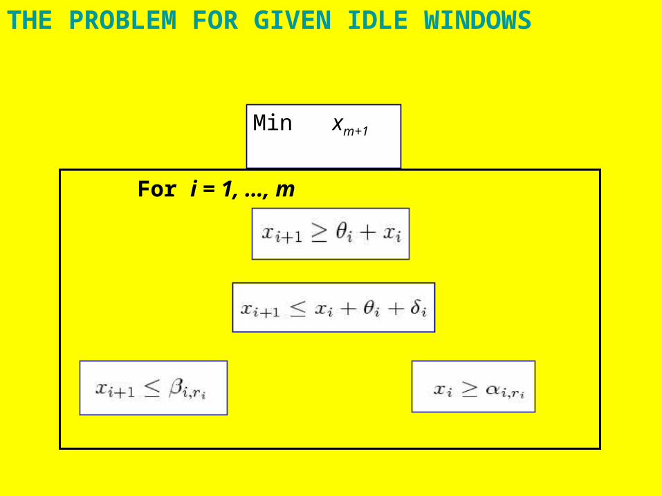
THE PROBLEM FOR GIVEN IDLE WINDOWS

Min xm+1

For i = 1, …, m

THE ALGORITHM

Do 2.3.

,...,2for ,max Do 2.2.

Do 2.1.

.,,...,, sequence theBuilding .2

m1

11,

,11

121

1

mm

iikii

k

mm

tt

mitt

t

ttttT

I

.,...,2,1for 1 Do .1 miki

1,...,1, for

,max Do 3.2.

Do .1.3

,...,, sequence theBuilding 3.

1

11

11

mmi

xtx

tx

xxxX

iiiii

mm

mm

2. step return to

weand 1set we, that

such ,...,2,1any for Otherwise, 4.2.

alg. theof End reached. is valueoptimal

then the,,...,1for If 4.1.

Test .4

,1

,1

iikii

kii

kkx

mi

mix

i

i

The ki value is the rank of the idle window in which we want to perform operation i, for i=1 to m.

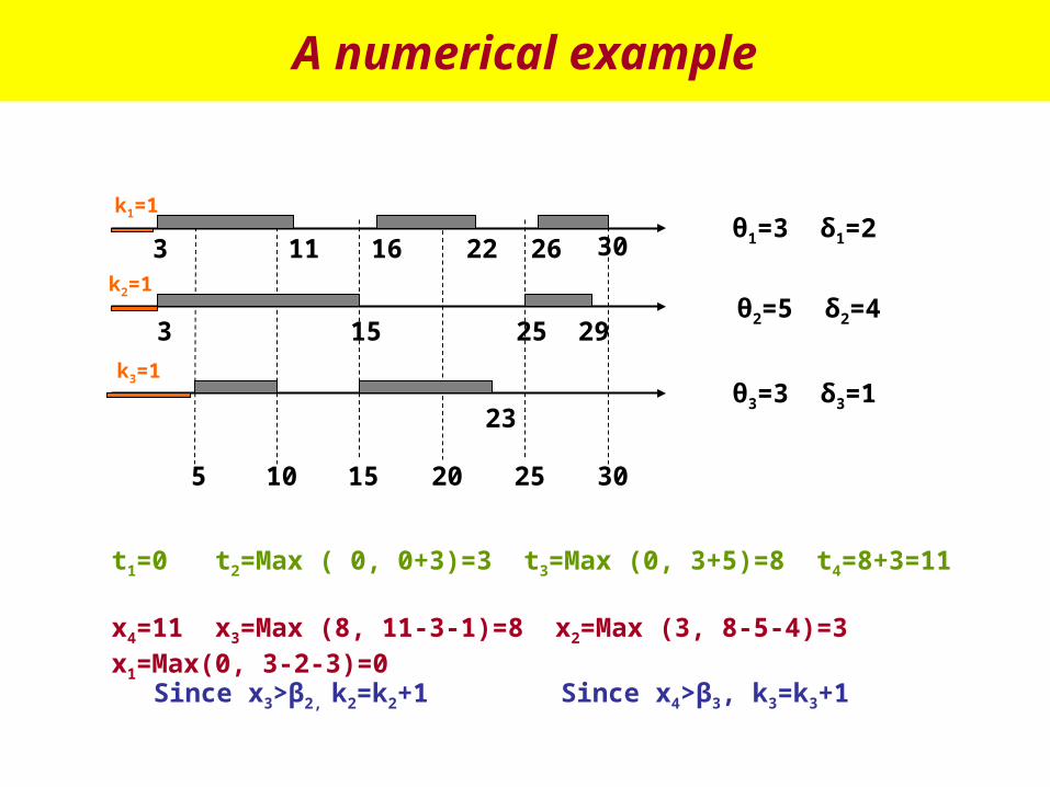
A numerical example

5 10 15 20 25 30

3 11 16 22 26 30

3 15 25 29

23

θ1=3 δ1=2

θ2=5 δ2=4

θ3=3 δ3=1

k1=1

k2=1

k3=1

t1=0 t2=Max ( 0, 0+3)=3 t3=Max (0, 3+5)=8 t4=8+3=11

x4=11 x3=Max (8, 11-3-1)=8 x2=Max (3, 8-5-4)=3 x1=Max(0, 3-2-3)=0

Since x3>β2, k2=k2+1 Since x4>β3, k3=k3+1

5 10 15 20 25 30

3 11 16 22 26 30

3 15 25 29

23

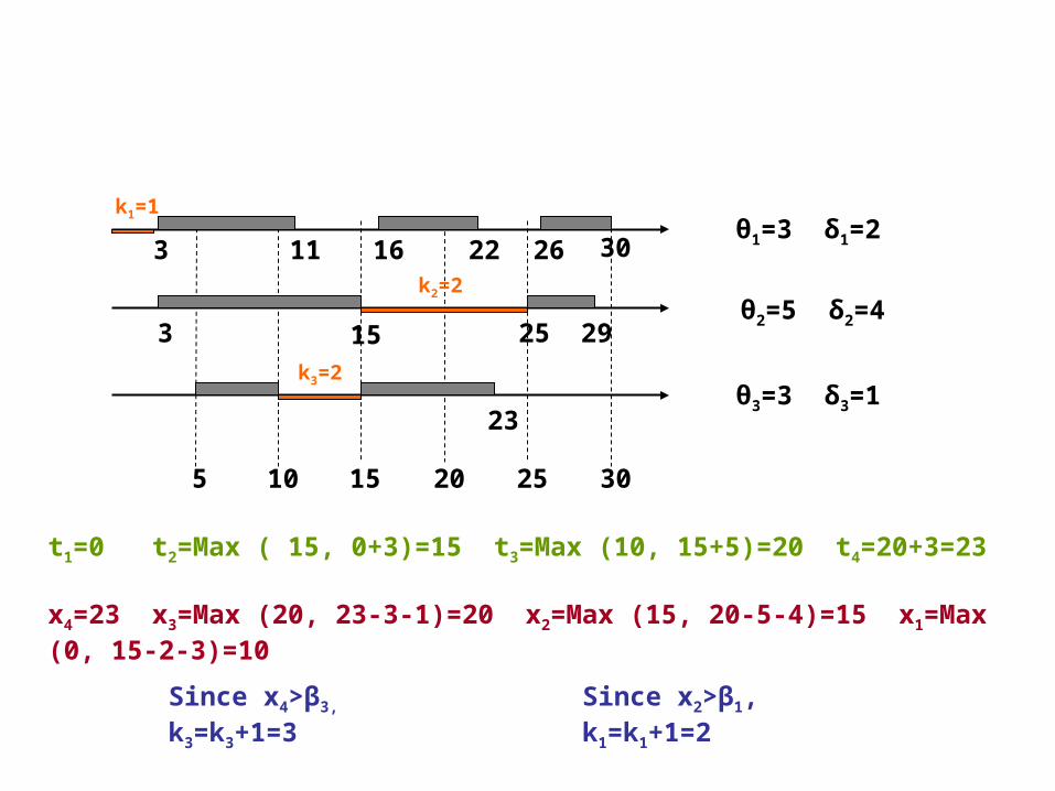
θ1=3 δ1=2

θ2=5 δ2=4

θ3=3 δ3=1

k1=1

t1=0 t2=Max ( 15, 0+3)=15 t3=Max (10, 15+5)=20 t4=20+3=23

x4=23 x3=Max (20, 23-3-1)=20 x2=Max (15, 20-5-4)=15 x1=Max (0, 15-2-3)=10

Since x4>β3, k3=k3+1=3 Since x2>β1, k1=k1+1=2

k2=2

k3=2

5 10 15 20 25 30

3 11 16 22 26 30

3 15 25 29

23

θ1=3 δ1=2

θ2=5 δ2=4

θ3=3 δ3=1

k1=2

k2=2

k3=3

t1=11 t2=Max ( 15, 11+3)=15 t3=Max (23, 15+5)=23 t4=23+3=26

x4=26 x3=Max (23, 26-3-1)=23 x2=Max (15, 23-5-4)=15 x1=Max(11, 15-2-3)=11

THIS SOLUTION IS OPTIMAL

5 10 15 20 25 30

3 11 16 22 26 30

3 15 25 29

23

θ1=3 δ1=2

θ2=5 δ2=4

θ3=3 δ3=1

THIS SOLUTION IS OPTIMAL

REMARKS

1. It is not always possible to extend the operation time.

2. A resource is busy until the end of the operation time (including its extension).

⇓We transform the extension of the

operation time into inventory time.

Two approaches are proposed:

Approach 1:

We are interested in managing only the inventory time between two operations.

Approach 2:

We are interested in managing both the inventory time and the number of parts in inventory between two operations.

APPROACH 1

We add a “storage resource” at the end of each operation.

These storage resources are totally idle each time a new order appears in the production system.

R1

R2

R3

R4

Time

BUSY PERIODS

MAN. TIMES

S1

S2

S3

STORAGE PERIODS

APPROACH 2

We add as many “storage resources” as the number of WIP units that are allowed at the exit of an operation.

We keep the busy periods of these “storage operations”.

The δi and θi are assigned as in approach 1.

• EXAMPLE:

R1

R2

R3

R4

Time

ON-LINE SCHEDULINGAND

W.I.P. REGULATION:

THE ASSEMBLY SYSTEM CASEThe algorithm for on-line scheduling and WIP management in assembly systems is based on the previous algorithm.

The idea behind this algorithm is to adjust iteratively job-shop like systems.

12

5

37

6

4

14

13

1

10 11

9

2

8

EXAMPLE

1

147

6

5S1

10 14131211S5

14743S4

8 1413129S3

2

147

6

5S2

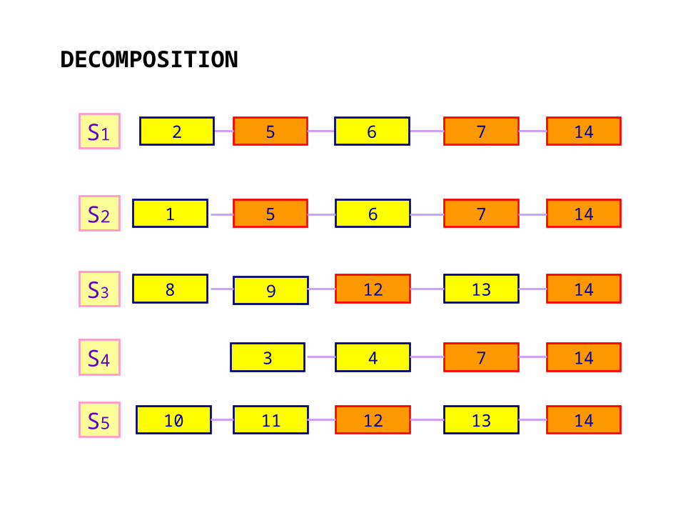
DECOMPOSITION

If we apply the job-shop algorithm to each one of the lines, there is little likelihood that a given assembly operation starts at the same time in the different schedules.

We propose an iterative approach that adjust gradually the starting time of each assembly operation. This approach is based on the two following rules.

The proposed algorithm converges to the optimal solution, i.e. to the minimal makespan.

RULE 1

In the resulting schedule:

If a given assembly operation is scheduled in different windows, we restart the computation constraining this operation to be scheduled at the earliest in the last window.

S1

S2

S4k k+1 k+2

We restart the algorithm with window k+2 in all the linesthat contain this assembly operation.

Assembly operation 7

RULE 2

In the resulting schedule:If a given assembly operation is scheduled in the same window whatever the line, then we restart the computation from this window after assigning to the lower bound of the window the greatest starting time of the operation.

Configuration when restarting the scheduling

New window