On Mean Variance Portfolio Optimization: Improving

Performance Through Better Use of Hedging Relations ∗

Shingo Goto†

University of South Carolina

Yan Xu‡

University of Rhode Island

November 2009

This version: February 2012

∗We thank Yufeng Han, Jingzhi (Jay) Huang, Steven Mann, Zhan Shi, Walter Torous, Raman Uppal, Rossen

Valkanov, Masahiro Watanabe, Hong Yan, Frank Yu, Yuzhao Zhang and Guofu Zhou for helpful comments

and discussions. This research also benefits greatly from discussions with a number of investment professionals.

We are especially grateful to Miguel Alvarez at Deutsche Bank Securities; Nick Baturin at Bloomberg; Vinod

Chandrashekaran, Hong Leng Chuah, Mohanaraman Gopalan, Daniel Morillo, Jeff Shen, and Li Wang at Black-

rock/BGI; Ernie Chow, Jonathan Howe, and Scott Shaffer at Senstato Capital Management; Julian Douglass and

Matt Kurbat at CPP Investment Board; Xiaowei Li at Fullgoal Fund Management; David Stewart at Durant

Capital Management; Dawn Jia at State Street Global Advisors; and Jim Wang at Bosera Funds. Of course all

errors and inadequacy are the authors’ own.

†Moore School of Business, University of South Carolina, 1705 College St., Columbia, SC 29208, USA; phone:

+1 803 777 6644; fax +1 803 777 6876; email: shingo.goto@moore.sc.edu.

‡College of Business Administration, University of Rhode Island; 7 Lippitt Road, Kingston, RI 02881-0802,

USA; phone: +1 401 874 4190; fax: +1 401 874 4312; email: yan xu@mail.uri.edu.

On Mean Variance Portfolio Optimization: Improving

Performance Through Better Use of Hedging Relations

Abstract

Portfolio optimization achieves risk reduction beyond naıve diversification by ex-

ploiting hedging relations among stocks. Stevens (1998) shows that the inverse

covariance matrix prescribes the hedge trades where a portfolio of stocks hedges

each one with all other stocks to minimize portfolio risk. However, in a large port-

folio of, for example, 100 stocks, using the other 99 stocks to hedge one stock is not

necessarily optimal, as it entails large estimation errors due to multicollinearity. To

improve the mean-variance portfolio optimization, we propose a method to reduce

the effects of estimation errors in the hedge trades. We introduce a sparse inverse

covariance matrix estimator, which effectively reduces the number of stocks in each

hedge trade. Many, but not all, of the inverse are zero in the proposed inverse,

meaning that each hedge trade uses only a subset of the stocks in a given portfo-

lio. Supporting our motivation, portfolios formed on the proposed estimator achieve

significant out-of-sample risk reduction in a range of empirical applications. Their

out-of-sample performance compares favorably with those under no-short-sale re-

striction (Jagannathan and Ma (2003)), using shrunk covariance matrix (e.g. Ledoit

and Wolf (2003, 2004)), and using industry factor model (Chan, karceski and Lakon-

ishok (1999)). By improving hedge trades, our approach delivers higher certainty

equivalent returns after transaction costs.

Mean variance portfolio optimization relies on covariances to transform expected returns

into optimal portfolio weights. Consider a portfolio of N stocks. A portfolio manager uses an

asset pricing model to predict a vector of expected returns, denoted by µ, and employs a risk

model to predict the covariance matrix, denoted by Σ.1 Then, it is well known that her optimal

portfolio weights are summarized by

w ∝ Σ−1µ.

In this familiar result, the inverse covariance matrix Σ−1 plays a pivotal role in transforming

the return forecast µ into the optimal portfolio weights w. Therefore, we take the liberty of

calling the inverse covariance matrix, Ψ ≡ Σ−1, the mean variance optimizer.2

While simple and forceful in theory, the idea of mean variance portfolio optimization turns

out to be surprisingly difficult to implement. In many real world situations, the available number

of historical return observations per stock (T ) is not much larger than the number of stocks

(N).3 Then, the inverse covariance matrix (the mean variance optimizer) estimated from the

sample becomes very sensitive to small perturbations in the estimated covariances, making it

unstable from one period to another. As a consequence, the mean variance optimizer tends

to produce poor out-of-sample performance. The mean variance optimization tends to erode,

rather than enhance, the gains from naıve diversification policies such as equal-weighting (e.g.,

Jobson and Korkie (1981a), DeMiguel, Garlappi, and Uppal (2009).) Michaud (1989) even calls

the mean variance optimization the “error maximization.”4

1We assume that a riskless asset exists for both borrowing and lending. Unless otherwise stated, the termstock return in this paper refers to excess return, which is calculated by subtracting the return of the risklessasset from the total return.

2Inverse covariance matrix is also called “precision matrix” or “concentration matrix” (Dempster (1972)).

3For example, consider an active manager who runs a number of portfolios based on her proprietary sourcesof information (“signals”). Each signal portfolio tends not to have a large number of historical returns.

4Please see Brandt (2009) for a comprehensive review of the literature.

1

To regain our confidence in the mean variance optimization framework, we propose an im-

provement of the mean variance optimizer Ψ = Σ−1. In principle, the mean variance optimizer

achieves risk reduction beyond naıve diversification by hedging relations among stocks. Specifi-

cally, since stock returns are correlated, we can use each stock to hedge others. Motivated by this

simple idea, our proposed estimator of Ψ = Σ−1 delivers a significant portfolio risk reduction

out-of-sample. Our approach has three features that are different from previous contributions.

First, our motivation to enhance the hedging relations among stocks differentiates us from

many existing papers that start from assuming a structure on the return generating process

(e.g., linear factor model). To elaborate, Stevens (1998) shows that the inverse covariance

matrix of stock returns reveals the optimal hedging trades among stocks. Specifically, the i-th

row (or column) of Ψ is proportional to the stock’s minimum variance hedge portfolio. The

hedge portfolio consists of a long position in the i-th stock, and a short position in the “tracking

portfolio” of the other N − 1 stocks to hedge the i-th stock. We aim to enhance the mean

variance optimizer Ψ = Σ−1 by improving each hedge portfolio.

Second, we focus on estimating the inverse covariance matrix Ψ = Σ−1 by directly imposing

a structure on itself, rather than on the covariance matrix Σ first then inverting as existing

approaches do. For example, Chan, Karceski, and Lakonishok (1999) use a low dimensional

factor structure on the covariance matrix to improve the optimized portfolio’s out-of-sample

performance.5 Many commercial risk models (e.g. APT, Axioma, MSCI Barra, Northfield,

etc.) also appear to impose multivariate factor structures on the covariance matrix, though

their model details are proprietary and unknown.6 Ledoit and Wolf (2003, 2004a,b) shrink

5Fan, Fan, and Lv (2008) also report the advantage of employing a factor structure in optimal portfolioconstruction.

6There is also a voluminous work in the area of “robust portfolio optimization” with emphasis on the optimiza-tion process, especially from practitioners’ perspectives. Please see Fabozzi, Kolm, Pachamanova, and Focardi

2

the sample covariance matrix toward a more parsimonious target matrix, such as a constant

correlation matrix or a covariance matrix with a one factor structure. In contrast to them, our

approach applies an Occam’s razor to the inverse covariance matrix (mean variance optimizer)

Ψ = Σ−1, rather than to the covariance matrix Σ.

Third, our Occam’s razor promotes sparsity of Ψ = Σ−1. That is, our estimation method-

ology drives some of the off-diagonal elements of Ψ to zero, and these zero elements indeed

constitute a significant fraction of our estimator in empirical applications. Note that the spar-

sity of Ψ implies neither the sparsity of the covariance matrix Σ ≡ Ψ−1 nor the sparsity of the

optimal portfolio weights.7 It generally utilizes most stocks in the portfolio.

Our proposed estimator belongs to a wide class of shrinkage estimators, in that we bias

(shrink) the estimator in a direction to reduce estimation errors. However, the gains from

reducing estimation errors outweigh the costs of deviating from the optimal hedge suggested

by the past evidence. For example, each hedge portfolio is supposed to hedge one stock with

the other N − 1. But do we really need to use all the remaining N − 1 stocks? Does the fact

that the i-th and j-th stocks hedge each other strongly in the sample period imply that this

particular hedging relationship will remain in the future? With finite samples, these questions

are very difficult to answer. In this situation, we do not shy away from choosing a biased answer

– less hedging than the data suggests, or even no hedging – because such a solution reduces the

magnitude of estimation errors. As we show, our estimator of Ψ = Σ−1 is typically sparse in

empirical applications, meaning that each hedge portfolio includes only a subset of the stocks

in a given portfolio.

(2007) for a review. However, our approach is quite distinct from this venue of research.

7For example, a diagonal Ψ is sparse because all of its off-diagonal elements are zero. In this extreme case,for global minimum variance portfolio, each portfolio weight is the diagonal element itself thus non-zero.

3

To promote shrinkage and sparsity, we estimate Ψ by maximum likelihood with an addi-

tional constraint on the sum of the absolute values (i.e., l1 norm) of its off-diagonal elements.8

Intuitively, this estimation methodology works as follows: The constraint imposes a penalty on

the absolute quantities of the hedge trades, thus shrinking their overall trade size. Meanwhile,

different stocks compete with each other to enter the hedged portfolios. The methodology turns

off the j-th stock in the i-th hedged portfolio if the marginal gain from retaining the stock is

not worth the cost. This is called the “soft thresholding”. In effect, this approach restricts

the (i, j)th and (j, i)th elements of the inverse covariance matrix to be zero. In this way, we

encourage shrinkage and sparsity simultaneously in the estimation of Ψ.

Aiming for risk reduction, we test examine the out-of-sample performance of the proposed

sparse mean variance optimizer using a few representative datasets in the US and international

stock markets. Our datasets include portfolios available on Ken French’s webpage, and 100

portfolios of randomly selected 100 individual stocks from the NYSE/AMEX universe. The

proposed estimator of the mean variance optimizer accomplishes a substantial reduction in the

out-of-sample risk of the global minimum variance portfolio compared to the one based on the

sample covariance matrix. Empirically, the proposed estimator also compares favorably with

the portfolio with no-short-sale restriction (Jagannathan and Ma (2003)) and with the portfolio

based on the shrinkage covariance matrix estimator of Ledoit and Wolf (2004a). The proposed

also dominates industry factor models in improving portfolio performance of individual stocks.

The relative strength of our proposed estimator is more prominent in datasets with a large

number of assets per periods, N/T . The optimizer produces stable portfolio weights even when

8We follow Yuan and Lin (2007) and Rothman, Bickel, Levina, and Zhu (2008) in setting up the likelihoodfunction with the penalty, and employ the “glasso” algorithm of Friedman, Hastie, and Tibshirani (2008) to solvethe estimation problem.

4

N/T exceeds one, that is, when the sample covariance matrix is not invertible. The reduction in

the portfolio risk is also accompanied by a high and stable level of Sharpe ratios and certainty

equivalent returns. For many datasets, the proposed estimator of the inverse covariance matrix

Ψ delivers positive gains in certainty equivalent returns after accounting for transaction costs.

Furthermore, with the improved optimizer Ψ in place, no-short-sale constraint no longer helps

improve the out-of-sample portfolio performance. Consistent with Green and Hollifield (1992),

by improving hedge trades, Ψ helps achieve further portfolio risk reduction beyond the no-short-

sale constraint.

The rest of this paper is structured as follows. Section I. elaborates on Stevens’ (1998)

framework to motivate our approach. Section II. proposes an improved estimator of Ψ. After

setting up the out-of-sample portfolio analysis in Section III., Section IV. presents evidence on

its out-of-sample performance. Section V. concludes.

I. The Role of Hedging in Portfolio Risk Minimization

In order to motivate our approach, we first discuss the role of hedge portfolios in mean variance

portfolio optimization. Stevens (1998) shows that the inverse covariance matrix Σ−1 reveals

the optimal hedging relations among stocks. Specifically, the i-th row (or column) of Σ−1 is

proportional to the i-th stock’s hedge portfolio. The i-th hedge portfolio consists of taking (1)

a long position in i-th stock and (2) a short position in a portfolio of the other N − 1 stocks

that tracks the i-th stock return. Each tracking portfolio can be estimated from the following

regression:

ri,t = αi +

N∑k=1,k 6=i

βi|krk,t + εi,t, (1)

5

where ri,t denotes the i-th stock return in period t. εi,t is the unhedgeable component of ri,t,

whose variance is denoted by υi = V ar (εi,t). υi is a measure of the i-th stock’s unhedgeable

risk. The objective of each hedge regression is to minimize υi, and consequently, we can view

(1) as an OLS estimation problem. Stevens (1998) calls this a “regression hedge.” When βi|j is

different from zero in population, it implies that the j-th stock provides a greater hedge for the

i-th stock beyond the effects of other N − 2 stocks in the portfolio.

Let us denote the N×N covariance matrix and its inverse by Σ and define Ψ = Σ−1 =[ψij],

with ψij as the (i, j)th element. Then, Stevens (1998) establishes the following identity between

Ψ and the hedge regression (1):9

ψij =

−βi|j

υiif i 6= j

1υi

if i = j

. (2)

Remember that the hedge coefficient βi|j represents the ability of the j-th stock to hedge the

i-th stock beyond the effects of other N − 2 stocks. We can view ψij as a measure of marginal

hedgeability between the i-th and j-th stocks conditional on the presence of all other stocks in

the portfolio.10 If the i-th and j-th stocks are uncorrelated with each other after controlling for

all other stocks, then βi|j = 0 and hence ψij = 0 must hold.

We can gain more useful insights about the inverse covariance matrix by looking at its i-th

row:

Ψ (i, ·) =1

υi

[−βi|1, ...,−βi|i−1, 1,−βi|i+1, ...,−βi|N

]. (3)

9For the symmetry ψij = ψji, see Stevens’ (1998) footnote 3.

10Much earlier in the statistics literature, Dempster (1972) shows that ψij represents the conditional dependencebetween the i-th variable and the j-th variable given all other variables in the system.

6

The identity (2) and the expression for the hedge portfolio holdings (3) form the basis for

subsequent analysis.

We can regard (3) as a vector of stock holdings in the i-th stock’s hedge portfolio. It involves

a unit long position in the i-th stock and a short position of the hedge portfolio constructed

from the regression (1). The hedge portfolio is a long/short portfolio whose holdings do not

necessarily sum to a prefixed value (e.g. one). However, holdings of each asset are scaled by

1/υi, meaning that the portfolio takes a larger (smaller) position in a stock when its unhedgeable

risk is smaller (larger). We call Ψ the mean variance optimizer because it provides a detailed

prescription about the hedging trades we need to make to minimize the portfolio risk.

II. An Improved Mean Variance Optimizer

A. Objective

The framework laid out in section I. is useful to understand the sources of potential large esti-

mation errors in mean variance portfolio optimization. As shown above, each hedge regression

(1) contains a constant and N − 1 stock returns as regressors. However, many of these stock

returns are highly correlated. Furthermore, in many practical applications, the number of avail-

able historical returns to estimate the regression is not much larger than the number of stocks.

Therefore, estimation of the hedge regression with practical sample size subjects us to the econo-

metric problem: multicollinearity.11 The undesirable consequences of multicollinearity are that

the estimated hedge coefficients (β’s) have such large estimation errors that the estimates are

unstable from sample to sample, and hence too unreliable to be useful. By the identity (2), this

11Please see Judge, Griffiths, Hill, Lutkepohl, and Lee (1980) , Chapter 12, for a detailed discussion of multi-collinearity.

7

also implies that the off-diagonal elements of Ψ are also susceptible to large estimation errors

and instability.

We conquer the multicollinearity problem in two ways.12 First, in the hedged portfolio of a

stock, we shrink the portfolio holdings of other stocks. The fact that the i-th and j-th stocks

hedge each other in the past is not necessarily indicative of a continued mutual hedging relation

going forward. In the presence of this uncertainty, we prefer erring on the non-hedging side,

because it reduces the estimation errors. From the identity (2), this is equivalent to shrinking

the off-diagonal elements of the inverse covariance matrix. The rationale behind the shrinkage

is well known: an interior optimum exists in the trade-off between bias and estimation error if

our objective is to minimize the forecast error variances. On the one hand, shrinkage introduces

biases in the optimal weights of a hedge portfolio; on the other hand, it reduces the estimation

errors in the estimated portfolio weights. For proper levels of shrinkage, gains from the reduction

of estimation errors dominate the costs of biases.

Secondly, our estimation method curbs the multicollinearity more directly by just turning off

stocks that are not worth including in the hedge portfolio. In other words, our method restricts

some of the hedge portfolio weights to zero, which is equivalent to imposing zero restrictions on

the off-diagonal elements of Ψ. This corresponds to a strong form of shrinkage. When (i, j)-th

element of Ψ is zero, it simply means that the i-th and j-th stocks do not help hedge each other

in the presence of other N − 2 stocks in the portfolio. For example, when N stock returns are

driven by a small number of common factors, we may not need to use all stocks to hedge each

other.

12An alternative solution to mitigate the multicollinearity problem is to increase the number of historicalreturns (T ). For example, Jagannathan and Ma (2003) report a significant gain from using daily returns, insteadof monthly returns, to estimate the sample covariance matrix. However, in practical applications, decision makersare often constrained by the available number of historical returns.

8

In statistical literature, such a solution is called ‘lasso’ (Tibshirani, 1996). Specifically, the

shrunk parameters from hedge regression in the (1) have the following relationship with those

obtained from an OLS regression:

βi|k = sign(βOLS

i|k

)(∣∣∣βOLSi|k

∣∣∣− γ)+

where (x)+ = max(x, 0), βOLS

i|k is the full set of least square estimates, and γ is a certain soft

threshold determined by the tuning parameter. Clearly, when the magnitude of an OLS point

estimate is below the soft threshold, βi|k is set to zero. Consequently, (i, j)-th element of Ψ is

set to zero. When the absolute value of an OLS point estimate is above the soft threshold, its

sign will be given to that of βi|k, however the magnitude of βi|k is shrunk by the magnitude of

the soft threshold.

The zero restriction may again introduce potential misspecification biases (omitted regressors

in hedge regressions), but it leads to lower estimation errors. In this way, we promote the sparsity

of the mean variance optimizer Ψ = Σ−1. Needless to say, it does not imply the sparsity of the

covariance matrix Σ ≡ Ψ−1 since all stock returns are still correlated with each other. As a

matter of fact, Σ is hardly sparse even when Ψ is sparse.

B. Relation to the Recent Literature

The trade-off between the misspecification biases and estimation errors has been emphasized

in a few recent papers. For example, Jagannathan and Ma (2003) demonstrate that “wrong

constraints” (leading to misspecifications) can help improve the out-of-sample performance of

optimized portfolios to the extent that they reduce estimation errors. Ledoit and Wolf’s (2003,

2004a,b) main impetus for shrinking the sample covariance matrix is also to strike an optimal

9

balance between the misspecification biases and the estimation errors. Our approach shares the

same objective, but suggests a different route to achieve it.

An oft-cited criticism against mean variance optimization is that optimized portfolios often

involve extreme and unstable weights. Green and Hollifield (1992) argue that the extreme

weights are due to the presence of a dominant systematic factor (i.e., the market factor) in the

covariance structure: large long and short positions are unavoidable to hedge the systematic

risk regardless of the estimation errors. In response, Jagannathan and Ma (2003) demonstrate

that the measurement errors in the estimated covariance matrix still play a prominent role in

deteriorating the portfolio performance, as imposing no-short-sale constraint – that is “wrong”

in population – can improve the portfolio performance by curtailing estimation errors. Our

estimator of Ψ = Σ−1 combines some of the salient features in both papers. First, it focuses

on reducing estimation errors by promoting the parsimony of Ψ. Second, it aims to capture

the hedging relations better, so that it aids the portfolio to achieve a better hedging of the

systematic risk.

In a recent contribution, DeMiguel, Garlappi, Nogales, and Uppal (2009) (“DGNU” for

short) propose a general framework to constrain the norms of the final weighting solutions.

Their general and flexible framework encompasses many existing portfolio weighting methods,

including those of Jagannathan and Ma (2003) and Ledoit and Wolf (2003, 2004a,b). While we

believe DGNU sets a new stage in the portfolio optimization literature, we also feel that it is

worthwhile to step back to reexamine the key input (Ψ = Σ−1) for portfolio optimization. From

a practical perspective, constraining the norms of the portfolio weights is interpreted as using

a prior on the weighting solution (output) as DGNU note, but most portfolio managers acquire

and process information about the inputs rather than the outputs.

10

Furthermore, hedging relations among stocks are not necessarily stable, and portfolio man-

agers may choose to rely on their priors in choosing inputs under certain market conditions.

For example, it is known that hedging relations among various style factors, such as size and

value, have undergone substantial shifts periodically.13 With such shifts, historical covariance

provides less useful guidance, but some portfolio managers are more adept at predicting the op-

timal hedging relations among the factors. Our approach provides more flexibility to portfolio

managers as they can revise the elements of Ψ = Σ−1 to better reflect their private information

when necessary. This is possible because our approach makes the relationship between hedging

relations and optimal portfolio weights transparent.

Needless to say, out-of-sample performance of the optimized portfolios depends not only on

the optimizer Ψ = Σ−1, but also on the expected return forecast µ. Given the well-known perils

of using sample means, expected return µ should further depend on an asset pricing model

and the manager’s private information.14 Since there is a one-to-one mapping between (w,Ψ)

and (µ,Ψ), Tu and Zhou (2009a) ? propose to build economic objectives into the prior on

portfolio weights w rather than on µ. This provides a sensible approach when accompanied by

an informative input (or prior) for Ψ. Meanwhile, the success of this approach hinges on the

quality of Ψ, as the optimal weighting solution is susceptible to estimation errors in Ψ. Our focus

is on the significance of improving Ψ independent of the choice of µ, as an improved estimator of

Ψ should complement recent innovations in the literature. Consequently, we leave the problem

of finding an optimal input of µ outside the scope of this study. In empirical applications, our

13For example, rolling correlations among the Market, SMB, and HML factor returns have alternated signsbetween strongly negative and strongly positive.

14To improve the quality of µ, recent literature incorporates various theoretical restrictions in a prior distribu-tion of from a Bayesian perspective. Seminal works include Black and Litterman (1992) , Pastor (2000), Pastorand Stambaugh (2000), and MacKinlay and Pastor (2000).

11

primary focus is on the out-of-sample portfolio risk reduction of the global minimum variance

portfolio.

Nevertheless, the importance of improving the mean variance optimizer Ψ should not be

understated. While there is a general perception that estimation error in µ is far more costly

than the estimation error in Ψ, Kan and Zhou (2007) demonstrate that when N/T is not so

small, there is a very significant interactive effect between the estimation errors in µ and Ψ that

can make the optimized portfolios very unstable and unreliable.15 This is the situation in which

a stable optimizer is particularly called for. It is thus of our interest to see if our our estimator

of Ψ = Σ−1 achieves a significant reduction in the out-of-sample portfolio risk when N/T is

large.

C. Empirical Implementation

The two solutions we propose – (i) shrinkage and (ii) selection of stocks in each hedge regres-

sion – are not incompatible. We now have a statistical technology to address both objectives

simultaneously in a parsimonious manner: the least absolute shrinkage and selection operator

(lasso) (Tibshirani (1996)). They key innovation of lasso is to constrain the l1 norm of the

parameters that need to be estimated. To take advantage of this innovation, we estimate the

inverse covariance matrix Ψ directly by maximum likelihood, but with a constraint on the l1

norm of its off-diagonal elements.16

15See Chan, Karceski, and Lakonishok (1999), Jagannathan and Ma (2003), Ledoit and Wolf (2003, 2004a),among others, for similar perspectives. Kan and Zhou (2007) and Tu and Zhou (2009b) theoretically demonstratethat, in the presence of estimation errors, mean variance investors should allocate a significant fraction of wealthto the global minimum variance portfolio and equal weighted portfolio when N/T is large.

16Lasso has been receiving attention in recent econometrics literature. Caner (2009) studies a lasso-typeestimator which is formed by the GMM objective function with the addition of a penalty term. He shows thatthe lasso-type GMM correctly selects the true model much more often than other regular procedures. Bai andNg (2008) consider lasso to perform selection and shrinkage simultaneously in factor forecasting of time series .

12

Let Rt = (r1,t, . . . , rN,t)′ be a vector of N excess stock returns at time t. We consider a

problem of estimating the inverse covariance matrix Ψ from a sample of T historical observa-

tions of Rt. Put differently, T specifies the length of the “estimation window.” Rt denotes the

“centered” vector of Rt, whose elements have zero time-series means in the estimation window.17

Then, the log likelihood for the inverse covariance matrix Ψ = Σ−1 in the estimation window is

T

2ln |Ψ| − 1

2

T∑l=1

R′t−l+1ΨRt−l+1. (4)

We seek an estimator Ψ that maximizes the likelihood function (4) subject to the following

constraint: ∑N

i=1

∑N

j=1i 6=j

∣∣ψij∣∣ ≤ τ , (5)

where τ ≥ 0 is a tuning parameter so that the sum of∣∣ψij∣∣ (across all i and j, i 6= j) must be less

than or equal to τ . Expression (5) constrains the sum of the absolute values of its off-diagonal

elements, ψij (i 6= j) . In other words, we constrain the l1 norm of the off-diagonal elements of

the inverse covariance matrix Ψ.18

Intuitively, the constraint (5) promotes the overall shrinkage by restricting the sum of∣∣ψij∣∣ .

Meanwhile, it imposes the restriction of the form∣∣ψij∣∣ = 0 in the following way. Under the

constraint (5), different elements of ψij compete with each other to remain non-zero. However,

if the marginal gain from retaining the j-th stock in the i-th stock’s hedged portfolio does

not justify the cost, then we turn off the j-th stock in the i-th hedged portfolio. Then, by

the identity (2) and symmetry, this effectively restricts the (i, j)th and (j, i)th elements of the

17The MLE estimator of the mean is always the sample mean.

18Yuan and Lin (2007) and Rothman, Bickel, Levina, and Zhu (2008) solve this estimation problem in adifferent setup (graphical model).

13

inverse covariance matrix to be zero.

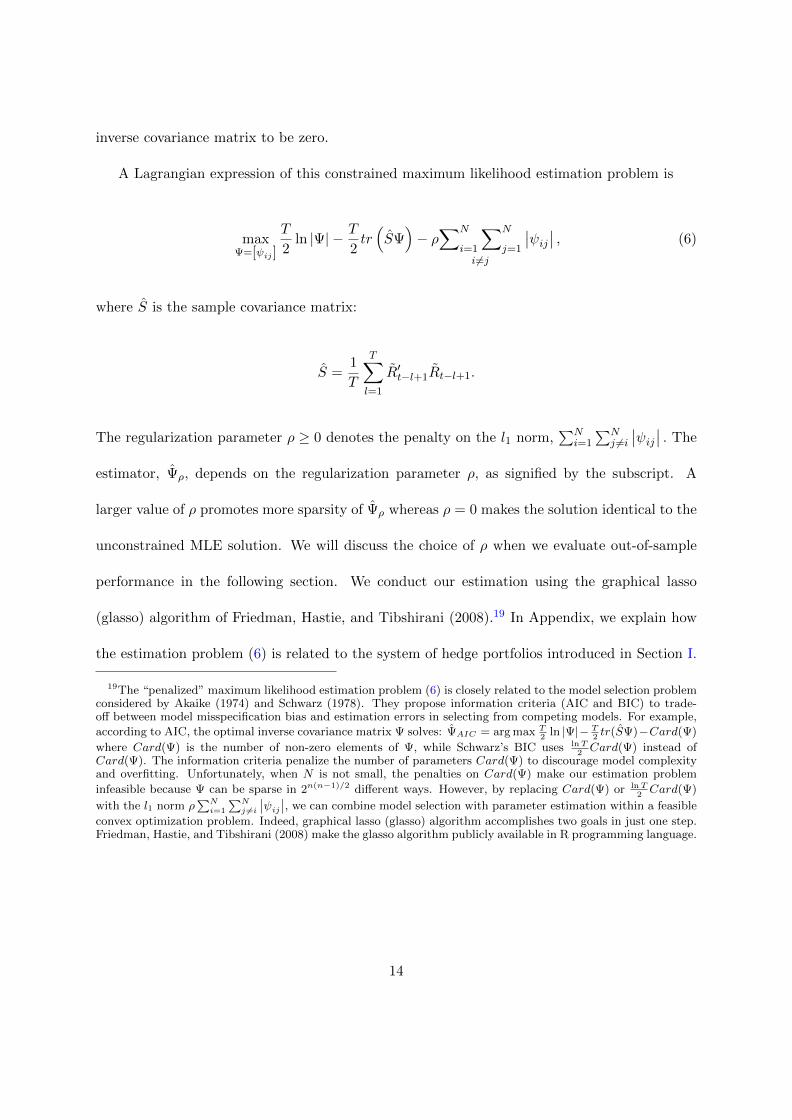
A Lagrangian expression of this constrained maximum likelihood estimation problem is

maxΨ=[ψij]

T

2ln |Ψ| − T

2tr(SΨ)− ρ∑N

i=1

∑N

j=1i 6=j

∣∣ψij∣∣ , (6)

where S is the sample covariance matrix:

S =1

T

T∑l=1

R′t−l+1Rt−l+1.

The regularization parameter ρ ≥ 0 denotes the penalty on the l1 norm,∑N

i=1

∑Nj 6=i∣∣ψij∣∣ . The

estimator, Ψρ, depends on the regularization parameter ρ, as signified by the subscript. A

larger value of ρ promotes more sparsity of Ψρ whereas ρ = 0 makes the solution identical to the

unconstrained MLE solution. We will discuss the choice of ρ when we evaluate out-of-sample

performance in the following section. We conduct our estimation using the graphical lasso

(glasso) algorithm of Friedman, Hastie, and Tibshirani (2008).19 In Appendix, we explain how

the estimation problem (6) is related to the system of hedge portfolios introduced in Section I.

19The “penalized” maximum likelihood estimation problem (6) is closely related to the model selection problemconsidered by Akaike (1974) and Schwarz (1978). They propose information criteria (AIC and BIC) to trade-off between model misspecification bias and estimation errors in selecting from competing models. For example,

according to AIC, the optimal inverse covariance matrix Ψ solves: ΨAIC = arg max T2

ln |Ψ|− T2tr(SΨ)−Card(Ψ)

where Card(Ψ) is the number of non-zero elements of Ψ, while Schwarz’s BIC uses lnT2Card(Ψ) instead of

Card(Ψ). The information criteria penalize the number of parameters Card(Ψ) to discourage model complexityand overfitting. Unfortunately, when N is not small, the penalties on Card(Ψ) make our estimation problem

infeasible because Ψ can be sparse in 2n(n−1)/2 different ways. However, by replacing Card(Ψ) or lnT2Card(Ψ)

with the l1 norm ρ∑Ni=1

∑Nj 6=i

∣∣ψij∣∣, we can combine model selection with parameter estimation within a feasible

convex optimization problem. Indeed, graphical lasso (glasso) algorithm accomplishes two goals in just one step.Friedman, Hastie, and Tibshirani (2008) make the glasso algorithm publicly available in R programming language.

14

III. Out-of-Sample Evaluation: Setup

A. Dataset and Methodology

To test the out-of-sample performance of the proposed mean variance optimizer, Ψρ, we employ

the following datasets listed in Table 1. First, the datasets cover the representative portfolios,

both US and international, that are of interest to both academic researchers and industry

practitioners. They can be classified as: portfolios formed on size and book-to-market ratio

(#1,2), industry portfolios (#3,4), country market indexes (#7,10), value and growth portfolios

in international markets (#8), and their combinations (#5,6,9). The number of assets ranges

between 15 and 148.20 Because we are interested in cases in which N/T is not small, our datasets

have more assets than those studied by DeMiguel, Garlappi, Nogales, and Uppal (2009) and

Tu and Zhou (2009a,b). Second, following Jagannathan and Ma (2003), we extract individual

stocks from AMEX and NYSE with stock price no less than 5 dollars, and with previous 120

months price record available. In order for our results not to be decided purely by a certain

combination of some individual stocks, we randomly choose 100 individual stocks at a time for

100 times, and report the average results in the following tables.

Table 1 about here.

We primarily focus on the out-of-sample performance of the minimum variance portfolio

of risky assets (stocks). Since the minimum variance locus must be constructed from risky

assets only and without risk-free ones, this portfolio also requires full initial investments. We

thus exclude any “spread assets” such as the SMB and HML factor portfolios and futures

contracts, otherwise they will allow investors to obtain risky exposure without making initial

20We thank Ken French for making many of the datasets available.

15

investments (except margins). Then spread assets won’t have bona fide returns unless we further

assume that they are covered by risk-free assets, a contradiction with above. Therefore, our

out-of-sample analysis excludes spread assets and imposes the usual constraint 1′Nw = 1, where

1N denotes the N × 1 vector of ones.21

We evaluate the out-of-sample portfolio performance using the standard “rolling-horizon”

approach. In each month t, we construct the global minimum variance portfolios using the past

120 months (10 years) of stock returns (the “estimation window,” T = 120). Next, we hold such

portfolios for one month and calculate the portfolio returns in month t + 1 out-of-sample. We

continue this process by adding the return for the next period in the dataset and dropping the

earliest return from the estimation window. The choice of the rolling estimation window size,

T = 120, follows the standard practice in the literature. Meanwhile, we are also interested in

the case of large N/T where a stable optimizer is called for. Therefore, our analysis is conducted

on datasets that have at least 100 assets (#2,6,8,9), and also on those with N > T in which the

sample covariance matrix is not invertible.22 Column [5] of Table 2 reports the N/T ratios of

our datasets.

B. Choice of the Regularization Parameter ρ

Our proposed Ψρ depends on the regularization parameter ρ [equation (6)]. Since choosing the

parameter after observing out-of-sample performance induces a look-ahead bias and thus is not

appropriate, we fix the first 120 months in-sample, in which we search for the value of ρ that

21Of course, if our primary focus is on the Sharpe ratio rather than the portfolio risk, then it is certainlyinteresting to release the 1′Nw = 1 constraint and incorporate various spread assets into analysis. However, our

current paper focuses on the out-of-sample performance of Ψρ and abstracts away from the prediction of expectedreturns.

22To conserve space, we only report the results for T = 120. We have also conducted an analysis using a shorterestimation window T = 60, and results are available upon request. In fact,with T = 60 the proposed estimatorachieves more significant gains in forecasting future covariances and reducing out-of-sample risk in many datasets.

16

maximizes the predictive likelihood using a grid with increment of 0.1. Then we adhere to this

choice throughout the out-of-sample “testing period” and burn in the first 120 out-of-sample

“training period” portfolio returns. Our approach is simple and conservative, but the optimizer

can deliver consistent performance when the optimal value of ρ remains stable over time.

For each data set, columns [1] and [2] of Table 2 summarize the out-of-sample training and

testing periods. For example, the out-of-sample testing period starts in July 1983 for the first

6 datasets and in January 1995 for the next three datasets, and so on. The total number of

testing periods is 330 months for the first 6 datasets, 192 months for the next three datasets,

168 months for the tenth dataset (MSCI), and 216 months for the individual stocks.

Table 2 about here.

C. Descriptives for Ψρ

Column [4] of Table 2 reports the values of ρ chosen in the training period, which range from

0.3 to 5.9 across datasets.23 The next column [5] reports the “sparsity” of Ψρ, measured by the

percentage of zero off-diagonal elements. The time-series average of the sparsity ranges from

22.4 percent to 47.1 percent, meaning that a significant fraction of the inverse covariance matrix

is set to zero. In this sense, the proposed estimator Ψρ is indeed highly sparse.

Table 3 reports the condition numbers for Ψρ and S−1 as well as for Ledoit and Wolf’s (2004a)

shrunk covariance matrix (sample covariance matrix shrunk to constant correlation matrix), the

inverse of which is denoted by Σ−1LW .

24 When covariance matrices are ill-conditioned, i.e., when

23Recall that we have 100 randomized 100-individual stock samples from AMEX and NYSE. 5.9 thus is theaverage value of from these 100 samples.

24In constructing the Ledoit-Wolf shrunk covariance matrix ΣLW , we replace the sample covariance matrix

(S) with a weighted average of the sample covariance matrix and a shrinkage target. For the latter, we use aconstant correlation matrix, that is, the correlation between any two stocks is just the average of all the pairwisecorrelations from the sample covariance matrix. We appeal to the principle of parsimony and choose this shrinkage

17

condition numbers are large, estimation errors amplify in the inverse operation. It can be seen

that Ψρ and Σ−1LW behave much better than S−1 as the condition numbers are much smaller for

Ψρ and Σ−1LW than for S−1. As the ratio N/T gets larger, the sample covariance matrix becomes

more ill-conditioned. When N/T exceeds one, S−1 does not exist. Nevertheless, Ψρ and Σ−1LW

can still yield stable condition numbers.

Clearly ΣLW and our proposed estimator Ψρ share the same objective to achieve a supe-

rior prediction of covariances by reducing estimation errors. However, Σ−1LW inherits the well-

conditionedness from shrinking ΣLW toward a parsimonious structure. In contrast, our proposed

estimator Ψρ directly shrinks the inverse covariance matrix toward a sparse structure. Table

3 shows that both Ψρ and Σ−1LW help stabilize S−1 in situations when the sample covariance

matrix is ill-conditioned or even non-invertible.

Table 3 about here.

IV. Out-of-Sample Evaluation: Evidence

A. Out-of-Sample Portfolio Risk Minimization

We are primarily interested in the ability of the proposed mean variance optimizer Ψρ in reducing

the out-of-sample portfolio risk. Our focus is on the global minimum variance portfolio, because

this portfolio depends only on the estimator of the inverse covariance matrix Σ−1 but not on

expected returns. For a given estimator of the inverse covariance matrix, Σ−1, the global

target instead of one obtained by further assuming a one-factor structure (such as a market model). In fact, Eltonand Gruber (1973) and Elton, Gruber, and Urich (1978) show that the constant correlation model produces betterforecasts of the future correlation matrix than those obtained from the market model or the sample correlationmatrix. We then solve the optimal weight (shrinkage intensity) by minimizing the loss function of Ledoit and Wolf(2004b), which is represented by the Frobenius norm of the distance between the true covariance and shrinkageestimator.

18

minimum variance portfolio is

wGMV =1

1′N Σ−11NΣ−11N .

By replacing Σ−1 with the proposed sparse estimator Ψρ, we propose the global minimum

variance portfolio: wGMV-Ψρ= (1′N Ψρ1N )−1Ψρ1N . We denote this portfolio by GMV-Ψρ.

We compare the out-of-sample portfolio risk of GMV-Ψρ with those of the following alter-

native portfolios.

• The sample-based global minimum variance portfolio, denoted by GMV-S−1. Its portfolio

weights are summarized by wGMV-S−1 = (1′N S−11N )−1S−11N .

• The equal-weighted (1/N) portfolio, wEW = 1N 1N = (1′N1N )−11N . We obtain this port-

folio (denoted by EW) when we replace Σ−1 with the identity matrix. EW (1/N) does

not require any estimation and hence is free of estimation errors. Its strong and stable

out-of-sample performance is well known. (see DeMiguel, Garlappi, and Uppal (2009) for

a recent review).

• The sample-based global minimum variance portfolio with no-short-sale constraint such

that every single portfolio weight has to be non-negative, as proposed by Jagannathan

and Ma (2003). We denote this portfolio by GMV-JM. Specifically, GMV-JM minimizes

w′Sw subject to 1′Nw = 1 and wi ≥ 0 for i = 1, ..., N where wi denotes i-th element of w.

S is the sample covariance matrix.25

• The global minimum variance portfolio constructed from the Ledoit and Wolf’s (2004a)

25Jagannathan and Ma (2003) show that the constrained solution corresponds to a shrunk sample covariancematrix, in which covariance between a certain asset and others is reduced when the constraint on this asset isbinding.

19

shrinkage estimator, Σ−1LW . We call this portfolio GMV-LW. Its portfolio weights are sum-

marized by wLW = (1′N Σ−1LW1N )−1Σ−1

LW1N .

In the out-of-sample test, we first obtain the time-series of out-of-sample returns for the

five portfolios: GMV-Ψρ, GMV-S−1, EW (1/N), GMV-JM, and GMV-LW. Then we calculate

the out-of-sample portfolio variances and standard deviations, the latter denoted by σΨρ, σS−1 ,

σEW , σJM , and σLW , respectively.

We then inspect if the proposed portfolio GMV-S−1 achieves a reduction in the out-of-

sample portfolio risk compared to the four alternatives. We test the null hypothesis of no

difference in out-of-sample portfolio risk by computing bootstrap two-sided confidence intervals

for σS−1 −σΨρ, σEW −σΨρ

, σJM −σΨρ, and σLW −σΨρ

. We again apply Politis and Romano’s

(1994) stationary bootstrap with expected block size of 5, following the standard practice in

the recent literature (e.g., Ledoit and Wolf (2008), DeMiguel, Garlappi, and Uppal (2009),

DeMiguel, Garlappi, Nogales, and Uppal (2009)).

Columns under heading [1] of Table 4 report the out-of-sample variances of the five portfolios.

The portfolio variance of GMV-S−1 gets very large in datasets with large N/T . The portfolio

cannot even be constructed when N > T , because S−1 does not exist then. On the other hand,

EW (1/N), GMV-JM, and GMV-LW attain stable portfolio variance across datasets.

Furthermore, our proposed portfolio GMV-Ψρ always generates lower portfolio variance than

alternative portfolios in most datasets except for IntMkt (#7), where GMV-LW maintains a

slightly even lower variance. Columns under heading [2] tabulate differences in out-of-sample

portfolio risks (standard deviations) between GMV-Ψρ and GMV-LW. Improvements in out-

of-sample risk reduction from GMV-S−1, EW (1/N) or GMV-JM to GMV-Ψρ are evident and

statistically significant. GMV-Ψρ also enhances significant out-of-sample risk reduction from

20

GMV-LW for the datasets #1, #2 and #11, but the difference is smaller in magnitude and

insignificant for the rest of datasets. Still, GMV-Ψρ is never significantly dominated in portfolio

risk minimization. Therefore, the proposed portfolio compares favorably with the one based

on no-short-sale restrictions (Jagannathan and Ma (2003)) and the one with Ledoit and Wolf’s

(2004a) shrinkage covariance matrix estimator.26

Table 4 about here.

B. Out-of-Sample Sharpe Ratio

In principle, reduction in the portfolio risk can improve the Sharpe ratio if the mean returns

remain the same. Although mean returns are susceptible to estimation errors, Sharpe ratio is

among the most widely used performance measures. It is also known that the global minimum

variance portfolio, that ignores the estimated mean returns altogether but exploits covariances

among stocks, often achieves a higher Sharpe ratio than other portfolios (e.g. Jorion (1985,

1986), DeMiguel, Garlappi, and Uppal (2009)). Therefore, we calculate out-of-sample Sharpe

ratios for GMV-Ψρ and the four alternative portfolios. Columns under heading [1] of Table 5

tabulate monthly Sharpe ratios. GMV-Ψρ generates the highest or second-highest out-of-sample

Sharpe ratios among the eleven datasets except for #4 and #10. For the US portfolios (#1-6),

GMV-Ψρ yields Sharpe ratios between 0.126 and 0.295 during the testing period between July

1983 and Dec 2010. These Sharpe ratios are higher than those of the EW (1/N) portfolio, which

26We would rather add that we do not intend to claim a general superiority of Ψρ-based portfolios to the onesproposed by Jagannathan and Ma (2003) and Ledoit and Wolf (2003, 2004a,b). All of these portfolios involve someflexibility in implementation. For example, Jagannathan and Ma’s (2003) portfolio strategy can accommodatevarious upper and lower bounds for individual portfolio weights. Ledoit and Wolf’s (2003, 2004a,b) shrinkageestimator depends on the shrinkage target and the shrinkage intensity parameter. Our choice of the constantcorrelation matrix follows Ledoit and Wolf’s recommendation, but other choices are certainly possible. The

proposed sparse estimator Ψρ also involves a choice of the regularization parameter ρ. The relative performanceof the portfolios may depend on datasets, estimation windows, and performance measures as well as testingmethodologies.

21

range between 0.113 and 0.139. The value-weighted market portfolio has a Sharpe ratio of 0.113

during the same period. Therefore, GMV-Ψρ indeed achieves higher Sharpe ratios than the

equally-weighted and value-weighted diversification policies. For the 100 randomized samples

of 100-individual stocks, GMV-Ψρ is dominated by the EW (1/N) strategy (0.181), still, its

Sharpe ratio of 0.147 is considerably above the other remaining strategies with Sharpe ratios

ranging between 0.100 and 0.105.

Table 5 about here.

Detecting reliable differences in the Sharpe ratios are difficult due to large estimation errors

in mean returns. Furthermore, in the presence of fat-tails, serial correlation, and volatility

clustering, the conventional Jobson and Korkie’s (1981b) test is not appropriate. We therefore

employ Ledoit and Wolf’s (2008) studentized circular block bootstrap (with block size 5) to

test the null hypothesis of no difference in Sharpe ratios.27 Results are shown in Table 5 under

heading [2]. GMV-Ψρ achieves significantly higher Sharpe ratios than GMV-S−1, EW (1/N),

and GMV-JM in four to six datasets. Meanwhile, only for dataset #1 and #5, GMV-S−1

attains the highest Sharpe ratio that is significantly higher than GMV-Ψρ and other alternative

portfolios. And, only for dataset #1 is Sharpe ratio of GMV-Ψρ significantly worse than one of

the competing portfolios. In addition, for industry portfolios (#3) and country indexes (#7,10)

we do not find any statistically discernible differences in Sharpe ratios between GMV-Ψρ and

the four alternative portfolios. As for the individual stocks, all the difference between GMV-Ψρ

and other strategies are statistically significantly.

In summary, the proposed portfolio GMV-Ψρ achieves high and stable Sharpe ratios that

compare favorably with alternative portfolios. However, given large estimation errors in mean

27DeMiguel, Garlappi, Nogales, and Uppal (2009) also adopt this approach.

22

returns, we refrain from drawing strong conclusions for the differences in Sharpe ratios in this

exercise.

C. Economic Gains from Improved Portfolio Optimization

Mean variance portfolio optimization accomplishes portfolio risk reduction beyond the EW

(1/N) diversification rule by exploiting the hedging relations among stocks. Assessing the eco-

nomic significance of portfolio risk reduction, however, is difficult without additional assump-

tions. Furthermore, meaningful assessment of economic gains must account for the effect of

transaction costs, the amount of which grows rapidly with the hedge trades induced turnovers.

To this end, we calculate the annualized certainty equivalent excess return (CER) of each

portfolio after subtracting its transaction cost (TCost). Specifically, the TCost-adjusted CER

is

TCost-adjusted CERq = µq −γ

2σ2q − TCostq

where µq and σ2q are the time-series (annualized) mean and variance of out-of-sample excess

returns for portfolio q. Following the standard practice in the literature (e.g., Brandt (2009)),

we set the risk aversion coefficient γ to be 5.28 TCostq is the annualized transaction costs

associated with portfolio q, measured by the annualized turnover multiplied by proportional

transaction costs of 50 basis points per trade.29 We can interpret TCost-adjusted CERq as

the increase in the risk-free rate that an investor is willing to trade for a risky portfolio q after

28Tu and Zhou (2009a,b) use γ = 3. With this choice, EW (1/N) portfolio of US domestic stocks yield TCost-adjusted CERs higher than 3 percent, which we deem to be higher than most investors would require. However,results for the case of γ = 3 (available upon request) are qualitatively similar to the results reported in this paper.

29According to Domowitz, Glen, and Madhavan (2001), average proportional trading costs for US equities(across NYSE, AMEX, NASDAQ for 1990-1998) is 38.1 basis points per trade. This almost coincides with theearlier estimate of 38 basis points by Stoll and Whaley (1983) for NYSE stocks. Average transaction cost for the18 countries in the MSCI dataset is 44.6 basis points per trade.

23

accounting for transaction costs. For example, suppose that a portfolio q has a TCost-adjusted

CER of one percent. In this case, the investor is indifferent between the portfolio q and an

asset that guarantees riskless return of one percent plus the risk-free rate. A higher value of

TCost-adjusted CER indicates that the portfolio has a more desirable risk-return characteristic.

In order to get a sense of the size of trades, Table 6 reports monthly turnover in columns

under heading [1]. The reported turnover can be interpreted as the average fraction of wealth

traded in each rebalancing period. Not surprisingly, the EW (1/N) portfolio has the lowest

turnover because the diversification rule does not involve any hedge trades. The no-short-sale

constraint also keeps the turnover of the GMV-JM low. On the contrary, GMV-Ψρ and GMV-

LW portfolio strategies actively employ hedge trades to reduce portfolio risk, and hence entail

higher turnover. For GMV-Ψρ and GMV-LW, monthly turnovers range between 0.160 and

0.886 and between 0.134 and 1.220 respectively. However, these portfolios attain a much lower

turnover than GMV-S−1 by reducing the effects of estimation errors.

The columns of Table 6 under heading [2] report TCost-adjusted CERs of the five portfolios.

GMV-Ψρ clearly realizes positive economic gains over GMV-S−1 in all datasets except #1.

While GMV-Ψρ incurs much larger transaction costs than the EW (1/N) and the no-short-sale

constrained GMV-JM portfolios, its gains from portfolio risk reduction still exceed the increased

transaction costs for most datasets. For example, GMV-Ψρ achieves positive economic gains

over EW (1/N) in all datasets but #4 and individual stocks (#11). It also achieves positive

economic gains over GMV-JM in 8 datasets except #3, #4 and #10. Therefore, for an investor

with risk aversion coefficient of γ = 5, economic gains from increased hedge trades to reduce

portfolio risk are worth their transaction costs in most datasets. Economic gains from our

proposed estimator Ψρ also compare favorably with those from the Ledoit and Wolf’s shrinkage

24

estimator Σ−1LW , as GMV-Ψρ achieves higher TCost-adjusted CERs than GMV-LW in seven

datasets. Overall, GMV-Ψρ yields the highest or second highest TCost-adjusted CERs among

the five portfolios in all datasets, indicating the consistency of its economic gains across different

datasets.

Table 6 about here.

Still, we caution a strong conclusion from this analysis. First of all, TCost-adjusted CERs

include a time-series mean of out-of-sample portfolio returns that are subject to large estima-

tion errors. Second, this analysis tends to underestimate the gains from the minimum variance

optimized portfolios in favor of EW (1/N) strategy, given the assumption that the optimized

portfolios are rebalanced in every period. In practice, portfolio managers incorporate transac-

tion costs explicitly in making their optimal portfolio decisions. Consequently, they rebalance

portfolios only when predicted utility gains (e.g., certainty equivalent returns) exceed the trans-

action costs, thereby lowering their turnover. Seeking an optimal trade-off between portfolio risk

reduction and transaction costs, however, requires dynamic optimization with a specific penalty

function on the transaction costs. We abstract from this practical implementation issue. Our

focus is on improving the estimator of the inverse covariance matrix, because such an improved

estimator can help improve our portfolio decisions in any setup.

D. Effects of No-Short-Sale Restriction

In some practical situations, portfolio managers impose no-short-sale constraint (non-negativity

constraint) on their portfolios to avoid extreme positions. However, Green and Hollifield (1992)

show that imposing no-short-sale constraint inhibits their ability to hedge the dominant sys-

tematic risk (i.e., the market factor) in minimizing portfolio risk. In response, Jagannathan and

25

Ma (2003) demonstrate that imposing no-short-sale constraint (non-negativity constraint) does

not necessarily hurt the portfolio performance because the estimated covariance matrix contains

large measurement errors. In summary, the effects of no-short-sale constraint on portfolio per-

formance depend on the magnitude of measurement errors in the estimated covariance matrix.

If large estimation errors are still present in Ψρ, then adding the no-short-sale restriction can

still help improve the performance of the GMV-Ψρ portfolio.

Consequently, we examine how the non-negativity constraint affects the performance of the

GMV-Ψρ portfolio. We use GMV-JM-Ψρ to denote the GMV-Ψρ portfolio with no-short-sale

restriction, i.e., all portfolio weights of GMV-JM-Ψρ are non-negative. In other words, GMV-

JM-Ψρ replaces S−1 with Ψρ in GMV-JM.

Table 7 compares the out-of-sample portfolio performance of GMV-Ψρ, GMV-JM, and GMV-

JM-Ψρ. Obviously, the non-negativity restriction limits the optimizer’s ability to diversify port-

folio risk. With the same restriction but using different inverse covariances, GMV-JM and

GMV-JM-Ψρ have very similar portfolio risk and Sharpe ratio out-of-sample, though GMV-

JM-Ψρ yields lower turnover than GMV-JM in all datasets. This result suggests that, with the

improved estimator of the inverse covariance matrix Ψρ in place, the non-negativity constraint

no longer helps improve the portfolio performance.30 It also indicates that the improved per-

formance of GMV-Ψρ is achieved through improved hedge trades that entail short positions in

some constituents of the portfolio. By constraining the hedge trades, no-short-sale restriction

leads to lower portfolio performance once the estimation errors are contained.

Table 7 about here.

30This is consistent with Jagannathan and Ma’s (2003) observation that non-negativity constraint leads toreduction in portfolio performance when we apply a factor structure or a shrinkage to the covariance matrixestimation, or when we use daily returns (low N/T ) to estimate the sample covariance matrix.

26

E. Comparison with Industry Factor Models

In practice, factor models are widely used to estimate covariance matrices. By imposing partic-

ular structures to reduce the number of free parameters, factor models offer alternative ways of

reducing estimation errors (Chan, Karceski, and Lakonishok 1999). Our datasets #1 to #10 are

portfolio themselves. However, to compare the performance between GMV-Ψρ and the global

minimum variance portfolio based on a factor model, it is more appropriate and meaningful to

cast sights on individual stocks, i.e., dataset #11 (individuals). Since it is commonly known

that industry factors can explain most of the common variations in individual stock returns, we

use a 30-industry factor model.31 We denote the global minimum variance portfolio based on

this industry factor model as GMV-Σ−1IND.

Table 8 about here.

Table 8 reports the comparison between GMV-Ψρ and GMV-Σ−1IND. Since we have 100

randomized samples of 100 individual stocks, we also report the distributions of conditional

number of estimated inverse covariance matrix, monthly variance, Sharpe ratio, and Tcost-

adjusted CER. Generally, for all these items, GMV-Ψρ has better results than GMV-Σ−1IND. For

example, regarding the monthly portfolio variance, GMV-Ψρ has all the smaller value, in terms

of mean, standard deviation, maximum and minimum. Again, we draw statistical inference from

the distribution of results from 100 samples, and the reduction in volatility is also significant

statistically (t-stat= 2.56). Similarly, GMV-Ψρ attains higher Sharpe ratios than GMV-Σ−1IND

in terms of mean, minimum, and maximum. Furthermore, the standard deviation of Sharpe

ratio is also lower for GMV-Ψρ than for GMV-Σ−1IND. These results suggest that the proposed

31Again from the website of Ken French.

27

estimator Ψρ achieves a better prediction of the inverse covariance matrix Σ−1 better than the

industry factor model. The gain in the mean Sharpe ratio from the industry factor model to

our proposed model is also statistically significant (t-stat= 2.02).

Finally, when it comes to Tcost-adjusted CER, there is a same pattern between two portfolios

as that of Sharpe ratio. The test for difference also achieves a high t-stat as 5.74. Overall, GMV-

Ψρ overperforms GMV-ΨIND in all the criteria for 100 randomized samples of 100 individual

stocks drawn from the NYSE/AMEX universe.

F. Effects of updating ρ

Given our “rolling-horizon” approach, it is natural to ask if we can improve the portfolio per-

formance by re-estimating the tuning parameter ρ period by period. This practice is however

computation-intensive. Still, to examine the potential benefits by updating the ρ, we take the

following approach. For every datasets from #1 to #10, we split the sample into two halves,

and update ρ for the purpose of second half sample. For example for dataset #1, we re-solve

the glasso problem and start to build the portfolio with the updated ρ in 1997:04, which lies in

the middle of the out-of-sample period between 1983:07 and 2010:12. The newly constructed

GMV-Ψρ is denoted ‘with new ρ’ to be contrasted with the previous one without updating

(‘with old ρ’) in the same second half sample period.

Table 9 about here.

Table 9 reports the effects of updating ρ except datasets #3 and #5 for which re-estimation

results in identical choice of ρ. We then report the monthly variance, Sharpe ratio and Tcost-

adjusted CERs with both the ‘old’ and ‘new’ ρs, and calculate the differences. Overall there is

a fairly obvious benefit to update ρ even only once. In 7 out of 8 datasets (except dataset #6),

28

updating the tuning parameter helps bringing the portfolio volatility down. And in 6 out of 8

datasets (except datasets #2 and #6), updating also boosts up the Tcost-adjusted CERs.

V. Conclusion

Appealing to the idea that the inverse covariance matrix prescribes the optimal hedging relations

among stocks, we propose a method to reduce the estimation errors in the inverse covariance

matrix by shrinking the estimated hedge portfolio weights. The proposed estimator of the inverse

covariance matrix is sparse, meaning that a significant fraction of its off-diagonal elements are

zero.

We show that the proposed estimator produces superior forecasts of covariances, and ac-

complishes a significantly better task in out-of-sample portfolio risk minimization compared

to the sample-based (maximum likelihood) estimator of the covariance matrix, especially in

datasets with large N/T ratio. Furthermore, out-of-sample performance of the global minimum

variance portfolio with the sparse inverse covariance matrix compares favorably to those of the

equal-weighted portfolio, the no-short-sale constrained portfolio (Jagannathan and Ma (2003)),

and the portfolio with shrunk covariance matrix (e.g. Ledoit and Wolf (2004a)) as well as the

portfolio using an industry factor model. These results support the initial motivation of our

analysis: By mitigating estimation errors in the hedge portfolios, we can enhance the ability

of mean-variance optimizer in reducing the out-of-sample portfolio risk. We further show that,

with the proposed estimator, economic gains from improved hedge trades exceed conventional

level of transaction costs. Moreover, additional no-short-sale restriction does not help enhance

the out-of-sample performance because it inhibits better use of hedge trades.

29

References

Akaike, Hirotsugu, “A new look at the statistical model identification.” IEEE Transactions on AutomaticControl , 19 (1974), 716–723.

Bai, Jushan and Serena Ng, “Forecasting economic time series using targeted predictors.” Journal of Econo-metrics, 146 (2008), 304–317.

Banerjee, Onureena, Laurent El Ghaoui, and Alexandre d’Aspremont, “Model Selection Through Sparse Max-imum Likelihood Estimation for Multivariate Gaussian or Binary Data.” Journal of Machine LearningResearch, 9 (2008), 485–516.

Black, Fisher and Robert Litterman, “Global Portfolio Optimization.” Financial Analyst Journal , 48 (1992),28–43.

Brandt, Michael, “Portfolio Choice Problems.” In Handbook of Financial Econometrics, Lars Hansen, eds.:North-Holland (2009).

Caner, Mehmet, “Lasso-type GMM estimator.” Econometric Theory , 25 (2009), 270–290.

Chan, Louis K. C., Jason Karceski, and Josef Lakonishok, “On Portfolio Optimization: Forecasting Covariancesand Choosing the Risk Model.” Review of Financial Studies, 12 (1999), 937–974.

DeMiguel, Victor, Lorenzo Garlappi, and Raman Uppal, “Optimal versus Naive Diversification: How InefficientIs the 1/N Portfolio Strategy?” Review of Financial Studies, forthcoming , (2009).

, , Javier Nogales, and Raman Uppal, “A Generalized Approach to Portfolio Optimization: ImprovingPerformance By Constraining Portfolio Norms.” Management Science, forthcoming , (2009).

Dempster, Arthur. P., “Covariance Selection.” Biometrics, 28 (1972), 157–175.

Domowitz, Ian, Jack Glen, and Ananth Madhavan, “Liquidity, Volatility, and Equity Trading Costs AcrosCountries and Over Time.” International Finance, 4 (2001), 221–255.

Elton, Edwin J. and Martin J. Gruber, “Estimating the Dependence Structure of Share Prices–Implications forPortfolio Selection.” Journal of Finance, 28 (1973), 1203–1232.

, , and Thomas J. Urich, “Are Betas Best?” Journal of Finance, 33 (1978), 1375–1384.

Fabozzi, Frank J., Petter N. Kolm, Dessislava Pachamanova, and Sergio M. Focardi, Robust Portfolio Optimiza-tion and Management (Hoboken, NJ: John Wiley & Sons, Inc., 2007).

Fan, Jianqing, Fan Yingying, and Lv Jinchi, “High dimensional covariance matrix estimation using a factormodel.” Journal of Econometrics, 147 (2008), 186–197.

Friedman, Jerome, Trevor Hastie, and Robert Tibshirani, “Sparse inverse covariance estimation with the graph-ical lasso.” Biostatistics, 9 (2008), 432–441.

Green, Richard C. and Hollifield, Burton, “When Will Mean-Variance Efficient Portfolios be Well Diversified?”Journal of Finance, 47 (1992), 1785–1809.

Jagannathan, Ravi and Tongshu Ma, “Risk Reduction in Large Portfolios: Why Imposing the Wrong ConstraintsHelps.” Journal of Finance, 58 (2003), 1651–1683.

Jobson, J. D. and Bob Korkie, “Putting Markowitz theory to work.” Journal of Portfolio Management , 7 (1981),70–74.

and Bob M. Korkie, “Performance Hypothesis Testing with the Sharpe and Treynor Measures.” Journalof Finance, 36 (1981), 889–908.

Jorion, Philippe, “International Portfolio Diversification with Estimation Risk.” The Journal of Business, 58(3)(1985), 259–278.

30

, “Bayes-Stein Estimation for Portfolio Analysis.” The Journal of Financial and Quantitative Analysis,21(3) (1986), 279–292.

Judge, George G., William E. Griffiths, R. Carter Hill, Helmut Lutkepohl, and Tsoung-Chao Lee, The Theoryand Practice of Econometrics Wiley Series in Probability and Statistics, Hoboken, NJ: John Wiley & Sons,Inc.: (1980).

Kan, Raymond and Guofu Zhou, “Optimal Portfolio Choice with Parameter Uncertainty.” Journal of Financialand Quantitative Analysis, 42 (2007), 621–656.

Ledoit, Olivier and Michael Wolf, “Improved estimation of the covariance matrix of stock returns with anapplication to portfolio selection.” Journal of Empirical Finance, 10 (2003), 603 – 621.

and , “Honey, I Shrunk the Sample Covariance Matrix.” Journal of Portfolio Management , Summer2004 (2004), 110–119.

and , “A well-conditioned estimator for large-dimensional covariance matrices.” Journal of Multi-variate Analysis, 88 (2004), 365–411.

and , “Robust performance hypothesis testing with the Sharpe ratio.” Journal of Empirical Finance,15 (2008), 850–859.

MacKinlay, A. Craig and Lubos Pastor, “Asset Pricing Models: Implications for Expected Returns and PortfolioSelection.” The Review of Financial Studies, 13 (2000), 883–916.

Michaud, Richard, “The Markowitz Optimzation Enigma: Is ‘Optimized’ Optimal?” Financial Analyst Journal ,45 (1989), 31–42.

Pastor, Lubos, “Portfolio Selection and Asset Pricing Models.” The Journal of Finance, 55 (2000), 179–223.

and Robert F. Stambaugh, “Comparing asset pricing models: an investment perspective.” Journal ofFinancial Economics, 56 (2000), 335 – 381.

Politis, Dimitris N. and Halbert White, “Automatic block-length selection for the dependent bootstrap.” Econo-metric Reviews, 23 (2004), 53–70.

and Joseph P. Romano, “The Stationary Bootstrap.” Journal of the American Statistical Association, 89(1994), 1303–1313.

Rothman, Adam J., Peter J. Bickel, Elizaveta Levina, and Ji Zhu, “Sparse permutation invariant covarianceestimation.” Electronic Journal of Statistics, 2 (2008), 494–515.

Schwarz, Gideon E., “Estimating the dimension of a model.” Annals of Statistics, 6 (1978), 461–464.

Stevens, Guy V. G., “On the Inverse of the Covariance Matrix in Portfolio Analysis.” Journal of Finance, 53(1998), 1821–1827.

Stoll, Hans R. and Robert E. Whaley, “Transaction costs and the small firm effect.” Journal of FinancialEconomics, 12 (1983), 57–79.

Tibshirani, Robert, “Regression Shrinkage and Selection via the Lasso.” Journal of the Royal Statistical Society.Series B (Methodological), 58 (1996), 267–288.

Tu, Jun and Guofu Zhou, “Incorporating Economic Objectives into Bayesian Priors: Portfolio Choice underParameter Uncertainty.” Journal of Financial and Quantitative Analysis, 45 (2010), 954–986.

and , “Markowitz Meets Talmud: A Combination of Sophisticated and Naive Diversification Strate-gies.” Journal of Financial Economics, 99 (2011), 204–215.

Yuan, Ming and Yi Lin, “Model selection and estimation in the gaussian graphical model.” Biometrika, 94(2007), 19–35.

31

Appendix

In this appendix we show the relationship between the estimation of Ψ and constructing the

system of hedge portfolios. Again the constrained maximum likelihood estimation problem is

maxΨ=[ψij]

T

2ln |Ψ| − T

2tr(SΨ)− ρ∑N

i=1

∑N

j=1i 6=j

∣∣ψij∣∣ , (7)

where S is the sample covariance matrix.

By constraining maximum likelihood, graphical lasso algorithm also imposes constraints on

hedge regressions. Banerjee, El Ghaoui and d’Asprement (2008) show that the problem (7) is

convex and consider estimation as follows. Letting W be a perturbation of the sample estimator

S, they show that one can solve the problem by optimizing over each row and corresponding

column of W . Suppose we rearrange the stocks so that the last row and column correspond to

the stock one wants to hedge by other stocks. Then partitioning W and S,

W =

W11 w12

w′12 w22

, S =

S11 s12

s′12 s22

,Using convex duality, Banerjee, El Ghaoui and d’Asprement show the dual problem of the above

turns out to be

minβ

{1

2

∥∥∥W 1/211 β − b

∥∥∥2+ ρ ‖β‖1

}, (8)

where b = W−1/211 s12 and β = W−1

11 w12.

Now this dual exactly resembles a lasso least-squares problem (Tibshirani (1996)) applied

on hedge regression (1) (Stevens (1998)). Without the constraint on its l1 norm, β is exactly the

vector of hedge coefficients [see expression (3)], the result of regressing the last stock return on

all the previous N − 1 stocks (thus the expression W−111 w12). However, when the solution to the

minimization problem is subject to the l1 norm constraint, the lasso will shrink some element

of the row vector β to zero. Again the lasso estimator contains bias but reduces estimation

variation.

This duality further motivates Friedman, Hastie, and Tibshirani’s (2008) glasso algorithm,

which recursively solves each row and update the lasso problem until convergence, ensuring the

symmetry of the Ψ. For the equivalence between the above two problems, please see Banerjee,

El Ghaoui and d’Asprement (2008) or Friedman, Hastie, and Tibshirani (2008).

32

Tab

le1:

Dat

ad

escr

ipti

on

#[1

]D

escr

ipto

r[2

]D

escr

ipti

on[3

]M

kts

[4]

N[5

]N

/T

[6]

Tim

ep

erio

d

1SZBM25

25(5×

5)p

ortf

olio

sfo

rmed

on

size

and

book

-to-

mar

ket.

US

25

0.2

08

07/1963-1

2/2010

2SZBM100

100

(10×

10)

por

tfoli

os

form

edon

size

and

book

-to-

mar

ket.

US

100

0.8

33

07/1963-1

2/2010

3IN

D30

30in

du

stry

por

tfol

ios.

US

30

0.2

50

07/1963-1

2/2010

4IN

D48

48in

du

stry

por

tfol

ios.

US

48

0.4

00

07/1963-1

2/2010

5SZBM25+IN

D30

Com

bin

atio

nofSZBM

25an

dIND

30.

US

55

0.4

58

07/1963-1

2/2010

6SZBM100+IN

D48

Com

bin

atio

nofSZBM

100

an

dIND

48.

US

148

1.2

33

07/1963-1

2/2010

7IntM

ktC

ountr

ym

arket

port

foli

osof

15d

evel

op

edco

untr

ies.

Int’

l15

0.1

25

01/1975-1

2/2010

8IntValG

roV

alu

ean

dgr

owth

por

tfoli

osin

15d

evel

oped

cou

ntr

ies.

Int’

l118

0.9

83

01/1975-1

2/2010

9IntM

kt+IntValG

roC

omb

inat

ion

ofIntM

kt

andIntValGro.

Int’

l133

1.1

08

01/1975-1

2/2010

10MSCI

MS

CI

cou

ntr

yin

dex

esfo

r18

dev

elop

edm

arke

ts,

incl

ud

ing

US

.In

t’l

18

0.1

50

01/1977-1

2/2010

11Individuals

100

stock

sfr

omN

YS

Ean

dA

ME

X.

US

100

0.8

33

01/1973-1

2/2010

Not

es:

Th

ista

ble

list

sth

eva

riou

ste

stin

gp

ortf

olio

sw

eco

nsi

der

.C

olu

mn

[1]

give

sth

eab

bre

via

tion

use

dto

refe

rto

the

test

ing

port

foli

osin

colu

mn

[2],

from

eith

erU

Sor

Inte

rnat

ion

alca

pit

alm

arke

ts(C

olu

mn

[3])

.C

olu

mn

[4]

rep

ort

sth

enu

mb

erof

ass

ets

inea

chd

atase

t,an

dco

lum

n[5

]re

port

sth

eN/T

rati

ow

hen

T=

120.

Th

esa

mp

lep

erio

dof

each

data

set

issh

own

inC

olu

mn

[6].

ForIND

48,

we

augm

ent

the

data

wit

han

old

ind

ust

rycl

assi

fica

tion

[fro

mJu

l196

3to

Dec

2004

;use

dby

DeM

igu

el,

Garl

ap

pi,

and

Up

pal

(200

9)]

wit

hth

ose

from

an

ewon

efr

omJan

2005

toD

ec20

10.IntM

kts

are

US

doll

arre

turn

sof

the

valu

e-w

eighte

dco

untr

ym

arke

tp

ortf

olio

sof

the

foll

owin

g15

cou

ntr

ies:

Au

stra

lia,

Bel

giu

m,

Can

ada,

Fra

nce

,G

erm

any,

Hon

gK

on

g,

Italy

,Jap

an

,N

eth

erla

nd

,N

orw

ay,

Sin

gap

ore

,S

pai

n,

Sw

eden

,S

wit

zerl

and

,an

dU

K.IntValGro

conta

ins

valu

ean

dgro

wth

port

foli

os

inea

chof

the

15

cou

ntr

ies

usi

ng

fou

rva

luat

ion

rati

os:

book

-to-

mar

ket

(B/M

);ea

rnin

gs-p

rice

(E/P

);ca

shea

rnin

gs

top

rice

(CE

/P

);an

dd

ivid

end

yie

ld(D

/P

).T

he

valu

ep

ortf

olio

sco

nta

infi

rms

inth

eto

p30

%of

ara

tio

an

dth

egr

owth

por

tfoli

os

conta

infi

rms

inth

eb

otto

m30%

.W

eex

clu

de

the

CE

/P

base

dva

lue

and

grow

thp

ortf

olio

sfo

rN

orw

ay,

du

eto

ala

rge

nu

mb

erof

mis

sin

gva

lues

.MSCI

conta

ins

US

dol

lar

retu

rns

onth

eM

SC

Ico

untr

yin

dex

esfo

r:A

ust

rali

a,A

ust

ria,

Bel

giu

m,

Can

ada,

Den

mark

,F

rance

,G

erm

any,

Hon

gK

on

g,

Ital

y,Jap

an

,N

eth

erla

nd

s,N

orw

ay,

Sin

gap

ore,

Sp

ain

,S

wed

en,

Sw

itze

rlan

d,

UK

,an

dU

S.

33

Tab

le2:

Ou

t-of-

Sam

ple

Per

iod

s,R

egu

lari

zati

onP

aram

eter

,an

dS

pars

ity

for

Est

imate

d

Ou

t-of

-Sam

ple

An

alysi

sP

erio

dP

rop

ose

dO

pti

miz

er:

Ψρ

#Dataset

[1]

Tra

inin

gp

erio

d[2

]T

esti

ng

per

iod

[3]Tf

[4]ρ

[5]

Sp

ars

ity

1SZBM25

197

3:07-

198

3:06

1983

:07-

2010

:12

450

0.3

28.5

%

2SZBM100

197

3:07-

198

3:06

1983

:07-

2010

:12

450

1.7

45.0

%

3IN

D30

197

3:07-

198

3:06

1983

:07-

2010

:12

450

1.1

27.8

%

4IN

D48

197

3:07-

198

3:06

1983

:07-

2010

:12

450

1.3

32.2

%

5SZBM25+IN

D30

197

3:07-

198

3:06

1983

:07-

2010

:12

450

0.5

32.3

%

6SZBM100+IN

D48

197

3:07-

198

3:06

1983

:07-

2010

:12

450

1.9

47.1

%

7IntM

kt198

5:01-

199

4:12

1995

:01-

2010

:12

312

0.2

22.4

%

8IntValG

ro198

5:01-

199

4:12

1995

:01-

2010

:12

312

1.1

44.4

%

9IntM

kt+IntValG

ro198

5:01-

199

4:12

1995

:01-

2010

:12

312

0.8

44.0

%

10

MSCI

198

7:01-

199

6:12

1997

:01-

2010

:12

288

0.7

30.5

%

11

Individuals

198

3:01-

199

2:12

1993

:01-

2010

:12

336

5.9

32.4

%

Not

es:

For

each

data

set,

this

tab

lere

por

ts:

[1]th

etr

ain

ing

per

iod

;[2

]te

stin

gp

erio

d;

and

[3]th

enu

mb

erof

test

ing

per

iod

s(m

onth

s)fo

ran

out-

of-s

am

ple

anal

ysi

s;[4

]th

ere

gula

riza

tion

par

amet

erρ

chos

enfr

omth

etr

ain

ing

per

iod

;an

d[5

]th

ed

egre

eof

spars

ity,

wh

ich

isth

eav

erage

per

centa

ge

of

zero

off-d

iago

nal

elem

ents

inth

ees

tim

ated

inve

rse

cova

riance

mat

rix

Ψρ.

34

Tab

le3:

Con

dit

ion

Nu

mb

ers

for

Est

imat

edIn

vers

eC

ovar

ian

ceM

atri

ces

#Dataset

N/T

[1]

Ψρ

[2]S−

1[3

]Σ−

1LW

mea

nst

dm

axm

inm

ean

std

max

min

mea

nst

dm

ax

min

1SZBM25

0.21

660

142

1048

396

1767

300

261

210

88285

38

376

214

2SZBM100

0.83

881

189

1482

473

8446

331

138

1707

09

348

11

3306

3449

12240

562

3IN

D30

0.25

192

6631

994

511

214

980

208

162

49

289

75

4IN

D48

0.40

327

140

591

149

1497

841

3195

502

303

114

546

127

5SZBM25+IN

D30

0.46

1116

288

1743

628

1137

932

22186

05464

8560

124

1002

391

6SZBM100+IN

D48

1.23

1153

252

1916

636

∞∞

∞∞

4279

4740

17796

1008

7IntM

kt0.

13

514

197

1072

270

1294

821

399

4479

95

46

175

34

8IntValG

ro0.

98

1865

358

2972

1360

VL

NV

LN

VL

NV

LN

722

191

1045

372

9IntM

kt+IntValG

ro1.

11

2844

527

4508

2057

∞∞

∞∞

902

238

1308

462

10

MSCI

0.15

127

7333

167

231

144

601

96

77

24

127

39

11

Individuals

0.83

321

8653

916

6V

LN

VL

NV

LN

VL

N709

432

2207

265

Not

es:

For

each

dat

ase

t,th

ista

ble

rep

ort

sco

nd

itio

nnu

mb

ers

ofth

eth

ree

esti

mat

ors

of

the

inve

rse

cova

rian

cem

atr

ix:

[1]

Ψρ

isth

ep

rop

ose

dsp

ars

ees

tim

ator

wit

hth

ere

gu

lari

zati

onp

aram

eterρ

give

nin

colu

mn

[4]

ofT

able

2;

[2]S−

1is

the

inve

rse

of

the

sam

ple

cova

rian

cem

atr

ix;

[3]

Σ−

1LW

isth

ein

vers

eof

the

Led

oit-

Wol

fsh

run

kco

vari

ance

mat

rix

(sam

ple

cova

rian

cem

atr

ixsh

run

kto

con

stant

corr

elati

onm

atri

x).

Con

dit

ion

nu

mb

erfo

rth

e(i

nve

rse)

cova

rian

cem

atri

xis

the

rati

oof

the

max

imal

eigen

valu

eto

the

min

imal

eige

nva

lue.

Hig

her

valu

eof

the

con

dit

ion

nu

mb

erin

dic

ates

grea

ter

nu

mer

ical

inst

abil

ity

ofth

ein

vers

eop

erati

on

.C

on

dit

ion

nu

mb

erofS−

1is

show

nas

“in

fin

ite

(∞)”

wh

enN

>T

(T=

120)

,as

the

min

imal

eige

nva

lue

ofS−

1is

zero

.VLN

mea

ns

“ver

yla

rge

nu

mb

er.”

35

Tab

le4:

Ou

t-of

-Sam

ple

Por

tfol

ioR

isk

(Month

ly)

[1]

Mon

thly

Var

ian

ce( %

2)

[2]

Red

uct

ion

inM

onth

lyV

ola

tili

ty(%

)#

Dataset

σ2 Ψρ

σ2 s−

1σ

2 EW

σ2 JM

σ2 LW

σs−

1−σ

Ψρ

σEW−σ

Ψρ

σJM−σ

Ψρ

σLW−σ

Ψρ

1SZBM25

13.5

214

.51

24.7

223

.20

21.4

40.1

31.

30*

**1.1

4***

0.9

5***

12

54

32

SZBM100

13.3

065

.30

25.4

358

.57

21.9

84.

43**

*1.4

0**

*4.0

1*

1.0

4***

15

34

23

IND30

12.3

514

.49

22.5

315

.97

13.0

50.2

91.

23*

**0.4

8**

0.1

01

35

42

4IN

D48

12.4

517

.59

22.8

816

.22

13.1

50.

66**

*1.2

5**

*0.5

0*

0.1

01

45

32

5SZBM25+IN

D30

10.0

114

.32

22.8

815

.91

11.0

50.

62**

*1.6

2**

*0.8

2***

0.1

61

35

42

6SZBM100+IN

D48

10.7

0T<

N24

.12

16.4

312

.74

T<

N1.

64*

**0.7

8***

0.3

01

54

32

7IntM

kt20

.06

20.2

829

.33

25.4

319

.80

0.0

20.9

4*

0.5

6-0

.03

23

54

18

IntValG

ro15

.15

100

4.95

29.6

123

.72

15.6

027

.81*

**1.

55*

**0.9

8*

0.0

61

54

32

9IntM

kt+IntValG

ro15

.25

T<

N29

.56

23.6

415

.92

T<

N1.

53*

**0.9

6*

0.0

81

54

32

10MSCI

16.5

417

.41

32.2

524

.84

16.6

70.

11*

*1.6

1**

*0.9

2*

0.0

21

35

42

11Individuals

10.1

019

.44

23.7

913

.40

11.3

61.

21**

*1.7

2**

*0.4

5***

0.1

9***

14

53

2

Not

es:

For

each

dat

ase

t,th

ista

ble

rep

ort

sth

em

onth

lyva

rian

ces

ofou

t-of

-sam

ple

retu

rns

for

the

five

port

foli

os:

GM

V-Ψ

ρ,

GM

V-

S−

1,

EW

(1/N

),G

MV

-JM

,an

dG

MV

-LW

.σ

2 Ψρ,σ

2 s−1,σ

2 EW,σ

2 JM

,an

dσ

2 LW

den

ote

thei

rre

spec

tive

vari

an

ces,

calc

ula

ted

from

the

tim

e-se

ries

of

out-

of-s

am

ple

retu

rns

inth

ete

stin

gp

erio

d.T<N

ind

icat

esth

atth

ep

ortf

olio

can

not

be

con

stru

cted

du

eto

the

non

-inve

rtib

ilit

yof

the

sam

ple

cova

rian

cem

atri

x.

Col

um

ns

un

der

[1]

tab

ula

teth

ep

oint

esti

mat

esof

the

ou

t-of-

sam

ple

month

lyre

turn

vari

ance

sin

%2.

Nu

mb

ers

bel

owth

eva

rian

ces

initalics

are

the

ran

kin

gof

port

foli

ova

rian

ceam

on

gth

efi

vep

ort

foli

os:

1in

dic

ates

the

small

est

vari

an

cean

d5

ind

icat

esth

ela

rges

t.C

olu

mn

su

nd

er[2

]ta

bu

late

the

mea

nd

iffer

ence

sin

the

ou

t-of-

sam

ple

por

tfol

iost

an

dar

dd

evia

tion

s,b

ase

don

Pol

itis

and

Rom

ano’

s(1

994)

stat

ion

ary

boot

stra

pw

ith

exp

ecte

db

lock

size

of

5.

We

test

the

nu

llof

no

diff

eren

cein

dir

ectl

yby

con

stru

ctin

gth

etw

o-si

ded

boot

stra

pin

terv

als

for

the

diff

eren

ce.∗∗∗ ,∗∗,

an

d∗

ind

icate

sign

ifica

nce

at

the

1%

,5%

an

d10%

leve

l.

36

Tab

le5:

Ou

t-of

-Sam

ple

Sh

arp

eR

atio

(Mon

thly

)

[1]

Mon

thly

Shar

pe

Rat

ios

(SR

s)[2

]D

iffer

ence

sin

SR

sb/w

GM

V-Ψ

ρan

d#

Dataset

GM

V-Ψ

ρG

MV

-S−

1E

W(1

/N)

GM

V-J

MG

MV

-LW

GM

V-S−

1E

W(1

/N)

GM

V-J

MG

MV

-LW

1SZBM25

0.29

50.

340

0.13

70.

105

0.22

7-0

.045

**0.1

58*

**0.

190

***

0.0

68

21

45

32

SZBM100

0.26

00.

112

0.11

30.

065

0.215

0.14

8**

0.14

7**

*0.1

95*

**0.0

45

14

35

23

IND30

0.15

40.

129

0.13

70.

149

0.15

50.0

26

0.01

70.

005

-0.0

01

25

43

14

IND48

0.12

60.

070

0.12

90.

151

0.119

0.05

6**

-0.0

03

-0.0

25

0.0

07

35

21

45

SZBM25+IN

D30

0.27

10.

337

0.13

90.

157

0.26

7-0

.066

0.132

***

0.11

4***

0.0

04

21

54

36

SZBM100+IN

D48

0.26

7T<

N0.

119

0.12

30.

315

T<

N0.

148

***

0.14

4***

-0.0

48

25

43

17

IntM

kt0.

134

0.12

90.

123

0.07

30.

129

0.005

0.0

11

0.06

00.0

05

12

45

38

IntValG

ro0.

257

0.05

30.

139

0.14

10.

224

0.20

3**

0.11

7*0.1

15*

0.0

33

15

43

29

IntM

kt+IntValG

ro0.

273

T<

N0.

138

0.14

20.

227

T<

N0.1

36*

*0.

132

**0.

046**

15

43

210

MSCI

0.08

30.

082

0.10

20.

137

0.09

10.

000

-0.0

19-0

.055

-0.0

09

45

21

311

Individuals

0.14

70.

100

0.18

10.

101

0.10

50.

047*

**-0

.034

***

0.04

6**

*0.0

42***

25

13

2

Not

es:

Th

ista

ble

rep

orts

the

ou

t-of-

sam

ple

mon

thly

Sh

arp

era

tios

for

the

foll

owin

gfi

ve

port

foli

os:

GM

V-Ψ

ρ,

GM

V-S−

1,

EW

(1/N

),G

MV

-JM

,an

dG

MV

-LW

.T<N

ind

icat

esth

atth

ep

ortf

olio

can

not

be

con

stru

cted

du

eto

the

non

-inve

rtib

ilit

yof

the

sam

ple

cova

rian

cem

atri

x.

Colu

mn

su

nd

er[1

]re

por

tth

ele

vel

ofm

onth

lyS

har

pe

rati

os.

Nu

mb

ers

bel

owth

eS

harp

era

tios

initalics

ind

icate

the

ran

kin

gof

Sh

arp

era

tios

am

ong

the

five

por

tfol

ios:

1in

dic

ates

the

hig

hes

tS

har

pe

rati

oan

d5

ind

icate

sth

elo

wes

t.C

olu

mn

su

nd

er[2

]re

por

td

iffer

ence

sin

Sh

arp

era

tios

bet

wee

nG

MV

-Ψρ

and

oth

erfo

ur

por

tfol

ios.

We

test

the

nu

llof

no

diff

eren

cein

Sh

arp

era

tios

by

con

stru

ctin

gtw

o-si

ded

boot

stra

pin

terv

als

for

the

diff

eren

ce,

usi

ng

the

stu

den

tize

dci

rcu

lar

blo

ckb

oots

trap

of

Led

oit

and

Wol

f(2

008

)w

ith

ab

lock

size

equ

alto

5.∗∗∗ ,∗∗,

and∗

ind

icat

esi

gnifi

can

ceat

the

1%,

5%an

d10%

leve

l.

37

Tab

le6:

Tu

rnov

eran

dT

Cos

ts-a

dju

sted

Cer

tain

tyE

qu

ival

ent

Exce

ssR

etu

rns

(CER

s)

[1]

Mon

thly

Turn

over

[2]

TC

osts

-adju

sted

CE

R(a

nnual

%)

#Dataset

GM

V-Ψ

ρG

MV

-S−

1E

W(1

/N)

GM

V-J

MG

MV

-LW

GM

V-Ψ

ρG

MV

-S−

1E

W(1

/N

)G

MV

-JM

GM

V-L

W

1SZBM25

0.44

20.

796

0.01

80.

095

0.30

66.

316.

430.6

6-1

.44

4.3

72

14

53

2SZBM100

0.53

47.

970

0.02

50.

282

1.22

04.

17-5

6.55

-0.9

4-1

3.3

2-1

.83

15

32

43

IND30

0.23

40.

464

0.03

00.

045

0.22

91.

40-1

.26

0.8

82.1

11.4

43

54

12

4IN

D48

0.29

80.

778

0.03

30.

062

0.32

7-0

.19

-6.4

20.3

42.0

8-0

.73

35

21

45

SZBM25+IN

D30

0.49

91.

626

0.02

50.

043

0.41

84.

301.2

70.9

72.4

84.8

32

45

31

6SZBM100+IN

D48

0.52

7T<

N0.

028

0.06

61.

140

4.11

T<

N-0

.38

0.6

42.8

21

54

32

7IntM

kt0.

234

0.33

00.

026

0.08

70.

134

-0.2

4-1

.12

-0.9

8-3

.72

0.1

52

42

51

8IntValG

ro0.

718

134.

598

0.03

40.

102

0.47

53.

14-1

088.

770.0

20.5

43.0

71

54

32

9IntM

kt+IntValG

ro0.

886

T<

N0.

033

0.10

20.

534

2.92

T<

N-0

.09

0.5

52.8

91

54

32

10MSCI

0.19

20.

268

0.02

80.

101

0.13

9-2

.09

-2.7

2-2

.89

0.1

4-1

.36

35

41

211

Individuals

0.16

05.

220

0.03

30.

109

0.31

91.

54-3

1.9

93.2

7-0

.24

-0.7

52

51

34

Not

es:

Colu

mn

su

nd

er[1

]re

port

turn

over

of

the

five

por

tfol

ios:

GM

V-Ψ

ρ,

GM

V-S−

1,

EW

(1/N

),G

MV

-JM

,an

dG

MV

-LW

.P

lease

see

the

text

for

thei

rd

efin

itio

n.

Cal

cula

tion

ofth

ep

ortf

olio

turn

over

foll

ows

DeM

igu

el,

Garl

app

i,an

dU

pp

al

(2009).

T<N

ind

icat

esth

at

the

por

tfol

ioca

nn

ot

be

con

stru

cted

du

eto

the

non

-inve

rtib

ilit

yof

the

sam

ple

cova

rian

cem

atr

ix.

Colu

mn

su

nd

er[2

]re

port

the

valu

esof

the

tran

sact

ion

cost

adju

sted

cert

ainty

equ

ival

ent

exce

ssre

turn

s(T

Cos

t-ad

just

edC

ER

s),

show

nin

an

nu

al

per

centa

ge

poin

ts.

Th

etr

ansa

ctio

nco

stof

each

isca

lcu

late

das

50b

asis

poi

nts

tim

esm

onth

lytu

rnov

erti

mes

12

(to

an

nu

ali

ze).

38

Tab

le7:

Eff

ects

ofN

o-S

hor

t-S

ale

Res

tric

tion

[1]

Mon

thly

Var

iance

(%2)

[2]

Mon

thly

Shar

pe

Rat

io(S

R)

[3]

Month

lyT

urn

over

#Dataset

GM

V-Ψ

ρG

MV

-JM

GM

V-J

M-Ψ

ρG

MV

-Ψρ

GM

V-J

MG

MV

-JM

-Ψρ

GM

V-Ψ

ρG

MV

-JM

GM

V-J

M-Ψ

ρ

1SZBM25

13.5

223

.20

23.1

40.

295

0.10

50.

105

0.4

42

0.0

95

0.0

90

2SZBM100

13.3

058

.57

57.9

00.

260

0.06

50.

047

0.5

34

0.2

82

0.2

82

3IN

D30

12.3

515

.97

16.2

50.

154

0.14

90.

152

0.2

34

0.0

45

0.0

40

4IN

D48

12.4

516

.22

16.4

50.

126

0.15

10.

151

0.2

98

0.0

62

0.0

58

5SZBM25+IN

D30

10.0

115

.91

15.9

20.

271

0.15

70.

157

0.4

99

0.0

43

0.0

44

6SZBM100+IN

D48

10.7

016

.43

16.4

40.

267

0.12

30.

126

0.5

27

0.0

66

0.0

82

7IntM

kt20

.06

25.4

325

.56

0.13

40.

073

0.07

50.2

34

0.0

87

0.0

83

8IntValG

ro15

.15

23.7

223

.61

0.25

70.

141

0.144

0.7

18

0.1

02

0.0

90

9IntM

kt+IntValG

ro15

.25

23.6

423

.51

0.27

30.

142

0.14

50.8

86

0.1

02

0.0

96

10MSCI

16.5

424

.84

24.6

00.

083

0.13

70.

143

0.1

92

0.1

01

0.0

95

11Individuals

10.1

013

.40

13.9

10.

147

0.10

10.

105

0.1

60

0.1

09

0.1

05

Not

es:

Th

ista

ble

com

pare

sG

MV

-Ψρ,

GM

V-J

M,

and

GM

V-J

M-Ψ

ρin

term

sof

[1]

ou

t-of-

sam

ple

mon

thly

retu

rnva

rian

ce;

[2]

month

lyS

har

pe

Rat

io,

and

[3]

mon

thly

turn

over

.G

MV

-JM

-Ψρ

rep

lace

sth

ein

vers

esa

mp

leco

vari

an

cem

atr

ixu

sed

inG

MV

-JM

wit

hth

ep

rop

osed

spar

sein

vers

eco

vari

ance

mat

rix

Ψρ.In

oth

erw

ords,

GM

V-J

M-Ψ

ρis

GM

V-Ψ

ρw

ith

no-

short

-sale

rest

rict

ion

(e.g

.,Jaga

nn

ath

anan

dM

a(2

003)

).

39

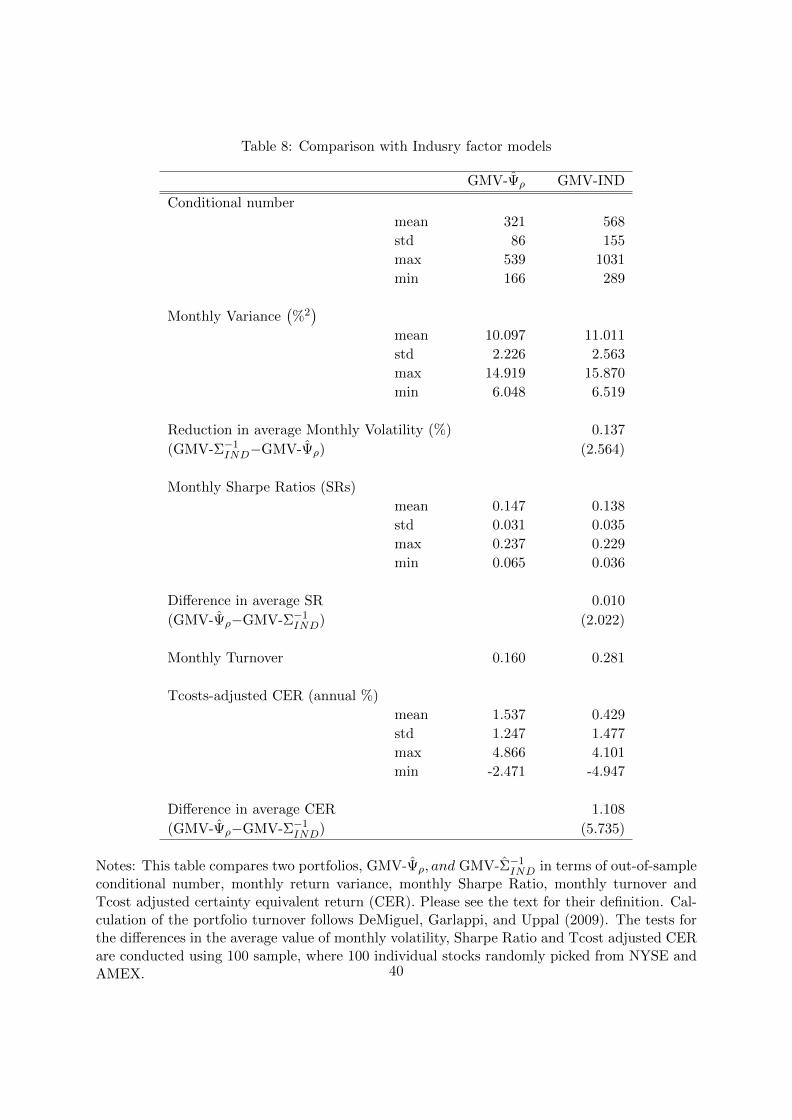
Table 8: Comparison with Indusry factor models

GMV-Ψρ GMV-IND

Conditional number

mean 321 568

std 86 155

max 539 1031

min 166 289

Monthly Variance(%2)

mean 10.097 11.011

std 2.226 2.563

max 14.919 15.870

min 6.048 6.519

Reduction in average Monthly Volatility (%) 0.137

(GMV-Σ−1IND−GMV-Ψρ) (2.564)

Monthly Sharpe Ratios (SRs)

mean 0.147 0.138

std 0.031 0.035

max 0.237 0.229

min 0.065 0.036

Difference in average SR 0.010

(GMV-Ψρ−GMV-Σ−1IND) (2.022)

Monthly Turnover 0.160 0.281

Tcosts-adjusted CER (annual %)

mean 1.537 0.429

std 1.247 1.477

max 4.866 4.101

min -2.471 -4.947

Difference in average CER 1.108

(GMV-Ψρ−GMV-Σ−1IND) (5.735)

Notes: This table compares two portfolios, GMV-Ψρ, and GMV-Σ−1IND in terms of out-of-sample

conditional number, monthly return variance, monthly Sharpe Ratio, monthly turnover andTcost adjusted certainty equivalent return (CER). Please see the text for their definition. Cal-culation of the portfolio turnover follows DeMiguel, Garlappi, and Uppal (2009). The tests forthe differences in the average value of monthly volatility, Sharpe Ratio and Tcost adjusted CERare conducted using 100 sample, where 100 individual stocks randomly picked from NYSE andAMEX. 40

Tab

le9:

Eff

ects

ofu

pd

atin

gρ

[1]

Mon

thly

Vari

ance

(%2)

[2]

Mon

thly

Sharp

eR

ati

o(S

R)

[3]

TC

ost

s-adju

sted

CE

R(a

nnual

%)

#Dataset

oldρ

new

ρw

ith

oldρ

wit

hnew

ρch

ange

wit

holdρ

wit

hnew

ρch

ange

wit

holdρ

wit

hnew

ρch

ange

1SZBM25

0.3

0.2

15.9

8915

.787

-0.2

020.

204

0.2

17

0.0

13

2.4

32

2.8

45

0.4

13

2SZBM100

1.7

0.8

15.6

97

15.3

47

-0.3

50

0.14

90.

140

-0.0

08

-0.7

77

-1.8

76

-1.0

98

4IN

D48

1.3

1.5

12.3

47

12.2

28

-0.1

19

-0.0

19

-0.0

16

0.0

03

-6.1

71

-5.9

37

0.2

34

6SZBM100+IN

D48

1.9

1.1

11.2

39

10.9

53

-0.2

86

0.11

30.

107

-0.0

06

-1.8

46

-2.6

37

-0.7

91

7IntM

kt0.

21.

020

.363

19.8

17

-0.5

45

0.16

60.

171

0.0

04

1.3

42

2.0

88

0.746

8IntValG

ro1.

11.

614

.961

15.1

38

0.17

60.

183

0.175

-0.0

08

0.4

33

0.6

69

0.236

9IntM

kt+IntValG

ro0.

81.

315

.150

14.8

54

-0.2

96

0.19

60.

191

-0.0

06

0.1

56

0.8

61

0.7

05

10MSCI

0.7

1.1

13.4

22

13.3

04

-0.1

18

0.05

60.

060

0.0

05

-2.7

53

-2.3

99

0.3

53

Not

es:

Th

ista

ble

exam

ines

the

effec

tof

up

dat

ingρs.

For

each

dat

aset

,w

esp

lit

the

ou

t-of-

sam

ple

test

ing

per

iod

into

two

even

hal

ves.

We

then

up

dat

eth

ees

tim

ati

onofρ

for

the

seco

nd

hal

fof

the

out-

of-s

amp

lete

stin

gp

erio

d,

then

reco

nst

ruct

the

GM

V-Ψ

ρ,

port

foli

o(‘

wit

hn

ewρ’)

,an

dco

mp

are

the

resu

lts

wit

hth

ose

pre

vio

us

resu

lts

wit

hou

tu

pd

ati

ngρ

(‘w

ith

oldρ’)

.T

he

com

pari

son

sare

new

resu

lts

min

us

old

resu

lts

inte

rms

of

[1]ou

t-of

-sam

ple

mon

thly

retu

rnva

rian

ce;

[2]m

onth

lyS

har

pe

Rat

io,an

d[3

]T

cost

-ad

just

edC

ER

.D

atase

t#

3an

d#

5ar

en

ot

inth

eco

mp

aris

onas

re-e

stim

ates

ofρ

do

not

gen

erat

ea

new

valu

e.

41