SAN DIEGO STATE UNIVERSITY

Department of Mathematics and Statistics

On Optimal Investment in the Long Run: Rank DependentExpected Utility as a “Bridge” between the

Maximum-Expected-Log and Maximum- Expected-UtilityCriteria

Vladimir Rotar

WORKING PAPER

December, 2002, the new version: December 24, 2003

Keywords and phrases: portfolio optimization, investment policy, the maximum expected utility, the maximum expected

logarithm.

Supported in part by the Russian Foundation of Basic Research, grant # 00-01-00194.

1

ABSTRACT

This paper concerns the well known paradox of inconsistency of the maximum-expected-utility (MEU)and the maximum-expected-log (MEL) criteria in investment dynamic models. The goal of the paperis to consider this phenomenon at the level of premises, and to suggest a generalized criterion, namelythe rank dependent expected utility (RDEU) approach which allows to “bridge the gap” between theMEU and MEL criteria. The preference order in the RDEU approach is preserved by the functional

U�F ����� ∞

0u�x � dΨ

�F�x �����

where F is a probability distribution, u is a utility function, and Ψ is a transforming or weightingfunction: the subject “transforms” the real distribution function F

�x � into another one, Ψ

�F�x �� ,

assigning different weights to different probabilities.

One of main goals of the paper is to establish conditions on the tail of Ψ, and on the utility functionu, under which the optimal investment in the long run corresponds to the MEL policy.

2

1 Introduction and an example.

1.1 Background and motivations

1.1.1 The MEU and MEL criteria.

This paper considers optimal investment in time, and concerns the long-known fact that the maximum-expected-utility (MEU) and the maximum-expected-log (MEL) criteria prove to be inconsistent evenfor large time horizons. This is, in a certain sense, a paradox since both criteria have reasonablejustifications based on assumptions which, though maybe are restrictive (as, say, the independenceaxiom), but are natural at least in the first approximation. Below we try to explain the inconsistencymentioned at the level of premises, and apply to this problem some relatively recent achievements ofthe modern utility theory. Specifically we make use of the rank dependent expected utility (RDEU)approach which, as will be seen, allows to “bridge the gap” between the MEU and MEL criteria, andin a sense to “reconcile” the results based on the two approaches.

The history of the question will be considered later in Section 1.1.4 after we state the problem.

Let the initial wealth of an investor W0 � 1, and the wealth after T periods of time

WT � WTπ � T

∏t � 1

�1�

Rt�π ����

where Rt�π � is the return in period t under an investment policy π. In the standard framework π is

a portfolio-vector, and Rt�π � � π � Rt , where Rt is the vector of the returns of assets in the market.

Below we do not need such a specification and may view π as a policy of a general nature.

Suppose that for each π the random returns � Ri�π ��� are independent and identically distributed

(i.i.d.), and at each period t the investor chooses the same policy not depending on the previous history(a “buy-and-hold” policy). In the asymptotic analysis the last assumption does not, in essence, restrictgenerality; we discuss this issue in more detail in Section 1.1.3. Nevertheless strategies π may dependon the horizon T .

Let m�π � : � E � ln � 1 � R1

�π ����� , and there exist a policy π � Argmax

πm�π � . If for a policy π and

some c � 0 it is true that m�π ��� m

�π � c, then (see references in Section 1.1.4)�

WT π � WTπ � � ∞ � as T � ∞, almost surely. (1.1.1)

The property (1.1.1) itself may serve as a desirable, though not necessary, requirement to anasymptotically optimal portfolio. In view of (1.1.1) it might seem that in the long run any “reasonable”policy π should be close in a sense to π. However, as is well known, it is not the case for the MEUcriterion

E � u � WTπ ��� ��� ∞

0u�x � dFTπ

�x � � (1.1.2)

where u�x � is the utility function of the investor, and FTπ is the distribution function of the random

variable (r.v.) WTπ. Say, if u�x ��� xα, then

E � u � WTπ ��� ��� E � � 1 � R1�π ��� α ��� T �

3

and the maximum is attained under a policy π�which maximizes E � � 1 � R1

�π ��� α � . Clearly, π

�is not

close to π in general, and cannot be close asymptotically since π�

does not depend on T at all. Formore complicated u, the analysis is more complex, but the conclusion is the same; see, e.g., Mertonand Samuelson (1974), Markowitz (1976), references therein and in Section 1.1.4. In Appendix 1 wegive a couple of simple but illustrative examples including that with a bounded utility function.

There has been a great deal of discussion on which criterion - MEU or MEL - is more preferableor realistic; see again Section 1.1.4. In this paper we are not concerned about which approach isbetter, but rather what makes them different, and the answer to this question is simple. Any integralcriterion of the type (1.1.2) takes into account possibilities of “very large” values occurring with “verysmall” probabilities, while the property (1.1.1) has to do only with probabilities, and in a certain senseeliminates events with negligible probabilities.

If one deals with fixed, not growing variables as, say, in a one-time fixed investment, the differencebetween the two criteria can be not significant. However, once we deal with growing variables (asWTπ in dynamics; for example, in a long period investment into a retirement fund), the differencementioned may be dramatic.

The question is whether it is possible, maintaining at least some features of the classical MEUcriterion, to make the decision process more flexible with respect to large deviations. One of possibleanswers is in making use of the Rank Dependent Expected Utility (RDEU) approach.

1.1.2 The RDEU criterion.

On a space of probability distributions F on�0 � ∞ � consider a preference ordering preserved by the

functionalU�F ����� ∞

0u�x � dΨ

�F�x ����� (1.1.3)

where u is a utility function, and the function Ψ is assumed to be non-decreasing, Ψ�0 � � 0 � Ψ �

1 � � 1 �The “transformation” function Ψ reflects the attitude of the subject to different probabilities: the

subject “transforms” the real distribution function F�x � into another one, Ψ

�F�x ��� , assigning different

weights to different probabilities.

For binary gambles such an approach was suggested by Kahneman and Tversky (1979) in theirProspect Theory, the full model was considered in Quiggin (1982), though some earlier Quigin’spapers contained some relevant ideas. For convenience of reading a brief survey of the RDEU theoryand some historical remarks are given in Appendix 2. A rather full history of the RDEU approach anda rich bibliography may be found in monographs Wakker (1989), Quiggin (1993), and Luce (2000).

A simple example is Ψ�p � � pβ. If β � 1, the subject perceives F as it is, and hence deals with the

“usual” expected utility (1.1.2). If β � 1, the investor overestimates the probability for the wealth to beless that a fixed value: the investor is “security-minded”. In the case β � 1, the investor underestimatesthe probability mentioned, being “potentially-minded” [see, e.g., Lopes (1987, 1990)].

A limiting example is a truncation: if for a fixed q � �0 � 1 �

�p ��� �

p if p � 1 � q �1 if p 1 � q �

then

U�F � � qu

�γq�F ��� � � γq � F �

0u�x � dF

�x ��� (1.1.4)

4

where γq�F � is the

�1 � q � -quantile of F . In this case the investor does not distinguish values greater

than γq�F � (viewed as too large) and occurring with a probability of q (viewed as too small). One may

consider it as the existence of a perception threshold. The functional (1.1.4) is not linear and shouldbe distinguished from the naive criterion when truncation is carried out at a fixed, perhaps, big valuenot depending on F .

If F is a distribution of a r.v. taking only two values, say, a and b � a with probabilities p and1 � p, respectively, then

U�F ��� u

�a � Ψ �

p � � u�b � �

1 � Ψ�p � � � (1.1.5)

and Ψ�p � “transforms” the probability p.

Let an investor having, say, the utility function u�x � � �

x, can choose from two future retirementplans: either the annual pension will be equal to X � $100 � 000, or to Y � $50 � 000 or $200 � 000with equal probabilities. (We do not consider here annuities in dynamics.) For the numbers abovethe expected utility criterion leads to a slight preference for the latter plan (E � u � X ����� 316 andE � u � Y � ��� 335), which for a large number of real people would hardly reflect their preferences. (Atleast the author would choose X .) On the other hand, under the criterion (1.1.5), as is easy to calculate,the investor would prefer X if Ψ

�1 � 2 � � 0 � 59 � 1 � 2, which means that such an investor would

slightly overestimate the probability of the unlucky event to get $50 � 000. So, one can expect Ψ�p � to

be concave for large p’s. Certainly, the above primitive example is given merely for illustration.

1.1.3 The goal of the paper.

In this paper we establish conditions on Ψ, under which the optimal policy converges to the MEL-policy as T � ∞. Roughly these conditions require the tail 1 � Ψ

�p � as p � 0, or/and Ψ

�p � as

p � 0, to vanish sufficiently fast. Though the conditions mentioned are non-necessary, as will beseen in Section 1.2, they are close in a certain sense to minimal. The asymptotic optimality of theMEL-policy is understood as follows.

Let � πT � denote a sequence of policies where the integer T � ∞. Suppose that for such a se-quence, and some c � 0

m�π ��� m

�πT � c

at least for large T , that is, πT is not optimal w.r.t. the MEL-criterion at least for large T . Then theconditions established in the next sections would imply that there exists T0 such that for all T � T0

U�FTπT � � U

�FT π ��� (1.1.6)

that is, πT is not optimal w.r.t. the RDEU-criterion (1.1.3) too.

If the space of policies under consideration is endowed by a metric � ��� - in the standard frameworkit may be Euclidean, and if the policy π is, in a certain sense, unique with respect to this metric(see Section 2.3 for detail), then for the policy πT maximizing U

�FTπ � , (1.1.6) would imply that

� πT � π � � 0, as T � ∞.

Probably it makes sense to say that such a result is not to be considered a justification of theRDEU criterion in portfolio optimization: it should be an object of a separate project. The goal ofthis paper is just to show that once we accept the RDEU framework, then the optimal policies may beclose, under certain conditions, to the MEL-policy. In my opinion, this fact itself is an argument infavor of the RDEU approach, but nevertheless the problem to what extent RDEU reflects real possibleinvestors’ preferences, is open.

5

The last but important remark concerns the fact that we deal here only with policies not dependingon the previous history. This is certainly a restriction but not as serious as it might look: under thei.i.d. assumption and some rather mild additional conditions optimal strategies are asymptotically, forlarge time horizons, close to stationary strategies of the type mentioned. However, the rigorous proofof this fact (especially when we apply the RDEU criterion) would take long calculations and make theframework and the result much less explicit. For this reason, to make the exposition clearer we startwith stationary buy-and-hold strategies from the very beginning: in the asymptotic analysis it doesnot, in essence, restrict generality.

In this connection it worthwhile to note that in practically all papers where the difference betweenthe MEL and MEU criteria has been discussed (for example, in basic papers by Merton and Samulel-son (1974), and Markowitz (1976)) the choice of policies under consideration was the same and, Ibelieve, for the same reason. The goal of this paper is in the introduction and analysis of a new cri-terion. So, it makes sense probably, at least in the first stage, to do this in the framework of the samemodel as has been considered before.

1.1.4 Historical remarks.

The MEL criterion itself was considered, for example, in Markowitz (1959), Latane (1959) andBreiman (1961). For properties of the MEL-portfolio as applied to bounded utilities see also Goldman(1974). A rather general model was investigated later in Algoet and Cover (1988), see also referencestherein.

It is worth noting that the maximization of the expected logarithm appears also in the analysisof stochastic analogues of the von Neumann-Gale model. In particular, the only natural stochasticanalogue of the von Neumann ray is the balanced path that maximizes the expected logarithm of thegrowth rate. See, e.g., Arnold, Evstigneev, Gundalach (1994), Evstigneev and Taksar (2001), andreferences therein.

Different aspects of the application of the MEU criterion to portfolio optimization were consideredin a great many of papers; see, e.g., Samuelson (1969), Hakansson (1971), Merton (1973), Breeden(1979); these papers also contain substantial reference lists.

The comparison of the two criteria, and a deep sophisticated discussion may be found in Samuel-son (1969, 1971), Goldman (1974), Merton and Samuelson (1974), Markowitz (1976), Ophir (1978,1979), Latane (1979), Samuelson (1979), and also in Markowitz’s remarks following Samuelson(1988).

One can find in the literature some remarks on the relevancy of large deviations to the inconsis-tency of the MEU and MEL criteria (see, e.g., Latane (1959), Ophir (1978, 1979); Samuelson (1979)),though all these remarks are implicit. To my knowledge, the only paper where the inconsistency ofthe MEL and MEU criteria has been explicitly connected with large deviations, is the unpublishedworking paper by Kim, Omberg and Russell (1993) [15].

In [15] the authors suggest to divide the whole space of elementary events in two groups: “non-extreme events” which correspond to “moderate” values of the wealth, and extreme events “to beremaining events farther out in the tails”. The authors suggest to consider the expected utility only overthe “non-extreme outcomes”, that is, to truncate integration in (1.1.2) by a “large” number dependingon T (the same for all F). Some examples in [15] show that it may lead to the MEL policy.

I do not know papers where the RDEU approach was applied to portfolio optimization, though in

6

general the idea of using RDEU in Economics is not new [see, e.g., Simonsen & Sergio (1991), Dowand Sergio (1992), Epstein and Tan Wang (1994), Mukerji & Tallon (1998), Tallon (1998), whichdoes not exhaust the whole possible references.

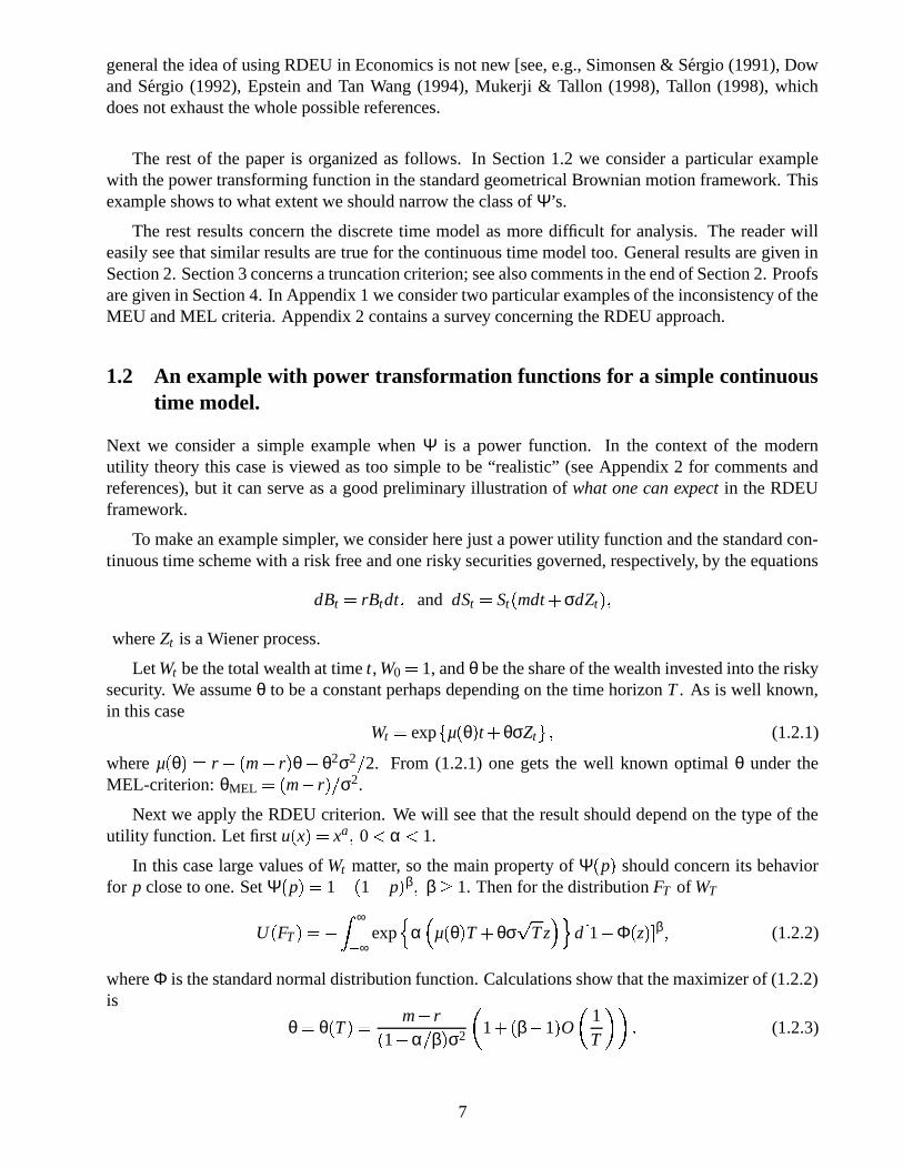
The rest of the paper is organized as follows. In Section 1.2 we consider a particular examplewith the power transforming function in the standard geometrical Brownian motion framework. Thisexample shows to what extent we should narrow the class of Ψ’s.

The rest results concern the discrete time model as more difficult for analysis. The reader willeasily see that similar results are true for the continuous time model too. General results are given inSection 2. Section 3 concerns a truncation criterion; see also comments in the end of Section 2. Proofsare given in Section 4. In Appendix 1 we consider two particular examples of the inconsistency of theMEU and MEL criteria. Appendix 2 contains a survey concerning the RDEU approach.

1.2 An example with power transformation functions for a simple continuoustime model.

Next we consider a simple example when Ψ is a power function. In the context of the modernutility theory this case is viewed as too simple to be “realistic” (see Appendix 2 for comments andreferences), but it can serve as a good preliminary illustration of what one can expect in the RDEUframework.

To make an example simpler, we consider here just a power utility function and the standard con-tinuous time scheme with a risk free and one risky securities governed, respectively, by the equations

dBt � rBtdt � and dSt � St�mdt

� σdZt ���where Zt is a Wiener process.

Let Wt be the total wealth at time t, W0 � 1, and θ be the share of the wealth invested into the riskysecurity. We assume θ to be a constant perhaps depending on the time horizon T . As is well known,in this case

Wt � exp � µ � θ � t � θσZt ��� (1.2.1)

where µ�θ � � r

� �m � r � θ � θ2σ2 � 2. From (1.2.1) one gets the well known optimal θ under the

MEL-criterion: θMEL � �m � r � � σ2.

Next we apply the RDEU criterion. We will see that the result should depend on the type of theutility function. Let first u

�x ��� xa � 0 � α � 1.

In this case large values of Wt matter, so the main property of Ψ�p � should concern its behavior

for p close to one. Set �p ��� 1 � �

1 � p � β � β 1. Then for the distribution FT of WT

U�FT ��� � � ∞� ∞

exp�

α � µ � θ � T � θσ�

T z ��� d�1 � Φ

�z � � β � (1.2.2)

where Φ is the standard normal distribution function. Calculations show that the maximizer of (1.2.2)is

θ � θ�T ��� m � r�

1 � α � β � σ2 � 1� �

β � 1 � O � 1T ��� � (1.2.3)

7

For β � 1 we naturally get the optimal policy in the Merton’s MEU model: θMEU � �m �

r � � � �1 � α � σ2 � (see, e.g., Duffie [6], Merton [28]). For β � 1 and large T the value θ shifts to θMEL,

andθ : � lim

T � ∞θ�T ��� m � r�

1 � α � β � σ2 �The greater the value of β, the closer θ is to θMEL, and farther from θMEU. In the limiting case β � ∞one has θ � θMEL. [If T � ∞, and β � ∞ simultaneously, the picture is more complicated, dependingon which characteristic grows faster. ]

Consider now u�x � � � x

� α � α � 0. Unlike in the previous case, here small values of Wt matter.Hence now the asymptotics of Ψ

�p � for p � 0 is important. Set Ψ

�p � � pβ � β 1. It is not difficult

to calculate that in this case the maximizer of U�FT � is

θ�T � � m � r�

1� α � β � σ2 � 1

� �β � 1 � O � 1

T � � � (1.2.4)

to which similar comments apply.

Thus, though the power transforming function causes a shift towards the MEL policy, for theoptimal policy to converge to the MEL strategy, as T � ∞, the tail of Ψ

�p � should vanish faster than

a power function. It is lucky that this is the case that - for other reasons - attracted the attention of anumber of researchers last years. We use one of these results in the next section.

2 A discrete time model: general results.

2.1 Conditions on Ψ.

Note first that the criterion (1.1.3) is often specified in the literature in terms of the function w�p � �

1 � Ψ�1 � p � which is referred to as a weighting function. If u

�0 � � 0 (which does not restricts

generality if u�x � is bounded from below),

U�F � � � ∞

0w�1 � F

�x ��� du

�x � �

In some calculations the last representation proves to be more convenient.

We make here use of the relatively recent but already well known result by Prelec (1998), whoestablished axioms under which the weighting function admits the explicit representation

w�p ��� wβη

�p ��� exp � � � � β ln

�p � � η � � (2.1.1)

where β � η are positive parameters. The corresponding transformation function Ψβη�p � � 1 � wβη

�1 �

p � .Prelec’s axioms and some properties of (2.1.1) are discussed in Appendix 2. Now we just note

that if η � 1, then (2.1.1) directly leads to the power function pβ, while for η � 1 the function wβηis S-shaped, and wβη

�p � � 0 as p � 0 (and hence Ψβη

�p � � 1 as p � 1) faster than any power

function. In this case the subject is “strongly security-minded”, and in a rather small degree takes intoaccount possibilities of “lucky” large deviations.

8

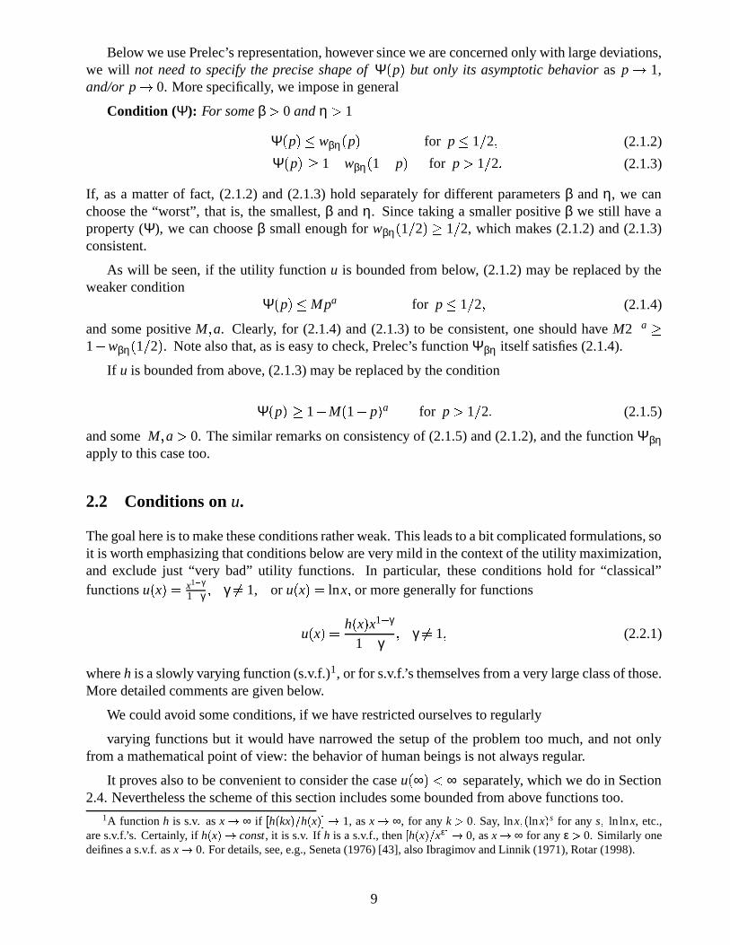
Below we use Prelec’s representation, however since we are concerned only with large deviations,we will not need to specify the precise shape of Ψ

�p � but only its asymptotic behavior as p � 1,

and/or p � 0. More specifically, we impose in general

Condition (Ψ): For some β � 0 and η � 1

Ψ�p � � wβη

�p � for p

�1 � 2 � (2.1.2)

Ψ�p � 1 � wβη

�1 � p � for p � 1 � 2 � (2.1.3)

If, as a matter of fact, (2.1.2) and (2.1.3) hold separately for different parameters β and η, we canchoose the “worst”, that is, the smallest, β and η. Since taking a smaller positive β we still have aproperty (Ψ), we can choose β small enough for wβη

�1 � 2 � 1 � 2, which makes (2.1.2) and (2.1.3)

consistent.

As will be seen, if the utility function u is bounded from below, (2.1.2) may be replaced by theweaker condition

Ψ�p � � Mpa for p

�1 � 2 � (2.1.4)

and some positive M � a. Clearly, for (2.1.4) and (2.1.3) to be consistent, one should have M2� a

1 � wβη�1 � 2 � . Note also that, as is easy to check, Prelec’s function Ψβη itself satisfies (2.1.4).

If u is bounded from above, (2.1.3) may be replaced by the condition

Ψ�p � 1 � M

�1 � p � a for p � 1 � 2 � (2.1.5)

and some M � a � 0. The similar remarks on consistency of (2.1.5) and (2.1.2), and the function Ψβηapply to this case too.

2.2 Conditions on u.

The goal here is to make these conditions rather weak. This leads to a bit complicated formulations, soit is worth emphasizing that conditions below are very mild in the context of the utility maximization,and exclude just “very bad” utility functions. In particular, these conditions hold for “classical”functions u

�x ��� x1 � γ

1 � γ � γ �� 1, or u�x � � lnx � or more generally for functions

u�x ��� h

�x � x1 � γ

1 � γ� γ �� 1 � (2.2.1)

where h is a slowly varying function (s.v.f.)1, or for s.v.f.’s themselves from a very large class of those.More detailed comments are given below.

We could avoid some conditions, if we have restricted ourselves to regularly

varying functions but it would have narrowed the setup of the problem too much, and not onlyfrom a mathematical point of view: the behavior of human beings is not always regular.

It proves also to be convenient to consider the case u�∞ � � ∞ separately, which we do in Section

2.4. Nevertheless the scheme of this section includes some bounded from above functions too.1A function h is s.v. as x � ∞ if � h � kx ��� h � x ��� 1, as x � ∞, for any k � 0 Say, lnx ��� lnx � s for any s � ln lnx, etc.,

are s.v.f.’s. Certainly, if h � x ��� const, it is s.v. If h is a s.v.f., then � h � x ��� xε �� 0, as x � ∞ for any ε � 0. Similarly onedeifines a s.v.f. as x � 0. For details, see, e.g., Seneta (1976) [43], also Ibragimov and Linnik (1971), Rotar (1998).

9

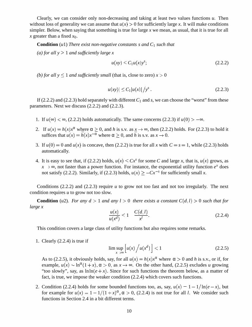
Clearly, we can consider only non-decreasing and taking at least two values functions u. Thenwithout loss of generality we can assume that u

�x � � 0 for sufficiently large x. It will make conditions

simpler. Below, when saying that something is true for large x we mean, as usual, that it is true for allx greater than a fixed x0.

Condition (u1) There exist non-negative constants s and C1 such that

(a) for all y 1 and sufficiently large x

u�xy � � C1u

�x � ys; (2.2.2)

(b) for all y�

1 and sufficiently small (that is, close to zero) x � 0

�u�xy � � � C1

�u�x � � �

ys � (2.2.3)

If (2.2.2) and (2.2.3) hold separately with different C1 and s, we can choose the “worst” from theseparameters. Next we discuss (2.2.2) and (2.2.3).

1. If u�∞ � � ∞, (2.2.2) holds automatically. The same concerns (2.2.3) if u

�0 � � � ∞.

2. If u�x ��� h

�x � xα where α 0, and h is s.v. as x � ∞, then (2.2.2) holds. For (2.2.3) to hold it

suffices that u�x ��� h

�x � x � α where α 0, and h is s.v. as x � 0.

3. If u�0 � � 0 and u

�x � is concave, then (2.2.2) is true for all x with C � s � 1, while (2.2.3) holds

automatically.

4. It is easy to see that, if (2.2.2) holds, u�x � �

Cxs for some C and large x, that is, u�x � grows, as

x � ∞, not faster than a power function. For instance, the exponential utility function ex doesnot satisfy (2.2.2). Similarly, if (2.2.3) holds, u

�x � � Cx

� s for sufficiently small x.

Conditions (2.2.2) and (2.2.3) require u to grow not too fast and not too irregularly. The nextcondition requires u to grow not too slow.

Condition (u2). For any d � 1 and any l � 0 there exists a constant C�d � l � � 0 such that for

large xu�x �

u�xd � �

1 � C�d � l �xl � (2.2.4)

This condition covers a large class of utility functions but also requires some remarks.

1. Clearly (2.2.4) is true if

lim supx � ∞

�u�x ��� u

�xd ��� � 1 (2.2.5)

As to (2.2.5), it obviously holds, say, for all u�x � � h

�x � xα where α � 0 and h is s.v., or if, for

example, u�x ��� lnα � 1 � x ��� α � 0 � as x � ∞. On the other hand, (2.2.5) excludes u growing

“too slowly”, say, as lnln�e�

x � � Since for such functions the theorem below, as a matter offact, is true, we impose the weaker condition (2.2.4) which covers such functions.

2. Condition (2.2.4) holds for some bounded functions too, as, say, u�x � � 1 � 1 � ln

�e�

x � , butfor example for u

�x � � 1 � 1 � � 1 � x � α � α � 0, (2.2.4) is not true for all l. We consider such

functions in Section 2.4 in a bit different terms.

10

3. Functions that grow as power ones at least for sequences of x’s, but do not satisfy (2.2.4),certainly exist but look exotic. Let, say, u

�xk ��� �

xk for xk � exp � 4k � , k � 1 � 2 � � � � , and u�x � is

constant on�xk � xk

�1 � . Then

�u�xk � �

u�x2

k ��� � 1 for all k, that is, (2.2.4) is not true for d � 2.

4. It is not true however that (2.2.4) holds for any s.v.f. tending to infinity, but examples are ratherexotic and we skip them here.

2.3 The main theorem.

First we need some conditions on r.v.’s Rt�π � .

Conditions (R).

(1) There exists a policy π maximizing m�π � , and m : � m

�π � � 0.

(2) Supposesup

πσ�π � � ∞ � (2.3.1)

where σ2 � π � : � Var � ln � 1 � R1�π ����� .

(3) For a positive c0, and all π�ln�1�

R1�π � � � m

�π � � � c0σ

�π � � (2.3.2)

that is, the normalized r.v.�ln�1�

R1�π �� � m

�π � � � σ � π � is bounded uniformly in π.

The third requirement is imposed to avoid complicated conditions on the tails of the distributionsof Rt

�π � . It means, in particular, that the r.v. ln

�1�

R1�π � � is bounded, and it excludes policies π

for which the variance σ2 � π � is “very small” while the r.v. ln�1�

R1�π �� itself may take “not small”

values with “very small” probabilities.

Certainly it excludes, say, log-normally distributed r.v.’s , but for the discrete time model and froma “realistic” point of view such a restriction is not too strong.

Next we consider the first result. When comparing the policy π with a policy π, we presupposethat π � πT , that is, perhaps depends on T . This is the case, for example, if we consider a policymaximizing U

�FTπ � . When considering a sequence of policies � πT � we assume that the integer

parameter T � ∞ but perhaps takes not all sequential natural values, that is, � πT � � � πT1 � πT2 � � � � �where � Tk � is an increasing sequence of integers, and Tk � ∞, as k � ∞.

Theorem 1 Assume that conditions (Ψ), (u1), (u2) and (R) hold. Suppose that for a sequence � πT �and a fixed c � 0 it is true that m

�π � � m

�πT � c at least for large T . Then there exists T0 perhaps

depending on the sequence � πT � and such that for all T � T0

U�FTπT � � U

�FT π � � (2.3.3)

If u�0 � � � ∞, condition (2.2.3) in (u1) holds automatically, and instead of (2.1.2) in (Ψ) it suffices

to assume (2.1.4) to be true for some positive M and a.

11

Let now the space of all possible policies be endowed by a metric � � � , and π is unique w.r.t. thismetric in the following usual sense.

Condition (π) : For each δ � 0 there exists a positive ε depending only on δ and such that, if� π � π � δ, then m

�π � � m

�π � ε.

Clearly, Theorem 1 implies

Corollary 2 Suppose that all conditions of Theorem 1 plus condition (π) hold, and for each T thereexists a policy πT maximizing U

�FTπ � � Then � πT � π � � 0 � as T � ∞.

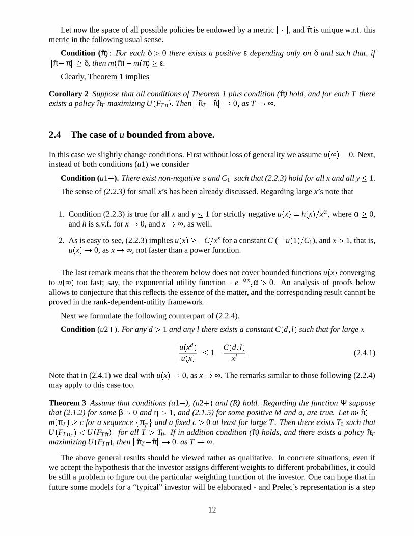
2.4 The case of u bounded from above.

In this case we slightly change conditions. First without loss of generality we assume u�∞ � � 0. Next,

instead of both conditions (u1) we consider

Condition (u1�

). There exist non-negative s and C1 such that (2.2.3) hold for all x and all y�

1.

The sense of (2.2.3) for small x’s has been already discussed. Regarding large x’s note that

1. Condition (2.2.3) is true for all x and y�

1 for strictly negative u�x � � h

�x � � xα, where α 0,

and h is s.v.f. for x � 0, and x � ∞, as well.

2. As is easy to see, (2.2.3) implies u�x � � C � xs for a constant C ( � u

�1 � � C1), and x � 1, that is,

u�x � � 0, as x � ∞, not faster than a power function.

The last remark means that the theorem below does not cover bounded functions u�x � converging

to u�∞ � too fast; say, the exponential utility function � e

� αx � α � 0. An analysis of proofs belowallows to conjecture that this reflects the essence of the matter, and the corresponding result cannot beproved in the rank-dependent-utility framework.

Next we formulate the following counterpart of (2.2.4).

Condition (u2�

). For any d � 1 and any l there exists a constant C�d � l � such that for large x

����

u�xd �

u�x �

����

�1 � C

�d � l �xl � (2.4.1)

Note that in (2.4.1) we deal with u�x � � 0, as x � ∞. The remarks similar to those following (2.2.4)

may apply to this case too.

Theorem 3 Assume that conditions (u1�

), (u2� � and (R) hold. Regarding the function Ψ suppose

that (2.1.2) for some β � 0 and η � 1, and (2.1.5) for some positive M and a, are true. Let m�π � �

m�πT � c for a sequence � πT � and a fixed c � 0 at least for large T . Then there exists T0 such that

U�FTπT � � U

�FT π � for all T � T0. If in addition condition (π) holds, and there exists a policy πT

maximizing U�FTπ � , then � πT � π �� 0 � as T � ∞.

The above general results should be viewed rather as qualitative. In concrete situations, even ifwe accept the hypothesis that the investor assigns different weights to different probabilities, it couldbe still a problem to figure out the particular weighting function of the investor. One can hope that infuture some models for a “typical” investor will be elaborated - and Prelec’s representation is a step

12

in this direction, but for now this topic is not so developed. In the light of this, the simple but explicittruncation criterion could occur to be useful. In the next section we consider it in detail. It will allowto remove or essentially weaken some conditions, and to consider a quantitative estimate for the timeT0.

3 On the truncation criterion

To include into consideration a larger class of utility function we consider truncation from both sides.More specifically, we fix q � �

0 � 1 � , and consider the criterion

U�F ��� q

�u�γq� � F ��� � u

�γq � � F ��� � �

γq� � F ��

γq � � F �u�x � dF

�x � � (3.1)

where γq � � F � and γq� � F � are q- and

�1 � q � - quantiles of F , respectively. As was noted in Section

1.1.2 this is a limiting case of the rank dependent utility: the investor does not distinguish “too large”values occurring with a small probability of q, as well as “too small values” occurring with the sameprobability. Truncation in the areas of large and small values should be interpreted differently. If aninvestor does not distinguish too large values of gains, she exhibits a threshold of perception in thezone of “lucky” events, demonstrating a cautious behavior. On the other hand, if the investor does notdistinguish too small values of the wealth, that is, too large values of losses, she has a threshold ofperception in the area of ruin. It reflects the well known phenomenon when people exhibit differenttypes of behavior depending on whether they deal with gains or losses (see, e.g., Luce (2000)).

By the sense of the problem, q is small, so we can assume q�

1 � 4.

In view of (2.3.1)

WTπ � exp�

m�π � T � σ

�π � � T � ξTπ � � (3.2)

where

ξTπ � lnWTπ � m�π � T

σ�π � � T

� ∑Tt � 1

�ln�1�

Rt�π � � � m

�π � �

σ�π � � T

is asymptotically normal for each π such that σ�π � �� 0. If σ

�π � � 0, we can define ξTπ as a standard

normal r.v.; it will not cause a misunderstanding below.

For each pair of distributions F and G, set � F � G � ∞ � supx�F�x � � G

�x � � . Let, as before, FTπ

�x � �

P�WTπ

�x � , F

�

Tπ�x ��� P

�ξT

�x � and ∆T

�π � � � F �

Tπ � Φ � ∞. Clearly, ∆T�π � � 0, as T � ∞, for each

π �Condition (UNA: Uniform Normal Approximation):

supπ

∆T�π � � 0 � as T � ∞. (3.3)

It is a rather weak condition. For example, since by the Berry-Esseen theorem (see, e.g., [9]) ifσ�π � �� 0, then

∆T�π � � β

�π �

σ3�π � � T

� (3.4)

13

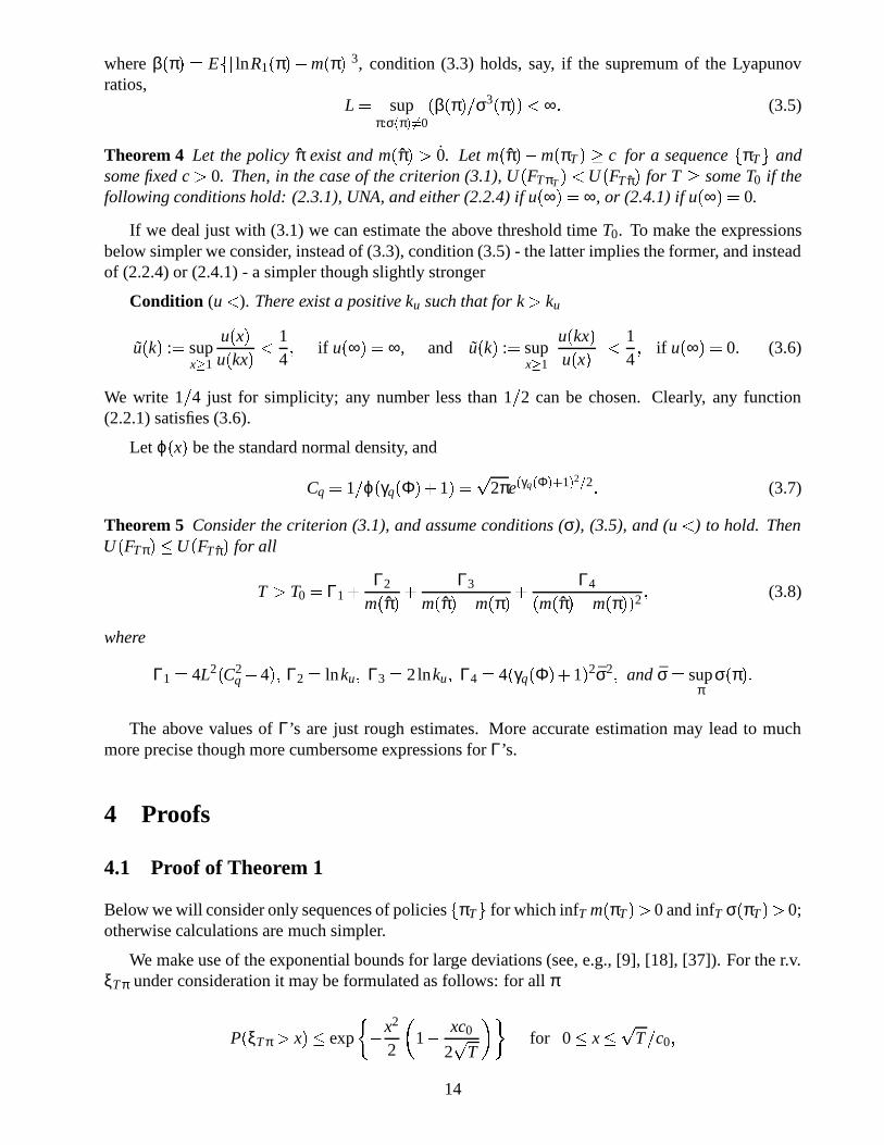
where β�π � � E � � lnR1

�π � � m

�π � � 3, condition (3.3) holds, say, if the supremum of the Lyapunov

ratios,L � sup

π:σ � π � �� 0

�β�π � � σ3 � π ��� � ∞ � (3.5)

Theorem 4 Let the policy π exist and m�π � � 0. Let m

�π � � m

�πT � c for a sequence � πT � and

some fixed c � 0. Then, in the case of the criterion (3.1), U�FTπT � � U

�FT π � for T some T0 if the

following conditions hold: (2.3.1), UNA, and either (2.2.4) if u�∞ � � ∞, or (2.4.1) if u

�∞ � � 0.

If we deal just with (3.1) we can estimate the above threshold time T0. To make the expressionsbelow simpler we consider, instead of (3.3), condition (3.5) - the latter implies the former, and insteadof (2.2.4) or (2.4.1) - a simpler though slightly stronger

Condition (u � ). There exist a positive ku such that for k � ku

u�k � : � sup

x � 1

u�x �

u�kx � � 1

4� if u

�∞ � � ∞, and u

�k � : � sup

x � 1

����

u�kx �

u�x �

����

� 14� if u

�∞ ��� 0. (3.6)

We write 1 � 4 just for simplicity; any number less than 1 � 2 can be chosen. Clearly, any function(2.2.1) satisfies (3.6).

Let ϕ�x � be the standard normal density, and

Cq � 1 � ϕ � γq�Φ � � 1 � � �

2πe � γq � Φ � � 1 � 2 � 2 � (3.7)

Theorem 5 Consider the criterion (3.1), and assume conditions (σ), (3.5), and (u � ) to hold. ThenU�FTπ � �

U�FT π � for all

T � T0 � Γ1� Γ2

m�π � � Γ3

m�π � � m

�π � � Γ4�

m�π � � m

�π ��� 2 � (3.8)

where

Γ1 � 4L2 � C2q�

4 ��� Γ2 � lnku � Γ3 � 2lnku � Γ4 � 4�γq�Φ � � 1 � 2σ2 � and σ � sup

πσ�π � �

The above values of Γ’s are just rough estimates. More accurate estimation may lead to muchmore precise though more cumbersome expressions for Γ’s.

4 Proofs

4.1 Proof of Theorem 1

Below we will consider only sequences of policies � πT � for which infT m�πT � � 0 and infT σ

�πT � � 0;

otherwise calculations are much simpler.

We make use of the exponential bounds for large deviations (see, e.g., [9], [18], [37]). For the r.v.ξTπ under consideration it may be formulated as follows: for all π

P�ξTπ � x � � exp

�� x2

2 � 1 � xc0

2�

T � �for 0

�x� �

T � c0 �14

P�ξTπ � x � � exp

�� x

�T

4c0 � for x �T � c0 �

where c0 is the constant from (2.3.2). The same bounds are true for P�ξT � � x ��� x � 0 �

We simplify this as

P�ξTπ � x � �

gT�x ��� P

�ξTπ � � x � � gT

�x � � (4.1.1)

where x is arbitrary, and

gT�x � � ���� 1 for x � 0 �

exp � � x2 � 4 � for 0�

x� �

T � c0 �exp � � x

�T � 4c0 � for x �

T � c0 �(4.1.2)

Set, as before, FTπ�x � � P

�WTπ

�x � , and F

�

Tπ�x � � P

�ξTπ

�x � . If it cannot cause a misunder-

standing, we omit sometimes the index T in πT , and the index π in ξTπ, FTπ and F�

Tπ, and write m andσ instead of m

�π � and σ

�π � .

As usual, saying below that something, for example, an inequality, is true for large T we meanthat it is true for all T greater or equal than some fixed T1.Once it has been said, for the rest of theproof we consider only T T1. It means, in particular, that if, say, another inequality is true for T some T2, than we consider T max � T1 � T2 � . We will not repeat it each time. The numbers T1 � T2, etc.,mentioned depend perhaps on parameters of the problem: c0 � C1 � M � a, etc.

Let c be a continuity point of Ψ�F

�

T

�x ��� . Then,

U�FT ��� � ∞

0u�x � dΨ

�FT

�x ����� � ∞� ∞

u�emT eσ � Ty � dΨ

�F

�

T�y ���

� � c � 0� ∞u�emT eσ � Ty � dΨ

�F

�

Tπ�y ��� � � ∞

cu�emT eσ � Ty � d �

1 � Ψ�F

�

T�y �� �

� � c� ∞u�emT eσ � Ty � dΨ

�F

�

Tπ�y ��� � � ∞

cu�emT eσ � Ty � d �

1 � Ψ�F

�

T�y ��� �

� u�emT eσ � Tc � � � ∞

c

�1 � Ψ

�F

�

T�y ��� � du

�emT eσ � Ty � � � c� ∞

Ψ�F

�

T�y ��� du

�emT eσ � Ty � � (4.1.3)

Hence, by (4.1.1) and since u is non-decreasing, for c 0,

U�FT � �

u�emT eσ � Tc � � � ∞

c

�1 � Ψ

�1 � gT

�y ��� � du

�emT eσ � Ty � � (4.1.4)

Let Ψ�p � be any non-decreasing and continuous at zero function such that Ψ

�0 � � 0 � Ψ �

1 � � 1, andΨ�p � � Ψ

�p � for all p. Then (4.1.4) implies that

U�FT � �

u�emT eσ � Tc � � � ∞

c

�1 � Ψ

�1 � gT

�y ��� � du

�emT eσ � Ty �

� u�emT eσ � Tc � Ψ �

1 � gT�c ��� � � ∞

cu�emT eσ � Ty � dΨ

�1 � gT

�y ��� �

Since c can be chosen arbitrary close to zero and Ψ�p � is continuous at zero, eventually

U�FT � � � ∞

0u�emT eσ � Ty � dΨ

�1 � gT

�y ��� � (4.1.5)

15

Recall that in the case of Theorem 1 we assume that u�x � � 0 for sufficiently large x. Consequently,

since we consider only the case infT m�πT � � 0, for sufficiently large T all values of u

�emT eσ � Ty � in

the r.-h.s. of (4.1.5) are positive for all y. Set

k1 � k1�T � � 2β � 1 � 2T 1 � 2η � (4.1.6)

Since η � 1 � there exists T1 � T1�β � η � such that for T T1 one has k1

�T � � �

T � c0. So, for T max � T1 � � β ln2 � η �

gT�k1 ��� exp � � k2

1 � 4 � � exp � � T 1 � η � β � �1 � 2 � (4.1.7)

Then we can use (2.1.3) and set Ψ�p � � 1 � wβη

�1 � p � for p 1 � 2, and Ψ

�p � � min � Ψ �

p ��� 1 �wβη

�1 � p ��� for p � 1 � 2. The Ψ so chosen is continuous at zero. By (4.1.5)

U�FT � � � ∞

0u�emT eσ � Ty � dΨ

�1 � gT

�y ����� k1�

0

� ∞�k1

� J1�

J2 � (4.1.8)

For J1 it suffices to write

J1�

u�exp � mT

�k1σ

�T � ��� u

�exp � mT

�2σβ � 1 � 2T � 1 � η � � 2η � � � (4.1.9)

where the r.-h.s. is positive for large T .

For large T we have also 1 � gT�k1�T ��� � 1 � 2, and hence Ψ

�1 � gT

�y ��� � 1 � wβη

�gT

�y �� for

y k1�T � . Next we use (2.2.2) which is true for x � some x1. Since exp � mT

�k1�T � σ � T � � x1 for

large T , we can use (2.2.2) when estimating J2. Consequently, for sufficiently large T

J2 � ∞�k1

u�emT eσ � Ty � d � � wβη

�gT

�y ��� � �

C1u�emT � I � (4.1.10)

where

I � I�T ��� ∞�

k1 � T �exp � sσ

�T y � d � � wβη

�gT

�y ��� � � (4.1.11)

As was told already, k1�T � � �

T � c0 for large T , and hence we can write

I � ∞�k1

� � T � c0�k1

� ∞�� T � c0

� I1�

I2 �

Furthermore,

I1 � I1�T � � � T � c0�

k1 � T �exp � sσ

�T y � d � � wβη

�gT

�y ��� �

� � T � c0�k1 � T �

exp�

sσ�

T y � d�� exp

�� �

βy2 � 4 � η � � ��

β � T � 2c0��

βk1 � T � � 2

exp�

2β � 1 � 2sσ�

T y � d� � exp � � y2η � �

� ∞��

βk1 � T � � 2

exp�

2β � 1 � 2sσ�

T y � d� � exp � � y2η � � � (4.1.12)

16

Thus, we need an estimate for integrals of the type

∞�R

xl exp � tx � x2η � dx� ∞�

R

xl exp � tx � x2R2η � 2 � dx

� 1

R � η � 1 � � l � 1 �∞�

Rη

yl exp � � t � Rη � 1 � y � y2 � dx� C

�l �

R � η � 1 � � l � 1 �∞�

Rη

exp � � t � Rη � 1 � y � y2 � 2 � dx

� C�l �

R � η � 1 � � l � 1 � exp

�12� t � Rη � 1 � 2

� ∞�Rη

exp � � � y � �t � Rη � 1 �� 2 � 2 � dx

� C�l �

R � η � 1 � � l � 1 � exp

�12� t � Rη � 1 � 2

� �1 � Φ

�Rη � �

t � Rη � 1 ��� � �where C

� � � as usual, denotes a constant depending only on the argument in� � � , and which may be

different in different formulas. Applying the last inequality to (4.1.12), we have

I1�T � � C

�η � � 2β � 1 � 2 � � η � 1 � 2η

k�η � 1 � 2η

1

�T � exp

�12� � 2 � � β � ηsσ

�T � kη � 1

1 � 2�

� �1 � Φ � � � βk1 � 2 � η � �

2 ��

β � ηsσ�

T � kη � 11 � �

� C�η �

T�η � 1 � exp

�2β � 1s2σ2T 1 � η � �

1 � Φ � � T � 2β � 1 � 2sσT 1 � 2η � � � (4.1.13)

It suffices now to use that

� 1x� 1

x3 � ϕ�x � � 1 � Φ

�x � � Φ

� � x � � 1x

ϕ�x ��� for x � 0 � (4.1.14)

where ϕ�x � � Φ

� �x � (see, e.g., [9], [18], [37]). Set σ � supπ σ

�π � � ∞ in view of (2.3.1). It is straight-

forward to derive from (4.1.13) and (4.1.14) that, if η � 1, then there exists T2 � T2�σ � C1 � β � η � s � such

that for T T2

I1�T � � e

� T � 4 � (4.1.15)

Furthermore,

I2�T � � ∞�� T � c0

exp � sσ�

T y � d � � wβη�exp � � y

�T � 4c0 � � �

� ∞�� T � c0

exp�

sσ�

T y � d

�� exp

���βy�

T4c0 � η ���

� ∞�βT � 4c2

0

exp � � 4c0β � 1sσ � z � d� � exp � � zη � � � (4.1.16)

We see that there exists T3 � T3�c0 � C1 � β � η � s � such that for all T T3

I2�

e� T � (4.1.17)

17

From (4.1.15) and (4.1.17) it follows that for large T

I�T � � e

� T � 4 � e� T �

2e� T � 4 � (4.1.18)

and henceJ2

�C1u

�emT � � e � T � 4 � e

� T � � u�emT � e � T � 5 (4.1.19)

for sufficiently large T .

Collecting (4.1.8), (4.1.9), and (4.1.19), we obtain that for sufficiently large T

U�FT � �

u�exp � mT

�2σβ � 1 � 2T � 1 � η � � 2η � � � u

�emT � e � T � 5

�u�exp � mT

�2σβ � 1 � 2T � 1 � η � � 2η � � �

1�

e� T � 5 � � (4.1.20)

where the r.-h.s. is positive.

We turn to lower bounds for U�FT � . Let c be a continuity point of Ψ

�F

�

T

�y ��� , and c

�0. Then, by

(4.1.3),

U�FT � u

�emT eσ � Tc � � � c� ∞

Ψ�F

�

T�y ��� du

�emT eσ � Ty � u

�emT eσ � Tc � � � c� ∞

Ψ�gT

� � y ��� du�emT eσ � Ty � �

(4.1.21)

Let now Ψ�p � be any non-decreasing and continuous at p � 1 function such that Ψ

�0 � � 0 � Ψ �

1 � �1, and Ψ

�p � Ψ

�p � for all p. Then it follows from (4.1.21) that

U�FT � u

�emT eσ � Tc � � � c� ∞

Ψ�gT

� � y ��� du�emT eσ � Ty �

� u�emT eσ � Tc � � 1 � Ψ

�gT

� � c ����� � � c� ∞u�emT eσ � Ty � dΨ

�gT

� � y ��� u

�emT eσ � Tc � � 1 � Ψ

�gT

� � c ����� � � ∞�c

� u�emT e

� σ � Ty � d � � Ψ�gT

�y ��� � �

Since c can be chosen arbitrary close to zero and Ψ�p � is continuous at one,

U�FT � � ∞

0u�emT e

� σ � Ty � d � � Ψ�gT

�y ��� � (4.1.22)

Let now x0 be the number such that u�x � �

0 for x � x0, and u�x � � 0 for x � x0. By con-

dition (u1) there exists x2�

x0 such that (2.2.3) holds for x�

x2. Let y0 � y0�T � � m

�T σ � 1 ��

lnx0 � � σ � T � � 1 � y2 � y2�T � � m

�T σ � 1 � �

lnx2 � � σ � T � � 1. Clearly, k1�T � � y0

�T � �

y2�T � for

large T .

Set Ψ�p � � wβη

�p � for p

�1 � 2, and Ψ

�p � � max � wβη

�p � � Ψ �

p ��� otherwise. Note that �p � is

continuous at p � 1. Furthermore

U�FT � � ∞

0u�emT e

� σ � Ty � d � � Ψ�gT

�y ��� � � � k1

0

� � y0

k1

� � y2

y0

� � ∞

y2

� J3�

J4�

J5�

J6 � (4.1.23)

Considering T large enough for gT�k1�T ��� � 1 � 2, we get that

18

J3 u�exp � mT � k1

�T � σ � T � � �

1 � Ψ�gT

�k1�T ����� � � u

�exp � mT � k2

�T � σ � T � � �

1 � wβη�gT

�k1�T ����� �

� u�exp � mT � 2σβ � 1 � 2T � 1 � η � � 2η � � �

1 � e� T � � (4.1.24)

where the r.-h.s. is positive for large T .

It suffices to write J4 0. The next integral

J5 � � u � x2 � � Ψ �gT

�y0 ��� � � u � x2 � �wβη

�gT

�y0 ��� � � u � x2 � �wβη

�gT

�k1 ��� � � � u � x2 � � e � T � (4.1.25)

Furthermore, for y y2 we can use (2.2.3) in the following way

J6 � � ∞

y2

u�emT e

� σ � Ty � d � � wβη�gT

�y ��� � � � ∞

y2

u�x2 exp � � σ

�T�y � y2 ��� � d � � wβη

�gT

�y ��� �

� ∞

y2

u�x2 exp � � σ

�T y � � d � � wβη

�gT

�y ��� � C1u

�x2 � � ∞

y2

exp � sσ�

T y � � d � � wβη�gT

�y ��� �

� C1�u�x2 � � � ∞

k1

exp � sσ�

T y � � d � � wβη�gT

�y ��� � � 2C1

�u�x2 � � e � T � 4 (4.1.26)

for large T in view of (4.1.18).

Since there exists a constant C2 � 0, perhaps depending on parameters of the problem, such thatu�mT � 2σβ � 1 � 2T � 1 � η � � 2η � C2 for large T , (4.1.23), (4.1.24), (4.1.25), and (4.1.26) imply for large

T that

U�FT � u

�exp � mT � 2σβ � 1 � 2T � 1 � η � � 2η � � �

1 � e� T � C

� 12

�u�x2 � � � e � T � 2C1e

� T � 4 � � u

�exp � mT � 2σβ � 1 � 2T � 1 � η � � 2η � � �

1 � e� T � 5 � � (4.1.27)

where the r.-h.s. is positive.

Turning to the last step of the proof, we fix a policy π and write FT , m � σ for FTπ � m �π ��� σ � π � ,

respectively. Symbols FT � m � σ will correspond to the policy π.

Let ∂m : � m � m c � 0. Combining (4.1.20) and (4.1.27), taking into account that η � 1, andmaking use of (2.2.4), we have for large T

U�FT �

U�FT � � u

�exp � mT

�2σβ � 1 � 2T � 1 � η � � 2η � � �

1�

e� T � 5 �

u�exp � mT � 2σβ � 1 � 2T � 1 � η � � 2η � � �

1 � e � T � 5 �� u

�exp � � m � ∂m � 4 � T ��� � �

1�

e� T � 5 �

u�exp � � m � ∂m � 4 � T ��� � �

1 � e � T � 5 �� �

1 � C�l � d � exp � � l

�m� ∂m � 4 � T � ��� � 1 � 3e

� T � 5 � � (4.1.28)

where d � m � ∂m � 4m� ∂m � 4 4m � c

4m � 3c � 1. (The denominator is positive since m � m 0. ) Since the positive

l can be arbitrary small, we can set, say, l � 16 � m � ∂m � 4 � 1

6 � m � c � 4 � � 0. Note also that without loss of

generality we can assume C�l � d � increasing in both arguments. Similarly, larger l and/or d, larger the

set of x’s for which (2.2.4) is true. Hence, as is now easy to see, the r.-h. side of (4.1.28) is less thanone for large T .

19

It remains to consider the case when u�0 � � � ∞, which means that we can set u

�0 � � 0. In this

case we keep the bound (4.1.20) as it is, and for a lower bound we can appeal to condition (2.1.4). Setk2 � k2

�T � � 2

� �ν � a � T , where a is a parameter from (2.1.4), and a positive fixed ν �

a � 4c20 will be

specified later. Set Ψ�p � � Mpa for p

�1 � 2, and Ψ

�p � � 1 otherwise. (Note that in (2.1.4) we can

certainly consider M2� a �

1. )

Then

U�FT � � ∞

0u�emT e

� σ � T y � d � � Ψ�gT

�y ��� � � k2

0u�emT e

� σ � Ty � d � � Ψ�gT

�y ��� �

u�exp � mT � 2

�ν � a � 1 � 2σT � � �

1 � Ψ�gT

�k2 ��� � �

Since k2�T � � �

T � c0, and gT�k2�T ��� �

1 � 2 for large T , by (2.1.4) and (4.1.2) Ψ�gT

�k2�T ����� �

M exp � � νT � . So, for large T

U�FT � u

�exp � � m � 2

�ν � a � 1 � 2σ � T � � �

1 � M exp � � νT � � � (4.1.29)

where the r.-h.s. is positive. Thus, (4.1.20) and (4.1.29) imply that

U�FT �

U�FT � � u

�exp � mT

�2σβ � 1 � 2T � 1 � η � � 2η � � �

1�

e� T � 5 �

u�exp � � m � 2

�ν � a � 1 � 2σ � T � � �

1 � M exp � � νT � � � (4.1.30)

Let ν � min � � a � 4c20 ��� a � ∂m � 2 � 64σ2 � . Then, since η � 1, for large T

U�FT �

U�FT � � u

�exp � � m � ∂m � 4 � T � �

u�exp � � m � ∂m � 4 � T � � � 1

�e� T � 5

1 � M exp � � νT � � (4.1.31)

Proceeding similar to (4.1.28) and applying (2.2.4) it is easy to show now that the r.-h.s. of (4.1.31) isless than one for large T .

The proof is complete.

4.2 Proof of Theorem 3.

The proof repeats the previous proof with the following exceptions. First, we set u�∞ � � 0. Second,

the upper bound for U�FT � can be provided in the following way. Let k2 � k2

�T � be defined as above,

and Ψ � 1 � M�1 � p � a for p � 1 � 2, and Ψ

�p ��� 0 otherwise. Then, since u

�x � � 0,

U�FT � � � ∞

0u�emT eσ � Ty � dΨ

�1 � gT

�y ��� � � k2

0u�emT eσ � Ty � dΨ

�1 � gT

�y ���

�u�exp � mT

�2�ν � a � 1 � 2σT � � Ψ �

1 � gT�k2�T ����� �

Similar to what we did before we get that Ψ�1 � gT

�k2�T ���� � 1 � M exp � � νT � for large T and

U�FT � � u

�exp � � m �

2�ν � a � 1 � 2σ � T � � �

1 � M exp � � νT � � � (4.2.1)

where the r.-h.s. is negative.

20

Consider a lower bound. In this case we set Ψ�p � � wβη

�p � for p

�1 � 2, and Ψ

�p � � max � wβη

�p ��� Ψ �

p ��� .For the same k1 � k1

�T � as above

U�FT � � ∞

0u�emT e

� σ � Ty � d � � Ψ�gT

�y �� � � k1�

0

� ∞�k1

� J7�

J8 � (4.2.2)

First,J7 u

�exp � mT � k1

�T � σ � T � � � u

�exp � mT � 2σβ � 1 � 2T � 1 � η � � 2η � ��� (4.2.3)

where the l.-h.s. is negative.

For J8 we have to use a condition on u�x � of the type (2.2.3) for all x. Taking into account (4.1.7),

we have for large T

J8 � � ∞

k1

u�emT esσ � Ty � d � � wβη

�gT

�y ��� � � C1

�u�emT � � � ∞

k1

esσ � Tyd� � wβη

�gT

�y ��� �

� � C1�u�emT � � I �

where I is the integral (4.1.11). So, in virtue of (4.1.18), for sufficiently large T

U�FT � u

�exp � mT � 2σβ � 1 � 2T � 1 � η � � 2η � � �

1�

e� T � 5 � � (4.2.4)

where the r.-h.s. is negative.

The rest of the proof is similar to what has been done before. We should only take into accountthat U

�FT � is now negative.

4.3 Proof of Theorem 5

We skip the proof of Theorem 4 since it follows the outline of the proof above and the proof ofTheorem 5 below.

4.3.1 On quantiles.

Lemma 6 Let Cq be defined as in (3.7), and for a distribution F

� F � Φ � ∞ �1 � Cq � (4.3.1)

Then �γq�F � � γq

�Φ � � � Cq � F � Φ � ∞ � (4.3.2)

where γq�F � is the

�1 � q � -quantile of F.

PROOF. Set q � 1 � q, and � F � Φ �∞ � ∆ � We have

0 � F�γ�F ����� Φ

�γ�Φ ��� � F

�γ�F ����� Φ

�γ�F ��� � Φ

�γ�F ����� Φ

�γ�Φ ���

� ∆ � Φ�γ�F ����� q �

andγ�F ��� γ

�Φ � � Φ � 1 � q

� ∆ � � Φ� 1 � q � � (4.3.3)

21

(If q� ∆ 1 � we assume Φ� 1 � q

� ∆ � � ∞ � ) Note that if the r.-h.s. of (4.3.3) were greater than one,it would imply that ∆ � min0

�x

�1 ϕ

�γ�Φ � � x � � 1, which contradicts (4.3.1). Thus, from (4.3.3) it

follows that

γ�F � � γ

�Φ � � �

min0

�x

�1ϕ�γ�Φ � � x � � � 1∆ �

The lower bound for γ�F � � γ

�Φ � may be obtained similarly. �

4.3.2 Proof of Theorem 5

For brevity we consider only u of Type 1; the general proof is similar. In the case of Type 1, it sufficesto consider only truncation in the area of large values, that is, the criterion

U�F ��� qu

�γq�F ��� � γq � F ��

0

u�x � dF

�x ���

where γq�F � is the

�1 � q � -quantile of F .

Below we again suppress π as an index or an argument. First note that γq�FT � � exp � mT

�σ�

T γq�F

�

T � � , and

U�FT � � qu

�γq�FT �� �

γq � FT ��0

u�x � dFT

�x �

� qu�exp � mT

� σ�

T γq�F

�

T ��� � �γq � FT ��

0

u�x � dP

�emT

� σ � TξT�

x �

� qu�exp � mT

� σ�

T γq�F

�

T ��� � �γq � F �T ��� ∞

u�emT

� σ � Tx � dF�

T�x � �

Let ∆T � � F �

T � Φ � ∞ � In view of (3.4) and (3.5), ∆T�

1 � Cq � ifT C2

qL2 � (4.3.4)

Then in view of (4.3.2), if (4.3.4) holds,�γq�F

�

T � � γq�Φ � � � Cq∆T

�1 � (4.3.5)

Thus, if (4.3.4) is true, by Lemma 6,

U�FT � �

u�exp � mT

� σ�

T γq�F

�

T ��� ��u�exp � mT

� �γq�Φ � � Cq∆T � σ � T �

�u�exp � mT

� �γq�Φ � � 1 � σ � T � � (4.3.6)

22

For a lower bound, if (4.3.4) is true, we write

U�FT � qu

�exp � mT

� σ�

T γq�F

�

T ��� � �γ � F �T ��0

u�emT

� σ � Tx � dF�

T�x �

qu�exp � mT

� �γq�Φ � � Cq∆T � σ � T � � � u

�exp � mT � P � 0 � ξT

� γq�F

�

T ��� qu

�exp � mT

� �γ1 � 4

�Φ � � Cq∆T � σ � T � � � u

�exp � mT � � 1 � q � F

�

T�0 �� �

It is easy to see that, if T T1 � 4�LCq � 2, then Cq∆T

� �1 � 2 � � γ1 � 4

�Φ � , and consequently,

U�FT � qu

�exp � mT � � u

�exp � mT � � �

1 � q � F�

T�0 � �

u�exp � mT � � � �

1 � 2 ��� ∆T �� u�exp � mT � � � � 1 � 2 � � �

L ��

T � � � (4.3.7)

Comparing T1 with (4.3.4), we see that it suffices to consider below T � T1.

We denote as above by FT the distribution of WT under the policy π. Let ∆T � � F �

T � Φ � ∞, andagain ∂m � m � m � 0, σ � supπ σ

�π � � ∞.

From (4.3.6), (4.3.7), and (3.4), it follows that

U�FT �

U�FT � � u

�exp � mT

� �γq�Φ � � 1 � σ � T � �

u�exp � mT � � � � 1 � 2 � � LT � 1 � 2 �

� u�exp � mT

� �∂m � T � 2 � �

u�exp � mT � � �

1 � 4 � � (4.3.8)

if T T4 � max � T1 � T2 � T3 � , where T2 � 4�γq�Φ � � 1 � 2σ2 � � ∂m � 2, and T3 � 16L2 �

Let first m� �

∂m � � 2 � 0. Then, by (3.6), for T T4

U�FT �

U�FT � �

4u�exp � � ∂m � T � 2 � � � 1 � (4.3.9)

if T � T5 � 2�lnku � � � ∂m � �

Thus, [U�FT � � U

�FT � � 1, for T � max � T4 � T5 � �

If m� �

∂m � � 2 �0, we write

U�FT �

U�FT � � 4u

�1 �

u�exp � mT � � �

4u�exp � mT � � � 1 �

if T � T6 � lnku � m � It remains to collect all Ti’s �

5 Appendix 1. Two simple examples of inconsistency of MEL andMEU criteria.

5.1 Lognormally distributed returns.

Comparison of the MEU and MEL criteria becomes clearer if we consider variances σ2 � π � � Var � ln � 1 �R1�π ����� , and assume that

23

supπ

σ�π � � ∞ � (5.1)

In this case one can writeWTπ � exp

�m�π � T � σ

�π � � T � ξTπ � � (5.2)

where the r.v.

ξTπ � lnWTπ � m�π � T

σ�π � � T

� ∑Tt � 1

�ln�1�

Rt�π � � � m

�π � �

σ�π � � T

(5.3)

is asymptotically normal, that is, for all π

P�ξTπ

�x � � Φ

�x � for all x � as T � ∞ �

where Φ is the standard normal distribution function.

In view of (5.1) and (5.3) the term m�π � T in (5.2) is dominant, so the policy π is asymptotically

optimal in the sense of (1.1.1). For comparison we apply the MEU criterion with u�x � � xα. Assume

for simplicity that ξTπ equals in distribution a standard normal r.v. ξ, which corresponds to log-normalreturns 1

�Rt (as, say, in the geometric-Brownian-motion scheme). Then (see also, e.g., Merton and

Samuelson (1974))

E � u � WTπ ��� � E � u � exp � m �π � T � σ

�π � � T ξTπ � ��� � exp � αm

�π � T � E � exp � ασ

�π � � T ξ �

� exp � � αm�π � � α2σ2 � π � � 2 � T � � (5.4)

We see that the Laplace transform above “transforms�

T into T ”, and the influence of the non-randomcomponent m

�π � T and that of the random component σ

�π � � T ξTπ prove to be of the same order.

Obviously, maximization of (5.4) in π may lead not to π � and as a rule, if a policy πT (perhapsdepending on T ) is a maximizer of E � u � WTπ ��� , then

�E � u � WT πT ��� � E � u � WT π ��� � � ∞ � as T � ∞ �

If ξT is normal only asymptotically, then the behavior of Eu�WTπ � for large T may not coincide

with that when ξT � ξ: passing the limit inside the Laplace transform is improper in general, whichwas thoroughly investigated in Merton and Samuelson (1974). However for demonstration of theinconsistency of the two criteria under discussion the example when ξT � ξ � is enough.

5.2 A bounded utility function.

It may seem that for a bounded u, say if u�∞ � � ∞, the maximization of Eu

�WTπ � can lead asymp-

totically, as T � ∞, to π (since WTπ � ∞, and hence Eu�WTπ � � u

�∞ � for all “reasonable” π’s).

However it is also not true in general, though to make it explicit one should find a “good way” tocompare two strategies for such a case. Merton and Samuelson (1974) considered to this end “theadditional initial wealth the investor would require to be indifferent to giving up a program π

�for a

program π� �

”. As another approach one can proceed from the rate with which the expected utilityconverges to the maximal possible, that is, the rate of convergence in Eu

�WTπ � � u

�∞ � .

Consider the simplest case when again ξT � ξ, and u�x ��� x, if x

�1, and � 1, if x � 1. For a

policy π set m � m�π � � σ � σ

�π � . Straightforward calculations lead in this case to

1 � Eu�WTπ ��� 1�

2π1�T � σ

m� σ

m� σ2 � exp

�� m2

2σ2 T

� � 1 � O�T� 3 � 2 � � �

24

Hence if for another policy π with m � m�π � � σ � σ

�π ��� it is true that

�m � σ �� �

m � σ � , then

�1 � Eu

�WTπ � � � �

1 � Eu�WT π � � � 0 � as T � ∞ �

For properties of the MEL-portfolio as applied to bounded utilities see also Goldman (1974).

6 Appendix 2. Rank dependent expected utility: a short survey.

6.1 A general framework.

We consider below only positive random variables (r.v.’s) and, respectively, probability distributionson

�0 � ∞ � . As before, consider a preference ordering preserved by the functional

U�F ��� � ∞

0u�x � dΨ

�F�x ����� (6.1)

where u is a utility function, and the function Ψ is assumed to be non-decreasing, Ψ�0 ��� 0 � Ψ

�1 � �

1 � Note that such a Ψ is itself a distribution function on�0 � 1 � , and the function Ψ

�F�x ��� is also a

distribution function on�0 � ∞ � . The domain of U

�F � is the set of F’s for which U

�F � - for a given

fixed u - is defined.

If Ψ�p � � p (the subject perceives F as it is, not transforming it), we deal with the “usual” expected

utility. If for a fixed q � �0 � 1 � ,

�p ��� �

p if p � 1 � q �1 if p 1 � q � (6.2)

we come to (1.1.4).

The general case (6.1) is referred to as Rank Dependent Expected Utility (RDEU).

As was already mentioned, quite often the criterion (6.1) is specified in terms of not the transfor-mation function Ψ but the function w

�p ��� 1 � Ψ

�1 � p � which is referred to as a weighting function,

though the same term is often applied to Ψ too. If u�0 � � 0 one can rewrite (6.1) as

U�F � � � ∞

0w�1 � F

�x ��� du

�x � �

If a distribution F is that of a r.v. taking only two values, say, a and b � a with probabilities p and1 � p, respectively, then

U�F � � u

�a � w � p � � u

�b � �

1 � w�p � � � (6.3)

and w�p � “transforms” the probability p.

The full RDEU model, including a set of axioms leading to (6.1), was first proposed in Quiggin(1982), though some earlier works of Quiggin had already contained some relevant ideas; see ref-erences in Quiggin (1993). Some models including weighting functions, say, in the case of binarygambles were considered earlier in the prospect theory of Kahneman and Tversky (1979). A specialcase of RDEU was independently considered in the “dual model” of Yaari (1987) developed furtherby Roell (1987). To my knowledge, an axiomatic system for the most general case including contin-uous distributions was considered in Wakker (1993, 1994). A rather full history of the question and arich bibliography may be found in monographs Wakker (1989), Quiggin (1993), and Luce (2000).

25

It is worth noting that the general modern RDEU model is more flexible than (6.1), and dealsnot only with probability distributions but with the corresponding events structures as well. Thedescription of this model which coincides with that of (6.1) in the case of so called coalescing, maybe found in Luce (2000); one of the most recent axiomatic systems - in Marley and Luce (1992). In thepresent paper we restrict ourselves to (6.1), and hence to orders on spaces of probability distributions.

There are several axiomatic justifications of the criterion (6.1); all of them can be found in booksWakker (1989), Quiggin (1993), and Luce (2000). A key axiom is either the trade-off consistencyrequirement [Wakker (1994)] or the different, though in a certain sense similar, ordinal dependenceaxiom [Green and Jullien (1988), Quiggin (1989), Segal (1989)]. The latter axiom requires that if twoprobability distribution functions (d.f.’s) coincide on an interval, their values on that interval shouldnot affect their ranking. In other words, if F

�x � and G

�x � are two d.f.’s, and F

�x � � G

�x � for all x’s

from a set A, then when changing F�x � and G

�x � only on A, keeping them to be equal to each other, we

do not change the order relation between F and G. This is very much similar to the Savage sure-thingprinciple. Certainly such an axiom is considerably weaker than the independence axiom.

Consider now how Ψ can look.

6.2 Possible properties of Ψ.

In Sections 1.1.2 and 1.2 we have considered already the simple case when Ψ is a power function,more specifically when Ψ

�p � equals either pβ or 1 � �

1 � p � β. Such weighting functions arise in thecase of the so called first order reduction of compound gambles; see for a definition and comments,e.g., Luce (2000, p.84). In the modern theory this is viewed as “too simple”.

In the last ten years there has been a great deal of investigation - theoretical and experimental - ofmore sophisticated types of the transformation function Ψ. Usually answers are being given in termsof the weighting function w. Surveys of many results may be found in Quiggin (1993), and especiallyin Luce (2000), including some empirical evidence; see also Wu and Gonzales (1996, 1999), andreferences therein.

We list below typical situations. (The terminology is from Lopes (1987, 1990); the interpretationis based on the fact that the “transformation of the expected utility” by Ψ in (6.1) is due to the values ofits derivatives rather than to the values of Ψ themselves. When saying that the subject underestimatesthe probability of an event, we mean that the subject takes to less extent into account that this eventmay occur; in the extreme case the subject just neglects the possibility of such an event.)

� Ψ�p � � p and concave (hence w

�p � � p and convex): the larger a given level for values of the

random variable under consideration, the less the subject takes into account the possibility thatthe random variable will reach this level; the subject is security minded.

� Ψ�p � � p and convex (w

�p � � p and concave): the opposite case; the subject is potential-

minded.

� Ψ�p � is inverse S-shaped (w

�p � is of the same shape): cautiously hopeful; roughly speaking the

subject overestimates the probabilities of “very large” and “very small” levels.

� Ψ�p � is S-shaped (w

�p � is also S-shaped): the subject is oriented to moderate values of the

random variable, and underestimates the probabilities of very large and very small values.

26

In theorems of this paper the function Ψ�p � is close to that of an S-shape for small and large

p’s, though it should be noted that many experiments presented in the literature testify rather to theinverse S-shaped pattern [see, e.g., Wu and Gonzales (1996, 1999) and the survey in Luce (2000)].In the author’s opinion, it can be connected with the fact that all experiments mentioned (usuallydealing with students) concern - to my knowledge - one-time gains or investments, and the amountsof money involved are not large. In such a situation it is not surprising that people can count to someextent on large deviations even overestimating real probabilities of their occurrence. However, in longrun investment, dealing with significant amounts of money, and in situations when these amountsreally matter for the investor (say, we talk about pension plans), the investor may exhibit an oppositebehavior based on moderate values of the wealth rather than possibilities of large deviations.

6.3 Prelec’s representation.

For an explicit representation for Ψ we appeal to a though relatively recent but already well knownpaper by Prelec (1998), who provided an axiomatic system leading to the weighting function

w�p ��� wβη

�p ��� exp � � � � β ln

�p � � η � � (6.4)

where parameters β � η � 0. Actually, Prelec writes wβη�p ��� exp � � β

� � ln�p � � η � � We prefer equiv-

alent (6.4) which seems more convenient for a number of reasons; for example it allows to consider,in a natural way, the case η � ∞ which corresponds to truncation (see below), or for η � 1 directlyleads to pβ.

The corresponding transformation function Ψβη�p ��� 1 � wβη

�1 � p � .

The most essential axiom among those which lead to (6.4) is that of N-compound invariance forN � 2 � 3; see Prelec (1998), or Luce (2000) for details. Luce (2000, 2001) suggested another axiom,namely N-reduction invariance for N � 2 � 3, which leads to the same representation. The latter axiomis formulated in terms of binary gambles where one of the consequences is no change from the statusquo; see Luce (2000, 2001) for details. In my opinion, the latter type of axioms is simpler. See also aneat discussion and generalizations in Luce (2000).

We discuss briefly properties of wβη �� First, (6.4) includes the case of power functions: wβ1

�p ��� pβ.

� If η �� 1 � function wβη is asymmetric, and have a unique fixed point pf � exp � � βη � � 1 � η � � , anda unique inflection point pi � e

� c where c is a solution to the equation ηβcβ � η � 1�

c � Ifβ � 1 both points equal 1 � e.

� If η � 1, wβη is S-shaped: convex on�0 � pi � and concave beyond it. In this case wβη

�p � � 0,

as p � 0 � faster than any power function.

� If η � 1, wβη is inverse-S-shaped: concave on�0 � pi � and convex beyond it. In this case

wβη�p � � 0, as p � 0 � slower than any power function.

In accordance of what was said about the S-shape above, we will consider (6.4) for η � 1. It isworth emphasizing however that for our purposes we do not need Prelec’s representation to be trueexactly: w

�p � will serve merely as a bound for w

�p � and only for p’s close to zero and/or to one.

27

Respectively, axioms implying (6.4) are not necessary for our purposes, and we can view them asthose describing a limiting allowed case of the behavior in the area of large deviations.

In conclusion note that, to include truncation into Prelec’s framework, one may set

w�p � � wβη

�p ��� �

wβη�p � for p

�pf �

p for p � pf �(where pf is the fixed point of wβη). Then, as η � ∞ �

wβη�p � � �

0 for p�

e� β

p for p � e� β �

which leads to (6.2) if β � � lnq �

Acknowledgments: I am thankful to E.Omberg for calling my attention

to papers [24] and [15], and to R.D.Luce and H.Markowitz for very useful discussions.

References

[1] Algoet, P. and Cover, T (1988), Asymptotic Optimality and Asymptotic Equipartition Propertiesof Log-Optimum Investment, Annals of Probability, 1988, 16, 876–898.

[2] Arnold, V.M., Evstigneev, I.V. and Gundalach, V.M. (2000) Convex-valued random dynamicsystems: A variational principle for equilibrium states, Random Operators and Stochastic Equa-tions 7, 23-38.

[3] Breeden, D. (1979), An intemporal asset pricing model with stochastic consumption and invest-ment opportunities, Journal of Financial Economics, 7, 265-296.

[4] Breiman, L. (1961), Optimal gambling systems for favorable games. Proc. Fourth BerkeleySymp. Math. Statist. Probab. 1, 65-78, California Press.

[5] Dow, James & Sergio R.C. Werlang (1992), Excess

Volatility of Stock Prices and Knightian Uncertainty, European Economic Review 36, 631-638.

[6] Duffie, D. (1992) Asset pricing theory. Princeton: Princeton Univ.Press.

[7] Epstein, Larry G. & Tan Wang (1994), Intertemporal Asset Pricing under Knightian Uncertainty,Econometrica 62, 283-322.

[8] Evstigneev, I.V. and Taksar, M.I. (2001) Rapid growth paths in convex-valued random dynamicalsystems, Stochastics and Dynamics, v. 1, 493 - 509.

[9] Feller, W. (1971) An Introduction into Probability theory and its Applications, V.2, New York :Wiley.

28

[10] Green, J. and Jullien, B. (1988) Ordinal independence in non-linear utility theory, QuarterlyJournal of Economics 102 (4), 785-796.

[11] Goldman, Barry (1974), A negative report on the ‘near optimality’ of the max-expected-logpolicy as applied to bounded utilities for long-lived programs, Journal of Financial Economics1, 97-103.

[12] Hakansson, N. Multi-period mean-variance analysis: Toward a general theory of portfoliochoice, Journal of Finance, 26, 868-870

[13] Ibragimov, I.A. and Linnik, Yu.V. (1971) Independent and stationary sequences of random vari-ables. Groningen, Wolters-Noordhoff.

[14] Kahneman, D. and Tversky, A.(1979), Prospect Theory: Analysis of decision under risk, Econo-metrica, 47, 263-291.

[15] Kim, T., Omberg, E., and Russell, T. (1993), The Log-Optimum and Expected-Utility Maximiz-ing Portfolio Strategies for Long-Horizon Investors. Working paper, San Diego State University.

[16] Latane, H. (1959), Criteria for choice among risky ventures, Journal of Political Economy 67,144-155.

[17] Latane, H. (1979), The geometric mean criterion continued, Journal of Banking and Finance, 3,309-311.

[18] Loeve, M. (1977) Probability Theory, 4th ed. New York : Springer-Verlag.

[19] Lopes, L.L. (1987), Between hope and fear: the psychology of risk. In. L. Berkowitz (ed.).Advances in Experimental Social Psychology, vol. 20, N.-Y.: Academic Press, pp. 225-295.

[20] Lopes, L.L. (1990), Re-modeling risk aversion. In G.M.Furstenberg (ed.) Acting under Uncer-tainty,: Multidisciplinary Conceptions. Boston: Kluwer, pp. 267-299.

[21] Luce, R.D. (2001) Reduction invariance and Prelec’s weighting function. J. of Mathematicalpsychology, 45, 167-179

[22] Luce, R.D. (2000) Utility of Gains and Losses. Erlbaum.

[23] Markowitz, H. (1959), Portfolio Selection, Willey, New York.

[24] Markowitz, H. (1976) Investment for the long run: New evidence for an old rule. Journal ofFinance, 31, 1273-1286.

[25] Marley, A.A and Luce, R.D. (2002), A simple axiomatization of binary rank-dependent expectedutility of gains (losses), Journal of Mathematical Psychology, 46, 40-55.

[26] Merton, R. (1973), An intemporal capital asset pricing model, Econometrica, 41, 867-887.

[27] Merton, R. and Samuelson P. (1974), Fallacy of the log-normal approximation to optimal port-folio decision making over many periods, Journal of Financial Economics, 1, 67-94.

[28] Merton, R. (1992) Continuous time finance, Blackwell Publishes.

29

[29] Mukerji, Sujoy & Jean-Marc Tallon (1998), Ambiguity

Aversion and Incompleteness of Financial Markets.

[30] Ophir, Tsvi (1978), The geometric-mean principle revisited, Journal of Banking and Finance 2,103-107.

[31] Ophir, Tsvi (1979), The geometric-mean principle revisited: a reply to a ‘reply’, Journal ofBanking and Finance 3, 301-303.

[32] Prelec, D. (1998) The Probability Weighting Function, Econometrica, 66, No.3, 497-527.

[33] Quiggin, J. (1993) Generalized Expected Utility Theory. Kluwer.

[34] Quiggin, J. (1982) A theory of anticipated utility, Journal of Economic Behavior and Organiza-tion, 3, 324-43.

[35] Quiggin, J. (1989) Stochastic dominance in regret theory, Review of Economic Studies 57 (2),503-511.

[36] Roell, A. (1987) Risk aversion in Quiggin and Yaari’s rank-order model of choice under uncer-tainty, Economic Journal 97, 143-159.

[37] Rotar, V.I. (1998) Probability Theory, World Scientific.

[38] Samuelson, P. (1969) Life-time portfolio selection by dynamic stochastic programming, Reviewof Economics and Statistics, 51, 239-246.

[39] Samuelson P. (1971), The “fallacy” of maximizing the geometric mean in long sequences ofinvesting or gambling, Proc. Nation. Acad. Sci. USA, 68, 2493-2496.

[40] Samuelson P. (1979), Why we should not make mean log of wealth big though years to act arelong, Journal of Banking and Finance 3, 305-307.

[41] Samuelson P. (1988), Long-run risk tolerance when equity returns are mean regressing: Pseu-doparadoxes and vindication of ‘business man’s risk’, The May 7-8 1988 Yale Symposium inhonor of James Tobin.

[42] Segal, U. A. (1989) Anticipated utility: a measure representation approach, Annals of OperationResearch 19,359-374.

[43] Seneta, E. (1976) Regularly varying functions. Lecture Notes in Mathematics, Vol. 508.

[44] Simonsen, M. & Sergio R.C. Werlang (1991), Subadditive Probabilities and Portfolio Inertia,Revista de Econometria 11, 1- 19.

[45] Tallon, Jean-Marc (1998), Do Sunspots Matter when Agents Are Choquet-Expected-UtilityMaximizers, Journal of Economic Dynamics and Control 22, 357-368.

[46] Wakker, P.P. (1989) Additive Representations of Preferences. Kluwer.

[47] Wakker, P.P. (1993), Unbounded utility for Savage’s “Foundations of Statistics”, and other mod-els, Mathematics of Operations Research, 18, 446-485.

30

[48] Wakker, P. (1994), Separating Marginal Utility and Probabilistic Risk Aversion, Theory andDecision 36, 1-44.

[49] Wu, G. and Gonzales, R. (1996) Curvature of probability weighting function, Management Sci-ences 42, 1676-1690.

[50] Wu, G. and Gonzales, R. (1999) Non-linear decision weights in choice under uncertainty, Man-agement Sciences 45, 74-85.

[51] Yaari, M.E. (1987), The dual theory of choice under risk, Econometrica, 55, 95-115.

31