on the lifetime and one-year views of reserve risk, …...21/06/2018 1 on the lifetime and one-year...
TRANSCRIPT
21/06/2018
1
On the Lifetime and One-Year Views of Reserve Risk, with Application to IFRS 17 and Solvency II Risk Margins
Peter England - EMC Actuarial and Analytics
Reserving Seminar 2018
Agenda
• Part 1 – The traditional lifetime view of risk
• Part 2 – The one-year view of Solvency II (and beyond)
• Part 3 – Cost-of-capital risk margins for Solvency II
• Part 4 – IFRS 17 risk adjustments
– Techniques
– Aggregation and Diversification
– Reinsurance
England, PD, Verrall, RJ, and Wüthrich, MV (2018). On the Lifetime and One-Year Views of Reserve Risk, with Application to IFRS 17 and Solvency II Risk Margins. Available at SSRN: https://ssrn.com/abstract=3141239
21 June 2018 2
21/06/2018
2
Reserve Risk: The traditional lifetime viewSummary
• Considers risk over the remaining lifetime of the liabilities
• Early work focused on the standard deviation of the outstanding reserves, given a model
– Including parameter and process uncertainty
• Given a model, simulation techniques can be used to obtain a full distribution of outstanding liabilities and their associated cash flows
– Bootstrapping, or MCMC techniques
– Many advantages over a purely analytic approach
Examples include:
– Mack’s model
– ODP models
– Lognormal models
– Gamma models
– etc
21 June 2018 3
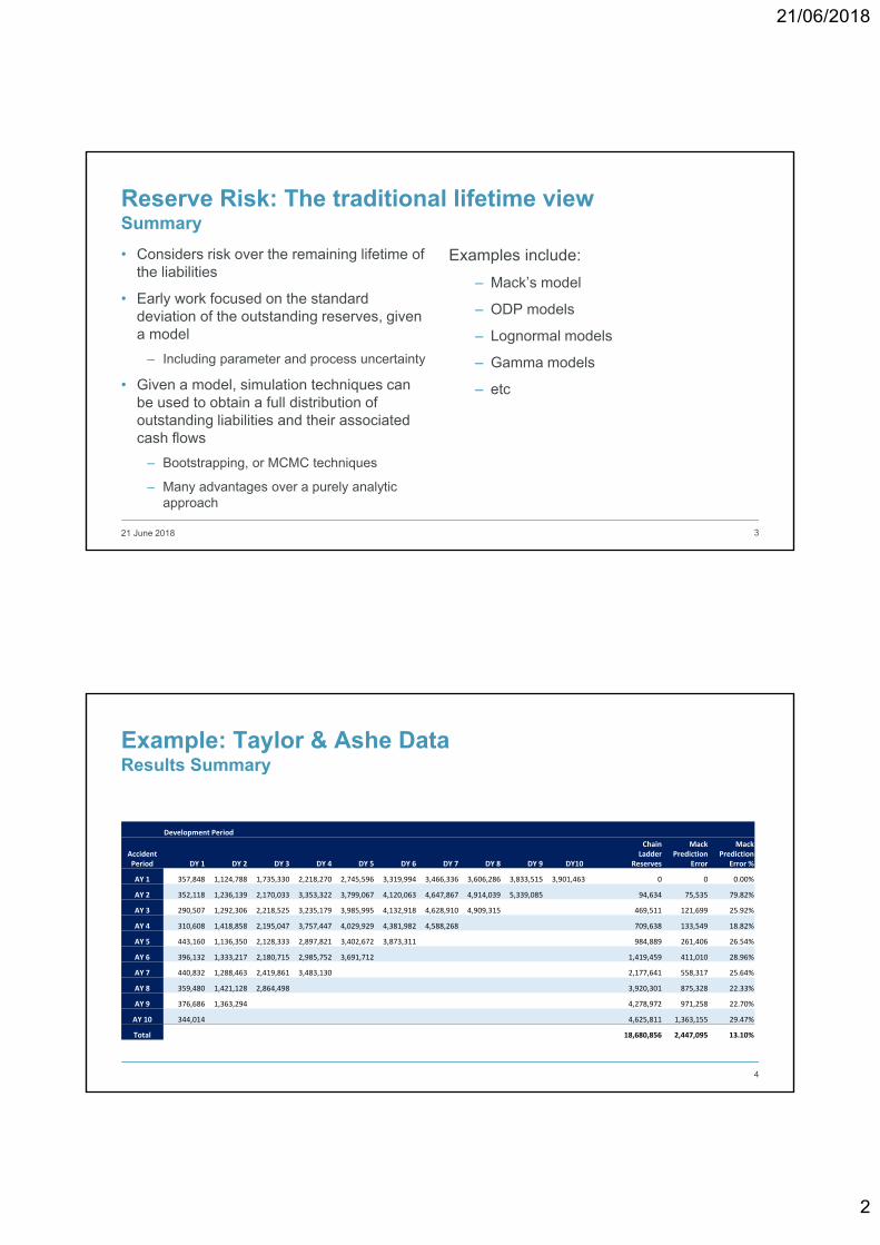
Example: Taylor & Ashe DataResults Summary
4
Development Period
Accident Period DY 1 DY 2 DY 3 DY 4 DY 5 DY 6 DY 7 DY 8 DY 9 DY10
ChainLadder
Reserves
MackPrediction
Error
MackPrediction
Error %
AY 1 357,848 1,124,788 1,735,330 2,218,270 2,745,596 3,319,994 3,466,336 3,606,286 3,833,515 3,901,463 0 0 0.00%
AY 2 352,118 1,236,139 2,170,033 3,353,322 3,799,067 4,120,063 4,647,867 4,914,039 5,339,085 94,634 75,535 79.82%
AY 3 290,507 1,292,306 2,218,525 3,235,179 3,985,995 4,132,918 4,628,910 4,909,315 469,511 121,699 25.92%
AY 4 310,608 1,418,858 2,195,047 3,757,447 4,029,929 4,381,982 4,588,268 709,638 133,549 18.82%
AY 5 443,160 1,136,350 2,128,333 2,897,821 3,402,672 3,873,311 984,889 261,406 26.54%
AY 6 396,132 1,333,217 2,180,715 2,985,752 3,691,712 1,419,459 411,010 28.96%
AY 7 440,832 1,288,463 2,419,861 3,483,130 2,177,641 558,317 25.64%
AY 8 359,480 1,421,128 2,864,498 3,920,301 875,328 22.33%
AY 9 376,686 1,363,294 4,278,972 971,258 22.70%
AY 10 344,014 4,625,811 1,363,155 29.47%
Total 18,680,856 2,447,095 13.10%
21/06/2018
3
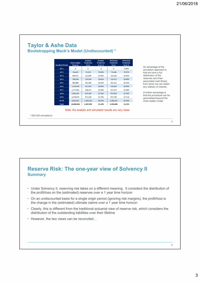
Taylor & Ashe DataBootstrapping Mack’s Model (Undiscounted) *
5
Accident PeriodChain Ladder
Reserve
Analytic Prediction
Error
Analytic PredictionError %
BootstrapPrediction
Error
BootstrapPredictionError %
AY 1 0 0 0 0 0.00%
AY 2 94,634 75,535 79.82% 75,648 79.97%
AY 3 469,511 121,699 25.92% 121,622 25.92%
AY 4 709,638 133,549 18.82% 133,411 18.80%
AY 5 984,889 261,406 26.54% 261,311 26.53%
AY 6 1,419,459 411,010 28.96% 410,643 28.94%
AY 7 2,177,641 558,317 25.64% 557,417 25.58%
AY 8 3,920,301 875,328 22.33% 875,944 22.34%
AY 9 4,278,972 971,258 22.70% 971,783 22.71%
AY 10 4,625,811 1,363,155 29.47% 1,366,322 29.54%
Total 18,680,856 2,447,095 13.10% 2,450,608 13.12%
Note: the analytic and simulated results are very close
An advantage of the simulation approach is that we have a full distribution of the reserves (and their associated cash-flows), from which we can obtain any statistic of interest.
A further advantage is that the procedure can be generalised beyond the chain ladder model
* 500,000 simulations
Reserve Risk: The one-year view of Solvency IISummary
• Under Solvency II, reserving risk takes on a different meaning. It considers the distribution of the profit/loss on the (estimated) reserves over a 1 year time horizon
• On an undiscounted basis for a single origin period (ignoring risk margins), the profit/loss is the change in the (estimated) ultimate claims over a 1 year time horizon
• Clearly, this is different from the traditional actuarial view of reserve risk, which considers the distribution of the outstanding liabilities over their lifetime
• However, the two views can be reconciled…
6
21/06/2018
4
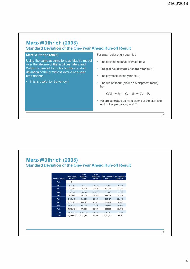
Merz-Wüthrich (2008)
Using the same assumptions as Mack’s model over the lifetime of the liabilities, Merz and Wüthrich derived formulae for the standard deviation of the profit/loss over a one-year time horizon
• This is useful for Solvency II
Merz-Wüthrich (2008)Standard Deviation of the One-Year Ahead Run-off Result
For a particular origin year, let:
• The opening reserve estimate be
• The reserve estimate after one year be
• The payments in the year be
• The run-off result (claims development result) be:
• Where estimated ultimate claims at the start and end of the year are and
7
Merz-Wüthrich (2008)Standard Deviation of the One-Year Ahead Run-off Result
8
Accident PeriodChain Ladder
Reserve
Mack Prediction
Error
Mack PredictionError %
Merz‐Wüthrich RMSEP
Merz‐Wüthrich RMSEP %
AY 1 0
AY 2 94,634 75,535 79.82% 75,535 79.82%
AY 3 469,511 121,699 25.92% 105,309 22.43%
AY 4 709,638 133,549 18.82% 79,846 11.25%
AY 5 984,889 261,406 26.54% 235,115 23.87%
AY 6 1,419,459 411,010 28.96% 318,427 22.43%
AY 7 2,177,641 558,317 25.64% 361,089 16.58%
AY 8 3,920,301 875,328 22.33% 629,681 16.06%
AY 9 4,278,972 971,258 22.70% 588,662 13.76%
AY 10 4,625,811 1,363,155 29.47% 1,029,925 22.26%
Total 18,680,856 2,447,095 13.10% 1,778,968 9.52%
21/06/2018
5
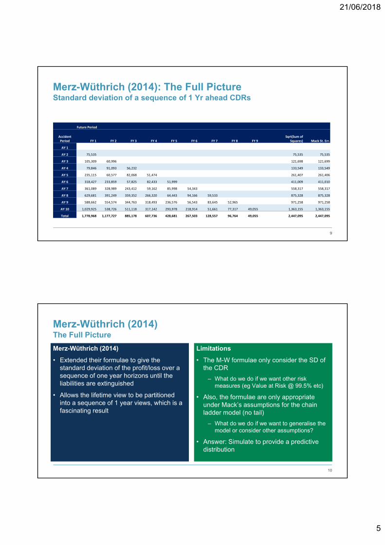
Merz-Wüthrich (2014): The Full PictureStandard deviation of a sequence of 1 Yr ahead CDRs
9
Future Period
Accident Period FY 1 FY 2 FY 3 FY 4 FY 5 FY 6 FY 7 FY 8 FY 9
Sqrt(Sum of Squares) Mack St. Err.
AY 1
AY 2 75,535 75,535 75,535
AY 3 105,309 60,996 121,698 121,699
AY 4 79,846 91,093 56,232 133,549 133,549
AY 5 235,115 60,577 82,068 51,474 261,407 261,406
AY 6 318,427 233,859 57,825 82,433 51,999 411,009 411,010
AY 7 361,089 328,989 243,412 59,162 85,998 54,343 558,317 558,317
AY 8 629,681 391,249 359,352 266,320 64,443 94,166 59,533 875,328 875,328
AY 9 588,662 554,574 344,763 318,493 236,576 56,543 83,645 52,965 971,258 971,258
AY 10 1,029,925 538,726 511,118 317,142 293,978 218,914 51,661 77,317 49,055 1,363,155 1,363,155
Total 1,778,968 1,177,727 885,178 607,736 428,681 267,503 128,557 96,764 49,055 2,447,095 2,447,095
Merz-Wüthrich (2014)The Full Picture
Merz-Wüthrich (2014)
• Extended their formulae to give the standard deviation of the profit/loss over a sequence of one year horizons until the liabilities are extinguished
• Allows the lifetime view to be partitioned into a sequence of 1 year views, which is a fascinating result
Limitations
• The M-W formulae only consider the SD of the CDR
– What do we do if we want other risk measures (eg Value at Risk @ 99.5% etc)
• Also, the formulae are only appropriate under Mack’s assumptions for the chain ladder model (no tail)
– What do we do if we want to generalise the model or consider other assumptions?
• Answer: Simulate to provide a predictive distribution
10
21/06/2018
6
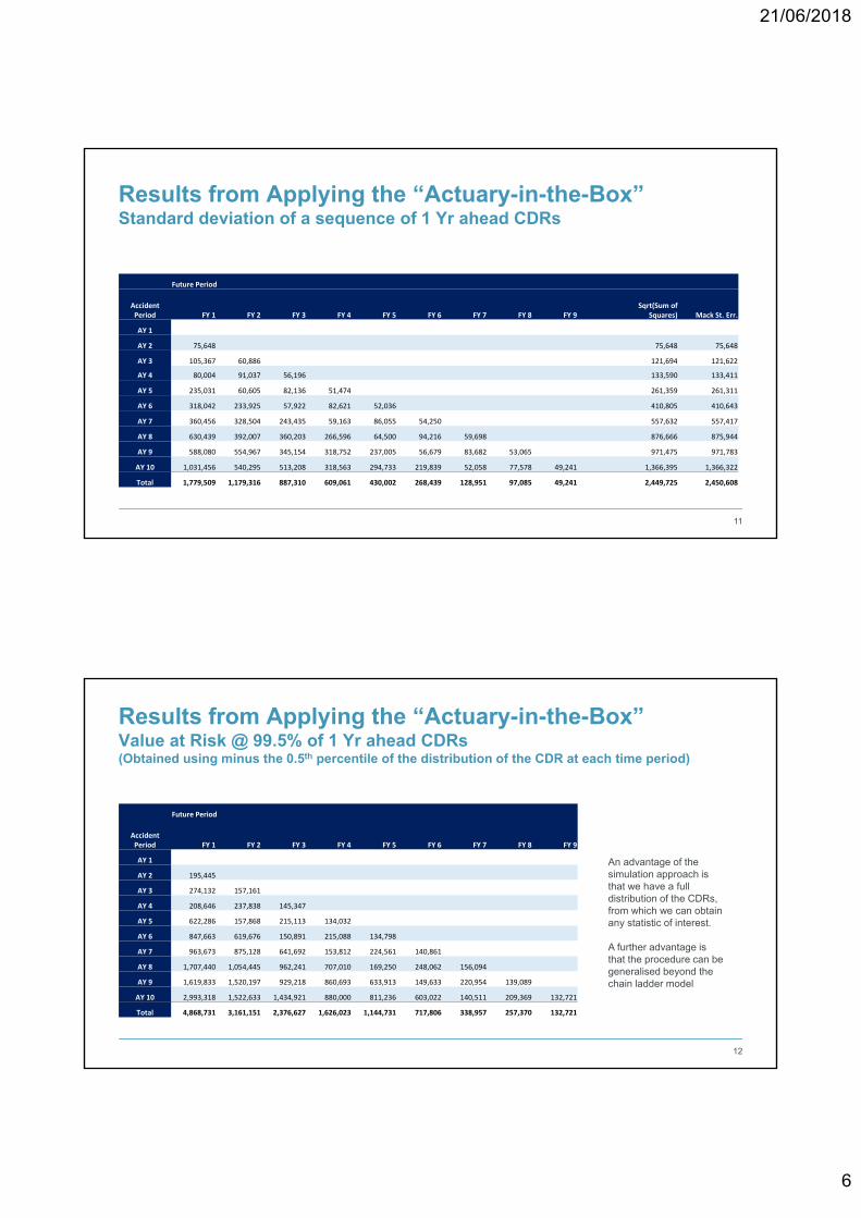
Results from Applying the “Actuary-in-the-Box”Standard deviation of a sequence of 1 Yr ahead CDRs
11
Future Period
Accident Period FY 1 FY 2 FY 3 FY 4 FY 5 FY 6 FY 7 FY 8 FY 9
Sqrt(Sum of Squares) Mack St. Err.
AY 1
AY 2 75,648 75,648 75,648
AY 3 105,367 60,886 121,694 121,622
AY 4 80,004 91,037 56,196 133,590 133,411
AY 5 235,031 60,605 82,136 51,474 261,359 261,311
AY 6 318,042 233,925 57,922 82,621 52,036 410,805 410,643
AY 7 360,456 328,504 243,435 59,163 86,055 54,250 557,632 557,417
AY 8 630,439 392,007 360,203 266,596 64,500 94,216 59,698 876,666 875,944
AY 9 588,080 554,967 345,154 318,752 237,005 56,679 83,682 53,065 971,475 971,783
AY 10 1,031,456 540,295 513,208 318,563 294,733 219,839 52,058 77,578 49,241 1,366,395 1,366,322
Total 1,779,509 1,179,316 887,310 609,061 430,002 268,439 128,951 97,085 49,241 2,449,725 2,450,608
Results from Applying the “Actuary-in-the-Box”Value at Risk @ 99.5% of 1 Yr ahead CDRs(Obtained using minus the 0.5th percentile of the distribution of the CDR at each time period)
12
Future Period
Accident Period FY 1 FY 2 FY 3 FY 4 FY 5 FY 6 FY 7 FY 8 FY 9
AY 1
AY 2 195,445
AY 3 274,132 157,161
AY 4 208,646 237,838 145,347
AY 5 622,286 157,868 215,113 134,032
AY 6 847,663 619,676 150,891 215,088 134,798
AY 7 963,673 875,128 641,692 153,812 224,561 140,861
AY 8 1,707,440 1,054,445 962,241 707,010 169,250 248,062 156,094
AY 9 1,619,833 1,520,197 929,218 860,693 633,913 149,633 220,954 139,089
AY 10 2,993,318 1,522,633 1,434,921 880,000 811,236 603,022 140,511 209,369 132,721
Total 4,868,731 3,161,151 2,376,627 1,626,023 1,144,731 717,806 338,957 257,370 132,721
An advantage of the simulation approach is that we have a full distribution of the CDRs, from which we can obtain any statistic of interest.
A further advantage is that the procedure can be generalised beyond the chain ladder model
21/06/2018
7
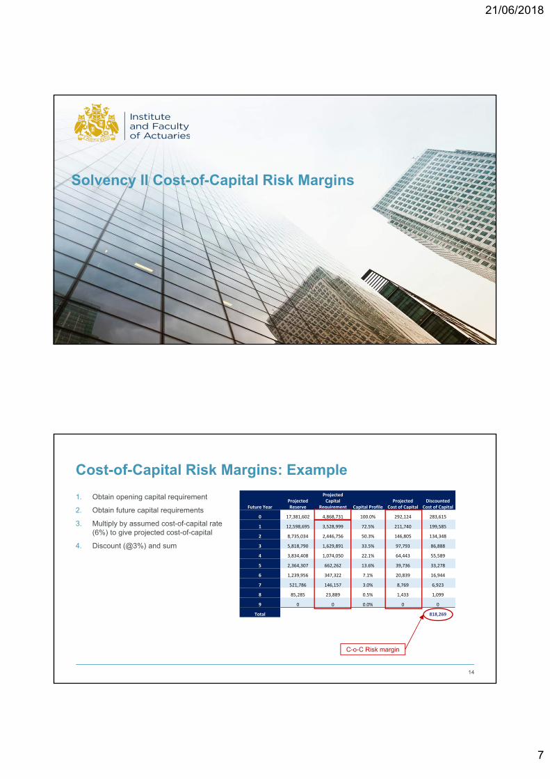
Solvency II Cost-of-Capital Risk Margins
Future YearProjected Reserve
Projected Capital
Requirement Capital ProfileProjected
Cost of CapitalDiscounted
Cost of Capital
0 17,381,602 4,868,731 100.0% 292,124 283,615
1 12,598,695 3,528,999 72.5% 211,740 199,585
2 8,735,034 2,446,756 50.3% 146,805 134,348
3 5,818,790 1,629,891 33.5% 97,793 86,888
4 3,834,408 1,074,050 22.1% 64,443 55,589
5 2,364,307 662,262 13.6% 39,736 33,278
6 1,239,956 347,322 7.1% 20,839 16,944
7 521,786 146,157 3.0% 8,769 6,923
8 85,285 23,889 0.5% 1,433 1,099
9 0 0 0.0% 0 0
Total 818,269
Cost-of-Capital Risk Margins: Example
1. Obtain opening capital requirement
2. Obtain future capital requirements
3. Multiply by assumed cost-of-capital rate (6%) to give projected cost-of-capital
4. Discount (@3%) and sum
14
C-o-C Risk margin
21/06/2018
8
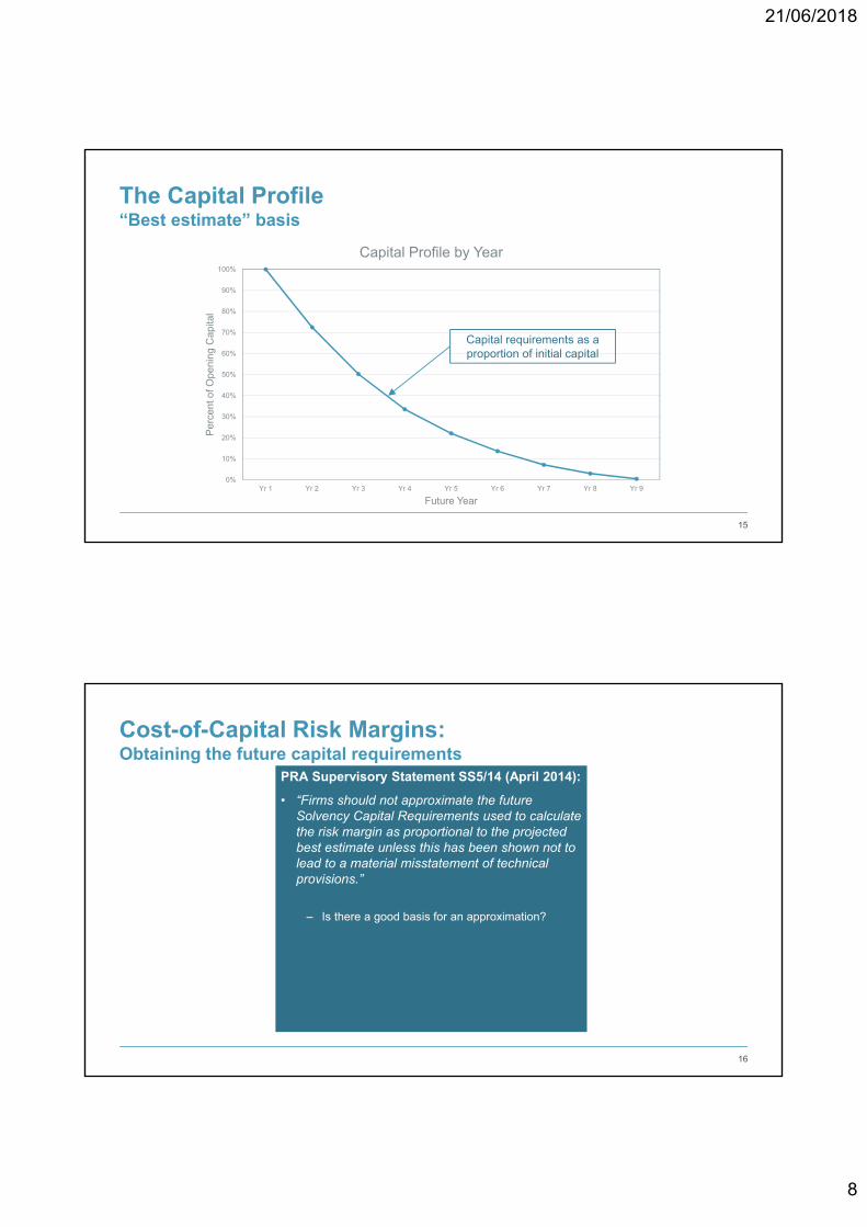
The Capital Profile“Best estimate” basis
15
0%
10%
20%
30%
40%
50%
60%
70%
80%
90%
100%
Yr 1 Yr 2 Yr 3 Yr 4 Yr 5 Yr 6 Yr 7 Yr 8 Yr 9
Pe
rcen
t of O
peni
ng C
apita
l
Future Year
Capital Profile by Year
Capital requirements as a proportion of initial capital
Cost-of-Capital Risk Margins:Obtaining the future capital requirements
16
PRA Supervisory Statement SS5/14 (April 2014):
• “Firms should not approximate the future Solvency Capital Requirements used to calculate the risk margin as proportional to the projected best estimate unless this has been shown not to lead to a material misstatement of technical provisions.”
– Is there a good basis for an approximation?
21/06/2018
9
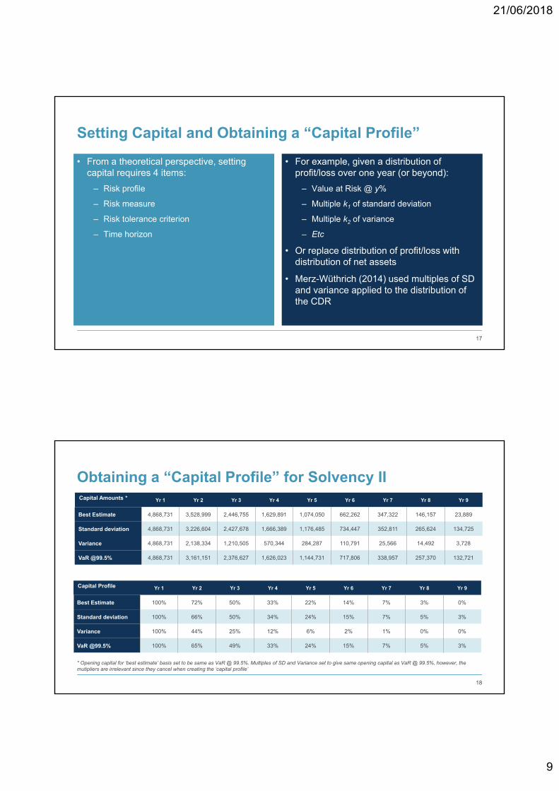
Setting Capital and Obtaining a “Capital Profile”
• From a theoretical perspective, setting capital requires 4 items:
– Risk profile
– Risk measure
– Risk tolerance criterion
– Time horizon
• For example, given a distribution of profit/loss over one year (or beyond):
– Value at Risk @ y%
– Multiple k1 of standard deviation
– Multiple k2 of variance
– Etc
• Or replace distribution of profit/loss with distribution of net assets
• Merz-Wüthrich (2014) used multiples of SD and variance applied to the distribution of the CDR
17
Obtaining a “Capital Profile” for Solvency II
18
Capital Amounts * Yr 1 Yr 2 Yr 3 Yr 4 Yr 5 Yr 6 Yr 7 Yr 8 Yr 9
Best Estimate 4,868,731 3,528,999 2,446,755 1,629,891 1,074,050 662,262 347,322 146,157 23,889
Standard deviation 4,868,731 3,226,604 2,427,678 1,666,389 1,176,485 734,447 352,811 265,624 134,725
Variance 4,868,731 2,138,334 1,210,505 570,344 284,287 110,791 25,566 14,492 3,728
VaR @99.5% 4,868,731 3,161,151 2,376,627 1,626,023 1,144,731 717,806 338,957 257,370 132,721
Capital Profile Yr 1 Yr 2 Yr 3 Yr 4 Yr 5 Yr 6 Yr 7 Yr 8 Yr 9
Best Estimate 100% 72% 50% 33% 22% 14% 7% 3% 0%
Standard deviation 100% 66% 50% 34% 24% 15% 7% 5% 3%
Variance 100% 44% 25% 12% 6% 2% 1% 0% 0%
VaR @99.5% 100% 65% 49% 33% 24% 15% 7% 5% 3%
* Opening capital for ‘best estimate’ basis set to be same as VaR @ 99.5%. Multiples of SD and Variance set to give same opening capital as VaR @ 99.5%, however, the mutipliers are irrelevant since they cancel when creating the ‘capital profile’
21/06/2018
10
19
0%
10%
20%
30%
40%
50%
60%
70%
80%
90%
100%
Yr 1 Yr 2 Yr 3 Yr 4 Yr 5 Yr 6 Yr 7 Yr 8 Yr 9
Percent of Open
ing Capital
Future Year
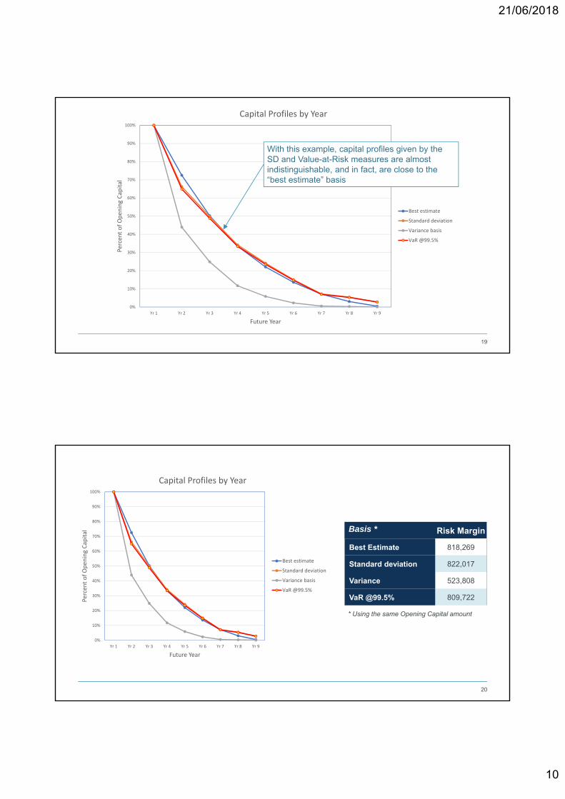
Capital Profiles by Year
Best estimate
Standard deviation
Variance basis
VaR @99.5%
With this example, capital profiles given by the SD and Value-at-Risk measures are almost indistinguishable, and in fact, are close to the “best estimate” basis
20
0%
10%
20%
30%
40%
50%
60%
70%
80%
90%
100%
Yr 1 Yr 2 Yr 3 Yr 4 Yr 5 Yr 6 Yr 7 Yr 8 Yr 9
Percent of Open
ing Capital
Future Year
Capital Profiles by Year
Best estimate
Standard deviation
Variance basis
VaR @99.5%
Basis * Risk Margin
Best Estimate 818,269
Standard deviation 822,017
Variance 523,808
VaR @99.5% 809,722
* Using the same Opening Capital amount
21/06/2018
11
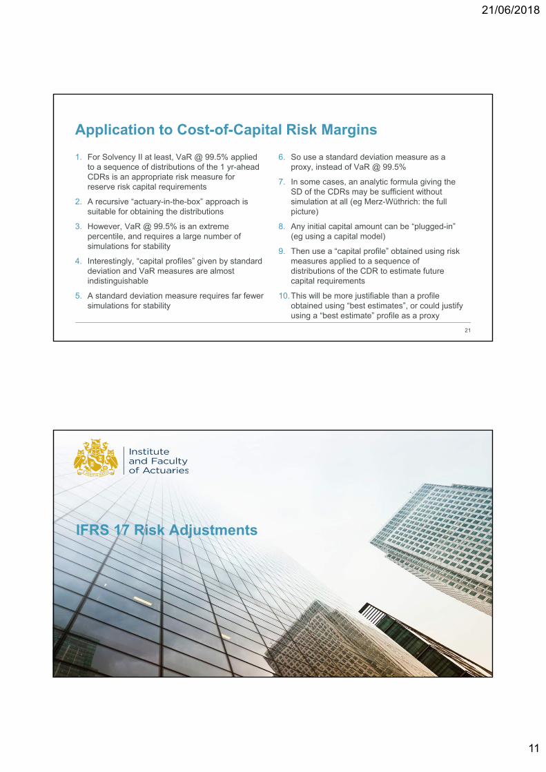
Application to Cost-of-Capital Risk Margins
1. For Solvency II at least, VaR @ 99.5% applied to a sequence of distributions of the 1 yr-ahead CDRs is an appropriate risk measure for reserve risk capital requirements
2. A recursive “actuary-in-the-box” approach is suitable for obtaining the distributions
3. However, VaR @ 99.5% is an extreme percentile, and requires a large number of simulations for stability
4. Interestingly, “capital profiles” given by standard deviation and VaR measures are almost indistinguishable
5. A standard deviation measure requires far fewer simulations for stability
6. So use a standard deviation measure as a proxy, instead of VaR @ 99.5%
7. In some cases, an analytic formula giving the SD of the CDRs may be sufficient without simulation at all (eg Merz-Wüthrich: the full picture)
8. Any initial capital amount can be “plugged-in” (eg using a capital model)
9. Then use a “capital profile” obtained using risk measures applied to a sequence of distributions of the CDR to estimate future capital requirements
10.This will be more justifiable than a profile obtained using “best estimates”, or could justify using a “best estimate” profile as a proxy
21
IFRS 17 Risk Adjustments

21/06/2018
12
Summary
What needs to be done
“An entity shall adjust the estimate of the present value of the future cash flows to reflect the compensation that the entity requires for bearing the uncertainty about the amount and timing of the cash flows that arises from non-financial risk.” (Para 37)
What needs to be disclosed
“An entity shall disclose the confidence level used to determine the risk adjustment for non-financial risk. If the entity uses a technique other than the confidence level technique for determining the risk adjustment for non-financial risk, it shall disclose the technique used and the confidence level corresponding to the results of that technique.” (Para 119)
23
Questions
• Lifetime view or one-year view of Solvency II?
• IFRS 17 mentions a risk measure (confidence level), but what is the risk profile?
• Net or Gross discounted future cash flows (or both)?
• How will reinsurance programmes be taken into account?
• What level of aggregation will be used? Portfolio/legal entity/holding company?
• If calculated at a higher level, how will risk adjustments be allocated back (if required). Will equivalent “confidence levels” be required at a lower level?
• If calculated at a lower level and summed, how will diversification be taken into account in a sensible way, and how will the equivalent “confidence level” be ascertained?
24
21/06/2018
13
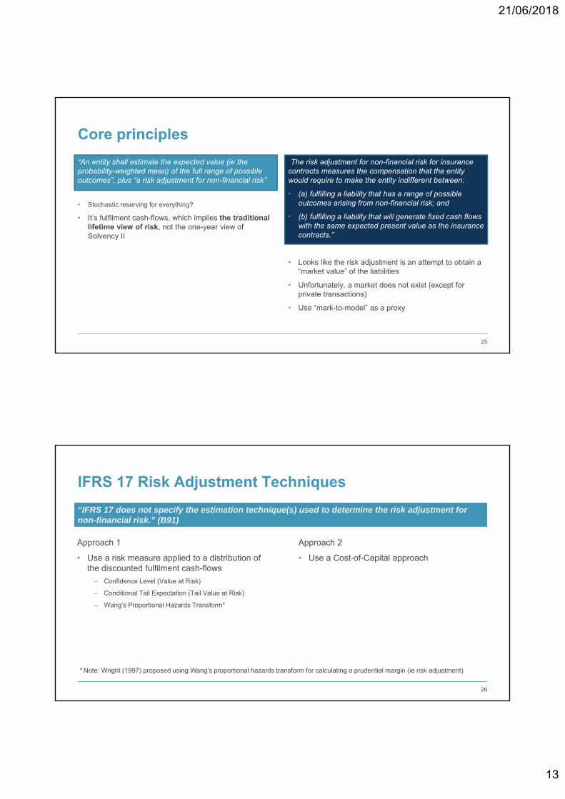
Core principles
“An entity shall estimate the expected value (ie the probability-weighted mean) of the full range of possible outcomes”, plus “a risk adjustment for non-financial risk”
• Stochastic reserving for everything?
• It’s fulfilment cash-flows, which implies the traditional lifetime view of risk, not the one-year view of Solvency II
“The risk adjustment for non-financial risk for insurance contracts measures the compensation that the entity would require to make the entity indifferent between:
• (a) fulfilling a liability that has a range of possible outcomes arising from non-financial risk; and
• (b) fulfilling a liability that will generate fixed cash flows with the same expected present value as the insurance contracts.”
• Looks like the risk adjustment is an attempt to obtain a “market value” of the liabilities
• Unfortunately, a market does not exist (except for private transactions)
• Use “mark-to-model” as a proxy
25
IFRS 17 Risk Adjustment Techniques
Approach 1
• Use a risk measure applied to a distribution of the discounted fulfilment cash-flows
– Confidence Level (Value at Risk)
– Conditional Tail Expectation (Tail Value at Risk)
– Wang’s Proportional Hazards Transform*
26
“IFRS 17 does not specify the estimation technique(s) used to determine the risk adjustment for non-financial risk.” (B91)
Approach 2
• Use a Cost-of-Capital approach
* Note: Wright (1997) proposed using Wang’s proportional hazards transform for calculating a prudential margin (ie risk adjustment)
21/06/2018
14
IFRS 17 Risk Adjustment Techniques
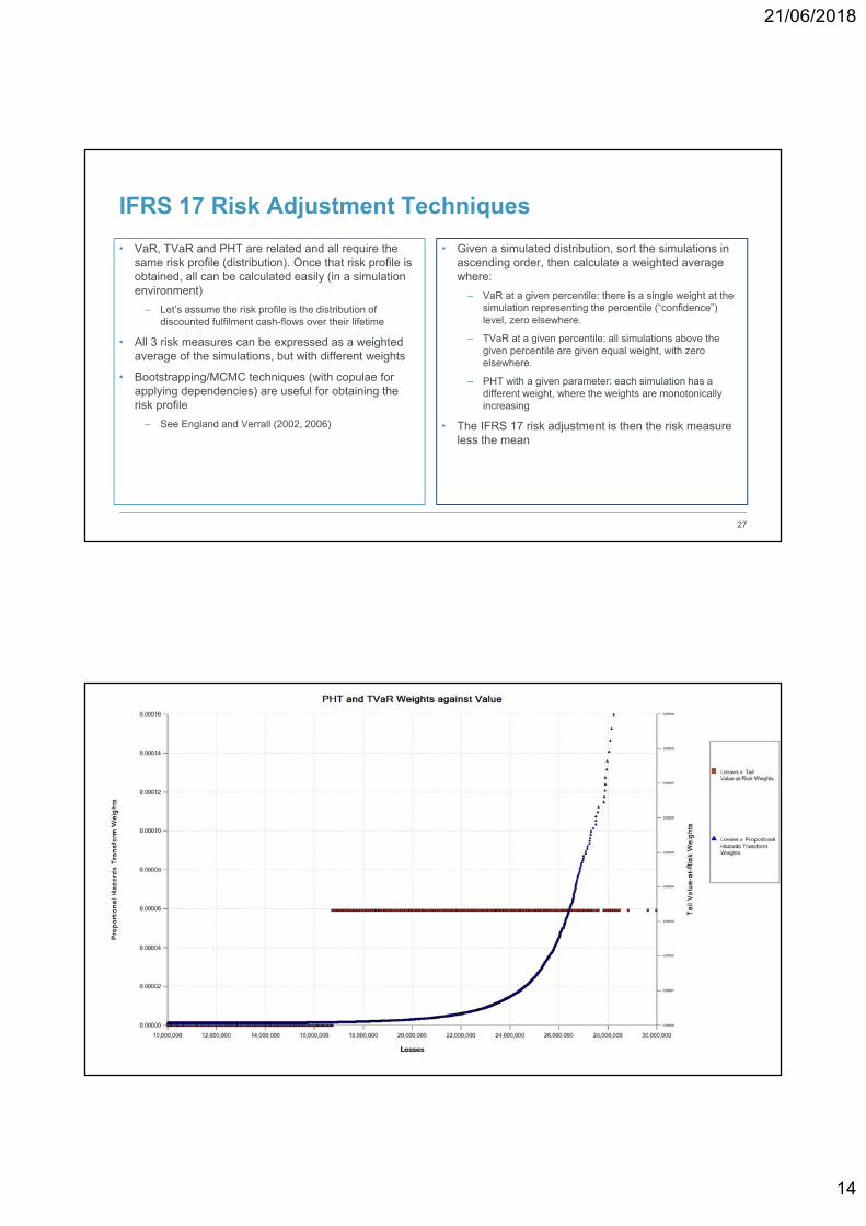
• VaR, TVaR and PHT are related and all require the same risk profile (distribution). Once that risk profile is obtained, all can be calculated easily (in a simulation environment)
– Let’s assume the risk profile is the distribution of discounted fulfilment cash-flows over their lifetime
• All 3 risk measures can be expressed as a weighted average of the simulations, but with different weights
• Bootstrapping/MCMC techniques (with copulae for applying dependencies) are useful for obtaining the risk profile
– See England and Verrall (2002, 2006)
• Given a simulated distribution, sort the simulations in ascending order, then calculate a weighted average where:
– VaR at a given percentile: there is a single weight at the simulation representing the percentile (“confidence”) level, zero elsewhere.
– TVaR at a given percentile: all simulations above the given percentile are given equal weight, with zero elsewhere.
– PHT with a given parameter: each simulation has a different weight, where the weights are monotonically increasing
• The IFRS 17 risk adjustment is then the risk measure less the mean
27
Graphs of TVaR and PHT weights
21 June 2018 28
21/06/2018
15
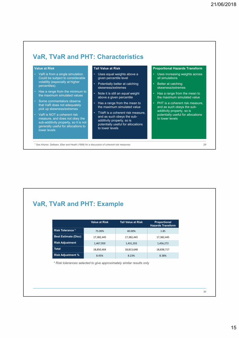
VaR, TVaR and PHT: Characteristics
Value at Risk
• VaR is from a single simulation. Could be subject to considerable volatility (especially at higher percentiles).
• Has a range from the minimum to the maximum simulated values
• Some commentators observe that VaR does not adequately pick up skewness/extremes
• VaR is NOT a coherent risk measure, and does not obey the sub-additivity property, so it is not generally useful for allocations to lower levels
Proportional Hazards Transform
• Uses increasing weights across all simulations
• Better at catching skewness/extremes
• Has a range from the mean to the maximum simulated value
• PHT is a coherent risk measure, and as such obeys the sub-additivity property, so is potentially useful for allocations to lower levels
29
Tail Value at Risk
• Uses equal weights above a given percentile level
• Potentially better at catching skewness/extremes
• Note it is still an equal weight above a given percentile
• Has a range from the mean to the maximum simulated value
• TVaR is a coherent risk measure, and as such obeys the sub-additivity property, so is potentially useful for allocations to lower levels
* See Artzner, Delbaen, Eber and Heath (1999) for a discussion of coherent risk measures
VaR, TVaR and PHT: Example
30
Value at Risk Tail Value at Risk Proportional Hazards Transform
Risk Tolerance * 75.00% 40.00% 1.85
Best Estimate (Disc) 17,382,445 17,382,445 17,382,445
Risk Adjustment 1,467,959 1,431,203 1,456,272
Total 18,850,404 18,813,648 18,838,717
Risk Adjustment % 8.45% 8.23% 8.38%
* Risk tolerances selected to give approximately similar results only
21/06/2018
16
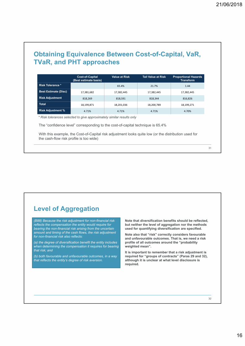
Obtaining Equivalence Between Cost-of-Capital, VaR, TVaR, and PHT approaches
31
Cost-of-Capital(Best estimate basis)
Value at Risk Tail Value at Risk Proportional Hazards Transform
Risk Tolerance * 65.4% 21.7% 1.44
Best Estimate (Disc) 17,381,682 17,382,445 17,382,445 17,382,445
Risk Adjustment 818,269 818,591 818,344 816,826
Total 18,199,871 18,201,036 18,200,789 18,199,271
Risk Adjustment % 4.71% 4.71% 4.71% 4.70%
* Risk tolerances selected to give approximately similar results only
The “confidence level” corresponding to the cost-of-capital technique is 65.4%
With this example, the Cost-of-Capital risk adjustment looks quite low (or the distribution used for the cash-flow risk profile is too wide)
Level of Aggregation
(B88) Because the risk adjustment for non-financial risk reflects the compensation the entity would require for bearing the non-financial risk arising from the uncertain amount and timing of the cash flows, the risk adjustment for non-financial risk also reflects:
(a) the degree of diversification benefit the entity includes when determining the compensation it requires for bearing that risk; and
(b) both favourable and unfavourable outcomes, in a way that reflects the entity’s degree of risk aversion.
Note that diversification benefits should be reflected, but neither the level of aggregation nor the methods used for quantifying diversification are specified.
Note also that “risk” correctly considers favourable and unfavourable outcomes. That is, we need a risk profile of all outcomes around the “probability weighted mean”.
It is important to remember that a risk adjustment is required for “groups of contracts” (Paras 29 and 32), although it is unclear at what level disclosure is required.
32
21/06/2018
17
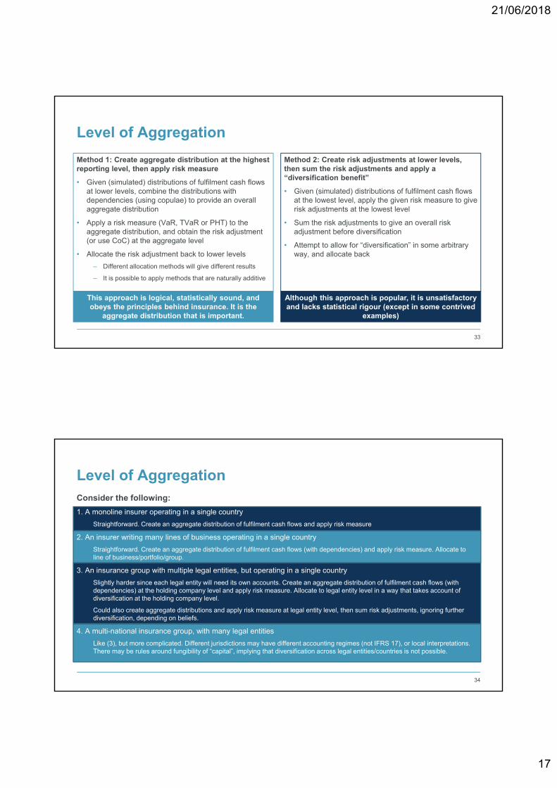
Level of Aggregation
Method 1: Create aggregate distribution at the highest reporting level, then apply risk measure
• Given (simulated) distributions of fulfilment cash flows at lower levels, combine the distributions with dependencies (using copulae) to provide an overall aggregate distribution
• Apply a risk measure (VaR, TVaR or PHT) to the aggregate distribution, and obtain the risk adjustment (or use CoC) at the aggregate level
• Allocate the risk adjustment back to lower levels
– Different allocation methods will give different results
– It is possible to apply methods that are naturally additive
Method 2: Create risk adjustments at lower levels, then sum the risk adjustments and apply a “diversification benefit”
• Given (simulated) distributions of fulfilment cash flows at the lowest level, apply the given risk measure to give risk adjustments at the lowest level
• Sum the risk adjustments to give an overall risk adjustment before diversification
• Attempt to allow for “diversification” in some arbitrary way, and allocate back
33
This approach is logical, statistically sound, and obeys the principles behind insurance. It is the
aggregate distribution that is important.
Although this approach is popular, it is unsatisfactory and lacks statistical rigour (except in some contrived
examples)
Consider the following:
1. A monoline insurer operating in a single country
Straightforward. Create an aggregate distribution of fulfilment cash flows and apply risk measure
2. An insurer writing many lines of business operating in a single country
Straightforward. Create an aggregate distribution of fulfilment cash flows (with dependencies) and apply risk measure. Allocate to line of business/portfolio/group.
3. An insurance group with multiple legal entities, but operating in a single country
Slightly harder since each legal entity will need its own accounts. Create an aggregate distribution of fulfilment cash flows (with dependencies) at the holding company level and apply risk measure. Allocate to legal entity level in a way that takes account ofdiversification at the holding company level.
Could also create aggregate distributions and apply risk measure at legal entity level, then sum risk adjustments, ignoring further diversification, depending on beliefs.
4. A multi-national insurance group, with many legal entities
Like (3), but more complicated. Different jurisdictions may have different accounting regimes (not IFRS 17), or local interpretations. There may be rules around fungibility of “capital”, implying that diversification across legal entities/countries is not possible.
Level of Aggregation
34
21/06/2018
18
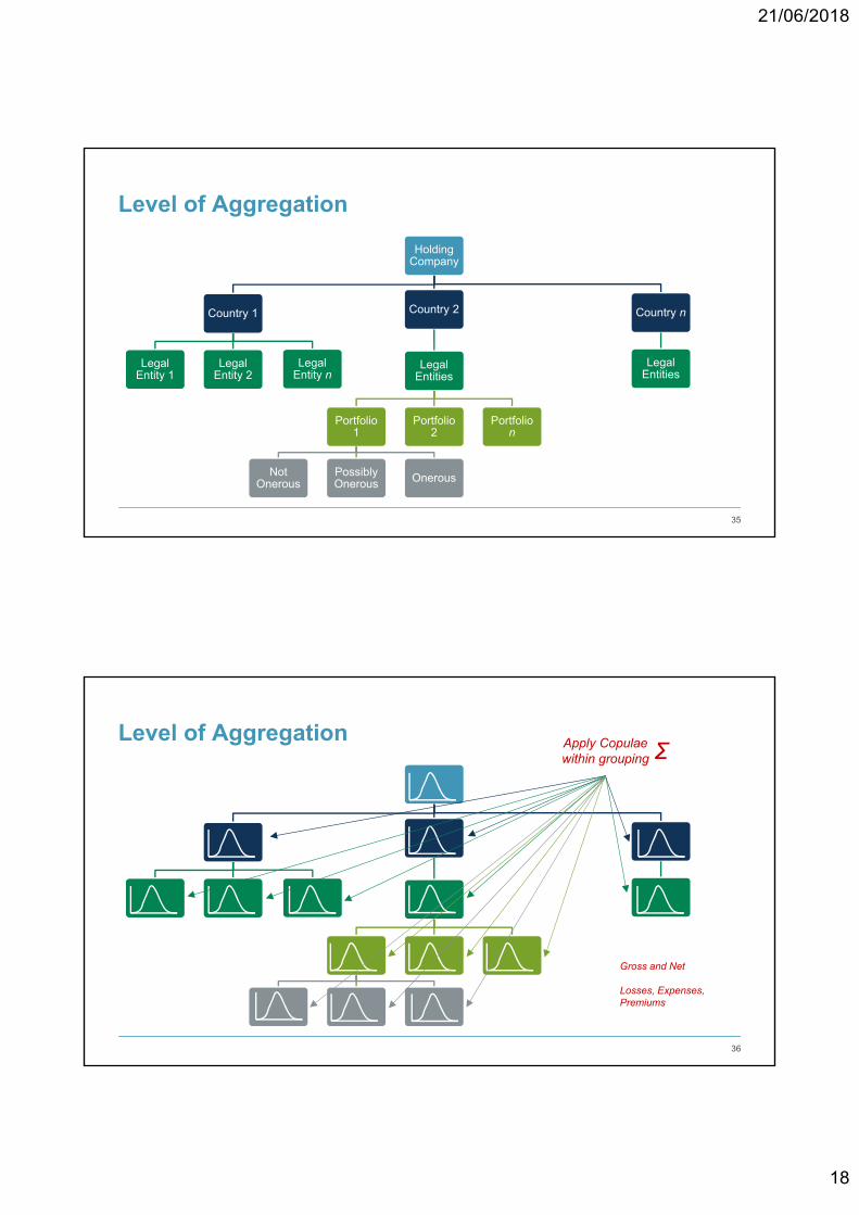
Level of Aggregation
Holding Company
Country 1
Legal Entity 1
Legal Entity 2
Legal Entity n
Country 2
Legal Entities
Portfolio 1
Not Onerous
Possibly Onerous Onerous
Portfolio 2
Portfolio n
Country n
Legal Entities
35
Level of Aggregation
36
Apply Copulaewithin grouping Σ
Gross and Net
Losses, Expenses, Premiums
21/06/2018
19
Reinsurance
• An explicit risk adjustment for reinsurance is required
– Calculate using distribution of reinsurance cash-flows, or use gross and net distributions of the underlying and take the difference?
– Either way, a distribution of the reinsurance cash-flows is required
• This hints at modelling the reinsurance programmes, contract by contract, year of account by year of account
• Modelling all reinsurance programmes could be a lot of work, and requires individual claims data
• The traditional approach of using aggregate gross triangles and simulating an approximate net to gross ratio looks increasingly inadequate
Reinsurance modelling for risk adjustments?
• Use triangle approaches (eg bootstrapping) for attritional claims
• Develop open large claims (and claims that could become large) to their ultimate position stochastically
• Obtain cash-flows for the development of large claims
• Pass simulated large claims through the non-proportional reinsurance programmes (quota share is easy) and net down
• Take care over aggregates etc for which knowledge of the sum of existing closed claims is required
• Remember re-instatement premiums
• Obtain total reinsurance cashflows across all contracts and years of account, and subtract from gross cash-flow distributions to obtain a net distribution
37
Conclusions
• Approaches to estimating the risk adjustment under IFRS 17 using a risk measure applied to the distribution of fulfilment cash flows are straightforward to apply
– Given a distribution of the fulfilment cash flows, select a risk measure and risk tolerance level
• The cost-of-capital method is more complex and requires additional variables, assumptions, and sensitivities
– Opening capital requirement
– Future capital requirements
– Cost of capital rate
– Discount rate
• Note that under IFRS 17, the time horizon for capital is the lifetime of the fulfilment cash flows.
– This is different from Solvency II, so Solvency II risk margins should not be used for IFRS 17
– See England, Verrall and Wüthrich (2018)
• Under IFRS 17, the equivalent “confidence level” has to be disclosed anyway, so why bother with the “Cost-of-Capital” approach at all?
• Reinsurance and issues around aggregation and diversification introduce significant challenges
21 June 2018 38

21/06/2018
20
References
• Artzner, P, Delbaen, F, Eber, J-M and Heath, D (1999). Coherent Measures of Risk. Mathematical Finance, 9, 203–228
• England, PD and Verrall, RJ (2002). Stochastic Claims Reserving in General Insurance. British Actuarial Journal, 8, 443-544
• England, PD and Verrall, RJ (2006). Predictive Distributions of Outstanding Liabilities in General Insurance. Annals of Actuarial Science, 1, II, 221-270
• England, PD, Verrall, RJ, and Wüthrich, MV (2018). On the Lifetime and One-Year Views of Reserve Risk, with Application to IFRS 17 and Solvency II Risk Margins. Available at SSRN: https://ssrn.com/abstract=3141239
• International Actuarial Association (2016). Risk Adjustments for Financial Reporting of Insurance Contracts Under International Financial Reporting Standards No. X. Educational Monograph (Exposure Draft).
• Mack, T (1993). Distribution-free calculation of the standard error of chain-ladder reserve estimates. ASTIN Bulletin, 22, 93-109
• Merz, M and Wüthrich, MV (2008). Modelling the claims development result for solvency purposes. CAS E-Forum Fall 2008, 542-568
• Merz, M and Wüthrich, MV (2014) Claims Run-Off Uncertainty: The Full Picture. Swiss Finance Institute Research Paper No. 14-69. Available at SSRN: https://ssrn.com/abstract=2524352.
• Wang, S (1995). Insurance Pricing and Increased Limits Ratemaking by Proportional Hazards Transforms. Insurance Mathematics and Economics, 17, 43–54
• Wang, S (1998). Implementation of Proportional Hazards Transforms in Ratemaking. Proceedings of the Casualty Actuarial Society, LXXXV, 940-979
• Wright, T.S. (1997). Probability Distribution of Outstanding Liability from Individual Payments Data. Claims Reserving Manual, 2, Institute of Actuaries
39
EMC Actuarial & Analytics
21 June 2018 40
Peter England
– Capital
– Reserving
– IFRS 17
– Stochastic/statistical modelling
– Research
Matthew Evans
– Pricing
– Reserving
– Data Science
– InsurTech

21/06/2018
21
21 June 2018 41
Questions Comments
The views expressed in this presentation are the current views of the author and not necessarily those of the IFoA. The IFoA do not endorse any of the views stated, nor any claims or representations made in this presentation and accept no responsibility or liability to any person for loss or damage suffered as a consequence of their placing reliance upon any view, claim or representation made in this presentation.
The information and expressions of opinion contained in this presentation are not intended to be a comprehensive study, nor to provide actuarial advice or advice of any nature and should not be treated as a substitute for specific advice concerning individual situations. On no account may any part of this presentation be reproduced without the written permission of the authors.
The author reserves the right to change their minds at a future date.