ON THE PROBLEM OF MATCHING LISTS BY SAMPLES

W. EDWARDS DEMING

AND

GERALD J. GLASSER

NEW YORK U I ~ B L E S ~ Y

, OB THE

Val. 519,

ON THE PROBLEM OF MATCHING LISTS BY SAMPLES

W. EDWA~DS DEMING AND GERALD J. GLASSER New Yorlc University

This paper presents theory for estimation of the proportions of names common to two or more lists of names, through use of samples drawn from the lists. The theory covers (a) the probability distributions, ex- pected values, variances, and the third and fourth moments of the estimates of the proportions duplicated; (b) testing a hypothesis with respect to a proportion; (c) optimum allocation of the samples; (d) the, effect of duplicates within a list; (e) possible gains from stratification. Examples illustrate some of the theory.

S TATEMENT of the problem. There are 2 or more long lists of names. Some names may be common to some or all of the lists, and it is of some economic

or scientific importance to discover how many. The lists may be very long: in practice they may run to several hundred thousand or millions of names. One example came up in Germany a few years ago where the government wished to know how many people receive regular cheques from several sourcesfor exam- ple, government payroll, social security, unemployment compensation, subsidy of one kind or another, ex-soldier's allowance, and possibly other sources. An- other example is provided by a publisher of a magazine who wished to discover how many of his subscribers were on a list of executives, and on other special lists.

An advertising agency or the marketing department of a firm must decide whether to use one or both of 2 lists of names available to them for an advertis- ing campaign. The number of names common to both lists would be, if they knew it, the key decision-parameter. A firm may wish to determine, by com- paring two lists, how many of their present employees worked there in some past year. The number of shareholders common to two or more companies, and the number of companies that do business in each of two states, are addi- tional problems which require the matching of lists. Library work affords other illustrations. This paper presents some statistical theory for the solution of such problems.

Several of the results (including estimators for relevant parameters and approx- imations to their variances) have already appeared in a note by Goodman.' Here we apply and extend his work.

The theory that we give here, like Goodman's, is based on probability sam- ples from both lists. Incidentally, a sample from one list matched against the other in full (100%) presents only a simple case of random sampling from a finite population of attributes; it is also a limiting case of the general theory of mtching two samples.

Notdim. The accompanying table shows the scheme of notation. al, a*, . . + , a~ are distinct and ordered names on one list; bl, bz, - - , b~ are distinct and

, ordered names on the other list. D names are common to both lists. We assume : that no name appears more than once on one list; however, we illustrate later

1 Qoodmsn, Zeo A., .On the analyaia of aamplea from k lists," Annola of MaUlandied Sfdistics, %3 (186S, m-

403

404 AMERICAN STATISTICAL ASSOCIATION JOURNAL, JUNE 1969

the relaxation of this requirement. The number D is important: it is the number that the publisher (for example) wishes to know. Let

It will suffice to estimate either p or P.

The comparison of name a; in List 1 with name bj in List 2 gives

aibi = 1 if the 2 names are identical

= 0 otherwise.

Number on the list Number common to both lists Proportion oommon to both lists

Then the number D of names common to both lists is

C = D (4)

where i in the summation runs through List 1, and j runs through List 2. Let names in the samples be

XI, x , , from List 1

YI, ~ / a , . . . , yn from List 2

{ siyj = 1 if the 2 names are identical

= 0 otherwise.

We also define

d = x x , y j ~ i = 1 , 2 , - . - , m ; j = 1 , 2 , . . . , n ]

the number of names common to the 2 samples. d is a random variable.

Sampling procedu.re

List 1

a1 UP

ai

ax

M D P

(1) Draw by random numbers between 1 and M and without replacement m names from List 1.

(2) Draw by random numbers between 1 and N and without replacement n names from List 2.

List 2

bl b2

ba

b~

N D P

MATCHING LISTS BY SAMPLES 405

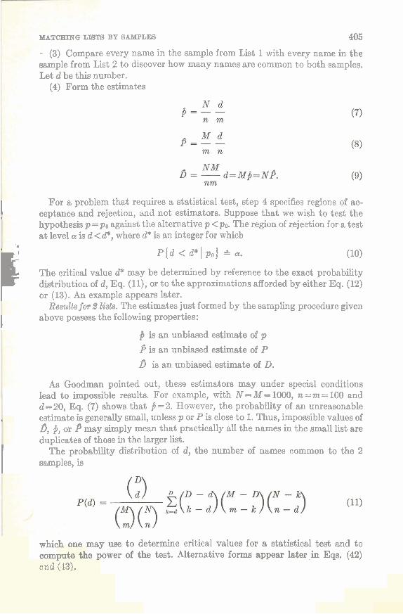
(3) Compare every name in the sample from List 1 with every name in the sample from List 2 to discover how many names are common to both samples. Let d be this number.

(4) Form the estimates

I For a problem that requires a statistical test, step 4 specifies regions of ac- ceptance and rejection, and not estimators. Suppose that we wish to test the hypothesis p=po against the alternative p <PO. The region of rejection for a test a t level a is d <d*, where d* is an integer for which r ~ { d < d*Ip,) a. (10)

The critical value d* may be determined by reference to the exact probability distribution of d, Eq. ( l l ) , or to the approximations afforded by either Eq. (12) or (13). An example appears later.

Resultsfor d lists. The estimates just formed by the sampling procedure given

I above possess the following properties:

is an unbiased estimate of p

P is an unbiased estimate of P

fi is an unbiased estimate of D.

As Goodman pointed out, these estimators may under special conditions lead to impossible results. For example, with N = M = 1000, n = m = 100 and d=20, Eq. (7) shows that $ =2. However, the probability of an unreasonable estimate is generally small, unless p or P is close to 1. Thus, impossible values of B, j, or P may simply mean that practically all the names in the small list are duplicates of those in the larger list.

I The probability distribution of d, the number of names common to the 2 samples, is

which one may use to determine critical values for a statistical test and to compute fhe power of the test. Alternative forms appear later in Eqs. (42) cnC! (13).

AMERICAN STATISTICAL ASSOCIATION JOURNAL, JUNE 1969

We introduce 2 limiting cases. Case 1: M, N, m, n all increase without limit in such manner that D, m/M, n/N remain fked. Case 2: M, N, m, n, and D all increase without limit in such manner that mnD/MN remains fixed a t the value A. In Case 1

where f = mn/MN. The Limit in Case 1 is obviously a binomial with parameters D and f. It is comparable to the binomial limit for the hypergeometric distri- bution? I t gives a good approximation to the exact distribution Eq. (11) if M, N, m, and n are reasonably large. In Case 2

which is a Poisson distribution. This equation also approximates the exact distribution in Eq. (11) iff is small. In addition

Case 2.

If the sample from List 2 is complete, then n = N, and the above formulas for the probability distribution of d and for Var $ reduce to

the hypergeometric distribution, 1 and

M - m P!7 Var j = - - M - 1 m

Eqs. (14), (15), and (16) take the form

N Case 1

Case 2

1 Coggins, Paul P., 'Some mIle~8l r W t s of elementary ampling theory for enginearing me," BaU System Tech- nicer J o u d , 7 (1928), p. 44.

MATCHING LISTS BY SAMPLES 407

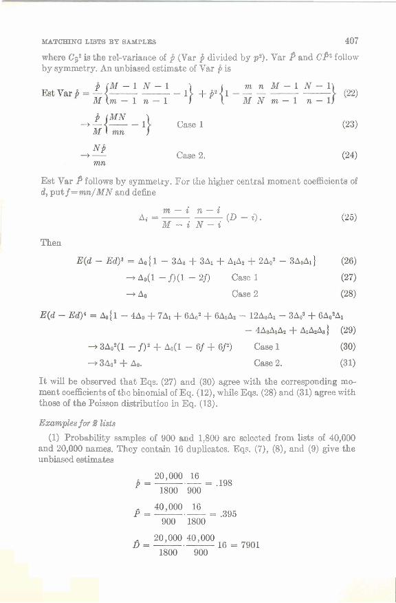
where CG2 is the rel-variance of j3 (Var $ divided by p2). Var p and C'p2 follow by symmetry. An unbiased estimate of Var j3 is

Case 1

Case 2.

Est Var 9 follows by symmetry. For the higher central moment coefficients of d, put f =mn/MN and d e h e

m - i n - i &=-- (D - i).

M - i N - i

Then

Case 1

Case 2

Case 1

4 3A04 + AO. Case 2. (31)

It will be observed that Eqs. (27) and (30) agree with the corresponding mo- ment coefficients of the binomial of Eq. (12), while Eqs. (28) and (31) agree with those of the Poisson distribution in Eq. (13).

Examples for d lists

(1) Probability samples of 900 and 1,800 are selected from lists of 40,000 and 20,000 names. They contain 16 duplicates. Eqs. (7), (8), and (9) give the unbiased estimates

408

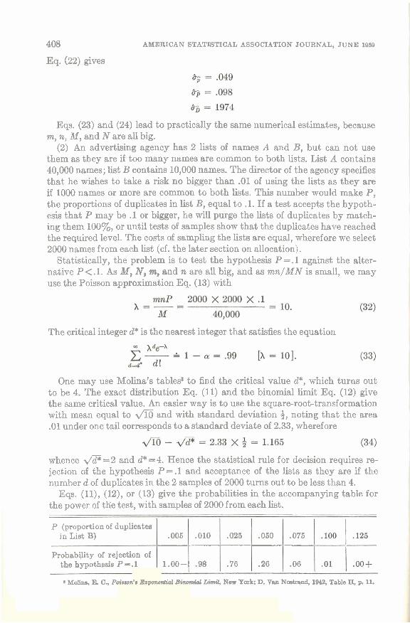
Eq. (22) gives

AMERICAN STATISTICAL ASSOCIATION JOURNAL, JUNE 1959

Eqs. (23) and (24) lead to practically the same numerical e~timat~es, because m, n, M , and N are all big.

(2) An advertising agency has 2 lists of names A and B, but can not use them as they are if too many names are common to both lists. List A contains 40,000 names; list B contains 10,000 names. The director of the agency specifies that he wishes to take a risk no bigger than .O1 of using the lists as they are if 1000 names or more are common to both lists. This number would make P, the proportions of duplicates in list B, equal to .l. If a test accepts the hypoth- esis that P may be .1 or bigger, he will purge the lists of duplicates by match- ing them loo%, or until tests of samples show that the duplicates have reached the required level. The costs of sampling the lists are equal, wherefore we select 2000 names from each list (cf. the later section on allocation).

Statistically, the problem is to test the hypothesis P =. 1 against the alter- native P< .l. As M, N, m, and n are all big, and as mn/MN is small, we may use the Poisson approximation Eq. (13) with

The critical integer d* is the nearest integer that satisfies the equation

One may use Molina's tablesa to find the critical value d*, which turns out to be 4. The exact distribution Eq. (11) and the binomial limit Eq. (12) give the same critical value. An easier way is to use the square-root-transformation with mean equal to di6 and with standard deviation 3, noting that the area -01 under one tail corresponds to a standard deviate of 2.33, wherefore

whence 2 / 3 = 2 and d* =4. Hence the statistical rule for decision requires re- jection of the hypothesis P = .l and acceptance of the lists as they are if the number d of duplicates in the 2 samples of 2000 turns out to be less than 4.

Eqs. ( l l ) , (12), or (13) give the probabilities in the accompanying table for the power of tlie test, with samples of 2000 from each list.

a M o l i ~ , E. C., Poism'a ExponenW Binomial Limit, New York: D. Van Nostrand, 1942, Table 11, p. 11.

P (proportion of duplicates in List B)

Probability of rejection of the hypothesis P 1.1

.006

1.00- .98

.025 -----

.76

.010 .050

.26

.075

.06

MATCHENG LIBm BY SAMPLES

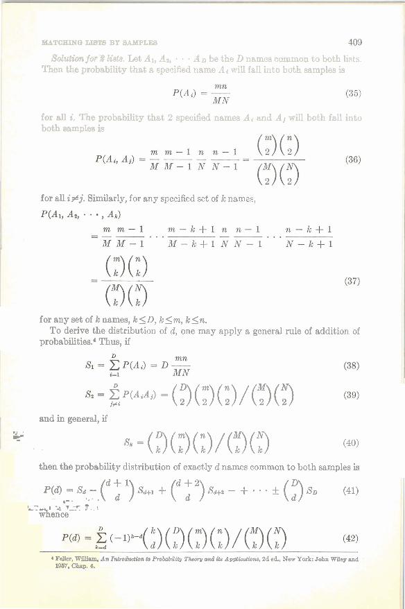
Solution for $3 lists. Let AI, Az, . . . AB be the D names cammon to both lists. Then the probability that a specified name Ai will fall into both samples is

for all i. The probability that 2 specified names Ai and A, will bath fall into both s a m ~ h is

for all i#j. Similarly, for any specified set of k names,

for any set of knames, k s D , k l m , k l n . To derive the distribution of d, one may apply a general rule of addition of

probabilities.' Thus, if

M N = $ p ( ~ i ~ j ) = (3 ( y) (i) / ( 2 ) ( 2 )

and in general, if

3 . . sk = (3(3(2)/(3(3 (40)

I then the probability distribution of exactly d names common to both samples is

d + l d f 2 ~ ( a = . - ( *-, - a 7 . , ) s d H + ( ) s ~ ~ - + . . - & ( f i ? ~ ~ (41)

I -& 7-- f .. L

I '-3 w ence

4 Feller, W i . An Introdudion to Probability T h r y and ita Applications, 2d ed., New York: John Wiey and 1967. Chap. 4.

AMERICAN STATISTICAL ASSOCIATION JOURNAL, JUNE 1969

- - \ d l D - M - D N -

(30 ~ ( k - > ( m - k ) ( n - t )

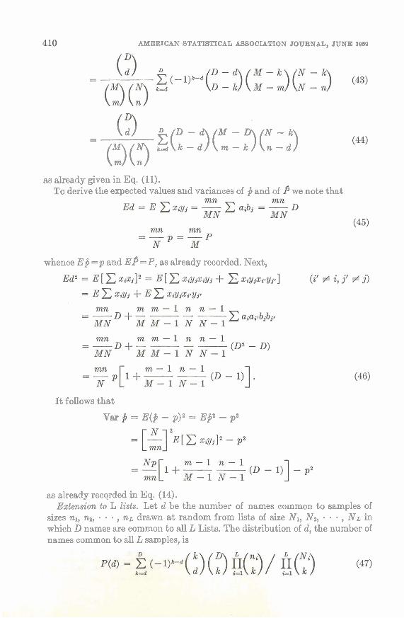
as already given in Eq. (11) . To derive the expected values and variances of j and of we note that

whence Ep = p and EP= P , as already recorded. Next,

It follows that

Var = E(j3 - P ) ~ = E j 2 - p1

as already recorded in Eq. (14) . Extension to L lists. Let d be the number of names common to samples of

sizes nl, n2, - . . , n~ drawn a t random from lists of size N,, N2, . . - , N L ~LI which D names are common to all L Lists. The distribution of d , the number of names common to all L samples, is

MATCHING LISTS BY SAMPLES '

and asymptotic results analogous to Eq. (12) and Eq. (13) include

Case 1

Case 2

where

Put now

X = Dj.

wherein i runs here and hereafter from 1 to L. Then fi is an unbiased estimate of D, and

Case 1

Case 2.

An unbiased estimate of this variance is

Case 1

Case 2.

Optimum sample-sizes. For matching 2 samples let the costs be: CI to draw a name from List 1, and to write it down or to prepare a card

therefor, in preparation to compare it with the sample from List 2. cl includes also a proper share of the cost of sorting the cards of the sample to put them in alphabetic order.

cn the same for List 2. c8 to compare a name in one sample with a name in the other sample, and

to record the comparison as 0 or 1.

412 AMERICAN STATISTICAL ASSOCIATION JOURNAL, JUNE 19M)

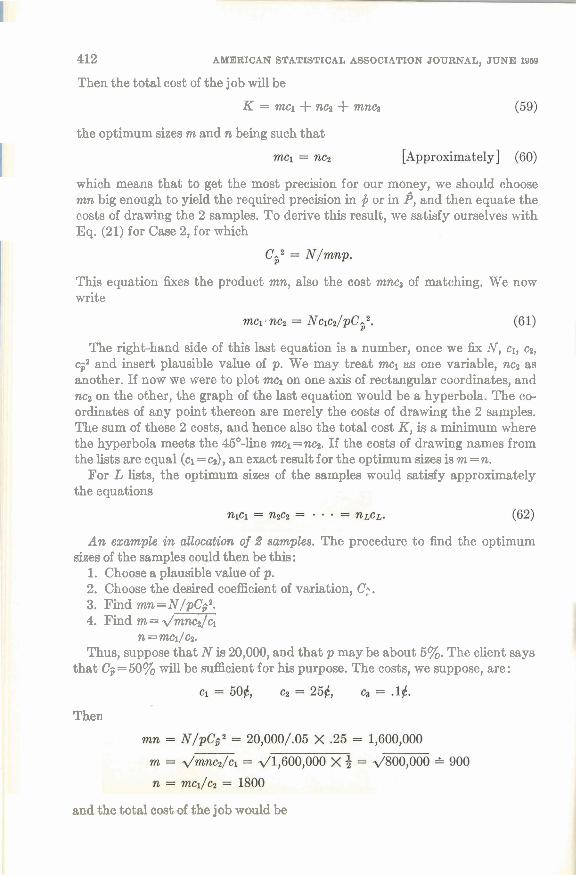
Then the total cost of the job will be

K = m c ~ + n c ~ + mnq

the optimum sizes m and n being such that

which means that to get the most precision for our money, we should choose mn big enough to yield the required precision in # or in P, and then equate the costs of drawing the 2 samples. To derive this result, we satisfy ourselves with Eq. (21) for Case 2, for which

This equation fixes the product mn, also the cost mncg of matching. We now write

The right-hand side of this last equation is a number, once we h N, cl, c2, 5% and insert plausible value of p. We may treat mcl as one variable, ncz as another. If now we were to plot me1 on one axis of rectangular coordinates, and nc2 on the other, the graph of the last equation would be a hyperbola. The co- ordinates of any point thereon are merely the costs of drawing the 2 samples. The sum of these 2 costs, and hence also the total cost K, is a minimum where the hyperbola meets the 45'-he mcr=nco . If the costs of drawing names from the lists are equal (cl = c3, an exact result for the optimum sizes is m = n.

For L lists, the optimum sines of the samples would satisfy approximately the equations

An example in allocation of 3 samples. The procedure to find the optimum s h s of the samples could then be this:

1. Choose a plausible value of p. 2. Choose the desired coefficient of variation, C:. 3. Find m n = N / P C ~ ~ . 4. Find m = dmn%/cl

n = ml/ct. Thus, suppose that N is 20,000, and that p may be about 5%. The client says

that C5=50% will be sufficient for his purpose. The costs, we suppose, are:

Then

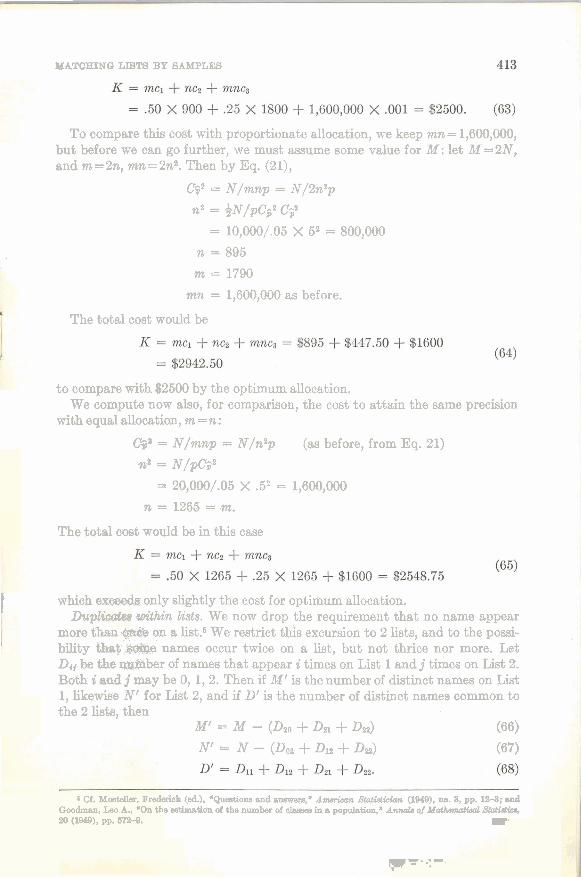
and the total cost of the job would be

~ ~ H I N Q LISTS BY SAMPLES

To compare this cost with proportionate allocation, we keep mn = 1,600,000, but before we can go further, we must assume some value for M: let M=2N, and m = 2n, mn = 2ne. Then by Eq. (2 I),

C;;" N/mnp = N/2n2p

n2 = *N/pCG2 C2 = 10,000/.05 X 52 = 800,000

n = 895 1 -

m = 1790

mn = 1,600,000 as before.

The total cost would be

to compare with $2500 by the optimum allocation. We compute now also, for comparison, the cost to attain the same precision

with equal allocation, m = n :

Cs3 = N/mnp = N/n2p (as before, from Eq. 21)

%* = N/pClij2

= 20,000/.05 X .!j2 = 1,600,000

n = 1265 = m.

The tots1 cost would be in this case

I which ex& only slightly the cost for optimum allocation. Du Whin lists. We now drop the requirement that no name appear

more than$@& on a list.6 We restrict this excursion to 2 lists, and to the possi- bility th&$ &a@e names occur twice on a list, but not thrice nor more. Let Dti be the ra&ber of names that appear i times on List 1 and j times on List 2. Both i md j may be O,1,2. Then if M' is the number of distinct names on List 1, likewise N' for List 2, and if D' is the number of distinct names common to the 2 lists, then

M' = M - (D2o + Dei + D d (66)

N' = N - (Doe + Du + Dza) (67)

6 Cf. Marteller, Frederi~k (ed), "Qu@iona and ~ ~ ~ w e r s , ' American 8 W i c i o n (IMQ), ne. a, pp. 12-a; and Goodman, Leo A., 'On the eathation of the number of a k w a in a p~pulstian,~ A n d of M d h t n & d &tWm, ZO (lW), pp. 872-0.

rlnr*.:--

AMERICAN STATISTICAL ASSOCIATION JOURNAL, JUNE 1959

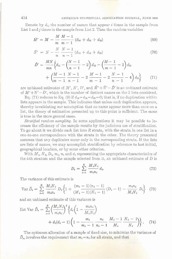
Denote by dij the number of names that appear i times in the sample from List 1 and j times in the sample from List 2. Then the random variables

N N - 1 P = N - - - (dot + dl2 -I- dtt) n n - 1

are unbiased estimates of M', N', D', and at+20'-D is an unbiased estimate of Mf+N'-D', which is the number of distinct names on the 2 lists combined.

Eq. (71) reduces to Eq. (9) if dl2 = dzt = dtt = 0; that is, if no duplication within lists appears in the sample. This indicates that unless such duplication appears, thereby invalidating our assumption that no name appear more than once on a list, the theory of estimation presented up to this point is sufficient. The same is true in the more general cases.

Stratijied random sampling. In some applications it may be possible to in- crease the efficiency of the sample results by the judicious use of stratification. To go about it we divide each list into R strata, with the strata in one list in a one-to-one correspondence with the strata in the other. The theory presented assumes that any duplicates occur only in the corresponding strata. If the lists are Lists of names, we may accomplish stratification by reference to last initial, geographical location, or by some other criterion.

With Mc Nc, Di, mi, ni and di representing the appropriate characteristics of the i-th stratum and the sample selected from it, an unbiased estimate of D is

The variance of this estimate is

M a c (mi - l)(ni - 1) varb . = c - ~ , { l + (0, - 1) - -

bl m,ni (Mi - l)(Ni - 1) msi D,) (73)

MiNi

and an unbiased estimate of this variance is

( (mi) Est Var b. = % - di 1--

i-1 msni MiNi

The optimum allocation of a sample of fixed size, to minimize the variance of B,, involves the requirement that

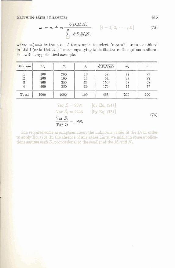
[i - 1,2, . . , R ]

i-1

Var $ = 2321 [by Eq. (21)] Var B, = 2223 [by Eq. (73)]

One requires some as~umption about the unknown values of the D1 in order to apply Eq. (75). In the absence of any other hints, we might in some applicrt- tions assume each D+ proportional to the smaller af the Mi and Nr.