on the viscous burgers equation in unbounded domain filewhole real line r. this becomes possible due...
TRANSCRIPT

Electronic Journal of Qualitative Theory of Differential Equations
2010, No. 18, 1-23; http://www.math.u-szeged.hu/ejqtde/
On the viscous Burgers equation in unbounded domain
j. lımaco 1, h. r. clark 1, 2 & l. a. medeiros 3
Abstract
In this paper we investigate the existence and uniqueness of global solutions, and
a rate stability for the energy related with a Cauchy problem to the viscous Burgers
equation in unbounded domain R× (0,∞). Some aspects associated with a Cauchy
problem are presented in order to employ the approximations of Faedo-Galerkin in
whole real line R. This becomes possible due to the introduction of weight Sobolev
spaces which allow us to use arguments of compactness in the Sobolev spaces.
Key words: Unbounded domain, global solvability, uniqueness, a rate decay estimate
for the energy.
AMS subject classifications codes: 35B40, 35K15, 35K55, 35R35.
1 Introduction and Formulation of the Problem
We are concerned with the existence of global solutions – precisely, global weak
solutions, global strong solutions and regularity of the strong solutions –, uniqueness
of the solutions and the asymptotic stability of the energy for the nonlinear Cauchy
problem related to the classic viscous Burgers equation
ut + uux − uxx = 0
established in R × (0, T ), for an arbitrary T > 0. More precisely, we consider the real
valued function u = u(x, t) defined for all (x, t) ∈ R× (0, T ) which is the solution of the
Cauchy problem{ut + uux − uxx = 0 in R × (0, T ),
u(x, 0) = u0(x) in R.(1.1)
1Universidade Federal Fluminense, IM, RJ, Brasil2Corresponding author: [email protected] Federal do Rio de Janeiro, IM, RJ, Brasil, [email protected]
EJQTDE, 2010 No. 18, p. 1

The Burgers equation has a long history. We briefly sketch this history by citing
one of the pioneer work by Bateman [2] about an approximation of the flux of fluids.
Later, Burgers published the works [5] and [6] which are also about flux of fluids or
turbulence. In the classic fashion the Burgers equation has been studied by several
authors, mainly in the last century, and excellent papers and books can be found in
the literature specialized in PDE. One can cite, for instance, Courant & Friedrichs [8],
Courant & Hilbert [9], Hopf [10], Lax [13] and Stoker [17].
Today, the equation (1.1)1 ((1.1)1 refers to the first equation in (1.1)) is known as
viscous Burgers equations and perhaps it is the simplest nonlinear equation associating
the nonlinear propagation of waves with the effect of the heat conduction.
The existence of global solutions for the Cauchy problem (1.1) will be obtained
employing the Faedo-Galerkin and Compactness methods. The Faedo-Galerkin method
is probably one of the most effective methods to establish existence of solutions for non-
linear evolution problems in domains whose spatial variable x lives in bounded sets. To
spatial unbounded sets, there exist few results about existence of solutions established
by the referred method. Thus, as the non-linear problem (1.1) is defined in R, in order
to reach our goal through this method we will also need to use compactness’ argument,
as in Aubin [1] or Lions [15]. In order to apply the Compactness method we employ
a suitable theory on weight Sobolev spaces to be set as follows. In fact, in the sequel
Hm(R) represents the Sobolev space of order m in R, with m ∈ N. The space L2(R)
is the Lebesgue space of the classes of functions u : R → R with square integrable on
R. Assuming that X is a Banach space, T is a positive real number or T = +∞ and
1 ≤ p ≤ ∞, we will denote by Lp(0, T ;X) the Banach space of all measurable mapping
u :]0, T [−→ X, such that t 7→ ‖u(t)‖X belongs to Lp(0, T ). For more details on the
functional spaces above cited the reader can consult, for instance, the references [3] and
[15]. In this work we will also use the following weight vectorial spaces
L2(K) ={φ ∈ L2(R);
∫
R
|φ(y)|2RK(y)dy <∞},
Hm(K) ={φ ∈ Hm(R); Diφ ∈ L2(K)
}with i = 1, 2, . . . ,m, m ∈ N,
where K is a weight function given for
K(y) = exp{y2/4}, y ∈ R. (1.2)
EJQTDE, 2010 No. 18, p. 2

The inner product and norm of L2(K) and Hm(K) are defined by
(φ,ψ) =
∫
R
φ(y)ψ(y)K(y)dy, |φ|2 =
∫
R
|φ(y)|2RK(y)dy,
((φ,ψ))m =m∑
i=1
∫
R
Diφ(y)Diψ(y)K(y)dy, ‖φ‖2m =
m∑
i=1
∣∣Diφ∣∣2 ,
respectively. The vector spaces L2(K) and Hm(K) are Hilbert spaces with the above
inner products. By D(R) it denotes the class of C∞ functions in R with compact
support and convergence in the Laurent Schwartz sense, see [16].
We will also use the functional structure of the spaces Lp(0, T ;H) with 1 ≤ p ≤ ∞,
where H is one of the spaces: L2(K) or Hm(K).
Some properties of the spaces L2(K) and Hm(K) as the compactness of the inclu-
sion Hm(K) → L2(K) and Poincare inequality with the weight (1.2) has been proven
in Escobedo-Kavian [11]. Results on compactness of space of spherically symmetric
functions that vanishes at infinity were proven by Strauss [18]. In this direction one
can see some results in Kurtz [12].
The method used to prove the existence of solutions for the Cauchy problem (1.1)
is to transform it to another equivalent one proposed in the suitable functional spaces
by using a change of variables defined by
z(y, s) = (t+ 1)1/2u(x, t) where y =x
(t+ 1)1/2and s = ln(t+ 1). (1.3)
The changing of variable (1.3) defines a diffeomorphism σ : Rx × (0, T ) → Ry × (0, S)
with σ(x, t) = (y, s) and S = ln(T + 1). From (1.3) we have t = es − 1 and x = es/2y.
Therefore,
z(y, s) = es/2u(es/2y, es − 1) and u(x, t) = (t+ 1)−1/2z(x/(t+ 1)1/2, ln(t+ 1)
).
Differentiating u with respect to t, it yields
ut =−1
2(t+ 1)−3/2z + (t+ 1)−1/2
(∂z∂y
∂y
∂t+∂z
∂s
∂s
∂t
)
= (t+ 1)−3/2(− z
2− yzy
2+ zs
)
= e−3s/2(− z
2− yzy
2+ zs
).
EJQTDE, 2010 No. 18, p. 3

Differentiating u with respect to x, it yields
ux = (t+ 1)−1/2 ∂z
∂y
∂y
∂x= (t+ 1)−1/2 ∂z
∂y
1
(t+ 1)1/2= (t+ 1)−1zy = e−szy.
Differentiating again with respect to x, it yields
uxx = (t+ 1)−1 ∂2z
∂y2
∂y
∂x= (t+ 1)−3/2zyy = e−3s/2zyy.
Inserting the three last identities in (1.1)1, we obtain
zs − zyy −yzy2
− z
2+ zzy = 0 in R × (0, S). (1.4)
Moreover, for t = 0, we have by definition of y that x = y. Thus the initial data
becomes
u0(x) = u(x, 0) = z(y, 0) = z0(y). (1.5)
For use later and a better understanding we will modify the equation (1.4) as follows:
one defines the operator L : H2(K) −→ R by φ 7−→ Lφ = −φyy − yφy
2 , which satisfies:
Lφ = − 1
K(Kφy)y and (Lφ,ψ) = (φy, ψy) = ((φ,ψ))2 (1.6)
for all φ ∈ H2(K) and ψ ∈ H1(K). Therefore, from (1.4), (1.5) and (1.6)1 the Cauchy
problem (1.1) is equivalent by σ to
zs + Lz − z
2+ zzy = 0 in R × (0, S),
z(y, 0) = u0(y) in R.(1.7)
The purpose of this work is: in Section 2, we investigate the existence of global weak
solutions of (1.1), its uniqueness and as well as analysis of the decay of these solutions.
In Section 3 we establish the same properties of Section 2 for the strong solutions. In
Section 4, we study the regularity of the strong solutions.
2 Weak Solution
Setting the initial data u0 ∈ L2(K) we are able to show that the Cauchy problem
(1.1) has a unique global weak solution u = u(x, t) defined in R×(0,∞) with real values
and the energy associated with this solution is asymptotically stable.
The concept of the solutions for (1.1) is established in the following sense
EJQTDE, 2010 No. 18, p. 4

Definition 2.1. A global weak solution for the Cauchy problem (1.1) is a real valued
function u = u(x, t) defined in R × (0,∞) such that
u ∈ L2loc(0,∞;H1(R)), ut ∈ L2
loc
(0,∞; [H1(R)]′
),
the function u satisfies the identity integral
−∫ T
0
∫
R
[uv]ϕtdxdt +
∫ T
0
∫
R
[uuxv]ϕdxdt +
∫ T
0
∫
R
[uxvx]ϕdxdt = 0, (2.1)
for all v ∈ H1(R) and for all ϕ ∈ D(0, T ). Moreover, u satisfies the initial condition
u(x, 0) = u0(x) for all x ∈ R.
The existence of solution of (1.1) in the precedent sense is guaranteed by the fol-
lowing theorem
Theorem 2.1. Suppose u0 ∈ L2(K), then there exists a unique global solution u of
(1.1) in the sense of Definition 2.1. Moreover, energy E(t) = 12 |u(t)|2 associated with
this solution satisfies
E(t) ≤ E(0)(t + 1)−3/4. (2.2)
The following proposition, whose proof has have been done in Escobedo & Kavian
[11], will be useful throughout this paper.
Proposition 2.1. One has the results
(1)
∫
R
|y|2|v(y)|2RKdy ≤ 16
∫
R
|vy(y)|2RKdy for all v ∈ H1(K);
(2) The immersion H1(K) → L(K) is compact;
(3) L : H1(K) −→ [H1(K)]′ is an isomorphism;
(4) The eigenvalues of L are positive real numbers λj = j/2 for j = 1, 2 . . . , and
the related space with λj is N(L− λjI) =[Djω1
]with
ω1(y) =1
(4π)1/4[K(y)]−1 =
1
(4π)1/4exp{−y2/4}.
(5) Finally, one has the Poincare inequality |v| ≤√
2 |vy| for v ∈ H1(K)
As the two Cauchy problems (1.1) and (1.7) are equivalent the Definition 2.1 and
Theorem 2.1 are also equivalent to Definition 2.2 and Theorem 2.2.
EJQTDE, 2010 No. 18, p. 5

Definition 2.2. A global weak solution for the Cauchy problem (1.7) is a real valued
function z = z(y, s) defined in R × (0,∞) such that
z ∈ L2loc(0,∞;H1(K)), zs ∈ L2
loc
(0,∞; [H1(K)]′
),
the function z satisfies the identity integral
−∫ S
0
∫
R
[zv]ϕsKdyds+
∫ S
0
∫
R
[zzyv]ϕKdyds+
∫ S
0
∫
R
[zyvy]ϕKdyds−1
2
∫ S
0
∫
R
[zv]ϕKdyds = 0, (2.3)
for all v ∈ H1(K) and for all ϕ ∈ D(0, S). Moreover, z satisfies the initial condition
z(y, 0) = z0(y) for all y ∈ R.
The existence of solutions for system (1.7) will be shown by means of Faedo-Galerkin
method. In fact, as L2(K) is a separable Hilbert space there exists a orthogonal hilber-
tian basis (ωj)j∈N of L2(K). Moreover, since H1(K) → L2(K) is compactly imbedding
there exist ωj solutions of the spectral problem associated with the operator L in H1(K).
This means that
(Lωj, v) = λj(ωj , v) for all v ∈ H1(K) and j ∈ N. (2.4)
Fixed the first eigenfunction ω1 of L we set {ω1}⊥ ={v ∈ L2(K); (ω1, v) = 0
}.
In these conditions one defines VN as the subspace of L2(K) spanned by the N−eigenfunction ω1, ω2, . . . , ωN of (ωj)j∈N, being ωj with j ∈ N defined by (2.4).
Now, we are ready to state the following result.
Theorem 2.2. Suppose z0 ∈ L2(K) ∩ {ω1}⊥, then there exists a unique solution
z of (1.7) in the sense of Definition 2.2, provided |z0| < 14√
3C1
holds, where C1 is
a positive real constant defined below in the Proposition 2.2-item (b). Moreover, the
energy E(s) = 12 |z(s)|2 satisfies
E(s) ≤ E(0) exp [−s/4] . (2.5)
Since Theorems 2.1 and 2.2 are equivalent, it suffices to prove the Theorem 2.2.
Before this, we first introduce the following property, which will be useful later:
EJQTDE, 2010 No. 18, p. 6
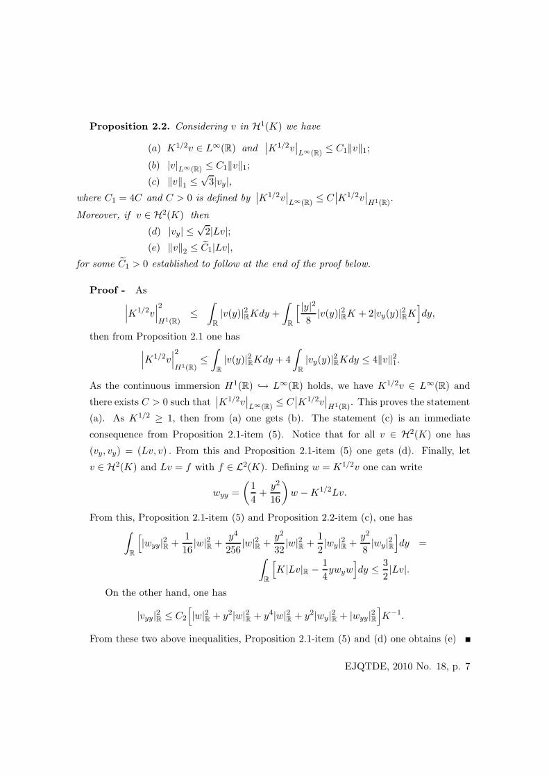
Proposition 2.2. Considering v in H1(K) we have
(a) K1/2v ∈ L∞(R) and∣∣K1/2v
∣∣L∞(R)
≤ C1‖v‖1;
(b) |v|L∞(R) ≤ C1‖v‖1;
(c) ‖v‖1 ≤√
3|vy|,where C1 = 4C and C > 0 is defined by
∣∣K1/2v∣∣L∞(R)
≤ C∣∣K1/2v
∣∣H1(R)
.
Moreover, if v ∈ H2(K) then
(d) |vy| ≤√
2|Lv|;(e) ‖v‖2 ≤ C1|Lv|,
for some C1 > 0 established to follow at the end of the proof below.
Proof - As∣∣∣K1/2v
∣∣∣2
H1(R)≤
∫
R
|v(y)|2RKdy +
∫
R
[ |y|28
|v(y)|2RK + 2|vy(y)|2RK]dy,
then from Proposition 2.1 one has∣∣∣K1/2v
∣∣∣2
H1(R)≤∫
R
|v(y)|2RKdy + 4
∫
R
|vy(y)|2RKdy ≤ 4‖v‖21.
As the continuous immersion H1(R) → L∞(R) holds, we have K1/2v ∈ L∞(R) and
there exists C > 0 such that∣∣K1/2v
∣∣L∞(R)
≤ C∣∣K1/2v
∣∣H1(R)
. This proves the statement
(a). As K1/2 ≥ 1, then from (a) one gets (b). The statement (c) is an immediate
consequence from Proposition 2.1-item (5). Notice that for all v ∈ H2(K) one has
(vy, vy) = (Lv, v) . From this and Proposition 2.1-item (5) one gets (d). Finally, let
v ∈ H2(K) and Lv = f with f ∈ L2(K). Defining w = K1/2v one can write
wyy =
(1
4+y2
16
)w −K1/2Lv.
From this, Proposition 2.1-item (5) and Proposition 2.2-item (c), one has∫
R
[|wyy|2R +
1
16|w|2R +
y4
256|w|2R +
y2
32|w|2R +
1
2|wy|2R +
y2
8|wy|2R
]dy =
∫
R
[K|Lv|R − 1
4ywyw
]dy ≤ 3
2|Lv|.
On the other hand, one has
|vyy|2R ≤ C2
[|w|2R + y2|w|2R + y4|w|2R + y2|wy|2R + |wyy|2R
]K−1.
From these two above inequalities, Proposition 2.1-item (5) and (d) one obtains (e)
EJQTDE, 2010 No. 18, p. 7

Proof of Theorem 2.2 - We will employ the Faedo-Galerking approximate method
to prove the existence of solutions. In fact, the approximate system is obtained from
(2.4) and this consists in finding zN (s, y) =N∑
i=1giN (s)ωi(y) ∈ VN , the solution of the
system of ordinary differential equations
(zNs (s), ω
)+(LzN (s), ω
)− 1/2
(zN (s), ω
)+(zN (s)zN
y (s), ω)
= 0,
zN (0) = zN0 =
N∑
j=1
(z0, ωj)ωj ,(2.6)
for all ω belong to VN . The System (2.6) has local solution zN in 0 ≤ s < sN , see for
instance, Coddington-Levinson [7]. The estimates to be proven later allow us to extend
the solutions zN to whole interval [0, S[ for all S > 0 and to obtain subsequences that
converge, in convenient spaces, to the solution of (1.7) in the sense of Definition 2.2.
Estimate 1. Setting ω = zN (s) ∈ VN in (2.6)1, it yields
1
2
d
ds
∣∣zN (s)∣∣2 +
∣∣zNy (s)
∣∣2 − 1
2
∣∣zN (s)∣∣2 +
∫
R
zN (s)zNy (s)zN (s)Kdy = 0.
The integral above is upper bounded. In fact, by using Holder inequality, Proposition
2.1-item (5) and Proposition 2.2-item (b) we can write∣∣∣∫
R
zN (s)zNy (s)LzN (s)Kdy
∣∣∣R
≤√
3C1
∣∣zNy (s)
∣∣2 ∣∣zN (s)∣∣ .
From this and from precedent identity we get
1
2
d
ds
∣∣zN (s)∣∣2 +
1
2
∣∣zNy (s)
∣∣2 +1
2
( ∣∣zNy (s)
∣∣2 −∣∣zN (s)
∣∣2)≤
√3C1
∣∣zNy (s)
∣∣2 ∣∣zN (s)∣∣ . (2.7)
By using (1.6)2, the fact that basis (ωj) is orthonormal and (2.4) we have
∣∣zNy (s)
∣∣2 =
N∑
j=1
(gjN (s))2 λj and |zN (s)|2 =
N∑
j=1
(gjN (s))2 .
By using these two identities we are able to prove that
1
2
(|zN
y (s)|2 − |zN (s)|2)≥ 0 for all N ∈ N. (2.8)
In fact, note that
1
2
(|zN
y (s)|2 − |zN (s)|2)
=1
2(g1N (s))2 (λ1 − 1) +
1
2
N∑
j=2
(gjN (s))2 (λj − 1) .
EJQTDE, 2010 No. 18, p. 8

Next one can prove that
g1N (s) = 0 and
N∑
j=2
(gjN (s))2 (λj − 1) ≥ 0 for all s and N. (2.9)
From Proposition 2.1-item (4) the second statement in (2.9) is obvious. Therefore, it
suffices to prove that g1N (s) = 0 for all s and N. In fact, first, note that
g1N (s) =( N∑
j=1
gjN (s)ωj , ω1
)= (zN (s), ω1) .
Thus, we will show that (zN (s), ω1) = 0. Setting ω = ω1 ∈ VN in (2.6)1, it yields
(zNs (s), ω1
)+(LzN (s), ω1
)− 1
2
(zN (s), ω1
)+(zN (s)zN
y (s), ω1
)= 0. (2.10)
By using (2.4) and Proposition 2.1-item (4) one can writes
(LzN (s), ω1
)=
1
2
(zN (s), ω1
).
The non-linear term of (2.10) is null, because
(zN (s)zN
y (s), ω1
)=
1
2
1
(4π)1/4
∫
R
[(zN (s)
)2]
ydy.
we have used above Proposition 2.1-item (4), that is,
ω1(y) =1
(4π)1/4exp{−y2/4}.
From this, as ωj ∈ H1(K) then(zN)2
and(zNy
)2belong to L1(R) and consequently
lim|y|−→∞
zN (y, t) = 0. Thus,(zN (s)zN
y (s), ω1
)= 0 for all N and s. Taking into account
these facts in (2.10), it yields(zNs (s), ω1
)= 0. Thus, by using (2.6)2 and hypothesis
on z0 we get(zN (s), ω1
)=(zN (0), ω1
)= 0. Therefore, this completes the proof of
statement of (2.9)
Since (2.8) is true, the inequality (2.7) is reduced to
1
2
d
ds
∣∣zN (s)∣∣2 +
1
4
∣∣zNy (s)
∣∣2 +∣∣zN
y (s)∣∣2(1
4−
√3C1
∣∣zN (s)∣∣)≤ 0. (2.11)
Next, we will prove that
|zN (s)| < 1
4√
3C1
for all s ≥ 0. (2.12)
EJQTDE, 2010 No. 18, p. 9

In fact, suppose it is not true. Then there exists s∗ such that
|zN (s)| < 1
4√
3C1
for all 0 ≤ s < s∗ and |zN (s∗)| =1
4√
3C1
.
Integrating (2.11) from 0 to s∗, it yields
1
2|zN (s∗)|2 +
1
4
∫ s∗
0|zN
y (s)|2ds +
∫ s∗
0|zN
y (s)|2(1
4−
√3C1|zN (s)|
)ds ≤ 1
2|z0|2.
From hypothesis on z0 we have
|zN (s∗)| < 1/4√
3C1.
This contradicts∣∣zN (s∗)
∣∣ = 1/4√
3C1. Thus, (2.12) it is true. Therefore, integrating
(2.11) from 0 to s and by using (2.4) and (2.6)2, it yields
|zN (s)|2 +1
2
∫ s
0|zN
y (τ)|2dτ ≤ |z0|2 ≤ 1
4√
3C1
. (2.13)
Estimate 2. In this estimate we will use the projection operator
PN : L2(K) −→ VN defined by v 7−→ PN (v) =
N∑
i=1
(v, ωi)ωi.
Thus, from (2.6)1 we have
N∑
i=1
(zNs , ωi)ωi +
N∑
i=1
(LzN , ωi)ωi −1
2
N∑
i=1
(zN , ωi)ωi +
N∑
i=1
(zN (s)zNy (s), ωi)ωi = 0.
From this and definition of PN one can write
PN
(zNs
)+ PN
(LzN
)− 1
2PN
(zN)
+ PN
(zN (s)zN
y (s))
= 0.
As PNVN ⊂ VN and zN ; zNs ; LzN ∈ VN , then
zNs = −LzN +
1
2zN − PN
(zN (s)zN
y (s)). (2.14)
EJQTDE, 2010 No. 18, p. 10

The identity (2.14) is verified in the L∞(0, S;
[H1(K)
]′)sense. In fact, analyzing each
term on the right-hand side of (2.14) we prove this statement as one can see:
|LzN (s)|[H1(K)]′ = supv∈H1(K)||v||1≤1
∣∣∣(zNy (s), vy
)L2(K)
∣∣∣R
≤∣∣zN
y (s)∣∣ . (2.15)
|zN (s)|[H1(K)]′ = supv∈H1(K)||v||1≤1
∣∣∣(zN (s), v
)L2(K)
∣∣∣R
≤∣∣zN (s)
∣∣ . (2.16)
∣∣PN
(zN (s)zN
y (s))∣∣
[H1(K)]′≤ C1 sup
v∈H1(K)||v||1≤1
∣∣zN (s)∣∣ ∣∣zN
y (s)∣∣ ‖(PNv)‖H1(K)
≤∣∣zN (s)
∣∣ ∣∣zNy (s)
∣∣ . (2.17)
As the proof of the three identities (2.15), (2.16) and (2.17) are similar, we will just
make the last one. In fact,
∣∣PN
(zN (s)zN
y (s))∣∣
[H1(K)]′= sup
v∈H1(K)||v||≤1
∣∣∣⟨PN
(zN (s)zN
y (s)), v⟩[H1(K)]′×H1(K)
∣∣∣R
= supv∈H1(K)||v||≤1
∣∣∣(PN
(zN (s)zN
y (s)), v)L2(K)
∣∣∣R
= supv∈H1(K)||v||≤1
∣∣∣(zN (s)zN
y (s), PNv)L2(K)
∣∣∣R
≤ C1 supv∈H1(K)||v||≤1
∣∣zN (s)∣∣ ∣∣zN
y (s)∣∣ ‖(PNv)‖H1(K) .
On the other hand,
‖(PNv)‖2H1(K) =
∥∥∥N∑
i=1
(v, ωi)ωi
∥∥∥2
=
N∑
i=1
(v, ωi)2(ωiy, ωiy)
=
N∑
i=1
(v, ωi)2(Lωi, ωi) =
N∑
i=1
(v, ωi)2λi
=
N∑
i=1
(v,Lωi√λi
)2
=
N∑
i=1
(vy,
ωiy√λi
)2
≤∞∑
i=1
(vy,
ωiy√λi
)2
= ‖v‖2H1(K) ≤ 1.
EJQTDE, 2010 No. 18, p. 11

Inserting this inequality in the precedent one we get (2.17). By using (2.15)-(2.17) in
(2.14), we get
|zNs (s)|2
[H1(K)]′≤
[1
2|zN (s)| +
(1 + C1|zN (s)|
)|zN
y (s)|]2
≤[(√
2
2+ 1 +C1|zN (s)|
)|zN
y (s)|]2
≤[(√
2
2+ 1 +
C1
2√√
3C1
)|zN
y (s)|]2
,
where we have used in the two last step the Poincare inequality and Estimate (2.13).
Integrating this inequality from 0 to S and again using Estimate (2.13), we obtain∫ S
0|zN
s (s)|2[H1(K)]′
ds ≤ C, (2.18)
where
C =
(√2
2+ 1 +
C1
2√√
3C1
)21
2√
3C1
.
The limit in the approximate problem (2.6): By Estimates 1 and 2, more pre-
cisely, from (2.13) and (2.18) we can extract subsequences of (zN ), which one will
denote by (zN ), and a function z : R × (0, S) → R satisfying∣∣∣∣∣∣∣∣
zN ⇀ z weak star in L∞ (0, S;L2(K)),
zN ⇀ z weak in L2(0, S;H1(K)
),
zNs ⇀ zs weak in L2
(0, S;
[H1(K)
]′).
(2.19)
From these convergence we are able to pass to the limits in the linear terms of (2.6). The
nonlinear term needs careful analysis. In fact, from (2.19)1, 3 and Aubin’s compactness
result, see Aubin [1], Browder [4], Lions [15] or Lions [14], we can extract a subsequences
of (zN ), which one will denote by (zN ), such that
zN → z strongly in L2(0, S;L2(K)). (2.20)
On the other hand, for all φ(x, s) = v(x)θ(s) with v ∈ H1(K) and θ ∈ D(0, S) we have∫ S
0
(zN (s)zN
y (s), φ(s))ds =
∫ S
0
(zNy , z
Nφ)ds (2.21)
=
∫ S
0
(zNy ,[zN − z
]φ)ds+
∫ S
0
(zNy , zφ
)ds.
EJQTDE, 2010 No. 18, p. 12

Next, we will show that the last two integrals on the right-hand side of (2.21) converge.
In fact, the first one can be upper bounded as follows
∣∣∣∫ S
0
(zNy ,[zN − z
]φ)ds∣∣∣R
≤∫ S
0
∣∣zNy
∣∣ |φ|L∞(R)
∣∣zN − z∣∣ ds ≤
C1|φ|L∞(0,S;H1(K))
∣∣zNy
∣∣L2(0,S;L2(K))
∣∣zN − z∣∣L2(0,S;L2(K))
.
From this, (2.13) and (2.20) we have
∫ S
0
(zNy (s),
[zN (s) − z(s)
]φ(s)
)ds −→ 0 as N −→ ∞.
The second integral also converges because from (2.19)2 we have, in particular, that
zNy ⇀ zy weak in L2
(0, S;L2(K)
)
and because φz ∈ L2(0, S;L2(K)
). Therefore, we have
∫ S
0
(zNy (s), z(s)φ(s)
)ds −→
∫ S
0(zy(s), z(s)φ(s)) ds as N −→ ∞.
Taking these two limits in (2.21) we get
∫ S
0
(zN (s)zN
y (s), φ(s))ds −→
∫ S
0(z(s)zy(s), φ(s)) ds as N −→ ∞
Uniqueness of solutions of (1.7): The global weak solutions of the initial value
problem (1.7) is unique for all s ∈ [0, S], S > 0. In fact, from (2.19)1 and (2.19)3 the
duality 〈zs, z〉[H1(K)]′×H1(K) makes sense. Thus, suppose z and z are two solutions of
(1.7) and let ϕ = z − z, then ϕ satisfies
ϕs + Lϕ− ϕ
2= − (zzy − z zy) , ϕ(0) = 0. (2.22)
Taking the duality paring on the both sides of (2.22)1 with ϕ we obtain
1
2
d
ds|ϕ(s)|2 + |ϕy(s)|2 =
1
2|ϕ(s)|2 − (z(s)ϕy(s), ϕ(s)) − (zy(s)ϕ(s), ϕ(s)) . (2.23)
EJQTDE, 2010 No. 18, p. 13

From Proposition 2.2-item (b) and (c) one obtains
|(z(s)ϕy(s), ϕ(s)) + (zy(s)ϕ(s), ϕ(s))|R≤
|z(s)|L∞(R) |ϕy(s)| |ϕ(s)| + |ϕ(s)|L∞(R) |zy(s)| |ϕ(s)| ≤
C1
√3 |ϕy(s)|
(|zy(s)| + |zy(s)|
)|ϕ(s)| ≤
1
2|ϕy(s)|2 + 3C2
1
(|zy(s)|2 + |zy(s)|2
)|ϕ(s)|2 .
Substituting this inequality in (2.23) yields
1
2
d
ds|ϕ(s)|2 +
1
2|ϕy(s)|2 ≤
[1
2+ 3C2
1
(|zy(s)|2 + |zy(s)|2
)]|ϕ (s)|2 .
From (2.19)2 one has that z and z belong to L2(0, S;H1(K)
). Therefore, applying the
Gronwall inequality one gets ϕ(s) = 0 in [0, S]
Asymptotic behavior: The asymptotic behavior, as s → ∞, of E(s) = 12 |z(s)|2
given by the unique solution of the Cauchy problem (1.7) is established as a consequence
of inequality (2.11). In fact, from (2.11), (2.12) and Banach-Steinhauss theorem we get
that the limit function z defined by (2.19) satisfies the inequality
1
2
d
ds|z(s)|2 +
1
4|zy(s)|2 ≤ 0.
From Proposition 2.1-item (5) we obtain
d
ds|z(s)|2 +
1
4|z(s)|2 ≤ 0.
As a consequence from this inequality we get the inequality (2.5) directly
Remark 2.1. The inequality (2.2) is a consequence of (2.5). In fact, from (1.3) we
obtain |z(s)|2 = (t + 1)1/2|u(t)|2 and |z0|2 = |u0|2. Moreover, as s = ln(t + 1), then
exp[−s/4] = (t+ 1)−1/4. Therefore, from (2.5) we have
|u(t)|2 =1
t+ 1|z(s)|2 ≤ |u0|2(t+ 1)−3/4
EJQTDE, 2010 No. 18, p. 14
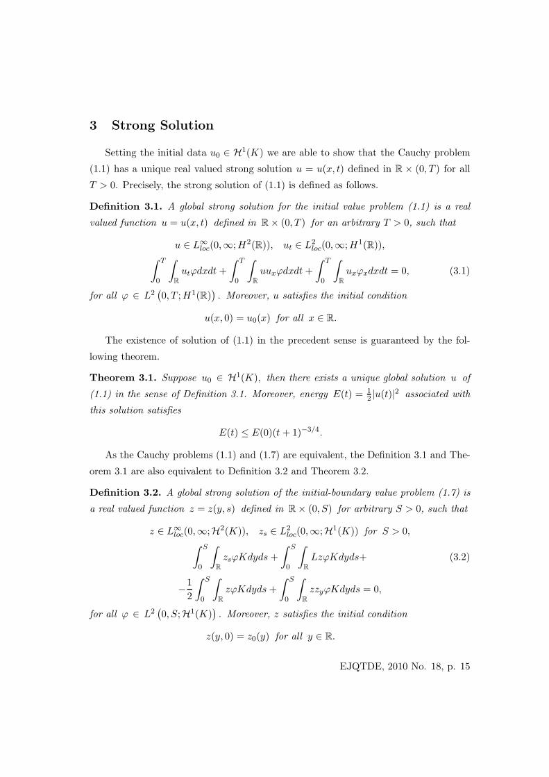
3 Strong Solution
Setting the initial data u0 ∈ H1(K) we are able to show that the Cauchy problem
(1.1) has a unique real valued strong solution u = u(x, t) defined in R × (0, T ) for all
T > 0. Precisely, the strong solution of (1.1) is defined as follows.
Definition 3.1. A global strong solution for the initial value problem (1.1) is a real
valued function u = u(x, t) defined in R × (0, T ) for an arbitrary T > 0, such that
u ∈ L∞loc(0,∞;H2(R)), ut ∈ L2
loc(0,∞;H1(R)),∫ T
0
∫
R
utϕdxdt +
∫ T
0
∫
R
uuxϕdxdt +
∫ T
0
∫
R
uxϕxdxdt = 0, (3.1)
for all ϕ ∈ L2(0, T ;H1(R)
). Moreover, u satisfies the initial condition
u(x, 0) = u0(x) for all x ∈ R.
The existence of solution of (1.1) in the precedent sense is guaranteed by the fol-
lowing theorem.
Theorem 3.1. Suppose u0 ∈ H1(K), then there exists a unique global solution u of
(1.1) in the sense of Definition 3.1. Moreover, energy E(t) = 12 |u(t)|2 associated with
this solution satisfies
E(t) ≤ E(0)(t + 1)−3/4.
As the Cauchy problems (1.1) and (1.7) are equivalent, the Definition 3.1 and The-
orem 3.1 are also equivalent to Definition 3.2 and Theorem 3.2.
Definition 3.2. A global strong solution of the initial-boundary value problem (1.7) is
a real valued function z = z(y, s) defined in R × (0, S) for arbitrary S > 0, such that
z ∈ L∞loc(0,∞;H2(K)), zs ∈ L2
loc(0,∞;H1(K)) for S > 0,∫ S
0
∫
R
zsϕKdyds +
∫ S
0
∫
R
LzϕKdyds+ (3.2)
−1
2
∫ S
0
∫
R
zϕKdyds +
∫ S
0
∫
R
zzyϕKdyds = 0,
for all ϕ ∈ L2(0, S;H1(K)
). Moreover, z satisfies the initial condition
z(y, 0) = z0(y) for all y ∈ R.
EJQTDE, 2010 No. 18, p. 15

The existence of solutions of the system (1.7) will be also shown by means of Faedo-
Galerkin method and by using the special basis defined as solutions of spectral problem
(2.4) and the first eigenfunction ω1 of L such that {ω1}⊥ ={v ∈ L2(K); (ω1, v) = 0
}.
Under these conditions one defines VN as in Section 2. Now we state the following
theorem.
Theorem 3.2. Suppose z0 ∈ H1(K) ∩ {ω1}⊥, then there exists a unique solution z
of (1.7) in the sense of Definition 2.2, provided |z0y| < 1/4√
6C1 holds. Moreover, the
energy E(s) = 12 |z(s)|2 satisfies
E(s) ≤ E(0) exp [−s/4] .
Since Theorems 3.1 and 3.2 are equivalent it is suffices to prove Theorem 3.2.
Proof of Theorem 3.2 - We need to establish two estimates. In fact,
Estimate 3. Setting ω = LzN (s) ∈ VN in (2.6)1, it yields
1
2
d
ds|zN
y (s)|2 + |LzN (s)|2 ≤1
8|zN (s)|2 +
1
2|LzN (s)|2 +
∣∣∣∫
R
zN (s)zNy (s)LzN (s)Kdy
∣∣∣R
.
Next, we will find the upper bound of the last term on the right-hand side of the above
inequality. In fact, by using Holder inequality, Proposition 2.2-items (b), (c) and (d)
we can write
∣∣∣∫
R
zN (s)zNy (s)LzN (s)Kdy
∣∣∣R
≤ C1
√6∣∣zN
y (s)∣∣ ∣∣LzN (s)
∣∣2 .
From this we have
1
2
d
ds|zN
y (s)|2 +1
8|LzN (s)|2 +
1
8
(|LzN (s)|2 − |zN (s)|2
)+
|LzN (s)|2(1
4−
√6C1|zN
y (s)|)≤ 0.
(3.3)
Use a similar argument as in Estimate 1 we are able to prove that
1
8
(|LzN (s)|2 − |zN (s)|2
)≥ 0 for all N ∈ N. (3.4)
EJQTDE, 2010 No. 18, p. 16

In fact, note that
1
8
(|LzN (s)|2 − |zN (s)|2
)=
1
8(g1N (s))2
(λ2
1 − 1)
+1
8
N∑
j=2
(gjN (s))2(λ2
j − 1).
From (2.9) we have
N∑
j=2
(gjN (s))2(λ2
j − 1)≥ 0 and g1N (s) = 0 for all s and N.
From this we obtain (3.4), see Estimate 1. Since (3.4) is true, the inequality (3.3) is
reduced to
1
2
d
ds|zN
y (s)|2 +1
8|LzN (s)|2 + |LzN (s)|2
(1
4−√
6C1|zNy (s)|
)≤ 0. (3.5)
Next, proceeding as (2.12) we will prove that
|zNy (s)| < 1/4
√6C1 for all s ≥ 0. (3.6)
Therefore, by using (3.6) in (3.5), it yields
1
2
d
ds|zN
y (s)|2 +1
8|LzN (s)|2 ≤ 0.
Integrating from 0 to s and using the hypothesis on the initial data we obtain
|zNy (s)|2 +
1
4
∫ s
0|LzN (τ)|2dτ ≤ |z0y|2 <
1
4√
6C1
. (3.7)
Estimate 4. Setting ω = zNs (s) ∈ VN in (2.6)1, it yields
|zNs (s)|2 = −
(LzN (s), zN
s (s))
+1
2
(zN (s), zN
s (s))−(zN (s)zN
y (s), zNs (s)
).
Next, we will estimate the three inner product on the right-hand side of the above
identity. In fact, by usual inequalities and Proposition 2.2 we have
|zNs (s)|2 ≤ C2
2
[∣∣LzN (s)∣∣+ 1
2
∣∣zN (s)∣∣+∣∣zN
y (s)∣∣2]2
,
where C2 = max{1,√
3C1}. From this we get a constant C > 0 independent of N and
s such that∫ S
0
∣∣zNs (s)
∣∣2 ds ≤ C, (3.8)
EJQTDE, 2010 No. 18, p. 17

where C depends on the constant of Estimate (3.7), that is, 1/4√
6C1 and of the con-
stants of immersions established in Proposition 2.2.
From (3.7) and (3.8) we can take the limit on the approximate system (2.6). In
fact, the analysis of the limit as N −→ ∞ in the linear terms of (2.6) is similar to
those of Section 2. However, the nonlinear term is made as follows. From (3.7), (3.8)
and Aubin-Lions theorem one extracts subsequences of (zN ), which will be denoted by
(zN ), such that
∣∣∣∣∣∣∣∣∣∣∣
zN ⇀ z weak in L2(0, S;H2(K)
)as N −→ ∞,
zN → z strong in L2(0, S;L2(K)
)as N −→ ∞,
zNy → zy strong in L2
(0, S;L2(K)
)as N −→ ∞,
zNs ⇀ zs weak in L2
(0, S;L2(K)
)as N −→ ∞.
(3.9)
From usual inequalities and Proposition 2.2 one has
∫
R
∣∣zNy (s)zN (s) − zy(s)z(s)
∣∣2RKdy =
∫
R
∣∣[zNy (s) − zy(s)
]zN (s) + zy(s)
[zN (s) − z(s)
]∣∣2RKdy ≤
2∣∣zN (s)
∣∣2L∞(R)
∣∣zNy (s) − zy(s)
∣∣2 + 2 |zy(s)|2∣∣zN (s) − z(s)
∣∣2 ≤
C[∣∣zN
y (s) − zy(s)∣∣2 +
∣∣zN (s) − z(s)∣∣2].
Taking (3.9) in this inequality, it yields
∫ S
0
∣∣zNy (s)zN (s) − zy(s)z(s)
∣∣2 ds ≤
C
∫ S
0
[∣∣zNy (s) − zy(s)
∣∣2 +∣∣zN (s) − z(s)
∣∣2]ds −→ 0 as N −→ ∞.
(3.10)
Therefore, one has
zNy z
N −→ zyz strong in L2(0, S;L2(K)
)as N −→ ∞
Thus, the proof of Theorem 3.2 is completed by using a similar argument as in
Section 2.
Finally, the uniqueness of solutions and the exponential decay rate of the energy are
established in a similar way as in Section 2
EJQTDE, 2010 No. 18, p. 18

4 Regularity of Strong Solutions
Our goal here is to prove a result of regularity for strong solutions established in
Section 3. We will achieve this goal by means of the following regularity result
Theorem 4.1. Let z = z(y, s) be a strong solution of problem (1.7), which is guaran-
teed by Theorem 3.2, then z ∈ C0([0, T ];H1(K)
).
Proof: We will show that z is the limit of a Cauchy sequence. In fact, suppose
M, N ∈ N fixed with N > M and zN , zM are two solutions of (1.7). Thus, vN =
zN − zM satisfies
vNs (s) + LvN (s) − 1
2vN (s) = PM
(zM (s)zM
y (s))− PN
(zN (s)zN
y (s))
in L2(K).
Therefore, from (2.6), one has that
(vNs (s), ω
)+(LvN (s), ω
)− 1/2
(vN (s), ω
)=
(PM
(zM (s)zM
y (s))−(PN
(zN (s)zN
y (s)), ω), ω),
(4.1)
for all ω ∈ V N ⊂ L2(K), where PN , PM are projection operators defined in L2(K) with
values in V N , VM respectively.
Estimate 5. Setting ω = vN (s) ∈ VN in (4.1) we get
1
2
d
ds
∣∣vN (s)∣∣2 +
∣∣vNy (s)
∣∣2 − 1
2
∣∣vN (s)∣∣2 ≤
∣∣∣PN
(zN (s)zN
y (s) − z(s)zy(s))
+ PN (z(s)zy(s))−
PM (z(s)zy(s)) + PM
(z(s)zy(s) − zM (s)zM
y (s)) ∣∣∣∣∣vN (s)
∣∣ ≤∣∣zN (s)zN
y (s) − z(s)zy(s)∣∣2 + |PN (z(s)zy(s)) − PM (z(s)zy(s))|2 +
∣∣z(s)zy(s) − zM (s)zMy (s)
∣∣2 +3
4
∣∣vN (s)∣∣2 .
Integrating form 0 to S one has
1
2
∣∣vN (s)∣∣2 +
∫ S
0
∣∣vNy (s)
∣∣2 ds ≤ 1
2
∣∣vN0
∣∣2 +
∫ S
0
∣∣zN (s)zNy (s) − z(s)zy(s)
∣∣2 ds+∫ S
0|PN (z(s)zy(s)) − PM (z(s)zy(s))|2 ds+
∫ S
0
∣∣z(s)zy(s) − zM (s)zMy (s)
∣∣2 ds+5
4
∫ S
0
∣∣vN (s)∣∣2 ds.
(4.2)
EJQTDE, 2010 No. 18, p. 19
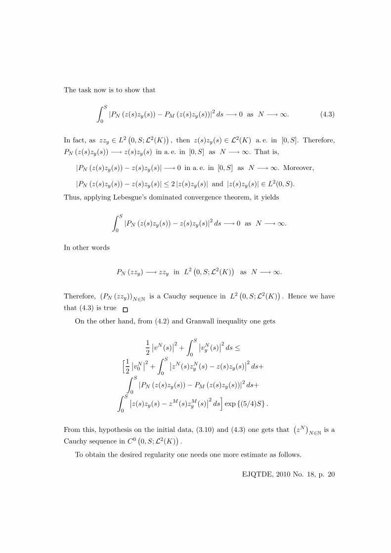
The task now is to show that
∫ S
0|PN (z(s)zy(s)) − PM (z(s)zy(s))|2 ds −→ 0 as N −→ ∞. (4.3)
In fact, as zzy ∈ L2(0, S;L2(K)
), then z(s)zy(s) ∈ L2(K) a. e. in [0, S]. Therefore,
PN (z(s)zy(s)) −→ z(s)zy(s) in a. e. in [0, S] as N −→ ∞. That is,
|PN (z(s)zy(s)) − z(s)zy(s)| −→ 0 in a. e. in [0, S] as N −→ ∞. Moreover,
|PN (z(s)zy(s)) − z(s)zy(s)| ≤ 2 |z(s)zy(s)| and |z(s)zy(s)| ∈ L2(0, S).
Thus, applying Lebesgue’s dominated convergence theorem, it yields
∫ S
0|PN (z(s)zy(s)) − z(s)zy(s)|2 ds −→ 0 as N −→ ∞.
In other words
PN (zzy) −→ zzy in L2(0, S;L2(K)
)as N −→ ∞.
Therefore, (PN (zzy))N∈Nis a Cauchy sequence in L2
(0, S;L2(K)
). Hence we have
that (4.3) is true
On the other hand, from (4.2) and Granwall inequality one gets
1
2
∣∣vN (s)∣∣2 +
∫ S
0
∣∣vNy (s)
∣∣2 ds ≤[12
∣∣vN0
∣∣2 +
∫ S
0
∣∣zN (s)zNy (s) − z(s)zy(s)
∣∣2 ds+∫ S
0|PN (z(s)zy(s)) − PM (z(s)zy(s))|2 ds+
∫ S
0
∣∣z(s)zy(s) − zM (s)zMy (s)
∣∣2 ds]exp {(5/4)S} .
From this, hypothesis on the initial data, (3.10) and (4.3) one gets that(zN)N∈N
is a
Cauchy sequence in C0(0, S;L2(K)
).
To obtain the desired regularity one needs one more estimate as follows.
EJQTDE, 2010 No. 18, p. 20

Estimate 6. Setting ω = LvN (s) ∈ VN in (4.1) we get
1
2
d
ds
∣∣vNy (s)
∣∣2 +∣∣LvN (s)
∣∣2 − 1
2
∣∣vNy (s)
∣∣2 ≤∣∣∣PN
(zN (s)zN
y (s) − z(s)zy(s))
+ PN (z(s)zy(s))−
PM (z(s)zy(s)) + PM
(z(s)zy(s) − zM (s)zM
y (s)) ∣∣∣∣∣LvN (s)
∣∣ ≤∣∣zN (s)zN
y (s) − z(s)zy(s)∣∣2 + |PN (z(s)zy(s)) − PM (z(s)zy(s))|2 +
∣∣z(s)zy(s) − zM (s)zMy (s)
∣∣2 +3
4
∣∣LvN (s)∣∣2 .
Integrating from 0 to S and using Granwall inequality, one gets
1
2
∣∣vNy (s)
∣∣2 +
∫ S
0
∣∣LvNy (s)
∣∣2 ds ≤[12
∣∣vN0y
∣∣2 +
∫ S
0
∣∣zN (s)zNy (s) − z(s)zy(s)
∣∣2 ds+∫ S
0|PN (z(s)zy(s)) − PM (z(s)zy(s))|2 ds+
∫ S
0
∣∣z(s)zy(s) − zM (s)zMy (s)
∣∣2 ds]exp {(5/4)S} .
From this, hypothesis on the initial data, (3.10) and (4.3) one gets that(zN)N∈N
is
a Cauchy sequence in C0(0, S;H1(K)
). Thus, we have the desired regularity. And
therefore the proof of Theorem 4.1 is ended
Acknowledgment We want to thank the anonymous referee for a careful reading
and helpful suggestions which led to an improvement of the original manuscript.
References
[1] Aubin, J. P., Un theoreme de compacite, C.R. Acad. Sci. Paris, 256 (1963), pp.
5042–5044.
[2] Bateman, H., Some recent researches on the motion of fluids, Mon. Water Rev.,
43 (1915), pp. 163–170.
[3] Brezis, H., Analyse Fonctionelle (Theorie et Applications), Dunod, Paris (1999).
EJQTDE, 2010 No. 18, p. 21

[4] Browder, F. E., Problemes Non-Lineaires, Press de l’Universite de Montreal,
(1966), Canada, Montreal.
[5] Burgers, J. M., Application of a model system to illustrate some points of the
statistical theory of free turbulence, Proc. Acad. Sci. Amsterdam, 43 (1940), pp.
2–12.
[6] Burgers, J. M., A mathematical model illustrating the theory of turbulence), Adv.
App. Mech., Ed. R. V. Mises and T. V. Karman, 1 (1948), pp. 171–199.
[7] Coddington, R. E. & Levinson, N., Theory of ordinary differential equations, Mac-
Graw Hill, N.Y. 1955.
[8] Courant, R. & Friedrichs, K. O., Supersonic flow and shock waves Interscience,
New York, 1948.
[9] Courant, R. & Hilbert, D., Methods of mathematical physics, vol. II, Interscience,
New York, 1962.
[10] Hopf, E., The partial differential equation ut + uux = ǫuxx, Comm. Pure Appl.
Math., 3 (1950), pp. 201–230.
[11] Escobedo, M. & Kavian, O., Variational problems related to self-similar solutions
of the heat equation, Nonlinear Analysis, TMA, Vol. 11, No. 10 (1987), pp. 1103–
1133.
[12] Kurtz, J. C., Weighted Sobolev spaces with applications to singular nonlinear bound-
ary value problems, J. Diff. Equations, 49, (1983), pp. 105–123.
[13] Lax, P., Hyperbolic systems of conservation laws and the mathematical theory of
shock waves, SIAM - Regional conference series in applied mathematics, No. 11,
pp. 1–47, (1972).
[14] Lions, J. L., Problemes aux limites dans les equations aux derivees partielles, Oeu-
vres Choisies de Jacques Louis Lions, Vol. I, EDP Sciences Ed. Paris, 2003.
[15] Lions, J. L., Quelques methodes de resolution des problemes aux limites non lin-
eaires, Dunod, Paris (1969).
EJQTDE, 2010 No. 18, p. 22

[16] Schwartz, L., Methodes mathematiques pour les sciences physiques, Hermann,
Paris, France, 1945.
[17] Stoker, J. J., Water waves, Interscience, New York, 1957
[18] Strauss, W. A., Existence of solitary waves in higher dimensions, Communs Math.
Phys., 55, (1977), pp. 149–162.
(Received December 29, 2009)
EJQTDE, 2010 No. 18, p. 23