on the zeros and poles of padé approximants to

Numer. Math. 30, 241-266 (1978) Numerische Mathematik �9 by Springer-Verlag 1978

On the Zeros and Poles of Pad~ Approximants to e ~. III

E. B. Saff*

Department of Mathematics, University of South Florida, Tampa, FL 33620, USA

R. S. Varga**

Department of Mathematics, Kent State University, Kent, OH 44242, USA

Summary. In this paper, we continue our study of the location of the zeros and poles of general Pad6 approximants to e =. We state and prove here new results for the asymptotic location of the normalized zeros and poles for sequences of Pad6 approximants to e ~, and for the asymptotic location of the normalized zeros for the associated Pad6 remainders to e =. In so doing, we obtain new results for nontrivial zeros of Whittaker functions, and also generalize earlier results of Szegt~ and Olver.

Sub jec t Classi f icat ions . AMS(MOS): 41A20; CR: 5.13.

1. Introduction

The purpose of this paper is to state and prove new results on the location of limit points for the zeros and poles for sequences of normalized Pad6 approximants to e ~, as announced in [12], and for the zeros of the associated normalized Pad6 remainders to e =. We also present a new result on the angular distribution of these limit points of zeros and poles.

What has strongly motivated this work is an incisive article by Szeg/5 [14],

which considers the zeros of the partial sums s,(z)..= ~ zk/k! of the Maclaurin k=O

expansion for e =. Szeg6 [-14] showed that ~ is a limit point of zeros of the sequence of normalized partial sums {s,(nz)},~=l iff

12el-el=l and 1s (1.1)

(This result was obtained later independently by Dieudonn6 [2].) Moreover, Szeg~5 [14] showed that ~ is a nontrivial (i.e., nonzero) limit point of zeros of the normalized remainders { e "z - s , (nz ) } ~= 1 iff

[2e l -e [= l and 121>1. (1.2)

* Research supported in part by the Air Force Office of Scientific Research under Grant AFOSR-74- 2688 ** Research supported in part by the Air Force Office of Scientific Research under Grant AFOSR-74- 2729, and by the Energy Research and Development Administration (ERDA) under Grant EY-76-S-02- 2075

0029-599X/78/0030/0241/$05.20

242 E.B. Saff a n d R.S. V a r g a

The connection of Szeg6's result with Pad6 approximations to e ~ is evident in that s,(z) is the (n,0)-th Pad6 approximant to e ~. Our new results, giving sharp generalizations of Szeg~5's results to the asymptotic distribution of zeros and poles of more general sequences of Pad6 approximants to e ~, will be stated explicitly in w 2, with their proofs being given in w167 3-6. For the remainder of this section, we introduce necessary notation and cite needed known results.

As in [9], for any nonnegative integers n and v, let R,,~(z) denote the Pad6 rational approximant of type (n, v) to e ~, and write

R.,~(z)=P.,~(z)/Q.,~(z),

where the degrees of P., v(z) and Q., ~(z) are respectively n and v, and where Q.,~(0) = 1. It is explicitly known (cf. Perron [8, p. 433]) that

n T ~ k P.,~(z) = S" (n+v-k ) !n ! z~ �9 k~=O (n+ v)! k! (n - k)!' ~ ( n + v - k ) ! v ! ( - z ) k

Q,,~(Z)=k=O (n+ v)! kt (v -k) ! ' (1.3)

so that

Q.,~(z)=Pv,.(-z). (1.4)

Because of this identity (1.4), results on the zeros of Pad6 approximants easily translate into results on the poles of Pad6 approximants. In addition, it is known (cf. Perron [8, p. 436]) that the Pad6 remainder e~-R.,~(z) has the representation

Q., v(z) {e ~ - R., v(z)} = e~Q., v(z) - P., ~(z) (__ l ) vZn+v+l 1

(n+v)! ! et~(1-t)"t~dt" (1.5)

Essential for the statements and proofs of our main results are the following recent results on zeros of Pad6 approximants to eL

Theorem 1.1. (Saff and Varga [9-11]). For every v > 0, n > 2, the Pad6 approximant R,,~(z) to e ~ has all its zeros in the infinite sector

( ~ - ~ - ~ 1 ~ S"'v:={ z: [ a r g z l > c ~ n+v ]3"

Furthermore, on defining generically the infinite sector S~, 2 > 0, by

S~:={z: larg z[ > cos- 1 ( 1 ~ ) } , (1.6)

z oo satisfying consider any sequence of Pad6 approximants {R.~,vj( )}j= 1

l imnj= + ~ , and limVJ=a, (1.7) j ~ ~ j~ oonj

On the Zeros and Poles of Pad6 Approximants to e ~. III 243

for any a with 0 < a < ~ . Then, for any e with 0 < e < a, {R,~, ~j(z)}s= 1 has infinitely many zeros in S,_~, and only finitely many zeros in the complement of S,_~, and S, is the smallest sector of the form larg zl > z, r > 0, with this property.

Theorem 1.2. (Saff and Varga [12]). For any n > 1 and any v > 0, all the zeros of the Pad6 approx imant R,. ~(z) lie in the annulus

(n+v)p<lz l<n+v+4/3 ( # - 0.278465), (1.8)

where p is the unique positive root o f # e 1 +" = 1. Moreover , the constant p in (1.8) is best possible in the sense that

# = inf {Izl/(n+v): R.,v(z)=0}. n> l, v>=O

We remark that because of the identity in (1.4), the inequality (1.8) also applies to the poles of any Pad6 approx imant R,,~(z) with n > 0 and v > 1.

Theorem 1.3. (Saff and Varga [10]). For any a with 0 < a < o % consider any sequence of Pad6 approximants {R,~,~j(z)}T= 1 for e z for which (1.7) is satisfied. Then, R,~,,j(z) has zeros of the form

{ ( n j + v ~ + l ) e x p _ _ . i c o s - l \ n j + v j + l - +O((nj+vj+l)l/3), as j - - .oo. (1.9)

2. Statements of New Results

We list and discuss our new results in this section. To begin, for any nonnegat ive integers n and v, we have from (1.5) that the Pad6 remainder to e z, e z - R , , ~(z), has a trivial zero at z =0. As our first result, which is necessary for the proof of one of our main results, we state

Proposition 2.1. For any nonnegat ive n and v with n + v > 0, let z be any nontrivial zero of the Pad6 remainder, eZ-R.,v(z), to e ~. Then,

Iz] > {(n + v)(n + v + 2)} 1/2. (2.1)

The proof of Proposi t ion 2.1 will be given in Section 3. We remark that the Pad6 remainder e ~ - R , , v(z) is known to have infinitely many zeros for any n > 1 and any v > 0, and such remainders have been studied in the literature (cf. Szeg5 [14] and Wynn 1-18]),

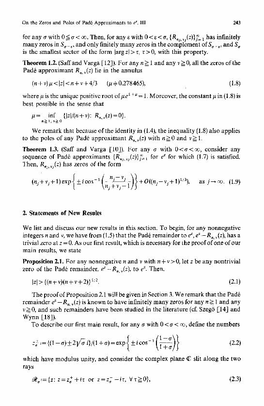
To describe our first main result, for any a with 0 < a < 0% define the numbers

1-o-

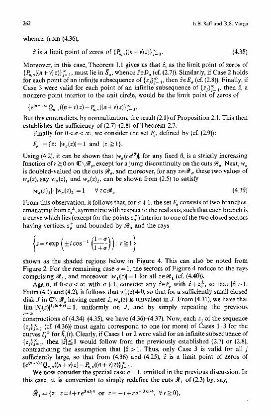
which have modulus unity, and consider the complex plane ~ slit along the two rays

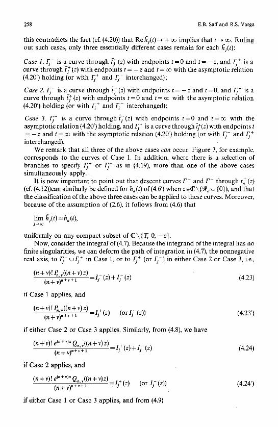
~ . ' = { z : z=z+~+iz or z = z 2 - i z , V~>O}, (2.3)

244 E.B. Saff and R.S. Varga

as shown in Figure 1. Now, the function

1/ g~(z).'= [/ 1 + z 2 \1 + a ] (2.4)

has z + and z~- as branch points, which are the finite extremities o f ~ . On taking the principal branch for the square root, i.e., on setting g~(0)= 1 and extending g~ analytically on this double slit domain ~ \ ~ , then g~ is analytic and single-valued on C \ ~ . Next, it can be verified that +_z+g~(z) does not vanish on C \ ~ .

f i -9[- -..~ 4-

I / I \\

\ I / \ I /

Fig. 1

2 2a

Thus, we define, respectively, (1 + z + g . (z)) 1+* and (1 - z + g . (z)) 1 + * by requir- 2 2a

ing that their values at z = 0 be the positive real numbers 21 +* and 21 +*, and by analytic continuation. These functions are also analytic and single-valued in �9 \ ~ . . With these conventions, we set

4a (T~) z e *~(=) w~(z).- 2 2~ , 0 < a < ~ , (2.5)

(l +a)( l + z +g~(z))a +~'(1-z +g~(z))l +'*

and it follows that w~ is analytic and single-valued on ~ \ ~ . Next, on letting a ~ 0 in (2.5), we verify that Wo(Z):= l im w,(z) satisfies

o '~0

Wo(Z)=ze 1-z for R e z < l , and

Wo(Z)=(ze l - z ) - 1 for R e z > 1. (2.5')

With these definitions, we come to our first main result, which is a strengthened form of a result announced in [12]. Its p roo f is given in w 4.

Theorem 2.2. For any a with 0 < a < o% consider any sequence of Pad6 approximants {R,j.~j(z)}j~ 1 to e ~ for which

l im nj = + or, and lira (vJni) = a, (2.6)

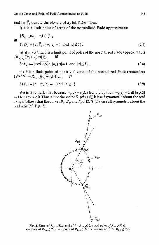
On the Zeros and Poles of Pad6 Approximants to e ~. Ill 245

and let S, denote the closure of So (cf. (1.6)). Then,

i) ~ is a limit po in t of zeros of the no rma l i zed Pad6 app rox iman t s

{R. j . ,~j ((n~. + v j)z)}~= 1 iff

~Do:={zeS~: Iw . ( z ) t= l and tzt_---1}; (2.7)

ii) if a > O, then ~ is a limit po in t of poles of the normal i zed Pad6 app rox iman t s {R.j,.~j((nj + v~) z)}/=, iff

~eE~ := {zer : Iwo(z)l = 1 and Izl_-__ 1}; (2.8)

iii) 2 is a l imit po in t of nont r iv ia l zeros of the no rma l i zed Pad6 remainders {e ("j +~J)" - R,,~. ~j ((nj + vj) z)}7= 1 iff

2~F,, , = { z : IWo(Z)l=l and Iz l> l} . (2.9)

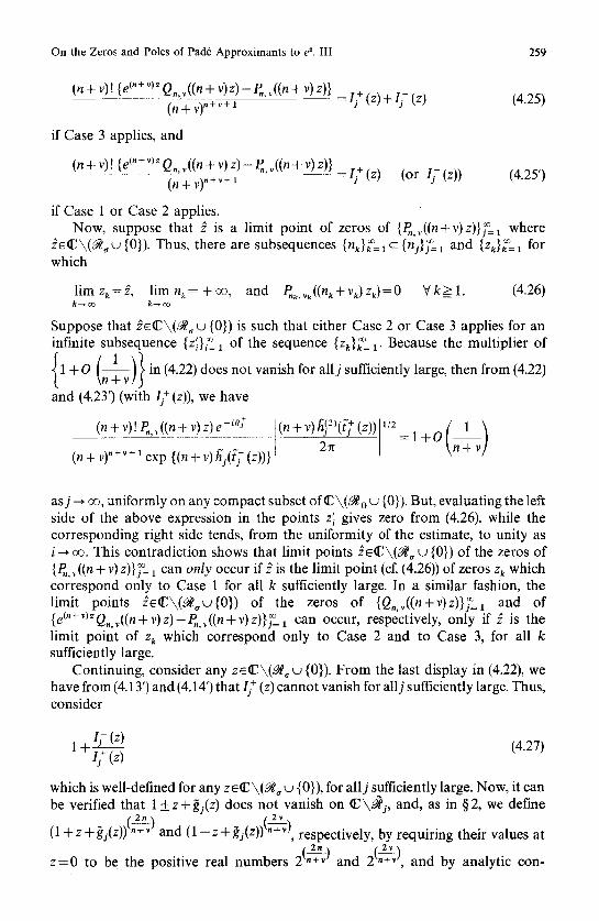
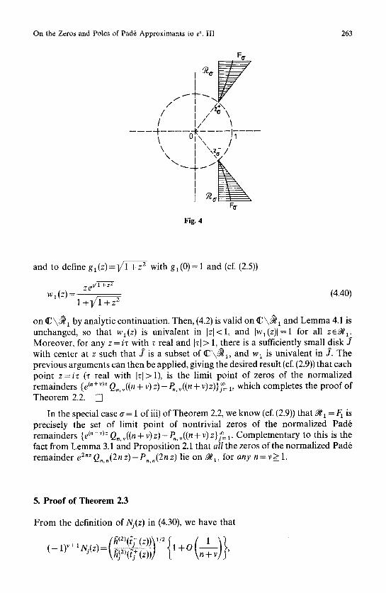
W e first r emark that because Wo(Z) = w,(z-) f rom (2.5), then Iw,(z)] = 1 iff Iwo(z--)l = 1 for any a >_ 0. Thus, since the sector S o (cf. (1.6)) is itself symmetr ic abou t the real axis, it follows that the curves D~, E, , and F o of(2.7)-(2.9) are all symmetr ic abou t the real axis (cf. Fig. 2).

5/3

:i / /

D1/,3 /

+ 113

\ \ 1

Fig. 2. Zeros of R24.s(32z ) and e32~-Rz4.s(32z), and poles of R24.s(32z ). �9 =zeros oi" R2a s(32z) + =poles of R2a s(32z) x =zeros of e3ZZ-Rz4.s(32z)


We next remark that in the special case of Theorem 2.2 with a = 0 and, in addition, with vj = 0 and n i = j for all j > 1, parts i) and iii) of Theorem 2.2 reduce respectively to Szeg6's result (1.1) and (1.2), since the normalized sequence of approximants in this case, {Rj, 0(jz)}j% 1, is just {s,(nz)},~176 r Furthermore, for the choice vj = j = nj for all j > 1, (2.6) is satisfied with a = 1, and in this case, the curves D a and Ea, after rotations of n/2, form the boundaries of the eye-shaped domain considered by Olver [6, p. 336] in his asymptotic expansions of Bessel functions.

To illustrate the result of Theorem 2.2, consider the sequence of Pad6 approximants {R3m,ra(4mz)}~= 1 for which a = 1/3 from (2.6). In Figure 2, we have graphed DI/3, E1/3, and port ions of the two branches ofF1/3, along with the 24 zeros and 8 poles of the normalized Pad6 approximant RE< 8 (32 z), denoted respectively by *'s and + 's . In Figure 2, we have also plot ted zeros of the normalized Pad6 remainder e32Z-Rz4,8(32z), which are denoted by x's . Figure 2 shows that Theorem 2.2 quite accurately predicts the zeros and poles ofR, , v((n + v) z), as well as the zeros of the remainder e ~" § v)z _ R,, v((n + v) z), even for relatively small values of n and v. The reader is advised to consult [12] for further graphical illustrations of parts i) and ii) of Theorem 2.2 in the cases a = 0, a = 1, and a = 1/3.

The next result is again motivated by another result of Szeg6 [14]. Its p roof is given in Section 5.

Theorem 2.3. For any a with 0 < a < o% consider any sequence of Pad6 approximants {R.j, vj(z)}~= 1 to e z for which (2.6) is satisfied.

i) If d, is a closed arc of the curve D ~ \ { z f } (cf. (2.7)) with endpoints #1 and/~2 (with a rg#2>a rg /~0 , where w,(#j):=exp(i~bj), j = l , 2 , let z~,tf(d,,) denote the number of zeros z) 1~ of R,j.~j(z) which satisfy arg #z > arg z) l~ => arg #t. Then,

l im z~,a](d~)/n~ = (1 + a)(q~ 2 - q~) (2.10) ~oo 2r~

ii) I f a > 0, and if e, is a closed arc of the curve E , \ { z ~ } (cf. (2.8)) with endpoints #1 and #z where w~(/~j) = exp (i49j),j = 1, 2, let z~,2)(e,,) denote the number of poles zJ z) of R.j, ~, (z) which satisfy arg #2 > arg zJ 2) > arg/~1. Then,

l im ~c,2,)(e~)/v,= (1 + cr) (~b 2 - ~b 1) (2.11) �9 ' " 2rtff J~oO

iii) L e t f , be a Jordan curve which contains in its interior a single closed subarc of one of the branches of F, but no points of D, or E,, let ~b2 - ~b ~ denote the change in the argument of w,(z) as this subarc of F, is traversed in the positive sense, and let ~ta)(L _~3) in f . of the normalized difference e ("j + v~)z .j .~) denote the number of zeros ~ - R.~, ~j((nj + v j) z). Then,

(3) l im z.j (fo! = q 5 2 - ~ , (2.12) j~ oo (nj + vj) 2n

Again, the special case of Theorem 2.3 with a = 0 and, in addition, with v j = 0 and nj=j for all j > 1, is due to Szeg6 [14]. Because wo(z ) = z e 1 -~ for R e z < 1 from

and because Wo( -t---~z / = ___ ie "v'/~, it follows from (2.10)that if {, is the number (2.5'), \ e !

On the Zeros and Poles of Pad6 Approximants to e ". III 247

Table 1. 13., = number of zeros of R3,,,m(z ) in Re z<0

m 13,,, 13,,,/3m

1 3 1 2 6 1 3 9 1 4 10 0.8333 5 13 0.8667 6 16 0.8889 7 17 0.8095 8 20 ~8333 9 23 0.8519

10 26 0.8667

of zeros of s,(z) in R e z < 0 , then, as shown by Szeg/5,

lim n = ~ + ~ n n (a =0). n ~ o 0

In a similar fashion, we can use (2.10) of Theorem 2.3 to deduce the following. If we consider the sequence of Pad6 approximants {R3,,,,,(z)}~= 1, corresponding to the case a = 1/3, then all the zeros of {Ra,.,,,(z)}~= 1, from Theorem 1.1, lie in $1/a = / -

{z: [argz l>cos - l ( �89 Now, let t3m denote the number of zeros of R3,,,,,(z ) in v_ Re z =< 0. Then, to apply Theorem 2.3, the endpoints of the closed arc dl/a in this case are approximate.ly #1 -0 .706999 i and #2 - -0 .706999 i, f rom which it follows that q~t = arg wl/3 (1~1) - 1.193433 rad., and q~z = arg wl/3 (P2) - 5.089 752 rad. Thus, f rom (2.10) we have

13= 2 ( ~ 2 - ~ 0 - 0 . 8 2 6 8 2 4 ( ,=1 /3 ) . (2.13) lim 3 m - 3n m ~ o o

To numerically corroborate this result of (2.13), we give in Table 1 the actual number of zeros of R 3=,,, (z) in Re z < 0 for m = 1 (1)10. Note that the result of the part icular case m = 8 can be checked f rom Figure 2. Al though the convergence of the ratio 13,,/3m is, f rom Table 1, slow, reasonable agreement with (2.13) is evident for small values of m.

The result of(2.10) of Theorem 2.3 can also be formulated as follows. Given any sector S(~l , tpa):={z=reg~ 1~1~___0~---~/2} contained in S~ (cf. (1.6)) with 0 < ~1 < ~02 < 2n, let z~))(r ~'2) denote the number of zeros ofR,j , vj(z) in S(~1, ~b2). Then, assuming (2.6), there is a positive constant m(~O 1, ~2, a) such that

lim tl) n - m (2.10') % (~1,q'2)/j- (~l,qJ2,~), j ~ o o

where the constant m(~,l, ~Oz, tr) can be precisely determined f rom (2.10). We remark that the existence of positive lower bounds for z~lj)(~ t, ~z)/nj for the part icular case tr = 0 and suitable sequences {nj}jZ 1 has been recently announced by Edrei [-3, 4], for more general entire functions than e z.


3. Proof of Proposition 2.1

In this section, we collect some old and some apparently new results on Whittaker functions from which Proposition 2.1 will follow as a special case.

Using the notation

( a ) j : = a ( a + l ) . . . ( a + j - 1 ) , j>=l, (a)o.'= 1,

it is well-known (cf. Olver [7, p. 255]) that the confluent hypergeometric function

tF l (a ;c ; z i ' - V (a)~zJ c 4 : 0 , - 1 , - 2 , " j~=o(c)jj! . . . . .

has the integral representation

iF1 (a; c; z) = F(c) i eZ'( 1 - t) c-a- 1 t ~- 1 dt, (3.1) F(a) r ( c - a) o

when Re r > Re a >0. It is further known (cf. Olver [7, p. 260]) that the related Whittaker functions Mk, m(Z), defined by

Mk, m(Z)'.=e-Z/2Z c/a 1Fl(a;e;z) with k= -c2-a, re=c-12 ' (3.2)

satisfy Whittaker's equation

,, 1 k m2-�88 w ( z ) = { ~ - z + ~ } w ( z ) . (3.3)

Calling any z + 0 for which Mk,m(z)= 0 a nontrivial zero of Mk, m, we next state

Lemma 3.1 (Tsvetkoff [15, Thm. 7]). Let k and m be real with 2m+ 1 >0. Then,

i) if k > 0, all nontrivial zeros of Mk, m(z) satisfy Re z > 2 k; ii) if k < 0, all nontrivial zeros of Mk, re(Z) satisfy Re z < 2 k;

iii) if k = 0, all nontrivial zeros of Mk, re(Z) are purely imaginary. (3.4)

We take this opportunity to point out that Theorem 11 of Tsvetkoff [15], concerning the Whittaker functions Wk, m(Z ), is false. Tsvetkoff asserts in his Theorem 11 that when k>0, Wk, m(Z ), defined (cf. Olver [7, pp. 257 and 260]) by

e - Z / 2 Z - m + l/2 oo Wk'm(z) -- F(m - k + 1/2) ! e - t tin- k- a/2 (t + Z) re+k- 1/2 dt

for Re (m - k + �89 > 0, cannot have zeros in Re z < 0, except on the real axis. To show that this is false, it can be seen from the above definition and from the definition of the Pad6 numerator P,,~(z) in (1.3) that

�9 ( . + ~ )

v! W . - ~ n+v+ l (z )=(n+ v)! e -z/2 z - ~ - Pn, v(z), (3.5) 2 ' 2

On the Zeros and Poles of Pad6 Approximants to e x. III 249

for any nonnegative integers n and v. Now, for n > v, P.,v(z) can have nonreal zeros in R e z > 0 . Indeed, Theorem 2.2 shows that for sequences of Pad6 approximants satisfying (2.6) with 0 < a < ~ , the zeros of the associated normalized sequence of Pad6 numerators have a cont inuum of nonreal limit points in Re z > 0. Tsvetkoffs proof breaks down because he asserts that

where ~ (and hence ~) is a nonreal zero of Wk, m(Z). However, because of the factor e -z/2 in (3.5), the integration above can take place only on a ray in the right-half plane, i.e., only if the zero r satisfies R e z > 0 .

The following result is apparently new.

Proposition 3.2. If m >0, then every nontrivial zero of Mk, m(z ) lies in the region

{ z = x + i y : x > 2 k and y2>xE(4ma-4k2-1 ) /4k2} if k>O; (3.6)

{ z = x + i y : x < 2 k and y2>x2(4m2-4k2 -1 ) /4k2} if k < 0 ; (3.7)

{ z= iy :yZ>(4m2-1 ) } if k = 0 . (3.8)

Proof If w(z) is a solution of the differential equation w"+G(z)w=O, it is well- known (cf. Hille [5, p. 286]) that

~2 Z2 - - Z2

(w(z). w'(z)) [ - j Iw'(t)l 2 dt + j a(t)Iw(t)l 2 dt =0. (3.9)

In the case of the Whittaker equation (3.3), G(z) is given by

k m2- ] 1 G(z) - z z 2 4' (3.9')

Now, let 0 4= z0 = Xo + iyo be a zero of Mk, m (z). The hypothesis rn > 0 implies (cf. (3.2)) that c > 1. Thus, for w(z) = Mk, ~(z), we can integrate from z 1 = 0 to z z = z o in (3.9) to obtain

zO i:O - - S t 2 IM~,m(t)l dt + S G(t)IMk, m(t)l 2 dt=O.

o o

Setting t = p z o, O<=p< 1, this becomes with (3.9')

�9 ]Mk,m(pzo)[ 2 dp = j [Mk,m(PZo)l zodP, o 10220 o

Taking real parts on both sides then gives

1 k (m2_l /4)Xo 40 ] 1 , 2 j [ �9 [Mk,,.I 2 dp = j ]MR, m] X o dp. o v p2(X2o + y ~ ) o


Now, suppose that k>0. Then, from (3.4i) of Lemma 3.1, Rezo=Xo>2k>O, whence

i [ k (m2-l/4)Xo 0 P 2 ( X 2 + Y 2 ) 4~ "[Mk'm[2dp>O'

or equivalently

i I 4k(xg +y~)p-(4mE- 1)x~176 +yg)p2 o 4p2(x2 +y2) 3. [Mk,ml 2 dp >0. (3.10)

The positivity of this integral implies that the quadratic in p in the numerator of the integrand of (3.10) must evidently satisfy

- Xo (xg + yg) p2 + 4 k + yg /p - (4m 2 - 1) Xo > 0

for some p with 0 < p < 1, and this in turn implies that its discriminant must be positive:

16k2(x 2 2 2 2 2 2 2 + Yo) - 4Xo (Xo + Yo)( 4m - l) > 0. (3.11)

Simplifying, (3.11) can be equivalently expressed as

y2 > x2(4m 2 _ 4k 2 _ 1)/4k 2,

which, with x o > 2k, establishes the desired result of (3.6). The proofs of (3.7) and (3.8) are similar. []

We remark that Proposition 3.2 improves and corrects TsvetkolTs Theorem 3 in [16].

Corollary 3.3. If m > 0, then every nontrivial zero of Mk, m(Z ) satisfies

t z [ > ~ - l , whenever 4 m 2 - 1 > 0 . (3.12)

Proof Suppose that k >0, and let 0=~ z o = x o + iy o be a zero of Mk, m. By (3.6) of Proposition 3.2, we have y2 >x2(4m 2 _ 4 k 2 _ 1)/4k 2, or x 2 + y2 >x2(4m 2 _ 1)/4k 2. But as xE>4k 2 also from (3.6), then

x2 +yE>4m2-1,

which gives (3.12). The cases k < 0 and k = 0 are similar. []

Proof of Proposition 2.1. From the identities of (3.1) and (3.2), it follows that [ n + v + 2 ~ 1

M.-v .+v+ 1 ( z ) = ( n + v + 1)! e_Z/2 z~---T~ I ~ eZt( 1 -t)" t v dt v!n! 2 ' 2 0

for any nonnegative integers n and v. Comparison with the integral representation (1.5) thus shows that the above relation can be expressed as

Dv p+v, M,_ v (z)=(-1) v(n+v)!(n+v+ ,. e-Z/2z-t--T-)(e~Q, v(z)-p, v(z)), n + v + l v ! n ! ' '

2 ' 2 (3.13)

On the Zeros and Poles of Pad0 Approximants to eL III 251

whence any nontrivial zero of the Pad6 remainder e~Q,, ~(z)- P,. ~(z) is a nontrivial

zero of M,-~,+~+l(Z), and conversely. Now, in this case, k = ( 2 ~ -~-} and 2 ' 2 \ ~ /

m= - - , from which it follows that m > 0 if n + v > 0 . Applying (3.12) of

Corollary 3.3 gives that the nontrivial zeros of eZQ,,~(z)-P~,~(z) satisfy

I z l > ~ - I =]/(n+v)(n+v+2), thedesiredresul tof (2 .1)ofProposi t ion2.1 []

We remark that for the case of positive integers n and v with n = v, it follows from (3.4iii) of Lemma 3.1 and Proposition 2.1 that every nontrivial zero z of e~Q,,,(z) - P,,,(z) is purely imaginary, with Izl > l /(n + v)(n + v + 2) = 21/n(n + 1).

4. Proof of Theorem 2.2

We begin this section by deriving the following useful property of the function we(z). Lemma 4.1. For any a with 0 < a < oo, the function w~(z), as defined in (2.5)-(2.5'), is univalent in ]zl < 1.

Proof Assume first that 0 < a < ~ . From the definition of g, in (2.4), it follows that

g~(z) = - q <0 implies that z=(1 - a _+ i~)/(1 +~r), where ~ :=] /4a + q(1 +a) 2 satis-

fies ~>2]~- . Hence, by definition (2.3), z ~ , . With this and the fact that the principal branch for the square root is chosen in the definition of g,, then

2 <argg,(z) < ~ V z E r

or equivalently

Reg , (z )>0 V z ~ C \ ~ . (4.1)

Next, a straight-forward calculation based on the definition of w~(z) in (2.5) shows 1 that

zw;(z) - g , ( z ) V z ~ \ ~ . (4.2)

w~(~)

Thus, with (4.1) and the fact that the open unit disk is a subset o f r (as shown in Fig. 1), then

R [zw',(z)'} ^ e ) w~-z) ~ > u in Izl< 1. (4.3)

Moreover, from (2.5'), we directly verify that (4.3) is valid also for a =0. Now, as is well-known (cf. Sansone and Gerretson 1-13, p. 211]), (4.3) implies that w,,(z) is univalent (and starlike) in Izl>l for any 0 < a < o o . []

We remark that Equation (42) arises in a natural way by applying the Liouville transformation [7, p. 191] to the differential Equation (3.3)


We remark that, using (4.3), it can be shown that for any 0 with - lr < 0 < it, there is a unique r~(O) with 0 < r , ( 0 ) < 1 for which Iw~(r,(O)ei~ = 1, and, moreover , that

r,,(O) = 1 only if 0 = ___ cos - 1 ( 1 - ~ ) 1 - a . Hence, the set

G , : = { z e C : lw, (z) l= l and Iz l< l} , (4.4)

is then a well-defined Jordan curve which lies interior to the unit disk, except for its • of(2.2). As a consequence of (2.7) and (2.8), note that G~ = D~ w E~. so that points z,

D~ and E , are well-defined Jordan arcs.

Proof of Theorem 2.2. Because the case a = 0 is similar, consider a fixed a with 0 < a < oo and any sequence of Pad6 numera tors {P,j.~j(z)}~= 1 for which (2.6) is valid:

lim n~ = + oo, and l im (Vj/rlj)= a. j~oo j~oo

For nota t ional simplicity, we now write n and v, respectively, for n~ and vs. By virtue of Theorems 1.1 and 1.2, any zero z of P,.,((n + v)z) satisfies

4 zeS,,~ and O<#<lzl<l+3(n+v~, V j>l .

Consequently, any limit point ~ of zeros of {P,.~((n + v) z)}~~ ~ belongs to the closed set

{zeSt: 0 < / ~ t z l < l } ,

where S, denotes the closure of the sector S~ (cf. (1.6)). To complete the necessity of (2.7) of Theorem 2.2, it remains to show that any such limit point 2 satisfies Iw~(~)l = 1. If 2 = z , + or if ~ = z~, then, as previously noted, 2 e G , , whence Iw~(~)l = 1 from (4.4). Thus, we may assume in what follows that z = 2 satisfies

z e r {0}), (4.5)

• so that in part icular , z + 0 and z ~ z , .

F r o m the explicit formula (1.3), it can be verified that P,,,(z) has the following integral representat ion:

oo

(n+v)!P.,v(z)= S e-t( t+z) "tvdt V j > l , 0

the path of integration being the nonnegat ive respectively by (n + v) z and (n + v)t, and defining

this integral representat ion for P.,v(z) becomes

(n+v)! P.,~((n+v)z)= ~ e(,+v)~(Odt ' Vj>_ 1. (n+v) "+~+t o

real axis. Replacing z and t

Vj > 1, (4.6)

(4.7)

On the Zeros and Poles of Pad6 Approximants to e ~. III 253

As defined,/~j is a multi-valued function of t which is analytic on C \{0, - z}, and for each z~O2\(~,w {0}),/~i(t; z) can be defined to be single-valued and analytic as a function of t on the complement of two suitable cuts T in the t-plane, respectively joining t = 0 and t = - z with infinity. Note however that exp [(n+v)/~i(t)] is analytic and single-valued for all t. Next, from (4.7) and from (1.3)--(1.4), it can also be verified that

(n + v)! e t" + ~ Q., ~((n + v) z) (n+v).+~+l - -~S et"+~hJ~t)dt, Vj>=I, (4.8)

the path of integration being the horizontal ray - z + u for u > 0, and from (1.5),

0 (n+v)! {e~"+~)ZQ,,~((n+v)z)-P,,~((n+v)z)}= ~ e~,+~j~t)dt, V j>I , (4.9) (n+v) "+~+1 _ ~

the path of integration being chosen to be the line segment from - z to 0. Finally, from (2.6), we can define, in analogy with (4.6), the function

h~(t) = h, (t; z):= - t + {ln (t + z) + ~r In t}/(1 + tr), (4.6')

and we now investigate the zeros of/~j(t) and h'~(t). From (4.6), the derivative of/~j is

+ l~{n(t+z)-'+vt-l} , fij(t) = - 1 (n + v)

whose only zeros, t'+ (z) and tj (z), are

~f(z):=�89 (4.10)

where

~ j ( z ) : = ~ l + z2 - 2z ( n - v~ \n + v]" (4.11)

In analogy with the definition of (2.2), the points

are the branch points of ~ , and we can similarly consider the complex plane IE slit along the two rays

~ j : = { z : z=~++i~ or z = ~ ; - i z , V~>0}.

On setting ~j(0) = 1 and extending ~j analytically on ~2\~j , then ~j is analytic and single-valued on ~ \ ~ i for all j > 1, the same being true for the functions t f (z) of (4.10). Note that with (2.4) and (2.6),

lim {+ (z)=a {1-z+_g~(z)}=:t+ (z), V z ~ C \ ( ~ u {0}). (4.12) j ~ o v

and that t + (z) are correspondingly the zeros of h'~(t).


Next, it can be readily verified from the assumption of (4.5) that

i) t+(z)*ts I ii) t~ (z) 4:0 [

iii) t + ( z ) : ~ - z J

Thus, from (4.12),

i) t? (z) :f i f (z)] ii) t'f (z) ,0 /

iii) t~ + (z) 4: - z )

V zOE\(~ / , u {0}). (4.13)

V z O E k ( ~ , u {0}), Vj surf. large. (4.13')

From (4.6), we further have that

h)k)(t)= (k-1)!(-1)k+l {n(t+z)-k+vt-k}, V k > 2 , (4.14) (n + v)

and, on using the case k = 2, it can be verified from (4.5) that

/~j2)(?f (z))4=0 for all j sufficiently large, and (2) • h~ (t~ (z))#:0. (4.14')

In other words, for 0 < o- < oo and for z e l E \ ( ~ u {0}), t~ + (z) and/']- (z) are distinct saddle points (of order one) of ~(t), for all j sufficiently large, and t~ (z) are distinct saddle points (of order one) of h~(t).

We now seek to obtain asymptotic estimates for the integrals of (4.7)-(4.~)), as j ~ 0% by means of the steepest descent method (cf. [1, 7]). To this end, we examine the particular functions

I+(z;6) := S e("+~)hJ(t)dt, (4.15)

where the paths of integration, y+ (6), are respectively the line segments t = i "+ (z) +pc i~ with - 6 < p < +6, where 6 > 0 and where 0 + are to be specified below. Now, for any compact subset K of tE \ ( ~ , u {0}), it can be verified that 3 > 0 can be chosen sufficiently small so that each line segment is a positive distance from t = 0, t = - z, and from the other line segment, independent of the choices of Of, for all zeK, for all j sufficiently large.

Now, for suitable cuts T joining t - 0 and t = - z with infinity but not passing through if(z), we can expand/~l about t'f (z), and as/~'j(t'f (z)=O, we obtain

fi~(t)=~(tf(z))+ ~ (peiO;)kfi)k'(tf(z)), t~yf(6). k=2 k!

Recalling that ~)2)(~f (z))4= 0 for all j sufficiently large, let z f ,= arg/~)2)(~f (z)), and set

Of ,= 2

On the Zeros and Poles of Pad6 Approx iman t s to eL III

For these choices of Of, it follows from the expansion above that

~ ~+_ i o ; "+ p 2 -(2) -+ hj(tj (z)+pe )=~j( t]-(z))-~lh j (t~-(z))[+O(p3),

255

as p ~ 0. Thus, for any compact subset K of C \ ( ~ , w {0}), there exist 3 > 0, A > 0, and J > 0 (in general dependent on K) such that

Re hj(t)- (z) +_ 6 e ̀~ ) < Re/~j(~+ (z)) - A, (4.16).

for all z6K, all j >J . Next, with the change of variables

~ fu where + { @2,(/f (z))lj2+ ~,/2 , > 0 ,

then

u ,~ I ~ ; u e (_, (z)), ?+

and the integral I + (z; 6) of (4.15) can be expressed as

a+exp{(n+v)[ij([+(z))+iO + } ~r { ~ } + S e- "~exp (n+V)k~= du Iff(z;6)= J ] /n+v -~va~w/,; 3 (4.17)

where the sum in the above integral is the same as in the previous display. Thus, on making the Maclaurin expansion of the integrand, integrating termwise, and using

+M

the facts that S e-U2 ukdu = 0 for any odd positive integer k and any M > 0, and that - M

+M

e-"2 du --, ~ as M ~ m, it follows that the integral on the right of (4.17) satisfies - M (cf. [1, 7])

] /~{l+O((n+v)- l )} , as j---r ~ ,

where the modulus of the multiplier of (n + v)-1 in the last term above, is bounded above by

+ (z)))3

However, because of (4.13)-(4.1Y), we see from (4.14) that this sum is bounded above, uniformly on any compact subset of r u {0}), as j ~ ~ . Combining, then

(n + v) 2n 1/2 . Iff(z;8)=e ("+~)~j(-t](~)) /~)2)(~.+ (z)) e '~ {l+O((n+v)- ')} , (4.18)

as j ~ ~ , uniformly on any compact subset of ~ \ ( ~ w {0}).


We now extend both ends of the line segment 7f(6): t=t~+(z)+pe ~~ _ E + =F~,+~(z) and E + = F~,~(z) defined by - 6 < p _< 6, by means of the curves ~, ~ ~,

Fj+~..={tOl2: Imhj(t)=Imhi(t f (z)+6e '~ and

Re/~j(t)__< Re hj(tf. (z) + 6ei~ Fj,~ := { teC: I m ~j(t) = Im/~j(t+ (z) - 6 e ~~ and

Re/~s(t) < Re ~s(t+ (z) - 6e~~ )},

so that E + and Fj~ are descent paths for/~j(t) (cf. [1, 7]). Note that since/~j(t) can j , 1

vanish only for t"--" t~ (z), these descent paths are then well-defined from the local univalence of @ away from t[ (z), for a suitable choice of the cuts T If one of these descent paths, say F.. + passes through t~-(z), then necessarily j , 2 ,

Im ~j(t+ (z) - 6e '~ = Im/Tj (/'j- (z)), (4.19) ~ - ~ ~+ i O f Re/;j( t j (z))<Rehj(tj ( z ) -6e ),

and F~~ then consists of two branches for Re/~(t) < Re ~J(tT)" We select either one of these branches to specify E + In the same manner , we extend both ends of the line j , 2"

segment ~;- (3) by means of the descent paths Fj- 1 and F~,~ in the t-plane. Next, f rom (4.6),

ReB~(t)-- - u + l n l t+z l ~ In It[ , t:=u+iv, (4.20)

so that Re ~j(t)--* - oe implies that t--* - z, t --* 0, or that u ~ + oo. Thus, for any z e r u {0}), C + E -+ ~. 1 and i, 2 are curves in the t-plane, which extend to t = - z or t = 0, or u ~ - ~ . If, say, the curve Fj+I is such that u ~ + ~ , it can be verified that the points t =u + iv of F~]I behave asymptot ica l ly as

K+ X f n l m z K + ] (uls = - , w h e r e

K +.'= Im/~j (/'+ (z) + 6 e '~ (4.20')

Similar asympto t ic relations can be derived if the curves F~,~I and Fj,~ tend to t = 0 or to t = - z .

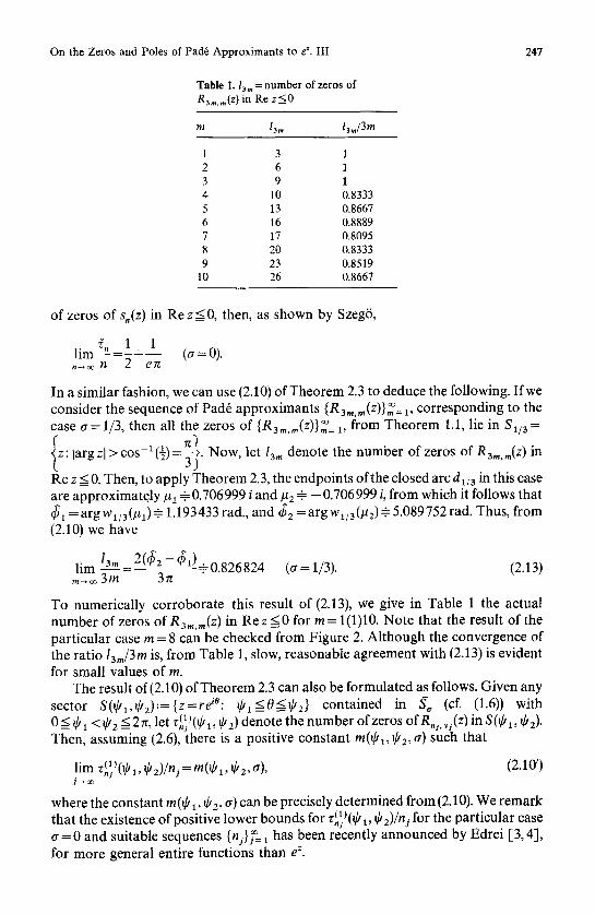
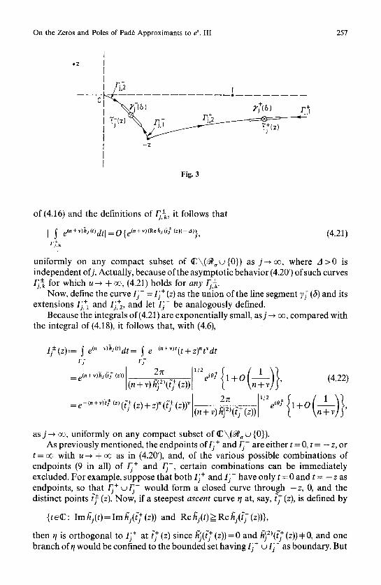
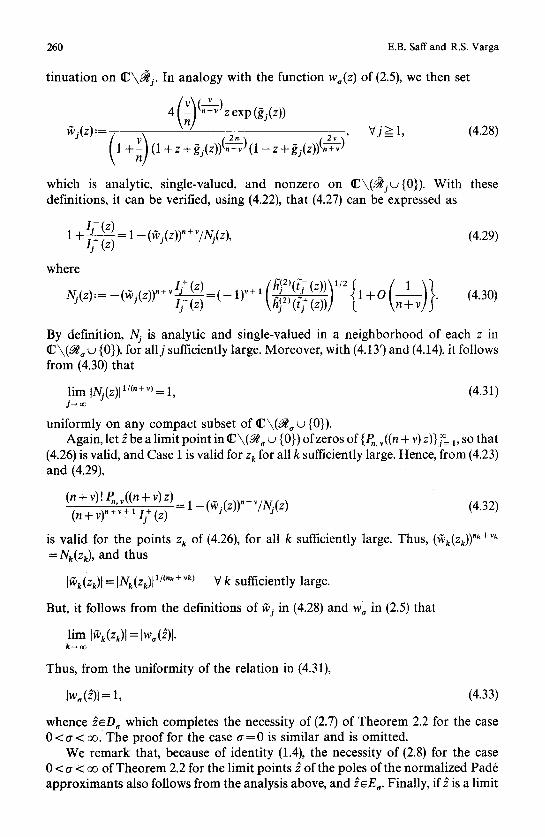
To illustrate this, consider the special case of {P~,j(2jz)}j~= 1 for which ~ = 1 (cf.

(2.6)). In this case, [i~(t) is independent ofj. For the choice z = �89 exp ( 3-4 !) and 6=~ ,

�9 the line segments Vf (3) (shown as double lines) and the curves Fj~ (shown as single curves) are given in Figure 3, where the arrows indicate the direction of increasing Re kTj(t) along these curves.

E + which has either t = 0 or t = - z as an endpoint. Next, consider any curve j,k Using the appropr ia te asympto t ic relation as in (4.20') as t ~ 0 or as t ~ - z , it can be seen that the integrals ~ et"+~)gJt')dt are finite. Moreover , as a consequence

1. k


* Z

I J I I

' 22

-7

7[{ 6 )

T/(z)

Fig. 3

of (4.16) and the definitions of Fj~, it follows that

[ ~ e~"+v)hJ(~ = O {e ~"+*)(R~J(72 m)-~)}, (4.21) • f f j , k

uniformly on any compact subset of r as j ~ o o , where A > 0 is independent ofj. Actually, because of the asymptotic behavior (4.20') of such curves F~.~ for which u ~ + ~ , (4.21) holds for any E +- j,k"

Now, define the curve F~ § = F i + (z) as the union of the line segment 7f (6) and its extensions Fj,+I and E+j,2, and let Fj- be analogously defined.

Because the integrals of(4.21) are exponentially small, as j ~ oo, compared with the integral of (4.18), it follows that, with (4.6),

~ I+(z). '= ~ e(~+~}hJ(~ ~ e-("+v)'(t+z)~t~dt

r: r; 1/2 • (n@v) } 2re io~ 1 + 0 (4.22) e (n

+ v)~lj (z))l(n + v)/~}2)(t-f+ (z)) e

as j ~ o% uniformly on any compact subset of ~ \ ( ~ , • {0}). As previously mentioned, the endpoints of Fj + and Fj- are either t = 0, t = - z, or

t = oo with u ~ + oo as in (4.20'), and, of the various possible combinations of endpoints (9 in all) of Fj + and Fj-, certain combinations can be immediately excluded. For example, suppose that both F~ + and ~ - have only t = 0 and t = - z as endpoints, so that Fj + uF~- would form a closed curve through - z , 0, and the distinct points i f (z). Now, if a steepest ascent curve t/at , say, t f (z), is defined by

{ t e ~ : Imftj(t)=Im~j([+(z))and Rehj(t)>=Re[ij([f (z))},

then r/is or thogonal to F1 + at [+ (z) since/~j([+ (z))=0 and ~J:)([7 (z))4=0, and one branch of~/would be confined to the bounded set having Fj + u Fj- as boundary. But


this contradicts the fact (cf. (4.20)) that Re [b(t) ~ + ~ implies that t ~ ~ . Ruling out such cases, only three essentially different cases remain for each/~j(t):

Case I. F~- is a curve through fj- (z) with endpoints t = 0 and t = - z , and ~+ is a curve through t+ (z) with endpoints t = - z and t = @ with the asymptotic relation (4.20') holding (or with Fj + and ~ - interchanged);

Case 2. Fj- is a curve through tj- (z) with endpoints t = - z and t=0 , and 5 + is a curve through t'+ (z) with endpoints t = 0 and t = ~ with the asymptotic relation (4.20') holding (or with F~ + and Fj- interchanged);

Case 3. F~- is a curve through i'j-(z) with endpoints t = 0 and t = @ with the asymptotic relation (4.20') holding, and Fj + is a curve through ~+(z) with endpoints t = - z and t = ~ with the asymptotic relation (4.20') holding (or with ~ - and ~ + interchanged).

We remark that all three of the above cases can occur. Figure 3, for example, corresponds to the curves of Case 1. In addition, where there is a selection of branches to specify ~+ or F~- as in (4.19), more than one of the above cases simultaneously apply.

It is now important to point out that descent curves F + and F - through t + (z) (of. (4.12))can similarly be defined for h,(t) of (4.6') when z e ~ \ ( ~ w {0}), and that the classification of the above three casesca n be applied to these curves. Moreover , because of the assumption of (2.6), it follows from (4.6) that

lim/~j(t) = h~(t), j ~

uniformly on any compact subset of C \ { T , 0, - z } . Now, consider the integral of (4.7). Because the integrand of the integral has no

finite singularities, we can deform the path of integration in (4.7), the nonnegative real axis, to Fj- w ~ + in Case 1, or to F~ + (or ~ - ) in either Case 2 or Case 3, i.e.,

(n + v)! P.,~((n + v) z) (n+ v) .+~'+1

if Case 1 applies, and

- I + (z) + I~- (z) (4.23)

(n + v) ! P,,v ((n + v) (n + v)" +~ +1 z) =/j+ (z) (or 17 (z))

if either Case 2 or Case 3 applies. Similarly, from (4.8), we have

(4.2Y)

(n + v)! e (" +*)z Q. , , ( (n + v) z) (n+ v),+~+, = I + ( z ) + I j - ( z )


(4.24)

(n + v) l e ~ + v)z Q,,, v((n + v ) z ) (n + v)" +~ + ' - U (z) (or U (z))

if either Case 1 or Case 3 applies, and from (4.9)

(4.24')


(n + v)! {e ("+ ~)" Q,,~ ((n + v ) z ) - P,,~((n + v) z)} = i~ + (z) + I 7 (z) (4.25) (n+v) .+~+1


(n + v)! { e ~" + ~ Q.,~((n + v) z) - P.,~ ((n + v) z)} (n+v),+~+l = I + (z) (or I7(z)) (4.25')

if Case 1 or Case 2 applies. Now, suppose that ~ is a limit point of zeros of {P,,~((n+v)z)}F= 1 where

2 e t E \ ( N , u {0}). Thus, there are subsequences {nk}k~= 1 c {nj}j~= 1 and {Zk}~= 1 for which

lim Zk=2, lira nk= + ~ , and P, . . . . ((nk+Vk)Zk)=O Vk>=l. (4.26) k ~ o 9 k ~ o o

Suppose that 2 ~ r u {0}) is such that either Case 2 or Case 3 applies for an z ~ Because the multiplier of infinite subsequence {z'i}i~= ~ of the sequence { k}*= 1"

I ( tt 1 + 0 ~ v in (4.22) does not vanish for al l j sufficiently large, then from (4.22)

and (4.23') (with I 7 (z)), we have

Lv) (n+v) "+~+' exp {(n+v)rij(t+(z))} 2~t

as j ~ oo, uniformly on any compact subset o f r o u {0}). But, evaluating the left side of the above expression in the points z' i gives zero from (4.26), while the corresponding right side tends, from the uniformity of the estimate, to unity as i ~ oe. This contradiction shows that limit points 2 0 1 2 \ ( ~ u {0}) of the zeros of {P,, v((n + v)z)};= 1 can only occur if 2 is the limit point (cf. (4.26)) of zeros zk which correspond only to Case 1 for all k sufficiently large. In a similar fashion, the

z o~ and of limit points s of the zeros of {Q,,~((n+v))}]=1 {et"+~Q.,~((n+ v)z)-P,,~((n+v)z)}~~ 1 can occur, respectively, only if ~ is the limit point of z k which correspond only to Case 2 and to Case 3, for all k sufficiently large.

Continuing, consider any z ~ r u {0}). F rom the last display in (4.22), we have from (4.13') and (4.14') that I + (z) cannot vanish for allj sufficiently large. Thus, consider

/7 (z) (4.27) 1 -~ 1 / ( z )

which is well-defined for any z ~ r w {0}), for a l l j sufficiently large. Now, it can be verified that 1 +z+~j(z) does not vanish on IU \~ j , and, as in w we define

z + ~j(~))(~"-~) ~j(~))(~-~), (1 + and ( 1 - z + respectively, by requiring their values at ( 2 . ) (2v~

z = 0 to be the positive real numbers 2 ,+v and 2 ,+, ' , and by analytic con-


tinuation on C \ ~ j . In analogy with the function w,,(z) of (2.5), we then set

4 (v)("-~r z exp (~(z))

kj(z).'= (4.28) ( n ) 2, t z~ , ' v j > l '

1 + ( l+z+~j(z))( ,-~)(1-z+gj(z))~,+v j

which is analytic, single-valued, and nonzero on ~ \ (~ jw{0}) . With these definitions, it can be verified, using (4.22), that (4.27) can be expressed as

1 + ~ = 1 - (kj(z))" + V/Nj(z), (4.29) j ( )

where

Ni(z ) :=- (kJ (Z) ' "+v~=(-1 )v+ ' { f i J z ) ( t ] - ( z ) )~ l /2{~ ~z) k ~ ] 1 +O ( ln~v)}. (4.30)

By definition, Nj is analytic and single-valued in a neighborhood of each z in r \ ( ~ , w {0}), for all j sufficiently large. Moreover, with (4.13') and (4.14), it follows from (4.30) that

lim INAz)I 1/(, + , = 1, (4.31) j ~

uniformly on any compact subset of r {0}). Again, let 2 be a limit point in II~\(~, u {0}) of zeros of {P,,~ ((n + v) z)}~= 1, so that

(4.26) is valid, and Case I is valid for z k for all k sufficiently large. Hence, from (4.23) and (4.29),

(n + v)! P.,~((n + v) z) (n + v)" +~ +i/j+ (z) = 1 - (ki(z))" + ~/Nj(z) (4.32)

is valid for the points z k of (4.26), for all k sufficiently large. Thus, (~Vk(Zk)) ''§ = Nk(Zk), and thus

I~(zk)l--INk(z~,)l ~/t''+~k) V k sufficiently large.

But, it follows from the definitions of ~j in (4.28) and w~ in (2.5) that

lim I~k(zk)t = lw~(~)l. k~oo

Thus, from the uniformity of the relation in (4.31),

Iw~(~)l = 1, (4.33)

whence 2eD, which completes the necessity of (2.7) of Theorem 2.2 for the case 0 < a < oo. The proof for the case a = 0 is similar and is omitted.

We remark that, because of identity (1.4), the necessity of (2.8) for the case 0 < a < oo of Theorem 2.2 for the limit points 2 of the poles of the normalized Pad6 approximants also follows from the analysis above, and ~eE,. Finally, if 2 is a limit

On the Zeros and Poles of Pad6 Approximants to e ". III 26l

point of nontrivial zeros of the normalized Pad6 remainders {e ~"+v~ Q,, ~((n + v) z) - P,, ~((n + v) z)};= 1, it is evident from (2.1) of Proposit ion 2.1 that 181 > 1. Moreover, 8 must be the limit o fz k which correspond only to Case 3 for all k sufficiently large. Thus, with Case 3 of (4.25) and the analysis above, [w~(8)[=l, whence 8~F~, completing the necessity of (2.9) of Theorem 2.2.

To complete the proof of Theorem 2.2, we consider the sufficiency of (2.7)- (2.9), and we again assume that 0 < a < ~ . Consider first the set G, of (4.4),

+ and z~- are in G.. But, as a where G,= D , u E , . As previously noted, z~ consequence of (1.9) of Theorem 1.3, it follows, upon normalization, that P,.~((n + v)z) has zeros to~ which satisfy

oJ+--z++o(1), as j ~ .

Thus, both z~ + and z~- are limit points of zeros of {P,,~((n+v)z)}~= v Next, consider any 8~G~ with 84 :z f . F rom the discussion following (4.4), 8 is

then a nonzero interior point of the unit disk, whence 8 ~ C \ ( ~ , ~ {0}). Now, choose any sufficiently small closed disk H having 8 as center such that H c 112\(~ u {0}) and such that H lies interior to the unit disk. F rom (4.31), IN~(z)l ~/~" + ' ~ 1 uniformly on H as j ~ ~ . Noting by definition (4.4) that Iw~(8)l = 1, for each j and each z~H select the (n + v)-th root of N~(z) with argument closest to w,(~). With this choice,

(Nj(z))I/("+v)~ w,,(8) as j ~ ~ ,

uniformly on H. Next, set

f (z) := w~ (z) - w, (8). (4.34)

Because w~ is univalent in Izl< 1 from Lemma 4.1,fhas a unique zero in H at 8, and, moreover, f(z) ~ O. Next, define

fj(z) := ~ ( z ) - (N~(z)) 1/~" + ~) Vj > 1. (4.35)

It follows that {f~(z)}~ ~ converges uniformly to f on H. Hence, by Hurwitz 's Theorem (cf. Walsh [-17, p. 6]),fj has precisely as many zeros in H as does f, for a l l j sufficiently large. But, a s f h a s exactly one zero (at 8) in H, thenf j has precisely one zero, say z j, in H for all j sufficiently large, and moreover

lim zj = 8. (4.36) j ~ ov

Now, f j ( z i )=0 implies from (4.35) and (4.29) that l+( l f ( zy l f - ( z j ) )=O, or equivalently

I~- (z j) + I S (z j) = 0 for all j surf. large. (4.37)

Now, each point zj of the sequence {z~};= 1 corresponds to one (or more) of Cases 1- 3 for the curves Fj-* for h~(t). Suppose then that {Z'k}k~ 1 is an infinite subsequence of {z~};= 1 for which each point z~, corresponds to Case 1. Thus, from (4.23) and (4.37), it follows that

P,,v((n+v)z'k)=O for all k > l ,


whence, from (4.36),

is a limit point of zeros of {P,,v((n + v)z)}j~ 1. (4.38)

Moreover, in this case, Theorem 1.1 gives us that ~, as the limit point of zeros of {P,, ~((n + v)z)};= 1, must lie in S,, whence 2~O, (cf. (2.7)). Similarly, if Case 2 holds for each point of an infinite subsequence of {zj}j~ 1, then ~ E , (cf. (2.8)). Finally, if Case 3 were valid for each point of an infinite subsequence of {zj}j~= 1, then 2, a nonzero point interior to the unit circle, would be the limit point of zeros of

{e~. + ~)z Q,,v((n + v) z) - P.,~ ((n + v) z)}~~ 1.

But this contradicts, by normalization, the result (2.1) of Proposition 2.1. This then establishes the sufficiency of (2.7)-(2.8) of Theorem 2.2.

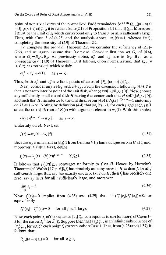
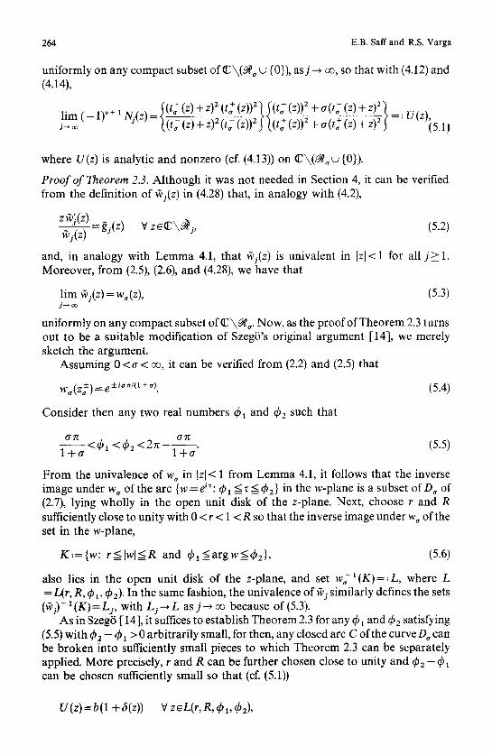
Finally for 0 < cr < oo, we consider the set F~, defined by (cf. (2.9)):

F~,= {z: lw~(z)l = 1 and [z[ > 1}.

Using (4.2), it can be shown that Iw~(re~~ for any fixed 0, is a strictly increasing function of r > 0 on IE\~o, except for a jump discontinuity on the cuts ~ . Next, w, is doubled-valued on the cuts ~ , , and moreover, for any z ~ , , these two values of w,(z), say w,(z)l and w~(z)2, can be shown from (2.5) to satisfy

Iw~(zhl" Iw~(zhl = 1 V zeN~. (4.39)

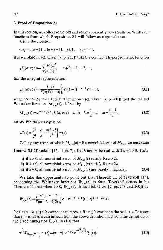
From this observation, it follows that, for a 4:1, the set F, consists of two branches, emanating from z f , symmetric with respect to the real axis, such that each branch is a curve which lies (except for the points z~) interior to one of the two closed sectors

• and bounded by ~ , and the rays having vertices z,

r l} shown as the shaded regions below in Figure 4. This can also be noted from Figure 2. For the remaining case o = 1, the sectors of Figure 4 reduce to the rays comprising ~1, and moreover [wl(z)[ = 1 for all z e ~ l (cf. (4.40)).

Again, if 0 < e < oe with ~r 4:1, consider any 2eF~ with ~+z~, so that I~1 > 1. From (4.1.) and (4.2), it follows that w'~(z),t=O, so that for a sufficiently small closed disk J in C \ ~ having center 9., w~(z) is univalent in J. From (4.31), we have that limlNj(z)l~/~"+~=l, uniformly on J, and by simply repeating the previous

j ~ ~

constructions of (4.34)-(4.35), we have (4.36)-(4.37). Now, each zj of the sequence {zj}[= 1 (cf. (4.36)) must again correspond to one (or more) of Cases 1-3 for the curves F~ • for ~(t). Clearly, if Cases 1 or 2 were valid for an infinite subsequence of {zj}]~ 1, then 121_-< 1 would follow from the previously established (2.7) or (2.8), contradicting the assumption that I~1 > 1. Thus, only Case 3 is valid for all j sufficiently large, so that from (4.36) and (4.25), ff is a limit point of zeros of {e ~" + "~" Q.. , ( (n + v) z) - P., ~((n + v) z)}j~= 1.

We now consider the special case a = 1, omitted in the previous discussion. In this case, it is convenient to simply redefine the cuts ~a of (2.3) by, say,

~ l : = { z : z= i+re 3~/4 or z = - i + r e -3"i/4, Vr>0},

On the Zeros and Poles of Pad~ Approximants to e ~. IlI 263

I - # - . . . - f I ~ I v

, / [ / ~ \ . " I / \

I I i I . . . . . . . . I v - -

\ \ \ "\,,\(g I I '

N Fig. 4

and to define g l ( z ) = ] / 1 + z 2 with g l (0 )= 1 and (cf. (2.5))

zeV1 + z 2

w, (z) = (4.40) 1 + ] / 1 + z 2

on C \ ~ 1 by analytic continuation. Then, (4.2) is valid on ~ \ ~ and L e m m a 4.1 is unchanged, so that wl(z ) is univalent in Iz l< l , and Iwl(z) l= l for all z ~ 1. Moreover , for any z = iz with z real and ]z] > 1, there is a sufficiently small disk J with center at z such that J is a subset of C \ ~ t , and w 1 is univalent in J. The previous arguments can then be applied, giving the desired result (cf. (2.9)) that each point z = i x (z real with ]zl > 1), is the limit point of zeros of the normal ized remainders {e ~"+ ~)= Q.,v ((n + v) z) - P., ~ ((n + v)z)}~= a, which completes the p roof of Theorem 2.2. []

In the special case a = 1 of iii) of Theorem 2.2, we know (cf. (2.9)) that ~1 =F~ is precisely the set of limit point of nontrivial zeros of the normal ized Pad6 remainders {e I" + ~)~ Q., v((n + v) z) - P., v((n + v) z})r 1. Complemen ta ry to this is the fact f rom L e m m a 3.1 and Proposi t ion 2.1 that all the zeros of the normalized Pad6 remainder e2"~Q.,.(2nz)-P.,.(2nz) lie on ~1 , for any n=v> 1.

5. Proof of Theorem 2.3

F r o m the definition of Nj(z) in (4.30), we have that


uniformly on any compact subset of r w {0}), as j--, ~ , so that with (4.12) and (4.14),

' N "z" ( ( t + (z) + z) 2 (t + (z)) 2 ] ((t~- (z)) 2 + a (t~- (z) + z) 2 l i m ( - 1 ) ~+ j[ )=~_72~_-;-~_~2,~=~?~.+(z))Z+a(t+(z)+z) : ( ~ t ~ , z , _ r z ) t t ~ z , ) ( ~ t ~ ~ J = : U ( z ) ' J~ ~ (5.1)

where U(z) is analytic and nonzero (cf. (4.13)) on C \ ( ~ u {0}).

Proof of Theorem 2.3. Although it was not needed in Section 4, it can be verified from the definition of #j(z) in (4.28) that, in analogy with (4.2),

z j(z) #j(z) =~j(z) V z e ~ \ ~ i, (5.2)

and, in analogy with Lemma 4.1, that #j(z) is univalent in [z[<l for all j>=l. Moreover, from (2.5), (2.6), and (4.28), we have that

lira #j(z) = w~(z), (5.3)

uniformly on any compact subset o f r Now, as the proof of Theorem 2.3 turns out to be a suitable modification of SzegS's original argument [14], we merely sketch the argument.

Assuming 0 < a < ~ , it can be verified from (2.2) and (2.5) that

w, (z +) = e + i,,/(1 + ~) (5.4)

Consider then any two real numbers ~b~ and ~b 2 such that

- - < ~ b l <q~2 < 2 r e - . (5.5) l + a l + a

From the univalence of w~ in [z[< 1 from Lemma 4.1, it follows that the inverse image under w~ of the arc {w=ei~: q~a _-<z=<~b2} in the w-plane is a subset of D~ of (2.7), lying wholly in the open unit disk of the z-plane. Next, choose r and R sufficiently close to unity with 0 < r < 1 < R so that the inverse image under w~ of the set in the w-plane,

K.'={w: r<=lwl<=R and q~l=<argw=<qSz}, (5.6)

also lies in the open unit disk of the z-plane, and set w~-I(K)=: L, where L =L(r, R, d? 1, t~2). In the same fashion, the univalence ofv~j similarly defines the sets (kj)--I(K)=Li, with L j ~ L a s j ~ oo because of (5.3).

As in Szeg6 [14], it suffices to establish Theorem 2.3 for any q~ 1 and 42 satisfying (5.5) with ~b 2 - ~b 1 > 0 arbitrarily small, for then, any closed arc C of the curve D~ can be broken into sufficiently small pieces to which Theorem 2.3 can be separately applied. More precisely, r and R can be further chosen close to unity and ~b 2 - q ~ can be chosen sufficiently small so that (of. (5.1))

U(z)=b(l +6(z)) Vz~L(r,R,(~l, q52),

On the Zeros and Poles of Pad6 Approximants to eL Ill 265

where [b[ =t=0 and [3(z)l < 1/2 for all z~L. Next, define

~j(z) := (ws(z))" +~ 1)v +i (kj(z))" +~ Ni(z ) and vi(z):= ( - b (5.7)

on L~. Then, suitable small changes can be made, as in [14], in the boundaries of Lj, as a function of j, thereby defining L j, so that L j ~ L asj ~ oo and so that ~i and vj do not take on the value unity on the boundary of Lj. Now, an application of Rouch6's Theorem (cf. [14], Hilfsatz 2) shows that ~j and v~ take on the value unity the same number of times in the interior of L j, for all j sufficiently large. Next, a simple calculation shows that the change in the argument o f ( v j - 1), as the boundary of Lj is traversed in the positive direction, is

AL~(vj--1)=(n+v)(qS2--490+O(1 ), as j ~ oo.

Thus, by the Principle of the Argument, the number of points in Lj where vj takes on the value unity is

(n+ v)(~b 2 - Q 1 ) t-O(1), as j--* oo. (5.8)

27r

Next, since L~ contains a subset of D,,\{zf} for all j sufficiently large, it can be verified that the points of Lj must correspond to the descent curves of Case 1 for all j large. Hence, on combining (4.23), (4.29), and (5.7), we have

(n+v)!P,.~((n+v)z) If(z) (n + v) "+V . 1 I j ( z ) - 1 + 1 -

Thus, the number of zeros of P,,~((n + v)z) in L~ is given by (5.8), from which it follows that the fraction of the number of zeros of P., ~((n + v)z) in/ , j is, with (2.6), given by

t- O ( ( n ~ v ) ) , as j--, oo. (5.9) 2~

If (5.9) is applied successively for angles 01 and 02, and angles 03 and 04, where

0"(01<~21 <~b2 < 02 and ~bl <03 <04<~2

with 01, 03 approaching ~b I (and 02, 04 approaching ~b2), then, as in Szeg6 [-14, p. 60], the desired result of Theorem 2.3 is obtained. The remaining cases of Theorem 2.3 follow similarly. [ ]

Acknowledgments. We particularly want to thank Professor Martin D. Kruskal (Princeton University) for having suggested the use of steepest descent methods for the asymptotic evaluation of the integrals which arise, for example, in (4,7). We thank Professor Henrici, Kruskal, and Olver for their critical comments and helpful suggestions on the manuscript. We also thank A. Ruttan for his calculation which produced the results of Figure 2, and Alexander S. Elder for having brought the papers of G.E. Tsvetkoff (cf. [15, 16J) to our attention.


References

1. Bleistein, N., Handelsman, R.A.: Asymptotic expansion of integrals. New York: Holt, Rinehart, and Winston 1975

2. Dieudonn6, J.: Sur les z6ros des polynomes-sections de e x. Bull. Sci. Math. 70, 333-351 (1935) 3. Edrei, A.: Asymptotic behavior of the zeros of sequences of Pad6 polynomials. Pad6 and rational

approximations: theory and applications (E.B. Saff, R.S. Varga, eds.), pp. 43-50. New York: Academic Press 1977

4. Edrei, A.: Angular distribution of the zeros of Pad6 polynomials. To appear 5. Hille, E.: Ordinary differential equations in the complex domain. New York: Wiley 1976 6. Olver, F.W.J.: The asymptotic expansion of Bessel functions of large order. Philos. Trans. Roy. Soc.

London Ser. A 247, 328-368 (1954) 7. Olver, F.W.J.: Asymptotics and special functions. New York: Academic Press 1974 8. Perron, O.: Die Lehre yon den Kettenbriichen, 3rd ed. Stuttgart: Teubner 1957 9. Saff, E.B., Varga, R.S.: On the zeros and poles of Pad6 approximants to e z. Numer. Math. 25, 1-14

(1975) 10. Saff, E.B., Varga, R.S.: On the sharpness of theorems concerning zero-free regions for certain

sequences of polynomials. Numer. Math. 26, 345-354 (1976) 11. Saff, E.B., Varga, R.S.: The behavior of the Pad6 table for the exponential. Approximation theory,

Vol. II (G.G. Lorentz, C.K. Chui, L.L. Schumaker, eds.), pp. 519-531. New York: Academic Press 1976

12. Saff, E.B., Varga, R.S.: On the zeros and poles of Pad6 approximants to e ~. II. Pad6 and rational approximations: theory and applications (E.B. Saff, R.S. Varga, eds.), pp. 195-213. New York: Academic Press 1977

13. Sansone, G., Gerretsen, J.: Lectures on the theory of functions of a complex variable. II. Geometric theory. Groningen: Wolters-Noordhoff 1969

14. Szeg6, G.: Uber eine Eigenschaft der Exponentialreihe. Sitzungsber. Berl. Math. Ges. 23, 50-64 (1924)

15. Tsvetkoff, G.E.: On roots of Whittaker's functions. C.R. (Doklady) Acad. Sci. URSS (N.S.) 32, 10-12 (1941)

16. Tsvetkoff, G.E.: Sur les racines complexes des fonctions de Whittaker. C.R. (Dokl.) Acad. Sci. URSS (N.S.) 33, 290-291 (1941)

17. Walsh, J.L.: Interpolation and approximation by rational functions in the complex domain, Colloquium Publication, Vol. XX. Providence, R.I.: Amer. Math. Soc. 1969

18. Wynn, P.: Zur Theory der mit gewissen speziellen Funktionen v erkniipften Pad6schen Tafeln. Math. Z. 109, 66-70 (1969)

Received November 7, 1977

on the zeros and poles of padé approximants to

Documents