pade approximants and exact two-locus´ sampling...
TRANSCRIPT
PADE APPROXIMANTS AND EXACT TWO-LOCUSSAMPLING DISTRIBUTIONS
By Paul A. Jenkins∗ and Yun S. Song∗,†
University of California, Berkeley
July 26, 2010
For population genetics models with recombination, obtaining anexact, analytic sampling distribution has remained a challenging openproblem for several decades. Recently, a new perspective based onasymptotic series has been introduced to make progress on this prob-lem. Specifically, closed-form expressions have been derived for thefirst few terms in an asymptotic expansion of the two-locus samplingdistribution when the recombination rate ρ is moderate to large. Inthis paper, a new computational technique is developed for findingthe asymptotic expansion to an arbitrary order. Computation in thisnew approach can be automated easily. Furthermore, it is provedhere that only a finite number of terms in the asymptotic expansionis needed to recover (via the method of Pade approximants) the ex-act two-locus sampling distribution as an analytic function of ρ; thisfunction is exact for all values of ρ ∈ [0,∞). It is also shown thatthe new computational framework presented here is flexible enoughto incorporate natural selection.
1. Introduction. Central to many applications in genetic analysis isthe notion of sampling distribution, which describes the probability of ob-serving a sample of DNA sequences randomly drawn from a population. Inthe one-locus case with special models of mutation such as the infinite-allelesmodel or the finite-alleles parent-independent mutation model, closed-formsampling distributions have been known for many decades (Ewens, 1972;Wright, 1949). In contrast, for multi-locus models with finite recombina-tion rates, finding a closed-form sampling distribution has so far remaineda challenging open problem. To make progress on this long-standing issue,we recently proposed a new approach based on asymptotic expansion andshowed that it is possible to obtain useful analytic results when the recom-
∗Supported in part by an NIH grant R00-GM080099†Supported in part by an Alfred P. Sloan Research Fellowship and a Packard Fellowship
for Science and EngineeringAMS 2000 subject classifications: Primary 92D15; secondary 65C50,92D10Keywords and phrases: population genetics, recombination, sampling distribution,
asymptotic expansion, Pade approximants
1
2 P.A. JENKINS AND Y.S. SONG
bination rate is moderate to large (Jenkins and Song, 2009, 2010). Moreprecisely, our previous work can be summarized as follows.
Consider a two-locus Wright-Fisher model, with the two loci denoted byA and B. In the standard coalescent or diffusion limit, let θA and θB denotethe population-scaled mutation rates at loci A and B, respectively, and let ρdenote the population-scaled recombination rate between the two loci. Givena sample configuration n (defined later in the text), consider the followingasymptotic expansion of the sampling probability q(n | θA, θB, ρ) for largeρ:
(1.1) q(n | θA, θB, ρ) = q0(n | θA, θB)+q1(n | θA, θB)
ρ+
q2(n | θA, θB)ρ2
+· · · ,
where the coefficients q0(n | θA, θB), q1(n | θA, θB), q2(n | θA, θB), . . . , areindependent of ρ. The zeroth-order term q0 corresponds to the contributionfrom the completely unlinked (i.e., ρ = ∞) case, given simply by a productof marginal one-locus sampling distributions. Until recently, higher-orderterms qM (n | θA, θB), for M ≥ 1, were not known. In Jenkins and Song(2010), assuming the infinite-alleles model of mutation at each locus, we usedprobabilistic and combinatorial techniques to derive a closed-form formulafor the first-order term q1, and showed that the second-order term q2 canbe decomposed into two parts, one for which we obtained a closed-formformula and the other which satisfies a simple recursion that can be easilyevaluated using dynamic programming. We later extended these results toan arbitrary finite-alleles model and showed that the same functional formof q1 is shared by all mutation models, a property which we referred to asuniversality [see Jenkins and Song (2009) for details]. Importantly, we alsoperformed an extensive study of the accuracy of our results and showed thatthey may be accurate even for moderate values of ρ, including a range thatis of biological interest.
Given the above findings, one is naturally led to ask several importantfollow-up questions. In particular, the following are of both theoretical andpractical interest:
1. Is it possible to compute the higher-order coefficients qM (n | θA, θB)for M > 2?
2. For a given finite ρ > 0, does the series in (1.1) converge as more termsare added?
3. If not, how should one make use of the asymptotic expansion in prac-tice?
4. Is it possible to incorporate into the asymptotic expansion frameworkother important mechanisms of evolution such as natural selection?
ANALYTIC TWO-LOCUS SAMPLING DISTRIBUTIONS 3
In this paper, we develop a new computational technique to answer theabove questions. Our previous method requires rewriting complex recursionrelations into more structured forms, followed by laborious computation ofthe expectation of increasingly complicated functions of multivariate hyper-geometric random variables. Generalizing that method to go beyond thesecond order (i.e., M > 2) seems unwieldy. In contrast, our new methodis based on the diffusion process and it utilizes the diffusion generator toorganize computation in a simple, transparent fashion. Moreover, the samebasic procedure, which is purely algebraic, applies to all orders and thecomputation can be completely automated; we have, in fact, made such animplementation.
To recapitulate, we propose here a method of computing the asymptoticexpansion (1.1) to an arbitrary order. That is, for any given positive integerM , our method can be used to compute the coefficients qk(n | θA, θB) forall k ≤ M ; Theorem 3.1 summarizes this result. As discussed in Section 6.2,however, one can find examples for which the series (1.1) diverges for finite,non-zero ρ. To get around this problem, we employ the method of Padeapproximants. The key idea behind Pade approximants is to approximatethe function of interest by a rational function. Although (1.1) may diverge,we show that the sequence of Pade approximants converges for all valuesof ρ > 0. In fact, for every sample configuration n, we show that thereexists a finite positive integer C(n), such that the Pade approximant of theasymptotic expansion up to order ≥ C(n) is equal to the exact two-locussampling distribution. Hence, our result implies that only a finite number ofterms in the asymptotic expansion need to be computed to recover (via thePade approximant) the exact sampling distribution as an analytic functionof ρ; this function is exact for all values of ρ, including 0. Theorem 4.1 andthe surrounding discussion lay out the details. Lastly, we also show in thispaper that our new framework is flexible enough to incorporate a generalmodel of diploid selection. This extension is detailed in Section 5.
The above-mentioned convergence result is theoretically appealing. Forpractical applications, however, one needs to bear in mind that the value ofC(n) generally grows with sample size, thus implying that obtaining an ex-act, analytic sampling distribution may be impracticable for large samples.A possible remedy, which works well in practice, is to compute the asymp-totic expansion only up to some reasonable order M < C(n), and use thecorresponding Pade approximant as an approximate sampling distribution.We show in Section 6 that using M = 10 or so produces quite accurateresults.
An important advantage of our method over Monte Carlo-based meth-
4 P.A. JENKINS AND Y.S. SONG
ods is that, for a given mutation model, the bulk of the computation inour approach needs to be carried out only once. Specifically, the coefficientsqk(n | θA, θB) need to be computed only once, and the same coefficientscan be used to evaluate the sampling distribution at different values of therecombination rate ρ. We expect this aspect of our work to have impor-tant practical implications. For example, in the composite likelihood methodfor estimating fine-scale recombination rates (Hudson, 2001; McVean et al.,2004), one needs to generate exhaustive lookup tables containing two-locussampling probabilities for a wide range of discrete ρ values. An alterna-tive approach would be to store the coefficients qk(n | θA, θB) instead ofgenerating an exhaustive lookup table using importance sampling, which iscomputationally expensive.
The rest of this paper is organized as follows. In Section 2, we lay out thenotational convention adopted throughout this paper and review our previ-ous work on asymptotic expansion of the two-locus sampling distribution upto second order. Our new technique for obtaining an arbitrary-order asymp-totic expansion is described in Section 3, where we focus on the selectivelyneutral case. In Section 4, we present the method of Pade approximantsand describe the aforementioned result on convergence to the exact sam-pling distribution. In Section 5, we describe how natural selection can beincorporated into our new framework. Finally, we summarize in Section 6our empirical study of the accuracy of various approximate sampling dis-tributions and provide in Section 7 proofs of the main theoretical resultspresented in this paper.
2. Notation and review of previous work. In this section, we in-troduce some notation and briefly review previous results on asymptoticsampling distributions. Initial results were obtained for the infinite-allelesmodel of mutation (Jenkins and Song, 2010) and later generalized to an ar-bitrary finite-alleles model (Jenkins and Song, 2009). In this paper we focuson the latter case.
The set of nonnegative integers is denoted by N. Given a positive integer k,[k] denotes the set 1, . . . , k. For a nonnegative real number z and a positiveinteger n, (z)n := z(z+1) . . . (z+n−1) denotes the nth ascending factorial ofz. We use 0 to denote either a vector or a matrix of all zeroes; it will be clearfrom context which is intended. Throughout, we consider the diffusion limitof a haploid exchangeable model of random mating with constant populationsize 2N . We refer to the haploid individuals in the population as gametes.Initially we shall assume that the population is selectively neutral; we extendto the nonneutral case in Section 5.
ANALYTIC TWO-LOCUS SAMPLING DISTRIBUTIONS 5
2.1. One-locus sampling distribution. The sample configuration at a lo-cus is denoted by a vector n = (n1, . . . , nK), where ni denotes the numberof gametes with allele i at the locus, and K denotes the number of distinctpossible alleles. We use n =
∑Ki=1 ni to denote the total sample size. Let u
denote the probability of mutation at the locus per gamete per generation.Then, in the diffusion limit, N →∞ and u → 0 with the population-scaledmutation rate θ = 4Nu held fixed. Mutation events occur according to aPoisson process with rate θ/2, and allelic changes are described by a Markovchain with transition matrix P = (Pij); i.e., when a mutation occurs to anallele i, it mutates to allele j with probability Pij .
We denote by p(n) the probability of obtaining the unordered sampleconfiguration n. When writing sampling probabilities, we suppress the de-pendence on parameters for ease of notation. By exchangeability, the prob-ability of any ordered configuration corresponding to n is invariant underall permutations of the sampling order. We may therefore use q(n) withoutambiguity to denote the probability of any particular ordered configurationconsistent with n. The two probabilities are related by
p(n) =n!
n1! . . . nK !q(n).
Throughout this paper, we express our results in terms of ordered samplesfor convenience.
Consider an infinite population specified by the population-wide allelefrequencies x = (xi, . . . , xK), evolving according to a Wright-Fisher diffusionon the simplex
(2.1) ∆K =
x = (xi) ∈ [0, 1]K :
K∑i=1
xi = 1
.
We assume that a sample is drawn from the population at stationarity. Noclosed-form expression for q(n) is known except in the special case of parent-independent mutation (PIM), in which Pij = Pj for all i. In the PIM model,the stationary distribution of x is Dirichlet with parameters (θP1, . . . , θPK)(Wright, 1949), and so q(n) is obtained by drawing an ordered sample fromthis population:(2.2)
q(n) = E[
K∏i=1
Xnii
]= Γ(n + θ)
∫∆K
K∏i=1
xni+θPi−1i
Γ(ni + θPi)dx =
1(θ)n
K∏i=1
(θPi)ni .
This sampling distribution can also be obtained by coalescent arguments(Griffiths and Tavare, 1994).
6 P.A. JENKINS AND Y.S. SONG
2.2. Two loci. We now extend the above notation to two loci, whichwe refer to as A and B. Denote the probability of a recombination eventbetween the two loci per gamete per generation by r. In the diffusion limit,as N →∞ we let r → 0 such that the population-scaled recombinationparameter ρ = 4Nr is held fixed. Suppose there are K possible alleles atlocus A and L possible alleles at locus B, with respective population-scaledmutation parameters θA and θB, and respective mutation transition matricesP A and P B. The two-locus sample configuration is denoted by n = (a, b, c),where a = (a1, . . . , aK) with ai being the number of gametes with allele iat locus A and unspecified alleles at locus B; b = (b1, . . . , bL) with bj beingthe number of gametes with unspecified alleles at locus A and allele j atlocus B; and c = (cij) is a K × L matrix with cij being the multiplicity ofgametes with allele i at locus A and allele j at locus B. We also define
a =K∑
i=1
ai, ci· =L∑
j=1
cij , c =K∑
i=1
L∑j=1
cij ,
b =L∑
j=1
bj , c·j =K∑
i=1
cij , n = a + b + c,
and use cA = (ci·)i∈[K] and cB = (c·j)j∈[L] to denote the marginal sampleconfigurations of c restricted to locus A and locus B, respectively. Noticethe distinction between the vectors a and b, which represent gametes withalleles specified at only one of the two loci, and the vectors cA and cB, whichrepresent the one-locus marginal configurations of gametes with both allelesobserved.
When we consider the ancestry of a sample backward in time, a gametemay undergo recombination between the two loci, with each of its two par-ents transmitting genetic material at only one of the two loci. We allow thenontransmitting locus to remain unspecified as we trace the ancestry furtherback in time.
Denote by q(a, b, c) the sampling probability of an ordered sample withconfiguration (a, b, c), again suppressing the dependence on parameters forease of notation. Sampling is now from a two-dimensional Wright-Fisherdiffusion with population allele frequencies x = (xij)(i∈[K],j∈[L], evolving onthe state space
(2.3) ∆K×L =
x = (xij) ∈ [0, 1]K×L :K∑
i=1
L∑j=1
xij = 1
.
As before, q(a, b, c) is specified by drawing an ordered sample from the
ANALYTIC TWO-LOCUS SAMPLING DISTRIBUTIONS 7
population at stationarity: q(a, b, c) = E[F (X;n)], where
(2.4) F (x;n) =
(K∏
i=1
xaii·
)(L∏
j=1
xbj
·j
)(K∏
i=1
L∏j=1
xcij
ij
),
with xi· =∑L
j=1 xij , and x·j =∑K
i=1 xij . In the two-locus model with0 ≤ ρ < ∞, the stationary distribution, and hence the sampling distribu-tion, is not known in closed-form even when the mutation process is parent-independent. However, when ρ = ∞, the two loci become independent andq(a, b, c) is simply the product of the two marginal one-locus sampling dis-tributions. More precisely, denoting the one-locus sampling distributions atA and B by qA and qB, respectively, we have
limρ→∞
q(a, b, c) = qA(a + cA)qB(b + cB),
for all mutation models (Ethier, 1979). In particular, if mutation is parent-independent, then we do have a closed-form formula for q(a, b, c) when ρ =∞, since from (2.2) we know that
(2.5) qA(a) =1
(θA)a
K∏i=1
(θAP Ai )ai , and qB(b) =
1(θB)b
L∏j=1
(θBP Bj )bj
.
2.3. Asymptotic sampling formula. As mentioned in Introduction, al-though a closed-form formula for q(a, b, c) is not known for an arbitraryρ, previously we (Jenkins and Song, 2009, 2010) were able to make progressby posing, for large ρ, an asymptotic expansion of the form
(2.6) q(a, b, c) = q0(a, b, c) +q1(a, b, c)
ρ+
q2(a, b, c)ρ2
+ · · · ,
where the coefficients qk(a, b, c), for all k ≥ 0, are independent of ρ. Wesummarize our previous results in the following theorem, specialized to thecase of finite-alleles mutation, which is our interest here:
Theorem 2.1 (Jenkins and Song, 2009). In the asymptotic expansion(2.6) of the neutral two-locus sampling formula, the zeroth order term isgiven by
(2.7) q0(a, b, c) = qA(a + cA)qB(b + cB),
8 P.A. JENKINS AND Y.S. SONG
and the first order term is given by
q1(a, b, c) =
(c
2
)qA(a + cA)qB(b + cB)
− qB(b + cB)K∑
i=1
(ci·2
)qA(a + cA − ei)
− qA(a + cA)L∑
j=1
(c·j2
)qB(b + cB − ej)
+K∑
i=1
L∑j=1
(cij
2
)qA(a + cA − ei)qB(b + cB − ej),(2.8)
where ei is a unit vector with a 1 at the ith entry and 0s elsewhere. Further-more, the second order term can be decomposed as
(2.9) q2(a, b, c) = σ(a, b, c) + q2(a + cA, b + cB,0),
where σ(a, b, c) is known analytically and q2(a, b,0) satisfies the recursionrelation
[a(a + θA − 1) + b(b + θB − 1)]q2(a, b,0) =K∑
i=1
ai(ai − 1)q2(a− ei, b,0) +L∑
j=1
bj(bj − 1)q2(a, b− ej ,0)
+ θA
K∑i=1
ai
K∑t=1
P Ati q2(a− ei + et, b,0)
+ θB
L∑j=1
bj
L∑t=1
P Btjq2(a, b− ej + et,0)
+ 4K∑
i=1
L∑j=1
aibj [(a− 1)(b− 1)qA(a)qB(b)
− (b− 1)(ai − 1)qA(a− ei)qB(b)− (a− 1)(bj − 1)qA(a)qB(b− ej)+ (ai − 1)(bj − 1)qA(a− ei)qB(b− ej)],(2.10)
with boundary conditions q2(ei,0,0) = 0, q2(0, ej ,0) = 0, and q2(ei, ej ,0) =0 for all i ∈ [K] and j ∈ [L].
The expression for σ(a, b, c) can be found in Jenkins and Song (2009) andwe do not reproduce it here. Notice that q0(a, b, c) and q1(a, b, c) exhibit
ANALYTIC TWO-LOCUS SAMPLING DISTRIBUTIONS 9
universality : their dependence on the model of mutation is subsumed entirelyinto the one-locus sampling distributions.
The proof of Theorem 2.1 used coalescent arguments. By considering themost recent event back in time in the coalescent process for the sample, itis possible to write down a recursion relation for the sampling distribution.In a two-locus, finite-alleles model, the appropriate recursion is a simplemodification of the one introduced by Golding (1984) for the infinite-allelesmodel, also studied in detail by Ethier and Griffiths (1990). By substituting(2.6) into this recursion, after some lengthy algebraic manipulation one canobtain the expressions given in Theorem 2.1 [see Jenkins and Song (2009,2010) for details].
3. Arbitrary-order asymptotic expansion. The approach describedin Section 2.3 does not generalize easily. In what follows, we introduce a newapproach based on the diffusion approximation. This new method is moretransparent and more easily generalizable than the one used previously, andwe illustrate this point by developing a method for computing the asymp-totic expansion (2.6) to an arbitrary order.
3.1. Diffusion approximation of the two-locus model. Our approach isbased on the diffusion process that is dual to the coalescent process. Thegenerator for the 2-locus finite-alleles diffusion process is
(3.1) L =12
K∑i=1
L∑j=1
[K∑
k=1
L∑l=1
xij(δikδjl − xkl)∂
∂xkl+ θA
K∑k=1
xkj(P Aki − δik)
+ θB
L∑l=1
xil(P Blj − δjl) + ρ(xi·x·j − xij)
]∂
∂xij,
where δik is the Kronecker delta. For notational convenience, henceforthwhere not specified otherwise the indices i and k are assumed to take valuein [K], while the indices j and l are assumed to take value in [L].
In what follows, we change to a new set of variables that capture thedecay of dependence between the two loci, an approach originally due toOhta and Kimura (1969a,b). Specifically, the key quantity of interest is thefollowing:
Definition 3.1. The linkage disequilibrium (LD) between allele i at lo-cus A and allele j at locus B is given by
dij = xij − xi·x·j .
10 P.A. JENKINS AND Y.S. SONG
The collection of (K + 1)(L + 1)− 1 new variables is
(x1·, . . . , xK·;x·1, . . . , x·L; d11, . . . , dKL).
The diffusion is then constrained to the (KL−1)-dimensional simplex ∆K×L
by imposing the conditions
(3.2)K∑
i=1
xi· = 1;L∑
j=1
x·j = 1;K∑
i=1
dij = 0,∀j;L∑
j=1
dij = 0,∀i.
3.2. Rescaling LD. Since we are interested in the large ρ limit, we expecteach dij to be small. We introduce the rescaling dij =
√ρ dij . The reason for
this choice should become clear from equation (3.3) below; in the resultinggenerator, there should be a nontrivial interaction between recombinationand genetic drift, i.e. they should both act on the fastest timescale. Theleading order contribution to the generator, denoted below by L(2), hascontributions from both of these biological processes if and only if we usethis choice for dij . See Song and Song (2007) for another example of thisrescaling. By substituting for the new variables in (3.1) and using (3.2) forextensive simplification, the generator can be expressed as
(3.3) L =12
[ρL(2) +
√ρL(1) + L(0) +
1√
ρL(−1)
],
where the operators in (3.3) are given by
L(2) =∑i,j
xi·x·j
∑k,l
(δik − xk·)(δjl − x·l)∂
∂dkl
− dij
∂
∂dij
,
L(1) =∑
i,j,k,l
[2dij(δik − xk·)(δjl − x·l)− δikδjldij + 2dilxk·x·j
] ∂2
∂dkl∂dij
,
L(0) = −∑
i,j,k,l
dij dkl∂2
∂dkl∂dij
+ 2∑i,k,l
[(δik − xi·)dkl − dilxk·
] ∂2
∂dkl∂xi·
+ 2∑j,k,l
[(δjl − x·j)dkl − dkjx·l
] ∂2
∂dkl∂x·j
+∑i,k
xi·(δik − xk·)∂2
∂xk·∂xi·+∑j,l
x·j(δjl − x·l)∂2
∂x·l∂x·j
+∑i,j
[θA
∑k
dkj(P Aki − δik) + θB
∑l
dil(P Blj − δjl)− 2dij
]∂
∂dij
ANALYTIC TWO-LOCUS SAMPLING DISTRIBUTIONS 11
+θA
2
∑i,k
xk·(P Aki − δik)
∂
∂xi·+
θB
2
∑j,l
x·l(P Blj − δjl)
∂
∂x·j,
L(−1) = 2∑i,j
dij∂2
∂xi·∂x·j.
This generator extends that of Ohta and Kimura (1969a) from a (2× 2)- toa (K×L)-allele model. Note that ours differs from that of Ohta and Kimura(1969a) by a factor of two; one unit of time corresponds to 2N (rather thanN) generations in our convention.
Recall that our interest is in calculating the expectation at stationarityof the function F (x;n) shown in (2.4), which is now viewed as a function of
x = (x1·, . . . , xK·;x·1, . . . , x·L; d11, . . . , dKL).
In the same way that the multiplicity matrix c represents multinomial sam-ples from a population with frequencies (xij)i∈[K],j∈[L], we introduce an anal-ogous matrix r = (rij)i∈[K],j∈[L] associated with the variables (dij)i∈[K],j∈[L].We further define the marginal vectors rA = (ri·)i∈[K] and rB = (r·j)j∈[L],where ri· =
∑j rij and r·j =
∑i rij , analogous to cA and cB. In this notation,
the function F (x;n) becomes
F (x;n) =
(K∏
i=1
xaii·
)(L∏
j=1
xbj
·j
)(K∏
i=1
L∏j=1
[dij√
ρ+ xi·x·j
]cij)
=c∑
m=0
1ρ
m2
∑r∈Pm
∏i,j
(cij
rij
)G(m)(x;a + cA − rA, b + cB − rB, r),(3.4)
where
(3.5) G(m)(x;a, b, r) =
(K∏
i=1
xaii·
)(L∏
j=1
xbj
·j
)(K∏
i=1
L∏j=1
drij
ij
),
and the inner summation in (3.4) is over all K×L matrices r of nonnegativeintegers whose entries sum to m:
Pm =
r ∈ NK×L :K∑
i=1
L∑j=1
rij = m
.
Note that only those matrices which form “subsamples” of c have nonzerocoefficient in (3.4); i.e., 0 ≤ rij ≤ cij for all i and j.
12 P.A. JENKINS AND Y.S. SONG
3.3. The key algorithm. We now pose an asymptotic expansion for theexpectation E[G(m)(X;a, b, r)]:
(3.6) E[G(m)(X;a, b, r)] = g(m)0 (a, b, r)+
g(m)1 (a, b, r)
√ρ
+g(m)2 (a, b, r)
ρ+· · · ,
so that, using (3.4), the quantity of interest is given by
q(a, b, c) = E[F (X;n)]
=c∑
m=0
∑r∈Pm
K∏i=1
L∏j=1
(cij
rij
) ∞∑u=0
g(m)u (a + cA − rA, b + cB − rB, r)
ρ12(m+u)
.(3.7)
We also have the boundary conditions
(3.8) q(ei,0,0) = πAi , q(0, ej ,0) = πB
j , q(ei, ej ,0) = πAi πB
j ,
where πA = (πAi )i∈[K] and πB = (πB
j )j∈[L] are the stationary distributionsof P A and P B, respectively.
Using equations (3.7) and (3.8), we can also assign boundary conditionsfor each g
(0)u (a, b,0):
g(0)0 (ei,0,0) = πA
i , g(0)u (ei,0,0) = 0, ∀u ≥ 1,
g(0)0 (0, ej ,0) = πB
j , g(0)u (0, ej ,0) = 0, ∀u ≥ 1,(3.9)
g(0)0 (ei, ej ,0) = πA
i πBj , g(0)
u (ei, ej ,0) = 0, ∀u ≥ 1.
We have reduced the problem of computing an asymptotic expansionfor q(a, b, c) to one of computing g
(m)u (a, b, r) for each m and u. Consider
arranging these quantities in a c×N array, as illustrated in Figure 1. Refer toentries on the `th anti-diagonal, such that m + u = `, as residing on the `thlevel. As is clear from (3.7), the contribution in the expansion for q(a, b, c)of order ρ−`/2 is comprised of entries on level `. For convenience, we defineg(m)u (a, b, r) = 0 if u < 0, or m < 0, or if any entry ai, bj , rij < 0. Then the
following theorem, proved in Section 7.1, enables the level-wise computationof each g
(m)u :
Theorem 3.1. The term g(m)u (a, b, r) in the right hand side of (3.6) is
determined as follows.
(i) For m = 0 and u = 0, g(0)0 (a, b,0) = qA(a)qB(b). (Recall that qA(a)
and qB(b) are the respective one-locus sampling distributions at locusA and locus B.)
ANALYTIC TWO-LOCUS SAMPLING DISTRIBUTIONS 13
@@
@@R
1
?
-
m
0
1
2
3
c
u0 1 2 3 4
` : 0 1 2 3 4
g(0)0 g
(0)1 g
(0)2 g
(0)3 g
(0)4 . . .
g(1)0 g
(1)1 g
(1)2 g
(1)3 g
(1)4 . . .
g(2)0 g
(2)1 g
(2)2 g
(2)3 g
(2)4 . . .
g(3)0 g
(3)1 g
(3)2 g
(3)3 g
(3)4 . . .
......
......
...... . . .
g(c)0 g
(c)1 g
(c)2 g
(c)3 g
(c)4 . . .
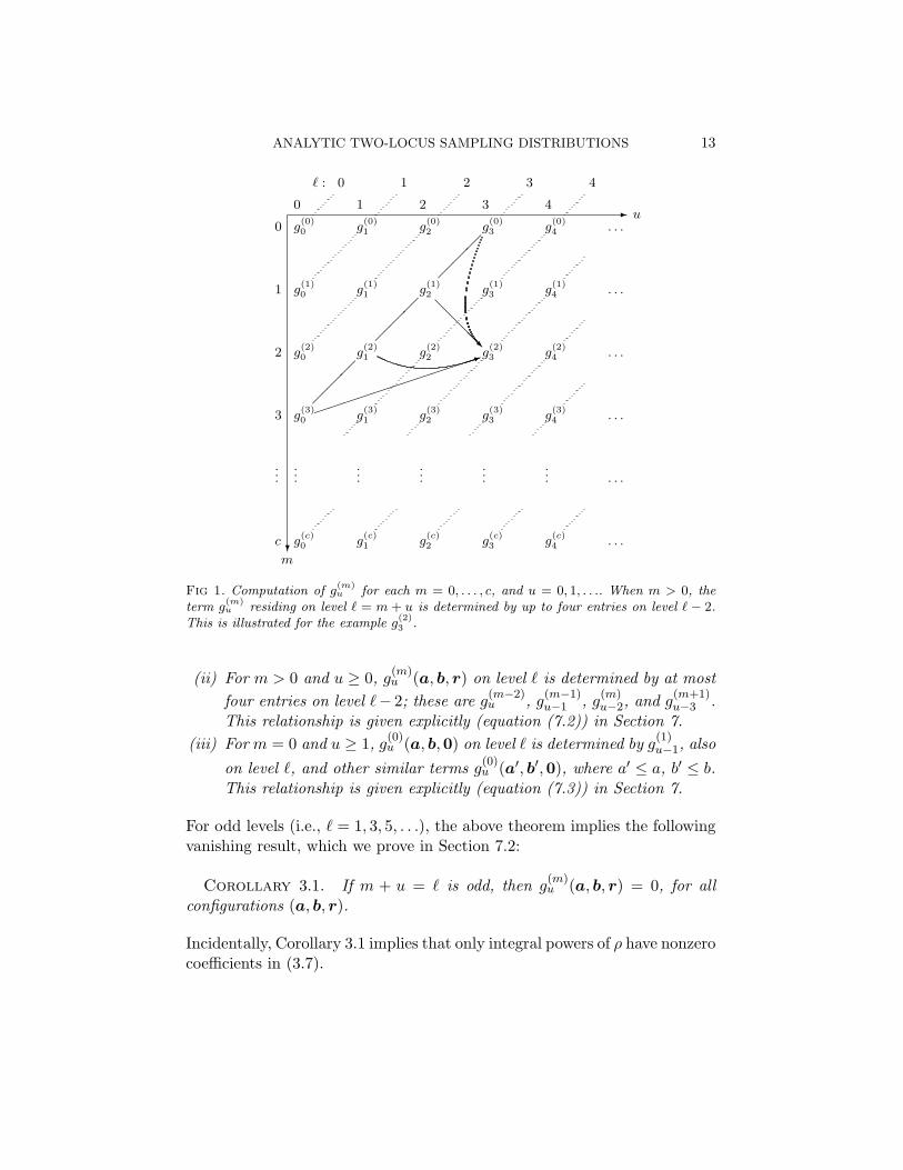
Fig 1. Computation of g(m)u for each m = 0, . . . , c, and u = 0, 1, . . .. When m > 0, the
term g(m)u residing on level ` = m + u is determined by up to four entries on level ` − 2.
This is illustrated for the example g(2)3 .
(ii) For m > 0 and u ≥ 0, g(m)u (a, b, r) on level ` is determined by at most
four entries on level `− 2; these are g(m−2)u , g
(m−1)u−1 , g
(m)u−2, and g
(m+1)u−3 .
This relationship is given explicitly (equation (7.2)) in Section 7.(iii) For m = 0 and u ≥ 1, g
(0)u (a, b,0) on level ` is determined by g
(1)u−1, also
on level `, and other similar terms g(0)u (a′, b′,0), where a′ ≤ a, b′ ≤ b.
This relationship is given explicitly (equation (7.3)) in Section 7.
For odd levels (i.e., ` = 1, 3, 5, . . .), the above theorem implies the followingvanishing result, which we prove in Section 7.2:
Corollary 3.1. If m + u = ` is odd, then g(m)u (a, b, r) = 0, for all
configurations (a, b, r).
Incidentally, Corollary 3.1 implies that only integral powers of ρ have nonzerocoefficients in (3.7).
14 P.A. JENKINS AND Y.S. SONG
Given the entries on level `− 2, Theorem 3.1 provides a method for com-puting each of the entries on level `. They can be computed in any order,apart from the slight complication of (iii), which requires knowledge of g
(1)u−1
as a prerequisite to g(0)u . The expression for g
(0)u (a, b,0) is only known re-
cursively in a and b, and we do not have a closed-form solution for thisrecursion for u ≥ 4 and even. Equation (2.10) provides one example, whichturns out to be the recursion for g
(0)4 (a, b,0). If the marginal one-locus sam-
pling distributions are known, the complexity of computing g(m)u (a, b, r) for
m > 0 does not depend on the sample configuration (a, b, r). In contrast, thecomplexity of computing g
(0)u (a, b,0) depends on a and b, and the running
time generally grows with sample size. However, in Section 6 we show thatignoring g
(0)u (a, b,0) generally leads to little loss of accuracy in practice.
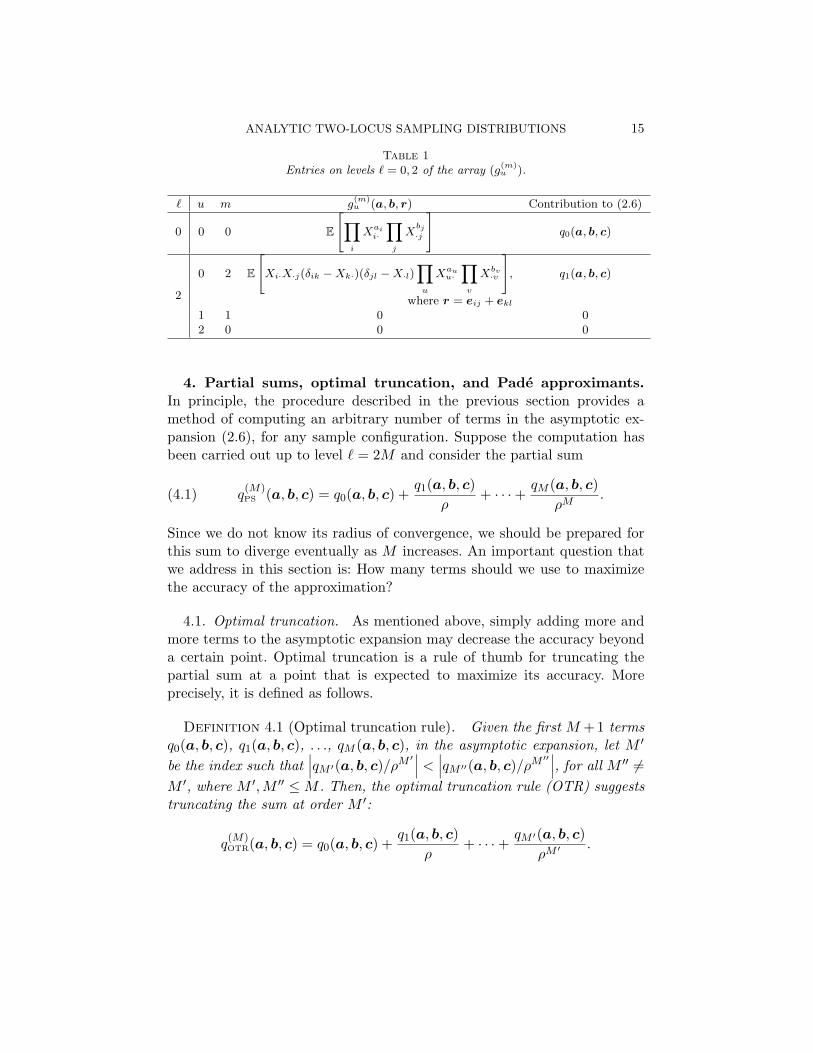
To illustrate the method, entries on the first two even levels are sum-marized in Table 1. These recapitulate part of the results given in Theo-rem 2.1. The last column of Table 1 gives the “contribution” to (2.6) fromg(m)u (a, b, r) (for fixed u and m and summing over the relevant r). According
to (3.7), this quantity is
(3.10)∑
r∈Pm
K∏i=1
L∏j=1
(cij
rij
) g(m)u (a + cA − rA, b + cB − rB, r).
We have also checked that the total contribution from entries on level ` = 4is equal to q2(a, b, c), as given in Theorem 2.1. We note in passing thatTheorem 3.1 makes it transparent why q2(a, b, c) is not universal in thesense described in Section 2.3: expressions on level ` = 4 depend directlyon L(0), which in turn depends upon the model of mutation. By contrast,the nonzero contribution to q1(a, b, c), for example, is determined by L(2),which does not depend on the model of mutation.
It is important to emphasize that g(m)u (a, b, r) is a function of the vec-
tors a, b, the matrix r, and (implicitly) the parameters θA and θB. Therelationships given in Theorem 3.1 are thus functional, and only need tobe computed once. In other words, all of these arguments of g
(m)u can re-
main arbitrary. It is not necessary to redo any of the algebraic computationsfor each particular choice of sample configuration, for example. Moreover,the solutions to each g
(m)u (a, b, r) are expressed concisely in terms of the
marginal one-locus sampling distributions qA and qB; this fact follows in-ductively from the solution for g
(0)0 (a, b,0). Unlike the method of Jenkins
and Song (2009, 2010), the iterative procedure here is essentially the sameat every step.
ANALYTIC TWO-LOCUS SAMPLING DISTRIBUTIONS 15
Table 1Entries on levels ` = 0, 2 of the array (g
(m)u ).
` u m g(m)u (a, b, r) Contribution to (2.6)
0 0 0 E
[∏i
Xaii·
∏j
Xbj
·j
]q0(a, b, c)
2
0 2 E
[Xi·X·j(δik −Xk·)(δjl −X·l)
∏u
Xauu·
∏v
Xbv·v
], q1(a, b, c)
where r = eij + ekl
1 1 0 02 0 0 0
4. Partial sums, optimal truncation, and Pade approximants.In principle, the procedure described in the previous section provides amethod of computing an arbitrary number of terms in the asymptotic ex-pansion (2.6), for any sample configuration. Suppose the computation hasbeen carried out up to level ` = 2M and consider the partial sum
(4.1) q(M)PS (a, b, c) = q0(a, b, c) +
q1(a, b, c)ρ
+ · · ·+ qM (a, b, c)ρM
.
Since we do not know its radius of convergence, we should be prepared forthis sum to diverge eventually as M increases. An important question thatwe address in this section is: How many terms should we use to maximizethe accuracy of the approximation?
4.1. Optimal truncation. As mentioned above, simply adding more andmore terms to the asymptotic expansion may decrease the accuracy beyonda certain point. Optimal truncation is a rule of thumb for truncating thepartial sum at a point that is expected to maximize its accuracy. Moreprecisely, it is defined as follows.
Definition 4.1 (Optimal truncation rule). Given the first M +1 termsq0(a, b, c), q1(a, b, c), . . ., qM (a, b, c), in the asymptotic expansion, let M ′
be the index such that∣∣∣qM ′(a, b, c)/ρM ′
∣∣∣ < ∣∣∣qM ′′(a, b, c)/ρM ′′∣∣∣, for all M ′′ 6=
M ′, where M ′,M ′′ ≤ M . Then, the optimal truncation rule (OTR) suggeststruncating the sum at order M ′:
q(M)OTR(a, b, c) = q0(a, b, c) +
q1(a, b, c)ρ
+ · · ·+ qM ′(a, b, c)ρM ′ .
16 P.A. JENKINS AND Y.S. SONG
The motivation for this rule is that the magnitude of the ith term in theexpansion is an estimate of the magnitude of the remainder. More sophisti-cated versions of the OTR are available (e.g. Dingle, 1973, Chapter XXI),but for simplicity we focus on the definition given above.
There are two issues with the OTR. First, it minimizes the error onlyapproximately, and so, despite its name, it is not be guaranteed to be op-timal. For example, the magnitude of the first few terms in the series canbehave very irregularly before a pattern emerges. Second, it may use onlythe first few terms in the expansion and discard the rest. As we discuss later,for some sample configurations and parameter values of interest, the OTRmight truncate very early, even as early as M ′ = 2. This is unrelated tothe first issue, since the series may indeed begin to diverge very early. Be-low, we discuss a better approximation scheme with a provable convergenceproperty.
4.2. Pade approximants. The key idea behind Pade approximants is toapproximate the function of interest by a rational function. In contrast tothe OTR, Pade approximants make use of all of the computed terms in theexpansion, even when the expansion diverges rapidly. More precisely, the[U/V ] Pade approximant of a function is defined as follows.
Definition 4.2 ([U/V ] Pade approximant). Given a function f andtwo nonnegative integers U and V , the [U/V ] Pade approximant of f is arational function of the form
[U/V ]f (x) =A0 + A1x + · · ·+ AUxU
B0 + B1x + · · ·+ BV xV,
such that B0 = 1 and
f(x)− [U/V ]f (x) = O(xU+V +1).
That is, the first U +V +1 terms in a Maclaurin series of the Pade approx-imant [U/V ]f (x) matches the first U + V + 1 terms in a Maclaurin seriesof f .
Our goal is to approximate the sampling distribution q(a, b, c) by thePade approximant
(4.2) q[U/V ]Pade (a, b, c) = [U/V ]q(a,b,c)
(1ρ
),
such that the first U + V + 1 terms in a Maclaurin series of [U/V ]q(a,b,c)(1ρ)
agrees with (4.1), where M = U + V . (In this notation, [U/V ]q(a,b,c)(1ρ) is
ANALYTIC TWO-LOCUS SAMPLING DISTRIBUTIONS 17
an implicit function of the mutation parameters.) As more terms in (4.1)are computed (i.e., as M increases), a sequence of Pade approximants canbe constructed. This sequence often has much better convergence propertiesthan (4.1) itself (Baker and Graves-Morris, 1996).
For a given M , there is still some freedom over the choice of U andV . As M increases, we construct the following “staircase” sequence of Padeapproximants: [0/0], [0/1], [1/1], [1/2], [2/2], . . .. This scheme is motivated bythe following lemma, proved in Section 7.3:
Lemma 4.1. Under a neutral, finite-alleles model, the sampling distribu-tion q(a, b, c) is a rational function of 1/ρ, and the degree of the numeratoris equal to the degree of the denominator.
This simple yet powerful observation immediately leads to a convergenceresult for the Pade approximants in the following manner:
Theorem 4.1. Consider a neutral, finite-alleles model. For every giventwo-locus sample configuration (a, b, c), there exists a finite nonnegative in-teger U0 such that for all U ≥ U0 and V ≥ U0, the Pade approximantq[U/V ]Pade (a, b, c) is exactly equal to q(a, b, c) for all ρ ≥ 0.
A proof of this theorem is provided in Section 7.4. Note that the staircasesequence is the “quickest” to reach the true sampling distribution q(a, b, c).Although Theorem 4.1 provides very strong information about the conver-gence of the Pade approximants, in practice U and V will have to be in-tractably large for such convergence to take place. The real value of Padesummation derives from the empirical observation that the approximantsexhibit high accuracy even before they hit the true sampling distribution.The staircase sequence also has the advantage that it exhibits a continuedfraction representation, which enables their construction to be made com-putationally more efficient (Baker and Graves-Morris, 1996, Chapter 4).
5. Incorporating selection. We now incorporate a model of diploidselection into the results of Section 3. Suppose that a diploid individual iscomposed of two haplotypes (i, j), (k, l) ∈ [K]×[L], and that, without loss ofgenerality, selective differences exist at locus A. We denote the fitness of thisindividual by 1 + sA
ik, and consider the diffusion limit in which σAik = 4NsA
ik
is held fixed for each i, k ∈ [K] as N →∞.In what follows, we use a subscript “s” to denote selectively nonneutral
versions of the quantities defined above. Results will be given in terms of thenonneutral one-locus sampling distribution qA
s at locus A and the neutralone-locus sampling distribution qB at locus B.
18 P.A. JENKINS AND Y.S. SONG
5.1. One-locus sampling distribution under selection. For the infinite-alleles model, one-locus sampling distributions under symmetric selectionhave been studied by Grote and Speed (2002), Handa (2005), and Huillet(2007). In the case of a parent-independent finite-alleles model, the station-ary distribution of the one-locus selection model is known to be a weightedDirichlet distribution (Wright, 1949):
πAs (x) = D
(K∏
i=1
xθAP A
i −1i
)exp
(12
K∑i=1
K∑k=1
σAikxixk
),
where x ∈ ∆K [see (2.1)] and D is a normalizing constant. The one-locussampling distribution at stationarity is then obtained by drawing a multi-nomial sample from this distribution:
(5.1) qAs (a) = Es
[K∏
i=1
Xaii
].
Thus, under a diploid selection model with parent-independent mutation,we are able to express the one-locus sampling distribution at least in inte-gral form. There are two integrals that need to be evaluated: one for theexpectation and the other for the normalizing constant. In practice, theseintegrals must be evaluated using numerical methods (Donnelly et al., 2001).
5.2. Two-locus sampling distribution with one locus under selection. Toincorporate selection into our framework, we first introduce some furthernotation.
Definition 5.1. Given two-locus population-wide allele frequencies x ∈∆K×L [see (2.3)], the mean fitness of the population at locus A is
σA(xA) =∑i,k
σAikxi·xk·.
Selection has an additive effect on the generator of the process, which isnow given by
Ls = L +12
∑i,j
xij
[∑k
σAikxk· − σA(xA)
]∂
∂xij,
where L is the generator (3.1) of the neutral diffusion process [see, forexample, Ethier and Nagylaki (1989)]. Rewriting Ls in terms of the LDvariables and then rescaling dij as before, we obtain
Ls = L +12
[ρL(2)
s +√
ρL(1)s + L(0)
s +1√
ρL(−1)
s
],
ANALYTIC TWO-LOCUS SAMPLING DISTRIBUTIONS 19
where L is as in (3.3), and the new contributions are
L(2)s = 0,
L(1)s = 0,
L(0)s =
∑i,j
dij
(∑k
σAikxk· − σA(xA)
)−∑k,k′
dkjσAkk′xi·xk′·
∂
∂dij
+∑
i
xi·
(∑k
σAikxk· − σA(xA)
)∂
∂xi·,
L(−1)s =
∑i,j,k
dijσAikxk·
∂
∂x·j.
In addition, we replace the asymptotic expansion (3.6) with
Es[G(m)(X;a, b, r)] = h(m)0 (a, b, r) +
h(m)1 (a, b, r)
√ρ
+h
(m)2 (a, b, r)
ρ+ · · · ,
the corresponding expansion for the expectation of G(m)(X;a, b, r) withrespect to the stationary distribution under selection at locus A. Finally,the boundary conditions (3.9) become the following (Fearnhead, 2003):
h(0)0 (ei,0,0) = φA
i , h(0)u (ei,0,0) = 0, ∀u ≥ 1,
h(0)0 (0, ej ,0) = πB
j , h(0)u (0, ej ,0) = 0, ∀u ≥ 1,(5.2)
h(0)0 (ei, ej ,0) = φA
i πBj , h(0)
u (ei, ej ,0) = 0, ∀u ≥ 1,
where φA = (φAi )i∈[K] is the stationary distribution for drawing a sample of
size one from a single selected locus.With only minor modifications to the arguments of Section 3, each term
in the array for h(m)u can be computed in a manner similar to Theorem 3.1.
In particular, entries on odd levels are still zero. Furthermore, as proved inSection 7.5, we can update Theorem 2.1 as follows:
Theorem 5.1. Suppose locus A is under selection, while locus B is se-lectively neutral. Then, in the asymptotic expansion (2.6) of the two-locussampling distribution, the zeroth and first order terms are given by (2.7) and(2.8), respectively, with qA
s (a) in place of qA(a). Furthermore, the second or-der term (2.9) may now be decomposed into two parts:
(5.3) q2,s(a, b, c) = q2,s(a + cA, b + cB,0) + σs(a, b, c),
20 P.A. JENKINS AND Y.S. SONG
where σs(a, b, c) is given by a known analytic expression and q2,s(a, b,0) sat-isfies a slightly modified version of the recursion relation (2.10) for q2(a, b,0).(These expressions are omitted for brevity.)
We remark that the above arguments can be modified to allow for locus Balso to be under selection, provided the selection is independent, with noepistatic interactions, and provided one can substitute φB
j for πBj in (5.2).
Then, one could also simply substitute qBs (b) for qB(b) in the expressions
for q0(a, b, c) and q1(a, b, c). However, for the boundary conditions (5.2) tobe modified in this way we would need to extend the result of Fearnhead(2003) to deal with two nonneutral loci, and we are unaware of such a resultin the literature.
6. Empirical study of accuracy. In this section, we study empiri-cally the accuracy of the approximate sampling distributions discussed inSection 4.
6.1. Computational details. As discussed earlier, a major advantage ofour technique is that, given the first M terms in the asymptotic expansion(2.6), the (M + 1)th term can be found and has to be computed only once.There are two complications to this statement: First, as mentioned in thediscussion following Theorem 3.1, the Mth order term qM for M ≥ 2 hasa contribution (namely, g
(0)2M (a, b,0)) that is not known in closed form, and
is only given recursively. (Recall that the M = 1 case is an exception, withg(0)2 (a, b,0) = 0 for all (a, b,0).) In Jenkins and Song (2009), it was ob-
served that the contribution of g(0)4 (a, b,0) to q2(a, b, c) is generally very
small, but that its burden in computational time increases with sample size.Extrapolating this observation to higher order terms, we consider makingthe following approximation:
Approximation 6.1. For all M ≥ 2, assume
g(0)2M (a, b,0) ≈ 0,
for all configurations (a, b,0).
As we show presently, adopting this approximation has little effect on theaccuracy of asymptotic sampling distributions. In what follows, we use thesymbol“ ” to indicate when the above approximation is employed. For ex-ample, the partial sum q
(M)PS (a, b, c) in (4.1) becomes q
(M)PS (a, b, c) under
Approximation 6.1.
ANALYTIC TWO-LOCUS SAMPLING DISTRIBUTIONS 21
Upon making the above approximation, it is then possible to construct aclosed-form expression for each subsequent term qM (a, b, c). However, thereis a second issue: Given the effort required to reach the complicated expres-sion for q2(a, b, c) (Jenkins and Song, 2009), performing the computationby hand for M > 2 does not seem tractable. Symbolic computation usingcomputer software such as Mathematica is a feasible option, but we deferthis for future work. Here, we are interested in comparing the accuracyof asymptotic sampling distributions with the true likelihood. Therefore, wehave implemented an automated numerical computation of each subsequentterm in the asymptotic expansion, for a given fixed sample configuration andfixed mutation parameters. For the samples investigated below, this did notimpose undue computational burden, even when repeating this procedureacross all samples of a given size. Exact numerical computation of the truelikelihood is possible for only small sample sizes (say, up to thirty), so werestrict our study to those cases.
For simplicity, we assume in our empirical study that all alleles are se-lectively neutral. Furthermore, we assume a symmetric, PIM model so thatP A = P B =
(1/2 1/21/2 1/2
), and take θA = θB = 0.01. This is a reasonable
approximation for modeling neutral single nucleotide polymorphism (SNP)data in humans (e.g. McVean et al., 2002). For the PIM model, recall thatthe marginal one-locus sampling distributions are available in closed-form,as shown in (2.5).
6.2. Rate of convergence: an example. To compare the convergence ofthe sequence of partial sums (4.1) with that of the sequence of Pade ap-proximants (4.2), we re-examine in detail an example studied previously.The sample configuration for this example is a = b = 0, c = ( 10 7
2 1 ). InJenkins and Song (2009), we were able to compute the first three termsin the asymptotic expansion, obtaining the partial sum q
(2)PS (a, b, c). Apply-
ing the new method described in this paper, we computed q(M)PS (a, b, c) for
M ≤ 11 (including the recursive terms g(0)u (a, b,0) discussed above), and
also the corresponding staircase Pade approximants q[U/V ]Pade (a, b, c). Results
are illustrated in Figure 2, in which we compare various approximations ofthe likelihood curve for ρ with the true likelihood curve. Here, the likelihoodof a sample is defined simply as its sampling distribution q(a, b, c) treatedas a function of ρ, with θA and θB fixed at 0.01.
Figure 2(a) exhibits a number of features which we also observed moregenerally for many other samples. For fixed ρ in the range illustrated, the se-quence (q(0)
PS , q(1)PS , q
(2)PS , . . .) of partial sums diverges eventually, and, for many
realistic choices of ρ, this divergence can be surprisingly early. Arguably
22 P.A. JENKINS AND Y.S. SONG
0 20 40 60 80 100
0
1
2
3
4
ρ
Lik
elih
oo
d (
10
−1
5)
0
1
2 3
4
5
6
7
8
9
10
11
0 2 3 100 2 10
(a)
0 20 40 60 80 1000
1
2
3
4
ρ
Lik
elih
oo
d (
10
−1
5)
[1/1]
[2/3]
[0/0]
(b)
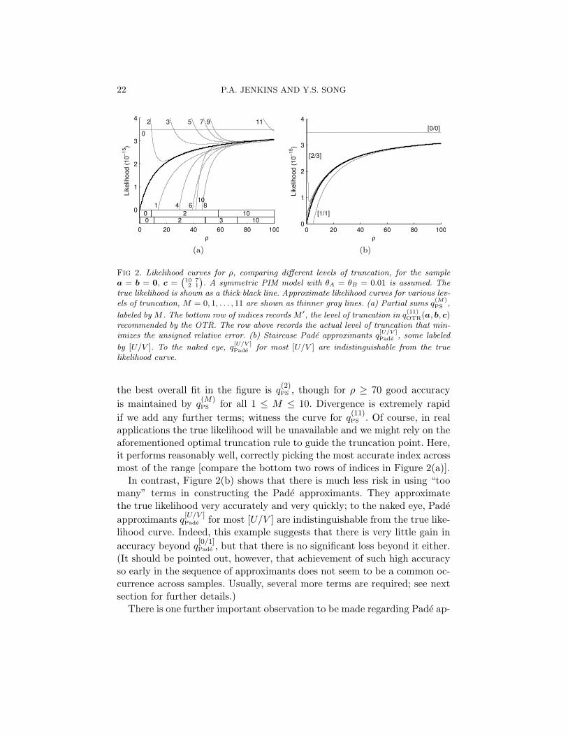
Fig 2. Likelihood curves for ρ, comparing different levels of truncation, for the samplea = b = 0, c =
(102
71
). A symmetric PIM model with θA = θB = 0.01 is assumed. The
true likelihood is shown as a thick black line. Approximate likelihood curves for various lev-els of truncation, M = 0, 1, . . . , 11 are shown as thinner gray lines. (a) Partial sums q
(M)PS ,
labeled by M . The bottom row of indices records M ′, the level of truncation in q(11)OTR(a, b, c)
recommended by the OTR. The row above records the actual level of truncation that min-imizes the unsigned relative error. (b) Staircase Pade approximants q
[U/V ]Pade , some labeled
by [U/V ]. To the naked eye, q[U/V ]Pade for most [U/V ] are indistinguishable from the true
likelihood curve.
the best overall fit in the figure is q(2)PS , though for ρ ≥ 70 good accuracy
is maintained by q(M)PS for all 1 ≤ M ≤ 10. Divergence is extremely rapid
if we add any further terms; witness the curve for q(11)PS . Of course, in real
applications the true likelihood will be unavailable and we might rely on theaforementioned optimal truncation rule to guide the truncation point. Here,it performs reasonably well, correctly picking the most accurate index acrossmost of the range [compare the bottom two rows of indices in Figure 2(a)].
In contrast, Figure 2(b) shows that there is much less risk in using “toomany” terms in constructing the Pade approximants. They approximatethe true likelihood very accurately and very quickly; to the naked eye, Padeapproximants q
[U/V ]Pade for most [U/V ] are indistinguishable from the true like-
lihood curve. Indeed, this example suggests that there is very little gain inaccuracy beyond q
[0/1]Pade , but that there is no significant loss beyond it either.
(It should be pointed out, however, that achievement of such high accuracyso early in the sequence of approximants does not seem to be a common oc-currence across samples. Usually, several more terms are required; see nextsection for further details.)
There is one further important observation to be made regarding Pade ap-
ANALYTIC TWO-LOCUS SAMPLING DISTRIBUTIONS 23
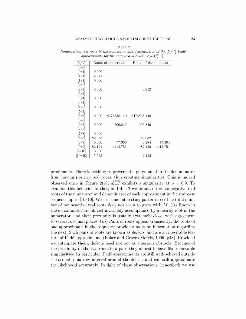
Table 2Nonnegative, real roots in the numerator and denominator of the [U/V ] Pade
approximants for the sample a = b = 0, c =(102
71
).
[U/V ] Roots of numerator Roots of denominator
[0/0][0/1] 0.000[1/1] 4.871[1/2] 0.000[2/2][2/3] 0.000 0.912[3/3][3/4] 0.000[4/4][4/5] 0.000[5/5][5/6] 0.000 8474538.140 8474538.140[6/6][6/7] 0.000 306.846 306.846[7/7][7/8] 0.000[8/8] 82.033 82.032[8/9] 0.000 77.366 0.284 77.364[9/9] 82.121 4412.751 82.120 4412.751[9/10] 0.000[10/10] 5.543 4.252
proximants. There is nothing to prevent the polynomial in the denominatorfrom having positive real roots, thus creating singularities. This is indeedobserved once in Figure 2(b); q
[2/3]Pade exhibits a singularity at ρ = 0.9. To
examine this behavior further, in Table 2 we tabulate the nonnegative realroots of the numerator and denominator of each approximant in the staircasesequence up to [10/10]. We see some interesting patterns: (i) The total num-ber of nonnegative real roots does not seem to grow with M . (ii) Roots inthe denominator are almost invariably accompanied by a nearby root in thenumerator, and their proximity is usually extremely close, with agreementto several decimal places. (iii) Pairs of roots appear transiently; the roots ofone approximant in the sequence provide almost no information regardingthe next. Such pairs of roots are known as defects, and are an inevitable fea-ture of Pade approximants (Baker and Graves-Morris, 1996, p48). Providedwe anticipate them, defects need not act as a serious obstacle. Because ofthe proximity of the two roots in a pair, they almost behave like removablesingularities. In particular, Pade approximants are still well-behaved outsidea reasonably narrow interval around the defect, and can still approximatethe likelihood accurately. In light of these observations, henceforth we use
24 P.A. JENKINS AND Y.S. SONG
the following simple heuristic for dealing with defects.
Definition 6.1 (Defect heuristic). Suppose we are interested in approx-imating the likelihood curve at a particular value ρ0 and have the resourcesto compute up to M in the partial sum (4.1). Then proceed as follows.
1. Initialize with M ′′ = M .2. Construct the [U/V ] Pade approximant in the staircase sequence, where
U + V = M ′′.3. If it exhibits a root in the interval (ρ0− ε, ρ0 + ε)∩ [0,∞), either in its
numerator or denominator, then decrement M ′′ by one and go to step2, otherwise use this approximant.
Choice of threshold ε involves a trade-off between the disruption causedby the nearby defect and the loss incurred by reverting to the previous Padeapproximant. Throughout the following section, we employ this heuristicwith ε = 25, which seemed to work well.
6.3. Rate of convergence: empirical study. To investigate to what extentthe observations of Section 6.2 hold across all samples, we performed thefollowing empirical study. Following Jenkins and Song (2009), we focusedon samples of the form (0,0, c) for which all alleles are observed at bothloci, and measured the accuracy of the partial sum (4.1) by the unsignedrelative error
e(M)PS (0,0, c) =
∣∣∣∣∣q(M)PS (0,0, c)− q(0,0, c)
q(0,0, c)
∣∣∣∣∣× 100%.
An analogous definition can be made for e(M)Pade, the unsigned relative error of
the staircase Pade approximants q[U/V ]Pade , where U = bM/2c and V = dM/2e.
When Approximation 6.1 is additionally used, the respective unsigned errorsare denoted e
(M)PS and e
(M)Pade. These quantities are implicit functions of the
parameters and of the sample configuration. In our study, we focused onsufficiently small sample sizes so that the true sampling distribution q(a, b, c)could be computed. Specifically, we computed q(0,0, c) for all samples ofa given size c using the method described in Jenkins and Song (2009). Byweighting samples according to their sampling probability, we may computethe distributions of e
(M)PS and e
(M)Pade, and similarly the distributions of e
(M)PS
and e(M)Pade. Table 3 summarizes the cumulative distributions of e
(M)PS and e
(M)Pade
for ρ = 50, across all samples of size c = 20 that are dimorphic at both loci.The corresponding table for e
(M)PS and e
(M)Pade was essentially identical (not

ANALYTIC TWO-LOCUS SAMPLING DISTRIBUTIONS 25
Table 3Cumulative distribution Φ(x) = P(e(M) < x%) (where e(M) denotes either e
(M)PS or e
(M)Pade)
of the unsigned relative error of the partial sum q(M)PS and the corresponding Pade
approximants, for all samples of size 20 dimorphic at both loci. Here, ρ = 50, andApproximation 6.1 is used.
TypeM of sum Φ(1) Φ(5) Φ(10) Φ(25) Φ(50) Φ(100)
0 PS 0.49† 0.56† 0.63 0.81 0.98 1.00Pade 0.49 0.56 0.63 0.81 0.98 1.00
1 PS 0.51 0.74 0.87 0.99 1.00 1.00Pade 0.59 0.77 0.84 0.91 0.98 0.99
2 PS 0.59 0.87 0.92 1.00 1.00 1.00Pade 0.77 0.97 0.98 0.99 1.00 1.00
3 PS 0.57 0.86 0.97 1.00 1.00 1.00Pade 0.91 0.96 0.98 0.99 1.00 1.00
4 PS 0.45 0.62 0.87 0.98 0.98 1.00Pade 0.95 0.99 1.00 1.00 1.00 1.00
5 PS 0.30 0.50 0.61 0.76 0.79 0.97Pade 0.98 1.00 1.00 1.00 1.00 1.00
10 PS 0.00 0.02 0.03 0.07 0.08 0.11Pade 1.00 1.00 1.00 1.00 1.00 1.00
OTR 0.25 0.36 0.65 0.89 0.90 1.00
† These two values were misquoted in the text of Jenkins and Song (2009, p. 1093); thistable corrects them.
shown), with agreement usually to two decimal places. This confirms thatutilizing Approximation 6.1 is justified.
Table 3 illustrates that the observations of Section 6.2 hold much moregenerally, as described below:
1. The error e(M)PS for partial sums is not a monotonically decreasing func-
tion of M ; i.e., the accuracy of q(M)PS improves as one adds more terms
up to a certain point, before quickly becoming very inaccurate.2. Empirically, the actual optimal truncation point for the parameter set-
tings we considered is at M ′ = 2 or M ′ = 3, which perform comparably.Moreover, both provide consistently higher accuracy than employingthe OTR, which is a serious issue when we wish to use this rule with-out external information about which truncation point really is themost accurate.
3. Overall, using Pade approximants is much more reliable. Note thatthe accuracy of Pade approximants continues to improve as we incor-porate more terms. For a sample drawn at random, the probabilitythat its Pade approximant is within 1% of the true sampling distribu-tion is 1.00, compared to 0.59 or 0.57 for truncating the partial sums
26 P.A. JENKINS AND Y.S. SONG
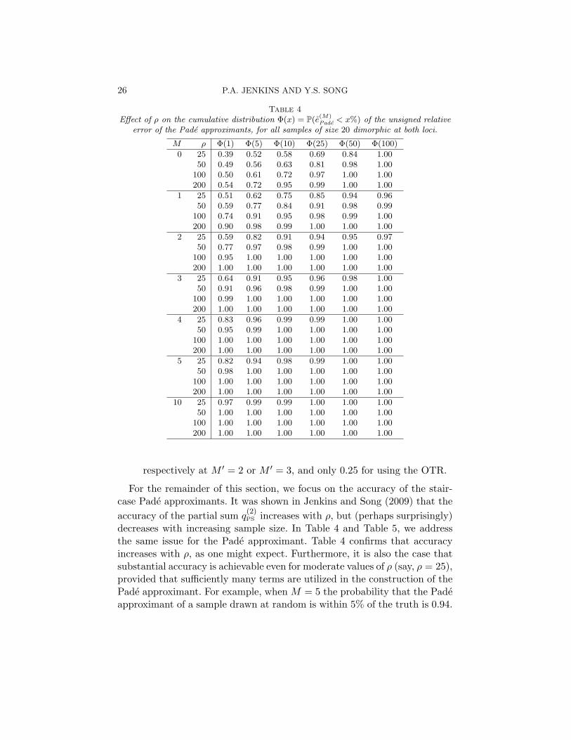
Table 4Effect of ρ on the cumulative distribution Φ(x) = P(e
(M)Pade < x%) of the unsigned relative
error of the Pade approximants, for all samples of size 20 dimorphic at both loci.
M ρ Φ(1) Φ(5) Φ(10) Φ(25) Φ(50) Φ(100)
0 25 0.39 0.52 0.58 0.69 0.84 1.0050 0.49 0.56 0.63 0.81 0.98 1.00
100 0.50 0.61 0.72 0.97 1.00 1.00200 0.54 0.72 0.95 0.99 1.00 1.00
1 25 0.51 0.62 0.75 0.85 0.94 0.9650 0.59 0.77 0.84 0.91 0.98 0.99
100 0.74 0.91 0.95 0.98 0.99 1.00200 0.90 0.98 0.99 1.00 1.00 1.00
2 25 0.59 0.82 0.91 0.94 0.95 0.9750 0.77 0.97 0.98 0.99 1.00 1.00
100 0.95 1.00 1.00 1.00 1.00 1.00200 1.00 1.00 1.00 1.00 1.00 1.00
3 25 0.64 0.91 0.95 0.96 0.98 1.0050 0.91 0.96 0.98 0.99 1.00 1.00
100 0.99 1.00 1.00 1.00 1.00 1.00200 1.00 1.00 1.00 1.00 1.00 1.00
4 25 0.83 0.96 0.99 0.99 1.00 1.0050 0.95 0.99 1.00 1.00 1.00 1.00
100 1.00 1.00 1.00 1.00 1.00 1.00200 1.00 1.00 1.00 1.00 1.00 1.00
5 25 0.82 0.94 0.98 0.99 1.00 1.0050 0.98 1.00 1.00 1.00 1.00 1.00
100 1.00 1.00 1.00 1.00 1.00 1.00200 1.00 1.00 1.00 1.00 1.00 1.00
10 25 0.97 0.99 0.99 1.00 1.00 1.0050 1.00 1.00 1.00 1.00 1.00 1.00
100 1.00 1.00 1.00 1.00 1.00 1.00200 1.00 1.00 1.00 1.00 1.00 1.00
respectively at M ′ = 2 or M ′ = 3, and only 0.25 for using the OTR.
For the remainder of this section, we focus on the accuracy of the stair-case Pade approximants. It was shown in Jenkins and Song (2009) that theaccuracy of the partial sum q
(2)PS increases with ρ, but (perhaps surprisingly)
decreases with increasing sample size. In Table 4 and Table 5, we addressthe same issue for the Pade approximant. Table 4 confirms that accuracyincreases with ρ, as one might expect. Furthermore, it is also the case thatsubstantial accuracy is achievable even for moderate values of ρ (say, ρ = 25),provided that sufficiently many terms are utilized in the construction of thePade approximant. For example, when M = 5 the probability that the Padeapproximant of a sample drawn at random is within 5% of the truth is 0.94.
ANALYTIC TWO-LOCUS SAMPLING DISTRIBUTIONS 27
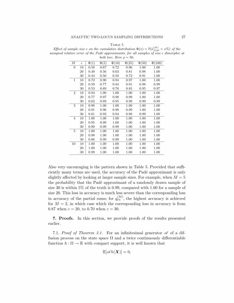
Table 5Effect of sample size c on the cumulative distribution Φ(x) = P(e
(M)Pade < x%) of the
unsigned relative error of the Pade approximants, for all samples of size c dimorphic atboth loci. Here ρ = 50.
M c Φ(1) Φ(5) Φ(10) Φ(25) Φ(50) Φ(100)
0 10 0.58 0.67 0.72 0.96 1.00 1.0020 0.49 0.56 0.63 0.81 0.98 1.0030 0.44 0.50 0.58 0.72 0.91 1.00
1 10 0.72 0.90 0.94 0.97 1.00 1.0020 0.59 0.77 0.84 0.91 0.98 0.9930 0.53 0.69 0.76 0.85 0.95 0.97
2 10 0.94 1.00 1.00 1.00 1.00 1.0020 0.77 0.97 0.98 0.99 1.00 1.0030 0.62 0.89 0.95 0.98 0.99 0.99
3 10 0.98 1.00 1.00 1.00 1.00 1.0020 0.91 0.96 0.98 0.99 1.00 1.0030 0.81 0.92 0.94 0.98 0.99 1.00
4 10 1.00 1.00 1.00 1.00 1.00 1.0020 0.95 0.99 1.00 1.00 1.00 1.0030 0.90 0.99 0.99 1.00 1.00 1.00
5 10 1.00 1.00 1.00 1.00 1.00 1.0020 0.98 1.00 1.00 1.00 1.00 1.0030 0.86 0.99 0.99 1.00 1.00 1.00
10 10 1.00 1.00 1.00 1.00 1.00 1.0020 1.00 1.00 1.00 1.00 1.00 1.0030 0.99 1.00 1.00 1.00 1.00 1.00
Also very encouraging is the pattern shown in Table 5. Provided that suffi-ciently many terms are used, the accuracy of the Pade approximant is onlyslightly affected by looking at larger sample sizes. For example, when M = 5the probability that the Pade approximant of a randomly drawn sample ofsize 30 is within 5% of the truth is 0.99, compared with 1.00 for a sample ofsize 20. This loss in accuracy is much less severe than the corresponding lossin accuracy of the partial sums; for q
(M)PS , the highest accuracy is achieved
for M = 2, in which case which the corresponding loss in accuracy is from0.87 when c = 20, to 0.70 when c = 30.
7. Proofs. In this section, we provide proofs of the results presentedearlier.
7.1. Proof of Theorem 3.1. For an infinitesimal generator A of a dif-fusion process on the state space Ω and a twice continuously differentiablefunction h : Ω → R with compact support, it is well known that
E[A h(X)] = 0,
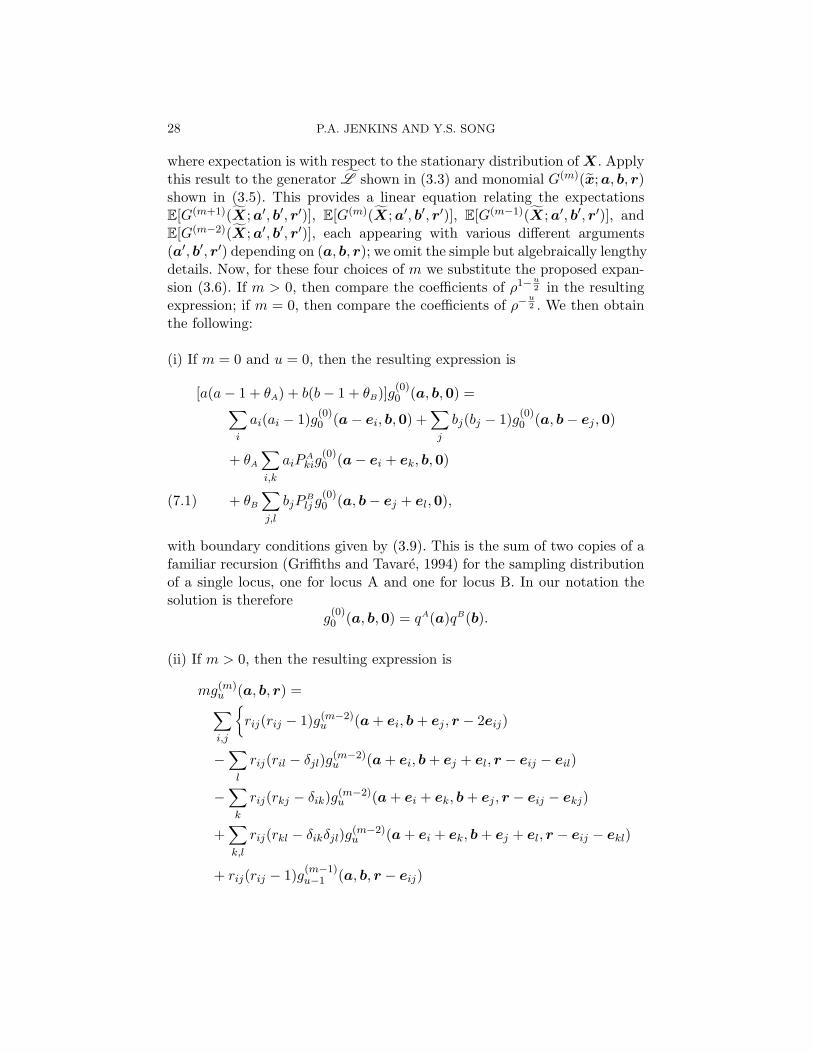
28 P.A. JENKINS AND Y.S. SONG
where expectation is with respect to the stationary distribution of X. Applythis result to the generator L shown in (3.3) and monomial G(m)(x;a, b, r)shown in (3.5). This provides a linear equation relating the expectationsE[G(m+1)(X;a′, b′, r′)], E[G(m)(X;a′, b′, r′)], E[G(m−1)(X;a′, b′, r′)], andE[G(m−2)(X;a′, b′, r′)], each appearing with various different arguments(a′, b′, r′) depending on (a, b, r); we omit the simple but algebraically lengthydetails. Now, for these four choices of m we substitute the proposed expan-sion (3.6). If m > 0, then compare the coefficients of ρ1−u
2 in the resultingexpression; if m = 0, then compare the coefficients of ρ−
u2 . We then obtain
the following:
(i) If m = 0 and u = 0, then the resulting expression is
[a(a− 1 + θA) + b(b− 1 + θB)]g(0)0 (a, b,0) =∑
i
ai(ai − 1)g(0)0 (a− ei, b,0) +
∑j
bj(bj − 1)g(0)0 (a, b− ej ,0)
+ θA
∑i,k
aiPAkig
(0)0 (a− ei + ek, b,0)
+ θB
∑j,l
bjPBlj g
(0)0 (a, b− ej + el,0),(7.1)
with boundary conditions given by (3.9). This is the sum of two copies of afamiliar recursion (Griffiths and Tavare, 1994) for the sampling distributionof a single locus, one for locus A and one for locus B. In our notation thesolution is therefore
g(0)0 (a, b,0) = qA(a)qB(b).
(ii) If m > 0, then the resulting expression is
mg(m)u (a, b, r) =∑i,j
rij(rij − 1)g(m−2)
u (a + ei, b + ej , r − 2eij)
−∑
l
rij(ril − δjl)g(m−2)u (a + ei, b + ej + el, r − eij − eil)
−∑k
rij(rkj − δik)g(m−2)u (a + ei + ek, b + ej , r − eij − ekj)
+∑k,l
rij(rkl − δikδjl)g(m−2)u (a + ei + ek, b + ej + el, r − eij − ekl)
+ rij(rij − 1)g(m−1)u−1 (a, b, r − eij)
ANALYTIC TWO-LOCUS SAMPLING DISTRIBUTIONS 29
− 2rij(ri· − 1)g(m−1)u−1 (a, b + ej , r − eij)
− 2rij(r·j − 1)g(m−1)u−1 (a + ei, b, r − eij)
+ 2∑k,l
rkj(ril − δikδjl)g(m−1)u−1 (a + ek, b + el, r − ekj − eil + eij)
+ 2(m− 1)rijg(m−1)u−1 (a + ei, b + ej , r − eij)
+∑
i
ai(ai + 2ri· − 1)g(m)u−2(a− ei, b, r)
+∑j
bj(bj + 2r·j − 1)g(m)u−2(a, b− ej , r)
− 2∑i,j
∑k
airkjg(m)u−2(a− ei + ek, b, r − ekj + eij)
− 2∑i,j
∑l
bjrilg(m)u−2(a, b− ej + el, r − eil + eij)
+ θA
∑i,k
P Aki
[aig
(m)u−2(a− ei + ek, b, r)
+∑j
rijg(m)u−2(a, b, r − eij + ekj)
]+ θB
∑j,l
P Blj
[bjg
(m)u−2(a, b− ej + el, r)
+∑
i
rijg(m)u−2(a, b, r − eij + eil)
]− [(a + m)(a + m + θA − 1) + (b + m)(b + m + θB − 1)
−m(m− 3)]g(m)u−2(a, b, r),
+ 2∑i,j
aibjg(m+1)u−3 (a− ei, b− ej , r + eij).(7.2)
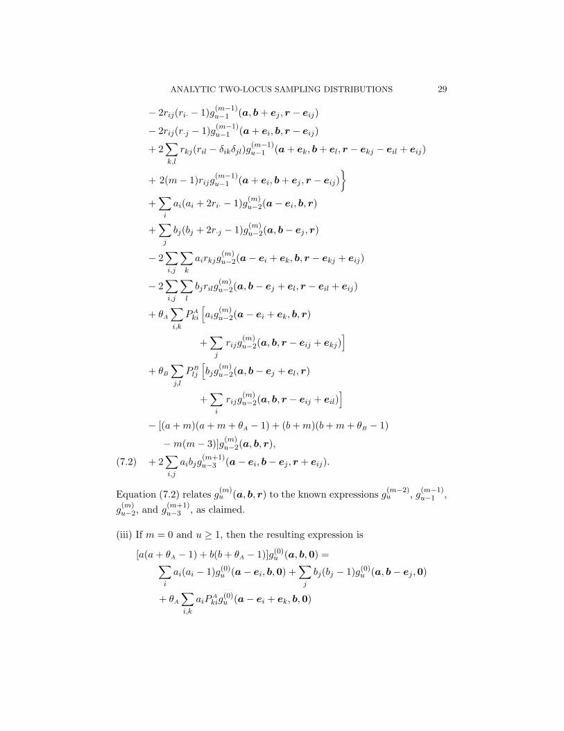
Equation (7.2) relates g(m)u (a, b, r) to the known expressions g
(m−2)u , g
(m−1)u−1 ,
g(m)u−2, and g
(m+1)u−3 , as claimed.
(iii) If m = 0 and u ≥ 1, then the resulting expression is
[a(a + θA − 1) + b(b + θA − 1)]g(0)u (a, b,0) =∑
i
ai(ai − 1)g(0)u (a− ei, b,0) +
∑j
bj(bj − 1)g(0)u (a, b− ej ,0)
+ θA
∑i,k
aiPAkig
(0)u (a− ei + ek, b,0)
30 P.A. JENKINS AND Y.S. SONG
+ θB
∑j,l
bjPBlj g(0)
u (a, b− ej + el,0)
+ 2∑i,j
aibjg(1)u−1(a− ei, b− ej , eij),(7.3)
with boundary conditions (3.9). Hence, this provides a recursion relation forg(0)u (a, b,0) when g
(1)u−1 is known.
7.2. Proof of Corollary 3.1. For the base case ` = 1, note that if m = 1and u = 0 then (7.2) simplifies to
g(1)0 (a, b, r) = 0,
and hence if m = 0 and u = 1 then (7.3) simplifies to
[a(a + θA − 1) + b(b + θA − 1)]g(0)1 (a, b,0) =∑
i
ai(ai − 1)g(0)1 (a− ei, b,0) +
∑j
bj(bj − 1)g(0)1 (a, b− ej ,0)
+ θA
∑i,k
aiPAkig
(0)1 (a− ei + ek, b,0)
+ θB
∑j,l
bjPBlj g
(0)1 (a, b− ej + el,0),(7.4)
with boundary conditions (3.9). This has solution
g(0)1 (a, b,0) = 0,
which is unique (since q(a, b, c) is unique). This completes ` = 1. Nowsuppose inductively that g
(m)u (a, b, r) = 0 for every m, u such that m + u =
`− 2 where ` is a fixed odd number greater than 1. Then for m, u such thatm + u = `, (7.2) becomes
g(m)u (a, b, r) = 0,
as required.
7.3. Proof of Lemma 4.1. In what follows, define the length of a sam-ple configuration (a, b, c) to be a + b + 2c. Under a neutral, finite-allelesmodel, the probability of a sample with length δ satisfies a closed system ofequations [e.g., see equation (5) of Jenkins and Song (2009)] which can beexpressed in matrix form:
Mq = v,
ANALYTIC TWO-LOCUS SAMPLING DISTRIBUTIONS 31
where q is a vector composed of the probabilities of samples of length lessthan or equal to δ, v is a constant vector of the same dimension as q, andM is an invertible matrix (since the solution to this equation is unique).The entries of M and v are rational functions of ρ, and hence q = M−1vis a vector each of whose entries is a rational function of ρ.
Let U0 denote the degree of the numerator, and V0 the degree of thedenominator. If U0 > V0, then q(a, b, c) becomes unbounded as ρ → ∞,while if V0 > U0 then q(a, b, c) → 0 as ρ →∞. But we know that q(a, b, c) isa probability, and hence bounded. Moreover, it has support over all samplesof a fixed size, since we assume that P A and P B are irreducible. Thus,to ensure limρ→∞ q(a, b, c) ∈ (0, 1) we must have U0 = V0. By a similarargument as ρ → 0, we must have that the coefficients of ρ0 are nonzeroboth in the numerator and in the denominator. We can therefore dividethe numerator and denominator by ρU0 to obtain a rational function of 1/ρwhose degree in the numerator and denominator are both U0 (= V0).
7.4. Proof of Theorem 4.1. This is an application of Theorem 1.4.4 ofBaker and Graves-Morris (1996), which we spell out for completeness. ByLemma 4.1, q(a, b, c) is a rational function of 1/ρ and is analytic at ρ = ∞with Taylor series (2.6). Denote the degree of its numerator and denominatorby U0. Then, q(a, b, c) has U0 + U0 + 1 independent coefficients determinedby the first U0 + U0 + 1 terms of its Taylor series expansion. Thus, providedU ≥ U0 and V ≥ U0, by the definition of the [U/V ] Pade approximant itmust coincide uniquely with q(a, b, c).
7.5. Proof of Theorem 5.1. This is simply an application of Theorem 3.1applied to the generator for the diffusion under selection, Ls, rather thanL , and so we just summarize the procedure.
The change in generator results in slight modifications to the relationshipsbetween the g
(m)u (a, b, r), in order to obtain the relationships between the
h(m)u (a, b, r) for each m and u:
1. h(0)0 (a, b,0) satisfies (7.1) (replacing each g
(0)0 with h
(0)0 ), but with extra
terms
+∑i,k
ai
[σikh
(0)0 (a + ek, b,0)−
∑k′
σAkk′h
(0)0 (a + ek + ek′ , b,0)
],
on the right-hand side. The solution is
h(0)0 (a, b,0) = qA
s (a)qB(b).
32 P.A. JENKINS AND Y.S. SONG
2. For m > 0, h(0)0 (a, b,0) satisfies (7.2) but with extra terms
(7.5) +∑i,k
(ai + ri·)σAikh
(m)u−2(a + ek, b, r)
− (a + m)∑k,k′
σAkk′h
(m)u−2(a + ek + ek′ , b, r)
−∑
i,j,k,k′
rijσAkk′h
(m)u−2(a + ei + ek, b, r − eij + ek′j)
on the right-hand side.3. For m = 0 and u ≥ 1, h
(0)0 (a, b,0) satisfies (7.2) but with extra terms
+∑i,k
[aiσ
Aikh
(0)u (a + ek, b,0)− aσA
ikh(0)u (a + ei + ek, b,0)
]+∑i,j,k
bjσAikh
(1)u−1(a + ek, b− ej , eij),
on the right-hand side.
Using these equations to evaluate h(m)u (a, b, r) on levels ` = 0, 1, . . . , 4 pro-
vides expressions for the nonneutral versions of q0(a, b, c), q1(a, b, c), andq2(a, b, c). Those for q0(a, b, c) and q1(a, b, c) in terms of the relevant one-locus sampling distributions are unchanged, while the new generator makessome minor modifications to the expression for q2(a, b, c). The analytic partof this term, σs(a, b, c), is easily calculated from h
(4)0 , h
(3)1 , h
(2)2 , and h
(1)3 ,
while the recursive part, q2,s(a + cA, b + cB,0) follows from h(0)4 .
Acknowledgments. We gratefully acknowledge Anand Bhaskar for im-plementing the algorithm stated in Theorem 3.1 and for checking some ofour formulas. We also thank Matthias Steinrucken and Paul Fearnhead foruseful discussion.
References.Baker, G. A. and Graves-Morris, P. Pade Approximants. Cambridge University Press,
2nd edition, 1996.Dingle, R. B. Asymptotic expansions: Their derivation and interpretation. Academic
Press, New York, 1973.Donnelly, P., Nordborg, M., and Joyce, P. (2001). Likelihoods and simulation methods for
a class of nonneutral population genetics models. Genetics, 159, 853–867.Ethier, S. N. (1979). A limit theorem for two-locus diffusion models in population genetics.
Journal of Applied Probability, 16, 402–408.Ethier, S. N. and Griffiths, R. C. (1990). On the two-locus sampling distribution. Journal
of Mathematical Biology, 29, 131–159.
ANALYTIC TWO-LOCUS SAMPLING DISTRIBUTIONS 33
Ethier, S. N. and Nagylaki, T. (1989). Diffusion approximations of the two-locus Wright-Fisher model. Journal of Mathematical Biology, 27, 17–28.
Ewens, W. J. (1972). The sampling theory of selectively neutral alleles. TheoreticalPopulation Biology, 3, 87–112.
Fearnhead, P. (2003). Haplotypes: the joint distribution of alleles at linked loci. Journalof Applied Probability, 40, 505–512.
Golding, G. B. (1984). The sampling distribution of linkage disequilibrium. Genetics,108, 257–274.
Griffiths, R. C. and Tavare, S. (1994). Simulating probability distributions in the coales-cent. Theoretical Population Biology, 46, 131–159.
Grote, M. and Speed, T. (2002). Approximate Ewens formulae for symmetric overdomi-nance selection. Annals of Applied Probability, 12, 637–663.
Handa, K. (2005). Sampling formulae for symmetric selection. Electronic Communicationsin Probability, 10, 223–234.
Hudson, R. R. (2001). Two-locus sampling distributions and their application. Genetics,159, 1805–1817.
Huillet, T. (2007). Ewens sampling formulae with and without selection. Journal ofComputational and Applied Mathematics, 206, 755–773.
Jenkins, P. A. and Song, Y. S. (2009). Closed-form two-locus sampling distributions:accuracy and universality. Genetics, 183, 1087–1103.
Jenkins, P. A. and Song, Y. S. (2010). An asymptotic sampling formula for the coalescentwith recombination. Annals of Applied Probability, 20, 1005–1028. (Technical Report775, Department of Statistics, University of California, Berkeley, 2009).
McVean, G., Awadalla, P., and Fearnhead, P. (2002). A coalescent-based method fordetecting and estimating recombination from gene sequences. Genetics, 160, 1231–1241.
McVean, G. A. T., Myers, S. R., Hunt, S., Deloukas, P., Bentley, D. R., and Donnelly, P.(2004). The fine-scale structure of recombination rate variation in the human genome.Science, 304, 581–584.
Ohta, T. and Kimura, M. (1969a). Linkage disequilibrium at steady state determined byrandom genetic drift and recurrent mutations. Genetics, 63, 229–238.
Ohta, T. and Kimura, M. (1969b). Linkage disequilibrium due to random genetic drift.Genetical Research, 13, 47–55.
Song, Y. S. and Song, J. S. (2007). Analytic computation of the expectation of the linkagedisequilibrium coefficient r2. Theoretical Population Biology, 71, 49–60.
Wright, S. Adaptation and selection. In Jepson, G. L., Mayr, E., and Simpson, G. G., edi-tors, Genetics, Paleontology and Evolution, pages 365–389. Princeton University Press,1949.
P. A. JenkinsComputer Science DivisionUniversity of California, BerkeleyBerkeley, CA 94720USAE-mail: [email protected]
Y. S. SongDepartment of Statistics and
Computer Science DivisionUniversity of California, BerkeleyBerkeley, CA 94720USAE-mail: [email protected]