on two flash methods for compositional reservoir...

1

On Two Flash Methods for Compositional Reservoir Simulations: Table

Look-up and Reduced Variables

Wei Yan*, Michael L. Michelsen, Erling H. Stenby, Abdelkrim Belkadi

Center for Energy Resources Engineering (CERE), Technical University of Denmark (DTU),

DK 2800, Kgs. Lyngby, Denmark

* Corresponding author, Tel.: +45 45252914, Fax: +45 45882258, E-mail: [email protected] Abstract

Compositional reservoir simulations are usually used for simulating enhanced oil

recovery processes involving large composition changes, such as gas injection. Phase

equilibrium calculation, which is often solved in terms of flash calculation, is the most

time consuming part in those simulations. Improving the flash calculation speed has

therefore become one of the central issues in compositional reservoir simulations, and

new algorithms for fast flash calculations are frequently proposed in the literature. Two

types of fast flash methods were recently investigated at DTU CERE, namely the

Compositional Space Adaptive Tabulation (CSAT) method and the reduced variables

methods. This paper summarizes the major results obtained in those studies.

CSAT is a table look-up method, which saves computation time by replacing rigorous

phase equilibrium calculations by the stored results in a tie-line table whenever the new

feed composition is on one of the stored tie-lines within a certain tolerance. With a

slimtube simulator, it has been investigated whether the table look-up method can

compete with an efficient implementation of phase split calculation in two-phase regions.

The number of tie-lines stored for comparison and the tolerance set for accepting the feed

composition greatly influence the simulation speed and the accuracy of simulation results.

An important observation is that the table look-up itself is not free and its cost can be

comparable to the efforts for a rigorous flash. An alternative method, the Tie-line

Distance Based Approximation (TDBA) method, was proposed to get the approximate

results without performing a table look-up. TDBA can cut the simulation time by half or

even higher for the tests with cubic EoS’s. It has a bigger potential for speeding up

simulations with more advanced and complicated EoS’s.

2

The reduced variables methods or the reduction methods reformulate the original phase

equilibrium problem with a smaller set of independent variables. Various versions of the

reduced variables have been proposed since the late 80’s while efficiency of the methods

was recently questioned by Haugen and Beckner (2011). With the recent formulations by

Nichita and Garcia (2010), it is possible to code the reduced variables methods without

extensive modifications of Michelsen’s conventional flash algorithm. A simple test using

the SPE 3 example was performed, showing that the best reduction in time was less than

20% for the extreme situation of 25 components and just one row/column with non-zero

binary interaction parameters. A better performance can be achieved by a simpler

implementation using the sparsity of the interaction parameter matrix.

1. Introduction

Equation of State (EoS) based compositional reservoir simulations are usually employed

when the composition effects can no longer be accounted for by a black oil model. In

compositional reservoir simulations, solution to the phase equilibrium equations is often

separated from solution to the transport equations. In that case, the phase equilibrium

equations are solved by the so called flash algorithm, where the phase amounts and the

equilibrium phase compositions are computed for a given feed composition at specified

temperature and pressure. The calculation algorithm for two-phase isothermal flash is

rather matured (Michelsen, 1982a and 1982b; Michelsen and Mollerup, 2007) and the

solution procedure consists of two steps, a stability analysis step to determine whether the

feed will split into two phases, and a phase split step to calculate the equilibrium

compositions using the initial estimates from the first step. The algorithm is proposed for

general situations where there is not a priori information about the possible results. It

stresses more on safety than on speed. However, speed is a crucial concern in

compositional reservoir simulations since flash calculation with a complicated EoS model

increases the computation time dramatically. Speeding up the flash calculation without

too much compromise in accuracy and reliability has always been a research topic in

compositional reservoir simulations.

3

The computation time spent on flash calculations can be reduced by different strategies.

One recent effort is the shadow region method (Rasmussen et al., 2006; Michelsen and

Mollerup, 2007) which reduces the computation time mainly by skipping stability

analysis for a large portion of compositions in the single phase region. In the two-phase

region, a highly efficient Newton-Raphson algorithm can be employed with initial

estimates from the previous step. The shadow region method has been applied to

compositional transient pipeline simulations (Rasmussen et al., 2006). Another recent

effort is represented by the Compositional Space Parameterization (CSP) framework and

the Compositional Space Tabulation (CST) method (Voskov and Tchelepi, 2007, 2008a

and 2008b), which is based on CSP. In the CST method, a table of converged flash

calculations (tie-lines) is built to parameterize the compositional space. The table can be

updated adaptively and the corresponding method is known as the Compositional Space

Adaptive Tabulation (CSAT) method. During a simulation run with CSAT, it is checked

if the feed composition lies on one of the stored tie-lines within a certain tolerance. The

standard EoS-based phase equilibrium calculation will be replaced if a stored tie-line is

identified in the tie-line table look-up. This look-up strategy can be applied to replace

both stability analysis and phase split (Voskov and Tchelepi, 2007, 2008a and 2008b).

The CSAT method has been implemented to a General Purpose Research Simulator

(GPRS) for simulating multicomponent immiscible, and miscible gas injection scenarios

(Voskov and Tchelepi, 2007, 2008a and 2008b). It is reported that the CSAT strategy can

lead to significant gains in computational efficiency compared to standard EoS based

compositional simulation (Voskov and Tchelepi, 2009) The authors also showed that the

adaptive tabulation approach can be extended to systems with component that partition

among three, or more, fluid phase equilibrium (Voskov and Tchelepi, 2009). Another

way of reducing the flash calculation time is through the reduced variables methods

(Michelsen, 1986; Hendriks, 1988; Firoozabadi and Pan, 2002; Pan and Firoozabadi,

2003). The reduced variables methods take advantage of the form of cubic equations of

state and approximate the original set of equations by a smaller set of equations.

This paper is based on two recent studies carried out at Center for Energy Resources

Engineering (CERE), DTU (Belkadi et al., 2011; Michelsen, 2011). The first part in this

4

paper is about the table loop-up approach (Belkadi et al., 2011) and the second part is

about the reduced variables method (Michelsen, 2011). The purpose is to compare those

methods with the existing fast flash or conventional flash methods.

2. Table look-up methods

In the study of the table look-up methods, we use the shadow region method as the basis

for a fast flash calculation strategy. The method provides a simple but reliable way to

skip stability analysis in single phase regions, and no compromise in accuracy in two-

phase regions. We also notice that the tie-line table look-up technique employed by

CSAT has the potential to further reduce the computation time in the two-phase region by

approximating the rigorous phase split results with the results of an existing tie-line. The

approximation in the two-phase region has been implemented in two different ways: the

Tie-line Table Look-up (TTL) approach, which is similar to CSAT, and the tie-line

distance based approximation (TDBA) approach, which is improved based on the

analysis of the first one. In the following subsections, a brief description of the shadow

region will be given first. Then, the TTL methods and the TDBA methods will be

introduced. Finally, several 1-D multicomponent gas injection problems will be used to

compare the TTL method and the TDBA method with the shadow region method as

reference.

2.1. Shadow region method

The shadow region method takes advantage of the previous results to speed up flash

calculations (Rasmussen et al., 2006; Michelsen and Mollerup, 2007). For a given feed

composition, the shadow region refers to the part in the single phase region where a non-

trivial positive minimum of the tangent plane distance exists. The flash results of a feed

composition in a previous time step may fall into three different regions: the two-phase

region, the shadow region (single phase), and outside the shadow region (single phase).

Depending on which region it is, the flash strategies for the new feed composition in the

same grid block is different. In the two-phase region, a second order Newton-Raphson

algorithm is directly used with initial estimates given by

5

,i i new iv z , 1i i new il z (1)

with the vapor split factors defined by

1i

ii i old

y

y x

(2)

If it does not converge, the calculation procedure is reverted to the safe traditional flash

procedure (Michelsen and Mollerup, 2007). In the shadow region, the non-trivial solution

from the previous tangent plane distance minimization is stored as the shadow phase. Its

composition is used as initial estimates for the stability analysis of the new composition.

Different from the traditional flash procedure, only one-sided stability analysis starting

from a second-order minimization is needed here. For a feed composition outside the

shadow region, if it is not too close to the critical point, it is safe to assume the new flash

results will be still in the single phase region and stability analysis can therefore be

skipped. If the composition is close to the critical point, the safe flash approach with

stability analysis must be employed. Rasmussen et al. (2006) suggested using the

minimum eigenvalue, λ1 of the Hessian matrix H used in minimizing tangent plane

distance, as such a measure of the closeness to the critical point. If the changes in

composition, pressure, and temperature satisfy the following criteria

, 10.1i i oldz z , 10.1oldP P P , 110 (K)oldT T (3)

we skip stability analysis.

2.2. Tie-line Table Look-up (TTL)

The TTL methods were modified from the CSAT method (Voskov and Tchelepi, 2007,

2008a and 2008b). CSAT was inspired by the special feature in the analytical solution of

1-D gas injection processes that the 1-D analytical solution usually contains just a limited

number of tie-lines (Orr, 2007). It is argued that a table without too many representative

tie-lines can provide good approximation for the injection simulation. Although CSAT is

based on 1-D gas injection processes, it can be applied to speeding up phase equilibrium

calculations in general compositional reservoir simulations.

6

CSAT relies on building up a table of tie-lines and comparing the new feed composition

with the existing tie lines (Voskov and Tchelepi, 2007, 2008a and 2008b). To check if the

composition lies on one of the stored tie-lines or its extension, the following equations are

used

kj j

k kj j

z x

y x

(4)

2( (1 ) )k k

i i ii

z y x (5)

Here, the component j can be arbitrarily chosen. β is the vapor fraction, zi denotes the

mole fractions of component i in the new feed. kjx and k

jy represent the mole fractions in

the liquid and vapor phases for tie-line k. If one of the stored tie-lines satisfies the above

criteria, it is possible to skip the EoS-based phase equilibrium calculation. Otherwise, a

standard flash calculation is used to calculate the results and generate a new tie-line. The

tie-line table is constructed in advance and updated during the simulation. For simulations

not at a constant pressure, tie-line tables at several pressures must be constructed for

pressure interpolation during the simulation.

The TTL method is formulated in a way different from CSAT. Instead of using Eqs. (5)

and (6) to calculate the distance from the new feed composition to an existing tie-line, it

is suggested that the shortest distance between the feed and tie-line k should be calculated

(Michelsen, 2010). If we denote the shortest distance to tie-line k by dk. (dk)2 or the

minimum error ek can be obtained by the following minimization

2

min 1k k ki i i

i

e z y x (6)

The vapor fraction from the minimization is given by

Tk k k

Tk k k k

z x y x

y x y x (7)

In Eqs.(4) and (5), is arbitrarily calculated and there are Nc possible distances to a tie-

line for a Nc component system. The new formulation by Eqs. (6) and (7) gives a unique

distance to tie-line k (hereafter called tie-line distance) and the calculation is also direct.

7

For a new feed composition in the two-phase region, we calculate its shortest distance to

tie-line k using Eqs. (6) and (7). If ek<ε, we accept the tie-line as flash solution; if ek>ε

for all the M tie-lines in the table, we flash the new composition, and in the case of two

phases, we include the solution in the tie-line set. The TTL method is only applied in the

two-phase region to speed up the calculation by approximating the rigorous results with

existing tie-lines. In the single phase region, the shadow region criteria are used to judge

whether stability analysis can be skipped.

2.3. Tie-line Distance Based Approximation (TDBA)

Instead of building a tie-line table for comparison, a simple way is suggested to find a

neighboring tie-line and to utilize its information to approximate flash results (Michelsen,

2010). For a new composition in a given grid block, it is assumed that the tie-line from

the previous rigorous flash calculation can be a good approximation to the new flash. No

tie-line table is constructed here. The distance between the new composition and the tie-

line from the previous flash calculation is calculated using Eqs. (6) and (7). Since there is

only one tie-line for comparison, only one distance (or error), e, needs to be calculated.

The flash is then proceeded in three different ways depending on the magnitude of e:

if e > ε, we do new flash;

if ε > e > 10-4ε, we use old results but adjustment is needed;

if e < 10-4ε, we use the previous results as a solution without any adjustment.

Since the method uses the distance to a tie-line to judge whether we can make

approximation to the rigorous flash results, we hereafter call it Tie-line Distance Based

Approximation (TDBA). It should be noted that when e is in the intermediate range (ε > e

> 10-4ε), we can either solve the Rachford-Rice equation with the old K-values or directly

adjust the material balance using Eqs. (1) and (2). These two options are denoted by

TDBA1 and TDBA2, respectively.

8

2.4. Results and Discussion

A one-dimensional slimtube simulator was used here to test different methods.

Description about the slimtube simulator can be found in Michelsen (1998) and Yan et al.

(2004). The shadow region criteria were used in single-phase regions to skip stability

analysis. In the two-phase region, the TTL and the TDBA options were implemented to

study their computational performance as compared with the efficient implementation of

direct Newton-Raphson method originally employed in the slimtube simulator. The

option of using direct Netwon-Rapshon method is termed as the shadow region method

here. It serves as a reference option to compare with the other two options: TTL and

TDBA. Another reference option used in the computation speed comparison is the full

stability analysis method, where full stability analysis is performed whenever a flash

calculation is made. The full stability analysis method is much slower than the shadow

region method, whereas both methods make no approximations in phase equilibrium

solutions.

Four gas injection systems have been studied here (Table 1): System 1 is a 13-component

system, with detailed fluid description given in Table 2; Systems 2 to 4 correspond to the

systems studied by Zick (1986). The fluid description for Systems 2 to 4, listed in Table

3, is originally created by Jessen (2000). The experimental MMPs for Systems 2 to 4 are

150, 220, and 240 atm, respectively (Zick, 1986). Jessen’s description predicts similar

MMP values. Soave-Redlich-Kwong (SRK) EoS (Soave 1972) is used for System 1 and

Peng-Robinson (PR) EoS (Peng and Robinson 1976) is used for Systems 2 to 4.

Table 1. Overview of the four gas injection systems

System 1 System 2 System 3 System 4

Oil 13-component oil Zick Oil 1 Zick Oil 2 Zick Oil 3

Gas 0.8 CO2+ 0.2 C1 Zick Gas 1 Zick Gas 2 Zick Gas 3

T (K) 375.00 358.15 358.15 358.15

p (atm) 300 140 200 230

EoS used SRK PR PR PR

9

Table 2. Fluid description for gas injection system 1

zoil zgas Tc (K) pc (atm) ω MW (g/mol) kCO2,j

CO2 0.003699 0.8 304.2 72.8 0.225 44.01 0.00

C1 0.435813 0.2 190.6 45.4 0.008 16.04 0.12

C2 0.074085 305.4 48.2 0.098 30.07 0.12

C3 0.062088 369.8 41.9 0.152 44.09 0.12

i-C4 0.010398 408.1 36.0 0.176 58.12 0.12

C4 0.031394 425.2 37.5 0.193 58.12 0.12

i-C5 0.011498 460.4 33.4 0.227 72.15 0.12

C5 0.016497 469.6 33.3 0.251 72.15 0.12

C6 0.022396 507.4 29.3 0.296 86.17 0.12

C7 0.034293 529.5 32.3 0.4591 100.20 0.10

C8 0.040692 547.1 30.4 0.4854 114.23 0.10

C9 0.025295 568.1 27.4 0.5228 128.25 0.10

C22 0.228254 810.3 15.1 1.0315 310.60 0.10

Table 3. Fluid description for gas injection systems 2 to 4 (Zick oils and gases) zoil1

zoil2

zoil3

zgas1

zgas2

zgas3

Tc (K)

pc (atm)

ω

MW (g/mol)

kCO2,j

CO2 0.0483 0.0652 0.0673 0.2218 0.1774 0.1708 304.2 72.9 0.228 44.01 0

C1 0.2067 0.3542 0.3792 0.2349 0.3879 0.4109 190.6 45.4 0.008 16.04 0.105

C2 0.048 0.0534 0.0537 0.235 0.188 0.181 305.4 48.2 0.098 30.07 0.130

C3 0.0408 0.0377 0.037 0.2745 0.2196 0.2114 369.8 41.9 0.152 44.09 0.125

C4 0.0322 0.0266 0.0257 0.0338 0.027 0.0208 425.2 37.5 0.193 58.12 0.115

C5 0.0246 0.0192 0.0184 469.6 33.3 0.251 72.15 0.115

C6 0.0296 0.0225 0.0214 507.4 29.3 0.296 86.17 0.115

C7+(1) 0.2515 0.1859 0.1755 616.2 28.5 0.454 137.69 0.115

C7+(2) 0.128 0.0946 0.0891 698.9 19.1 0.787 243.95 0.115

C7+(3) 0.0851 0.0629 0.0593 770.4 16.4 1.048 347.69 0.115

C7+(4) 0.0629 0.0465 0.0438 853.1 15.1 1.276 481.03 0.115

C7+(5) 0.0425 0.0315 0.0296 1001.2 14.5 1.299 735.68 0.115

In all the simulations, a simple relative permeability model is used where the relative

permeability for a specific phase is set to the square of its saturation. A fixed viscosity

ratio between oil and gas (5:1) is used. All the simulations have used an implicit single-

point upstream scheme with 500 grid blocks. The time step is set to Δt/Δx =0.1 unless

otherwise mentioned. All experiments were run on an Intel Core™ Duo CPU with 3 GHz

processor and 1.94 GB of RAM.

10

First, System 1 is used to analyze the performance of the TTL method. For TTL with the

tie-line table generated and updated during the simulation, its performance is influenced

by the tolerance used and the maximum number of tie-lines allowed in the tie-line table,

M. During the calculation, a new tie-line is stored whenever a new set of two-phase

results is obtained from the rigorous flash calculation. The time used in comparing with

the stored tie-lines and managing the tie-line table will increase with the number of tie-

lines in the table. In principle, sorting the tie-lines can move the most hit tie-lines to the

top of the table and thus reduces the searching time. However, sorting itself is also time-

consuming. We found that a partial sorting, i.e., simply moving a tie-line forward if its

number of hits is higher than that of the neighboring tie-line just before it, only reduces

the simulation time obviously if a larger number of tie-lines are used. But the simulation

time in that case is usually too long, which makes the method unattractive.

Table 4 - Performance of TTL method for System 1 with PVI=0.5 and different M and ε and time step.

ε =10-4 ε =10-5 ε =10-6 ε =10-7 M = 100 Time (sec) 4.2 7.0 7.1 7.1

% skips 41% 0.1% 0.0% 0.0% Ntieline 100 100 100 100

M = 500 Time (sec) 2.0 18.1 21.2 21.5 % skips 99.9% 10% 0.3% 0.2% Ntieline 482 500 500 500

M = 1000 Time (sec) 2.0 28.8 37.3 38.3 % skips 99.9% 18% 0.9% 0.4% Ntieline 482 1000 1000 1000

M = 5000 Time (sec) 2.0 66.4 134.8 157.2 % skips 99.9% 64.7% 25.8% 7% Ntieline 482 5000 5000 5000

Table 4 shows the TTL results for System 1 with PVI=0.5. The simulation time is

strongly influenced by the maximum number of tie-lines, M. In general, the actual

number of tie-lines used during the simulation, Ntieline, increases with M. More tie-lines

will increase the time used in managing the tie-lines and the overall simulation time also

increases. For ε = 10-4, Ntieline does not increase with M, and the change in simulation time

does not follow the aforementioned trend. Besides, the simulation results are not accurate

at big tolerances. At ε = 10-4, none of the simulation results are acceptable. Figure 1

provides an example at M=1000. Compared to the accurate gas saturation profile, i.e., the

profile from the full stability analysis method or the shadow region method, where no

approximation is made in flash solutions, the TTL results are unacceptable at ε = 10-4 and

11

10-5. At ε = 10-6 and 10-7 for M=1000, the CSAT results are closer to the accurate

solution, but the number of approximations (% skips) are actually very small. For higher

M, the tolerance that can give an acceptable solution becomes even smaller. Although the

number of skips will increase, the simulation time becomes too long and even longer than

doing full stability analysis for all the flashes.

0

0,2

0,4

0,6

0,8

1

0 100 200 300 400 500

Gas Saturation

Cell Number

Accurate solution

TTL, M=1000 eps=1E-4




0

0,2

0,4

0,6

0,8

1

0 100 200 300 400 500

Gas Saturation

Cell Number

Accurate solution





(a) (b)

Figure 1. Gas saturation profile for System 1 at 0.5 PVI by TTL method a) Δt/Δx =0.1 b) Δt/Δx =0.5.

0

0,2

0,4

0,6

0,8

1

0 100 200 300 400 500

Gas Saturation

Cell Number

Accurate solution

TTL-PRE, eps=1E-4

TTL-PRE, eps=1E-5

TTL-PRE, eps=1E-6

TTL-PRE, eps=1E-7

0

0,2

0,4

0,6

0,8

1

0 100 200 300 400 500

Gas Saturation

Cell Number

Accurate solution

TTL-PRE, eps=1E-4

TTL-PRE, eps=1E-5

TTL-PRE, eps=1E-6

TTL-PRE, eps=1E-7

(a) (b) Figure 2. Gas saturation profile for System 1 at 0.5 PVI by TTL-PRE method a) Δt/Δx =0.1 b) Δt/Δx

=0.5.

12

0

10

20

30

40

50

60

70

80

90

100

0 0,2 0,4 0,6 0,8 1 1,2 1,4 1,6 1,8 2

Recovery (%)

PVI

Accurate solution

TTL-PRE, eps=1E-4

TTL-PRE, eps=1E-5

TTL-PRE, eps=1E-6

TTL-PRE, eps=1E-7

Figure 3. Oil recoveries for System 1 by TTL-PRE method.

Using a pre-calculated tie-line table can dramatically cut the time in managing tie-lines.

We used M = 20000 and ε = 10-8 to find the most frequently used tie-lines during the

simulation. Three tie-lines were identified, which account for 27%, 36% and 25% of the

total tie-line usage. These three tie-lines were used to construct a fixed tie-line table

which is used throughout the simulation. This variation is referred to as TTL-PRE. Figure

2 shows the results for TTL-PRE, the results are generally better than TTL but still not

satisfactory. There is always some discrepancy between the TTL-PRE solution and the

accurate solution. For smaller ε, the simulation time gets closer to that for the shadow

region method where no approximation is made. Figure 3 shows the recovery curves

calculated by TTL-PRE using different ε. All the tolerances except ε = 10-4 give almost

the same recovery as the accurate solution, despite the discrepancy observed in Figure 2.

Table 5 compares the simulation times used for different methods for System 1 and

provides details on how flash calculations are approximated in TTL, TTL-PRE, TDBA1

and TDBA2. Calculation with full stability analysis is given as a reference. The shadow

region method is around 15 times faster than the full stability analysis method. Table 5

only provides the TTL with acceptable gas saturation profiles (although for M = 5000, ε =

10-7, there is still some discrepancy). Their simulation times are actually longer than that

for the shadow region method. This is because that very few percentages of

approximation have been made and a lot of time is spent on tie-line management. TTL-

PRE is much faster than TTL and for ε = 10-4 to 10-6, it is also faster than the shadow

region method. However, as Figure 2 indicates, the TTL-PRE solution is not satisfactory

13

for those tolerances. At ε = 10-7, there is no significant difference in simulation time

between the TTL-PRE method and the shadow region method. Among all the methods,

TDBA1 and TDBA2 are the fastest. Their simulation times can be 1/3 to 2/3 shorter than

that for the shadow region method, depending on PVI and ε. TDBA1 and TDBA2 show

almost the same performance in terms of simulation time and percentage of skips. Their

saturation profiles are presented in Figures 4 6, respectively. At ε = 10-4, their results

show some fluctuations but still acceptable, the results at lower tolerances are almost the

same as the accurate solution. The fluctuations for TDBA1 seem to be smaller than

TDBA2, especially at ε = 10-4, whereas TDBA2 is a little faster than TDBA1. Figures 5

and 7 show the recoveries by TDBA1 and TDBA2, respectively. At all the tolerances

tested with TDBA1 and TDBA2, the recovery curves obtained are almost the same as the

accurate solution. We can observe that the recovery results are not so sensitive to the

tolerance as the gas saturation results.

Table 5. Comparison of different methods for system1 PVI=0.5 PVI=1.2 Time

(sec) Approx. with adjustment

in two-phase*

Direct approximation in

two-phase*

Time (sec)

Approx. with adjustment

in two-phase*

Direct approximation in two-phase*

Full stability 47.4 163.3 TTL

M=100, ε =10-5 7.0 0.1% 28.0 0.02% M=500, ε =10-6 21.2 0.3% 91.6 0.06% M=1000, ε =10-

6 37.3 0.9% 166.0 0.18%

M=5000, ε =10-

7 157.2 7% 731.5 1.5%

TTL-PRE (3 tie-lines)

ε =10-4 2.5 49% 6.4 63% ε =10-5 2.6 46% 6.5 61% ε =10-6 2.7 45% 8.5 60% ε =10-7 2.8 37% 10.1 22% TDBA1 ε =10-4 1.5 84% 11% 3.5 86% 12% ε =10-5 1.7 76% 11% 3.9 84% 11% ε =10-6 2.0 68% 8% 4.7 79% 10% ε =10-7 2.3 58% 7% 5.6 72% 10% TDBA2 ε =10-4 1.4 84% 11% 3.2 85% 13% ε =10-5 1.7 77% 10% 3.7 83% 11% ε =10-6 2.0 67% 9% 4.4 78% 11% ε =10-7 2.3 59% 6% 5.3 73% 9%

Shadow region

3.2 10.9

* reported numbers are percentages of total flashes in two-phase region

14

0

0,2

0,4

0,6

0,8

1

0 100 200 300 400 500

Gas Saturation

Cell Number

Accurate solution

TDBA1 eps=1E-4

TDBA1 eps=1E-5

TDBA1 eps=1E-6

TDBA1 eps=1E-7

0

0,2

0,4

0,6

0,8

1

0 100 200 300 400 500

Gas Saturation

Cell Number

Accurate solution

TDBA1 eps=1E-4

TDBA1 eps=1E-5

TDBA1 eps=1E-6

TDBA1 eps=1E-7

(a) (b)

Figure 4. Gas saturation profile for System 1 at 0.5 PVI by TDBA1 method a) Δt/Δx =0.1 b) Δt/Δx =0.5.

0

10

20

30

40

50

60

70

80

90

100

0 0,2 0,4 0,6 0,8 1 1,2 1,4 1,6 1,8 2

Recovery (%)

PVI

Accurate solution

TDBA1 eps=1E-4

TDBA1 eps=1E-5

TDBA1 eps=1E-6

TDBA1 eps=1E-7

Figure 5. Oil recoveries for System 1 by TDBA1 method.

0

0,2

0,4

0,6

0,8

1

0 100 200 300 400 500

Gas Saturation

Cell Number

Accurate solution

TDBA2 eps=1E-4

TDBA2 eps=1E-5

TDBA2 eps=1E-6

TDBA2 eps=1E-7

0

0,2

0,4

0,6

0,8

1

0 100 200 300 400 500

Gas Saturation

Cell Number

Accurate solution

TDBA2 eps=1E-4

TDBA2 eps=1E-5

TDBA2 eps=1E-6

TDBA2 eps=1E-7

(a) (b) Figure 6. Gas saturation profile for System 1 at 0.5 PVI by TDBA2 method a) Δt/Δx =0.1 b) Δt/Δx

=0.5.

15

0

10

20

30

40

50

60

70

80

90

100

0 0,2 0,4 0,6 0,8 1 1,2 1,4 1,6 1,8 2

Recovery (%)

PVI

Accurate solution

TDBA2 eps=1E-4

TDBA2 eps=1E-5

TDBA2 eps=1E-6

TDBA2 eps=1E-7

Figure 7. Oil recoveries for System 1 by TDBA2 method.

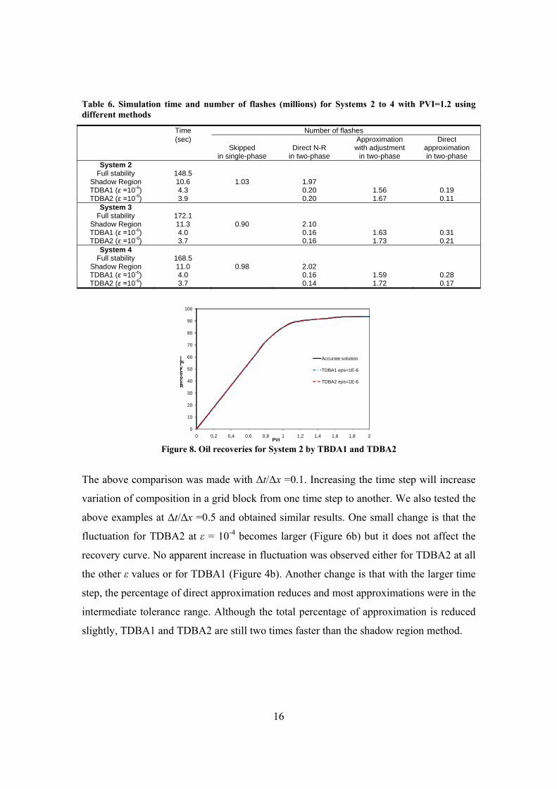
Since the results at tolerance ε = 10-6 seems to be accurate enough for both TDBA1 and

TDBA2, we use this tolerance for the tests of the other three systems. Table 6

summarizes the calculation results for three Zick oils (Systems 2, 3 and 4). The shadow

region method, TDBA1, TDBA2, and the full stability analysis method have been used.

The table gives detailed statistics on the number of flashes performed. The simulation

was performed for 1.2 PVI in 6000 time steps. For the full stability analysis, three million

flashes are performed with the traditional flash algorithm. For the shadow region method,

around one million flashes are in the single-phase and outside the shadow region, and

those flashes were skipped; around two million flashes are in the two-phase region, which

are calculated by the direct Newton-Raphson algorithm. For TDBA1 and TDBA2, there

are also around two million flashes in the two-phase region. Around 90% of them were

approximated: 5-10% of them by direct approximation using the old results, 80-85% of

them by approximation with adjustment. The high percentage of approximation makes

TDBA1 and TDBA2 much faster than the shadow region method. It should also be noted

that most approximations fall in the intermediate range. The approximation with

adjustment in this range is crucial to both speed and stability. The above observations on

simulation time and statistics of approximations are consistent with those in Table 5 for

System 1. Figure 8 shows the recovery curve for System 2. Although not shown here,

Systems 3 and 4 give essentially the same behavior. Again, TDBA1 and TDBA2 present

essentially the same recovery as the accurate solution.

16

Table 6. Simulation time and number of flashes (millions) for Systems 2 to 4 with PVI=1.2 using different methods

Time Number of flashes (sec)

Skipped in single-phase

Direct N-R

in two-phase

Approximation with adjustment

in two-phase

Direct approximation in two-phase

System 2 Full stability 148.5

Shadow Region 10.6 1.03 1.97 TDBA1 (ε =10-6) 4.3 0.20 1.56 0.19 TDBA2 (ε =10-6) 3.9 0.20 1.67 0.11





0

10

20

30

40

50

60

70

80

90

100

0 0,2 0,4 0,6 0,8 1 1,2 1,4 1,6 1,8 2

Recovery (%)

PVI

Accurate solution

TDBA1 eps=1E-6

TDBA2 eps=1E-6

Figure 8. Oil recoveries for System 2 by TBDA1 and TDBA2

The above comparison was made with Δt/Δx =0.1. Increasing the time step will increase

variation of composition in a grid block from one time step to another. We also tested the

above examples at Δt/Δx =0.5 and obtained similar results. One small change is that the

fluctuation for TDBA2 at ε = 10-4 becomes larger (Figure 6b) but it does not affect the

recovery curve. No apparent increase in fluctuation was observed either for TDBA2 at all

the other ε values or for TDBA1 (Figure 4b). Another change is that with the larger time

step, the percentage of direct approximation reduces and most approximations were in the

intermediate tolerance range. Although the total percentage of approximation is reduced

slightly, TDBA1 and TDBA2 are still two times faster than the shadow region method.

17

A potential use of the TDBA methods is to speed up simulation with advanced and

complicated EoS’s. A recent study by Yan et al. (2011) shows that by modifying the

algorithm, the simulation speed for non-cubic EoS’s, like the PC-SAFT EoS, can be

greatly improved. It is shown here that by integrating TDBA1 to the modified algorithm,

the simulation time required for a 1-D slimtube simulation with PC-SAFT can be

substantially reduced (Figure 9). The system tested in Figure 9 is a 6-component gas

injection system, the component list has been duplicated, triplicated, and quadruplicated

to study the influence of number of components on simulation time.

0

20

40

60

80

100

120

140

160

180

0 5 10 15 20 25 30

Simulation time (sec)

Number of components

SRK

CPA

PC‐SAFT

CPA new

PC‐SAFT new

SRK+TDBA

CPA+TDBA

PC‐SAFT+TDBA

0.0

1.0

2.0

3.0

4.0

5.0

6.0

7.0

8.0

0 5 10 15 20 25 30

Simulation time ratio

Number of components

CPA

PC‐SAFT

CPA new

PC‐SAFT new

CPA+TDBA w.r.t. SRK+TDBA

PC‐SAFT+TDBA w.r.t. SRK+TDBA

CPA+TDBA w.r.t. SRK

PC‐SAFT+TDBA w.r.t. SRK

(a) (b)

Figure 9. Simulation time results for a 6-component system (Yan et al., 2011) by using the reference method, the new method (Yan et al., 2011), and the new method + TDBA1: (a) simulation time; (b)

simulation time ratio of PC-SAFT and CPA to SRK.

3. Reduced variables methods

The reduced variables methods simplify the original phase equilibrium problem with a

smaller set of independent variables. The methods are designed for a cubic EoS where the

matrix of binary interaction parameters (BIPs) is of low rank. For the SRK EoS

( )

nRT AP

V B V V B

(8)

with

C

i ii

B b n C C

ij i ji j

A a n n (1 )ij ii jj ija a a k (9)

the fugacity coefficients can be expressed as

ˆln i n a i b iC C A C b (10)

18

If all the BIPs are zero, 2C

i ii ij jj

A a a n and

*ˆln i n a i b iC C A C b (11)

To our knowledge, using reduced variables for phase equilibrium calculation can be

traced back to 30 years ago when Michelsen and Heideman (1981) applied it to critical

point calculation. The method was first suggested for flash calculations by Michelsen in

1986. Michelsen (1986) showed that only three equations are needed to solve the flash

problem when all the BIPs are zero. Later, Jensen and Fredenslund (1987) extended the

method to calculations with single nonzero BIP row/column. Hendriks et al. (1992)

proposed a generalized reduced variables method that can deal with general non-zero BIP

matrices. The generalized method has been extensively used for the last 20 years by

different researchers (Firoozabadi and Pan, 2002; Pan and Firoozabadi, 2003; Nichita and

Minescu, 2004; Li and Johns, 2006; Nichita and Graciaa, 2010). Recently, the advantages

of the reduced variables method were questioned by Haugen and Beckner (2011).

There are some arguments against using reduction methods: they are essentially restricted

to the cubic EoS; they cannot so easily be formulated as unconstrained minimization

problems— consequently, they are less safe; the composition derivatives required by

second order methods are more cumbersome to set up; the simple algebraic operations

required to evaluate iA are very inexpensive today, as compared with what can be

achieved with the computing equipments in the 1980s; finally, although it is often

claimed that the effort of the conventional approach grows approximately proportionally

with C2 or even C3, our experience does show that the dependence of simulation time on

C is almost linear. The above arguments suggest that the potential for speeding up flash

calculation with reduced variables methods may be modest, which leads to a low

incentive to compare a reduced variables method with an efficient implementation of the

conventional flash method, such as Michelsen’s code, especially if extensive coding is

needed to develop a reduced variables program with Gibbs energy minimization. A recent

development by Nichita and Graciaa (2010) enabled an adaption to Michelsen’s existing

code with moderate modifications. In the following subsections, it will be first presented

how to make such an adaptation based on Nichita and Graciaa’s formulation. Then, an

19

alternative algorithm which directly utilizes the sparsity of the BIP matrix will be

introduced. Finally, a comparison of the reduced variables method, the “sparse” BIP

matrix method, and the conventional flash method will be given. It should be noted that

the conventional flash method is for “blind” flash calculation with both stability analysis

and phase split.

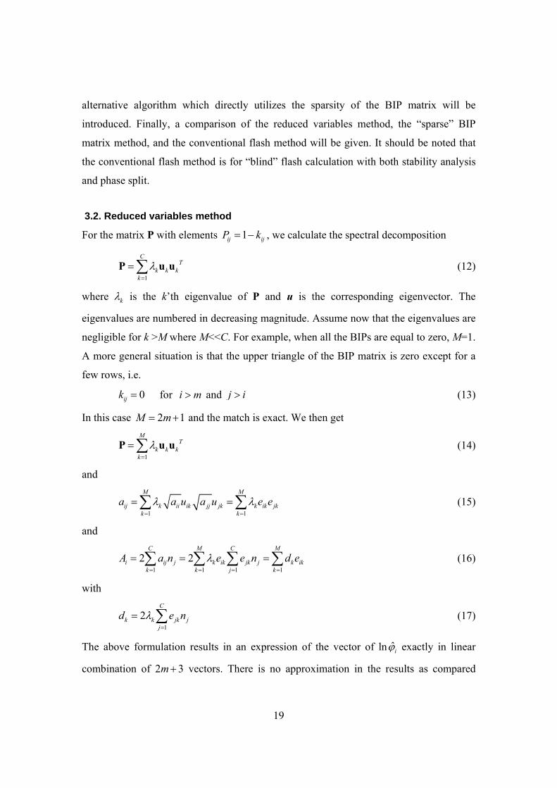
3.2. Reduced variables method

For the matrix P with elements 1ij ijP k , we calculate the spectral decomposition

1

CT

k k kk

P u u (12)

where k is the k’th eigenvalue of P and u is the corresponding eigenvector. The

eigenvalues are numbered in decreasing magnitude. Assume now that the eigenvalues are

negligible for k >M where M<<C. For example, when all the BIPs are equal to zero, M=1.

A more general situation is that the upper triangle of the BIP matrix is zero except for a

few rows, i.e.

0ijk for i m and j i (13)

In this case 2 1M m and the match is exact. We then get

1

MT

k k kk

P u u (14)

and

1 1

M M

ij k ii ik jj jk k ik jkk k

a a u a u e e

(15)

and

1 1 1 1

2 2C M C M

i ij j k ik jk j k ikk k j k

A a n e e n d e

(16)

with

1

2C

k k jk jj

d e n

(17)

The above formulation results in an expression of the vector of ˆln i exactly in linear

combination of 2 3m vectors. There is no approximation in the results as compared

20

with the full approach, while the computational effort is reduced from 2C to 2CM plus

overhead.

For the successive substitution step in both stability analysis and phase split, we follow

the conventional implementation except for calculation of Ai, which is calculated using

Eqs. (16) and (17). The acceleration step is used as usual. And there is no effect on

convergence behavior. The only difference is that the calculation of Ai is simplified.

For the second order minimization step, the expression of ln iK suggested by Nichita and

Graciaa (2010) is used. Nichita and Graciaa express ln iK as

2

1

lnM

i l ill

K c e

, , 1 1i Me , , 2i M ie b (18)

where c1, c2, …, and cM+2 are treated as independent variables. We express the gradients

required for minimization as

1

Ci

ij i j

vG G

c v c

, c g Wg (19)

where iv is vapor moles i and /ji i jW v c , which can be obtained from the Rachford-

Rice equation. The required Hessian matrix can be further derived as

c TH WHW (20)

Although Wji looks complex to calculate, simple algebraic expressions for the elements

can be derived. The final minimization procedure is

1. Calculate the K-factors from c

2. Solve the Rachford-Rice equation to get vi

3. Calculate “conventional” gradient and Hessian

4. Calculate transformation matrix W

5. Calculate c-based gradient and Hessian

6. Calculate corrected c using trust-region approach

A similar procedure can be developed for stability analysis.

21

3.3. An alternative simplification: sparse k

An alternative formulation to take advantage of the sparsity of the BIP matrix is proposed

here:

1

(1 ) ( )C

ii jj ij j ii ij

a a k n a S S

(21)

where

1

C

jj jj

S a n

(22)

and

1

1

C

jj ij jj

i m

jj ij jj

a k n i m

S

a k n i m

(23)

This formulation uses just approximately 2mC multiplications.

3.4. Results

Two tested mixtures used here are derived from the 9-component SPE3 mixture. The first

mixture is modified such that all kij = 0 for i > 3 and j > 3. Only the interaction parameters

with nitrogen, carbon dioxide, and methane are non-zero. For the second mixture,

nitrogen and carbon dioxide are removed, leaving just one row/column non-zero BIPs

and only five reduced variables. For both mixtures, the last species in the component list

is subdivided to increase C so that the influence of C on the simulation speed can be

tested. For all the three methods, including the reduced method, the “sparse” BIP matrix

method, and the conventional method, one million flash calculations are performed in an

equidistant 1000 by 1000 grid in T and P. All the calculations are “blind” with about 60%

in the two-phase region. The simulation time results are given in Figures 10 and 11. First,

for both mixtures and all three methods, the simulation times increase almost linearly

with C with a slight upward curvature only for very large C. This is also consistent with

our tests with more complicated EoS’s (Yan et al., 2011). If there are three rows/columns

of non-zero BIPs, the reduced variables method becomes slightly faster than the

22

conventional method only if C is larger than 20 (Figure 10). For the even simpler

situation with just one row/column non-zero BIPs, the speeding-up of the reduced

variables method is still very modest, with less than 20% reduction in time for C = 24

(Figure 11). A better reduction in simulation time can actually be obtained by simplifying

the Ai calculation using the sparsity of the BIP matrix.

Figure 10. Simulation times for the first mixture (three rows/columns non-zero BIPs)

Figure 11. Simulation times for the second mixture (just one row/column non-zero BIPs)

23

6. Conclusions

This paper summarizes two recent studies on fast flash methods. We have found

1. TTL, a variation of CSAT, approximates the flash results when the new feed is close

enough to an existing tie-line in the tie-line table. Although the time for rigorous flash is

saved, building and updating the tie-line table during the simulation leads to a non-

negligible overhead. The simulation time increases dramatically with the number of tie-

lines used. Big tolerances can lead to inaccurate results whereas small tolerances can lead

to very few uses of the tie-lines. TTL-PRE with a few pre-calculated tie-lines can

improve the speed as compared with performing rigorous flash calculations. However, at

small tolerances like 10-6 and 10-7, its speeding-up is very limited.

2. TDBA compares only the tie-line in the same grid block from a previous calculation so

that the task in managing the tie-line table is minimized. It speeds up the flash in the two-

phase region a lot, even at a tolerance of 10-7. At a tolerance of 10-5, the saturation profile

is already quite close to the rigorous solution. The recoveries are essentially the same

even for a tolerance of 10-4 for the systems studied here. TDBA also shows its potential to

speed up simulation with complicated EoS’s.

3. Compared with the conventional flash method, the reduced variable method is faster

only for large C and the speed-up is very modest. A better reduction in simulation time

can be obtained by a much simpler implementation, which directly takes advantage of the

sparsity of the BIP matrix.

Acknowledgements

The study on the table look-up methods was carried out under the CompSim project

sponsored by ENI S.p.A. The study on the reduced variables method was carried out

under the project “ADORE—Advanced Oil Recovery Methods” funded by the Danish

Council for Technology and Production Sciences, Maersk Oil, and DONG Energy.

24

References

Belkadi, A., Yan, W., Michelsen, M., Stenby, E.H., 2011. Comparison of Two Methods for Speeding Up

Flash Calculations in Compositional Simulations. Paper SPE 142132 presented at the SPE Reservoir

Simulation Symposium held in The Woodlands, Texas, USA, 21-23 February 2011.

Firoozabadi, A. and Pan, H. 2002. Fast and Robust Algorithm for Compositional Modeling: Part I –

Stability Analysis Testing. SPE J. 7 (1): 78-89.

Hendriks, E. M. 1988. Reduction Theorem for Phase Equilibria Problems. Industrial & Engineering.

Chemistry Research 27 (9): 1728-1732.

Li, Y. and Johns. R.T. 2006. Rapid Flash Calculations for Compositional Simulation. SPE Reservoir

Evaluation & Engineering 10: 521-529.

Jensen, B.H. and Fredenslund, A. 1987. A Simplified Flash Procedure for Multicomponent Mixtures

Containing Hydrocarbons and One Non-Hydrocarbon Using Two-Parameter Cubic Equations of State. Ind.

Eng. Chem. Res. 26 (10): 2129-2134.

Jessen, K. 2000. Effective Algorithms for the Study of Miscible Gas Injections Processes, PhD Dissertation,

Technical University of Denmark, Copenhagen, Denmark.

Haugen, K.B. and Beckner, B.L., 2011. Are Reduced Methods for EoS Calculations Worth the Effort?

Paper SPE 141399 presented at the SPE Reservoir Simulation Symposium held in The Woodlands, Texas,

USA, 21-23 February 2011.

Michelsen, M. L. 1982a. The Isothermal Flash Problem. Part I. Stability. Fluid Phase Equilibria 9 (1): 1–

19.

Michelsen, M. L. 1982b. The Isothermal Flash Problem. Part II. Phase-Split Calculation. Fluid Phase

Equilibria 9 (1): 21-40.

Michelsen, M.L. 1986. Simplified Flash Calculations for Cubic Equation of State. Industrial & Engineering

Chemistry Process Design and Development 25 (1): 184-188.

Michelsen, M. L. 1998. Speeding up the Two-Phase PT-Flash, with Applications for Calculation of

Miscible Displacement. Fluid Phase Equilibria 143 (1): 1-12.

Michelsen, M.L. and Heideman, R.A. 1981. Calculation of Critical Points from Cubic Two-Constant

Equations of State. AIChE J. 27, 521-523.

Michelsen, M. L. and Mollerup, J. M. 2007. Thermodynamic models: Fundamentals and Computational

Aspects, Second Edition, Holte, Denmark: Tie-line Publications.

Michael, M. L., 2011. Reduced Variables — Revisited. Presentation in the 2011 CERE Annual Discussion

Meeting, Hillerød, Denmark, 8-10 June 2011.

Nichita, D.V. and Graciaa, A. 2010. A New Reduction Method for Phase Equilibrium Calculations.

Proceedings of the 12th International Conference on Properties and Phase Equilibria for Product and

Process Design, Suzhou, China, 16-21 May 2010.

Nichita, D.V. and Minescu, F., 2004. Efficient Phase Equilibrium Calculation in a Reduced Flash Context.

Can. J. Chem. Eng. 82, 521-529.

25

Peng, D. Y. and Robinson, D. B. 1976. A New Two-Constant Equation of State. Industrial and Chemical

Engineering Fundamentals 15 (1): 59 -64.

Rasmussen, C. P., Krejberg, K., Michelsen, M. L., Bjurstrom, K. E. 2006. Increasing the Computational

Speed of Flash Calculations with Applications for Compositional Transient Simulations. SPE Reservoir

Evaluation & Engineering 9 (1): 32 – 38.

Soave, G. 1972. Equilibrium Constants from a Modified Redlich-Kwong Equation of State. Industrial and

Chemical Engineering Science 27 (6): 1197-1203.

Orr, F. M. 2007. Gas Injection Processes, Holte, Denmark: Tie-Line Publications.

Pan, H. and Firoozabadi, A. 2003. Fast and Robust Algorithm for Compositional Modeling: Part II - Two-

Phase Flash Computations. SPE J. 8 (4): 380-391.

Voskov, D. and Tchelepi, H. A. 2007. Compositional Space Parameterization for Flow Simulation. Paper

SPE 106029 presented at the SPE Reservoir Simulation Symposium Huston, Texas, USA, 26-28February.

Voskov, D. and Tchelepi, H. A. 2008a. Compositional Space Parameterization for Miscible Displacement

Simulation. Transport in Porous Media 75 (1): 111-128.

Voskov, D.V. and Tchelepi, H.A., 2008b. Compositional Parameterization for Multi-phase Flow in Porous

Media. Paper SPE 113492 presented at the 208 SPE/DOE Improved Oil Recovery Symposium, Tulsa,

Oklahoma, USA, 19-23 April.

Voskov, D. and Tchelepi, H. A. 2009. Tie-simplex Based Mathematical Framework for thermodynamical

Equilibrium Computation of Mixtures with an Arbitrary Number of Phases. Fluid Phase Equilibria 283 (1-

2): 1-11.

Yan, W., Michelsen, M. L., Stenby, E. H., Berenblyum, R. A., Shapiro, A. A. 2004. Three-phase

Compositional Streamline Simulation and Its Application to WAG. Paper SPE 89440 presented at the 2004

SPE/DOE 14th Symposium on Improved Oil Recovery, Tulsa, Oklahoma, USA, 17-21 April.

Yan, W., Michelsen, M.L., Stenby, E.H., 2011. On Application of Non-cubic EoS to Compositional

Reservoir Simulation. Paper SPE 142995 presented at the SPE EUROPEC/EAGE Annual Conference and

Exhibition held in Vienna, Austria, 23-26 May 2011.

Zick, A. A. 1986. A Combined Condensing/Vaporizing Mechanism in the Displacement of Oil by Enriched

Gases. Paper SPE 15493 presented at the 61st Annual Technical Conference and Exhibition of the Society

of Petroleum Engineers, New Orleans, USA, 5-8 October.

on two flash methods for compositional reservoir...

Documents