On Using Simple Time-of-Travel Capture ZoneDelineation Methodsby Admir Ceric1 and Henk Haitjema2

AbstractAs part of its Wellhead Protection Program, the U.S. EPA mandates the delineation of ‘‘time-of-travel capture

zones’’ as the basis for the definition of wellhead protection zones surrounding drinking water production wells.Depending on circumstances the capture zones may be determined using methods that range from simply drawinga circle around the well to sophisticated ground water flow and transport modeling. The simpler methods areattractive when faced with the delineation of hundreds or thousands of capture zones for small public drinkingwater supply wells. On the other hand, a circular capture zone may not be adequate in the presence of an ambientground water flow regime. A dimensionless time-of-travel parameter T~ is used to determine when calculatedfixed-radius capture zones can be used for drinking water production wells. The parameter incorporates aquiferproperties, the magnitude of the ambient ground water flow field, and the travel time criterion for the time-of-travel capture zone. In the absence of interfering flow features, three different simple capture zones can be useddepending on the value of T~. A modified calculated fixed-radius capture zone proves protective when T~ < 0.1,while a more elongated capture zone must be used when T~ >1. For values of T~ between 0.1 and 1, a circular cap-ture zone can be used that is eccentric with respect to the well. Finally, calculating T~ allows for a quick assessmentof the validity of circular capture zones without redoing the delineation with a computer model.

IntroductionThe delineation of time-of-travel capture zones is

important in the context of both ground water protection(EPA’s Wellhead Protection Program) and aquifer reme-diation. Delineating these capture zones can be difficultdue to the complex nature of the geological formationsthat make up the aquifer. In practice many of these com-plexities are ignored to arrive at a simple conceptualmodel of the aquifer suitable for the capture zone delin-eation process. Additionally, the lack of reliable fielddata and the cost of computer modeling form further in-centives to use as simple a model as possible. Althougha simple model may be convenient, the resulting capturezone may not be adequate.

The U.S. EPA (1987) suggests a series of delineationmethods, starting with a circle of arbitrary radius centeredat the well and progressing in complexity to full-blowncomputer modeling of solute transport. The arbitraryfixed-radius method, for instance, does not require anyhydrogeologic data and is quick and cheap. The resultingwellhead protection area (time-of-travel capture zone) israther arbitrary; however, it may or may not properly pro-tect the water supply well. Yet, because a state often hasseveral thousands of low-capacity (public) drinking waterwells for which a wellhead protection area is required,the arbitrary fixed radius is often the method of choicefor these systems. In reality, however, a circle does notalways offer a good approximation of the capture zonefor low-capacity wells, as they tend to have a very elon-gated rather than a circular shape. This is due to the factthat the ambient ground water flow usually dominates inthe presence of low-capacity wells, resulting in linear(uniform) rather than radial flow. An example of the useof the arbitrary fixed-radius method is found in the Well-head Protection Rule of Indiana (Indiana AdministrativeCode 1997), which allows for the use of a 3000-foot

1Corresponding author: Hydro-Engineering Institute, StjepanaTomica 1, 71000 Sarajevo, Bosnia and Herzegovina; (387) 33-212-467; fax (387) 33-207-949; aceric71@hotmail.com

2SPEA 439, Indiana University, Bloomington, IN 47405;haitjema@indiana.edu

Received May 28, 2003; accepted September 24, 2004.Copyright ª 2005 National Ground Water Association.

408 Vol. 43, No. 3—GROUND WATER—May–June 2005 (pages 408–412)

setback radius for wells with an average daily withdrawalof less than 100,000 gal/d. Although the application ofthe arbitrary fixed radius requires a prior approval fromthe Indiana Department of Environmental Management,the well’s discharge rate is the sole parameter that is con-sidered in granting the approval. Hydrogeologic andhydrologic parameters of the aquifer are not considered.The resulting uncertainty in the outcome of the delinea-tion is compensated for by the relatively large size of thecapture zone: a 3000-foot radius. The actual capture zone,however, is often a thin, pencil-shaped domain inside thiscircle or protruding out of it.

A compromise in the accuracy of the wellhead pro-tection area delineation is achieved by the use of analyti-cal methods. Most analytical models replace the ambientground water flow regime by a uniform flow in the areaof the well or wellfield. This simplification may beappropriate for a single well but is less suitable for well-fields, where well interference invalidates the uniform-ness of the ambient flow field.

Several authors have discussed the differencesbetween simple delineation methods and more compre-hensive numerical approaches to delineating capturezones. Cleary and Cleary (1991) discuss the theory andpractice of delineation techniques and point out thatnumerical methods demonstrate that subtle changes infield conditions may have large impacts on capture zones.Bogue (1994) evaluates several wellhead protection mod-els as part of a case study. He finds that while numericalmodels are more accurate, analytical models may still beadequate. Landmeyer (1994) found that numerical modelsperform better in the presence of ambient flow than doesthe calculated fixed-radius method. Livingstone et al.(1995) find that their three-dimensional numerical modelis more accurate than a two-dimensional numerical oranalytical model. Ahern et al. (2003) applied fixed-radius,analytic, hydrogeologic mapping, and numerical modelingtechniques. They conclude that the differences betweenthese techniques increase with increasing hydrogeologiccomplexity. None of these studies, however, offer a reli-able method to determine in advance which methodshould or can be used. The success or failure of, forinstance, the calculated fixed-radius method is onlyobserved after both this method and a more sophisticatedmethod, e.g., computer modeling, have been applied. This,of course, defeats the purpose of using a simple method.

In this paper we offer a simple decision criterion toselect between progressively more sophisticated capturezone delineation techniques. This criterion, a dimension-less time-of-travel parameter T~, provides insight into thepumping conditions and hydrogeologic conditions thatwill lead to a (nearly) circular capture zone. It appears thatthe ambient flow rate in the aquifer is the dominant factorin T~. We also suggest a variation on the classical calcu-lated fixed-radius capture zone delineation method tomake it more protective and extend its applicability. Ouranalyses, however, are based on the assumption that inter-ference of nearby wells or aquifer boundaries may beignored. We ignored areal recharge due to precipitation,which tends to lead to capture zones that are slightly toolarge but protective in view of wellhead protection.

Time-of-Travel Capture Zones for a Wellin a Uniform Flow Field

As the basis for our analysis, we consider the time-of-travel capture zone for a well in a uniform ambientflow field. The contours of the time-of-travel capturezones are constructed based on a solution obtained byBear and Jacobs (1965), who developed an expression forthe shape of the isochrones (advancing fronts) created bythe artificial replenishment of an aquifer through an injec-tion well. Bear and Jacobs (1965) considered a fully pen-etrating injection well, screened in a confined aquifer ofinfinite areal extent. The aquifer considered was of a con-stant thickness H (L), a constant effective porosity n (2),and a constant isotropic hydraulic conductivity k (L/T).The ambient ground water flow in the aquifer Qo (L2/T)was uniform. This ambient flow rate is the total flow inthe aquifer, integrated over the saturated aquifer thick-ness, per unit width of the aquifer. It is calculated by mul-tiplying the aquifer transmissivity (kH) by the regionalhydraulic gradient i:

Qo = kHi ð1Þ

The origin of a Cartesian x, y–coordinate system waslocated at the center of the well, with the x-axis orientedin the direction of the ground water flow Qo.

Adapting Bear and Jacobs’ solution for an extractionwell with discharge Q (L3/T) instead of an injection wellyields:

e2x~2T~ = cosðy~Þ2x~

y~sinðy~Þ ð2Þ

Variables x~ and y~ in Equation 2 are the dimensionless co-ordinates of a time-of-travel capture zone, defined as fol-lows:

x~ =x

Lsand y~ =

y

Lsð3Þ

where Ls (L) is the distance from the well to the well’sstagnation point (Haitjema 1995):

Ls =Q

2pQoð4Þ

The term T~ in Equation 2 is a dimensionless time-of-travel parameter, defined as:

T~ =T

Toð5Þ

where T is the time-of-travel (T) and To (T) a referencetime defined as:

To =nHQ

2pQ2o

ð6Þ

The reference time To may be physically interpreted asthe travel time from the well to the stagnation point of thewell in case the flow due to the well itself is ignored.

For an infinitely long time-of-travel, the time-of-travel capture zone will become the zone of contribution

A. Ceric, H. Haitjema GROUND WATER 43, no. 3: 408–412 409

(or capture zone envelope), inside which all ground waterwill eventually reach the well. The zone of contributionis the envelope of all time-of-travel capture zones and isderived from Equation 2 for T~/ N, which yields:

x~ =y~

tanðy~Þ ð7Þ

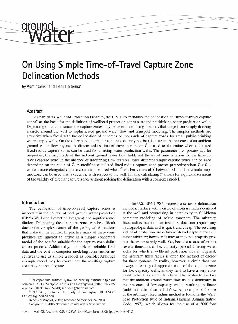
Figure 1 shows the contours of the time-of-travel capturezones that were constructed for some selected values ofthe parameter T~. These capture zones are represented bythe thin lines, while the thick line denotes the envelope ofthe capture zones as given by Equation 7.

Evaluation of Equation 2 to construct the time-of-travel capture zones shown in Figure 1 is cumbersomedue to the implicit nature of the equation. McElwee(1991) presented a similar diagram as shown in Figure 1using an iterative procedure to solve Equation 2, im-plemented in a Fortran program.

Approximate Time-of-Travel Capture ZonesThe results presented in Figure 1 are of use in evalu-

ating the applicability of simple capture zone delinea-tion methods without comparisons to more sophisticatedcomputer models. It is observed that the time-of-travel capture zones in Figure 1 are nearly circular inshape for sufficiently small values of the dimensionlesstime-of-travel parameter T~. The parameter T~, therefore,captures the essential parameters that determine theshape of the capture zone and follows from Equations 5and 6 as:

T~ =2pQ2

oT

nHQð8Þ

Of the parameters in Equation 8 the ambient flow rate Qo

(L2/T) plays the most significant role and is also the mostdifficult to determine, requiring an estimate of the aquifertransmissivity and the regional hydraulic gradient. Yet,once T~ has been calculated, the following can be saidabout the shape of the capture zone (Figure 1). For small

values of T~ (roughly for T~ smaller than 0.1), the time-of-travel capture zones resemble circles that appear to becentric with respect to the well. For values of T~ between0.1 and 1, the capture zones still resemble circles but areshifted into the direction from where the uniform flow iscoming. For values of T~ larger than 1, the time-of-travelcapture zones appear more like ellipses and cannot rea-sonably be approximated by circles.

These capture zones can be approximated withoutthe need to evaluate the transcendental Equation 2. To doso we define two characteristic dimensions of the capturezones shown in Figure 1. The distance from the well tothe furthest upgradient point of the time-of-travel capturezone is denoted by Lu, while the distance from the well tothe furthest downgradient point of the time-of-travel cap-ture zone is denoted by Ld. In dimensionless form wewrite:

Lu~ =LuLs

and Ld~ =LdLs

ð9Þ

The expression for the upgradient distance Lu~ may bederived from Equation 1 by substituting y~ = 0 andx~ = 2Lu~ , which after Equation 2 is rearranged yields(McElwee 1991):

Lu~ = T~1 lnð11 Lu~ Þ ð10Þ

Similarly, the downgradient distance Ld~ becomes:

Ld~ = 2T~2lnð12Ld~ Þ ð11Þ

Centric Circular Capture Zone (T~<0.1)For values of T~ of 0.1 and less, the ambient ground

water flow is small as compared to the pumping rate ofthe well, as indicated by Equation 8. In this case, it is pro-posed to approximate the actual time-of-travel capturezone with a circle centered at the well: a calculated fixed-radius capture zone. Traditionally, the radius is calculatedusing a water balance equation for a cylinder of water:

R2pHn = QT ð12Þ

Figure 1. Time-of-travel capture zones for several choices of T~.

410 A. Ceric, H. Haitjema GROUND WATER 43, no. 3: 408–412

where R is the radius of the cylinder around the well. Re-arranging Equation 12 yields the radius of the capture zonecalculated by the volumetric method (U.S. EPA 1987):

R =

ffiffiffiffiffiffiffiffiffiQT

pHn

rð13Þ

The radius in Equation 13 is only exact when the ambientground water flow is zero, otherwise it is not conservativewith respect to the corresponding time-of-travel capturezone for a well in a uniform flow. For the case of theapproximate circular capture zone proposed in this paper,some ambient flow may be present, since T~ may be aslarge as 0.1. To compensate for this, the radius R shouldbe selected such that it is 15% larger than the value inEquation 13:

R = 1:1543

ffiffiffiffiffiffiffiffiffiQT

pHn

rð14Þ

where 1.1543 is a correction factor that was calculatedsuch that the time-of-travel capture zone in Figure 1 fallsinside the circle with R obtained from Equation 14 andtouches for T~ = 0.1. This is illustrated in Figure 2, wherethe thin lines are the exact time-of-travel capture zonesfrom Figure 1 and the thick lines are circles with radiicalculated from Equation 14.

By use of Equations 4 and 8, Equation 14 may bewritten in dimensionless form:

R~ = 1:6324ffiffiffiT~

pð15Þ

where R̃=R=Ls:

Eccentric Circular Capture Zone (0.1< T~<1)For T~ larger than 0.1, but smaller than 1, a

time-of-travel capture zone can still be approximated by

a circle (Figure 1), but the circle has to be shiftedupgradient.

The diameter of the eccentric circle must be largeenough to enclose the actual time-of-travel capture zone(Figure 1), and thus the radius is R~ = (Lu~ 1 Ld~ )/2. Theeccentricity (shift) d~ then follows from d~~ ¼ ðLu~ 2Ld~ Þ=2.Both Lu~ and Ld~ are implicit in terms of T~ and will beapproximated for convenience of evaluation. We write R~

and d~ in dimensionless form as:

R~ = 1:1611 lnð0:391 T~Þ ð16Þ

and

d~ = 0:002781 0:652T~ ð17Þ

The form of Equations 16 and 17 follows from theobserved behavior of (Lu~ 1 Ld~ ) and (Lu~ 2 Ld~ ) in the rangeof 0.1 � T~� 1, while the constants have been chosen suchthat the eccentric circle always encloses the actual time-of-travel capture zone for 0.1 � T~�1 (Figure 3).

Boat-Shaped Capture Zone (T~[1)For T~ larger than 1, the time-of-travel capture zones

cannot reasonably be approximated by circles (Figure 1).In this case, it is proposed to replace the actual time-of-travel capture zone in Figure 1 by the envelope of all cap-ture zones, which is given by Equation 7. Expression 7 isexplicit in terms of y~ and thus much easier to evaluate.The upgradient boundary of the time-of-travel capturezone may be obtained by truncating Equation 7 atx~ = 2Lu~ as is illustrated in Figure 4. The approximatetime-of-travel capture zone (x~ = y~/tan(y~) and x~ = Lu~ ) isrepresented by the solid line in Figure 4 and always in-cludes the actual time-of-travel capture zone (dotted line).

Figure 2. Approximate capture zones (thick lines) and exactcapture zones (thin lines) for T~= 0.1, T~= 0.05, and T~= 0.01.

Figure 3. Approximate capture zones (thin lines) and exactcapture zones (thick lines) for T~= 1, T~= 0.5, and T~= 0.1.

A. Ceric, H. Haitjema GROUND WATER 43, no. 3: 408–412 411

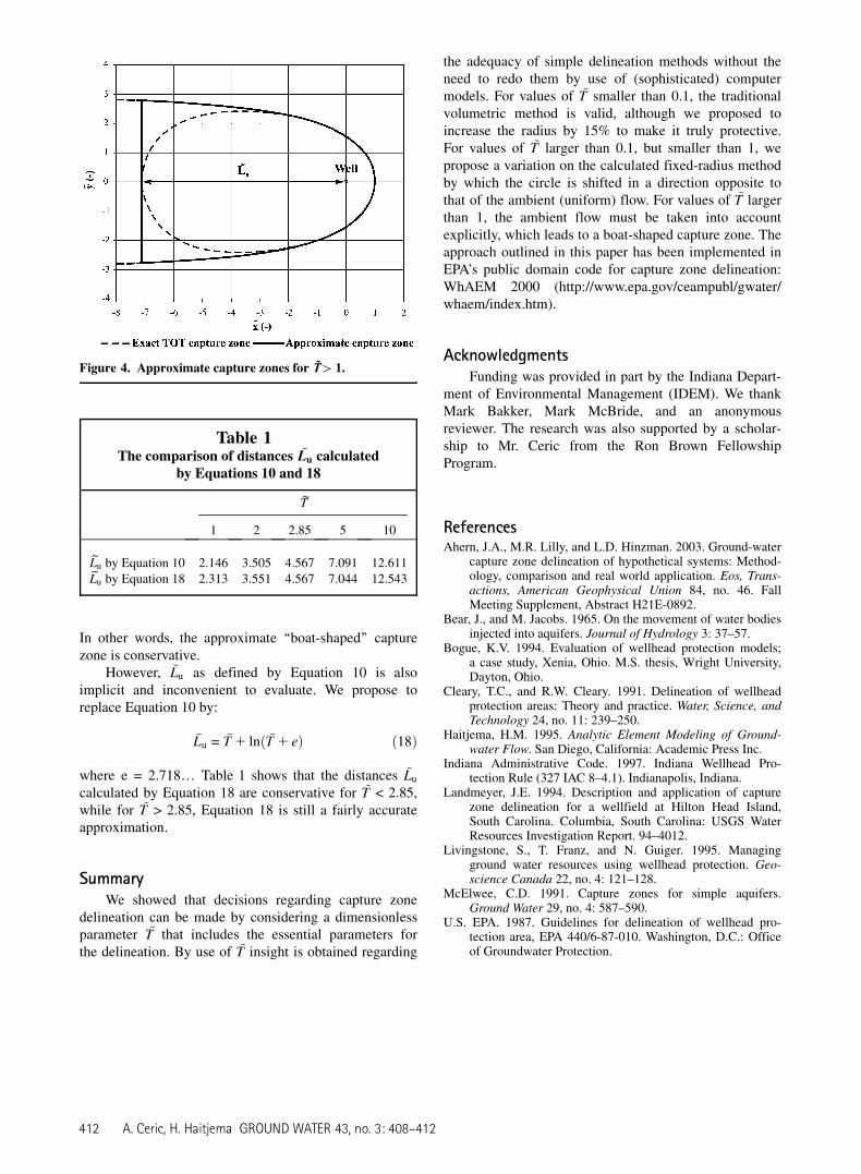
In other words, the approximate ‘‘boat-shaped’’ capturezone is conservative.

However, Lu~ as defined by Equation 10 is alsoimplicit and inconvenient to evaluate. We propose toreplace Equation 10 by:

Lu~ = T~1 lnðT~1 eÞ ð18Þ

where e = 2.718. Table 1 shows that the distances Lu~

calculated by Equation 18 are conservative for T~ < 2.85,while for T~ > 2.85, Equation 18 is still a fairly accurateapproximation.

SummaryWe showed that decisions regarding capture zone

delineation can be made by considering a dimensionlessparameter T~ that includes the essential parameters forthe delineation. By use of T~ insight is obtained regarding

the adequacy of simple delineation methods without theneed to redo them by use of (sophisticated) computermodels. For values of T~ smaller than 0.1, the traditionalvolumetric method is valid, although we proposed toincrease the radius by 15% to make it truly protective.For values of T~ larger than 0.1, but smaller than 1, wepropose a variation on the calculated fixed-radius methodby which the circle is shifted in a direction opposite tothat of the ambient (uniform) flow. For values of T~ largerthan 1, the ambient flow must be taken into accountexplicitly, which leads to a boat-shaped capture zone. Theapproach outlined in this paper has been implemented inEPA’s public domain code for capture zone delineation:WhAEM 2000 (http://www.epa.gov/ceampubl/gwater/whaem/index.htm).

AcknowledgmentsFunding was provided in part by the Indiana Depart-

ment of Environmental Management (IDEM). We thankMark Bakker, Mark McBride, and an anonymousreviewer. The research was also supported by a scholar-ship to Mr. Ceric from the Ron Brown FellowshipProgram.

ReferencesAhern, J.A., M.R. Lilly, and L.D. Hinzman. 2003. Ground-water

capture zone delineation of hypothetical systems: Method-ology, comparison and real world application. Eos, Trans-actions, American Geophysical Union 84, no. 46. FallMeeting Supplement, Abstract H21E-0892.

Bear, J., and M. Jacobs. 1965. On the movement of water bodiesinjected into aquifers. Journal of Hydrology 3: 37–57.

Bogue, K.V. 1994. Evaluation of wellhead protection models;a case study, Xenia, Ohio. M.S. thesis, Wright University,Dayton, Ohio.

Cleary, T.C., and R.W. Cleary. 1991. Delineation of wellheadprotection areas: Theory and practice. Water, Science, andTechnology 24, no. 11: 239–250.

Haitjema, H.M. 1995. Analytic Element Modeling of Ground-water Flow. San Diego, California: Academic Press Inc.

Indiana Administrative Code. 1997. Indiana Wellhead Pro-tection Rule (327 IAC 8–4.1). Indianapolis, Indiana.

Landmeyer, J.E. 1994. Description and application of capturezone delineation for a wellfield at Hilton Head Island,South Carolina. Columbia, South Carolina: USGS WaterResources Investigation Report. 94–4012.

Livingstone, S., T. Franz, and N. Guiger. 1995. Managingground water resources using wellhead protection. Geo-science Canada 22, no. 4: 121–128.

McElwee, C.D. 1991. Capture zones for simple aquifers.Ground Water 29, no. 4: 587–590.

U.S. EPA. 1987. Guidelines for delineation of wellhead pro-tection area, EPA 440/6-87-010. Washington, D.C.: Officeof Groundwater Protection.

Figure 4. Approximate capture zones for T~[ 1.

Table 1The comparison of distances Lu

~ calculatedby Equations 10 and 18

T~

1 2 2.85 5 10

Lu~

by Equation 10 2.146 3.505 4.567 7.091 12.611Lu~

by Equation 18 2.313 3.551 4.567 7.044 12.543

412 A. Ceric, H. Haitjema GROUND WATER 43, no. 3: 408–412