ONLINE APPENDIX

Unity in Diversity?

How Intergroup Contact Can Foster Nation Building

Samuel Bazzi∗Boston UniversityNBER and CEPR

Arya Gaduh†University of Arkansas

Alexander D. Rothenberg‡Syracuse University

Maisy Wong§University of Pennsylvania

July 2019

Abstract

This supplementary appendix comprises three sections. Section 1 presents additional empirical resultsand robustness checks. Section 2 derives our theoretical model of intergroup contact and presentssome simulation results of the model. Section 3 discusses the policy relevance and external validity ofour results. Finally, Section 4 is the data appendix.

∗Department of Economics. 270 Bay State Rd., Boston, MA 02215. Email: sbazzi@bu.edu.†Sam M. Walton College of Business. Department of Economics. Business Building 402, Fayetteville, AR 72701-1201. Email:

agaduh@walton.uark.edu.‡Syracuse University. 426 Eggers Hall. Syracuse, NY 13244-1020. Email: adrothen@maxwell.syr.edu.§Wharton Real Estate. 3620 Locust Walk, 1464 SHDH, Philadelphia, PA 19104-6302. Email: maisy@wharton.upenn.edu.

1

Contents

1 FURTHER EMPIRICAL RESULTS 2

1.1 Background Figures . . . . . . . . . . . . . . . . . . . . . . . . . . . . . . . . . . . . . . . . 2

1.2 Policy-Induced Variation in Diversity and Segregation . . . . . . . . . . . . . . . . . . . 3

1.3 Robust Inference . . . . . . . . . . . . . . . . . . . . . . . . . . . . . . . . . . . . . . . . . . 6

1.4 Own-Group Share and Overall Diversity . . . . . . . . . . . . . . . . . . . . . . . . . . . . 7

1.5 Probing Nonlinearities in F and P . . . . . . . . . . . . . . . . . . . . . . . . . . . . . . . 8

1.6 Native and Other Ethnic Language Use . . . . . . . . . . . . . . . . . . . . . . . . . . . . . 9

1.7 National Language Use by Education and Sector of Employment . . . . . . . . . . . . . 9

1.8 Addressing Sorting . . . . . . . . . . . . . . . . . . . . . . . . . . . . . . . . . . . . . . . . . 12

1.9 Addressing Location-by-Time Variation in Program Implementation of Diversity . . . 13

1.10 Parental Diversity . . . . . . . . . . . . . . . . . . . . . . . . . . . . . . . . . . . . . . . . . 14

1.11 Adjusting Children’s Names . . . . . . . . . . . . . . . . . . . . . . . . . . . . . . . . . . . 14

1.12 Further Results on Instrument Strength and Exogeneity . . . . . . . . . . . . . . . . . . . 15

2 MODEL APPENDIX 18

B.1 Intergroup Contact with a General Matching Function . . . . . . . . . . . . . . . . . . . . 18

B.2 Pairwise Proportional Imitation and the Replicator Dynamic . . . . . . . . . . . . . . . . 18

B.3 Village-level Growth Rate of Nationalists . . . . . . . . . . . . . . . . . . . . . . . . . . . 20

B.4 Evolutionary Equilibria . . . . . . . . . . . . . . . . . . . . . . . . . . . . . . . . . . . . . . 21B.4.1 5-Group Example . . . . . . . . . . . . . . . . . . . . . . . . . . . . . . . . . . . . . . 23B.4.2 Approximating Village-Level Tipping Points . . . . . . . . . . . . . . . . . . . . . . 24B.4.3 5-Group Simulations . . . . . . . . . . . . . . . . . . . . . . . . . . . . . . . . . . . . 27

3 THE TRANSMIGRATION PROGRAM: POLICY IMPLICATIONS AND EXTERNAL VALIDITY 28

4 DATA APPENDIX 30

D.1 Transmigration Census and Maps . . . . . . . . . . . . . . . . . . . . . . . . . . . . . . . . 31

D.2 Demographic and Socioeconomic Variables . . . . . . . . . . . . . . . . . . . . . . . . . . 31

D.3 Spatial, Topographical, and Agroclimatic Variables . . . . . . . . . . . . . . . . . . . . . 34

D.4 Linguistic Distance: World Language Mapping System (WLMS) and Ethnologue . . . . 36

REFERENCES 37

1

1 Further Empirical Results

1.1 Background Figures

Figure 1 plots mean (a) national and (b) native ethnic language use against the share of one’s own ethnicgroup in the village. The local-linear regression is at the village × own-group-share level based on thefull population of roughly 1.8 million individuals aged 5+ across 817 Transmigration villages.

Figure 1: Own-Group Share and Language Use at Home

(a) National Language (b) Native Ethnic Language

Notes: These local-linear regressions use an Epanechnikov kernel and rule-of-thumb bandwidth, and the dashed lines are95 percent confidence intervals.

Figure 2 plots the joint kernel density of ethnic fractionalization and polarization in 2010 for (a) Trans-migration villages and (b) non-Transmigration villages in the Outer Islands.

Figure 2: Transmigration Generated Joint Variation in Fractionalization and Polarization

(a) Transmigration Villages (b) Non-Transmigration Villages

Notes: Both densities employ an Epanechnikov kernel and rule-of-thumb bandwidth.

2

1.2 Policy-Induced Variation in Diversity and Segregation

Table 1 shows that Transmigration villages have significantly lower residential segregation across ethnicgroups compared to non-Transmigration villages with nearly identical levels of overall diversity. Wemeasure diversity (F and P ) and segregation (S, see Section VII.A) using the 2010 Census. We considertwo comparison groups. Columns 1 and 2 compare Transmigration villages to all non-Transmigrationvillages at least 10 km from Transmigration village boundaries in 2000. Columns 3 and 4 compare Trans-migration villages to planned settlements that never received the program as a result of budget cutbacks(see Bazzi et al., 2016). These “almost-treated” villages have similar natural advantages to the Transmi-gration villages we study, but the budget shock meant that they were gradually developed through aprocess of spontaneous settlement that was not managed by the federal government.

Table 1: Policy-Induced Residential Segregation in Transmigration VillagesControl Group

Non-Transmigration “Almost-Treated”Villages Villages

(1) (2) (3) (4)

Transmigration village -0.006 -0.004 -0.012 -0.010(0.002) (0.002) (0.004) (0.003)

Number of Villages 23,562 23,562 1,514 1,514Dependent Variable Mean 0.020 0.020 0.029 0.029R2 0.262 0.305 0.225 0.383

Function of F , P Decile Percentile Decile Percentile

Notes: The dependent variable is the Alesina and Zhuravskaya (2011) of residential segregation in 2010. The Transmi-gration village indicator equals for all Transmigration villages in our study. The control group varies across columns 1–2and 3–4 as detailed above. Columns 1 and 3 include indicators for the decile of village-level ethnic fractionalization andpolarization. Columns 2 and 4 include indicators for the percentile of village-level ethnic fractionalization and polariza-tion. These regressions also control for the same natural advantages (x) and island fixed effects as our baseline regression.Standard errors are clustered by district.

Looking across columns, Transmigration villages have around one-quarter to one-third less ethnicsegregation than comparable villages with similar F and P . These conclusions hold whether we definecomparable diversity using deciles or percentiles of F and P . As discussed in Section V.B, the lottery-based assignment of housing plots (and delayed property rights) help explain the persistently lowersegregation in Transmigration villages.

3

Table 2: Long-Run Diversity, Locational Fundamentals, and Pre-Program DevelopmentDistrict-Level Population Characteristics, 1978

Dependent Variable: distance to log ruggedness total Indonesian radio television agriculture trade/service wagedistrict cap. major road coast river altitude index population use at home ownership ownership empl. share empl. share empl. share

(1) (2) (3) (4) (5) (6) (7) (8) (9) (10) (11) (12) (13)

Panel A: Transmigration Villages

ethnic fractionalization 0.146 0.019 -0.498 0.048 -1.061 0.018 -0.267 0.034 0.009 -0.005 0.028 -0.002 -0.019(0.528) (0.041) (0.402) (0.299) (1.286) (0.047) (0.351) (0.038) (0.040) (0.022) (0.044) (0.033) (0.027)

ethnic polarization -0.241 -0.008 0.654 0.182 0.899 -0.030 -0.178 -0.020 -0.006 0.008 -0.034 0.002 0.047(0.432) (0.031) (0.307) (0.257) (1.093) (0.045) (0.254) (0.024) (0.030) (0.016) (0.032) (0.022) (0.021)

Number of Villages 817 817 817 817 817 817 817 817 817 817 817 817 817Dependent Variable Mean 4.122 0.079 10.557 8.084 3.284 0.311 12.505 0.072 0.463 0.069 0.780 0.150 0.121R2 0.014 0.011 0.216 0.063 0.007 0.046 0.240 0.473 0.556 0.087 0.032 0.024 0.034

Panel B: Non-Transmigration Villages in the Outer Islands

ethnic fractionalization -2.166 -0.048 -0.898 -0.141 -2.140 -0.007 -0.436 0.165 0.032 0.109 -0.166 0.144 0.114(0.288) (0.016) (0.263) (0.161) (0.412) (0.026) (0.233) (0.051) (0.021) (0.043) (0.086) (0.073) (0.047)

ethnic polarization 1.465 0.027 0.503 0.164 0.701 -0.005 0.294 -0.043 0.016 -0.053 0.109 -0.097 -0.054(0.207) (0.012) (0.276) (0.124) (0.357) (0.021) (0.163) (0.034) (0.016) (0.029) (0.059) (0.050) (0.032)

Number of Villages 26,119 29,158 29,158 29,158 26,119 29,158 22,400 22,400 22,400 22,400 22,400 22,400 22,400Dependent Variable Mean 3.517 0.069 9.727 7.977 3.804 0.277 12.667 0.084 0.427 0.072 0.759 0.166 0.133R2 0.067 0.136 0.271 0.041 0.090 0.071 0.235 0.329 0.689 0.146 0.077 0.080 0.069

Notes: The dependent variable is as defined at the top of each column. Sample sizes vary across columns due to matching original data sources with contemporaryvillages. Standard errors are clustered by district.

4

Panel A of Table 2 shows that diversity (F and P ) in Transmigration villages in 2010 appears to be un-correlated with natural advantages and predetermined correlates of nation building. In contrast, PanelB documents systematic correlations with diversity in non-Transmigration villages. These correlates in-clude physical natural advantages: (1) distance to historic district capitals, (2) distance to the nearestmajor road, (3) distance to the coast, (4) distance to the nearest river, (5) log altitude, and (6) terrainruggedness.1 Other correlates measure the characteristics of populations living in nearby areas withinthe same district before the Transmigration program, using the 1980 Population Census and restrictingto those living in the district in 1978.2 These include: (7) total district population, (8) Indonesian use athome, (9) radio ownership, (10) television ownership, (11) agriculture, (12) trade and services, and (13)wage-based employment shares. Each column of Table 2 regresses correlate y listed at the top of tableon the ethnic fractionalization and polarization observed in each village in 2010. Together, the stark dif-ferences across Panels A and B point to the plausibly exogenous variation in long-run diversity offeredby Transmigration program.

1See Appendix D.3 for a discussion fo these variables.2These variables are based on data from the 1980 Census sample available on IPUMS International, (ii) measured at the districtlevel based on 1980 district boundaries, (iii) computed using the sampling weights needed to recover district-level populationsummary statistics, and (iv) restricted to the population in each district that did not arrive as immigrants in 1979 or earlier in1980 (i.e., the still living population residing in the district in 1978).

5

1.3 Robust Inference

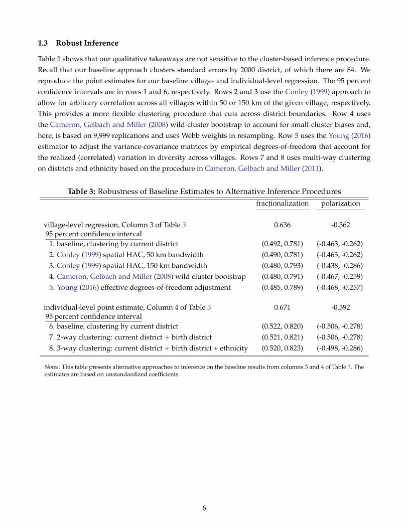
Table 3 shows that our qualitative takeaways are not sensitive to the cluster-based inference procedure.Recall that our baseline approach clusters standard errors by 2000 district, of which there are 84. Wereproduce the point estimates for our baseline village- and individual-level regression. The 95 percentconfidence intervals are in rows 1 and 6, respectively. Rows 2 and 3 use the Conley (1999) approach toallow for arbitrary correlation across all villages within 50 or 150 km of the given village, respectively.This provides a more flexible clustering procedure that cuts across district boundaries. Row 4 usesthe Cameron, Gelbach and Miller (2008) wild-cluster bootstrap to account for small-cluster biases and,here, is based on 9,999 replications and uses Webb weights in resampling. Row 5 uses the Young (2016)estimator to adjust the variance-covariance matrices by empirical degrees-of-freedom that account forthe realized (correlated) variation in diversity across villages. Rows 7 and 8 uses multi-way clusteringon districts and ethnicity based on the procedure in Cameron, Gelbach and Miller (2011).

Table 3: Robustness of Baseline Estimates to Alternative Inference Proceduresfractionalization polarization

village-level regression, Column 3 of Table 3 0.636 -0.36295 percent confidence interval

1. baseline, clustering by current district (0.492, 0.781) (-0.463, -0.262)2. Conley (1999) spatial HAC, 50 km bandwidth (0.490, 0.781) (-0.463, -0.262)3. Conley (1999) spatial HAC, 150 km bandwidth (0.480, 0.793) (-0.438, -0.286)4. Cameron, Gelbach and Miller (2008) wild cluster bootstrap (0.480, 0.791) (-0.467, -0.259)5. Young (2016) effective degrees-of-freedom adjustment (0.485, 0.789) (-0.468, -0.257)

individual-level point estimate, Column 4 of Table 3 0.671 -0.39295 percent confidence interval

6. baseline, clustering by current district (0.522, 0.820) (-0.506, -0.278)7. 2-way clustering: current district + birth district (0.521, 0.821) (-0.506, -0.278)8. 3-way clustering: current district + birth district + ethnicity (0.520, 0.823) (-0.498, -0.286)

Notes: This table presents alternative approaches to inference on the baseline results from columns 3 and 4 of Table 3. Theestimates are based on unstandardized coefficients.

6

1.4 Own-Group Share and Overall Diversity

Table 4 shows that our results for F and P are not an artifact of variation in the size of one’s own ethnicgroup in the village. Rather, in multi-ethnic communities like Transmigration villages, F and P conveyadditional information about the size of one’s own group relative to multiple other groups. Columns 1, 4and 7 reproduce the baseline individual-level estimates from columns 4,5, and 6 of Table 3, respectively.Columns 2, 5, and 7 control for the share of an individual’s ethnic group in the village. Columns 3, 6, 9control for the decile of that share with the top decile being the highest shares. Looking across columns,we find that conditioning on own-group-share reduces the effect of F but leaves the effects of P mostlyunchanged. Both F and P retain their economic significance.

Table 4: Distinguishing the Effects of Own-Group Share(1) (2) (3) (4) (5) (6) (7) (8) (9)

ethnic fractionalization 0.146 0.062 0.104 0.108 0.049 0.085 0.082 0.026 0.056(0.016) (0.016) (0.016) (0.012) (0.013) (0.014) (0.011) (0.011) (0.010)

ethnic polarization -0.086 -0.086 -0.093 -0.066 -0.063 -0.071 -0.040 -0.038 -0.042(0.013) (0.013) (0.014) (0.009) (0.009) (0.012) (0.008) (0.009) (0.010)

own-group share -0.387 -0.371 -0.357(0.021) (0.032) (0.026)

bottom decile, own-group share 0.429 0.384 0.367(0.036) (0.037) (0.035)

2nd decile, own-group share 0.222 0.220 0.214(0.038) (0.035) (0.034)

3rd decile, own-group share 0.101 0.109 0.127(0.040) (0.036) (0.036)

4th decile, own-group share 0.117 0.109 0.106(0.043) (0.037) (0.034)

5th decile, own-group share 0.106 0.084 0.081(0.043) (0.037) (0.037)

6th decile, own-group share 0.105 0.087 0.072(0.034) (0.029) (0.029)

7th decile, own-group share 0.110 0.089 0.077(0.033) (0.028) (0.026)

8th decile, own-group share 0.053 0.039 0.034(0.024) (0.021) (0.021)

9th decile, own-group share 0.023 0.016 0.023(0.014) (0.012) (0.016)

Number of Individuals 1,800,499 1,800,499 1,800,499 1,800,499 1,800,499 1,800,499 1,800,499 1,800,499 1,800,499Dependent Variable Mean 0.154 0.154 0.154 0.154 0.154 0.154 0.154 0.154 0.154R2 0.114 0.178 0.199 0.223 0.246 0.256 0.281 0.302 0.308Island FE, x Controls X X X X X X X X XEthnicity, Age, Gender FE X X X X X XBirth District, Current District FE X X X

Notes: The dependent variable is national language use at home. Standard errors are clustered by district.

7

1.5 Probing Nonlinearities in F and P

Table 5 reports the point estimates on the indicators for interactions of fractionalization F quintile i andpolarization P quintile j (FiPj) according to equation (8). These point estimates are used to generateFigure 4(b) by adding the mean for F1P1 at the bottom of the table to each coefficient estimate.

Table 5: Regression Results Underlying Figure 4(1)

F1P2 0.036(0.025)

F2P1 -0.035(0.032)

F2P2 0.050(0.014)

F2P3 -0.017(0.016)

F3P2 0.366(0.173)

F3P3 0.106(0.022)

F3P4 0.044(0.019)

F3P5 -0.034(0.020)

F4P3 0.210(0.040)

F4P4 0.140(0.034)

F4P5 0.061(0.022)

F5P2 0.415(0.074)

F5P3 0.263(0.043)

F5P4 0.166(0.030)

F5P5 0.080(0.023)

Number of Villages 817Dep. Var. Mean: F1P1 0.036R2 0.457

Notes: Standard errors are clustered by district.

8

1.6 Native and Other Ethnic Language Use

Table 6 reproduces the baseline individual-level estimates from columns 4–6 of Table 3 for national lan-guage use at home. After these first three columns 1-3, columns 4–6 (7–9) change the dependent variableto indicate whether the individual speaks his/her native ethnic (another group’s ethnic) language athome. The three columns are mutually exhaustive of potential language choices.

1.7 National Language Use by Education and Sector of Employment

Tables 7 and 8 estimate the full fixed effects, individual-level specification (column 6 of Table 3) sepa-rately by education and occupation, respectively. The estimates for F and P reflect standardized effectsof a one s.d. increase.

In Table 7, the baseline estimate from column 6 of Table 3 is reproduced in column 1. Each subse-quent column splits the sample to include only those with the education level listed at the top of thecolumn. An individual’s education is coded as either the highest level attained or the level in which thatindividual is currently enrolled. We find similar effects of F and P if we restrict our specifications onlyto individuals who have finished schooling, or to individuals who are currently enrolled. We also findsimilar effects on individuals with co-resident parents who have completed different educational levels.

In Table 8, we restrict to working-age individuals. Column 1 includes the full working-age popula-tion, and column 2 restricts to those not currently employed. Columns 3–7 consider mutually exhaustiveemployment sector categories: (3) agriculture and mining, (4) manufacturing, (5) electricity, constructionand transport, which we group together as “manual”, (6) trade and services, (7) health, education andpublic sector, which we group together as “white collar”, and (8) all other occupations.

9

Table 6: Ethnic Diversity and Language Use At HomeDep. Var.: Individual Speaks [. . . ] as Main Language at Home

Indonesian Native Ethnic Other Ethnic(1) (2) (3) (4) (5) (6) (7) (8) (9)

ethnic fractionalization 0.146 0.108 0.082 -0.182 -0.117 -0.080 0.036 0.008 -0.002(0.016) (0.012) (0.011) (0.015) (0.010) (0.009) (0.012) (0.008) (0.008)

ethnic polarization -0.086 -0.066 -0.040 0.088 0.066 0.042 -0.002 -0.000 -0.002(0.013) (0.009) (0.008) (0.011) (0.008) (0.008) (0.010) (0.008) (0.006)

Number of Individuals 1,800,499 1,800,499 1,800,499 1,800,499 1,800,499 1,800,499 1,800,499 1,800,499 1,800,499Dependent Variable Mean 0.154 0.154 0.154 0.764 0.764 0.764 0.082 0.082 0.082R2 0.114 0.221 0.280 0.129 0.323 0.370 0.071 0.249 0.294

Island FE, x Predetermined Controls X X X X X X X X XEthnicity, Age, Gender FE X X X X X XBirth District, Current District FE X X X

Notes: Standard errors are clustered by district.

10

Table 7: Ethnic Diversity and National Language Use At Home by Educationbaseline no school primary secondary

some completed junior senior post-(1) (2) (3) (4) (5) (6) (7)

ethnic fractionalization 0.082 0.057 0.082 0.072 0.088 0.095 0.057(0.011) (0.009) (0.012) (0.010) (0.013) (0.013) (0.016)

ethnic polarization -0.040 -0.029 -0.036 -0.042 -0.042 -0.028 -0.006(0.008) (0.007) (0.010) (0.007) (0.010) (0.013) (0.014)

Number of Individuals 1,800,499 141,545 408,269 650,912 336,498 198,334 64,070Dependent Variable Mean 0.154 0.116 0.165 0.102 0.156 0.260 0.347R2 0.281 0.324 0.308 0.250 0.276 0.294 0.304

Notes: Following the specification in column 6 of Table 3, these regressions include the baseline village-level x controls as well as fixed effects for individual age, gender,ethnicity, birth district, origin district, and relation to the household head. Standard errors are clustered by district.

Table 8: Ethnic Diversity and National Language Use At Home by Sector of Employmentbaseline not working agri/mine manuf. manual trade/svc white collar other

(1) (2) (3) (4) (5) (6) (7) (8)

ethnic fractionalization 0.080 0.089 0.058 0.075 0.107 0.081 0.071 0.092(0.011) (0.013) (0.008) (0.016) (0.015) (0.012) (0.016) (0.017)

ethnic polarization -0.041 -0.042 -0.034 -0.026 -0.057 -0.035 -0.018 -0.028(0.008) (0.010) (0.007) (0.012) (0.014) (0.011) (0.015) (0.015)

Number of Individuals 1,590,709 685,523 640,488 21,372 27,246 97,930 87,272 10,374Dependent Variable Mean 0.143 0.165 0.085 0.163 0.152 0.191 0.305 0.205R2 0.276 0.286 0.241 0.336 0.327 0.280 0.313 0.325

Notes: Following the specification in column 6 of Table 3, these regressions include the baseline village-level x controls as well as fixed effects for individual age, gender,ethnicity, birth district, origin district, and relation to the household head. Standard errors are clustered by district.

11

1.8 Addressing Sorting

Table 9 includes additional fixed effects to control for confounding effects of endogenous sorting alongorigin–destination or ethnicity–destination pairs. Column 1 reproduces column 6 of Table 3.

Table 9: Additional Fixed Effects(1) (2) (3)

ethnic fractionalization 0.082 0.083 0.081(0.011) (0.011) (0.011)

ethnic polarization -0.040 -0.039 -0.040(0.008) (0.009) (0.009)

Number of Individuals 1,800,499 1,800,499 1,800,499Dependent Variable Mean 0.154 0.153 0.153R2 0.282 0.318 0.344Ethnicity Fixed Effects X XBirth District + Current District Fixed Effects XBirth District × Current District Fixed Effects XEthnicity × Current District Fixed Effects X

Notes: Standard errors are clustered by district.

Table 10 augments the full fixed effects, individual-level specification in column 6 of Table 3 (reproducedin column 1 below) to account for the share of the population that may have endogenously sorted. Weidentify as sorters the share of the village population that we classified in column 7 of Table 5 as long-distance sorters. This includes all individuals born in other Outer-Island provinces, which would nothave been eligible to join the given village as part of the APPDT allotment. These long-distance migrantsthat plausibly arrived after the initial year of settlement include individuals of Outer- and Inner-Islandethnicities. The latter include non-indigenous ethnic communities in the Outer Islands, some of whommay have resided there for several generations. We control for ventiles of the village-level populationshares of each of these groups in columns 2–4. This slightly reduces the effects of F and P but mostlyleaves the results unchanged.

Table 10: Further Checks on SortingDep. Var.: National Language Use at Home

(1) (2) (3) (4)

ethnic fractionalization 0.082 0.063 0.075 0.061(0.011) (0.012) (0.011) (0.012)

ethnic polarization -0.040 -0.036 -0.036 -0.033(0.008) (0.008) (0.009) (0.009)

Number of Individuals 1,800,499 1,800,499 1,800,499 1,800,499Dependent Variable Mean 0.154 0.154 0.154 0.154R2 0.281 0.285 0.287 0.290Ventiles of Share of Outer Ethnicity Sorters X XVentiles of Share of Inner Ethnicity Sorters X X

Notes: Standard errors are clustered by district.

12

1.9 Addressing Location-by-Time Variation in Program Implementation of Diversity

Table 11 includes an array fixed effects that account for unobservable variation in program implementa-tion and local conditions. In column 1, we reproduce the baseline village-level specification in column3 of Table 3. In subsequent columns, we add fixed effects for (2) the year of settlement, (3) the yearof settlement by island, (4) the year of settlement by province, (5) the year of settlement by district, (6)the ethnolinguistic homeland, and (7) the ethnolinguistic homeland by year of settlement. We definethe ethnolinguistic homeland of each village based on the ethnolinguistic group whose homeland poly-gon covers the most area of the village. These homelands correspond to the group that is native to thegiven region, according to the Ethnologue and World Language Mapping Study (WLMS). We are miss-ing this homeland polygon information for a few villages due to omissions in the WLMS shapefiles (seeAppendix 4).

Looking across columns, the effects of F and P remain stable. This suggests that there is limitedregion-specific confounding of the sort that one might worry about, e.g., if planners adjusted diversityto better match local receptiveness to integration.

Table 11: Robustness to Confounding Variation in Program Implementation and Local Con-ditions

(1) (2) (3) (4) (5) (6) (7)

ethnic fractionalization 0.135 0.129 0.130 0.123 0.114 0.121 0.127(0.015) (0.015) (0.015) (0.015) (0.023) (0.015) (0.022)

ethnic polarization -0.083 -0.081 -0.082 -0.073 -0.058 -0.069 -0.071(0.012) (0.012) (0.012) (0.012) (0.019) (0.012) (0.019)

Number of Villages 817 817 817 817 817 813 813Dependent Variable Mean 0.144 0.144 0.144 0.144 0.144 0.145 0.145R2 0.437 0.447 0.477 0.648 0.795 0.556 0.704Year Placed FE XIsland × Year Placed FE XProvince × Year Placed FE XDistrict × Year Placed FE XEthnolinguistic Homeland FE XEthnolinguistic Homeland × Year Placed FE X

Notes: Standard errors are clustered by district.

13

1.10 Parental Diversity

Table 12 shows that the effects of diversity on national language use at home are not driven solely byintermarried households. We retain the full fixed effects specification from column 6 of Table 3 butrestrict the sample to children of the household head and to households with both a head and spouse.Column 2 restricts to children with parents in an interethnic marriage while column 5 looks at childrenwith parents of the same ethnicity.

Table 12: Ethnic Diversity and National Language Use At Home by Parental Diversitybaseline parents interethnic

yes no(1) (2) (3)

ethnic fractionalization 0.093 0.062 0.084(0.014) (0.018) (0.014)

ethnic polarization -0.042 -0.010 -0.043(0.011) (0.014) (0.011)

Number of Individuals 585,318 76,830 508,423Dependent Variable Mean 0.182 0.486 0.136R2 0.300 0.332 0.275

Notes: Standard errors are clustered by district.

1.11 Adjusting Children’s Names

In Table 13, we consider alternative indices that are based on an aggregation of similar-sounding chil-dren’s names using a double-metaphone procedure detailed in Appendix D.2. The effects of F and P aresomewhat smaller than with the unadjusted names we use as a baseline in Table 9. This is not surprisinggiven that adjustment procedure reduces the amount of variation across names.

Table 13: Double Metaphone Adjustment of Children’s Names in Table 9Dep. Var.: precision of name in identifying . . .

Indonesian intermarried urban own-ethnicitylanguage home household

(1) (2) (3) (4)

ethnic fractionalization 0.109 0.106 0.157 -0.133(0.026) (0.026) (0.032) (0.037)

ethnic polarization -0.064 -0.070 -0.111 0.056(0.022) (0.022) (0.026) (0.027)

Number of Individuals 790,705 789,234 790,739 776,205R2 0.064 0.080 0.063 0.081

Notes: Standard errors are clustered by district.

14

1.12 Further Results on Instrument Strength and Exogeneity

This section provides additional details on the two sets of instruments isolating policy-induced variationin F and P in 2010 as detailed at the end of Section V.D: (i) the number of initial transmigrants from theInner Islands of Java/Bali, and (ii) the ethnic composition of those transmigrants from Java/Bali.

Appendix Figure 3, estimated using the Robinson (1988) semiparametric approach conditional on x,shows that the initial assignment of transmigrants strongly predicts Inner-Island ethnic shares in 2010.This strong relationship is consistent with barriers to mobility making it harder for settlers to leave theirinitially-assigned communities. Together, these frictions limited tipping, as evidenced by the roughly(log-)linear relationship.

Figure 3: Initial Transmigrant Assignment and Long-Run Inner-Island Ethnic Share

Notes: This figure reports a semiparametric Robinson (1988) regression and 95 percent confidence interval of the Inner-Island ethnic share in 2010 on the log of the transmigrant population from Java/Bali placed in that village in the initialyear of settlement. The local linear regression is conditional on island fixed effects and the vector x of predetermined siteselection variables described in the paper, and it is estimated based on an Epanechnikov kernel, Fan and Gijbels (1996)rule-of-thumb bandwidth, and trimming of the top 5th and bottom 1st percentile for presentational purposes.

Subsequent results in Appendix Figures 4 and 5 provide evidence supporting the exogeneity ofthe initial number of transmigrants. Figure 4 shows that planners did not systematically assign moretransmigrants to locations with greater (a) the linguistic similarity between the indigenous Outer-Islandgroup and Inner-Island settlers, (b) Indonesian use at home in 1980 in areas near the eventual Transmi-gration village, or (c) post-program immigration between 1995 and 2000. As discussed in Section V.D,this suggests that more transmigrants were not sent to locations with an initial predisposition towardsnational integration or immigrants. Figure 5 shows that the instrument is uncorrelated with other pre-determined proxies for development not captured in the x vector used for site selection. These proxiesinclude measures of potential agricultural yields, malaria suitability in 1978, agroclimatic similarity (seeBazzi et al., 2016), and a host of district-level characteristics of the population residing within these ar-eas (but not in the immediate settlements) as of 1978, including information on wealth, infrastructure

15

access, schooling, and sector of work. Note that we estimate these relationships flexibly so as to capturethe variation underlying our instruments in Table 4, which is based on ventiles of the number of initialtransmigrants. What would be concerning in these figures is if we saw an inverted-U relationship sinceF and P are highest at intermediate levels of initial transmigrants (conditional on village carrying ca-pacity implied by x). We find no systematic evidence of such patterns looking across this large set ofoutcomes.

Figure 4: Initial Transmigrant Allocation Uncorrelated with Proxies for Sorting

(a) Linguistic Similarity w/ Na-tives

(b) Post-Program ImmigrationShare

(c) Pre-Program Indonesian Use

Notes: This figure reports a semiparametric Robinson (1988) regression and 95 confidence intervals of the Inner-Islandethnic share in 2000 (based on the Population Census) on (a) the linguistic similarity between the Inner-Island ethnicpopulation and the indigenous Outer-Island group according to the Ethnologue and World Language Mapping System,(b) the share of the population that immigrated to the village between 1995 and 2000, and (c) the share of the district thatspoke the national language at home in 1978 based on the population residing in the given village’s district at the timeaccording to the 1980 Population Census. We use a local linear regression with island fixed effects and the vector x ofpredetermined site selection variables, an Epanechnikov kernel, Fan and Gijbels (1996) rule-of-thumb bandwidth, andtrimming of the top and bottom percentiles for presentational purposes.

We perform a related set of tests for the second set of instruments capturing the ethnic compositionof the initial transmigrants from Java/Bali. In particular, we examine whether the ethnic fractional-ization and polarization among those born in Java/Bali before the year of settlement (i.e., plausiblefirst-generation transmigrants) are systematically related to the same predetermined development andnation building proxies in Figures 4 and 5. We estimate these regressions conditional on the ventiles ofthe number of initial transmigrants used in the first-stage regressions in Table 4. We then test of whetherthe coefficients on these Inner-Island ethnic F and P (based on first-generation transmigrants still alivein 2010) are significantly different from zero in a regression with the given proxy on the left-hand side.Across these 22 outcomes, we only find two p-values less than 0.1, which is what one expects by chance.

16

Figure 5: Initial Transmigrant Allocation Uncorrelated with Predetermined Development

Notes: These figures report additional semiparametric regression tests relating the instrument to other predeterminedmeasures of political and economic development. The specifications are otherwise akin to those in the prior figure. Po-tential yields are obtained from FAO-GAEZ. The malaria suitability index is based on work by Gordon McCord, whogenerously provided us with the data. The variables beginning with “own electricity” are (i) based on data from the 1980Population Census (available on IPUMS International), (ii) measured at the district level based on 1980 district bound-aries, (iii) computed using the sampling weights needed to recover district-level population summary statistics, and (iv)restricted to the population in each district that did not arrive as immigrants in 1979 or earlier in 1980 (i.e., the still livingpopulation residing in the district in 1978). Standard errors in parentheses are clustered at the 1980 district level.

17

2 Model Appendix

This appendix derives the core results for the model in Section III. Section B.1 presents identity-choicepayoffs with a general matching function. Section B.2 describes how the model’s revision protocol leadsto the replicator dynamic equation governing the evolution of identity choices over time. Section B.3aggregates these equations over multiple groups to arrive at a village-level expression for growth of thenational identity as a function of initial ethnic composition. Section B.4 characterizes the evolutionaryequilibria and offers a richer set of results and examples than discussed in the paper.

B.1 Intergroup Contact with a General Matching Function

The model in Section III assumes that individuals are randomly matched, so that a group-j individual’sprobability of meeting a co-ethnic equals her ethnic share pj . We can model segregated communities byintroducing a segregation parameter that changes the matching process. Let mj denote the probabilitythat a member of group j meets a member of that same group, and let mk denote the probability that agroup j member meets a member of group k. We assume:

mj = pj + (1− pj)σjmk = (1− σj) pk

where 0 ≤ σj ≤ 1.1 At σj = 0, the ethnic group is fully integrated with other groups, and matchprobabilities are governed by group sizes as in Section III. As σj approaches 1, the ethnic group becomesmore segregated, and group j members are more likely to meet their own group members and less likelyto meet members of other groups.

For simplicity, we assume that the segregation parameter is identical across groups, so that σj = σ

for all j = 1, ..., J . Given the payoff structure of Table 1, the expected payoffs of a group-j individual forplaying N and E become:

Nationalist (N): wNj = θmj + (1− σ) θ∑k 6=j

pkπk − (1− σ)∑k 6=j

(1− πk)pkDNk − γN

Ethnic loyal (E): wEj = θmj − (1− σ)∑k 6=j

(1− πk)pkDEk − γE

B.2 Pairwise Proportional Imitation and the Replicator Dynamic

Let M denote the total population living in the community. Each person in the community is endowedwith a fixed, unchanging ethnicity, belonging to one of j = 1, ..., J ethnic groups. Apart from ethnicity,individuals make identity choices, deciding whether or not to identify with their ethnic culture or toinstead adopt the national identity. Revisions to identity choices are made only occasionally, and as wedescribe in more detail, the infrequent process of identity revision leads to the replicator dynamic weuse.

1Another way of viewing the expression for mk is that it equals the probability of meeting a non co-ethnic multiplied by theshare of group k individuals among non-co-ethnics: mk = (1−mj)

pk1−pj

.

18

For simplicity, we assume that each person lives forever, so that the village’s population is fixed andethnicity shares are stable. Initially, some fraction of the population chooses whether to retain their ownethnic identity (E) or to adopt the national identity (N ). Let πj(0) denote this initial fraction of groupj’s population that chooses N . We take these initial conditions as exogenous, but in newly createdTransmigration villages, πj(0) was most likely low across groups. In each period, given strategies chosenpreviously, players are randomly matched, according to the process described above. Depending on theoutcome of the matching process, payoffs are realized in accordance with Table 1.

After payoffs are realized, some fraction of individuals decides to switch identities, imitating a ran-dom sample of strategies played by those around her. As in Sandholm (2010), we assume that the timesbetween when players are allowed to revise their strategies are independent draws from an exponentialdistribution with rate R.2 This infrequent process of identity switching delivers significant inertia andmakes convergence to an evolutionarily stable equilibrium relatively slow.

In time periods when agents are allowed to revise their strategies, we assume that they adopt thepairwise proportional imitation revision protocol (Schlag, 1998; Sandholm, 2010).3 That is, a player willrevise their strategy by imitating a randomly selected strategy played by others around them. She willdo so only if the payoff from that strategy exceeds her own payoff.4 The probability that this revisionoccurs is proportional to the individual differences in payoffs.

Note that this imitative revision protocol, by its nature, assumes that agents are myopic in theirdecision making. Instead of forming beliefs or expectations about the evolution of the community’sidentity, individuals revise their identity decisions based only on current information. They need not beable to observe πj for other groups or for their own group; instead, they only need to know whether theirpayoff exceeds that of a randomly sampled strategy when revisions are allowed to occur. As the villagebecomes larger and individuals become more anonymous, this proposition becomes more sensible.5

Given the structure of the matching process from Appendix B.1, and the payoffs in Table 1, Sand-holm (2010) shows that this pairwise proportional imitation revision protocal leads to the mean replicatordynamic:

gNj = πj(wNj − wj

)= πj

(wNj − πjwNj − (1− πj)wEj

)= πj

((1− πj)wNj − (1− πj)wEj

)= πj (1− πj)

(wNj − wEj

)(B.1)

2Formally, let T denote the time an individual must maintain their identity choice, after which revisions are allowed to occur.We assume that T ∼ exp (R), so that P(T ≤ t) = 1− e−Rt. This means that the number of identity revisions that are allowedto occur during the time interval [0, t] follows a Poisson distribution, with mean Rt.

3Another revision protocol that would lead to the same replicator dynamic would be imitation driven by dissatisfaction. In thisprotocol, agents that are allowed to revise their strategies compare their current payoff to some ideal payoff K. The probabilityof revisions is proportional to the difference between K and their current payoff (Sandholm, 2010).

4Note that a slightly different setup would consider the revision timing to reflect a birth and death process. Instead of livingforever, individuals have survival probabilities of time T which is distributed exponential with rate R. When individuals die,they are replaced through asexual reproduction, and the probability that newly born agents decide to switch their identitiesis proportional to the relative fitness of individual payoffs in the population. This natural selection revision protocal leads to aslightly different replicator dynamic, but Sandholm (2010) argues that it only differs from B.1 by a change in speed.

5An important limitation of this approach is that it rules out the possibility that certain village leaders or “norm entrepreneurs”may steer the village towards a new identity within a fairly short time period. See Young (2015) for more discussion.

19

B.3 Village-level Growth Rate of Nationalists

General Case. Using the expected payoffs from the different identity choices, we can write the growthrate in the share of group-j adopting the national identity as:

gNj = πj (1− πj)(wNj − wEj

)= πj (1− πj)

(1− σ) θ∑k 6=j

pkπk + (1− σ)∑k 6=j

(1− πk)pk(DNk −DE

k

)− (γN − γE)

= πj (1− πj)

(1− σ) θ∑k 6=j

pkπk − (1− σ)∑k 6=j

(1− πk)pkDk − γ

= πj (1− πj)

[(1− σ) θ (π − pjπj)︸ ︷︷ ︸

relative gain fromproductive interactions

− (1− σ)∑k 6=j

(1− πk)pkDk︸ ︷︷ ︸relative interethnic

antagonism

− γ︸︷︷︸relativeidentity

cost

](B.2)

where π =∑

k pkπk. So, this growth rate depends on whether the gains from productive interactions aregreater than the costs of intergroup antagonism and national-identity adoption. Segregation dampensthe effects of these benefits and costs on the growth of the nationalist share. The values of those termscrucially depend on the nationalist shares of all other groups, πk for k 6= j, pointing to social externalities.

To obtain the village-level growth rate of nationalists, we take the sum of gNj weighted by its groupshare. Denoting Ai = πi(1− πi) to simplify notation, we obtain:

GN =∑j

pj gNj =

∑j

pjAj (1− σ) θ(π − pjπj)− (1− σ)∑j

∑k 6=j

[pjpjAj(1− πk)Dj ]−∑i

pjAjγ

= (1− σ) θ(Aπ −

∑i

Ajπjp2j

)− (1− σ)

∑i

∑j 6=i

[pjpjDjAj(1− πk)]− Aγ

= (1− σ) θΦ(

1−∑j

φjp2j

)− (1− σ)

∑j

∑k 6=j

pjpkTjk − Aγ (B.3)

where A =∑

j pjAj , π is defined above, Φ = Aπ, φj = (Ajπj)/Φ, and Tjk = Aj(1− πk)Dk.

20

Exact Approximation. If we make two simplifying assumptions, we can derive a closed-form solutionfor the aggregate growth rate of nationalists. The first is that each group has an identical nationalistshare (i.e., πj = π for all j = 1, ..., J). The second is that the relative antagonism term for group k, Dk, isa linear function of that group’s shares: Dk = 4ψpk for all k = 1, ..., J . If these hold, we have:

GN =J∑j=1

pj gNj

=J∑j=1

pj (πj (1− πj))

(1− σ) θ∑k 6=j

pkπk − (1− σ)∑k 6=j

(1− πk)pkDk − γ

= π (1− π)

J∑j=1

pj

(1− σ) θπ∑k 6=j

pk − (1− σ) (1− π)∑k 6=j

pkDk − γ

= π (1− π)

J∑j=1

pj

(1− σ) θπ (1− pj)− (1− σ) 4ψ (1− π)∑k 6=j

p2k − γ

= π (1− π)

(1− σ) θπ

J∑j=1

(pj − p2j

)− J∑j=1

pj

(1− σ) 4ψ (1− π)∑k 6=j

p2k

− J∑j=1

pjγ

= π (1− π)

(1− σ) θπ

1−J∑j=1

p2j

− (1− σ) 4ψ (1− π)J∑j=1

∑k 6=j

pjp2k − γ

= π (1− π)

(1− σ) θπ

1−J∑j=1

p2j

− (1− σ) 4ψ (1− π)J∑j=1

p2j∑k 6=j

pk − γ

= π (1− π)

(1− σ) θπ

1−J∑j=1

p2j

− (1− σ)ψ (1− π)

4

J∑j=1

p2j (1− pj)

− γ

= β0 + (1− σ)β1F − (1− σ)β2P (B.4)

where, as in equation (3), β0 = −π (1− π) γ < 0, β1 = θπ2 (1− π) > 0, and β2 = ψπ (1− π)2 > 0.Equation (3) is the special case of full integration, where the segregation parameter σ is equal to 0.All else constant, the effect of F and P on the aggregate growth rate of nationalist-identity adopters isweaker in more segregated communities (as σ goes to 1).

B.4 Evolutionary Equilibria

Proposition 2.1 characterizes the evolutionary equilibria of the system of differential equations formedby (B.2), when the segregation parameter, σj = σ for all j.

Proposition 2.1. With matching segregation parameter σj = σ for all j, the system of J differential equationsformed by (B.2) has three unique steady states, of which only two are asymptotically stable:

1. (National Convergence): πj = 1 for all j = 1, ..., J .

2. (Ethnic Backlash): πj = 0 for all j = 1, ..., J .

21

3. (Unstable Tipping Point): πj = π∗j for all j = 1, ..., J , where we have

π∗j =

(γ (1− σ)−1 (J − 1)−1 +Djpj

θpj +Djpj

). (B.5)

When each group j’s national identity shares are equal to π∗j , the term in brackets of (B.2) is equal to zero for all j.

Proof. Note that if πj = 1 for all j, gNj = 0 for all j, so this is clearly a fixed point of the system ofdifferential equations. Similarly, if πj = 0 for all j, gNj is also equal to 0 for all j.

To solve for the unstable tipping point in closed form, we use an add-subtract trick. If all of the termsin brackets of (B.2) were equal to 0, the following J equations must hold:

θ (π − p1π1) =J∑k=1k 6=1

(1− πk) pkDk +

(γ

1− σ

)(1*)

θ (π − p2π2) =

J∑k=1k 6=2

(1− πk) pkDk +

(γ

1− σ

)(2*)

...

θ (π − pJπJ) =J∑k=1k 6=J

(1− πk) pkDk +

(γ

1− σ

)(J*)

where again we’re assuming that σj = σ for all j.This add-subtract trick can be explained as follows:

1. First, add up both sides of all equations that contain the πj terms that we want to isolate:

(1∗) + (2∗) + ...+ (J∗) dropping equation (j∗) (B.6)

Notice that when we add up (1∗), (2∗), ..., (J∗) but do not add equation (j∗), we will have anexpression with both sides containing (J − 2) terms of the form κπk where k 6= j, but (J − 1) termsof the form κπj on both sides.

Collecting terms, we can rewrite (B.6) as:

(J − 2) θπ − θpjπj =

(J − 2)

J∑k=1k 6=j

(1− πk) pkDk

︸ ︷︷ ︸

terms not containing j

+ (J − 1) (1− πj) pjDj + (J − 1)

(γ

1− σ

)

22

2. Next, we subtract (J − 2) times equation (j∗) on both sides to remove the terms not containing j:

(J − 2) θπ − θpjπj − (J − 2) [θ (π − pjπj)] =

(J − 2)

J∑k=1k 6=j

(1− πk) pkDk

︸ ︷︷ ︸

terms not containing j

+ (J − 1) (1− πj) pjDj

+ (J − 1)

(γ

1− σ

)

− (J − 2)

J∑k=1k 6=j

(1− πk) pkDk

︸ ︷︷ ︸terms not containing j

+

(γ

1− σ

)

Cancelling and rearranging, the expression above simplifies to the following:

(J − 1) θpjπj = (J − 1) (1− πj)Djpj +

(γ

1− σ

)Solving for πj , we obtain the unstable tipping point:

π∗j =

(γ (1− σ)−1 (J − 1)−1 +Djpj

θpj +Djpj

)

Note that π∗ = (π∗1, π∗2, ..., π

∗J)′ represents the unstable tipping point level of national-identity adop-

tion. If ethnic group adoption shares are greater than these values, the dynamics will push them asymp-totically to the national identity equilibrium (πj = 1 for all j = 1, ..., J). If ethnic group adoption sharesare below these values, the system will converge to ethnic backlash (πj = 0 for all j = 1, ..., J).

As π∗j grows smaller, the basin of attraction to national identity increases. Notice that as σ increasesto 1, π∗j gets larger, so that the basin of attraction to national identity gets smaller. This is intuitive; withlarger values of σ, there is less mixing of ethnic groups. This reduces the gains from national identityadoption as a coordination device, leading to more ethnic-identity choices.

B.4.1 5-Group Example

As an example, consider a 5-group village with groups of equal size, so that p1 = p2 = p3 = p4 = p5 =

0.2. Fix θ = 1, Dj = 0.5pj , γ = 0.1, and σ = 0. Because of symmetry, we can just focus on the evolutionof one group’s shares. In this example, π∗j ≈ 0.205 for all j.

Figure 1 shows the evolution of πj(t) when we vary initial starting values for each group (so thatπj(0) = π(0) for all j). To plot this figure, we use Euler’s method to approximate the system of differential

23

equations equations. Given a choice of starting values, we can write πj(t) as

πj(t) = πj(t− 1) +∂πj(t− 1)

∂t

[t− (t− 1)

], where we evaluate dπj(t− 1)/dt by plugging in lagged values of πj(t− 1) for j = 1, ..., J into (3) above.With relatively small step sizes, this approximates the actual function.

Figure 1: πj(t) for Different Starting Values

In Figure 1, the red dashed line depicts π∗ ≈ 0.205. If all group shares begin at this precise value,they will continue to stay there ad infinitum, but this is an unstable equilibrium. The blue lines reflectthe path of national identity adoption with starting values that are greater than π∗ by 0.1, 0.01, and 0.001.In each case, the group (and village) converges to national identity adoption. The dark red lines measurethe path of national identity adoption when starting values are less than π∗ by 0.1, 0.01, and 0.00. In eachcase, the group (and village) converge to ethnic attachment. This example illustrates the dependenceof convergence to nationalism on initial national shares, and the role of the fixed point in tipping theequilibrium one way or the other.

B.4.2 Approximating Village-Level Tipping Points

In newly-created Transmigration villages in the 1980s, we expect that initial national identity adoptionshares were relatively small and the same across ethnic groups. Let πj(0) = π(0) denote the precisevalues of these shares. A sufficient condition for convergence to the national identity is if the village-level initial share is greater than p∗, the village-level weighted average of the π∗j tipping points.

That is, the village will converge to national identity if we have:

p∗ ≤ π(0)

24

where p∗ is given by:

p∗ =J∑j=1

pjπ∗j

=J∑j=1

pj

(γ (1− σ)−1 (J − 1)−1 +Djpj

θpj +Djpj

)

As p∗ gets larger, it becomes more difficult for the village to converge to the national identity. Wewill show that p∗ can be approximated by a linear function of F and P . To do so, we make use of theproperties of geometric series.

Assume that Dj = ψpj and that σj = σ for all j. Let:

vj ≡ pjπ∗j

= pj

(γ (1− σ)−1 (J − 1)−1 + ψp2j

θpj + ψp2j

)

=γ (1− σ)−1 (J − 1)−1 + ψp2j

θ + ψpj

=(γ (1− σ)−1 (J − 1)−1 + ψp2j

) 1

θ + ψpj

=

([γ (J − 1)−1

θ (1− σ)

]+

[ψ

θ

]p2j

)1

1 + ψθ pj

From the properties of geometric series, we can write:

vj =

([γ (J − 1)−1

θ (1− σ)

]+

[ψ

θ

]p2j

)1

1 + ψθ pj

=

([γ (J − 1)−1

θ (1− σ)

]+

[ψ

θ

]p2j

) ∞∑k=0

(−1)k(ψ

θ

)kpkj

Note that this holds as long as∣∣∣ψθ pj∣∣∣ < 1, which will be true as long as ψ < θ.

Define the following constants:

A =

[γ (J − 1)−1

θ (1− σ)

]

B =

[ψ

θ

]where both A > 0 and B > 0, because ψ > 0, θ > 0, γ > 0, and 0 < σ < 1. Using this notation, we canwrite:

vj =(A+Bp2j

) ∞∑k=0

(−1)k Bkpkj

25

=(A+Bp2j

) (1−Bpj +B2p2j −B3p3j + ...

)= A+Bp2j −ABpj −B2p3j +AB2p2j +B3p4j −AB3p3j −B4p5j + ...

If we ignore terms of pκj for κ ≥ 4, we can approximate vj as follows:

vj ≈ A+Bp2j −ABpj −B2p3j +AB2p2j −AB3p3j

= A−ABpj +(B +AB2

)p2j −

(B2 +AB3

)p3j

= A−ABpj +(B +AB2 −B2 −AB3

)p2j +

(B2 +AB3

)p2j −

(B2 +AB3

)p3j

= A−ABpj +

[ (B −B2

)+A

(B2 −B3

) ]p2j +

[B2 +AB3

] (p2j − p3j

)where we add and subtract

(B2 +AB3

)p2j between lines 2 and 3 above. Define the following parameters:

−C =

[ (B −B2

)+A

(B2 −B3

) ]D =

[B2 +AB3

]So, we can write our approximation for vj as:

vj ≈ A−ABpj − Cp2j +D(p2j − p3j

)Summing across groups in the village, we have:

p∗ =J∑j=1

vj

≈J∑j=1

(A−ABpj − Cp2j +D

(p2j − p3j

))= JA−AB − C

J∑j=1

p2j +DJ∑j=1

(p2j − p3j

)= JA−AB − C + C − C

J∑j=1

p2j +D

J∑j=1

(p2j − p3j

)

=

[JA−AB − C

]+ C

1−J∑j=1

p2j

+DJ∑j=1

p2j (1− pj)

=

[JA−AB − C

]+ C F +DP (B.7)

where F is the village-level fractionalization index, and P is the polarization index.Note that D > 0, because

D =

[B2 +AB3

]= B2

[1 +AB

]and both B and A are greater than 0. So, the coefficient on P is positive. Note also that we can rewrite C

26

as follows:

−C =

[ (B −B2

)+A

(B2 −B3

) ]−C =

[B (1−B) +AB2 (1−B)

]−C = (1−B)

[B +AB2

]=⇒ C = − (1−B)

[B +AB2

]So, C < 0 if B < 1, which will occur when ψ < θ. This means that as long as the interethnic antagonismterm is smaller than the gains from trade, the coefficient on fractionalization will be negative.

B.4.3 5-Group Simulations

At the village level, the total tipping-point threshold is given by:

p∗ =J∑j=1

pjπ∗j

=J∑j=1

pj

((J − 1)−1γ + ψp2j

θpj + ψp2j

)

To see how p∗ varies with F and P at the village level, we first simulated 10,000 villages, each with 5different ethnic groups.6

To simulate the effects of F and P on village-level tipping behavior, we estimated regressions of thefollowing form,

p∗v = β0 + β1Fv + β2Pv + x′vθ + εv ,

where we vary ψ = 0, 0.1, 0.2, 0.3, 0.4, 0.5, and xv contains the levels of group shares for all groups.Results are available upon request, but overall, we found that β1 was negative and β2 was positive, asexpected. Additionally, the coefficients C and D from the approximation formula (B.7) did a good job ofreflecting the magnitudes of the coefficients estimated from the simulation data.

6The group shares are drawn uniformly from the unit simplex (1 =∑

j pj). We follow Rubin (1981) in drawing from thesimplex. First, we draw uniform random variables for each group, denoted by Ug for g = 1, ..., 5. Then, we form yg =− ln (Ug). Finally, we normalize: pg =

yg∑j yj

.

27

3 The Transmigration Program: Policy Implications and External Validity

We discuss here several potential ways in which our study may matter for policy and for understandingmigration and nation building in other contexts.

First, our results are particularly informative for rural-to-rural migration, which comprises popula-tion flows that are 1.5 to 2 times greater than those from rural-to-urban migration (Young, 2013). Yet,there is little research on migration between rural areas. This is an important gap in the literature givenmounting concerns about the effects on climate change on agricultural viability. The International Orga-nization for Migration estimates that 200 million people may become environmentally-induced migrantsby 2050. Many of those displaced from rural areas will likely move initially to other rural areas and maynot be that different from transmigrants in terms of their limited resources and need for governmentsupport to migrate. It is therefore important to understand how such migrants react to diversity. Oursetting and results suggest that planning for such shocks should account for the differential effects ofmigration-induced changes in fractionalization and polarization.

Second, a recent refugee crisis has also stoked debate over how to design resettlement policies tofacilitate the integration of diverse groups. Refugee flows are likely to continue and perhaps even growin the foreseeable future as extreme weather events, climate change, and conflict become more pervasiveand frequent (Hsiang, Burke and Miguel, 2013; Harari and LaFerrara, 2018; Sherbinin et al., 2011). Part ofthe policy challenge, discussed by Bansak et al. (2018), lies in assigning migrants to locations where theircultural background and linguistic skills are best matched. Our results shed light on how to optimallymix refugees from different backgrounds and how to organize housing within new settlements. It seemsbetter to send many different groups of refugees to a given destination rather than a few large groups.With many small groups, it will be important to design housing schemes that encourage intergroup con-tact both among refugees and with natives. However, if a few large groups must be resettled in the samearea, it may be best to limit the scope for intergroup contact through more segregated housing. Moregenerally, our findings, and the Pew survey noted above, point to the importance of helping refugeeslearn the national language.

Third, while the Transmigration program is unique in certain respects, it shares features with othermajor rural resettlement schemes across the developing world. As referenced in Bazzi et al. (2016), theseinclude the Polonoroeste program in Brazil that relocated 300,000 migrants between 1981 and 1988 ata cost of US$ 1.6 billion, villagization programs in Ethiopia that relocated 440,000 households between2003 and 2005, the resettlement of 400,000 individuals in Africa due to dam construction, the resettlementof 4 million migrants in Mozambique between 1977 and 1984, and another 43,000 households that wererelocated following floods in the 2000s (Arnall et al., 2013; de Wet, 2000; Hall, 1993; Taye and Mberengwa,2013; World Bank, 1999).

Fourth, the Transmigration program also has parallels in historical efforts to settle frontier areasthrough state-sponsored migration. Poland, for example, implemented a large-scale resettlement effortpost-WWII to populate its newly acquired and depopulated Western Territories from Germany (Beckeret al., 2018). Other examples abound across the Americas during the age of mass migration as centralgovernments sought to expand the scope of the state by facilitating Westward expansion of the ruralfrontier. Diversity (or lack thereof) in the newly settled areas may have contributed to nation building

28

in interesting ways. To date, there is little work on this question in the historical context. There may besimilar forces to the ones we identify on the rural frontier in Indonesia.

Finally, there are a number of desegregation policies in both rich and poor countries that affectcommunity-level diversity with implications for integration and identity formation. These policies gen-erally place quotas on ethnic, religious, or immigrant groups in neighborhoods in Singapore (Wong,2013), India (Barnhardt, Field and Pande, 2017), Germany (Glitz, 2012), and Denmark (Dutch RefugeeCouncil, 1999). See Polikoff (1986) and Boustan (2011) for a review of residential desegregation policies.

29

4 Data Appendix

Table 1 summarizes the main datasets used in the paper. We describe each of these sources in the follow-ing sections.

Table 1: Summary of Main Datasets

Dataset Description Obs. Unit

Transmigrant placementTransmigration Census, 1998 location of Transmigration village; the number of individuals

resettled, and year of settlementvillage

DemographicsPopulation Census 2010 relationship to household head, ethnicity, highest level of schooling,

sectoral employment, birth information (year and month, district),district of residence in 2005, (sub-)village administrative identifiers

individual

Population Census 2000 relationship to household head, ethnicity, highest level of schooling,sectoral employment, birth information (year and month, district),district of residence in 1995

individual

Social and Economic OutcomesPopulation Census 2010 primary language at home, Indonesian speaking ability, full name,

intermarriageindividual

Population Census 2000 intermarriage individual

Podes 2002 distance to (sub)district capital, top 3 parties in 1999 election,village-provided public goods (safe drinking water, garbagecollection, public toilet facilities, 4-wheel road access, andstreetlights), ethnic conflict

village

Podes 2005, 2008, 2011, 2014 ethnic conflict village

Podes 1999 voter turnout village

Susenas 2000–12 mean household expenditures per capita village

Susenas 2012 social attitudes: contribute to public goods, community groupparticipation, tolerance of non-coethnics, trust of neighbors to watchchildren and house, feeling of safety, ease of obtaining help ofneighbors, contribute to help misfortunate neighbors.

individual

SNPK 2000–14 ethnic conflict village

Indonesia Family Life Survey(IFLS) 1997, 2014

language use at home (1997, 2014); own, mother’s, and father’sethnicity; relative trust of non-coethnics.

Individual

NOAA Light Intensity light intensity data, 2010 30-arc-second grid

Agroclimatic characteristicsGIS Map - Dept. Public Works village area, distance to coast, roads and others. village

Harmonized World SoilDatabase

elevation, ruggedness, soil quality (organic carbon, topsoilcharacteristics, texture, drainage).

30-arc-second grid

Terrestrial Precipitation andTemperature Data

rainfall (Matsuura and Wilmott, 2012b) and temperature (Matsuuraand Wilmott, 2012a), 1948-1978.

0.5◦ × 0.5◦ grid

30

D.1 Transmigration Census and Maps

We employ the Ministry of Manpower and Transmigration’s 1998 Census of Transmigration sites es-tablished between 1952 and 1998 to obtain details about the placements of transmigrants. The censusidentifies the physical locations and names of realized transmigration sites, years of establishment, andthe number of transmigrants at the time of the initial settlement. Our main sample comprises 817 Trans-migration villages established in Indonesia’s Third and Fourth Five-Year Development Periods (1979–1988) in the Outer islands, excluding Papua. The 1998 Transmigration Census identifies villages thatcorrespond to those in the 2000 Population Census shapefile. These 2000 village boundaries are the levelat which the program varied and form our core spatial unit of analysis.1 For some analyses, includingcolumn 1 of Table 6, we redefine the spatial unit of analysis (for defining F and P ) to group all Transmi-gration villages that share a boundary and hence are part of the same cluster.

D.2 Demographic and Socioeconomic Variables

We link several census-, administrative- and survey-based data sources to Transmigration and othervillages.

Population Census Data, 2010. The 2010 Population Census contains information on 237,641,326 In-donesian residents, and was produced by BPS-Statistics Indonesia (or BPS). We use a version of thecensus available at the Harvard Library Government Documents Group. This dataset includes villageand sub-village identifiers, complete individual names, and a host of individual characteristics, includ-ing gender, relation to household head, birth information (month-year and district), marital status, ed-ucation, and district of residence in 2005, educational level, sector of employment, religion, ethnicity,ability to speak Indonesian, and primary language spoken at home. The latter two questions on lan-guage use were not asked in the last complete-count Census in 2000 (described below). For ethnicity,each individual is asked to report the single ethnicity to which they feel closest. This was a free-responsequestion and resulted in over 1,330 unique ethnic identities, 716 of which have at least one individual inTransmigration villages.

We use the Census records to compute several measures of local diversity. First, we construct mea-sures of village-level fractionalization (F ) and polarization (P ) based on self-reported ethnicities, nativelinguistic-distance-adjusted ethnic groups, and aggregated super-ethnic groups determined by Indone-sian demographers (see Section VII.A). Second, we construct sub-village-level F and P using neigh-borhood identifiers (satuan lingkungan setempat or SLS) reported by enumerators. Third, we constructindicators for whether one’s two next-door neighboring households have the same ethnicity. We definehousehold ethnicity by taking the modal ethnicity within each household. We define next-door neigh-bors as those two over in the listing roster within each neighborhood are on either side of a given unit.For example, my household number is 5, then I am adjacent to households 3 and 7 with 4 and 6 beingacross the street. This is in line with the zigzag enumeration method described in the Census enumer-ator’s manual. Fourth, we follow the literature on segregation and use information on Census blocks,

1In the online appendix of Bazzi et al. (2016), we describe in detail how we constructed this dataset from the original Transmi-gration census.

31

which partially overlap with SLS, to construct the Alesina and Zhuravskaya (2011) measure of ethnicsegregation within the village as detailed in Section VII.A.

We also use the Census to construct four nation-building outcomes. First, we construct an indicatorfor the national language (Bahasa Indonesia) being the primary one used at home. All individuals overthe age of 5 respond to this question. Note that while individuals could report Indonesian as a primarylanguage at home, they could not report Indonesian as their ethnicity. Second, we construct an indicatorfor the native ethnic language being the primary one use at home. We define the native language ofethnic group e as the modal language other than Indonesian spoken by members of e in the whole ofIndonesia. Third, for each household head, we can identify whether they are in an interethnic marriage.We identify such status for 453,300 couples in Transmigration villages but restrict attention in the em-pirical analysis to those that were below the legal minimum age of marriage in the year of settlement toensure that we identify plausibly new marriages.

Fourth, we use individual names to construct indices measuring how precise a child’s name is inidentifying his/her membership to one of four groups: (i) Indonesian-speaking households, (ii) inter-married households, (iii) urban households, and (iv) one’s native ethnic group. We describe index (i)with reference to equation (9). The procedure for constructing indices (ii) and (iii) is identical but justreplaces homeIndo with intermarried and urban residence indicators, respectively where intermarriedequals one if the child’s parents are intermarried. For (iv), we generalize the likelihood expression inequation (9) as follows:

ETHNIC SCOREn =P (name = n | own-ethnicity = 1)∑

e P (name = n | ethnicity = e), (D.1)

where distinct names are indexed by n. We construct the probabilities for each name n using the entirepopulation of 230+ million Indonesians living outside Transmigration villages and then apply the scoresto children born after the year of settlement for the given Transmigration village. Note that we focus onmeasures based on individual names but exclude those with names that are not shared by at least 100people in the entire country. Fryer and Levitt (2004) implement a similar cutoff rule, and our results arerobust to other cutoffs.

For robustness, in Appendix Table 13, instead of using actual names, we used each name’s meta-phone and double metaphone scores as arguments in ETHNIC SCOREn (Philips, 2000). Lawrence Philips’metaphone and double metaphone algorithms take each name and return a rough approximationfor how each name sounds. By grouping together similar-sounding names prior to calculating theindices, we avoid issues related to misspellings in the Census data, common spelling differences, andconsequently, we reduce problems related to unique names.2

Population Census Data, 2000. The 2000 Population Census, also fielded by BPS, contains similarinformation as the 2010 Census except that it does not include questions about language or individualnames. This too was meant to be a complete-count, universal coverage census, but the provincialoffices of BPS had to estimate the data for some of the areas due to to communal violence following

2We used an open-source implementation of these algorithms in python, which can be found here: https://pypi.org/project/Metaphone/.

32

the 1998 political transition.3 This was the first Census since the 1930 Census conducted by the Dutchcolonial authority to ask about ethnicity. Like the 2010 Census, ethnicity is self-reported, and at the time,individuals reported 1,033 unique ethnic identities. We use the 2000 Census to construct the populationshare of ethnic groups native to Java/Bali and restricting to those born in Java/Bali. These are used asinstrumental variables to capture ethnic diversity among the original transmigrants from Java/Bali. Wealso construct measures of F and P as well as segregation and intermarriage rates.

Village Potential (Podes), 1999, 2002, 2005, 2008, 2011, 2014. We use multiple rounds of the triennialPodes to construct outcomes of interest. First, we construct an index of five village-provided publicgoods: safe drinking water, garbage collection, public toilet facilities, 4-wheel road access, and street-lights. We construct binary indicators for each from every year beginning in 2002 and then take theaverage of the year-specific average across the five indicators. Second, we construct an indicator forthe occurrence of any ethnic conflict from 2002 to 2014. Third, we measure voter turnout in the firstdemocratic election of 1999 as reported in Podes of that year. Fourth, we measure political preferences inthat election using Podes 2002, which records the top-3 parties in terms of national legislative vote sharesat the village level. We classify these parties based on whether they espoused the inclusive nationalideology of Pancasila (Baswedan, 2004). Most non-Pancasila parties adhered to Islam as their ideology.Finally, we also use Podes 2002 to measure distance to the district capital, which is based on reportedtravel distance by the village head.

Susenas, 2000–2012. We use data from the annual National Socioeconomic Survey (Susenas) to examinesocial attitudes and household expenditures.

For social attitudes, we employ the Sociocultural (Sosial Budaya) Module from the 2012 round inwhich household heads are asked a host of questions capturing social attitudes. We explore eight ques-tions from relevant domains of social capital, namely:

1. Do you participate in activities to provide public goods (e.g., building public facilities, communalclean up) in your community?

2. Do you participate in social activities (e.g., ROSCA, sports, arts) in your community?

3. Are you pleased with the activities of people from other ethnic groups in your community?

4. How much do you trust your neighbor to watch your children (aged 0-12) if no adult is home?

5. How much do you trust your neighbor to watch your home if all household members are away?

6. Do you feel safe living in this community?

7. How easy is it to ask neighbors (who are non-relative) for help when you have financial difficulties?

8. Do you participate to help neighbors who endured misfortunes (e.g., death, illness)?

Respondents then provided responses on a 1 to 4 integer scale indicating the strength of their agreement.Next, we construct a measure of mean household expenditures per capita using all available years

in which each village is covered by the survey from 2000 to 2012. Given the random sampling, some3The areas where data were estimated instead of enumerated are in the provinces of Aceh, Maluku, Papua, and Central Su-lawesi (Surbakti, Praptoprijoko and Darmesto, 2000).

33

villages are observed multiple times, and others are not observed at all. We take a simple average acrossall households and all years.

Indonesia Family Life Survey (IFLS). IFLS is a longitudinal household dataset that was collectedbetween 1993 and 2015. Five waves of data collection had been conducted in 1993, 1997, 2000, 2007, and2014. Over the span of more than two decades, IFLS tracked all individuals from the 7,224 households inthe first wave with a very low attrition rate (of less than 10 percent) between IFLS1 and IFLS5 (Strauss,Witoelar and Sikoki, 2016). In particular, it tracks individuals who left their original (IFLS1) households,either due to the formation of new households or emigration out of their villages within their originaldistrict.

IFLS has a rich set of variables. Included among the rich set of IFLS variables are (reported) ethnicity,the ethnicity of an individual’s mother and father, language spoken at home, and discriminativeattitudes (with respect to ethnicity). These variables are collected for all members of the surveyedhouseholds members. We use these variables to identify individuals who were brought up in house-holds that use Indonesian at home, as well as those whose parents are of mixed ethnicity.

NOAA Data on Light Intensity, 2010. To proxy for economic activities at the local level, we make use ofan innovative technique, developed by Henderson, Storeygard and Weil (2012), which uses satellite dataon nighttime lights. Daily between 8:30 PM and 10:00 PM local time, satellites from the United States AirForce Defense Meteorological Satellite Program (DMSP) record the light intensity of every 30-arc-second-square of the Earth’s surface (corresponding to roughly 0.86 square kilometers). DMSP cleans this dailydata, dropping anomalous observations, and provides the public with annual averages of light intensityfrom multiple satellites. After averaging the data across multiple satellites, we obtain annual estimatesof light intensity for every 30-arc-second square of the Earth’s surface in 2010. Henderson, Storeygardand Weil (2012) show that across countries, growth in night-lights (measured as the change in the spatialaverage digital number of light intensity over time) is linearly related to growth in output.4 See Bazziet al. (2016) for references on the quality of this proxy for income in the Indonesian context.

D.3 Spatial, Topographical, and Agroclimatic Variables

We include geographical characteristic and climatic variables to construct the controls for natural endow-ments. These include measures of: (i) topography (land area, elevation, slope, ruggedness, and altitude),(ii) pre-program market access (distance to (sub)district capitals, roads, rivers, and the sea coast), and(iii) soil quality such as texture, drainage, sodicity, acidity, and carbon content. Many of these variablesare explicitly listed in program manuals from 1978 in the MOT archives that provided guidance for siteselection. We construct these variables from a variety of sources. Below, we briefly discuss the construc-tion and sources of these variables. The online appendix of Bazzi et al. (2016) provides more details ofthe variable construction procedures.

Distances and Map Projection. Data for the shapefiles for Indonesia’s rivers, roads, major cities, andcoast lines were all provided by Indonesia’s Department of Public Works (Departemen Pekerjaan Umum).

4The DMSP-OLS Nighttime Lights Time Series Version 4 datasets can be downloaded here: http://ngdc.noaa.gov/eog/dmsp/downloadV4composites.html.

34

Using GIS, we constructed the distance from each village polygon in the dataset to the coast, the nearestriver, the nearest road, and major cities using the Euclidean distance tools from ArcView.

Slope, Aspect, and Elevation Data. We construct the topographical variables using raster data fromthe Harmonized World Soil Database (HWSD), Version 2.0 (Fischer et al., 2008).5 We use the raster datato compute the average elevation, slope, and aspect over the entire polygon for each village. For theslope variables, we the average share of each village corresponding to each slope class (0-2 percent, 2-4percent, etc.) using ArcView.

Ruggedness. A 30 arc-second ruggedness raster was computed for Indonesia according to the method-ology described by Sappington, Longshore and Thompson (2007), and village-level ruggedness wasrecorded as the average raster value. The authors propose a Vector Ruggedness Measure (VRM), whichcaptures the distance or dispersion between a vector orthogonal to a topographical plane and the or-thogonal vectors in a neighborhood of surrounding elevation planes.

Soil Quality Covariates. HWSD provides detailed information on different soil types across the world.For Indonesia, the data come from the FAO-UNESCO Soil Map of the World (FAO 1971-1981). We createdfor each village the following measures of soil types: percentage of land covered by coarse, medium, andfine soils, percentage of land covered by soils with poor or excessive drainage, average organic carbonpercentage, average soil salinity, average soil sodicity, and average topsoil pH.

Rainfall and Temperature, 1948–1978. The database of Matsuura and Wilmott (2012a,b) at the De-partment of Geography, University of Delaware compiles monthly temperature and rainfall data acrossthe globe. The monthly data for Southeast Asia come from the Global Historical Climatology Networkv2 (GHCN2) database, which were interpolated to estimate monthly precipitation and temperature toa 0.5 × 0.5 degree (or 55 km) resolution grid (Matsuura and Wilmott, 2012a,b). For the districts in ourdataset, we averaged the numbers provide by the database for the period of 1948–1978 to obtain thepredetermined measures of rainfall and temperature.

Measuring Agroclimatic Similarity. We use a measure of agroclimatic similarity from Bazzi et al.(2016) to construct the inequality indices used in Table 7. The agroclimatic similarity measure capturesthe similarity in the agroclimatic environments between migrant origins and destinations. As in Bazziet al. (2016), we construct this variable using the spatial, topographical, and agroclimatic variables de-scribed above. All land attributes are either time-invariant or measured before the villages we studywere created, and hence do not reflect settler activities.

The agroclimatic similarity between an individual’s origin i and her destination j is defined as:

agroclimatic similarityij ≡ Aij = (−1)× d (xi,xj) (D.2)

where d (xi,xj) is the agroclimatic distance between locations i and j, using a metric defined on thespace of agroclimatic characteristics. We observe origins at the district-level and hence construct theindex based on measures of x in the destinations at that same spatial frequency. We use the sum ofabsolute deviations as the distance metric, converting each characteristic to z-scores before taking the

5Data from the HWSD project are publicly available at http://www.iiasa.ac.at/Research/LUC/luc07/External-World-soil-database/HTML/index.html?sb=1

35

absolute difference between origins and destinations. Then, d (xi,xj) =∑

g |xig − xjg| projects thesedifferences inG dimensions onto the real line. We multiply by (−1) so that larger differences correspondto lower values of agroclimatic similarity.

An agroclimatic similarity index for location j is then calculated by aggregating the individual Aijacross i using population weights:

agroclimatic similarityj ≡ Aj = (−1)×I∑i=1

πij d (xi,xj) , (D.3)

where πij is the share of migrants residing in Transmigration village j who were born in district i (cal-culated using the 2000 Population Census microdata). We use πij terms based on all individuals born inJava/Bali.

D.4 Linguistic Distance: World Language Mapping System (WLMS) and Ethnologue

We use the World Language Mapping System (WLMS) to construct our measure of linguistic distance.WLMS uses the sixteenth edition of the Ethnologue database and maps each of 6,909 living languagesrecorded in the database to its relevant location. There are more than 700 ethnolinguistic groups in itsentries for Indonesia, including eight ethnolinguistic groups indigenous to Java/Bali.

We then map each unique ethnicity in the 2000 and 2010 Population Censuses to correspondinggroups in the Ethnologue. For 2000, we use WLMS’s language-to-location mapping to define the nativelocal language at each settlement. For 2010, we use the individual-level information on the home lan-guage available in the 2010 Census to define the native language for each ethnic group. We assign themodal (non-Indonesian) language spoken by an ethnic-group in a province to be its native language.6

We then match that language with those recorded in Ethnologue, using ISO language codes. In caseswith duplicates, we pick the match associated with by largest population. In some cases, we are unable tomatch a daily language to a corresponding ISO code, in which case we would impute linguistic distancesbased on the average of the non-missing languages. This affects under 4 percent of the entire populationage 5+ in Transmigration villages (63,741 out of 1.8 million people).

We use the linguistic classifications in Ethnologue to construct the distance, δij , between ethnicgroups i and j, which is used to construct the exogenous linguistic-distance-adjusted polarization indexin Table 7 and Figure 6. As elaborated in Section VII.A, δij = 1 − τκij where τij =

(branchij

max(branchi,branchj)

),

branchij is the number of shared language tree branches, and max(branchi, branchj) is the maximumnumber of among the two. We set κ to 0.5 or 0.05 as in prior literature. We also use the WLMS shapefilesto identify the ethnolinguistic homeland covering each Transmigration village (see Appendix Table 11).

Effective Linguistic Distance, δij . In Figure 6, we calculated polarization based on endogenouslanguage choices rather than exogenous native language based on Ethnologue as above. The endoge-nous language choice is simply the one reported by each individual in the 2010 Census. To accountfor the endogenous linguistic distance between ethnicity i and ethnicity j, we adjust the linguistic

6We assign the province-specific modal language for each ethnic group to allow for regional variations in the spoken languagefor the larger ethnic groups. For example, people who identified themselves as Malays in certain parts of South Sumatra andSouth Kalimantan could often be recorded as speaking different languages (e.g., Palembang and Banjar respectively).

36

distance between them to be a weighted average of linguistic distances across all possible combi-nations of endogenous language choices `i and `j spoken by individuals in ethnic groups i and j:δij =

∑`i`j

w`i`j min(δ`i`j , δij).We apply a population-based weightw`i`j to each language pair, where the sum of the weights across

all language pairs equals 1. We assume that speaking a common language serves to reduce the linguis-tic distance between the two groups (otherwise, they can always revert to their own ethnic language):min(τ`i`j , τij) is the minimum of the linguistic distance between the two languages and the linguisticdistance between the native languages of the two groups. If everyone decides to speak their own na-tive language, then, min(δ`i`j , δij) = δij , and we would not see a reduction in the endogenous linguisticdistance.

To better illustrate this calculation, consider a village whose entire population belongs to only twoethnicities. In this village, there are 10 Javanese and 15 Sundanese. Among the 10 Javanese, 4 speakJavanese at home, and 6 speak Indonesian. Among the 15 Sundanese, 7 speak Sundanese, and 8 speakIndonesian. In this case, there are four possible language pairs: Javanese and Sundanese, Javaneseand Indonesian, Indonesian and Sundanese, Indonesian and Indonesian. To find the appropriate weightw`i`j for the Javanese-Sundanese language pair, we multiply the share of ethnically Javanese people whospeak Javanese, 4

10 , by the share of ethnically Sundanese people who speak Sundanese, 715 . Repeating

the calculation for all language pairs, we obtain these weights:

Sundanese IndonesianJavanese 28

15032150

Indonesian 42150

48150

Intuitively, given 10 Javanese and 15 Sundanese people in the village, there are 10×15 = 150 possibleinter-ethnic interactions between individuals in the village. This is captured by the denominator ineach of the weights. Among the 4 ethnically Javanese people who speak Javanese and the 7 ethnicallySundanese people who speak Sundanese, there are 4 × 7 = 28 possible interactions between them,captured in the numerator. Similar calculations apply to the other groups. Taking the sum of theseweights, we see that 28

150 + 32150 + 42

150 + 48150 = 1. For any ethnicity i and ethnicity j, we can extend this

example to include any number of languages.

References

Alesina, A., and E. Zhuravskaya. 2011. “Segregation and the Quality of Government in a Cross-Sectionof Countries.” American Economic Review, 101: 1872–1911.

Arnall, A., D. S. G. Thomas, C. Twyman, and D. Liverman. 2013. “Flooding, resettlement, and changein livelihoods: evidence from rural Mozambique.” Disasters, 37(3): 468–488.

Bansak, K., J. Ferwerda, J. Hainmueller, A. Dillon, D. Hangartner, D. Lawrence, and J. Weinstein. 2018.“Improving refugee integration through data-driven algorithmic assignment.” Science, 359(6373): 325–329.

37

Barnhardt, S., E. Field, and R. Pande. 2017. “Moving to Opportunity or Isolation? Network Effects ofRandomized Housing Lottery in Urban India.” American Economic Journal: Applied Economics, 9(1): 1–32.

Baswedan, A. R. 2004. “Political Islam in Indonesia: present and future trajectory.” Asian Survey, 44: 669–690.

Bazzi, S., A. Gaduh, A. Rothenberg, and M. Wong. 2016. “Skill Transferability, Migration, and Develop-ment: Evidence from Population Resettlement in Indonesia.” American Economic Review, 106(9): 2658–2698.

Becker, S. O., I. Grosfeld, P. Grosjean, N. Voigtlander, and E. Zhuravskaya. 2018. “DP12975 ForcedMigration and Human Capital: Evidence from Post-WWII Population Transfers.”

Boustan, L. 2011. “Racial Residential Segregation in American Cities.” In Oxford Handbook of Urban Eco-nomics and Planning. , ed. Nancy Brooks and Gerrit-Jan Knaap, 318–339. Oxford University Press: UK.

Cameron, A. C., J. B. Gelbach, and D. L. Miller. 2008. “Bootstrap-based improvements for inferencewith clustered errors.” The Review of Economics and Statistics, 90(3): 414–427.

Cameron, A. C., J. B. Gelbach, and D. L. Miller. 2011. “Robust Inference with Multiway Clustering.”Journal of Business & Economic Statistics, 29(2).

Conley, T. G. 1999. “GMM Estimation with Cross Sectional Dependence.” Journal of Econometrics, 92: 1–45.

de Wet, Chris. 2000. “The Experience with Dams and Resettlement in Africa.” Consultancy report writ-ten for the World Commission on Dams.

Dutch Refugee Council. 1999. “Housing for Refugees in the European Union.” Dutch Refugee Council.

Fan, J., and I. Gijbels. 1996. Local polynomial modelling and its applications: monographs on statistics andapplied probability 66. Vol. 66, CRC Press.

Fischer, G., F. Nachtergaele, S. Prieler, H.T. van Velthuizen, L. Verelst, and D. Wiberg. 2008. “GlobalAgro-ecological Zones Assessment for Agriculture (GAEZ 2008).”

Fryer, R. G., and S. D. Levitt. 2004. “The Causes and Consequences of Distinctively Black Names.”Quarterly Journal of Economics, 119(3): 767–805.

Glitz, A. 2012. “The Labor Market Impact of Immigration: A Quasi-Experiment Exploiting ImmigrantLocation Rules in Germany.” Journal of Labor Economics, 30(1): 175–213.

Hall, A. 1993. “Making People Matter: Development and the Environment in Brazilian Amazonia.”International Journal of Contemporary Sociology, 30(1): 63–80.

Harari, M., and E. LaFerrara. 2018. “Conflict, climate, and cells: a disaggregated analysis.” Review ofEconomics and Statistics, 100(4): 594–608.

Henderson, J. V., A. Storeygard, and D. N. Weil. 2012. “Measuring Economic Growth from OuterSpace.” American Economic Review, 102(2): 994–1028.

Hsiang, S. M., M. Burke, and E. Miguel. 2013. “Quantifying the influence of climate on human conflict.”Science, 341(6151): 1235367.

Matsuura, K., and C. J. Wilmott. 2012a. “Terrestrial Air Temperature: 1900-2010 Gridded Monthly TimeSeries (V 3.01).”

Matsuura, K., and C. J. Wilmott. 2012b. “Terrestrial Precipitation: 1900-2010 Gridded Monthly Time

38

Series (V 3.02).”

Philips, L. 2000. “The double metaphone search algorithm.” C/C++ users journal, 18(6): 38–43.

Polikoff, A. 1986. “Sustainable Intergration or Inevitable Resegregation.” , ed. J. Goering, 41–71. Univer-sity of North Carolina Press.

Robinson, P. M. 1988. “Root-N-consistent Semiparametric Regression.” Econometrica, 56(4): 931–954.

Rubin, D. B. 1981. “The Bayesian Bootstrap.” The Annals of Statistics, 9(1): 130–134.

Sandholm, W. H. 2010. Population games and evolutionary dynamics. MIT press.

Sappington, J. M., K. Longshore, and D. Thompson. 2007. “Quantifying Landscape Ruggedness forAnimal Habitat Analysis: A Case Study using Bighorn Sheep in the Mojave Desert.” Journal of WildlifeManagement, 71(5): 1419–1426.

Schlag, Karl H. 1998. “Why imitate, and if so, how?: A boundedly rational approach to multi-armedbandits.” Journal of economic theory, 78(1): 130–156.

Sherbinin, A. d., M. Castro, F. Gemenne, M. Cernea, S. Adamo, P. M. Fearnside, G. Krieger, S. Lah-mani, A. Oliver-Smith, A. Pankhurst, T. Scudder, B. Singer, Y. Tan, G. Wannier, P. Boncour, C.Ehrhart, G. Hugo, P. Balaji, and G. Shi. 2011. “Preparing for Resettlement Associated with ClimateChange.” Science, 344: 456–457.

Strauss, J., F. Witoelar, and B. Sikoki. 2016. “The Fifth Wave of the Indonesia Family Life Survey (IFLS5):Overview and Field Report.” RAND RAND Working Paper WR-1143/1-NIA/NICHD.

Surbakti, S., R. L. Praptoprijoko, and S. Darmesto. 2000. “Indonesia’s 2000 Population Census: A Re-cent National Statistics Activity.” United Nations Economic and Social Commission on Asia and Pa-cific.

Taye, M., and I. Mberengwa. 2013. “Resettlement: A Way to Achieve Food Security? A Case Studyof Chewaka Resettlement Scheme, Oromia National Regional State, Ethiopia.” Journal of SustainableDevelopment in Africa, 15(1): 141–154.

Wong, M. 2013. “Estimating Ethnic Preferences Using Ethnic Housing Quotas in Singapore.” Review ofEconomic Studies, 80(3): 1178–1214.

World Bank. 1999. Resettlement and Development: The Bankwide Review of Projects Involving InvoluntaryResettlement, 1986–1993. Washington, DC:International Bank for Reconstruction and Development.

Young, A. 2013. “Inequality, the Urban-Rural Gap, and Migration.” The Quarterly Journal of Economics,128(4): 1727–1785.

Young, A. 2016. “Improved, nearly exact, statistical inference with robust and clustered covariance ma-trices using effective degrees of freedom corrections.” Unpublished Manuscript.

Young, H. P. 2015. “The evolution of social norms.” Annual Review of Economics, 7(1): 359–387.

39