ontents - colby collegepersonal.colby.edu/personal/s/sataylor/notes/vectorcalcnotes.pdf · ma 302:...
TRANSCRIPT

MA 302: Selected Course notes
CONTENTS
1. Revisiting Calculus 1 and 2 with a view toward Vector Calculus 3
2. Some Linear Algebra 10
2.1. Linear and Affine Functions 10
2.2. Matrix Multiplication 11
3. Differentiation 13
3.1. The derivative 13
3.2. Differentiability 16
3.3. The chain rule 16
4. Parameterized Curves 20
4.1. Some important examples 20
4.2. Velocity and Acceleration 21
4.3. Tangent space coordinates 23
4.4. Intrinsic vs. Extrinsic 26
4.5. Arc length 31
4.6. Curvature and the Moving Frame 38
5. Integrating Vector Fields and Scalar Fields over Curves 42
5.1. Path Integrals of Scalar Fields 42
5.2. Path Integrals of Vector Fields 44
6. Vector Fields 45
6.1. Gradient 49
6.2. Curl 54
6.3. Divergence 59
6.4. From Vector Calculus to Cohomology 611
2
7. Review: Double Integrals 62
7.1. Integrating over rectangles 62
7.2. Integrating over non-rectangular regions 63
8. Interlude: The Fundamental Theorem of Calculus andgeneralizations 71
8.1. 0 and 1 dimensional integrals 71
8.2. Green’s theorem 72
8.3. Stokes’ Theorem 73
8.4. The Divergence Theorem 74
8.5. Generalized Stokes’ Theorem 74
9. Basic Examples of Green’s Theorem in Action 75
10. The proof of Green’s Theorem 78
11. Applications of Green’s Theorem 80
11.1. Finding Areas 80
11.2. Conservative Vector Fields 82
11.3. Planar Divergence Theorem 84
12. Surfaces: Topology and Calculus 85
12.1. Topological Surfaces 85
12.2. Parameterized Surfaces 88
12.3. Surface Integrals 92
12.4. Reparameterizations 95
13. Stokes’ and Gauss’ Theorems 99
13.1. Stokes’ Theorem 99
13.2. Divergence Theorem 102
14. Gravity 103
3
1. REVISITING CALCULUS 1 AND 2 WITH A VIEW TOWARD VECTORCALCULUS
This section takes a look at some functions you may have encountered andinterprets them in various ways. Each of these ways will be studied andgeneralized in this course.
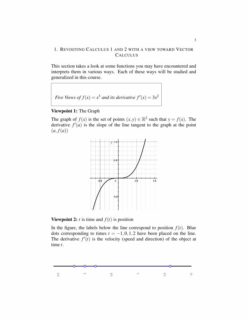
Five Views of f (x) = x3 and its derivative f ′(x) = 3x2
Viewpoint 1: The Graph
The graph of f (x) is the set of points (x,y) ∈ R2 such that y = f (x). Thederivative f ′(a) is the slope of the line tangent to the graph at the point(a, f (a))
Viewpoint 2: t is time and f (t) is position
In the figure, the labels below the line correspond to position f (t). Bluedots corresponding to times t = −1,0,1,2 have been placed on the line.The derivative f ′(t) is the velocity (speed and direction) of the object attime t.

4
Viewpoint 3: x represents position and f (x) represents temperature (oramount)
In the image, the labels below the line correspond to x and the colors cor-respond to f (x) with warmer colors representing a greater temperature (oramount) and cooler colors representing smaller temperatures (or amounts.)This is called a scalar field. The derivative f ′(x) represents the directionand amount of greatest increase in temperature.
Viewpoint 4: x is position and f (x) is a direction.
In the image, the labels below the line correspond to x and the arrows cor-respond to f (x). If f (x) < 0, the arrow points left; if f (x) > 0, the arrowpoints right. The length of the arrow corresponds to | f (x)|. The derivativef ′(x) seems to measure how much stuff is flowing into or out of x.
Viewpoint 5: x is position and f (x) is position.
In this case f is a change-of-coordinates function. Each point on the linehas two labels, we get between them by using f (or its inverse f−1(x) = 3
√x.
x −1−2 0 1 2
810−1−8f(x)
To figure out what f ′(2) (say) represents, consider the difference quotientf (2+ε)− f (2)
ε. The denominator is the length of the interval I = [2,2+ε]. The
numerator is the length of the interval obtained by applying f to the intervalI. Thus, | f (2+ε)− f (2)
ε| is the scale factor of the map f near 2. Thus, | f ′(2)|
is the infinitesimal scale factor of f at 2.

5
Two views of f (x,y) = x2 + y2
Viewpoint 1: The Graph
The graph is the set of points (x,y,z) ∈ R3 such that z = f (x,y).
The gradient
∇ f (x,y) =
(∂
∂x f (x,y)∂
∂y f (x,y)
)is the vector pointing in the direction of greatest increase in z at (x,y) ∈R2.The tangent plane to the graph of f at the point a has equation:
L(x) = ∇ f (a) · (x−a)+ f (a).
This is also the equation of the best linear (or affine) approximation to fnear a.
Viewpoint 2: Is not relevant, since the input to the function is two-dimensionaland so we shouldn’t think of it as being time.
Viewpoint 3: x is position and f (x) is temperature (or amount).

6
As with functions from R to R, this viewpoint makes sense for functionsfrom R2 to R. Below is a temperature plot of this scalar field:
-4.8 -4 -3.2 -2.4 -1.6 -0.8 0 0.8 1.6 2.4 3.2 4 4.8
-3.2
-2.4
-1.6
-0.8
0.8
1.6
2.4
3.2
The gradient ∇ f (x,y) points in the direction of greatest temperature in-crease.
Viewpoint 4: Does not make sense since the 1-dimensional output cannotexpress a direction in 2-dimensions.
Viewpoint 5: Does not make sense since the input and output to f havedifferent dimensions.
7
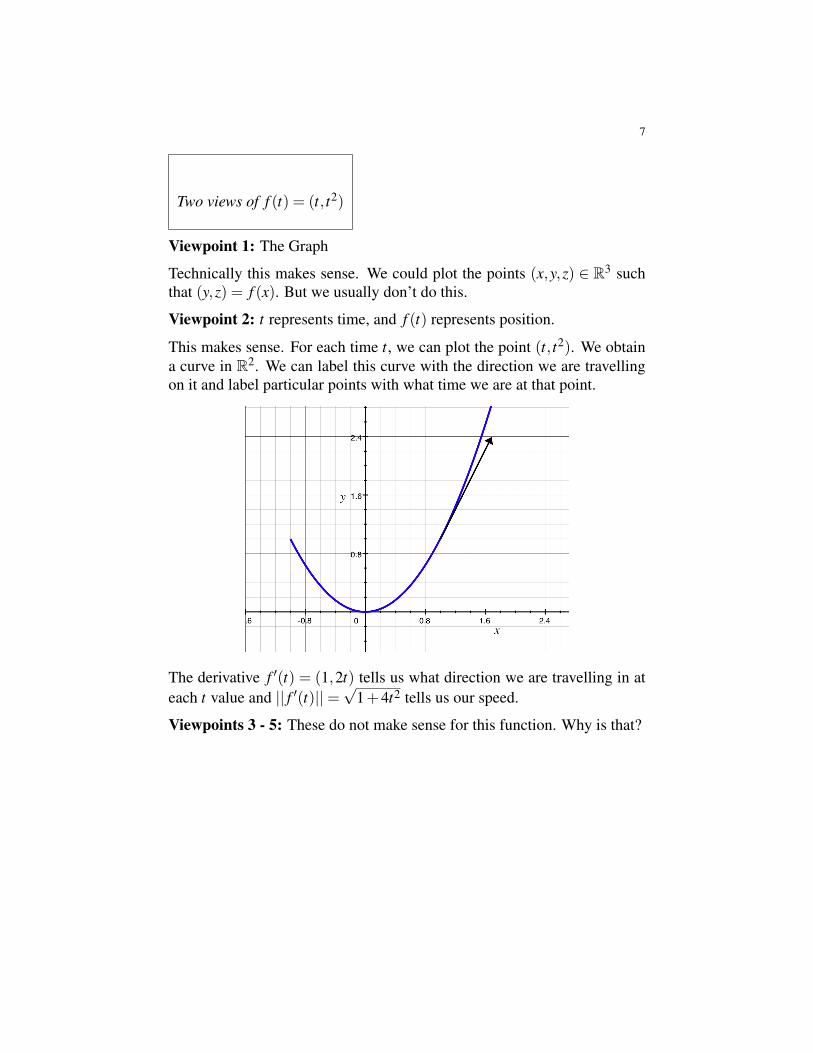
Two views of f (t) = (t, t2)
Viewpoint 1: The Graph
Technically this makes sense. We could plot the points (x,y,z) ∈ R3 suchthat (y,z) = f (x). But we usually don’t do this.
Viewpoint 2: t represents time, and f (t) represents position.
This makes sense. For each time t, we can plot the point (t, t2). We obtaina curve in R2. We can label this curve with the direction we are travellingon it and label particular points with what time we are at that point.
The derivative f ′(t) = (1,2t) tells us what direction we are travelling in ateach t value and || f ′(t)||=
√1+4t2 tells us our speed.
Viewpoints 3 - 5: These do not make sense for this function. Why is that?

8
3 Views of f (x,y) = (2x− y,x+ y)
Viewpoint 1: The Graph
Technically, this makes sense. We could plot points (x,y,z,w) ∈ R4 suchthat (z,w) = f (x,y). But we usually don’t do this.
Viewpoints 2 - 3: These don’t make sense in this context. Why is that?
Viewpoint 4: x is position and f (x) is position.
This is called a vector field. At each point (x,y) ∈ R2 we draw an arrow oflength || f (x)|| and pointing in the direction of f (x). In the computer imagebelow, the color of the arrow indicates how long it is.
Viewpoint 5: x and f (x) both represent position.
We say that f is a change of coordinates function. Under this viewpoint,each point of the plane is labelled with both x and with f (x). We think of fas a transformation taking one coordinate system to the other.
9
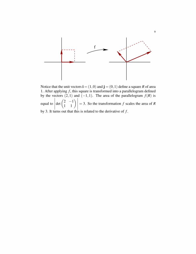
f
Notice that the unit vectors i = (1,0) and j = (0,1) define a square R of area1. After applying f , this square is transformed into a parallelogram definedby the vectors (2,1) and (−1,1). The area of the parallelogram f (R) is
equal to
∣∣∣∣∣det(
2 −11 1
)∣∣∣∣∣ = 3. So the transformation f scales the area of R
by 3. It turns out that this is related to the derivative of f .
10
2. SOME LINEAR ALGEBRA
2.1. Linear and Affine Functions. Here is the definition of linear func-tion:
Definition: A function L : Rn → Rm is linear if for all a,b ∈ Rn
and k,m ∈ R the following equation is true:
L(ka+mb) = kL(a)+mL(b.
Example 2.1. The function f (x) = 2x is linear, since:
f (ka+mb) = 2(ka+mb) = k(2a)+m(2b) = k f (a)+m f (b).
Example 2.2. The function f (x) = 2x+1 is not linear since:
f (1+1) = f (2) = 5
butf (1)+ f (1) = 3+3 = 6.
Notice that functions you may have considered to be linear in a calculuscourse will not count as linear in this course.
Example 2.3. The function h(
xy
)=
(2x− yx+ y
)is linear. To see this notice
that:
h(
k(
a1a2
)+m
(b1b2
))= h
(ka1 +mb1ka2 +mb2
)=
(2ka1 +2mb1− ka2−mb2
ka1 +mb1 + ka2 +mb2
).
Notice that this equals:
kh(
a1a2
)+mh
(b1b2
)= k(
2a1−a2a1 +a2
)+m
(2b1−b2b1 +b2
).
If you know about matrix multiplication, you should notice that, in the pre-
vious example, h(
xy
)=
(2 −11 1
)(xy
).
The following is an important theorem from linear algebra:
Theorem 2.4. A function L : Rn→ Rm is linear if and only if thereexists an m×n matrix A such that L(x) = Ax for all x ∈ Rn.
11
Definition: A function f : Rn→Rm is affine if there exists a linearfunction L : Rn→ Rm and a vector b ∈ Rm such that for all x ∈ Rn:
f (x) = L(x)+b.
That is, “affine” means “linear plus a constant”.
Equivalently, there exists an m×n matrix A and a vector b ∈ Rm such thatf (x) = Ax+b.
Example 2.5. f (x) = 2x+1 is an affine function.
Example 2.6.
f (x,y) =(
2x− y+3x+ y+1
)is an affine function since
f (x) =(
2 −11 1
)x+(
31
).
2.2. Matrix Multiplication. As you know we can write a vector a ∈Rn ineither horizontal
(a1,a2, . . . ,an)
or vertical a1a2...
an
format.
A row vector is different. It is written horizontally without commas:(a1 a2 . . . an
).
If we have a row vector a =(a1 . . . an
)and a column vector b =
b1...
bn
,
we define their product:
ab = a1b1 +a2b2 + . . .+anbn.
This should remind you of the dot product. In fact if we let aT denote thecolumn vector obtained by writing a as a column instead of as a row,
ab = aT ·b.

12
Suppose that A is an m×n matrix:
A =
a11 a12 a13 . . . a1na21 a22 a23 . . . a2n
...am1 am2 am3 . . . amn
Let a1 denote the first row, a2 the second row, etc. Write:
A =
a1a2...
am
Suppose that B is an n× p matrix:
B =
b11 b12 b13 . . . b1pb21 b22 b23 . . . b2p
...bn1 bn2 bn3 . . . bnp
Let b1 denote the first column, b2 the second column, etc. Write
B =(b1 b2 b3 . . . bp
).
Define the product of A and B to be
AB =
a1b1 a1b2 . . . a1bpa2b1 a2b2 . . . a2bp
...amb1 amb2 . . . ambp
Notice this is the m× p matrix whose entry in the ith row and jth column isthe product of the ith row of A with the jth column of B.
Example 2.7. Let A =
(2 −11 1
). Then
A(
xy
)=
(2x− yx+ y
).
Example 2.8. Let A =
(2 31 −1
). Let B =
(5 70 6
). Then
AB =
(2(5)+3(0) 2(7)+3(6)
1(5)+(−1)(0) 1(7)+(−1)(6)
)=
(10 325 1
).

13
3. DIFFERENTIATION
3.1. The derivative. We are now ready to define the derivative of a func-tion f : Rn → Rm and to define what it means to be differentiable. Theconcept is modelled on the definition from MA 122, so you should reviewthose definitions.
Definition: A function f : Rn→ Rm is differentiable at a ∈ Rn ifthere exists an affine function L : Rn→ Rm such that
• f (a) = L(a)•
limx→a
||L(x)− f (x)||||x−a||
= 0
A few remarks:
(1) The affine function L is called the “affine approximation” to f at a.The criteria ensure that the relative error between L and f goes tozero and that they are actually equal at a.
(2) In past math classes, L was probably called the “linear approxima-tion” to f , but it is, in fact, an affine function that is not necessarilylinear.
(3) Since L is an affine function, there exists an m× n matrix A suchthat L(x) = A(x−a)+ f (a). This matrix is called the derivative off at a and is denoted D f (a).
(4) If f is differentiable and if D f (x) is continuous, then we say that fis C1.
14
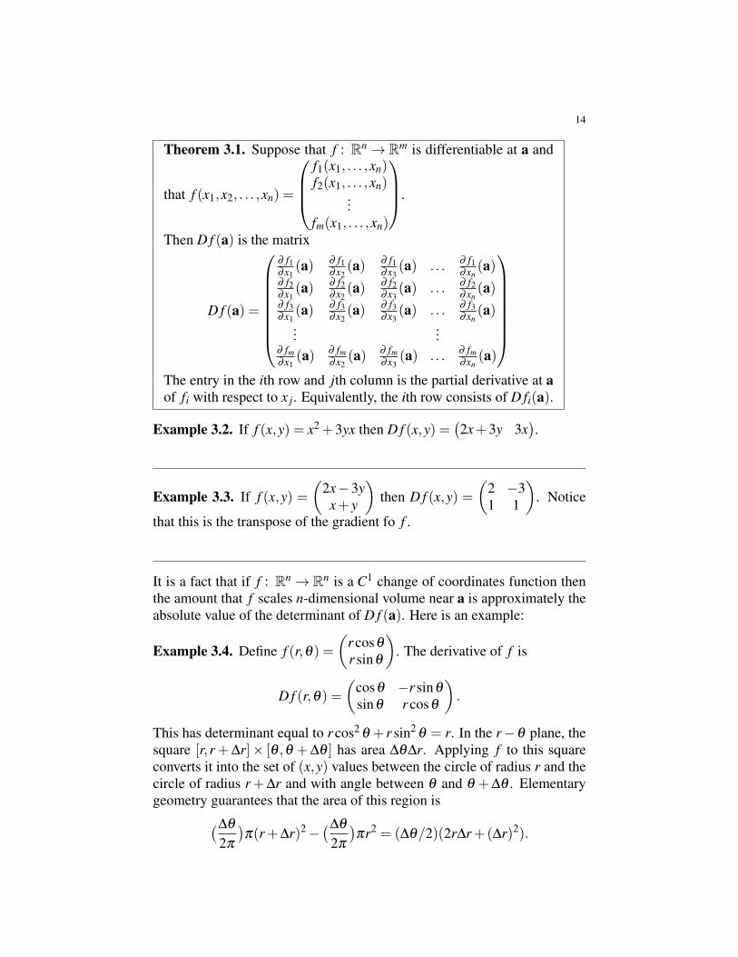
Theorem 3.1. Suppose that f : Rn→ Rm is differentiable at a and
that f (x1,x2, . . . ,xn) =
f1(x1, . . . ,xn)f2(x1, . . . ,xn)
...fm(x1, . . . ,xn)
.
Then D f (a) is the matrix
D f (a) =
∂ f1∂x1
(a) ∂ f1∂x2
(a) ∂ f1∂x3
(a) . . . ∂ f1∂xn
(a)∂ f2∂x1
(a) ∂ f2∂x2
(a) ∂ f2∂x3
(a) . . . ∂ f2∂xn
(a)∂ f3∂x1
(a) ∂ f3∂x2
(a) ∂ f3∂x3
(a) . . . ∂ f3∂xn
(a)...
...∂ fm∂x1
(a) ∂ fm∂x2
(a) ∂ fm∂x3
(a) . . . ∂ fm∂xn
(a)
The entry in the ith row and jth column is the partial derivative at aof fi with respect to x j. Equivalently, the ith row consists of D fi(a).
Example 3.2. If f (x,y) = x2 +3yx then D f (x,y) =(2x+3y 3x
).
Example 3.3. If f (x,y) =(
2x−3yx+ y
)then D f (x,y) =
(2 −31 1
). Notice
that this is the transpose of the gradient fo f .
It is a fact that if f : Rn→ Rn is a C1 change of coordinates function thenthe amount that f scales n-dimensional volume near a is approximately theabsolute value of the determinant of D f (a). Here is an example:
Example 3.4. Define f (r,θ) =(
r cosθ
r sinθ
). The derivative of f is
D f (r,θ) =(
cosθ −r sinθ
sinθ r cosθ
).
This has determinant equal to r cos2 θ + r sin2θ = r. In the r−θ plane, the
square [r,r +∆r]× [θ ,θ +∆θ ] has area ∆θ∆r. Applying f to this squareconverts it into the set of (x,y) values between the circle of radius r and thecircle of radius r+∆r and with angle between θ and θ +∆θ . Elementarygeometry guarantees that the area of this region is(∆θ
2π
)π(r+∆r)2−
(∆θ
2π
)πr2 = (∆θ/2)(2r∆r+(∆r)2).
15
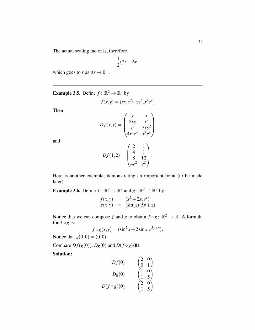
The actual scaling factor is, therefore,12(2r+∆r)
which goes to r as ∆r→ 0+.
Example 3.5. Define f : R2→ R4 by
f (x,y) = (xy,x2y,xy3,x4ey)
Then
D f (x,y) =
y x
2xy x2
y3 3xy2
4x3ey x4ey
and
D f (1,2) =
2 14 18 12
4e2 e2
.
Here is another example, demonstrating an important point (to be madelater).
Example 3.6. Define f : R2→ R2 and g : R2→ R2 by
f (x,y) = (x2 +2x,ey)g(x,y) = (sin(x),5y+ x)
Notice that we can compose f and g to obtain f ◦ g : R2→ R. A formulafor f ◦g is:
f ◦g(x,y) = (sin2 x+2sinx,e5y+x).
Notice that g(0,0) = (0,0).
Compare D f (g(0)), Dg(0) and D( f ◦g)(0).
Solution:
D f (0) =
(2 00 1
)Dg(0) =
(1 01 5
)D( f ◦g)(0) =
(2 01 5
)
16
Notice that:D( f ◦g)(0) = D f (g(0))Dg(0).
This is an example of the chain rule at work.
3.2. Differentiability.
3.2.1. Differentiability. Throughout this section, let f : Rn→ Rm be a dif-ferentiable function and let fi be the ith coordinate function. That is f (x) =( f1(x), . . . , fm(x)).
Theorem 3.7. Suppose that f : Rn→Rm has the property that eachcomponent function fi is differentiable at a. Then f is differentiableat a. Furthermore, fi : Rn→ R is differentiable at a, if there is anopen ball X containing a such that fi is defined on X and all partialderivatives of fi exist and are continuous on X .
Example 3.8. Let f : R3→ R2 be defined by
f (x,y,z) = (ln(|xyz|),x+ y+ z2)
Then
D f (x,y,z) =(
1/x 1/y 1/z1 1 2z
).
Let A be the coordinate axes in R3. That is, A = {(x,y,z) : xyz = 0}. Eachentry in the matrix D f (x,y,z) is continuous on R3− A. The function fis defined on R3−A. Consequently, f is differentiable at each point a ∈R3−A.
3.3. The chain rule. Here is the justly famous chain rule:
Theorem 3.9. Suppose that g : Rn → Rm and f : Rm → Rp arefunctions which are defined on open sets Y ⊂ Rn and X ⊂ Rm suchthat g(Y )⊂ X . Assume that g is differentiable at y ∈ Y and that f isdifferentiable at g(y)∈ X . Then, f ◦g : Rn→Rp is differentiable aty and D( f ◦g)(y) = D f
(g(y)
)Dg(y).
Example 3.10. Define f (x,y) = (x2,x2+y2). Let f : R2→R2 be the func-tion f with domain in polar coordinates. What is D f (r,θ)?
Solution: Let T : R2→R2 be the change from polar coordinates to rectan-gular coordinates. That is,
T (r,θ) = (r cosθ ,r sinθ).

17
Then, by definition, f = f ◦T . Since the coordinates of f and T are poly-nomials and trig functions, f and T are everywhere differentiable. A calcu-lation shows that:
D f (x,y) =(
2x 02x 2y
).
Thus,
D f (T (r,θ)) =(
2r cosθ 02r cosθ 2r sinθ
).
Another calculation shows that
DT (r,θ) =(
cosθ −r sinθ
sinθ r cosθ
).
Thus, by the chain rule:
D f (r,θ)=(
2r cosθ 02r cosθ 2r sinθ
)(cosθ −r sinθ
sinθ r cosθ
)=
(2r cos2 θ −2r2 cosθ sinθ
2r 0
)
The point is that “the derivative of a composition is the product of deriva-tives”.
Sketch of proof of Chain Rule. Let g : Rn→ Rm and f : Rm→ Rk be suchthat g and f are both differentiable at 0 and g(0) = 0 and f (0) = 0.
Special case: f and g are both linear.
Then there exist matrices Amk and Bnm so that
f (x) = Ax for all x ∈ Rm
g(x) = Bx for all x ∈ Rn
This implies that, for all x ∈ Rn
f ◦g(x) = A(Bx) = (AB)x.
Notice that:D f (g(0)) = A
Dg(0) = BD( f ◦g)(0) = AB
Thus,D( f ◦g)(0) = D f (g0)Dg(0)
as desired.
General Case: f and g are not necessarily linear.
18
Since g : Rn→ Rm is differentiable at 0, for x near 0,
g(x)≈ Dg(0)x.
Similarly, since f : Rm→ Rk is differentiable at g(0) = 0, for x near 0,
f (x)≈ D f (g(0))x.
To prove the theorem we just need to show that
f ◦g(x)≈ D f (g(0))Dg(0).Remember that ≈ in this context means that the relative error goes to 0 asx→ 0. We didn’t go over this in class, but here is a proof:
For convenience, define the following:
B = Dg(0)A = D f (0)
We need to show that for each ε > 0, there exists δ > 0 so that if 0 < ||x||=||x−0||< δ then
|| f ◦g(x)−ABx||||x−0||
< ε.
Notice that:
|| f ◦g(x)−ABx||= || f ◦g(x)−Ag(x)+Ag(x)−ABx||.By the triangle inequality,
|| f ◦g(x)−ABx|| ≤ || f ◦g(x)−Ag(x)||+ ||A(gx)−Bx)||.
Now there exists a constant α , such that for all y ∈ Rm, ||Ay|| ≤ α||y||.Thus,
|| f ◦g(x)−ABx|| ≤|| f (g(x))−Ag(x)||+ ||A(gx)−Bx)|| ≤|| f (g(x))−Ag(x)||+α||g(x−Bx||
We now consider the relative errors.
Piece 1: Since g is differentiable at 0, there exists δ1 > 0, so that if 0 <||x||< δ1 then
||g(x)−Bx||||x||
< ε/2α.
Piece 2: There is a theorem, which guarantees that (since g is differentiableat 0) there exists δ2 > 0 so that if ||x||< δ2, then there is a constant β suchthat
||g(x)|| ≤ β ||x||.
19
Piece 3: Since f is differentiable at 0 = g(0), there exists δ3 > 0 so that if0 < ||y||< δ3, then
|| f (y)−Ay||y||
< ε/2β .
This implies that|| f (y)−Ay||< (ε/2β )||y||
Pieces 2 and 3 imply: if 0 < x < min(δ2,δ3), setting y = g(x) we have
|| f (g(x)−Ag(x)||< (ε/2β )||g(x)||< (ε/2β )β ||x||.
Consequently, if 0 < x < min(δ2,δ3), we have|| f (g(x))−Ag(x)
||x||< ε/2.
Piece 1 implies: if 0 < x < δ1, thenα||g(x)−Bx||
||x||< ε/2.
We conclude that if 0 < ||x||< δ = min(δ1,δ2,δ3) then
|| f ◦g(x)−ABx||/||x|| ≤|| f (g(x))−Ag(x)||/||x||+α||g(x)−Bx||/||x|| <
ε/2+ ε/2 = ε
as desired. �

20
4. PARAMETERIZED CURVES
A function x : R→ Rn traces out a path in Rn. The set of points
{a ∈ Rn : x(t) = a for some t ∈ R}is called the image of the path x. If x is one-to-one (so that no place on theimage occurs at more than one time) we say that x is a parameterizationof its image. We also allow the domain to be a subset of R rather than all ofR.
4.1. Some important examples.
Example 4.1. The path x1(t) =(
cos tsin t
)for t ∈ [0,2π] is a parameteriza-
tion of the unit circle inR2. The path x2(t) =(
cos2tsin2t
)for t ∈ [0,2π] also
has image the unit circle but is not a parameterization of it since it travels
through each point on the unit circle twice. The path x3(t) =(
cos2tsin2t
)for
t ∈ [0,π] is parameterization of the unit circle. The path x3 is different fromthe path x1 since it travels around the circle twice as fast.
Example 4.2. The path x(t) =
cos tsin t
t
is a parameterization of a helix in
R3 that winds around the z-axis.

21
Example 4.3. Suppose that f : R → R is a continuous function. Thenx(t) = (t, f (t)) is a parameterization of the graph of f in R2. The pathy(t) = (−t, f (−t)) is a parameterization of the graph that travels in the op-posite direction.
Example 4.4. Suppose that v and w are distinct vectors in Rn. Then x(t) =tv+(1− t)w is a parameterization of the line through v and w. Restrictingx to t ∈ [0,1] is a parametrization of the line segment joining v and w.
Example 4.5. Suppose that v and w are distinct vectors in Rn. Then x(t) =v+tw is a parameterization of the line through v that is parallel to the vectorw.
4.2. Velocity and Acceleration. If x : R→ Rn is a differentiable param-eterized curve, its velocity is x′(t) = Dx(t) and its acceleration is v′(t) =Dv(t). The speed of x is ||x′(t)||.
Example 4.6. Find v(t) and a(t) for the curve x(t) = (t, t sin(t), t cos(t)).Also find the speed of x(t) at time t.
Solution:
v(t) = (1,sin(t)+ t cos(t),cos(t)− t sin(t))
||v(t)|| =√
1+ sin(t)cos(t)− t2 sin(t)cos(t)− t sin2(t)+ t cos2(t)a(t) = (0,2cos(t)− t sin(t),−2sin(t)− t cos(t))
The next theorem should not be surprising.
Theorem 4.7. Suppose that x : R→ Rn is differentiable. Then x′(t0) isparallel to the line tangent to the curve x(t) at t0.
Proof. We consider only n = 2; for n > 2, the proof is nearly identical. Avector parallel to the tangent line to x(t) at t = t0 can be obtained as in

22
1-variable calculus:
tangent vector = lim∆t→0(x(t0 +∆t)−x(t0)
)/∆t
= lim∆t→0
((x(t0 +∆t),y(t0 +∆t)
)−(x(t0),y(t0)
))/∆t
= lim∆t→0
(x(t0+∆t)−x(t0)
∆t , y(t0+∆t)−y(t0)∆t
)=
(lim∆t→0
x(t0+∆t)−x(t0)∆t , lim∆t→0
y(t0+∆t)−y(t0)∆t
)= (x′(t),y′(t))= x′(t)
�
Example 4.8. Let x(t)= (3cos(2t),sin(6t)). The image of x for t ∈ [−6π,6π]is drawn below. Find the equations of the tangent lines at the point (−1.5,0).
Solution: The point (−1.5,0) is crossed by x at t1 = π/3 and at t2 = 2π/3.The derivative of x is
x′(t) = (−6sin(2t),6cos(6t)).
At t1, we have:
x′(t1) = (−6sin(2π/3),6cos(2π)) = (−3√
3,6).
Thus, one of the tangent lines has parameterization:
L1(t) = t(−3√
3,6)+(−1.5,0).
At t2, we have:
x′(t2) = (3√
3,6).
Thus, the other tangent line has a parameterization:
L2(t) = t(3√
3,6)+(−1.5,0).

23
4.3. Tangent space coordinates. In the previous section we saw that if xwas a parameterized curve, then x′(t) is a vector parallel to the tangent lineto the image of x at t. It would be much better to base our derivative vectorat the point x(t). We can do this if we change coordinate systems.
Here is the idea:
Example 4.9. Let x(t) = (cos t,sin t) and let t0 = (π/4,π/4). Notice thatx′(t0) = (1/
√2,1/√
2). If an object’s position at time t seconds is givenby x(t) and if at time t0 all forces stop acting on the object then 1 secondlater, the object will be at the position given by x(t0) + x′(t0). That is,x′(t0) denotes the direction the object will travel starting at x(t0). It wouldbe convenient to represent x(t0) by a vector with tail at x(t0) and head atx(t0)+x′(t0).
FIGURE 1
To do this to each point p ∈ Rn we associate a “tangent space” Tp. This issimply a copy of Rn such that p corresponds to the origin of Tp. In R2, thestandard basis vectors are denoted i and j. In R3 the standard basis vectorsare denoted i, j, and k. We usually think of Tp as an alternative coordinatesystem for Rn which is positioned so that p ∈ Rn is at the origin.
Example 4.10. If p = (1,3) and if (2,5) ∈ Tp then (2,5) corresponds to thepoint (1,3)+(2,5) = (3,8) in R2.
We think of Tp as the set of directions at p.
Example 4.11. Let x(t) = (cos t,sin t) and let t0 = π/6. Suppose that anobject is following the path x(t) and that at time t0 all forces stop acting on
24
the object. Then the direction in which the object will head is
x′(t0) = (−sinπ/6,cosπ/6) = (−1/2,√
3/2).
That is, the object will travel 1/2 units to the left of x(t0) and√
3/2 unitsup from x(t0) in 1 second.
Put another way, the point x(t0)+ x′(t0) is the same as the point x′(t0) ∈Tx(t0).
Suppose that f : Rn→ Rm is differentiable at p ∈ Rn. Then L : Tp→ Tf (p)defined by
L(x) = D f (p)xis a linear map between tangent spaces.
Example 4.12. Let p = (1,2) ∈ R2 and let f (x) = (1/4)(x2 + y2,x2− y2)for all x = (x,y). Let v = (−2,3) ∈ Tp. Sketch the point D f (p)v ∈ Tf (p).
Solution: Compute:
D f (x,y) =(
x/2 y/2x/2 −y/2
).
So that
D f (p) =(
1/2 11/2 −1
).
Thus,
D f (p)v =
(1/2 11/2 −1
)(−23
)=
(2−4
).
In R2, we plot D f (p)v by starting at f (p) = (5/4,−3/4) and then travelover 2 and down 4. See Figure 2.

25
FIGURE 2. On the left is an arrow representing v ∈ Tp. Onthe right is an arrow representing D f (p)v in Tf (p).
Example 4.13. Suppose that a circle of radius ρ cm rolls along level groundso that the center of the circle is moving at 1 cm/sec. At time t = 0, thecenter of the circle is at (0,0) and the top of the circle is a point P = (0,ρ).As the circle rolls, the point P traces out a curve x(t) (with P = x(0)). Findan equation for x(t).
Solution: Let c(t) denote the center of the circle at time t. The circumfer-ence of the circle is 2πρ and so the circle makes one complete rotation in2πρ sec. At time t, the line segment joining c(t) to x(t) makes an angle of−t/ρ +π/2 with the horizontal. That is, in Tc(t), x(t) is represented by thepoint (ρ cos(−t/ρ + π/2),ρ sin(−t/ρ + π/2)). Thus, with respect to thestandard coordinates on R2:
x(t) = c(t)+(
ρ cos(−t/ρ +π/2)ρ sin(−t/ρ +π/2)
).
Since
c(t) = t(
10
),
we have
x(t) =(
t +ρ cos(−t/ρ +π/2)ρ sin(−t/ρ +π/2)
).

26
Question: Is the cycloid a differentiable curve?
Example 4.14. Suppose that a circle C of radius r is moving so that thecenter of C, c traces out the path (Rcos(t),Rsin(t)). As C moves, it rotatescounterclockwise so that it completes k revolutions per second. Supposethat E is the East pole of C at time 0. What path does P trace out?
Solution: In Tc(t), E has coordinates (r cos2πkt,r sin2πkt). Thus in R2
coordinates, E has position
x(t) = c(t)+(r cos t,r sin t) = (Rcos t + r cos2πkt,Rsin t + r sin2πkt).
4.4. Intrinsic vs. Extrinsic.
Example 4.15. Consider the parameterizations
x(t) =(
cos tsin t
)for 0≤ t ≤ 2π

27
and
y(t) =(
cos2tsin2t
)for 0≤ t ≤ π.
Both are parameterizations of the unit circle. To use either of them to studythe unit circle we need to develop properties of parameterizations that de-pend only on the underlying curve and not on the parameterization chosen.Such properties are called “intrinsic” properties of the curve.
Definition 4.16. A function h : [c,d]→ [a,b] is a change of coordinatesfunction if it is a C1 bijection. Often we will also require h to have theproperty that for all t, h′(t) 6= 0.
(Recall: C1 means that its derivative always exists and is continuous. A“bijection” is a function that is both one-to-one and onto.)
Example 4.17. Define h(t) : [0,π]→ [0,2π] by h(t) = 2t. The function his a change of coordinates function.
Example 4.18. Define h : [0,1]→ [0,1] by h(t) = t3. Then h is a change ofcoordinates function, but its inverse h−1(t) = 3
√t is not a change of coordi-
nates function because it is not differentiable at t = 0.
Example 4.19. Find a change of coordinates function h : [0,1] → [0,1]such that h(0) = 1 and h(1) = 0. (This is an example of an “orientation-reversing” change of coordinates function.
Solution: Sketch the x and y axes. Any function that is monotonicallydecreasing from the point (0,1) to the point (1,0) will work. The functionh(t) =−t +1 is one such function.
Notice that if h is a change of coordinates function with h′(t) 6= 0 for any t,then either h′(t)> 0 for all t or h′(t)< 0 for all t (by the intermediate valuetheorem).
Definition 4.20. A change of coordinates function h : [c,d]→ [a,b] is orientation-preserving if h′(t)> 0 for all t and is orientation-reversing if h′(t)< 0 forall t. Notice that if h is orientation-preserving then h(c) = a and h(d) = bwhile if h is orientation-reversing then h(c) = b and h(d) = a.
28
Definition 4.21. If x : [a,b]→Rn and y : [c,d]→Rn are paths, we say thaty is a reparameterization of x if there exists a change of coordinates func-tion h : [c,d]→ [a,b] such that y = x◦h. If h is orientation preserving, wesay that y is an orientation-preserving reparameterization of x. If h isorientation reversing, we say that y is an orientation-reversing reparame-terization of x.
The key point is that: reparameterizing a curve is changing the speed andpossibly the direction that we walk along the curve. Intuitively, the change-of-coordinates function h tells us how to speed up or slow down as wetraverse that path laid down by x. If y is an orientation-preserving repa-rameterization of x, it traces out the path in the same direction that x did,otherwise it traces the path out in the opposite direction.
Example 4.22. Let x(t) =(
t2
2t
)for t ∈ [0,5]. Let y(t) =
(9t2
6t
)for t ∈
[0,5/3].
The path y is an orientation reparameterization of x by the change of coor-dinates function h(t) = 3t.
Example 4.23. Let x(t)= (cos t,sin t) for t ∈ [0,2π] and let y(t)= (cos3t,sin3t)for t ∈ [0,2π]. Then y is not a reparameterization of x since x traverses theunit circle once, but y traverses it three times.
Example 4.24. Let x(t) =
tcos tsin t
for t ∈ [π,2π]. Let y(t) =
t3
cos t3
sin t3
for t ∈ [ 3
√π, 3√
2π].
The path y is an orientation-preserving reparameterization of x using thechange of coordinates function h(t) = t3 for t ∈ [ 3
√π, 3√
2π].
Example 4.25. Let G be the graph of a function y = f (x) for x∈ [a,b]. Findtwo parameterizations, with opposite orientations, of G.
One parameterization is x(t) =(
tf (t)
)for t ∈ [a,b]. A second one is
y(t) =(−t
f (−t)
)for t ∈ [−b,−a]. Since they are related by the change

29
of coordinates function h(t) = −t which has h′(t) = −1, the curves havethe opposite orientations.
Definition 4.26. A quantity is intrinsic if it does not change under orien-tation preserving reparameterization. A quantity is intrinsic to orientedcurves if it does not change under orientation preserving reparameteriza-tion.
Example 4.27. If x : [a,b]→ Rn is a path, its derivative and speed are notintrinsic, since we can walk the same path at a different speed.
Example 4.28. Let x : [a,b]→ Rn be a C1 path such that ||x′(t)|| 6= 0 forany t. Then the unit tangent vector
Tx(t) =x′
||x′||is intrinsic to the oriented curve.
To see this, suppose that y : [c,d]→Rn is another C1 path such that ||y′(t)|| 6=0 for any t and suppose that h : [c,d]→ [a,b] is an orientation preserv-ing change of coordinate function so that y = x ◦ h. We need to show thatTy(t) = Tx(h(t)) for all t.
By the chain rule,y′(t) = x′(h(t))h′(t).
Notice that since h is orientation preserving, h′(t) = |h′(t)| for all t. Thus,
Ty(t) = y′(t)||y′(t)||
= x′(h(t))h′(t)||x′(h(t))h′(t)||
= x′(h(t))h′(t)||x′(h(t))|| |h′(t)|
= x′(h(t))h′(t)||x′(h(t))||h′(t)
= x′(h(t))||x′(h(t))
= Tx(t)
30
Example 4.29. Here is an informal example that we will develop in the nextsection.
If x : [a,b]→ Rn is a curve that, as a function, is one-to-one, we can defineits length to be the limit of the lengths of piecewise linear approximationsto the image of x. Since this does not depend on the parameterization thislength that we calculate is intrinsic to x.

31
4.5. Arc length. Suppose that x : [a,b]→R is a C1 curve. We wish to findthe length of x. The formula is
Theorem 4.30. The arc length of x is∫ b
a||x′(t)||dt.
Arc length is often denote by ∫x
ds
whereds = ||x′||dt
Example 4.31. Let x(t) = (t2,2t2) for t ∈ [0,1]. Then
||x′(t)||= ||(2t,4t)||=√
4t2 +16t2 = 2t√
5.
The arclength of x is∫x
ds =∫ 1
02t√
5dt = t2√
5∣∣10 =√
5.
Example 4.32. Let x(t) = (t, t2) for t ∈ [0,1]. Then∫x
ds =∫ 1
0
√1+4t2 dt ≈ 1.47894
Here is why the formula for arclength is what it is. For convenience, weassume that n = 2.
Partition [a,b] into n subintervals [ti−1, ti] for 1≤ i≤ n, each of length ∆t =(b− a)/n. Joining the points x(ti−1) and x(ti) by straight lines creates apolygonal approximation Pn to the image of x. The length of the polygonalpath is:
length(Pn) =n
∑i=1||x(ti)−x(ti−1)||.
We define the arc length of x to be
L =∫
xds = lim
n→∞
n
∑i=1||x(ti)−x(ti−1)||.
Now suppose that x(t) = (x(t),y(t)). Both x and y are C1 functions. Noticethat if we replace our current polygonal approximation with a polygonalapproximation have vertices (x(t∗i ),y(t
∗∗i )), with t∗i , t
∗∗i ∈ [ti−1, ti], we will
32
still have:
L =∫
xds = lim
n→∞
n
∑i=1||(x(t∗i ),y(t∗∗i ))− (x(t∗i−1),y(t
∗∗i−1))||.
Here’s how to choose the values t∗i and t∗∗i . By the mean value theorem(remember that?) There exists t∗i , t
∗∗i ∈ [ti−1, ti] so that
x(t∗i ) = x′(t∗i )(ti− ti−1) = x′(t∗i )∆ty(t∗∗i ) = y′(t∗∗i )(ti− ti−1) = y′(t∗∗i )∆t
Thus,
L= limn→∞
n
∑i=1
√(x′(t∗i )2 + y′(t∗∗i )2∆t =
∫ b
a
√x′(t)2 + y′(t)2 dt =
∫ b
a||x′(t)||dt.
We can also compute the arc length of paths which are piecewise C1. Thesepaths must be composed of a finite number of pieces.
Example 4.33. Compute the length of the curve x : [0,2]→ R defined by:
x(t) ={
(t, t2) if 0≤ t ≤ 1(t,(2− t)2) if 1≤ t ≤ 2
}
Solution: Let x1(t) = x(t) for 0≤ t ≤ 1 and let x2(t) = x(t) for 1≤ t ≤ 2.Then ∫
x ds =∫
x1ds+
∫x2
ds=
∫ 10
√1+4t2 dt +
∫ 21
√1+4(2− t)2
≈ 2.95789
The following example shows that it is possible for a “finite” curve to haveinfinite length.
Example 4.34. We will specify the graph of the curve f (x). On the interval[ 1
n+2 ,1n ] erect a tent consisting of two straight lines with the bottoms of the
lines on the x axis and the top of the tent at the point ( 1n+1 ,
1n). See the figure
below:
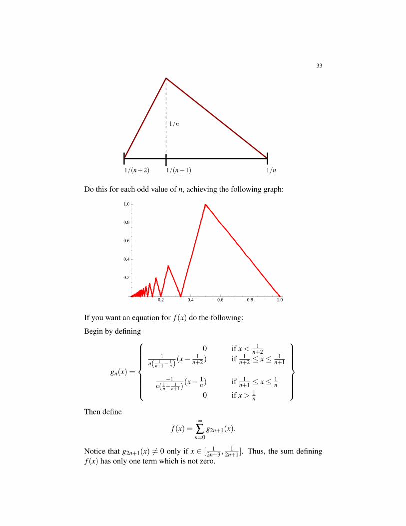
33
1/n
1/n1/(n+1)1/(n+2)
Do this for each odd value of n, achieving the following graph:
0.2 0.4 0.6 0.8 1.0
0.2
0.4
0.6
0.8
1.0
If you want an equation for f (x) do the following:
Begin by defining
gn(x) =
0 if x < 1n+2
1n( 1
n+1−1n)(x− 1
n+2) if 1n+2 ≤ x≤ 1
n+1
−1n( 1
n−1
n+1)(x− 1
n) if 1n+1 ≤ x≤ 1
n
0 if x > 1n
Then define
f (x) =∞
∑n=0
g2n+1(x).
Notice that g2n+1(x) 6= 0 only if x ∈ [ 12n+3 ,
12n+1 ]. Thus, the sum defining
f (x) has only one term which is not zero.

34
Let’s show that the length of the graph of f is infinite. To do this, considerthe line segment in the interval [ 1
n+1 ,1n ] for an odd value of n. This line
segment has length
L =
√(1n)2 +(
1n− 1
n+1)2 =
√2n2 +
1(n+1)2 −
2n(n+1)
.
Some algebra shows that L ≥ 1n Similarly, the line segment in the interval
[ 1n+2 ,
1n+1 ] has length at least 1/(n+ 1). Consequently, the length of the
graph of f is at least∞
∑n=1
1n.
It is well known that this is the harmonic series which diverges to infinity.
The text gives an example of a function f : [0,1]→ [−1,1] which is dif-ferentiable on (0,1] but whose graph has infinite arclength. An examplesimilar to that one could be constructed from our example by rounding thepoints of the graph above.
Theorem 4.35 (Arc length is intrinsic). Suppose that x : [a,b]→ Rn andy : [c,d]→ Rn are C1 curves and that y is a reparameterization of x. Thenthe length of y is equal to the length of x.
Proof. Since y is a reparameterization of x, there exists a change-of-coordinatesfunction h : [c,d]→ [a,b] such that y = x◦h. By the chain rule we have:
y′(t) = x′(h(t))h′(t).
Taking magnitudes gives:
||y′(t)||= ||x′(h(t))|| |h′(t)|.Case 1: h is orientation-preserving. In this case, |h′(t)| = h′(t). Then, bydefinition, the length of y is:
L(y) =∫ d
c ||y′(t)||dt=
∫ dc ||x′(t)||h′(t)dt.
Let u = h(t). Then du = h′(t)dt and u(c) = a and u(d) = b since h isorientation preserving. Thus, substitution shows that:∫ d
c||x′(t)||h′(t)dt =
∫ b
a||x(u)||du.
This latter integral is exactly the length of x.
Case 2: h is orientation-reversing.

35
This case is left to the reader. It follows from the observations that |h′(t)|=−h′(t) and h(c) = b and h(d) = a. �
Being able to calculate arclength is not just an end-in-itself. It also givesus a useful way of reparameterizing so that we always travel at unit speed(eg. 1 meter/sec.) This reparameterization is called reparameterizationby arclength. If a curve x : [a,b] → Rn has the property that for all t,||x′(t)|| = 1, we say that x is parameterized by arclength. Here’s how todo it:
Suppose that x : [a,b] → R is C1 and that ||x′(t)|| > 0 for all t ∈ [a,b].Define s : [a,b]→ [0,L] by
s(t) =∫ t
a||x′(τ)||dτ.
Notice that s is a strictly increasing C1 function and so is an orientation pre-serving bijection [a,b]→ [0,L]. By the fundamental theorem of Calculus,s′(t) = ||x′(t)|| so we often write ds = ||x′(t)||dt.
Furthermore, its inverse function s−1 : [a,b]→ [a,L] is also strictly increas-ing bijection. Define y(t) = x ◦ s−1. The function s measures the distancetravelled from time a to time t using the path x. Composing x with s−1
makes it so that x travels at one unit of distance per unit of time. (Like howdriving at 60 mph means that you travel at 1 mile per minute.)
For the record: How to reparameterize by arclength, given x : [a,b]→Rn
such that ||x′(t)|| 6= 0.
(1) Find s : [a,b]→ [0,L] defined by
s(t) =∫ t
a||x′(τ)||dτ.
(2) Find the inverse function s−1 : [0,L]→ [a,b]. Do this by settingσ = s(t) and solving for t.
(3) Define y(σ) = x(s−1(σ)). That is, y = x ◦ s−1. The curve y isthe reparameterization of x by arclength, as we show after someexamples.
Example 4.36. Reparameterizing x(t) =(
t3t
)for t ∈ [0,2] by arclength.
Solution: Notice that ||x′(t)||=√
10. Thus,
s(t) =∫ t
0
√10dτ =
√10t.

36
Let σ =√
10t and solve for t to find that:
s−1(σ) = t = σ/√
10.
Thus,
y(σ) = x(s−1(σ)) =
(σ/√
103σ/√
10
)is a reparameterization of x by arclength.
Example 4.37. Let x(t) =
tt
(2/3)t3/2
for t ∈ [1,10]. Reparameterize x
by arclength.
Solution: Notice that x′(t) = (1,1, t1/2) and that ||x′(t)||=√
2+ t. Thus,
σ = s(t) =∫ t
1
√2+ τ dτ = (2/3)(2+ t)3/2.
Solving for t we get:
s−1(σ) = t = (3σ/2)2/3−2.
We plug into x to get:
y(σ) = x(s−1(σ) =
(3σ/2)2/3−2(3σ/32)2/3−2
(2/3)((3σ/2)3/2−2)(3/2)
.
Next we prove that the steps to reparameterization work, and then we dosome other examples.
Lemma 4.38. Assume that x is a C1 curve defined on [a,b] such that for allt, ||x′(t)|| 6= 0. Let y be the reparameterization of x by arc length. Then forall t, ||y′(t)||= 1 and the length of y on the interval [0, t] is t.
Proof. Notice that:s′(t) = ||x′(t)||
by the fundamental theorem of Calculus. Also, y = x◦ s−1 means that x =y◦ s. Consequently, by the chain rule,
||x′(t)||= ||y′(s(t))|| |s′(t)|
37
Letting σ = s(t) and recalling that s′(t) = ||x′(t)|| we get:
||x′(t)||= ||y′(σ)|| ||x′(t)||.
Thus, since ||x′(t)|| 6= 0,||y′(σ)||= 1.
The length of y on the interval [0, t] is, by definition,∫ t
0||y′(σ)||dσ .
We see immediately that this equals t. �
Example 4.39. Let x(t) = (t2,3t2) for t ∈ [1,2]. Reparameterize x by arclength.
Answer: By definition,
s(t) =∫ t
1
√4τ2 +36τ2 dτ
=∫ t
1√
40τ dτ
=√
40(t2−1)
We need, s−1. Solving the previous equation for t we find:
t =√
1+ s/√
40
Thus,
s−1(t) =√
1+ t/√
40
To get y(t) which is the reparameterization of x by arclength, we plug thisin for t in the equation for x, getting:
y(t) = x◦ s−1(t)
=((√
1+ t/√
40)2
,3(√
1+ t/√
40)2 )
=(1+ t/
√40,3(1+ t/
√40))
To avoid much of this algebra, we will often simply write x(s) instead ofx◦s−1. This notation has the potential to be confusing. Thus, in the previousexample, the reparameterization of x(t) = (t2,3t2) by arc length is
x(s) =(1+ s/
√40,3(1+ s/
√40)).
Example 4.40. Let x(t) = (cos t,sin t,(2/3)t3/2) for t ≥ 3. Find x(s).
Answer: Compute:
||x′(t)||= ||(−sin t,cos t, t1/2)||=√
1+ t.

38
Thus,
s=∫ t
3
√1+ τ dτ =(2/3)(1+t)3/2−(2/3)(1+3)3/2 =(2/3)(1+t)3/2−16/3.
Consequently,
t =(
3(s+16/3)2
)2/3
Thus,
x(s)=
(cos(
3(s+16/3)2
)2/3
,sin(
3(s+16/3)2
)2/3
,(2/3)(
3(s+16/3)2
)4/3)
4.6. Curvature and the Moving Frame. In this section we assign an in-trinsic tangent space coordinate system to each point x on the image of apath x : [a,b]→ R3 called the moving frame.
We begin with an important lemma. It can be interpreted as saying that if apath lies on a sphere then its position vector is perpendicular to its tangentvector. This should not be a surprise if we believe that the radius of a circleis perpendicular to the tangent line intersecting it.
Lemma 4.41. Suppose that φ : [a,b]→Rn is a C1 path such that ||φ(t)|| isconstant. Then, for all t, φ(t) is perpendicular to φ ′(t).
Proof. Since ||φ(t)|| is constant,
φ(t) ·φ(t) = ||φ(t)||
is constant. Thus,ddt
φ(t) ·φ(t) = 0.
By the product rule we have:
φ′(t) ·φ(t)+φ(t) ·φ ′(t) = 0.
Since dot product is commutative, this implies that
2φ(t) ·φ ′(t) = 0.
Consequently,φ(t) ·φ ′(t) = 0
as desired. �
We already know that the unit tangent vector T is intrinsice to an orientedcurve, so we take it as one of our coordinate directions in our moving frame.

39
By the previous lemma, its derivative T′ is perpendicular to it. So we definethe unit normal vector to be
N(t) =T′(t)||T′(t)||
.
Our third coordinate direction needs to be of unit length and perpendicularto both T and B. We call it the unit binormal vector:
B(t) = T(t)×N(t).
Using the unit tangent vector we can also define the curvature of a curve xto be:
κ(t) =||T′(t)||||x′(t)||
.
Example 4.42. Find the curvature of a line x(t) = tv+b.
Answer: We haveT = x′/||x||= v/||v||.
Thus, dT/dt = 0 and so κ(t) = 0.
Example 4.43. The curvature of a circle of radius r > 0 is 1/r at each pointon the circle.
Example 4.44. Let φ(t) = (t,at2) be a parameterized curve. Find the cur-vature of φ at t = 0.
Answer: We have: φ ′(t) = (1,2at) and T = (1,2at)/√
1+4a2t2. Thus,
ddt
T = (0,2a)/√
1+4a2t2 +(1,2at)(−1/2)(1+4a2t2)−3/2(8a2t).
Thus,||φ ′(0)||= 1
and
|| ddt
T(0)||= ||(0,2a)||= 2a
Consequently,κ(t) = 2a/1 = 2a

40
Example 4.45. Compute the moving frame and curvature for the path x(t)=(sin t− t cos t,cos t + t sin t,2) with t ≥ 0.
Answer: We compute:
x′(t) = (cos t− cos t + t sin t,−sin t + sin t + t cos t,0) = (t sin t, t cos t,0)
||x′(t)|| =√
t2 sin2 t + t2 cos2 t = t
T = x′(t)/||x′(t)|| = (sin t,cos t,0)
T′ = (−cos t,sin t,0)
||T′|| = 1
N = T′/||T′|| = (−cos t,sin t,0)
κ = ||T′||/||x′|| = 1/t
Finally, to compute B we need the cross product:
B = (sin t,cos t,0)× (−cos t,sin t,0) = (0,0,1).
It turns out thatB′(t)||x′(t)||
=−τN
for some scalar function τ , called the torsion. If τ(t) = 0 for all t, theBinormal vector is constant and so is the plane perpendicular to it. Thatplane contains x and so the torsion measures how much the curve twists outof a plane. If τ(t) = 0 for all t, then the curve lies in a plane.
Example 4.46. Let x(t) =
sin t− t cos tcos t + t sin t
t2
for t > 0. Calculate T, N, B, κ ,
and τ for x.
Easy computations show that:
x′(t) =
t sin tt cos t
2t
||x′(t)|| = t
√5.
41
More computations show:
T(t) = 1√5
sin tcos t
2
T′(t) = 1√5
cos t−sin t
0
N(t) =
cos t−sin t
0
κ(t) = 1
5t
B(t) = 1√5
2sin t2cos t−1
B′(t) = 1√5
2cos t−2sin t
0
B′(t)/||x′(t)|| = 2
5t N(t)
τ(t) = − 25t .
.

42
5. INTEGRATING VECTOR FIELDS AND SCALAR FIELDS OVER CURVES
Warm-up Question 1: Suppose that a constant force of f Newtons pushesa box d meters. How much work was done?
Answer: d f Newton-meters of work was done, since if a force is constantand in the direction of motion, then the work done is equal to the magnitudeof the force times the distance moved.
Warm-up Question 2:Suppose that a constant force of f Newtons is ap-plied to a box and moves the box d meters. This time, however, the force isat an angle of θ degress with the direction of motion. How much work isdone by the force?
Solution: Let F be the force and let d be the direction. The projection of Fonto d tells us how much of the force is in the direction of motion. Sometrigonometry tells us that it is ||F||cosθ . Taking this times the distancetravelled gives:
Work done = ||F||||d||cosθ = F ·d.
Warm-up Question 3: Suppose that at each point on a path x : [a,b]→Rn
there is a different force F. Assume that the path and the function F are C1.How much work is done by the force to an object moving along the path?
Solution: Break the path into segments of equal length ∆s and pretend thatF is constant on each segment and that the image of x is a polygonal pathwith endpoints corresponding to the segment breaks. We would then add upF ·d on each segment. This gives an approximation to the work done. If wewant the exact value we take a limit. This suggests defining the work doneto be: ∫ b
aF(x(t)) ·x′(t)dt.
This last integral is an example of a path integral of a vector field. Beforediscussing them more, we discuss path integrals of scalar fields.
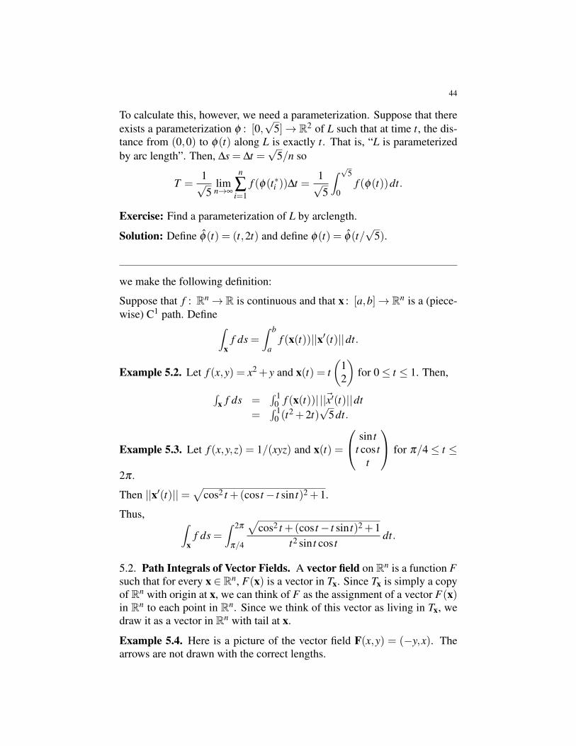
5.1. Path Integrals of Scalar Fields. A scalar field on Rn is simply afunction f : Rn → R. We think of f as assigning a number f (x) to eachpoint x in Rn. Below is a depiction of the scalar field f (x,y) = x2 + y2 onR2. To a point (x,y) ∈ R2, we assign the number x2 + y2. Points whichare assigned small numbers are colored blue and points which are assignedlarge numbers are colored red.

43
-40 -35 -30 -25 -20 -15 -10 -5 0 5 10 15 20 25 30 35 40
-25
-20
-15
-10
-5
5
10
15
20
25
The following example demonstrates the important idea of integrating ascalar field over a curve.
Example 5.1. Let L be a straight piece of wire in R2 with endpoints at(0,0) and at (1,2). Suppose that the temperature of the wire at point (x,y)is f (x,y) = x2 + y. Find the average temperature of the wire.
Solution: Break the wire L into little tiny segments, L1, . . . ,Ln each oflength ∆s. Since L has a length of
√5, ∆s =
√5/n.
Then the average temperature of L is approximately
Tn =1n
n
∑i=1
f (x∗i )
In fact, the average temperature of L is exactly
T = limn→∞
1n
n
∑i=1
f (x∗i ).
Recall that 1/n = (∆s)/√
5. Thus,
T = limn→∞
1√5
n
∑i=1
f (x∗i )∆s
This looks a lot like a limit of Riemann sums, so perhaps we can convertthis to a definite integral and use the Fundamental Theorem of Calculus.Before we do that, however, notice that (up to proving that the limit exists)we have a perfectly fine definition of the quantity
Ave. value of f on L =1
length of L
∫L
f ds.
We were able to define this integral without relying on a parameterizationof L!
44
To calculate this, however, we need a parameterization. Suppose that thereexists a parameterization φ : [0,
√5]→ R2 of L such that at time t, the dis-
tance from (0,0) to φ(t) along L is exactly t. That is, “L is parameterizedby arc length”. Then, ∆s = ∆t =
√5/n so
T =1√5
limn→∞
n
∑i=1
f (φ(t∗i ))∆t =1√5
∫ √5
0f (φ(t))dt.
Exercise: Find a parameterization of L by arclength.
Solution: Define φ(t) = (t,2t) and define φ(t) = φ(t/√
5).
we make the following definition:
Suppose that f : Rn→ R is continuous and that x : [a,b]→ Rn is a (piece-wise) C1 path. Define∫
xf ds =
∫ b
af (x(t))||x′(t)||dt.
Example 5.2. Let f (x,y) = x2 + y and x(t) = t(
12
)for 0≤ t ≤ 1. Then,
∫x f ds =
∫ 10 f (x(t))| ||~x′(t)||dt
=∫ 1
0 (t2 +2t)
√5dt.
Example 5.3. Let f (x,y,z) = 1/(xyz) and x(t) =
sin tt cos t
t
for π/4 ≤ t ≤
2π .
Then ||x′(t)||=√
cos2 t +(cos t− t sin t)2 +1.
Thus, ∫x
f ds =∫ 2π
π/4
√cos2 t +(cos t− t sin t)2 +1
t2 sin t cos tdt.
5.2. Path Integrals of Vector Fields. A vector field on Rn is a function Fsuch that for every x ∈Rn, F(x) is a vector in Tx. Since Tx is simply a copyof Rn with origin at x, we can think of F as the assignment of a vector F(x)in Rn to each point in Rn. Since we think of this vector as living in Tx, wedraw it as a vector in Rn with tail at x.
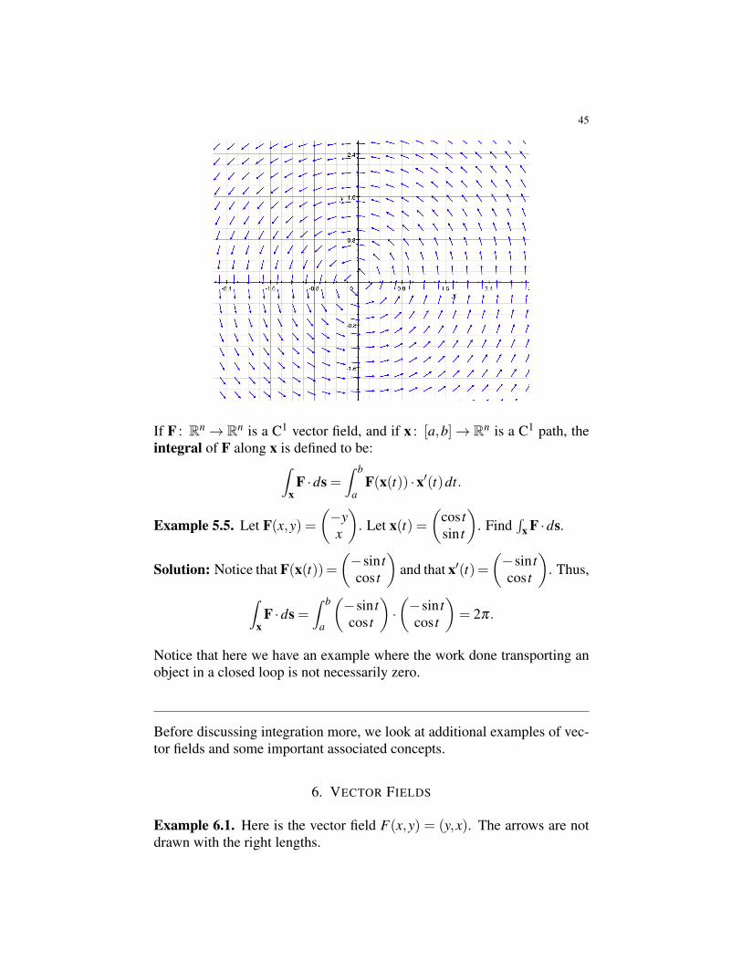
Example 5.4. Here is a picture of the vector field F(x,y) = (−y,x). Thearrows are not drawn with the correct lengths.
45
If F : Rn→ Rn is a C1 vector field, and if x : [a,b]→ Rn is a C1 path, theintegral of F along x is defined to be:∫
xF ·ds =
∫ b
aF(x(t)) ·x′(t)dt.
Example 5.5. Let F(x,y) =(−yx
). Let x(t) =
(cos tsin t
). Find
∫x F ·ds.
Solution: Notice that F(x(t))=(−sin tcos t
)and that x′(t)=
(−sin tcos t
). Thus,
∫x
F ·ds =∫ b
a
(−sin tcos t
)·(−sin tcos t
)= 2π.
Notice that here we have an example where the work done transporting anobject in a closed loop is not necessarily zero.
Before discussing integration more, we look at additional examples of vec-tor fields and some important associated concepts.
6. VECTOR FIELDS
Example 6.1. Here is the vector field F(x,y) = (y,x). The arrows are notdrawn with the right lengths.
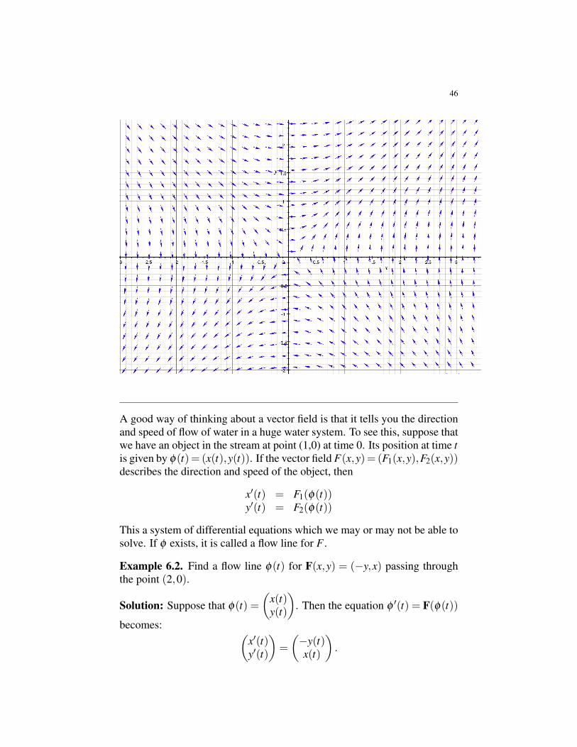
46
A good way of thinking about a vector field is that it tells you the directionand speed of flow of water in a huge water system. To see this, suppose thatwe have an object in the stream at point (1,0) at time 0. Its position at time tis given by φ(t)= (x(t),y(t)). If the vector field F(x,y)= (F1(x,y),F2(x,y))describes the direction and speed of the object, then
x′(t) = F1(φ(t))y′(t) = F2(φ(t))
This a system of differential equations which we may or may not be able tosolve. If φ exists, it is called a flow line for F .
Example 6.2. Find a flow line φ(t) for F(x,y) = (−y,x) passing throughthe point (2,0).
Solution: Suppose that φ(t) =(
x(t)y(t)
). Then the equation φ ′(t) = F(φ(t))
becomes: (x′(t)y′(t)
)=
(−y(t)x(t)
).

47
Thus we are looking for function x and y so that
x′(t) = −y(t)y′(t) = x(t)x(0) = 2y(0) = 0
The differential equations make us remember that sin and cos have deriva-tives related to each other in the way that we need.
Thus,
φ(t) =(
2cos t2sin t
)is the flow line we are looking for.
Example 6.3. Let F(x,y)= (y,x). Find flow lines through (1,1) and through(1,0).
Answer: Let φ(t) =(
x(t)y(t)
)be a flow line. Then,
x′(t) = y(t)y′(t) = x(t)
As a first guess, we try x(t) = et and y(t) = et . Sure enough, φ(t) =(
et
et
)is a flow line for F passing through (1,1).
To find a flow line passing through (1,0) more ingenuity is required. Even-tually, we might come up with:
φ(t) =(
cosh tsinh t
)=
((et + e−t)/2(et− e−t)/2
)
The image of this second flow line in the vector field F is pictured below.
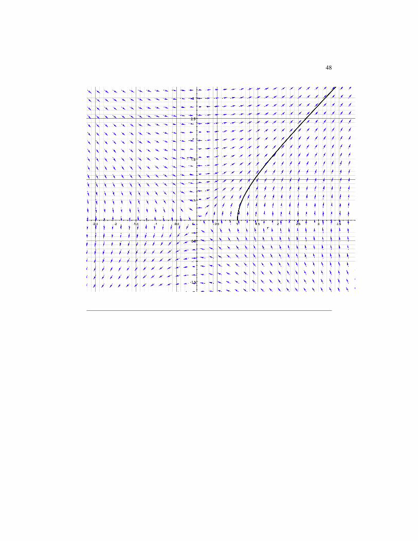
48

49
6.1. Gradient. Define the gradient by ∇ : C1(Rn)→ Rn by
grad f = ∇ f = (∂
∂x1,
∂
∂x2, . . . ,
∂
∂xn).
If we think of f ∈C1(Rn) as a scalar field, then ∇ (the gradient) converts thescalar field into a vector field. The vectors point in the direction of greatestincrease of f .
Example 6.4. Consider f : R2→ R defined by f (x,y) = sinxcosy. Then∇ f = (cosxcosy,−sinxsiny). Below is the vector field ∇ f on top of thescalar field f . Contour lines have been drawn on the scalar field so that youcan see how the vectors ∇ f are perpendicular to the contour lines.
If f : Rn→ R is a scalar field and if F = ∇ f , we say that f is a potentialfunction for F and that F is a gradient field or a conservative vector field.
For a fixed constant c, the set of points {x : f (x) = c} is called an equipo-tential set for f or F.
Example 6.5. Find a potential function for F(x,y) =(−xy
).
Answer: The function f (x,y) = −12x2 + 1
2y2 is a potential function for Fsince ∇ f = F. The hyperbolae
−12
x2 +12
y2 = c

50
are the equipotential lines for f . Notice in the figure below, that the equipo-tential line is perpendicular to a flow line. The flow line is black and theequipotential line is red.
Theorem 6.6. Suppose that F is a conservative vector field with potentialfunction f . Suppose that L is a smooth equipotential line for f and that φ isa flow line for F intersecting L. Then L and φ are perpendicular.
Proof. Suppose that φ and L intersect at a point x0 and that L has a unittangent vector v at x0. Since f is constant along L, the directional derivative∂
∂v f (x0) is equal to zero. By a standard result from Calculus II, ∂
∂v f (x0) =∇ f (x0) · v. Since this is zero, ∇ f (x0) = F(x0) is perpendicular to L atx0. �
Another very useful fact is:
Theorem 6.7. Suppose that F is a gradient field and that φ is a flow linewith ||φ ′(t)||> 0 for all t. Then φ does not close up on itself; in fact, for allt1 and t2 with t1 6= t2, φ(t1) 6= φ(t2).
Proof. Since F is a gradient field, there exists a potential function f for F.Consider g(t) = f (φ(t)). Then
g′(t) = D f (φ(t))φ ′(t) = ∇ f (φ(t)) ·φ ′(t)
Since F = ∇ f and since φ ′(t) = F(φ(t)), we have
g′(t) = F(φ(t)) ·F(φ(t)) = ||F(φ(t))||2 = ||φ ′(t)||2 > 0.
Thus, g′(t)> 0 for all t. In particular, g(t) = f (φ(t)) is a strictly increasingfunction.
51
Suppose that there exist t1 6= t2 such that φ(t1) = φ(t2). Then g(t1) = g(t2),but this contradicts the fact that g is strictly increasing. Hence, φ(t1) 6= φ(t2)for all t1 6= t2. �
Example 6.8. The vector field F(x,y) = (−y,x) has φ(t) = (cos t,sin t) asa flow line. Since φ(0) = φ(2π), the vector field F is not a gradient field.
The most important theorem of this subsection is a version of the Funda-mental Theorem of Calculus for conservative vector fields:
Theorem 6.9. Suppose that F = ∇ f is a C1 conservative vector field on Rn.Let x : [a,b]→ Rn be a path, then∫
xF ·ds = f (x(b))− f (x(a)).
Notice that one implication of this theorem is that the path integral of aconservative vector fields depends only on the potential function and theendpoints of the path, but not on the path itself. This suggests the followingdefinition (which applies to any vector field, not just conservative ones.)
Definition 6.10. A vector field F defined on a region D ⊂ Rn has pathindependent line integrals if whenever x : [a,b]→ D and y : [c,d]→ Dare paths such that x(a) = y(c) and x(b) = y(d) we have∫
xF ·ds =
∫y
F ·ds.
In other words, line integrals depend only on the endpoints and direction ofthe path.
Theorem 6.9 has the immediate consequence:
Corollary 6.11. Conservative vector fields have path independent line inte-grals.
We now prove Theorem 6.9.
proof of Theorem 6.9. Recall that F = ∇ f . By the chain rule:ddt
f (x(t)) = ∇ f (x(t)) ·x′(t) = F(x(t)) ·x′(t).
Hence, ∫ b
a
ddt
f (x(t))dt =∫ b
aF(x(t)) ·x′(t)dt.

52
We can evaluate the left hand side using the Fundamental Theorem of Cal-culus (version 2) to conclude that
f (x(b))− f (x(a)) =∫ b
aF(x(t)) ·x′(t)dt.
The right hand side is just one piece of the definition of line integral and sowe have:
f (x(b))− f (x(a)) =∫
xF ·ds
as desired. �
By using the Fundamental Theorem of Calculus (version 1) we can actuallyalso prove the converse to Theorem 6.9.
Theorem 6.12. Suppose that F is a C1 vector field defined on an open re-gion D in Rn. If F has path independent line integrals then F is conservative.
Proof. The only way we have of showing a vector field is conservative isto construct a potential function, so that is what we do. For simplicity, weassume that D has the property that for any two points a and b in D, thereis a C1 path joining them.
We need to define a C2 potential function f : D→ R2 for F. To that end,let a ∈ D, be considered as a basepoint. If x ∈ D, choose a path φ joining ato x and define f (x) =
∫φ
F ·ds. Notice that definition of f requires that thepath φ be chosen, but that the choice does not matter – any two paths willgive the same answer, by our hypothesis.
We need to show that f is differentiable and that ∇ f = F. We do this byexamining the directional derivatives of f .
Let u be a unit vector. Since D is open, there exists an open disc centered atx and contained in D. Choose h ∈ R small enough so that the vector x+huis in this disc. Let φ be a path from a to x and let ψ be a straight line pathin D from x to x+h. Then:
1h( f (x+h)− f (x) =
1h
(∫φ
F ·ds+∫
ψF ·ds−
∫φ
F ·ds)
=1h∫
ψF ·ds
Since ψ is a straight line path, we may assume that ψ(t) = x+ tu for 0 ≤t ≤ h. Then ψ ′(t) = u. The directional derivative of f in the direction u isthen:

53
limh→01h f (x+hu)− f (x) =limh→0
1h∫
ψF ·ds =
limh→01h∫ h
0 F(ψ(t)) ·u)dt =
When h is very small, F(ψ(t)) ≈ F(x) with the approximation improvingas h→ 0. Thus, if u is constant, we have the directional derivative of f inthe u direction as:
limh→01h( f (x+h)− f (x)) =
limh→01h∫ h
0 F(ψ(t)) ·u)dt =
limh→01h∫ h
0 F(x) ·udt =limh→0
1h(F(x) ·u)h =
F(x) ·u.
By making wise choices of h, we see that ∂ f∂x = F · i and ∂ f
∂y = F · j. Conse-quently, ∇ f = F. Furthermore, because F is C1, f is differentiable and isC2. �

54
6.2. Curl. If C is a closed curve, the circulation of a vector field F aroundC is defined to be
∫C F · ds. In the previous section, among other things,
we say that the circulation around any closed curve of a conservative vectorfield is 0. In the homework, you will show that Theorem 6.12 is in factequivalent to the statement that if a vector field has the property that forall closed curves C the circulation around C is 0 then F is conservative.Does this mean that a non-conservative vector field always has some kindof swirling or rotation? In this section we make the concept precise and willbegin exploring the nuances of the answer. We begin with an example.
Example 6.13. Let F(x,y) =(
0x
). It is shown below:
-4.8 -4 -3.2 -2.4 -1.6 -0.8 0 0.8 1.6 2.4 3.2 4 4.8
-3.2
-2.4
-1.6
-0.8
0.8
1.6
2.4
3.2
Notice that the arrows get longer and longer as we move out the x axis.Consider circles Cr of radius r centered at the origin. The circulation of Faround Cr is simply the line integral
∫Cr
F ·ds. We can easily calculate thisby parameterizing Cr as:
Cr(t) = r(
cos tsin t
)for 0≤ t ≤ 2π.
We have:
C′r(t) = r(−sin tcos t
).

55
Thus, ∫Cr
F ·ds =∫ 2π
0
(0
r cos t
)·(−r sin tr cos t
)dt
=∫ 2π
0 r2 cos2 t dt=
∫ 2π
0 r2(cos2t +1)/2= πr2
Since this integral is non-zero (for r > 0), the field is not conservative. Fur-thermore, there is clearly some sort of rotation about the origin even thoughall flow lines are straight lines. Even on small scales this rotation persistsas we can see by taking the limit of the circulation around Cr divided by thearea enclosed by Cr:
limr→0+
1πr2
∫Cr
F ·ds = limr→0+
(1
πr2 )(πr2) = 1.
This is an example of what is called the “scalar curl” of a 2-dimensionalvector field.
Definition 6.14. Suppose that F is a C1 vector field defined on an openregion D⊂R2. Let a ∈D. For each r, let Cr be a circle of radius r centeredat a and oriented counter-clockwise. Choose r small enough so that the discDr bounded by Cr is contained in D. Then, the scalar curl of F at a isdefined to be:
scalarcurlF(a) = limr→0+
1Area(Dr)
∫Cr
F ·ds.
Since the integral of a conservative vector field around a closed curve is 0,we see immediately that the scalar curl of a conservative vector field at anypoint a is zero.
How important is it that the curves Cr be circles? Not that important, as thenext example suggests.
Example 6.15. Let F(x,y) =(
0x
). Let Cr be the square with corners at
(−r,−r), (r,−r), (r,r), and (−r,r) oriented counter-clockwise. Let Dr bethe solid square bounded by Cr. We will compute
limr→0+
1Area(Dr)
∫Cr
F ·ds.

56
To do that we need to parameterize Cr. Cr consists of four line segmentswhich we may paramterize as:
L1(t) = (t,−r) −r ≤ t ≤ rL2(t) = (r, t) −r ≤ t ≤ rL3(t) = (−t,r) −r ≤ t ≤ rL4(t) = (−r,−t) −r ≤ t ≤ r.
Notice that:L1(t) = (1,0) −r ≤ t ≤ rL2(t) = (0,1) −r ≤ t ≤ rL3(t) = (−1,0) −r ≤ t ≤ rL4(t) = (0,−1) −r ≤ t ≤ r.
We have that∫Cr
F ·ds =∫
L1F ·ds+
∫L2
F ·ds+∫
L3F ·ds+
∫L4
F ·ds
=∫ r−r
(0t
)·(
10
)+
(0r
)·(
01
)+
(0−t
)·(−10
)+
(0−r
)·(
0−1
)= 0+ r(2r)+0+ r(2r)= 4r2.
The area Dr is (2r)2 = 4r2. So
limr→0+
1Area(Dr)
∫Cr
F ·ds = limr→0+
14r2 (4r2) = 1.
This is the same answer as in the previous example.
Example 6.16. Compute the scalar curl of F(x,y) = (−y,x) at each a in R2.
Let Cr be the circle of radius r centered at a = (a1,a2). The curve Cr can beparameterized as:
Cr(t) =(
a1 + r cos ta2 + r sin t
)for 0≤ t ≤ 2π.
We have
C′r(t) =(−r sin tr cos t
).
Thus, the circulation of F around Cr is:∫Cr
F ·ds =∫ 2π
0
(−a2− r sin ta1 + r cos t
)·(−r sin tr cos t
)=
∫ 2π
0 −(a2 + r sin t)(−r sin t)+(a1 + r cos t)(r cos t)=
∫ 2π
0 ra2 sin t + ra1 cos t + r2
= 2πr2.

57
Hence, the scalar curl of F at a is:
limr→0+
1πr2
∫Cr
F ·ds = limr→0+
1πr2 (2πr2) = 2.
Can we define some sort of “curl” for vector fields in R3? We sure can:
Definition 6.17. Suppose that F is a C1 vector field defined on an opensubset of R3. Let a be a point in the domain of F. Let Cr be a circle in thexy-plane centered at a of radius r and with the right-hand orientation aroundthe positive z-axis. Let Dr be a circle in the yz-plane centered at a of radiusr and with the right-hand orientation around the positive x-axis. Let Er bea circle in the xz-plane centered at a of radius r and with the right-handorientation around the positive y-axis. Choose r > 0 small enough so thateach of these circles is contained in the domain of F. Then the curl of Fand a is defined to be:
curlF(a) = limr→0+
1πr2
∫DrF ·ds∫
ErF ·ds∫
CrF ·ds
.
The circles Cr, Dr and Er are pictured below (with a = 0.
Notice that if F =
F1F20
, is actually 2-dimensional, then the k component
of curlF(a) is the scalar curl of F.
Notice that, based on this definition, it is fair to say that curl measures the“infinitesimal rotation” of a vector field F about a point a. Informally, ifcurlF(a) 6= 0, then a paddle-wheel dropped in the vector field at F will spinaround an axis pointing in the direction of curlF(a).

58
Although the definition of curl tells us what it is, it doesn’t provide a goodmeans of calculating it. After we learn Stokes’ theorem, we’ll be able toprove the following:
Theorem 6.18. Suppose that F =
MNP
. Then
curlF(a) = ∇×F(a)
= det
i j k∂
∂x∂
∂y∂
∂ zM N P
=
∂
∂yP(a)− ∂
∂ zN(a)∂
∂ zM(a)− ∂
∂xP(a)∂
∂xN(a)− ∂
∂yM(a)
.
Example 6.19. Calculate the curl of F(x,y) = (−y,x).
Solution:
curlF(x,y) = det
i j k∂
∂x∂
∂y∂
∂ z−y x 0
=
∂
∂y0− ∂
∂ z(x)∂
∂ z(−y)− ∂
∂x(0)∂
∂x(x)−∂
∂y(−y)
=
002
.
59
6.3. Divergence. In the last section we saw two formulations of curl – onein terms of integrals and one in terms of partial derivatives. The formula interms of integrals told us what curl means but the formula with derivativestells us how to calculate it. In this section we’ll do something similar forthe “divergence” of a vector field. At present, we can only do this in 2-dimensions. After we introduce the notion of surface integral, we’ll also beable to define divergence in 3-dimensions.
Before defining divergence, we need to define the concept of “outwardpointing normal” to a curve.
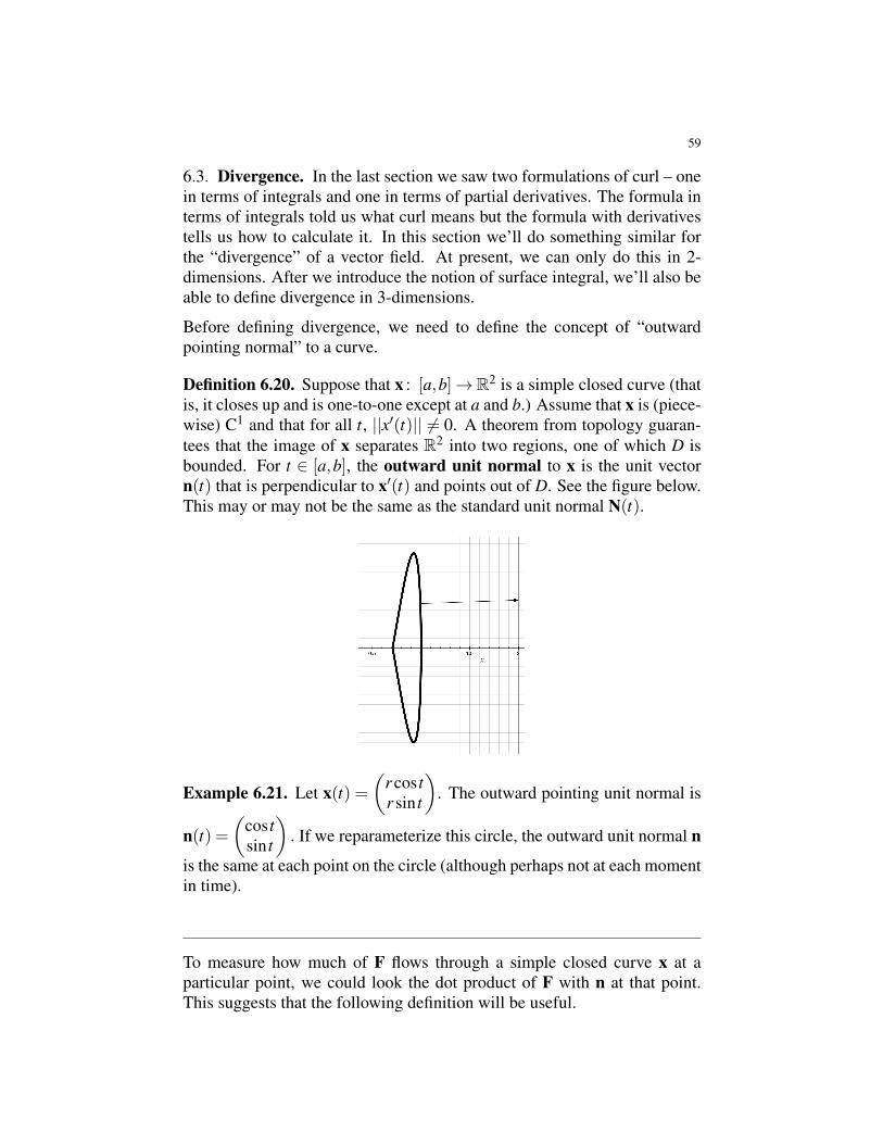
Definition 6.20. Suppose that x : [a,b]→ R2 is a simple closed curve (thatis, it closes up and is one-to-one except at a and b.) Assume that x is (piece-wise) C1 and that for all t, ||x′(t)|| 6= 0. A theorem from topology guaran-tees that the image of x separates R2 into two regions, one of which D isbounded. For t ∈ [a,b], the outward unit normal to x is the unit vectorn(t) that is perpendicular to x′(t) and points out of D. See the figure below.This may or may not be the same as the standard unit normal N(t).
Example 6.21. Let x(t) =(
r cos tr sin t
). The outward pointing unit normal is
n(t) =(
cos tsin t
). If we reparameterize this circle, the outward unit normal n
is the same at each point on the circle (although perhaps not at each momentin time).
To measure how much of F flows through a simple closed curve x at aparticular point, we could look the dot product of F with n at that point.This suggests that the following definition will be useful.

60
Definition 6.22. Let C be a simple closed (piecewise) C1 curve in R2 pa-rameterized by x : [a,b]→R2. Let n(t) be the outward unit normal of x(t).If F is a C1 vector field defined on an open set containing C, the flux of Fthrough C is defined to be ∫
CF ·nds
Notice that this is a line integral of a scalar field.
Example 6.23. Let F(x,y) =(
xy
)and let Cr be a circle of radius r centered
at the origin. Then the flux of F through Cr is:∫Cr
F ·nds.
To calculate this, parameterize Cr as x(t) = r(cos t,sin t) for 0 ≤ t ≤ 2π sothat n(t) = (cos t,sin t). Recall that ||x′(t)||= r.Then:∫
Cr
F ·nds =∫ 2π
0
(r cos tr sin t
)·(
cos tsin t
)rdt = 2πr2.
Example 6.24. Let F(x,y) = (−y,x) and let Cr be the circle of radius rcentered at the origin. Then the flux of F through Cr is 0.
If we want to measure how much a vector field F is spreading out from apoint a or sucked into a point a, we take the limit as r→ 0+ of the fluxthrough a circle of radius r centered at a divided by the area enclosed by thecircle.
Definition 6.25. Suppose that F is a C1 vector field defined on an opensubset of R2. If a is a point in the domain of F, then the divergence of F ata is defined to be:
divF(vecta) = limr→0+
1πr2
∫Cr
F ·nds.
where Cr is a circle in the domain of F centered at a of radius r and n is itsoutward pointing unit normal.
Example 6.26. Based on our previous calculations we can deduce that thedivergence of the vector field (x,y) at 0 is 2 and the divergence of (−y,x) at0 is 0.
We will be able to prove the next theorem after we discuss the planar diver-gence theorem:

61
Theorem 6.27. Suppose that F(x,y) =(
M(x,y)N(x,y)
)is a C1 vector field de-
fined on an open subset of R2. Then
divF(x,y) =∂
∂xM(x,y)+
∂
∂yN(x,y).
In fact, in all dimensions we could (and do) define the divergence of a vectorfield F = (F1, . . . ,Fn) to be
divF(x) =n
∑i=1
∂
∂xiFi(x).
In the previous section we showed that the curl of a gradient field is 0. Nowwe show that the divergence of curl is 0.
Theorem 6.28. Suppose that G is a C2 vector field defined on an opensubset of R2 or R3. Then divcurlG = 0.
Theorem 6.29. This is an exercise that uses Theorem 6.27 and Theorem6.18.
6.4. From Vector Calculus to Cohomology. Gradient is an operator thatconverts a scalar field into a vector field. Curl converts a vector field intoanother vector field. Divergence converts a vector field into a scalar field.Furthermore, (assuming all scalar fields and vector fields in question areC2) we have that curlgrad = 0 and divcurl = 0. These observations are thebasis for something called “cohomology theory”. More will be said at theend of these notes.

62
7. REVIEW: DOUBLE INTEGRALS
7.1. Integrating over rectangles. Suppose that R = [a,b]× [c,d] is a rec-tangle in the xy-plane with corners at the points (a,c), (a,d), (b,c) and(b,d). Let f : R→ R is a scalar field. Here is a picture of the situation:
we define the double integral∫∫R
f dA as follows.
Subdivide R into n rectangles R1, . . . ,Rn (each with sides parallel to theaxes). Let ∆Ai denote the area of rectangle i. Choose a point ci in rectangleRi. Define the nth Riemann sum to be
Sn =n
∑i=1
f (ci)∆Ai
Notice that Sn is an approximation to the (signed) volume between the graphof f in R3 and the rectangle R in the xy-plane. Here is another interpretationof Sn: If all the rectangles are chosen to have the same area ∆Ai = ∆A,then ∆A = Area(R)/n. The average value of f on the rectangle can beapproximated by:
1n ∑
ni=1 f (ci) =
∆AArea(R) ∑
ni=1 f (ci) =
1Area(R) ∑
ni=1 f (ci)∆A =
1Area(R)Sn
63
We then define ∫∫R
f dA = limmax∆Ai→0
Sn
This integral represents the volume between the graph of f in R3 and therectangle R⊂ R2.
The average value of f could be defined to be1
Area(R)
∫∫R
f dA.
Fubini’s theorem is what we usually use to calculate double integrals. Inmany situations, Fubini’s theorem tells us that a double integral can berewritten as an iterated integral, that is as two Calc I integrals.
Theorem 7.1 (Fubini’s theorem). Suppose that R = [a,b]× [c,d] is a rec-tangle in R2 and that f : R→R is a bounded function such that the discon-tinuities of f have zero area and every line parallel ot the coordinate axesmeets the set of discontinuities in finitely many points. Then∫∫
R
f dA =∫ b
a
∫ d
cf (x,y)dydx =
∫ d
c
∫ b
af (x,y)dxdy.
Example 7.2. Let R = [0,2π]× [0,π] and let f (x,y) = sinxcosy. Find∫∫R
f dA.
Solution: By Fubini’s theorem:∫∫R
f dA. =∫ 2π
0∫
π
0 sinxcosydydx
=∫ 2π
0 sinxsiny∣∣∣π0
dx
=∫ 2π
0 0dx= 0.
7.2. Integrating over non-rectangular regions. There are two ways ofdefining an integral of a scalar field over a non-rectangular region. Bothreduce the problem to integrating over rectangles. The first will suggest agood way of doing calculations but the second produces an integral that isdefined in more situations. If both integrals exist, they give the same answer.
For our purposes, it will suffice to consider the situation when D ⊂ R2 is aclosed and bounded region and when f : D→ R is a continuous function.We seek to define
∫∫D
f dA.
64
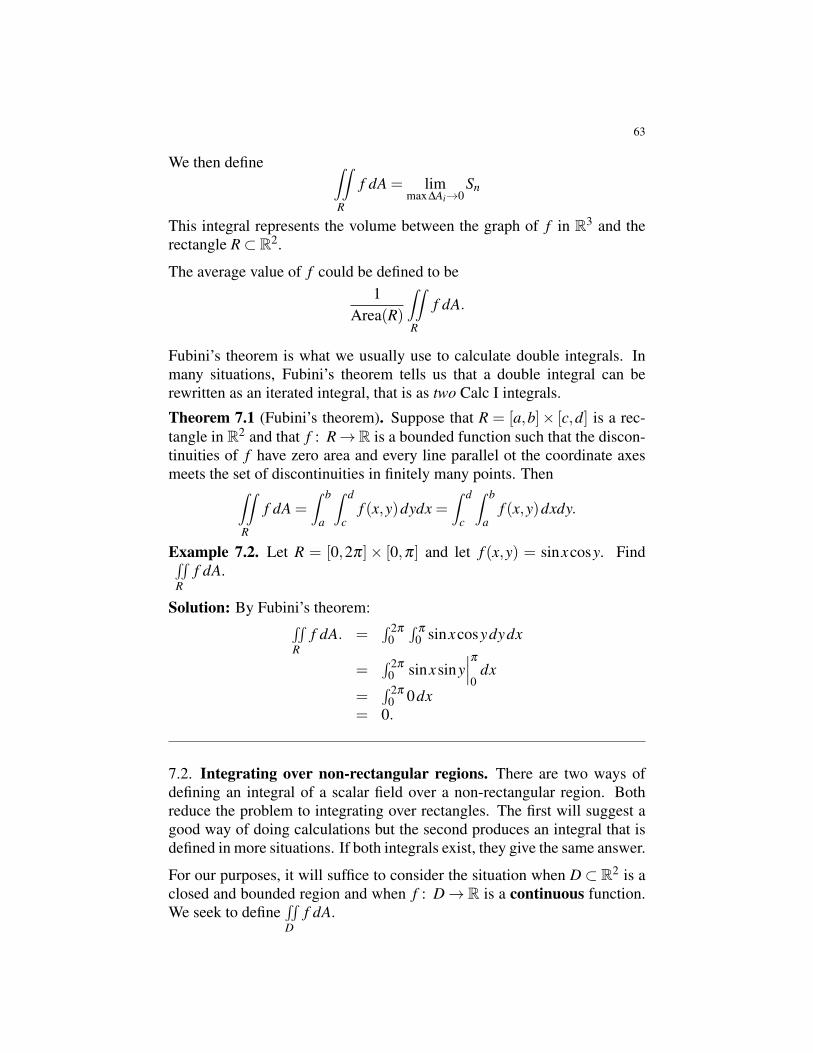
Here is a picture of a region D bounded by an ellipse and the scalar fieldf (x,y) = sinxcosy.
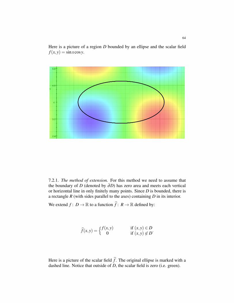
7.2.1. The method of extension. For this method we need to assume thatthe boundary of D (denoted by ∂D) has zero area and meets each verticalor horizontal line in only finitely many points. Since D is bounded, there isa rectangle R (with sides parallel to the axes) containing D in its interior.
We extend f : D→ R to a function f : R→ R defined by:
f (x,y) ={ f (x,y) if (x,y) ∈ D
0 if (x,y) 6∈ D.
Here is a picture of the scalar field f . The original ellipse is marked with adashed line. Notice that outside of D, the scalar field is zero (i.e. green).

65
We now define: ∫∫D
f dA =∫∫R
f dA.
7.2.2. The method of exhaustion. For this method, we assume that D is anopen set in R2. Subdivide the region D into m rectangles R1, . . . ,Rm so thatD⊂
⋃mi=1Ci. (That is the rectangles cover D.) Let ∆A be the maximum area
of any rectangle. Choose the numbering so that rectangles R1, . . . ,Rn arecompletely contained inside D. Define:∫∫
D
f dA = lim∆A→0
n
∑i=1
∫∫Ri
f dA.
This integral is called the improper integral of f on D.
If D is a closed, bounded region in R2, we now have two possible definitionsof∫∫D
f dA. We could try to define it using the method of extension or define
it using the method of exhaustion on the interior of the region. The improperintegral will always exist, although the usual integral (defined using themethod of extension) may not exist. If both exist, however, they are equal.See Theorem 15.4 of Munkres’ Analysis on Manifolds.
7.2.3. Calculating integrals over non-rectangular regions. The advantageof the definition of the integral
∫∫D
f dA using the method of extension is that
we can apply Fubini’s theorem to the integral∫∫R
f dA. Doing so provides

66
the following methods of converting a double integral∫∫D
f dA over a non-
rectangular region D into an iterated integral. To describe the method wefirst introduce some terminology.
Suppose that D⊂R2 is a closed, bounded region. We say that it is verticallyconvex (or Type I) if every vertical line segment having endpoints in Ditself lies entirely in D.
Example 7.3. Here is an example of a vertically convex region:
Example 7.4. The region bounded by the black curve is not vertically con-vex, since there exists a vertical line segment (in red) having both endpointsinside the region but not lying entirely in the region itself.

67
We say a closed, bounded region D ⊂ R2 is horizontally convex (or TypeII) if every horizontal line segment with both endpoints in the region itselflies completely in the region.
Example 7.5. Here is an example of a horizontally convex region.
68
Finally, we say that a region is Type III if it is both of Type I and Type II.Regions bounded by circles and squares are examples of Type III regions.
Notice that if a region D is vertically convex, then it can be described as:
D ={(x,y) ∈ R2 : a≤ x≤ b
γ(x)≤ y≤ δ (x)
}where γ and δ are functions of x.
Example 7.6. The region from Example 7.3 can be described as:
D ={(x,y) ∈ R2 :
−3≤ x≤ 3−√
1− x2/9≤ y≤ sin(2(x+3))+2
}
Notice that if a region D is horizontally convex, then it can be described as:
D ={(x,y) ∈ R2 : c≤ y≤ d
α(y)≤ x≤ α(y)
}where α and β are functions of y.
Example 7.7. The region from Example ?? can be described as:
D ={(x,y) ∈ R2 :
−2≤ y≤ 2√1− y2/4−2≤ x≤ sin(4y)+2
}
Now here’s how to integrate a scalar field f over a non-rectangular regionD assuming that the integral defined by extension exists.
• If D is vertically convex, write:
D ={(x,y) ∈ R2 : a≤ x≤ b
γ(x)≤ y≤ δ (x)
}Then ∫∫
D
f dA =∫ b
a
∫δ (x)
γ(x)f (x,y)dydx.
• If D is horizontally convex, write:
D ={(x,y) ∈ R2 : c≤ y≤ d
α(y)≤ x≤ α(y)
}Then ∫∫
D
f dA =∫ d
c
∫β (y)
α(y)f (x,y)dxdy.

69
Example 7.8. Let D be the region from Example 7.3. Let f (x,y) = xy2.Then: ∫∫
D
f dA =∫ 3
−3
∫ sin(2(x+3)+2
−√
1−x2/9xy2 dydx.
These integrals can easily be plugged into Mathematica or similar program.
Example 7.9. Let D be the region from Example ??. Let f (x,y) = cos(xy).Then: ∫∫
D
f dA =∫ 2
−2
∫ sin(4y)+2√
1−y2/4−2cos(xy)dA.
Example 7.10. Let D be the region between the graphs of y = (x−1)2 andy =−(x−1)2 +2. Let f (x,y) = xy. Find
∫∫D
f dA.
Solution: Some easy algebra shows that the two curves intersect at thepoints (0,1) and (2,1). We are given the region as a Type I (verticallyconvex) region. So:∫∫
D
f dA =∫ 2
0
∫ −(x−1)2+2
(x−1)2xydydx.
Sometimes there are other tricks we can use to find integrals.
Example 7.11. Let D be the square region with vertices at (−1,0), (1,0),(0,1) and (0,−1). Let f (x,y) = x2 + y2. Find
∫∫D
f dA.
Solution: Notice that f (x,y) = r2 where r = ||(x,y)||. Thus, if the plane isrotated about the origin by any angle f (x,y) will remain unchanged. Rotate

70
the plane so that D is a square centered at the origin and with sides parallelto the x and y axes. Call this new square D′. Since the value of f doesn’tchange after the rotation, ∫∫
D
f dA =∫∫D′
f dA.
Both D and D′ have sides of length√
2 and so the corners of D′ are at(±√
2,±√
2) and (±√
2,∓√
2). Thus,∫∫D
f dA =∫∫D′
f dA =∫ √2
−√
2
∫ √2
−√
2x2 + y2 dxdy.
This last integral can be evaluated easily by hand:∫√2−√
2
∫√2−√
2x2 + y2 dxdy =
∫√2−√
223(2
3/2)+2√
2y2 dy
= 43(2
3/2)(21/2)+ 4√
23 (23/2)
= 323

71
8. INTERLUDE: THE FUNDAMENTAL THEOREM OF CALCULUS ANDGENERALIZATIONS
8.1. 0 and 1 dimensional integrals. Let I = [a,b] be an interval (orientedfrom a to b) If F : I→ R is a differentiable function, then you learn in onevariable calculus that ∫
I
ddt
F(t)dt = F(b)−F(a).
To generalize this theorem to higher dimensions we introduce some newterminology.
Terminology 1: If p ∈ R is a point, then say that p has “positive orien-tation” if we place an arrow on it pointing to the right. The point p has“negative orientation” if we put an arrow on it pointing to the left. If wehave chosen an orientation for p, we say that p is oriented. If A is a fi-nite subset of R and if each point in A has been given an orientation (notnecessarily the same), we say that A is oriented.
Terminology 2: Suppose that p∈R is an oriented point and that f : R→Ris a function. If p has positive orientation, define
∫p f = f (p). If p has
negative orientation, define∫
p f =− f (p). If A = {p1, . . . , pn} is a finite setof oriented points in R, define
∫A = ∑
ni=1∫
pif .
Terminology 3: Suppose that a < b are real numbers. The interval [a,b]is positively oriented and the interval [ba] is negatively oriented. (Thinkof an arrow running from the small number a to the big number b. If thearrow points right, the interval is positively oriented; if it points left it isnegatively oriented.) If I is an interval in R with endpoints a < b, then the“boundary” of I, denoted ∂ I, is the set {a,b}. If I has positive orientation,we assign the points of ∂ I the orientation with arrows pointing out of I. IfI has negative orientation, we assign the points of ∂ I, the orientations witharrows pointing into I. We say that ∂ I has the orientation “induced” by theorientation from I.
Suppose that I = [a,b] has positive orientation (i.e. a < b). Let J = [b,a]be the same interval but with the opposite orientation. If f : R → R isintegrable, then by definition∫
If =
∫ b
af (x)dx and
∫J
f =∫ a
bf (x)dx =−
∫I
f .
The fundamental theorem of calculus can then be stated as
72
Theorem 8.1 (Fundamental Theorem of Calculus). Suppose thatF : R→ R is a C1 function. Let DF : R→ R be its derivative. LetI ⊂ R be an oriented interval and give ∂ I the induced orientation.Then ∫
IDF =
∫∂ I
F.
Notice that the FTC says that the 1-dimensional integal of a derivative isequal to a certain 0-dimensional integral (over the boundary) of the anti-derivative.
8.2. Green’s theorem.
Theorem 8.2 (Green’s Theorem). Suppose that D⊂R2 is closed and boundedand that ∂D is (piecewise) C1. Orient ∂D so that D is always on the left. IfF : D→ R2 is a C1 scalar field then:∫∫
D
scalarcurl(F)dA =∫
∂D
F ·ds
Notice that this relates a 2-dimensional integral of a “derivative” to a 1-dimensional integral of an “anti-derivative”.
Example 8.3. Let Dr be the disc of radius r in R2 centered at the origin.
Let Cr = ∂Dr oriented counterclockwise. Let F(xy) =(−yx
). We calculate
both sides of the equality in Green’s theorem to verify that Green’s theoremis true in this case.
The scalar curl of F is:
scalarcurl(F(x,y)) =∂
∂x(x)− ∂
∂y(−y) = 2.
Thus, ∫∫D
scalarcurl(F(x,y)dA =∫∫D
2dA = 2Area(D) = 2πr2.
The curve Cr can be parameterized as Cr(t) =(
r cos tr sin t
)for t ∈ [0,2π]. It is
evident that C′r(t) =(−r sin tr cos t
). Thus,
∫Cr
F ·ds =∫ 2π
0F(Cr(t)) ·C′r(t)dt =
∫ 2π
0r2 dt = 2πr2
73
Notice that indeed: ∫∫D
scalarcurl(F)dA =∫
CrF ·ds
Rather than using an orientation of ∂D that points in the direction of travel,we can also rephrase Green’s theorem so as to use a normal orientation of∂D.
Definition 8.4. Suppose that D ⊂ R2 is a closed, bounded region with ∂Dpiecewise C1. At each C1 point of ∂D, let n be the unit normal vector point-ing out of D. If x(t) = (x(t),y(t)) is a parameterization of ∂D with D alwayson the left, then the outward unit normal is n(t) = 1
||x′(t)||(y′(t),−x′(t)).
Theorem 8.5 (Planar Divergence Theorem). Suppose that D ⊂ R2 is aclosed, bounded region with ∂D piecewise C1. Let n be the outward point-ing unit normal to ∂D. Then, if F is C1:∫∫
D
divFdA =∫
∂DF ·nds.
Notice that once again we have a 2-dimensional integral of a derivativeequal to a 1-dimensional integral of an “antiderivative”. (Obviously theterminology from Calc I doesn’t match up exactly.) The right hand side ofthe equality above is called the “flux” of F across ∂D.
8.3. Stokes’ Theorem. We don’t have all the terminology available to usyet, but here’s the statement of Stokes’ theorem so that you can compare itto the other cases.
Theorem 8.6 (Stokes’ Theorem). Suppose that S is a (piecewise) C1 ori-entable surface in R3 and that ∂S is also piecewise C1. Give S an orienta-tion and give ∂S the orientation induced from S. Let F be a C1 vector fielddefined on an open set containing S. Then:∫∫
ScurlF ·dS =∫∂S
F ·ds
Once again we have a 2–dimensional integral of a derivative equal to a 1–dimensional integral of the anti-derivative. This theorem will eventuallymotivate us to define the notion of “surface integral”. We will have to talkabout parameterizing surfaces and orientations of surfaces, as well.

74
8.4. The Divergence Theorem. Once again, we don’t have all the termi-nology available to us, but here is the statement of the Divergence Theorem(also known as Gauss’ theorem).
Theorem 8.7 (The Divergence Theorem). Suppose that D⊂R3 is a closed,bounded region with ∂D a piecewise C1 surface. Give ∂D the normal ori-entation pointing out of D. Then∫∫∫
D
divFdV =∫∫∂D
F ·dS.
The integral on the left is the triple integral you encountered in Calc II. Theintegral on the right is a surface integral, which we have still to define. Inany case, you can see that we have a 3-dimensional integral of a “derivative”equal to a 2–dimensional integral of the “anti-derivative”.
8.5. Generalized Stokes’ Theorem. The divergence theorem is as far aswe’ll be able to go in our class, but you may wonder about a version of FTCin dimensions greater than 3. There is such a thing, called “GeneralizedStokes’ Theorem” (or simply “Stokes’ Theorem”. Here, for the record isthe statement. We won’t define any of the unknown terms in this class.
Theorem 8.8 (Generalized Stokes’ Theorem). Suppose that M is an ori-ented, smooth n-dimensional manifold with smooth boundary ∂M havingthe induced orientation. (The boundary of M is an (n−1) manifold.) Sup-pose that ω is an (n−1) form on M having compact support then∫
M
dω =∫
∂M
ω.
At the very least you can see an n-dimensional integral on the left and an(n− 1)-dimensional integral on the right. The integrand on the left is aderivative of the integrand on the right. And that’s all we’ll say about that!
75
9. BASIC EXAMPLES OF GREEN’S THEOREM IN ACTION
Theorem 9.1 (Green’s Theorem). Suppose that D⊂R2 is closed and boundedand that ∂D is (piecewise) C1. Orient ∂D so that D is always on the left. IfF : D→ R2 is a C1 scalar field then:∫∫
D
scalarcurl(F)dA =∫
∂D
F ·ds
If we write F(x,y) = M(x,y)i + N(x,y)j, then the conclusion of Green’stheorem can be written as:∫
∂DM dx+N dy =
∫∫D
(∂N∂x− ∂M
∂y
)dA.
Before proving (part of) Green’s theorem, we’ll look at some examples.
Example 9.2. For this example, let D⊂R2be the solid square with corners(1,−1), (1,1), (−1,1), and (−1,−1). We will need a parameterization of∂D. Since ∂D is made up of 4 line segments, we can parameterize them asfollows. For each of them 0≤ t ≤ 1.
L1(t) = (1,2t−1)L2(t) = (1−2t,1)L3(t) = (−1,1−2t)L4(t) = (2t−1,−1)
We will also need the derivatives:
L′1(t) = (0,2)L′2(t) = (−2,0)L′3(t) = (0,−2)L′4(t) = (2,0)
Example 1a: Let F(x,y) = (−x,y).
Example 1a.i: Compute∫
∂D F ·ds.
Answer: We have:∫∂D F ·ds =
∫ 10 F(L1(t)) ·L′1(t)dt +
∫ 10 F(L2(t)) ·L′2(t)dt+∫ 1
0 F(L3(t)) ·L′3(t)dt +∫ 1
0 F(L4(t)) ·L′4(t)dt
=∫ 1
0
(−1
2t−1
)·(
02
)+
(2t−1
1
)·(−20
)+
(1
1−2t
)·(
0−2
)+
(1−2t−1
)·(
20
)dt
=∫ 1
0 2(2t−1)+(−2)(2t−1)+(−2)(1−2t)+2(1−2t)dt= 0
76
Example 1a.ii: Compute∫∫D(curlF) ·kdA.
Answer: We have
curlF ·k =∂ (y)∂x− ∂ (−x)
∂y= 0.
Thus,∫∫D
curlF · kdA =∫∫D
0dA = 0. Notice that this matches the answer
from Example 1a.i, as predicted by Green’s theorem.
Example 1b: Let F(x,y) = (−y,x).
Example 1b.i Compute∫
∂D F ·ds.
Answer: We have:∫∂D F ·ds =
∫ 10 F(L1(t)) ·L′1(t)dt +
∫ 10 F(L2(t)) ·L′2(t)dt+∫ 1
0 F(L3(t)) ·L′3(t)dt +∫ 1
0 F(L4(t)) ·L′4(t)dt
=∫ 1
0
(1−2t
1
)·(
02
)+
(−1
1−2t
)·(−20
)+
(2t−1−1
)·(
0−2
)+
(1
2t−1
)·(
20
)dt
=∫ 1
0 2+2+2+2dt= 8
Example 1b.ii Compute∫∫D(curlF) ·kdA.
In this case, curlF ·k = 2. Thus,∫∫D
curlF ·kdA =∫ 1
−1
∫ 1
−12dA = 8.
Notice that this is the same as in Example 1b.i as predicted by Green’stheorem.
Example 9.3. Let F(x,y) = (sinx, ln(1+ y2)). Let C be a simple closedcurve which is made up of 24 line segments in a star shape. Compute∫
C Fds.
Answer: Let D be the region bounded by C. Notice that curlF = 0, so∫∫D
curlF · kdA = 0. By Green’s theorem, this is also the answer to the
requested integral.
Example 9.4. Let φ(t) =(
cos t sin(3t)sin t cos(3t)
)for 0≤ t ≤ π/2. Find the area of
the region D enclosed by φ .
77
Answer: Notice that φ travels clock-wise around D, we need it to gocounter-clockwise to use Green’s theorem. Changing the direction that φ
travels, changes the sign of a path integral of a vector field. Thus, by Green’stheorem, the area of D is given by∫∫
D1dA =−
∫φ
F ·ds,
where F is a vector field having the property that curlF = (0,0,1). Thevector field: F(x,y) = 1
2(−y,x) has that property. Thus,∫∫D 1dA = −
∫φ
F ·ds= −(1/2)
∫ π/20 (−sin t cos3t,cos t sin3t) ·φ ′(t)dt
= −(1/2)∫ π/2
0 cos3t sin3t−3sin t cos t dt= −(1/2)
∫ π/20 sin(6t)/2−3sin(2t)/2dt
= −(1/2)(1/6−3/2)= 2/3.
78
10. THE PROOF OF GREEN’S THEOREM
The proof of Green’s theorem relies heavily on the following fact:
Lemma 10.1. Suppose that R1 and R2 are two regions in R2 each withpiecewise C1 boundary and suppose that R1 and R2 intersect only along apath φ in their boundaries. Give ∂R1 the orientation with R1 on the leftand give ∂R2 the orientation with R2 on the left. Let R = R1∪R2 and give∂R the orientation having R on the left. Suppose that F is a C1 vector fielddefined on R. Then:∫
∂RF ·ds =
∫∂R1
F ·ds+∫
∂R2
F ·ds.
Proof. Since φ = R1∩R2, the orientations on ∂R1 and ∂R2 induce oppositeorientations on φ . We have proved that if x and y are orientation reversingreparameterizations of each other then∫
yF ·ds =−
∫x
F ·ds.
Let x be the parameterization of φ coming from a parameterization of ∂R1and let y be the parameterization of φ coming from a parameterization of∂R2.
Let ψ1 = ∂R1−φ and let ψ2 = ∂R2−φ . Then:∫∂R1
F ·ds =∫
ψ1
F ·ds+∫
xF ·ds
and
∫∂R2
F ·ds =∫
ψ2
F ·ds+∫
yF ·ds
Thus,∫∂R1
F ·ds+∫
∂R2
F ·ds =∫
ψ1
F ·ds+∫
xF ·ds+
∫ψ2
F ·ds+∫
yF ·ds
Since x and y are orientation-reversing reparameterizations of each other,we have ∫
∂R1
F ·ds+∫
∂R2
F ·ds =∫
ψ1
F ·ds+∫
ψ2
F ·ds
But this is exactly∫
∂R F ·ds. �
79
Sketch of Proof of Green’s Theorem. Let D be a region in R2 satisfying thehypotheses of Green’s theorem. Recall that for a point a ∈ D we have:
scalarcurl(F)(a) = limArea(E)→0+
1Area(E)
∫∂E
F ·ds.
where E is any region enclosing a.
From topology, we know that for any ε > 0, and for large enough n, theregion D can be subdivided into n triangles having piecewise C1 boundaryand each having area less than ε . Let T1, . . . ,Tn be those triangles. Orient theboundaries of each of those triangles so that the triangle is on the left. Byrepeatedly applying the previous lemma and using the additivity propertiesof the double integral we have:∫
∂D
F ·ds =n
∑i=1
∫∂Ti
F ·ds.
Taking the limit we obtain:∫∂D
F ·ds = limε→0+
n
∑i=1
∫∂Ti
F ·ds.
In each triangle Ti, choose a point ci. By the definition of scalar curl, if ε issmall enough,
Area(Ti)scalarcurlF(ci)≈∫
∂Ti
F ·ds.
Thus, for ε small enough,n
∑i=1
Area(Ti)scalarcurlF(ci)≈n
∑i=1
∫∂Ti
F ·ds.
When we take the limit as ε → 0+, we get equality:
limε→0+
n
∑i=1
Area(Ti)scalarcurlF(ci) = limε→0+
n
∑i=1
∫∂Ti
F ·ds.
The left hand side is simply the limit of Riemann sums (using trianglesinstead of squares) and the right hand side we have already calculated. So:∫∫
D
scalarcurlFdA =∫
∂D
F ·ds.
�

80
11. APPLICATIONS OF GREEN’S THEOREM
11.1. Finding Areas. Green’s theorem says that (under certain hypothe-ses) ∫∫
D
scalar curlFdA =∫
∂D
F ·ds
We recall that the area of a region D is equal to∫∫D
1dA. Thus, if we can
find a vector field F with scalar curlF = 1 we can use Green’s theorem tocompute the areas of regions bounded by parameterized curves. There arethree vector fields having scalar curl 0 that are most commonly used for
computing area. They are(
0x
),(−y0
), and
(−y/2x/2
). Which one we use
depends on the situation.
Example 11.1. Compute the area enclosed by a circle of radius R usingGreen’s theorem.
Solution: Let D be the disc of radius R centered at the origin and parame-
terize ∂D as x(t) =(
Rcos tRsin t
)for t ∈ [0,2π]. We have chosen our parame-
terization so that D is on the left, as we needed to apply Green’s theorem.
Let F(x,y) =(
0x
). Then Green’s Theorem says:
∫∫D
1dA =∫∫D
scalar curlFdA
=∫x
F ·ds
=∫ 2π
0
(0
Rcos t
)·(−Rsin tRcos t
)dt
=∫ 2π
0 R2 cos2 t dt=
∫ 2π
0 R2(cos2t +1)/2dt= πR2
You might try this example using a different choice of F to see if it is easier.
Example 11.2. Compute the area enclosed by the ellipse x(t) =(
2cos tsin t
)with t ∈ [0,2π].

81
Solution: Let F(x,y) =(−y/2x/2
). As in the previous example, by Green’s
theorem, the area enclosed by the ellipse is equal to∫x F ·ds =
∫ 2π
0
(−(sin t)/2
cos t
)·(−2sin t
cos t
)dt
=∫ 2π
0 sin2 t + cos2 t dt= 2π
Example 11.3. Let φ(t) =(
cos t sin(3t)sin t cos(3t)
)for 0 ≤ t ≤ π/2. Find the area
of the region D enclosed by φ .
Answer: Notice that φ travels clock-wise around D, we need it to gocounter-clockwise to use Green’s theorem. Changing the direction that φ
travels, changes the sign of a path integral of a vector field. Thus, by Green’stheorem, the area of D is given by∫∫
D1dA =−
∫φ
F ·ds,
where F is a vector field having the property that scalar curlF = 1. LetF(x,y) = 1
2(−y,x). Then,∫∫D 1dA = −
∫φ
F ·ds= −(1/2)
∫ π/20 (−sin t cos3t,cos t sin3t) ·φ ′(t)dt
= −(1/2)∫ π/2
0 cos3t sin3t−3sin t cos t dt= −(1/2)
∫ π/20 sin(6t)/2−3sin(2t)/2dt
= −(1/2)(1/6−3/2)= 2/3.

82
11.2. Conservative Vector Fields. In previous sections we’ve studied con-servative vector fields and have deduced the following:
• If any of the following hold, the vector field F is not conservative:– F has a closed up flow line (assuming ||F||> 0.)– curlF = 0.– There is a closed curve C such that
∫C F ·ds 6= 0
– There are two paths x and y both connecting point a to point bsuch that
∫x F ·ds 6=
∫y F ·ds.
• If any of the following hold, the vector field F is a conservative field:– There exists a scalar field f (with the same domain as F) such
that F = ∇ f .– F has path independent line integrals– For all closed curves C, the integral
∫C F ·ds is zero.
Thus while we have practical ways of determining that a vector field F isnot conservative, the only even semi-practical way we have of determiningthat F is conservative is to produce a potential function for F. Usually,this involves solving a system of partial differential equations, and usuallythat is extremely difficult. Still, if we can find a potential function that’svery useful. The next theorem applies Green’s theorem to produce a simplecriterion for a vector field to be conservative. Before stating the theorem,we make a definition:
Definition 11.4. An open subset X of Rn is called connected if for allpoints a and b in X , there is a path in X joining a to b. (That is, X is“one piece”1)We say that X has all loops contractible if for each closedcurve C in X , the curve C can be shrunk to a point in X all the while remain-ing in X . If X is connected and has all loops contractible, we say that it issimply connected.
Example 11.5. In R2, a connected open subset X is simply connected ifand only if it “has no holes”. The set R3−{0} is simply connected, butR3−{(0,0,z) : z ∈ R} is not simply connected.
Theorem 11.6. Suppose that X is a simply connected open subset of R2 orR3. If F is a C1 vector field on X such that curlF= 0 then F is a conservativevector field.
Proof Sketch. We (partially) prove this for X ⊂ R2 using Green’s theorem.To prove it for X ⊂ R3, you should use Stokes’ theorem which we will
1Technically, being “one piece” is called “connected” while having the property thatany two points can be joined by a path is called “path connected”. There are spaces wherethese concepts differ. In our context, however, they are the same.

83
discuss later. (You would also need a replacement for the Jordan CurveTheorem, so it’s rather challenging to do this in 3D.)
The exact statement that we will prove is that: “If X ⊂ R2 is open andsimply connected, and if F is a C1 vector field on X with curlF = 0, then ifC is a simple closed curve
∫C F ·ds = 0.”
If we could prove this statement for any closed curve C (not just simpleclosed curve) then by the observations before the theorem we would knowthat F was conservative, as desired. This gap between what we need toprove and what we will prove is one reason why I say this is just a proofsketch.
We assume by hypothesis that curlF = 0 and that X ⊂ R2 is simply con-nected. Let C ⊂ X be a simple closed curve. A theorem from topology(the Jordan Curve Theorem) says that in R2, the curve C is the bound-ary of a compact region D. Since X is simply connected, the region Dmust be a subset of X . Thus, F is defined on D. By Green’s theorem,∫
C F ·ds =∫∫D
scalar curlFdA = 0. �
We put our previous results together to obtain:
Theorem 11.7 (Poincare). Let X ⊂R2 (or R3) be a simply connected, opendomain. Let F be a C1 vector field defined on X . Then, the following areequivalent:
(1) There exists a potential function f with domain X such that F = ∇ f .(2) F has path independent line integrals on X(3) The integral of F around any closed curve in X is zero.(4) curlF = 0.

84
11.3. Planar Divergence Theorem. Recall that if C is a smooth simpleclosed curve in R2, the vector n at (x,y) ∈ C is the outward pointing unitnormal vector. If F is a C1 vector field,
∫C F ·n · ds is called the flux of F
through C. The planar divergence theorem relates the flux of F through Cto the total amount of divergence of F inside the region bounded by C.
Theorem 11.8 (Planar Divergence Theorem). Suppose that D ⊂ R2 is aclosed, bounded region with ∂D piecewise C1. Let n be the outward point-ing unit normal to ∂D. Then, if F is C1 on D:∫∫
D
divFdA =∫
∂DF ·nds.
Proof. Let G be the vector field obtained from F by rotating each vector90◦ counter-clockwise. If F = (M,N) then G = (−N,M). Rotating n by90◦ counterclockwise creates the unit tangent vector T to C oriented so thatD is on the left as we traverse C in the direction of T. Since the magnitudeof G at each point equals the magnitude of F at that point and since theangle between G and T is the same as the angle between F and n, we haveG ·T = F · n. Thus,
∫C G ·Tds =
∫C F · nds. We know that
∫C G ·Tds =∫
C G · ds. By Green’s theorem this is equal to∫∫D
scalar curlGdA. An easy
calculation shows that scalar curlG = divF. The planar divergence theoremfollows immediately �
Example 11.9. Let F(x,y,z) =
x+ y+ zy+ z
z
. Let C be the ellipse parame-
terized by(
2cos tsin t
). Find the flux of F through C.
Solution: In a previous example we calculated that the area enclosed by Cis 2π . The divergence of F is divF = 3. Thus, the flux of F through C is 6π .

85
12. SURFACES: TOPOLOGY AND CALCULUS
We will study surfaces from both the topological and calculus point of view.These views don’t necessarily give the same answer, but the intuition com-ing from topology will help us understand the calculus better.
12.1. Topological Surfaces. Recall that a surface is a 2–dimensional man-ifold: that is, every point on a surface has a region around it (in the surface)that looks like the region around some point in R2
+ = {(x,y) ∈ R2 : y≥ 0}.
Examples of surfaces are spheres, tori, tori with holes in them, infinitecones, mobius bands, Klein bottles, and projective planes. It is a theoremfrom topology that every surface can be triangulated. (i.e. decomposed intothe union of possibly bendy triangles that intersect along their sides.) Wecan use triangulations to help us understand the orientability of surfaces.
Let T be a (solid) triangle. An orientation on T is an orientation of ∂T .Each triangle has two possible orientations:
If S is a surface with triangulation T an orientation of S is a choice oforientation for each triangle in T such that adjacent triangles give theirshared edges opposite orientations. For example:
.
Example 12.1. Topologically, the torus can be obtained from a square bygluing opposite sides together without twisting. Here is a schematic repre-sentation of the torus with a triangulation:

86
Here is one possible orientation for the torus:
and here is another:

87
Not all surfaces can be oriented. If a surface S (with triangulation T ) is notorientable, we say it is non-orientable.
Exercise 12.2. Here is a picture of the Mobius band. Triangulate the Mobiusband and prove that it is non-orientable.
Theorem 12.3. A (topological) surface is non-orientable if and only if itcontains a Mobius band as a subset.
Exercise 12.4. Prove that the Klein bottle and Projective Plane are not ori-entable.
If a surface S has a triangulation T with each triangle oriented, then we candefine a unit normal vector at each point of S using the right hand rule.
For the oriented triangles below: the normal vector at each point in thetriangle on the left points into the page and for each point in the triangle onthe right points into the page.

88
If as we move from a triangle to an adjacent triangle the unit normal vec-tor varies continuously, then we say that the choice of normal vectors is anormal orientation. Conversly, given a smooth surface and a unit normalvector at each point, such that the unit normal vector varies continuouslyacross the surface we can give a triangulation of the surface an orientation.Thus, having a normal orientation is pretty much the same thing as havingan orientation.
If S is a smooth surface and if we have a closed path C on S such thattaking a unit normal vector to S at a point on C and pushing it around Ccreates a unit normal vector pointing in the opposite direction we say thatS is 1-sided. If no such path exists, then S is 2-sided. In R3, a surface is1–sided if and only if it is non-orientable. In other 3-dimensional spaces,these concepts differ. (That is, in other 3-dimensional spaces it is possibleto have a 2-sided non-orientable surface.)
12.2. Parameterized Surfaces. Suppose that X : D → R3 is a functiondefined on a 2–dimensional region D ⊆ R2. We require that D have piece-wise C1 boundary and that X be continuous and injective on the interior ofD (that is on D−∂D). We say that X is a parameterized surface and thatit is a parameterization of the surface X(D)⊆R3. It is possible that X(D)is not a surface in the topological sense.
Example 12.5. Let X(s, t) = (s, t,0) for (s, t) ∈ D with D some region inR2.
Example 12.6. The graph of a function z = f (x,y) can be parameterized asX(s, t) = (s, t, f (s, t)).
Example 12.7. Suppose that x : [a,b]→ R3 and y : [a,b]→ R3 are twosimple curves. Define X(s, t) = (1− s)x(t)+ sy(t) for (s, t) ∈ [0,1]× [a,b].This is the surface of lines that joint the path x to the path y.

89
Example 12.8. Suppose that u, v, and w are three non-collinear points inR3. The plane containing the three points can be parameterized as X(s, t) =su+ tv+(1− s− t)w.
Example 12.9. If x(t) = (x(t),y(t)) is a curve in the x−y plane, the surfaceobtained by rotating that curve around the y axis can be parameterized as
X(s, t) =
cos(s)x(t)y(t)
sin(s)x(t)
with s ∈ [0,2π].
If X : D→ R3 is a surface and if we fix some t0 then the curve x(s) =X(s, t0) is called a s–coordinate curve. Similarly, if s0 is fixed, then x(t) =X(s0, t) is a t–coordinate curve. We let Ts and Tt be the tangent vectors ofthese curves. That is: Ts(s, t) = ∂
∂ sX(s, t) and Tt(s, t) = ∂
∂ t X(s, t). Noticethat the vectors Ts(s, t) and Tt(s, t) are tangent to the surface X(D). Indeed,if X(D) has a tangent plane at the point (s, t) then Ts(s, t) and Tt(s, t) lie inthat plane. The following definition, therefore, is likely to be useful:
If X is C1 at the point (s, t), then the vector N(s, t) = Ts×Tt is called thenormal vector at (s, t). If N(s, t) 6= 0, then we say that X is smooth at (s, t).Being smooth at (s, t) is equivalant to the statment that the vectors Ts andTt form a basis for the tangent plane to X(D) at X(s, t).
If D is connected and if X is smooth, then if N varies continuously with(s, t), then X is oriented with orientation N/||N||. Notice that since X issmooth and since N is continuous, a connected smooth surface has exactlytwo orientations.
Example 12.10. Let X(s, t) =
t cosst
t sins
for (s, t) ∈ [0,2π]× [1,2]. Deter-
mine if X is smooth and orientable.

90
Solution: We compute the coordinate curve derivatives as:
Ts =
−t sins0
t coss
and
Tt =
coss1
sins
A computation shows that
N = Ts×Tt =
−t cosst
−t sins
.
and
||N(s, t)||= t√
2
Since N is everywhere defined and is non zero for t ∈ [1,2], X is smooth.Since N is continuous X is orientable.
Example 12.11. Let
X(s, t) =
cosscos tsin t
sinscos t

91
for (s, t) ∈ [0,2π]× [−π,π]. This is a parameterization of the unit sphere.Calculations show that
N(s, t) =
−sinssin2 t− cosscos2 t−cos2 scos t sin t− sin2 scos t sin t−cos2 t sins+ sin2 t coss
.
It is possible to check that N is everywhere non-zero and continuous. ThusX is smooth and orientable.

92
12.3. Surface Integrals. Suppose that X : D→ R3 is a smooth surface.Suppose that f : X(D)→ R and f : X(D)→ R3 are C1. Then define:
∫∫X F · dS =
∫∫D(F◦X) ·NdA∫∫
X f dS =∫∫D( f ◦X) ||N||dA.
Example 12.12. Let X(s, t) =
t cosst
t sins
for (s, t) ∈ [0,2π]× [1,2]. Let
f (x,y,z) = x+ y+ z. Compute∫∫X
f dS.
Solution: We have already calculated that
N =
−t cosst
−t sins
.
By the formula:
∫∫X
f dS =∫∫
[0,2π]×[1,2]f (X(s, t))||N(s, t)||dA
=∫ 2
1∫ 2π
0 (t cos t + t + t sin t)t√
2dsdt=
∫ 21 t2√
2dt= 7
√2
3
Example 12.13. Let X(s, t) =
t cosst
t sins
for (s, t) ∈ [0,2π]× [1,2]. Let
F(x,y,z) =
yxz
. Compute∫∫X
F ·dS.
Solution: We have already calculated that
N =
−t cosst
−t sins
.
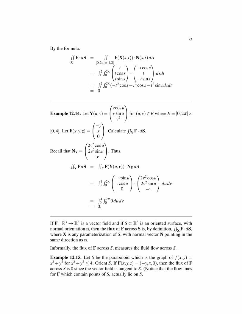
93
By the formula:∫∫X
F ·dS =∫∫
[0,2π]×[1,2]F(X(s, t)) ·N(s, t)dA
=∫ 2
1∫ 2π
0
tt cosst sins
·−t coss
t−t sins
dsdt
=∫ 2
1∫ 2π
0 (−t2 coss+ t2 coss− t2 sinsdsdt= 0
Example 12.14. Let Y(u,v)=
vcosuvsinu
v2
for (u,v)∈E where E = [0,2π]×
[0,4]. Let F(x,y,z) =
−yx0
. Calculate∫∫
Y F ·dS.
Recall that NY =
2v2 cosu2v2 sinu−v
. Thus,
∫∫Y FdS =
∫∫E F(Y(u,v)) ·NY dA
=∫ 4
0∫ 2π
0
−vsinuvcosu
0
·2v2 cosu
2v2 sinu−v
dudv
=∫ 4
0∫ 2π
0 0dudv= 0.
If F : R3→ R3 is a vector field and if S ⊂ R3 is an oriented surface, withnormal orientation n, then the flux of F across S is, by definition,
∫∫X F ·dS,
where X is any parameterization of S, with normal vector N pointing in thesame direction as n.
Informally, the flux of F across S, measures the fluid flow across S.
Example 12.15. Let S be the paraboloid which is the graph of f (x,y) =x2 + y2 for x2 + y2 ≤ 4. Orient S. If F(x,y,z) = (−y,x,0), then the flux of Facross S is 0 since the vector field is tangent to S. (Notice that the flow linesfor F which contain points of S, actually lie on S.
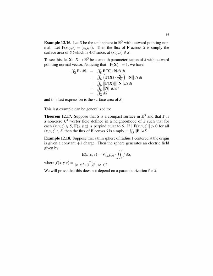
94
Example 12.16. Let S be the unit sphere in R3 with outward pointing nor-mal. Let F(x,y,z) = (x,y,z). Then the flux of F across S is simply thesurface area of S (which is 4π) since, at (x,y,z) ∈ S.
To see this, let X : D→R3 be a smooth parameterization of S with outwardpointing normal vector. Noticing that ||F(X)||= 1, we have:∫∫
X F ·dS =∫∫
D F(X) ·Ndsdt
=∫∫
D
(F(X) · N
||N||
)||N||dsdt
=∫∫
D ||F(X)||||N||dsdt=
∫∫D ||N||dsdt
=∫∫
X dS
and this last expression is the surface area of S.
This last example can be generalized to:
Theorem 12.17. Suppose that S is a compact surface in R3 and that F isa non-zero C1 vector field defined in a neighborhood of S such that foreach (x,y,z) ∈ S, F(x,y,z) is perpindicular to S. If ||F(x,y,z)|| > 0 for all(x,y,z) ∈ S, then the flux of F across S is simply ±
∫∫S ||F||dS.
Example 12.18. Suppose that a thin sphere of radius 1 centered at the originis given a constant +1 charge. Then the sphere generates an electric fieldgiven by:
E(a,b,c) = ∇(a,b,c) ·∫∫
Sf dS,
where f (x,y,z) = −1(a−x)2+(b−y)2+(c−z)2 .
We will prove that this does not depend on a parameterization for S.
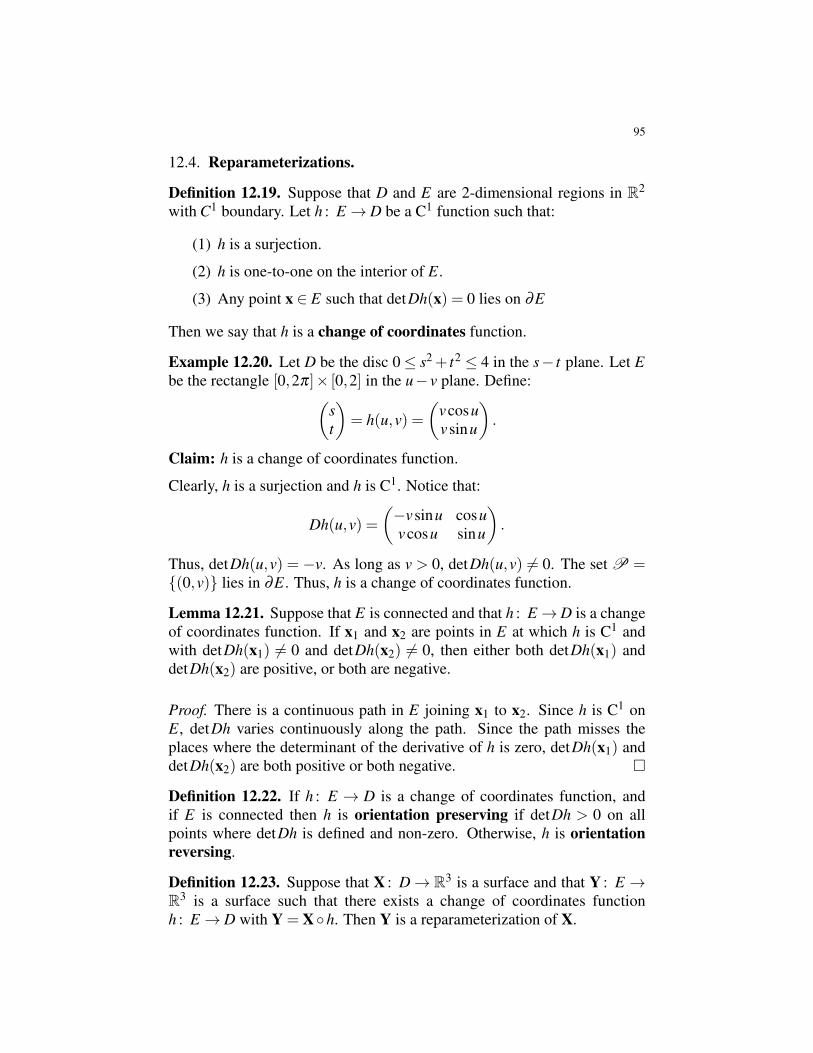
95
12.4. Reparameterizations.
Definition 12.19. Suppose that D and E are 2-dimensional regions in R2
with C1 boundary. Let h : E→ D be a C1 function such that:
(1) h is a surjection.
(2) h is one-to-one on the interior of E.
(3) Any point x ∈ E such that detDh(x) = 0 lies on ∂E
Then we say that h is a change of coordinates function.
Example 12.20. Let D be the disc 0≤ s2 + t2 ≤ 4 in the s− t plane. Let Ebe the rectangle [0,2π]× [0,2] in the u− v plane. Define:(
st
)= h(u,v) =
(vcosuvsinu
).
Claim: h is a change of coordinates function.
Clearly, h is a surjection and h is C1. Notice that:
Dh(u,v) =(−vsinu cosuvcosu sinu
).
Thus, detDh(u,v) = −v. As long as v > 0, detDh(u,v) 6= 0. The set P ={(0,v)} lies in ∂E. Thus, h is a change of coordinates function.
Lemma 12.21. Suppose that E is connected and that h : E→D is a changeof coordinates function. If x1 and x2 are points in E at which h is C1 andwith detDh(x1) 6= 0 and detDh(x2) 6= 0, then either both detDh(x1) anddetDh(x2) are positive, or both are negative.
Proof. There is a continuous path in E joining x1 to x2. Since h is C1 onE, detDh varies continuously along the path. Since the path misses theplaces where the determinant of the derivative of h is zero, detDh(x1) anddetDh(x2) are both positive or both negative. �
Definition 12.22. If h : E → D is a change of coordinates function, andif E is connected then h is orientation preserving if detDh > 0 on allpoints where detDh is defined and non-zero. Otherwise, h is orientationreversing.
Definition 12.23. Suppose that X : D→ R3 is a surface and that Y : E →R3 is a surface such that there exists a change of coordinates functionh : E→ D with Y = X◦h. Then Y is a reparameterization of X.

96
Example 12.24. Let X(s, t) =
st
s2 + t2
for 0≤ s2+ t2 ≤ 4. Let Y(u,v) =vcosuvsinu
v2
. Notice that X and Y are parameterizations of the same parab-
oloid. Define h(u,v) =(
vcosuvsinu
). Then Y is a reparameterization of X by
an orientation reversing change of coordinates.
Lemma 12.25. Suppose that X : D→R3 and that h : E→D is a change ofcoordinates function. Let Y = X◦h. Let NX and NY be the normal vectorsof X and Y respectively. Then,
NY(u,v) = (detDh(u,v))NX(h(u,v)).
Proof. We simply provide a sketch for those who have taken Linear Alge-bra. The book provides a different method.
Let S = X(D) = Y(E). Assume that both X and Y are smooth, so thatthere exists a tangent plane T Sp to S at p = X(s, t) = Y(u,v). Assume thatcoordinates on R3 have been chosen so that T Sp is the xy-plane in R3.
We think of T S(u,v) as lying in the tangent space Tp in R3 at p. Since bothX and Y are smooth, the sets of vectors {Ts,Tt} and {Tu,Tv} are each abasis for T Sp. Identifying T Sp with both the s− t plane and with the u− vplane.
By the chain rule,
DY(u,v) = DX(h(u,v))Dh(u,v).
We haveDY(u,v) =
(Tu(u,v) Tv(u,v)
)DX(h(u,v)) =
(Ts(h(u,v)) Tt(h(u,v))
)Recall that the absolute value of the determinant of a 2× 2 matrix is thearea of the parallelogram formed by its column vectors. Recall also thatdeterminant is multiplicative. Thus, by taking determinants and absolutevalues we get:
( Area of parallelogram formed by Tu(u,v) and Tv(u,v) ) =( Area of parallelogram formed by Ts(h(u,v)) and Tt(h(u,v)) )|detDh(u,v)|
Thus,||NY(u, ,v)||= ||NX(h(u,v))|| |detDh(u,v)|.

97
Since we have arranged that T Sp is the xy-plane, both NY(u,v) and NX pointin the ±k direction. That is:
NY(u, ,v) =
00
detDY(u,v)
NX(h(u,v)) =
00
detDX(h(u,v))
Since, detDY(u,v) = detDX(h(u,v))detDh(u,v), the result follows. �
Thus, if X and Y are both smooth and connected surfaces and if Y is areparameterization of X by a change of coordinates function h, then Y hasthe same normal orientation as X if and only if there exists a point (u,v)with detDh(u,v)> 0.
Example 12.26. Let X(s, t) =
st
s2 + t2
for 0≤ s2+ t2 ≤ 4. Let Y(u,v) =vcosuvsinu
v2
. Notice that X and Y are parameterizations of the same parab-
oloid. Define h(u,v) =(
vcosuvsinu
). Notice that Y = X ◦ h where h(u,v) =
(vcosu,vsinu).
Calculations show that:
NX =
−2s−2t
1
NY =
2v2 cosu2v2 sinu−v
Recalling that detDh(u,v) = −v, we see that the lemma gives us the samerelationship between NX and NY.
You may wonder how surface integrals change under reparameterization.The following theorem provides the answer:
98
Theorem 12.27. Suppose that X and Y are parameterized connected sur-faces and that Y is a reparameterization of X. If the change of coordinatefunction h is orientation-preserving, let ε = +1. If h is orientation revers-ing, let ε = −1. Let f be a C1 scalar field and let F be a C1 vector field,both defined in a neighborhood of the image of X and Y. Then:∫∫
Y f dS =∫∫
X f dS∫∫Y F · dS =
∫∫X F · dS
Proof. We will need the change of variables theorem:
Theorem. Suppose that D and E are regions in the st plane and the uvplane respectively and that h : E → D is a change of coordinates function.Let g : D→ R be C1. Then∫∫
Eg◦h |detDh(u,v)|dudv =
∫∫D
gdsdt
Both equations are a rather immediate application of this. We prove onlythe second, in the case when h is orientation reversing.
∫∫Y FdS =
∫∫E(F◦Y) ·NY dudv
=∫∫
E((F◦X)◦h) · (NX ·h)(detDh(u,v))dudv=
∫∫D(F◦X) ·NX dsdt
=∫∫
X F ·dS.The second to last equality comes from an application of the change ofvariables theorem. �

99
13. STOKES’ AND GAUSS’ THEOREMS
Definition 13.1. Suppose that S is a piecewise smooth surface which hasnormal orientation n (a unit vector). Let γ be a component of ∂S. Orient γ .We say that γ has been oriented consistently with n if it is possible to puta little triangle on γ , give the edges of the triangle arrows circulating in thedirection of the orientation of γ , use the right hand rule and obtain a normalvector pointing in the direction of n. We also say that ∂S has been given theorientation induced from the orientation of S.
Example 13.2. Suppose that A ⊂ R3 is an oriented annulus (i.e. cylinder)with two boundary components. Those boundary components must haveopposite orientations.
13.1. Stokes’ Theorem.
Theorem 13.3 (Stokes’ Theorem). Let S be a compact, oriented, piecewisesmooth surface in R3. Give ∂S the orientation induced by the orientation ofS. Let F be a C1 vector field defined on an open set containing S. Then,∫∫
S(curlF) ·dS =
∫∂S
F ·ds.
Example 13.4. Let S ⊂ R3 be the disc of radius 1 in the plane z = 1 withcenter at (0,0,1) and normal orientation pointing in the direction of the
positive z-axis. Let F(x,y,z) =
xyz
. Compute both sides of the equality in
the statement of Stokes’ theorem.
Solution: We begin with the surface integral. Let D be the unit disc in the
st-plane. We can parameterize S as X(s, t) =
st1
for (s, t) ∈ D. It is easy
to check that the normal vector for X is N(s, t) =
001
. Thus,
∫∫S
curlF ·dS =∫∫D
0dsdt
= 0
Now we calculate the line integral. The induced orientation on ∂S givesit the counterclockwise orientation when viewed from above. So we can
100
parameterize ∂S as x(t) =
cos tsin t
1
with 0≤ t ≤ 2π . Hence,
∫∂S
F ·ds =∫ 2π
0
cos tsin t
1
·−sin t
cos t0
=
∫ 2π
0 0dt= 0.
Example 13.5. Let S ⊂ R3 be the disc of radius 1 in the plane z = 1 withcenter at (0,0,1) and normal orientation pointing in the direction of the
positive z-axis. Let F(x,y,z) =
−yx0
. Compute both sides of the equality
in the statement of Stokes’ theorem.
Solution: We begin with the surface integral. Let D be the unit disc in the
st-plane. We can parameterize S as X(s, t) =
st1
for (s, t) ∈ D. It is easy
to check that the normal vector for X is N(s, t) =
001
. Thus,
∫∫S
curlF ·dS =∫∫D
002
·0
01
dsdt
=∫∫D
2dsdt
= 2π
Now we calculate the line integral. The induced orientation on ∂S givesit the counterclockwise orientation when viewed from above. So we can
parameterize ∂S as x(t) =
cos tsin t
1
with 0≤ t ≤ 2π . Hence,
∫∂S
F ·ds =∫ 2π
0
−sin tcos t
0
·−sin t
cos t0
=
∫ 2π
0 1dt= 2π.
101
Example 13.6. Let P be the paraboloid given by the equation z = x2 + y2
for x2 + y2 ≤ 1. Give P the orientation so that the normal vector to P at 0
points upward. Let F(x,y,z) be the vector field F(x,y,z) =
−yx0
. Find
the circulation of F around P.
Solution: The circulation of F around P is simply∫∫
P curlF ·dS. By Stokes’theorem this is equal to
∫∂P
F · ds. By the previous problem this is equal to
2π . (Notice that the orientation induced by P on ∂P = ∂S is the same as theorientation induced by the disc S from the previous problem.
That example generalizes to:
Theorem 13.7. Suppose that S1 and S2 are two oriented surfaces such that∂S1 = ∂S2 and such that the induced orientations on the boundary are equal.If F = curlG for some G then
∫∫S1
F ·dS =∫∫S2
F ·dS.
Proof. By Stokes’ theorem applied twice:∫∫S1
F ·dS =∫
∂S1
G ·ds =∫
∂S2
G ·ds =∫∫S2
F ·dS.
�

102
13.2. Divergence Theorem.
Theorem 13.8 (Divergence Theorem/Gauss’ Theorem). Let V be a com-pact solid region in R3 such that ∂V consists of piecewise smooth, closed,orientable surfaces. Orient ∂V with unit normals pointing out of V . Sup-pose that F is a C1 vectorfield defined on an open set containing V . Then:∫∫∫
V
divFdV =∫∫∂V
F ·dS
Example 13.9. Suppose that F is a C1 vector field defined on R3−{0} suchthat divF is a constant 7. Let S1 be the unit sphere centered at the origin andlet S8 be the sphere of radius 8 centered at the origin. Orient both S1 and S8outward. If the flux of F through S1 is 9, find the flux of F through S8.
Solution: Let V be the region between S1 and S8 and note that F is C1 on V .Giving ∂V = S1∪S2 the outward orientation gives S8 the same orientationas the one given, but gives S1 the opposite orientation. Thus∫∫
∂V
F ·dS =∫∫S8
F ·dS−∫∫S1
F ·dS.
By the divergence theorem this equals:∫∫∫V
divFdV = 7volume(V ).
The volume of V is simply 4π
3 (83)− 4π
3 = 2044π
3 . Thus,∫∫S8
F ·dS =2044π
3+∫∫S1
F ·dS =2044π
3+9.

103
14. GRAVITY
Suppose that ρ : R3→ R is a density function. That is, ρ(x) is the densityat a point x ∈ R3. If V ⊂ R3 is a 3-dimensional region, then the mass of Vis∫∫∫V
ρ dV .
The gravitational attraction exerted by a point at x on another point at r 6= xis given by:
F(r) = Gρ(x)x− r||x− r||3
where G is the universal gravitational constant.
It is easy to check that the divergence of F with respect to r is zero.
Fundamental to the study of gravitation is:
Theorem 14.1 (Gauss’ Law). Let V be a 3–dimensional region. The fluxof the gravitational field F exerted by V across ∂V is:∫∫
∂VF ·dS =−4πG
∫∫∫V
ρ dV
Proof. Simple Case: There exists a point x ∈V with ρ(x) 6= 0 and all otherpoints in V have zero density. Let S be a small sphere of radius a enclosingx contained inside V . Let n be the unit outward normal to Sa. Notice that ata point r on Sa, n(r) = (r−x)/a =−(x− r)/a.
Then ∫∫Sa
F ·dS =∫∫
SaF ·ndS
= Gρ(x)∫∫
S1a3 (x− r) · −1
a (x− r)dS= −Gρ(x)
∫∫S
a2
a4 dS= −Gρ(x)
∫∫S
1a2 dS
= −Gρ(x) 1a2
∫∫S dS
= −Gρ(x)(4π)
Now notice that since ∇r ·F = 0, by the divergence theorem, we have:∫∫∂V
F ·dS =∫∫
SF ·dS =−4πGρ(x).
The general case: For an arbitrary (integrable) density function, by super-position we have ∫∫
∂VF ·dS =−4πG
∫∫∫V
ρ dV.
�
104
We can now prove an important theorem:
Theorem 14.2 (Shell Theorem). Suppose that W is a 3–dimensional regionof constant density which is the region between a sphere of radius a≥ 0 anda sphere of radius b > a, both centered at the origin.
Then the following hold:
(1) For a point r, with ||r||> b, the force of gravity is the same as if Wwere a point mass.
(2) In either case, for a point r with a < ||r|| < b, the force of gravityvaries linearly with distance from the origin.
(3) For a point r with ||r||< a, the force of gravity is zero.
Proof. Let r be a point in R3 and let r = ||r||. By the symmetry of W , thegravitational field at r is a vector that points toward the origin. That is, ifr 6= 0,
F(r) =− f (r)rr
where f (r) is a non-negative scalar function depending only on the magni-tude r of r.
Let S be a sphere of radius r bounding a ball V centered at 0. We have:∫∫S F ·dS = f (r)
∫∫S−rr dS
= −4πr2 f (r).
By Gauss’ Law we also have:∫∫S F ·dS = −4πG
∫∫∫V
ρ dV
= −4πGmass(V ).
Thus,−4πr2 f (r) =−4πGmass(V ).
If r > b, then mass(V ) = mass(W ) and so
f (r) =Gmass(W )
r2
as desired.
If a < r < b, then the mass of V is equal to the mass of W ∩V which varieswith the cube of r. Hence f (r) varies linearly with r.
If 0 < r < b, then mass(V ) = 0 and so f (r) = 0. �