operating leverage and underinvestment: theory and...
TRANSCRIPT

1
Operating Leverage and Underinvestment: Theory and Evidence1
Chuanqian Zhang
Cotsakos College of Business, William Paterson University, New Jersey 07470
Email: [email protected]
Feng Jiao
University of Lethbridge, Canada
Email: [email protected]
Xiaoyu Zhang
Shanghai University of Economics and Finance, China
Shanghai Pudong Development Bank (SPDB)
Email: [email protected]
Michi Nishihara
Graduate School of Economics, Osaka University, Toyonaka, Osaka 560-0043, JAPAN
Email: [email protected]
1 We thank Marc Arnold for his constructive suggestions. Part of this work was conducted when Zhang visited Osaka
University and he thanks for their accommodation.

2
Operating Leverage and Underinvestment: Theory and Evidence
Abstract
Operating leverage, caused by fixed operating cost, is normally considered as an internal debt of corporates. We
explore its implication on firms’ investment decision. A simple contingent-claims model delivers an appealing
fact that although operating leverage alone deters investment, it can, jointly with financial leverage, accelerate
investment timing. In Myers’ (1977) theory, the default risk caused by existing corporate bond induces the
underinvestment (or debt overhang) problem because a fraction of new project value will be transferred from
equity holders to debt holders. We show that the fixed operating cost mitigates such agency conflicts via a reverse
wealth transfer and improves investment efficiency. Using a proportional hazard model implemented on a large
sample of publicly traded U.S. firms over the period 1966-2016, the results offer strong support to our model-
based predictions. These empirical findings still hold when various measures of operating leverage are taken care.
JEL Classification: G31
Keywords: Structural model, Operating leverage, Corporate investment, Debt overhang

3
1. Introduction
It has been well established that financial leverage can cause debt overhang problem because equity holders worry
a wealth transfer from themselves to debt holders at investment. However, though in a similar payment pattern,
operating leverage has been drawn far less attentions in its relationship to a firm’s investment decision. Perhaps it
is due to conventional wisdom that fixed operating cost erodes prospective profit margin thus it should reduce
investment activities. We, despite its simplicity, argue that such intuition is unable to disclose the full story since
it neglects an interaction between these two types of leverages, given the fact that both of them usually co-exist
during firms’ operation. Thus in this article we prepare to bridge this gap by addressing the following question:
How will the joint effect of operating and financial leverages shape a firm’s investment decision?
To this end, we build a structural model in a real options setting. The model is fully dynamic since the firm’s
value and decisions are governed by a single variable, market demand, which evolves in a diffusive process. The
firm has an expansion opportunity to increase its current production capacity to a higher level. An operating cost
is necessitated to sustain the production. It is quasi-fixed because it grows in proportion to the size of capital stock
while be independent of the sales, giving rise to operating leverage as market demand fluctuates. Prior to
investment, the equity holders have an existing console bond which incurs period constant coupon. Debt renders
the firm risky since if the firm were unable to generate enough cash flows, either by profitable production or
issuing new equity, to cover the interest payment, it will go bankruptcy. Once the bankruptcy trigger is hit before
investment happens, the debt holders are assumed to taken over all unlevered assets, whose value largely depend
on future sales and operating cost. When the market demand is sufficiently low, the debt holders have to liquidate
the capital stock with zero value. The equity holders’ goal is to choose optimal investment and default thresholds
to maximize their ex ante market value.

4
In line with Myer’s (1977) theory, exercising growth options lead to augmented revenue flow and reduced
uncertainty2 that renders existing debt safer and introduces wealth transfer from equity holders to debt holders.
Expecting this, equity holders will bypass some projects with positive NPV causing underinvestment. Therefore
underinvestment problem only matters for unsecured debt. On the other hand, the fixed operating cost, largely
overlooked by current literatures, also increases the burden on shareholders’ liability side especially when
economy is at downturn, inducing a higher bankruptcy threshold. However, the operating leverage differs from
financial leverage in the sense that the former introduces liquidation risk to unlevered asset while the later causes
bankruptcy or credit risk for levered assets. At the time of default, the liquidation risk will be delegated to debt
holders when they take over the production capital, namely, a risk-shifting effect which neutralize
underinvestment problem. With that being said, the operating leverage can be considered as an “internal debt”.
In summary, our model produces following testable outcomes. First, similar to financial leverage, operating
leverage also has negative impact on corporate investment to the extent that investment timing increases with the
fixed operating cost. Second, the joint effect of the two types of leverages has positive impact on investment. To
be specific, when the operating cost is relatively low, the investment trigger increases monotonically with
financial leverage; when the operating cost is relatively high, the investment trigger presents a slightly U-shaped
or even decreasing relationship with financial leverage. To aid the analysis, we also quantify the corresponding
agency conflicts between debtholders and shareholders. It shows that the magnitude greatly declines as operating
leverage increases.
Guided by model generated predictions, we test them empirically. It is noteworthy that although operating
leverage is straightforward in terms of definition, it is probably less straightforward to proxy in empirics since
quasi-fixed operating cost is difficult to observe. Therefore we employ three typical measures of operating
leverage from García‐ Feijóo and Jorgensen’s (2010), Novy-Marx(2011) and Chen, Harford and Kamara (2017)
respectively. Then we carry out empirical test using a large panel data covering 16,169 publicly traded firms over
2 Growth options represent contingent claims to future payoffs thus they are exposed to more uncertainty than the present
value of those payoffs (i.e. post-investment asset-in-place).
5
the period from 1966 to 2016. After estimating a mixed proportional hazard model, as in Leary and Roberts
(2005), Whited (2006) and Morellec, Valta, and Zhdanov (2015), we demonstrate that either financial leverage or
operating leverage does hinder corporate investment, and operating leverage weakens the negative relationship
between financial leverage and investment, consistent with our model predictions. These findings still hold when
alternative measures of operating leverage and financial leverage are employed. In addition, we also consider
potential endogeneity pertaining to the financial leverage and the operating leverage: 1) we attempt to address the
endogenous concern between financial leverage and investment by using the instrumental variable approach
(Tchetgen et al. ,2015; Sunder et al, 2017); 2) we perform industry-level estimations as a robustness check, since
the potential for endogeneity of operating leverage is much less severe at the industry level.
Our paper is related two strands of literatures. First, we contribute to related theoretic works on identifying
determinants of underinvestment problem due to agency cost of debt overhang. For example, previous works
have investigated an array of financial leverage-side (or external debt) factors such as debt renegotiation by
Pawlina (2010), debt priority structure by Hackbarth and Mauer (2012), short-term debt by Diamond and He
(2014). We complement their work by revoking the impact of operating leverage (or internal debt) which is
ignored by those papers. Arnold et al. (2017) find that investment financed by asset sales can mitigate debt
overhang within aggregate dynamics. Hirth and Uhrig-Homburg (2010) reveal that cash financed investment can
completely eliminate debt overhang problem. Both of them essentially show a reverse wealth transfer process due
to exchanging riskless asset for risky assets upon investment. Our model reveal a similar result but distinguishes
from them in terms of mechanism, namely, a liquidation risk transition from equity holders to debt holders
through operating cost embedded in unlevered assets.
Second, our paper contributes to the research field related to operating leverage or cost structure in both
theory and empirics. The operating leverage has been extensively investigated in asset pricing literatures3 in
recent years while only a few relates it to corporate policies. Among them Chen et al (2017) explore the
3 See Carlson, Fisher and Giammarino (2004), Hackbarth and Johnson (2015), Gu, Hackbarth and Johnson (2018),
Bustamante and Donangelo (2016), Novy-Marx (2011), García-Feijóo and Jorgensen (2010)

6
substitution and interaction effect between operating leverage and financial leverage on the components of
profitability. Kulchania (2016) explores the impact of cost structure on firms’ payout policy. We complement
their work by focusing on the interplay between the two leverages on corporate investment. Perhaps the closest
one to ours, Kumar and Yerramilli (2017) study the substitution between the two types of leverages on
endogenous capital structure and capacity choice. We complement their work by concentrating on investment
timing and providing intriguing empirical evidence.
The rest of paper proceeds as follows: Section 2 develops model frameworks as well as their numerical
solutions. Then we derive testable hypothesis based on the results. Section 3 introduces data and empirical design.
Section 4 presents empirical findings. Section 5 concludes the paper.
2. Model settings
2.1 Two-period Example
We set up a static model bearing resemblance to Diamond and He (2014) within a context of capacity expansion.
However, we augment their work by considering quasi-fixed operating cost, which only varies in a proportion to
the size of installed capital instead of sales. At the beginning t = 0 the firm has already installed capital stock of 𝐾
and it will not generate cash flows until the ending period t = 2.
The equity holders will immediately liquidate their production capital with zero value if the profit flow is
negative. The firm has already raised zero-coupon bond with face value F at t = 0 and the debt will be retired at t
t = 1
𝐾(𝑥 − 𝑚), investment 𝐾(𝑥 − 𝑚), no investment
𝐾(𝑦 − 𝑚), investment 𝐾(𝑦 − 𝑚), no investment
t = 2,
debt matures
t = 0
issue debt
1
2
1
2
𝐺 𝐵
p p

7
= 2. Managers will also need to make investment decision right after debt issuance. The economy can be evolved
to two status at t = 1, namely, Good (G) and Bad (B) with equal opportunity ½. Without any investment, the
deployed assets could generate revenue per capital x and y with x > y in either economic status. The asset in place
is procyclical in the sense that p > 1/2. That is to say chances are higher for firms generate high sales than
generate low sales at good time. Note we also could generalize the setting by differentiating pG and pB but it will
complicate the analysis while deliver same results. Once the firm conducts investment the capital size increases
from 𝐾 to 𝐾 in exchange for cost 𝑘∆, with Δ = 𝐾 − 𝐾.
The debt is risky such that 𝐾(𝑥 − 𝑚) ≥ 𝐹 ≥ 𝐾(𝑦 − 𝑚). When profit flows are not enough to pay back to
debt holders, the equity holders declare bankruptcy. The Absolute Priority Rule is implemented hence equity
holders seize zero value while debt holders receive all realized cash flows. The discount rate is set to zero. In what
follows we analyze investment criteria as well as associated agency cost given the assumption that the investment
is made at t = 0 thus the firm is unaware of future economic status and cash flow distributions. Later on we redo
the analysis for investment decision being made at t = 1, at which the economic status is disclosed. Since we wish
to explore the interactive effect of operating leverage and financial leverage, the analysis is separated two cases:
low and high operating cost. For each case, we derive solution for both low and high debt levels.
Case A: when the quasi-fixed operating cost is relatively low m < y and
(1) If financial leverage is relatively low, 𝐾(𝑦 − 𝑚) ≥ 𝐹, the value of equity holders who make investment will
be 𝐸𝐻 =1
2𝐾(𝑦 − 𝑚) +
1
2𝐾(𝑥 − 𝑚) − 𝑘∆ − 𝐹;
(2) If financial leverage is relatively high, 𝐾(𝑦 − 𝑚) ≤ 𝐹, the equity value of firm who makes investment will be
𝐸𝐿 =1
2𝐾(𝑥 − 𝑚) − 𝑘∆ −
1
2𝐹.
On the other hand, if the firm doesn’t undertake any investment the equity value will become 𝐸 =
1
2𝐾(𝑥 − 𝑚) −
1
2𝐹. Thus the investment criteria will be:
(1) For low financial leverage, the investment will be initiated only if 𝐸𝐻 > 𝐸 or 𝑥 ≥ 2𝑘 + 𝑚 +𝐹−𝐾(𝑦−𝑚)
∆.
Note the last item on the right hand side is negative.

8
(2) For high financial leverage, the condition for investment is 𝐸𝐿 > 𝐸 or 𝑥 ≥ 2𝑘 + 𝑚
It can be easily detected that investment is more likely for low-debt firm since the criteria is less binding. In
addition, as operating cost m increases, the investments for both scenarios are harder to realize, consistent with
conventional wisdom. In terms of agency cost, we measure it as the foregone investment opportunities. For
instance, at low debt level, the agency cost is zero while at high debt level, the agency cost will be 𝐴𝐶 =
1
2∆(𝑥 − 𝑚 − 𝑘) , which declines with m.
Case B: when the operating leverage is relatively high m ≥ y, the equity holders will close production with
scrap value of zero at bottom knot of t = 2, regardless of debt amount. Therefore the equity value of firms
undertaking investment will be 𝐸𝐻 = 𝐸𝐿 =1
2𝐾(𝑥 − 𝑚) − 𝑘∆ −
1
2𝐹. Thus the corresponding threshold is always
hold at 𝑥 ≥ 2𝑘 + 𝑚, namely, there is no underinvestment problem.
In summary the model illustrates that operating leverage can mitigate underinvestment problem, especially
for firms financed with relatively high debt. In the next, we corroborate the main implication by assuming an
alternative scenario that the firm makes investment decision at t = 1. The stepwise derivation will not be shown
since it is same as previous case.
At point G, when operating cost is low m < y, the investment conditions are 𝑥 ≥ 𝑘/𝑝 + 𝑚 for high financial
leverage and 𝑥 ≥𝑘
1−𝑝+ 𝑚 −
1−𝑝
𝑝∆[𝐾(𝑦 − 𝑚) − 𝐹] for low financial leverage. It can be easily observed that the
latter is less binding than former one. Alternatively, when operating leverage is high m > y the two investment
criteria are identical. The agency cost (only applicable for low operating leverage) is = 𝑝∆(𝑥 − 𝑚 − 𝑘) . At
point B, all results are same as in point G, except for replacing p with 1 – p.
Again, the solutions to the second investment pattern lend further support to our main result. In what follows,
we generalize the setting in a dynamic world.
2.2 Dynamic model
9
Consider a firm operates in a continuous-time, infinite-horizon, and partial-equilibrium economy with decreasing
to scale technology4 incorporated in the Cobb-Douglas production function. The installed capital stock generates
the profit flow which can be expressed as
𝜋𝑡 = 𝑥𝑡𝐾𝑡𝛾
− 𝑚𝐾𝑡
In this equation, γ < 1 denotes the return to economic scale and m represents cost of operating the
production capital K. Since we assume the capital is at steady state and depreciation is excluded thus we have
𝐾𝑡 ≡ 𝐾. The variable x concisely captures market demand level which evolves Geometric Brownian Motion
(GBM) process in a risk-neutral measure, namely
𝑑𝑥 = 𝜇𝑥𝑑𝑡 + 𝜎𝑥𝑑𝑍
where μ and σ are positive constants, and (Zt)t ≥0 is a standard Brownian Motion Process. Time is continuous
and varies over [0, ∞). Uncertainty is represented by the filtered probability space (𝛺, ℱ, (ℱ𝑡)𝑡≥0, ℙ) over which
all stochastic processes are defined. The firm is subjected to a constant corporate tax rate of τ (0< τ <1).
Investment Opportunity: At any time, the firm may exercise expansion option to increase its capital stock.
Define the constant capital level before investment as 𝐾 and the augmented capital level as 𝐾 which obeys 𝐾 >
𝐾. To implement it, the firm will pay an investment cost 𝑘(𝐾 − 𝐾) in exchange for receiving enhanced assets
scale and k can be viewed as purchasing price of unit capital. We assume this investment cost is financed by
common equity and abstract from debt financing, in line with recent related works such as Arnold et al. (2017)
and Chen and Manso (2017)5 because the main topic of our paper is investigating the underinvestment problem.
As mentioned in Arnold et al. (2017), this assumption is justifiable for firms that have existing debt embedded a
covenant prohibiting them to raise new debt.
4 The decreasing to scale technology has been widely applied such as Chen, Harford and Kamara (2016), Hackbarth and
Johnson (2015), etc. 5 Other underinvestment models such as Mauer and Ott (2000), Pawlina (2010) and Hirth and Uhrig-Homburg (2010) apply
similar assumption.

10
Bankruptcy: The firm may declare bankruptcy either before or after the investment decision is made. If
default occurs prior to investment, debt holders will receive the firm’s assets in place and the unexercised
investment option subtracted by a fractional bankruptcy cost of φ, and equity holders will receive nothing (i.e.,
absolute priority rule, or APR, is enforced). If the firm declares bankruptcy after the investment, the debt holders
will also similarly receive present value of unlevered assets, subtracting the same bankruptcy cost φ. We assume
debt holders are not allowed to lever up the residual assets afterwards, consistent with the contingent-claim
literature (Leland, 1994, Mauer and Ott, 2000). The alternative bankruptcy process such as debt renegotiation/
restructure can also be applied but it will not change the conclusion while complicate the analysis.
Operating leverage: As in Novy-Marx (2011) we directly adopt unit operating cost m as a measure of
operating leverage in our model since it not only concisely reflects the quasi-fixed nature but also relates closely
to our empirical measures. Notably, in related literatures, the operating leverage might be expressed in other
alternative ways. For example, Gu, Hackbarth and Johnson (2018) defines operating leverage as operating cost
over sales revenue. Bustamante and Donangelo (2017) interpret operating leverage as operating cost divide
operating profit. We believe those variations are of minor importance since they are monotonic functions of m.
The empirical proxies of m will be introduced in section 3.2.
The model is solved in two parts: we first derive the unlevered firm value and associated investment decision
then we solve the levered firm value and corresponding investment and bankruptcy decisions. For each part, the
model is solved in a backward manner. That is, we first solve each contingent claims given investment has been
exercised than we solve their counterparts prior to investment.
2.2.1 Unlevered firm:
After investment, the unlevered firm's asset value is no more than a present value of discounted cash flow plus a
contraction option
𝑉1
𝑢(𝑥) = (1 − 𝜏) (𝑥𝑡𝐾
𝛾
𝑟−𝜇−
𝑚𝐾
𝑟) + 𝐵𝑥𝛽 (1)

11
in which parameter β is the negative root of the quadratic equation: 1/2𝜎2𝛽(𝛽 − 1) + 𝜇𝛽 − 𝑟 = 0. To solve eq (1)
we need extra conditions 𝑉1𝑢(𝑥𝐿) = 0 and
𝜕𝑉1𝑢(𝑥𝐿)
𝜕𝑥= 0, where xL is the liquidation threshold. There is a closed
form solution for both liquidation threshold and firm value
𝑥𝐿 =𝛽
𝛽−1
𝑟−𝜇
𝑟
𝑚𝐾
𝐾𝛾 (2)
𝑉1𝑢(𝑥) = (1 − 𝜏) [
𝑥𝑡𝐾𝛾
𝑟−𝜇−
𝑚𝐾
𝑟− (
𝑥𝐿𝐾𝛾
𝑟−𝜇−
𝑚𝐾
𝑟) (
𝑥
𝑥𝐿)
𝛽] (3)
Before investment the firm value can be written as
𝑉0𝑢(𝑥) = (1 − 𝜏) (
𝑥𝑡𝐾𝛾
𝑟−𝜇−
𝑚𝐾
𝑟) + 𝐻1𝑥𝛼 + 𝐻2𝑥𝛽 (4)
where H1 and H2 are unknown constants, α is the positive root of the quadratic equation: 1/2𝜎2𝛽(𝛽 − 1) + 𝜇𝛽 −
𝑟 = 0. To solve the optimal investment trigger x* we need following conditions (similar to static model, we use
𝛥 = (𝐾 − 𝐾) to represent increased amount of capital)
𝑉(𝐾, 𝑥∗) = 𝑉(𝐾, 𝑥∗) − 𝑘𝛥 (5)
𝜕𝑉(𝐾,𝑥)
𝜕𝑥|
𝑎𝑡 𝑥=𝑥∗=
𝜕𝑉(𝐾,𝑥)
𝜕𝑥|
𝑎𝑡 𝑥=𝑥∗ (6)
Eq (5) is value matching condition to ensure value equivalence at investment and eq (6) is smooth pasting
condition that guarantees optimality of investment timing. Since the firm could exit at distress prior to investment
we have boundary conditions at pre-investment liquidation trigger 𝑉1𝑢(𝑥𝐼𝐿) = 0 and
𝜕𝑉1𝑢(𝑥𝐼𝐿)
𝜕𝑥= 0. Now we
present valuation and investment decisions for firms with debt financing:
2.2.2 Levered firm
In this section, we assume the managers act in the interest of equity holders and make investment decision to
maximize pre-investment equity value. We call it second-best strategy as opposed to first-best strategy, in which
managers make investment decision to maximize firm value.
Using similar technique, the post-investment equity and debt value can be derived as follows

12
𝐸1(𝑥) = (1 − 𝜏) [𝑥𝑡𝐾
𝛾
𝑟−𝜇−
𝑚𝐾+𝑐
𝑟− (
𝑥𝑏1𝐾𝛾
𝑟−𝜇−
𝑚𝐾+𝑐
𝑟) (
𝑥
𝑥𝑏1)
𝛽] (7)
𝐷1(𝑥) =𝑐
𝑟+ [(1 − 𝜑)𝑉1
𝑢 −𝑐
𝑟] (
𝑥
𝑥𝑏1)
𝛽 (8)
in which the optimal post-investment default trigger is analytically obtained 𝑥𝑏1 =𝛽
𝛽−1
𝑟−𝜇
𝑟
𝑚𝐾+𝑐
𝐾𝛾
Then we present pre-investment firm value:
𝐸0(𝑥) = 𝐴1𝑥𝛼 + 𝐴2𝑥𝛽 + (1 − 𝜏) (𝑥𝑡𝐾𝛾
𝑟−𝜇−
𝑚𝐾+𝑐
𝑟) (9)
𝐷0(𝑥) = 𝐵1𝑥𝛼 + 𝐵2𝑥𝛽 +𝑐
𝑟 (10)
where A1, A2, B1, B2 are constants to be solved. We also need to address optimal default xb0 and investment
threshold x*. To do this, we recall both value matching (eq 11) and smooth pasting (eq 12) conditions at
investment threshold x*
𝐸0(𝑥∗) = 𝐸1(𝑥∗) − 𝑘𝛥 (11)
𝜕𝐸0(𝑥)
𝜕𝑥|
𝑎𝑡 𝑥=𝑥∗=
𝜕𝐸1(𝑥)
𝜕𝑥|𝑎𝑡 𝑥=𝑥∗
(12)
Note the eq (12) captures the idea of “second-best” policy that firms follow equity-maximizing investment
decision. To solve bankruptcy threshold prior to investment, we need following conditions at default threshold
𝐸0(𝑥𝑏0) = 0 and 𝜕𝐸0(𝑥)
𝜕𝑥|𝑎𝑡 𝑥=𝑥𝑏0
= 0 (13)
To solve B1 and B2 we use conditions:
𝐷0(𝑥∗) = 𝐷1(𝑥∗) (14)
𝐷0(𝑥𝑏0) = (1 − 𝜑)𝑉0𝑢(𝑥𝑏0) (15)
Both eq (14) and (15) are value matching conditions: the first one demonstrates that the pre- and post-investment
debt value should be identical since there is no new debt issued. The second one is from assumption that debt
holders get unlevered assets subtracted from bankruptcy cost.
2.2.3 Results of benchmark model
13
We define the benchmark model as the one that abstracts from corporate tax and bankruptcy cost. It serves two
purposes. First, we aim to make it fully comparable with that of static model which ignores two of them. Second,
it is attractive since the severity of underinvestment will be purely driven by agency conflicts. However, this
assumption might also make the incentive to issue debt ungrounded thus we relax it in the next section. Notice
that given there is no tax and bankruptcy cost, the optimal investment of an unlevered firm is equivalent to that of
debt-financed firms pursuing first-best strategy (a formal proof is shown in Appendix A).
The economic-wide parameter values are used in line with Hackbarth and Mauer (2012): the risk-free interest
rate r = 6%, volatility of market demand σ = 25%, expected growth rate of demand μ = 1%. For the economic
return to scale, we set γ = 0.8, which is in between Whited (2006, γ = 0.75) and Gu et al. (2017, γ = 0.85). The
purchasing cost per unit capital k = 3 without loss of generality. The initial market demand x0 = 0.87 which
ensures the firm is alive but has not invested at t = 0, the initially installed capital 𝐾 = 1 and augmented capital
𝐾 = 2.
Figure 1(a) illustrates relationship between investment trigger and coupon payments. The solid line
represents firms operating with low cost (m = 0.2) in which the investment trigger increases from 0.77 to 0.93 as
coupon increases from 0 to 1.2. The dash dotted line graphs firms operating with medium cost (m = 0.5) and the
investment trigger decreases from 1.42 to 1.36 and then increases to 1.40. The dotted line is meant to firms
operating with high cost (m = 1.2) and the investment trigger decreases monotonically from 2.89 to 2.68. In real
option terms, a higher trigger implies low possibility that the investment will be conducted. In line with this logic,
Fig 1(b) graphs ex ante investment probability given no bankruptcy has yet to come6. It can be observed that the
probability for lowest operating cost decreases by 26.5% (from 93.5% to 67%) while for highest operating cost
decreases by 19.5% (from 20% to 0.05%). In summary the numerical results demonstrate that the negative impact
of financial leverage on investment is greatly mitigated and even reversed as the operating cost increases.
6 The probability of investment given no bankruptcy has not happened can be written as 𝑝(𝑥0) =𝑥0
2𝜆/𝜎2−𝑥𝑏0
2𝜆/𝜎2
𝑥𝐼2𝜆/𝜎2
−𝑥𝑏02𝜆/𝜎2 with 𝜆 =
−(𝜇 − 𝜎2/2), the detailed derivations are in Hackbarth and Mauer (2012)

14
[Figure 1 insert here]
The suboptimal investment implied from Fig 1 indicates an agency cost between equity and debt holders. To
visualize the magnitude, Figure 2 demonstrates further the relationship between agency cost and coupon payments
for a range of operating leverage. The agency cost is calculated by quantifying difference of pre-investment firm
values pursuing first-best and second-best strategies. The solid line represents firms operating with low cost (m =
0.2) in which the agency cost increases from 0 to 0.4% as coupon increases from 0 to 1.2%. The dotted line and
dashed line graphs for firms with medium operating cost (m = 0.4) and high operating cost (m = 1.2) respectively,
however, their magnitude declines significantly compared to that of low operating cost.
[Figure 2 insert here]
To lend more support to our model-based results, we also perform several comparative studies. Specifically,
we investigate if the main results are still valid by varying key parameters such as return to scale γ, cash flow
volatility σ, and growth multiple 𝐾/𝐾. Because they are normally believed to impact debt overhang problems.
For example, a higher return to scale and cash flow volatility or lower growth option will mitigate debt overhang,
which might contaminate our operating leverage channel. The results are depicted at Appendix B.
2.2.4 Impact of Tax and Bankruptcy cost
In this section we continue to follow Hackbarth and Mauer (2012) to adopt tax rate τ = 15% and bankruptcy
filing cost φ = 25%. The investment decision for firms pursuing first-best strategy can be computed from an
alternative smooth pasting condition
𝜕(𝐸0(𝑥)+𝐷0(𝑥))
𝜕𝑥|𝑎𝑡 𝑥=𝑥∗
=𝜕(𝐸1(𝑥)+𝐷1(𝑥))
𝜕𝑥|𝑎𝑡 𝑥=𝑥∗
(16)
All other boundary conditions are same as in aforementioned. We first analyze investment decision through
comparing high (m = 1.2) and low (m = 0.3) operating costs. Specifically, the dotted line captures investment
trigger for first-best (FB) scenario while the solid line represents second best (SB) scenario. To highlight their
numerical significance, we report following result: for high operating cost, the FB investment trigger keeps
relatively flat (ranges from 3.18 to 3.17) whereas the SB trigger decreases monotonically from 3.18 to 3.02; for

15
low operating cost, the FB investment trigger decreases from 1.25 to 1.13 whereas the SB trigger increases from
1.25 to 1.34. Converting to probabilities, fig 4(b) shows that, when firms pursue SB strategy, the high operating
cost case decreases by around 26% (from 72.3% to 46.6%) whereas the low operating cost case declines by
around 19% (from 19.6% to 0.04%). Notice that the investment probabilities are almost same for FB and SB
decisions for firms with high operating cost case, indicating a disappearing agency cost as financial leverage
increases.
[Figure 4 inserts here]
Figure 5 illustrates agency cost for those two different operating leverage cases. The agency cost is obtained
by valuing 𝐴𝐶% =𝑉𝐹𝐵(𝑥0)−𝑉𝑆𝐵(𝑥0)
𝑉𝐹𝐵(𝑥0)× 100, in which 𝑉𝐹𝐵 and 𝑉𝑆𝐵 represent the firm value under first and second
best investment policy. For high operating cost case the agency cost increases from 0 to 0.41% while for low
operating cost case the agency cost shows a slightly bump shape with significantly smaller magnitude.
The classic tradeoff theory indicates that there exists an optimal debt level given tax and default cost. Thus
we also calculate the optimal coupon as well as agency cost by varying a range of operating costs. However, it
deserves attention that the optimal financial leverage ratio is less relevant in empirics since the debt ratio usually
deviates from the optimal level due to either adjustment cost or agency cost of debt overhang (Chen and Manso
2017),, Thus in our paper we believe an exogenous range of debt level connects model setting with empirics in a
better way. Fig 6 (a) plots the optimal coupon with a variety of operating cost. It shows that the results for FB and
SB have been converged when the operating cost is approximately larger than 0.3 and their difference is enlarged
as operating cost decreases when debt overhang effect dominates. Fig 6(b) calibrates agency cost by assuming an
optimal coupon has been embodied in both FB and SB cases. It shows that agency cost could be completely
eliminated when operating cost is around 0.43.
In summary, a full-fledged numerical computation indicates following testable hypothesis
H1: All else being equal, a firm’s optimal investment timing will be postponed with either financial leverage
or operating leverage.
H2: The joint effect of the two leverages has positive impact on the investment timing or probability.

16
Statistically, to test the investment timing is equivalent to test the associated hazard rate of an investment,
namely the probability of exercising an investment today as a function of the time since the last project. On the
contrary, accounting data always presents a continuous investment pattern across periods. Thus we follow Whited
(2006)7 to count project investment only if a firm invests as twice as much the historic mean.
3. Empirical Design
3.1. Data
Our primary data comes from Standard & Poor’s COMPUSTAT database available on the Wharton Research
Data Services server. We draw a sample of firm-year observations for the period 1966 to 2016. We include firms
that are located and incorporated in the United State. To maintain consistency with previous empirical literature,
we exclude regulated utility firms (SIC codes between 4900 and 4999) and financial firms (SIC codes between
6000 and 6999), as well as government entities (SIC codes greater than or equal to 9000). We exclude all
observations for which the total book value of assets or net sales is either missing or negative.
After excluding missing observations for all related variables, we get the final data set with 143,109 unique
firm-years for 16,169 publicly traded firms. For robustness check, we use book leverage as an alternative measure
of firm leverage. This results in a smaller dataset with 138,497 firm-year observations. Appendix B contains
definitions of the variables used in the analysis.
3.2. Measures of Operating Leverage and Other Variables
Although operating leverage is straightforward in terms of definition, it is probably less straightforward to proxy
in empirics since quasi-fixed operating cost is difficult to observe. So far there are several proxies for operating
leverage in the extant studies. We measure operating leverage by adopting three typical variables respectively.
First, we follow the empirical approach of García‐ Feijóo and Jorgensen’s (2010) who estimate the annually time-
varying degree of operating leverage (DOL) by running the time-series regressions at five-year overlapping
7 In recent literatures the hazard function has been applied to empirical test of investment timing in a real options framework
such as Morellec et al (2015) and Akdoğu and Mackey (2008), etc.

17
intervals at firm-level. We estimate the DOL using a two-step time-series regression approach. First, we run
regressions below over five-year overlapping intervals for each individual-firm:
Ln𝐸𝐵𝐼𝑇𝑡 = 𝑔𝑒𝑏𝑖𝑡t + Ln𝐸𝐵𝐼𝑇𝑖0 + 𝛿𝑒𝑏𝑖𝑡,𝑡
Ln𝑆𝑎𝑙𝑒𝑠𝑖𝑡 = 𝑔𝑠𝑎𝑙𝑒𝑠t + Ln𝑆𝑎𝑙𝑒𝑠𝑖0 + 𝛿𝑠𝑎𝑙𝑒𝑠,𝑡
where EBIT0 and Sales0 are the beginning levels of earnings before interest and taxes (EBIT) and Sales,
respectively. Next, we run the following regression on the residuals 𝛿𝑒𝑏𝑖𝑡,𝑡 and 𝛿𝑠𝑎𝑙𝑒𝑠,𝑡:
𝛿𝑒𝑏𝑖𝑡,𝑡 = 𝛾0𝑖 + 𝛾1𝑖𝛿𝑠𝑎𝑙𝑒𝑠,𝑡 + 𝑢𝑖𝑡
Where the regression coefficient 𝛾1𝑖 is the estimator of DOL for company i. 𝑢𝑖𝑡 is error term. The time period for
the regression runs from 1966 to 20168. Here to deal with negative values in the above estimation, we use the
transformation technique adopted by García‐ Feijóo and Jorgensen’s (2010), which is also common in accounting
research (Ljungqvist and Wilhelm, 2005). The transformation is given in the below.
Y=Ln(1+X), if X≥0 and Y=-Ln(1-X), if X<0
Where X stands for EBIT, Sales and Y is the value of the natural logarithm of the two variables after the
transformation9.
Next, we adopt the proxy used by Novy-Marx(2011), which is calculated as the sum of cost of goods sold
(COGS) and selling, general, and administrative expenses (XSGA) scaled by total assets. This measure can
capture the variable production costs well.
In addition, similar to the empirical proxy used by Novy-Marx(2011), we adopt the proxy used in Chen,
Harford and Kamara (2016) and calculate operating leverage as selling, general, and administrative expenses
(XSGA) divided by total assets. Different from Novy-Marx(2011), they don’t include cost of goods sold (COGS)
8 For example, the DOL for year 1966 is estimated by time- series regression over fiscal years 1962-1966; the DOL for year
1967 is estimated by time- series regression over fiscal years 1963-1967 so on so forth. Thus the real time window for the
data is 1962 to 2016. 9 The adjusted value of LnEBIT and LnSales are used hereafter thus these are values after the adjustment rather than the
natural logarithm of original data.

18
in the numerator for two reasons. First, XGSA is much stickier than COGS. Compared with XSGA, it is much
more responsive to fluctuations in sales and so is better characterized as variable costs. Second, the exclusion of
COGS helps mitigate potential endogeneity concerns. COGS depends on the production of goods and therefore,
the inclusion of COGS makes firm’s operating leverage dependent on production.
As for financial leverage, we firstly compute it as the ratio of total debt scaled by the sum of total debt and
total shareholders’ equity at the end of the year (see Fang, Huang and Karpoff (2015)). In order to show that these
results are not driven by specific measure of this variable, we also compute financial leverage as book leverage,
that is, the ratio of total debt divided by total assets for robustness (Valta, 2012).
As for the measure of investment, most studies measure firm-specific investment intensity by capital
expenditures scaled by either total assets (Mayers, 1998, Korkeamaki and Moore, 2004), or property, plant, and
equipment (PP&E) (Fazzari, Hubbard, and Petersen, 1988, Hoshi, Kashyap, and Scharfstein, 1991). We focus on
capital expenditures divided by PP&E at the beginning of the year. Since a majority of firms in our sample invests
at least a small amount every year, the definition of a large project investment requires future adjustment (Whited,
2006). Low observed level of investment intensity might occur simply because of maintenance. Following Whited
(2006) and Morellec, Valta, and Zhdanov (2015), we adopt the measure of investment spike as our primary
dependent variable. An investment spike occurs if the ratio of investment to total assets is two times greater than
the firm median. In our sample, we observe 20,606 investment spikes, approximately 14.4% of our total
observations. The proportion is similar to those reported by Morellec, Valta, and Zhdanov (2015) and Whited
(2006).
We include several control variables in our estimations that were proven to affect firm investment in the
literature. They include Tobin’s Q, size, cash flow, sales growth rate, tangibility, R&D, cash flow volatility,
dividend, and cash holdings. The variable definitions are provided in Appendix B, and Table 1 provides summary
statistics for all the variables.
3.3. Empirical Specification

19
We estimate a mixed proportional hazard model, as in Leary and Roberts (2005), Whited (2006) and Morellec,
Valta, and Zhdanov (2015), to examine the effects of operating leverage on investment. The hazard function at
time t for firm i with covariates Xi(t) is
𝛾𝑖(𝑡) = 𝜔𝑖𝛾0(𝑡)exp (𝑿𝒊(t)′𝜷)
where t is the time to investment, 𝛾0(𝑡) is the baseline hazard, wi is a random variable that represents unobserved
cross-sectional heterogeneity. Xi(t) is a vector of covariates, is the corresponding vector of coefficients we need
to estimate. The Xi(t) and allow “the hazard to shift up and down depending on their values” (Whited, 2006).
We estimate the mixed proportional hazard model using maximum likelihood. We consider two specifications of
covariates.
First we set the term Xi(t)’ as in equation (1) to test the impact of operating leverage on firm investment for
the full sample:
𝑿𝑖(t ) 𝜷= b1OperLevi,t-1+ b2Controlsi,t-1 + 𝑣𝑡
The subscripts i and t represent firm and year, respectively. OperLevi,t-1is firm i’s operating leverage in year
t-1. Our control variables for firm investment are motivated by prior literature, which includes Tobin’s Q, size,
cash flow, sales growth rate, tangibility, R&D, cash flow volatility, dividend, and cash holdings (Aivazian et al.,
2005; Chen, Harford, and Kamara, 2017; Foucault and Frésard, 2014; Morellec, Valta, and Zhdanov, 2015). The
industry level controls include a valuation ratio (Price/Book ratio), a capital structure ratio (Debt/Equity Ratio),
and a profitability ratio (Gross profit margin) aggregated by the median for each of the Fama-French 49 industries.
vt is year fixed effects, used to control for common time trends in investment expenditure across all firms. Table 2
gives the estimation results. For robustness, the standard errors are clustered at firm level.
We then investigate the joint impact of operating leverage and leverage on firm investment for the full
sample using specification (2).
(1)

20
𝑿𝑖(t ) 𝜷= b1FinLevi,t-1× OperLevi,t-1+ b2FinLevi,t-1+ b3OperLevi,t-1+ b4𝐶𝑜𝑛𝑡𝑟𝑜𝑙𝑠i,t-1 + vt (2)
The subscripts i and t represent firm and year, respectively. FinLevi,t-1is firm i’s financial leverage in year t-
1.OperLevi,t-1is firm i’s operating leverage in year t-1. Control variables are the same as in specification (1). vt is
year fixed effects. The standard errors are clustered at firm level. Table 3 presents the estimation results. For
robustness purposes, we also employ the book leverage as an alternative proxy for financial leverage. The book
leverage is defined as the sum of debt in current liabilities and total long-term debt scaled by total book assets
(Ozdagli, 2012).
4. Empirical Results
4.1. Descriptive Statistics
Our basic sample consists of an unbalanced panel with 143,109 firm-year observations with 16,169
unique firms. We winsorize all ratios at the 1st and 99th percentiles to mitigate the impact of outliers. Table 1
shows means, medians, 25th and 75th percentiles, and standard deviations for firm characteristics in the sample.
Panel A of Table 1 presents summary statistics for firm operating leverage. The mean of DOL is 2.681 while that
of OLNM is 1.269. And the mean of OLCHK is 0.32. All of them are similar to those reported in related studies
(García‐ Feijóo and Jorgensen’s, 2010; Novy-Marx, 2011; Chen, Harford and Kamara, 2016).
Panel B of Table 1 presents summary statistics for other firm characteristics. The firm investment (capital
expenditures divided by lagged property, plant, and equipment PPE) has an average of 0.328 and a median 0.211.
Around 14.4% of our total observations are identified as investment spikes. This proportion is similar to those
reported by Morellec, Valta, and Zhdanov (2015) and Whited (2006). Summary statistics for firm characteristics
resemble those reported in related studies (Foucault and Frésard, 2014, Valta, 2012, Chava and Roberts, 2008).
The average (median) financial leverage (defined as total debt scaled by the sum of total debt and total
shareholders’ equity at the end of the year (see Fang, Huang and Karpoff, 2015)), is 0.331 (0.295) while that of
book leverage (defined as total debt divided by total assets, see Valta, 2012) is 0.254 (0.215) There is a large
heterogeneity in Tobin's q in our sample: It ranges from 0.542 to 16.789 with a mean of 1.938 and a median of
1.31. The average size is 4.764 and the median is 4.631.

21
Table 1 about here
4.2. Operating leverage and corporate investment
To test the first prediction of our model, we study the effect of operating leverage on firm investment by
estimating the mixed proportional hazard with specification (1) using maximum likelihood method. Operating
leverage is measured by different proxies in three columns and denoted as DOL, OLNM, OLCHK respectively.
Table 2 presents the coefficient estimates. In column (1), the coefficient of operating leverage is -0.011 with t-
statistics of -4.23, significant at the 1% confidence level, which shows that operating leverage has negative impact
on firms’ investment expenditure. In column (2), the estimated coefficient of operating leverage measured by
OLNM is -0.102 with t-statistic of -8.15 while that of operating leverage measured by OLCHK is -0.344 with t-
statistic of -10.47 in column (3). The magnitude of economic effect is sizable too. For example, in specification (1)
the coefficient has a value of -0.011, which entails that a one-standard-deviation rise in operating leverage
decrease the investment hazard rate by 4.1% (exp(-0.011×3.804)-1). All these results indicate that firm investment
hazard decreases with operating leverage, consistent with the prediction of the model. Note that the coefficients of
the control variables have the expected signs. Specifically, we control for Tobin’q, size, sales growth rate and
cash flow. The signs of the estimated coefficients are consistent with related studies (Chava and Roberts, 2008,
Aivazian et al., 2005). High-Tobin’q firms are likely to invest more than low-Tobin’q firms, because High-
Tobin’q implies good growth opportunity. Cash flow and cash holding are positively related to firm investment,
while dividend and R&D activities have the opposite effects.
.Table 2 about here
4.3. Operating leverage and debt overhang
4.3.1. Evidence from Investment Hazard Model Estimates
To test the second prediction of the model, we study the effect of financial leverage on firm investment and
more importantly test the joint effect of operating leverage and financial leverage on investment hazard by
estimating the mixed proportional hazard model using specification (2). Here, financial leverage is measured as

22
the sum of debt in current liabilities and total long-term debt scaled by the sum of debt in current liabilities, total
long-term debt and total shareholders’ equity (SEQ) at the end of the year. Operating leverage is measured by
DOL, OLNM, OLCHK and the results when these three measures are used are shown in column (1)-(3) respectively.
Meanwhile Tobin’s q, firm size, sales growth rate, cash flow among others are included as control variables as
they may affect the firm’s investment policy. From the columns (1) – (3), we can see that estimated coefficients of
FinLev are all negative ranging from -0.15 to -0.34 and all significant at the 1% confidence level. A one standard
deviation increase in financial leverage implies about a drop of investment hazard rate, ranging from 5.7% (e-
0.158×0.373-1) to 15.6% (e-0.456×0.373-1). Therefore we can conclude that the financial leverage has negative impacts on
firm’s investment hazard.
Further, we focus on the estimated coefficient of FinLev×OperLev to test how operating leverage influences
the financial leverage-investment relationship. In column (1) where DOL is employed, the estimated coefficient of
the interactive term between financial leverage and operating leverage is 0.04 with t-statistic of 4.96, and 0.108
with t-statistic of 7.14 in column (2) when OLNM is adopted to measure operating leverage. When we use OLCHK
to measure operating leverage, the estimated coefficient of FinLev×OperLev is 0.182 with t-statistic of 4.73. All
are significantly positive at the 1% level. The results indicate that operating leverage generally weakens the
negative relationship between financial leverage and investment hazard. The economic effect is substantial too.
For example, when the operating leverage (measured by DOL) increases by one standard deviation, the marginal
effect of financial leverage is expected to be weaken by 16.43% (e0.04×3.804 -1). In addition, the estimated
coefficients of control variables are comparable to those in related literature as well (Foucault and Frésard, 2014,
Valta, 2012, Chava and Roberts, 2008).
In sum, these empirical results imply that financial leverage has negative impacts on firm’s investment,
however, such impact is diminishing as the operating leverage increases, consistent with the prediction of the
model.
4.3.2. Book Leverage: Alternative Financial Leverage
23
In this section, we corroborate the main result using alternative proxies for financial leverage. As in Ozdagli
(2012), we adopt book leverage as an alternative proxy for financial leverage, which is measured as the sum of
debt in current liabilities and total long-term debt scaled by total book assets. The regression results are
summarized in columns (4) – (6) in Table 3.
Here, three different proxies for operating leverage are used. Column (4)-(6) report estimated results when
DOL, OLNM, OLCHK are used respectively. Meanwhile Tobin’s q, firm size, sales growth rate and all other control
variables are included as before. Industry level controls and year fixed effects are also included. From the three
columns, we can see that estimated coefficients of Bklev presenting financial leverage are all negative, with the
value of -0.394 and t-statistics of -8.56 in column (4), with the value of -0.691 and t-statistics of -10.26 in column
(5), with the value of -0.7 and t-statistics of -11.23 in column (6), and all significant at the 1% confidence level. A
one standard deviation increase in book leverage implies a drop of investment hazard rate, ranging from 10.1% (e-
0.394×0.272-1) to 17.3% (e-0.7×0.272-1). Therefore the conclusion that the financial leverage has negative impacts on
firm’s investment is independent of measures of financial leverage.
Further, we focus on the estimated coefficient of BkLev*OperLev to identify how operating leverage
influence the book leverage-investment relationship. In column (3) where DOL is employed, the estimated
coefficient of the interactive term between book leverage and operating leverage is 0.067 with t-statistic of 4.36,
and 0.093 with t-statistic of 4.77 in column (4) when OLNM is adopted to measure operating leverage. In column
(5) OLCHK is used to measure operating leverage and the estimated coefficient of BkLev*OperLev is 0.308 with t-
statistic of 5.83. All are significantly positive. These results indicate that operating leverage generally weakens the
negative relationship between book leverage and investment. In addition, the estimated coefficients of control
variables are comparable to those in previous results. The estimated coefficients imply that a one standard
deviation increase in operating leverage, measured by the DOL, would lead to a reduction in the marginal effect
of book leverage by 29.02% (e0.067×3.804 -1).
Overall, these additional results imply that book leverage has negative impacts on firm’s investment,
however, such impact is diminishing as the operating leverage increases, consistent with the prediction of the

24
model. In other words, the predictions are robust to alternative measure of financial leverage and operating
leverage.
Table 3 about here
4.4 Potential Endogeneity Issues
4.4.1 Operating leverage: Industry Level Estimations
To qualify as a valid regressor accounting for investment expenditure, firm leverage should be exogenous to firm
investment choices. Based on the related definition, operating leverage is ex-ante determined depending on the
technology and cost structure. In this section, we perform industry-level exercise to re-examine our hypotheses as
the potential for endogeneity is much less severe at the industry level. Chen, Harford and Kamara (2017) argues
that “even if one accepts that individual firms have the ability to deviate endogenously somewhat from the
production technology–driven operating leverage, the industry average will not.”
We repeat our estimates in Tables 2 and 3 at the industry level. All the variables in Table 2 and 3 are
constructed as their equally-weighted mean in each industry. The industry classification follows the Fama-French
49 industry classification approach. We remove all industry level controls. We adopt the industry level Fama-
MacBeth regression approach in Chen, Harford and Kamara (2017). In other words, we first estimate hazard
models cross-sectional for each year between 1966 and 2016, and then report the average estimated coefficients.
The t-statistic are adjusted using the Newey-West (1987) method with four lags.
Table 4 reports the results. The industry level estimates of Table 2 are presented in Panel A of Table 4, while
Panel B corresponds to the industry level estimates of Table 3. Overall, the results in Table 4 are similar to our
main results. Due to the smaller sample size, the statistical significance is moderately weaker compared to our
firm level estimations. Panel A shows that firm investment hazard declines with operating leverage. The results in
Panel B suggest that operating leverage weakens the negative relation between financial leverage and investment
hazard.
Table 4 about here

25
4.4.2 Financial Leverage: Instrumental Variables
The validity of estimates also depends on the assumption that financial leverage is exogenous to firm investment
choices. However, some potential endogeneity concerns stem from the presence of financial leverage. Jung, Kim
and Stulz (1996) show that firms with valuable growth opportunities are more likely to issue equity when they
raise external funds. Hence, leverage may proxy for growth opportunities that are not captured by our other
proxies for growth opportunities such as Tobin’s q.
To alleviate potential endogeneity, we adopt an instrumental variable approach. The instrumental variable for
financial leverage that we use is non-debt tax shield (NDTS, two lags), which is measured as depreciation and
amortization divided by total assets. It is naturally expected that two years lagged non-debt tax shield is not
correlated with firm’s investment opportunities and have no direct effects on firm investment intensity. In
addition, previous literature, such as Fama and French (2002), has documented a negative relationship between
NDTS and financial leverage (the former substitutes for debt tax shields, leading to a negative relation between
the two). This evidence suggests that lagged non-debt tax shield could be a valid instrument for financial leverage.
We address the endogeneity problem by estimating mixed proportional hazard model using non-debt tax
shield to instrument for financial leverage. Another endogenous variable is interaction term of financial leverage
with operating leverage, which is instrumented by interaction term of non-debt tax shield with operating leverage.
The mixed proportional hazard model follows the two-stage regression approach (see Tchetgen et al., 2015;
Sunder et al, 2017). Analogous to commonly used two-stage least squares in linear regression, “the fitted value
from a first-stage regression of the exposure on the IV is entered in place of the exposure in the second-stage
hazard model to recover a valid estimate of the treatment effect of interest” (Tchetgen et al., 2015). To ensure the
accuracy of the standard errors, we perform nonparametric bootstrap as suggested by Tchetgen at al. (2015).
Table 5 summarize the results. All control variables in Table 5 are identical to those in Table 3. As usual, we
include year fixed effects in all specifications.
Table 5 about here

26
Our choice of instrumental variables are empirically appropriate. The values of Cragg-Donald F-statistics are
larger than the Stock-Yogo critical value (7.03) in all specifications, suggesting a rejection of the null hypothesis
that the instruments are weak. The underidentification test results imply that the equation is identified. In a non-
reported estimation, the first-stage regression reveals that high financial leverage is negatively influenced by non-
debt tax shield (NDTS). The results indicate that firms have alternative tax shields to debt in order to reduce
taxable income and NDTS substitutes for debt tax shields leading to a negative relation between the two,
consistent with Kolay et al. (2011).
Column (1) – (6) presents the second-stage estimation. We focus on the interaction term of financial leverage
with operating leverage. The coefficient of the interaction term ranges from 0.036 to 0.807, which is significantly
positive. Similar to the estimated coefficients in Table 3, we can conclude that the negative impact of financial
leverage on investment hazard for firms with high operating leverage is smaller than that for firms with low
operating leverage. The IV estimated results are consistent with the previous results while supporting a causal
interpretation of the smaller impact of financial leverage on investment for high operating leverage group
compared to low operating leverage group.
Table 4 about here
5. Conclusion
In this article we examine the joint impact of operating leverage and financial leverage on corporate investment.
To begin with, we build both static and dynamic models in real options framework. In both types of models an
incumbent firm has existing debt, assets in place and expansion option. The operating leverage arises due to
quasi-fixed operating cost and the cash flow is governed by market demand with uncertainty. When the firm
makes expansion, the existing capital stock is augmented in exchange for sunk cost of purchasing additional
capital. Both models confirm following results. Firstly, either financial leverage or operating leverage can
increase the optimal investment trigger. Secondly, operating leverage will weaken the financial leverage –
investment relationship, that is, the impact of financial leverage on investment will be smaller (larger) for firms

27
with higher (lower) operating leverage. The reason is attributed to dampened wealth transfer at investment by
existing operating leverage.
To bring those predictions to data, we carry out empirical testing using a large panel data covering 16,169
publicly traded firms over nearly half a century. After controlling for firm characteristics such as Tobin’s q, size,
sales growth rate and cash flow as well as industry and year fixed effects, we demonstrate that either financial
leverage or operating leverage does hinder corporate investment, and the negative relationship between financial
leverage and investment is weakened by operating leverage, consistent with our predictions. When we take into
account potential endogeneity issues (pertaining to the relationship between financial leverage and investment) by
using the instrumental variable approach, these findings still hold and are robust to alternative measures of
operating leverage and financial leverage.
The implications of our paper cast new light on the joint effect of operating and financial leverage on
corporate behaviors. For example, it would be interesting to enrich both the model construction and empirical
analysis by specifying more types of capital deployment activities in the product market, such as Research and
Development (R&D) investment or Merger and Acquisition (M&A). It might also be of interest to consider richer
dynamic settings to study firm’s decisions associated with multiple investment opportunities.
References
Aivazian, V. A., Ge, Y., & Qiu, J., (2005). The impact of leverage on firm investment: Canadian evidence.
Journal of Corporate Finance, 11(1), 277-291.
Akdoğu, E and Mackey, P., (2008) Investment and Competition, Journal of Financial and Quantitative Analysis,
43(2), 299-330

28
Bustamante, MC., & Donangelo, A. (2017). Industry Concentration and Markup: Implications for Asset Pricing.
Review of Financial Studies, 30, 4216-4266.
Carlson, M., Fisher, A., & Giammarino, R. (2004). Corporate investment and asset pricing dynamics: implications
for the cross-section of returns. Journal of Finance, 56, 2577–2603
Chava, S., & Roberts, M. R. (2008). How does financing impact investment? The role of debt covenants. Journal
of Finance, 63(5), 2085-2121.
Chen, Z., Harford, J., & Kamara, A. (2017). Operating Leverage, Profitability and Capital structure. Journal of
Financial and Quantitative Analysis, forthcoming
Dixit, A. K., & Pindyck, R. S. (1994). Investment under uncertainty. Princeton university press.
Fama, E.F., & French, K.R. (2002). Testing trade-off and pecking order predictions about dividends and debt.
Review of Financial Studies, 15(1), 1-33.
Fang, V. W., Huang, A. H., & Karpoff, J. M. (2016). Short selling and earnings management: A controlled
experiment. Journal of Finance, 71:1251-1294.
Fazzari, S. M., Hubbard, R. G., Petersen, B. C., Blinder, A. S., & Poterba, J. M. (1988). Financing constraints and
corporate investment. Brookings papers on economic activity, 1988(1), 141-206.
Foucault, T., & Fresard, L. (2014). Learning from peers' stock prices and corporate investment. Journal of
Financial Economics, 111(3), 554-577.
García‐Feijóo, L., & Jorgensen, R. D. (2010). Can operating leverage be the cause of the value premium?.
Financial Management, 39(3), 1127-1154.
Gu, L., Hackbarth, D., & Johnson, T. (2018). Inflexibility and Stock Returns. Review of Financial Studies, 31(1),
278-321.
Hackbarth, D., & Mauer, D.C., 2012. Optimal priority structure, capital structure, and investment. Review of
Financial Studies 25(3), 747-796.
Hackbarth, D., Mathews, R., & Robinson, D., (2014). Capital structure, Product Market Dynamics, and the
boundaries of the firm. Management Science, 60(12), 2971-2993.
Hennessy, C.A. (2004). Tobin's Q, debt overhang, and investment. Journal of Finance, 59(4), 1717-1742.
Hirth, S., & Uhrig-Homburg, M. (2010). Investment timing, liquidity, and agency costs of debt. Journal of
Corporate Finance, 16(2), 243-258.
Hoshi, T., Kashyap, A., & Scharfstein, D. (1991). Corporate structure, liquidity, and investment: Evidence from
Japanese industrial groups. The Quarterly Journal of Economics, 106(1), 33-60.
Jung, K., Kim, Y. C., & Stulz, R. (1996). Timing, investment opportunities, managerial discretion, and the
security issue decision. Journal of Financial Economics, 42(2), 159-186.

29
Korkeamaki, T., & Moore, W.T., (2004). Capital investment timing and convertible debt financing. International
Review of Economics & Finance, 13(1), 75-85.
Kulchania, M (2016) Cost Structure and Payout Policy. Financial Management, 45, 981-1009
Kumar, P., and Yerramilli, V., (2017) Optimal Capital Structure and Investment with Real Options and
Endogenous Debt Costs, Review of Financial Studies, forthcoming
Ljungqvist, A., & Wilhelm, W. J. (2005). Does prospect theory explain IPO market behavior?. Journal of Finance,
60(4), 1759-1790.
Lyandres, E., & Zhdanov, A. (2013). Investment opportunities and bankruptcy prediction. Journal of Financial
Markets, 16(3), 439-476.
Mauer, D. C., & Ott, S. H. (2000). Agency costs, underinvestment, and optimal capital structure: The effect of
growth options to expand. Project Flexibility, Agency, and Competition (Oxford University Press, Oxford).
Mayers, D. (1998). Why firms issue convertible bonds: the matching of financial and real investment options.
Journal of Financial Economics, 47(1), 83-102.
Moyen, N. (2007). How big is the debt overhang problem? Journal of Economic Dynamics and Control, 31, 433-
472.
Morellec, E., Valta, P., and Zhdanov, A. (2015) Financing Investment: The Choice Between Bonds and Bank
Loans, Management Science, 61(11), 2580-2602
Myers, S. (1977). Determinants of corporate borrowing. Journal of Financial Economics, 5(2), 147-175.
Novy-Marx, R. (2011). Operating leverage. Review of Finance, 15(1), 103-134.
Ozdagli, A. K. (2012). Financial leverage, corporate investment, and stock returns. Review of Financial Studies,
25(4), 1033-1069.
Pawlina, G. (2010). Underinvestment, capital structure and strategic debt restructuring. Journal of Corporate
Finance, 16(5), 679-702.
Parrino, R., Weisbach, M.S. (1999). Measuring investment distortions arising from stockholder bondholder
conflicts. Journal of Financial Economics, 53(1), 3-42.
Sunder, S., Kumar, V., Goreczny, A., and Maurer, T., (2017). Why Do Sales people Quit? An Empirical
Examination of Own and Peer Effects on Salesperson Turnover Behavior. Journal of Marketing Research, 54(3),
381-397.
Sundaresan, S., Wang, N., & Yang, J. (2015). Dynamic investment, capital structure, and debt overhang. Review
of Corporate Finance Studies, 4(1), 1-42.
Tchetgen, T., Walter S,Vansteelandt S, Martinussen T, and Glymour (2015) Instrumental variable estimation in a
survival context, Epidemiology. 26(3), 402-10
Valta, P. (2012). Competition and the cost of debt. Journal of Financial Economics, 105(3), 661-682.
30
Whited, T (2006) External Finance Constraints and the Intertemporal Pattern of Intermittent Investment, Journal
of Financial Economics 81, 467-502.
Fig 1 plots the optimal investment triggers (panel a) and probabilities (panel b) as a function of coupon for firms
with different operating leverages m = 0.2 (solid line), m = 0.5 (dashed line), m = 1.2 (dotted line). The size of
production capital prior to investment is 1 (i.e. 𝐾 = 1) and target expansion of capital level is 2 (i.e. 𝐾 = 2). We
adopt the benchmark parameters as follows: risk-free interest rate r = 6%, volatility of cash flow σ = 25%,
expected mean growth rate of cash flow μ = 1%, corporate tax rate τ = 0, the bankruptcy filing cost φ = 0, the per
capital investment cost k = 3, the return to scale γ = 0.8, the initial demand shock x0 = 0.87.

31
Fig 2 presents agency cost of debt as a function of coupon for firm with different operating leverages m = 0.2
(solid line), m = 0.5 (dashed line), m = 1.2 (dotted line). We adopt the benchmark parameters: risk-free interest
rate r = 6%, volatility of cash flow σ = 25%, expected mean growth rate of cash flow μ = 1%, corporate tax rate τ
= 0, the bankruptcy filing cost φ = 0, the per capital investment cost k = 3, the return to scale γ = 0.8. We assume
pre-investment capital level is 1 (i.e. 𝐾 = 1) and target expansion of capital level is 2 (i.e. 𝐾 = 2). Thus the
investment decision under first-best strategy is equivalent to that of unlevered firms, all else being equal. The
agency cost of debt is calculated for a given range of coupons, AC% = 𝐹𝑢(𝑥0)−𝐹(𝑥0)
𝐹(𝑥0) × 100. The initial demand
level x0 = 0.87.
Fig 4 plots the optimal investment triggers (panel a) and probability (panel b) as a function of coupon for firms
with different operating leverages m = 0.3 (blue color) and m = 1.2 (green color). For each pair, the solid line
denotes second best while dotted line denotes first best. We adopt the benchmark parameters: risk-free interest
rate r = 6%, volatility of cash flow σ = 25%, expected mean growth rate of cash flow μ = 1%, corporate tax rate τ
= 15%, the proportional bankruptcy filing cost is 25%., the per capital investment cost k = 2, the return to scale γ
= 0.8. We assume pre-investment capital level is 1 (i.e. 𝐾 = 1) and target expansion of capital level is 2 (i.e. 𝐾 =2).

32
Fig 5 (a) plots the optimal coupon for first best (dotted line) and second best (solid line) policies and (b) plots
agency cost assuming firms take optimal coupon for a range of operating leverages. We adopt the benchmark
parameters: risk-free interest rate r = 6%, volatility of cash flow σ = 25%, expected mean growth rate of cash flow
μ = 1%, corporate tax rate τ = 15%, the proportional bankruptcy filing cost is 25%., the per capital investment cost
k = 3, the return to scale γ = 0.8. We assume pre-investment capital level is 1 (i.e. 𝐾 = 1) and target expansion of
capital level is 2 (i.e. 𝐾 = 2).
Table 1. Summary Statistics.
This table reports the descriptive statistics for the main variables used in the analysis. Panel A reports summary
statistics for operating leverage while Panel B reports that for other firm characteristics. For each variable, we
present its mean, median, 25th and 75th percentiles, standard deviation, as well as the number of non-missing
observations for this variable. The sample period is from 1966 to 2016. Variable definitions are in Appendix B.

33
Panel A: Operating leverage
Variable Obs. Mean Std p25 Median p75
DOL 143109 2.681 3.804 0.662 1.449 2.973
OLNM 143109 1.269 0.893 0.685 1.098 1.588
OLCHK 143109 0.320 0.295 0.118 0.250 0.429
Panel B: Other firm characteristics
Variable Obs. Mean Std p25 Median p75
Investment 143109 0.328 0.460 0.120 0.211 0.368
Investment Spike 143109 0.144 0.351 0.000 0.000 0.000
Financial Leverage 143109 0.331 0.373 0.079 0.295 0.489
Book Leverage 143109 0.254 0.272 0.061 0.215 0.359
Tobin’s Q 143109 1.938 2.510 0.990 1.310 1.979
Size 143109 4.764 2.138 3.245 4.631 6.205
Cash Flow 143109 0.024 0.383 0.027 0.088 0.140
Sales Growth Rate 143109 0.176 0.619 -0.017 0.089 0.221
Tangibility 143096 0.294 0.216 0.122 0.248 0.411
R&D 143109 0.044 0.100 0.000 0.000 0.040
Cash Flow Volatility 143109 0.106 0.213 0.018 0.037 0.094
Dividend 143035 0.009 0.016 0.000 0.000 0.014
Cash Holdings 143099 0.146 0.181 0.026 0.074 0.192
Nod-debt Tax Shield 143109 0.047 0.034 0.026 0.039 0.057

34
Table 2. Investment Hazard Model Estimates: Effects of Operating Leverage on Investment.
This table presents the results from proportional hazard models for investment rates that test the effect of
operating leverage on firm investment. In column (1)-(3), the dependent variable is firm investment spike in the
current year and operating leverage is measured as three different variables, respectively. All independent
variables and control variables are lagged one year. Variable definitions are in Appendix B. The industry level
controls include Price/Book ratio, Debt/Equity Ratio, and Gross profit margin aggregated by the median for each
Fama-French 49 industries. They are included in all specifications, but estimations are not shown. t-Statistics
based on robust standard errors with firm clusters are reported in the parentheses below the coefficients. *, **, and *** denote statistical significance at 10%, 5%, and 1% level, respectively.
(1) (2) (3)
DOL OLNM OLCHK
Operating Leverage -0.011*** -0.102*** -0.344***
(-4.23) (-8.15) (-10.47)
Tobin’s Q 0.044*** 0.047*** 0.046***
(14.52) (15.69) (14.87)
Size -0.209*** -0.222*** -0.228***
(-35.32) (-38.05) (-38.27)
Sales growth rate 0.153*** 0.149*** 0.146***
(18.05) (17.59) (17.26)
Cash flow 0.228*** 0.207*** 0.212***
(7.57) (6.98) (7.15)
Tangibility 0.163*** 0.045 0.038
(3.28) (0.88) (0.75)
Dividend -7.935*** -7.350*** -7.306***
(-10.32) (-9.80) (-9.74)
R&D -0.801*** -0.796*** -0.731***
(-8.26) (-8.08) (-7.30)
Cash Holdings 0.508*** 0.393*** 0.414***
(10.29) (7.66) (8.08)
Cash Flow Volatility -0.079* -0.028 -0.024
(-1.67) (-0.60) (-0.51)
Industry Controls Yes Yes Yes
Year Fixed Effects Yes Yes Yes
Obs. 138490 138490 138490
Log likelihood -52954.351 -52900.402 -52874.836

35
Table 3. Investment Hazard Model Estimates: Effects of Operating Leverage on the Leverage-Investment
Relationship
The table presents results from proportional hazard models for investment rates that test the effect of operating
leverage on the relationship between leverage and investment. In the specifications (1)-(3), Leverage is measure
by financial leverage. In specification (4) – (6), leverage is proxied by book leverage. In column (1)-(6), operating
leverage is measured as three different variables, respectively. All independent variables and control variables are
lagged one year except that NDTAX is lagged two years. The industry level controls include Price/Book ratio,
Debt/Equity Ratio, and Gross profit margin aggregated by the median for each Fama-French 49 industries. They
are included in all specifications, but estimations are not shown. Variable definitions are in Appendix B. t-
statistics based on robust standard errors with firm clusters are reported in the parentheses below the coefficients. *, **, and *** denote statistical significance at 10%, 5%, and 1% level, respectively.
Financial Leverage Book Leverage
(1) (2) (3) (4) (5) (6)
DOL OLNM OLCHK DOL OLNM OLCHK
Leverage × OperLev 0.040*** 0.108*** 0.182*** 0.067*** 0.093*** 0.308***
(4.96) (7.14) (4.73) (4.36) (4.77) (5.83)
Leverage -0.158*** -0.456*** -0.342*** -0.394*** -0.691*** -0.700***
(-6.12) (-10.75) (-9.22) (-8.56) (-10.26) (-11.23)
OperLev 0.001 -0.125*** -0.363*** 0.002 -0.122*** -0.441***
(0.16) (-9.69) (-10.95) (0.57) (-8.77) (-12.16)
Tobin’s Q 0.045*** 0.049*** 0.047*** 0.054*** 0.055*** 0.054***
(14.70) (15.72) (14.98) (16.54) (17.64) (16.41)
Size -0.209*** -0.219*** -0.226*** -0.210*** -0.223*** -0.229***
(-35.25) (-37.35) (-37.67) (-35.29) (-37.97) (-38.17)
Sales growth rate 0.153*** 0.148*** 0.148*** 0.143*** 0.139*** 0.136***
(18.03) (17.55) (17.39) (16.72) (16.46) (16.02)
Cash flow 0.223*** 0.184*** 0.206*** 0.176*** 0.176*** 0.170***
(7.42) (6.30) (6.91) (6.08) (6.19) (5.98)
Tangibility 0.168*** 0.071 0.059 0.207*** 0.097* 0.079
(3.39) (1.37) (1.15) (4.11) (1.84) (1.53)
Dividend -8.029*** -7.640*** -7.608*** -8.442*** -7.981*** -8.025***
(-10.43) (-10.10) (-10.06) (-10.81) (-10.39) (-10.42)
R&D -0.806*** -0.811*** -0.750*** -0.877*** -0.857*** -0.778***
(-8.32) (-8.04) (-7.37) (-8.91) (-8.73) (-7.82)
Cash Holdings 0.498*** 0.349*** 0.395*** 0.370*** 0.244*** 0.259***
(10.05) (6.62) (7.56) (7.27) (4.66) (4.99)
Cash Flow Volatility -0.066 -0.006 -0.018 0.050 0.093** 0.104**
(-1.41) (-0.14) (-0.38) (1.06) (2.02) (2.22)
Industry controls Yes Yes Yes Yes Yes Yes
Year Fixed Effects Yes Yes Yes Yes Yes Yes
Obs. 138490 138490 138490 138490 138490 138490
Log likelihood -52934.86 -52860.02 -52856.17 -52847.794 -52807.036 -52760.481

36
Table 4. Industry-Level Fama-MacBeth Regressions
Panel A: Effects of Operating Leverage on Investment
This table presents the Fama-MacBeth Regressions that test the effect of operating leverage on firm investment at
the Fama-French 49 industry level. In column (1)-(3), operating leverage is measured as three different variables.
All control variables are lagged one year. Variable definitions are in Appendix B. T-statistics, adjusted using the
Newey-West (1987) method with four lags, are in brackets. *, **, and *** denote statistical significance at 10%, 5%,
and 1% level, respectively.
(1) (2) (3)
DOL OLNM OLCHK
OperLev -0.001 -0.009* -0.109***
(-1.23) (-1.78) (-5.68)
Tobin’s Q 0.041*** 0.037*** 0.043***
(6.10) (5.76) (6.83)
Size -0.020*** -0.020*** -0.026***
(-4.88) (-5.53) (-7.15)
Sales growth rate 0.068*** 0.075*** 0.068***
(2.88) (3.15) (2.90)
Cash flow 0.169* 0.154 0.180*
(1.75) (1.66) (1.91)
Tangibility -0.004 -0.014 -0.043**
(-0.21) (-0.65) (-2.03)
Dividend -1.383*** -1.362*** -0.997***
(-4.40) (-4.34) (-3.06)
R&D -0.617*** -0.645*** -0.587***
(-5.37) (-5.27) (-4.97)
Cash Holdings 0.090 0.072 0.102
(0.98) (0.79) (1.18)
Cash Flow Volatility 0.199 0.187 0.062
(1.04) (0.91) (0.29)
Obs. 2180 2180 2180
R2 0.030 0.034 0.119

37
Panel B: Effects of Operating Leverage on the Leverage-Investment Relationship
This table presents the Fama-MacBeth Regressions that test the effect of operating leverage on the relationship
between financial leverage and investment. In column (1)-(3), operating leverage is measured as three different
variables. All control variables are lagged one year. Variable definitions are in Appendix B. T-statistics, adjusted
using the Newey-West (1987) method with four lags, are in brackets. *, **, and *** denote statistical significance at
10%, 5%, and 1% level, respectively.
Investment Spike
(1) (2) (3)
DOL OLNM OLCHK
Financial Leverage × OperLev 0.032 0.298*** 0.421*
(0.72) (3.45) (1.75)
Financial Leverage -0.029 -0.393*** -0.151**
(-0.29) (-3.65) (-2.64)
OperLev 0.009 -0.120*** -0.234***
(0.55) (-3.63) (-2.89)
Tobin’s Q 0.040*** 0.033*** 0.043***
(5.50) (5.04) (6.68)
Size -0.016*** -0.018*** -0.022***
(-4.10) (-5.19) (-6.35)
Sales growth rate 0.086*** 0.104*** 0.086***
(3.25) (3.56) (3.41)
Cash flow 0.101 0.111 0.141
(0.85) (1.04) (1.28)
Tangibility 0.018 0.004 -0.017
(0.80) (0.16) (-0.66)
Dividend -1.434*** -1.290*** -1.042***
(-4.33) (-3.91) (-3.23)
R&D -0.628*** -0.591*** -0.572***
(-5.59) (-5.56) (-4.97)
Cash Holdings 0.108 0.068 0.115
(1.14) (0.68) (1.19)
Cash Flow Volatility 0.270 0.022 0.048
(1.16) (0.09) (0.22)
Obs. 2180 2180 2180
R2 0.036 0.045 0.065

38
Table 5. Effects of Operating Leverage on the Leverage-Investment Relationship: IV Estimations This table presents results of robustness check by testing the effect of operating leverage on the relationship between leverage
and investment using instrumental variables. All specifications were estimated by two-stage regression method of Tchetgen
et al. (2015) to alleviate endogeneity from financial leverage. The instrumental variable for book leverage is non-debt tax
shield (NDTAX). In the specifications (1)-(3), Leverage is measure by financial leverage. In specification (4) – (6), leverage
is proxied by book leverage. In column (1)-(6), operating leverage is measured as three different variables, respectively All
independent variables, instrumental variables and control variables are lagged one year except that NDTAX is lagged two
years. The industry level controls include Price/Book ratio, Debt/Equity Ratio, and Gross profit margin aggregated by the
median for each Fama-French 49 industries. They are included in all specifications, but estimations are not shown. Variable
definitions are in Appendix B. t-statistics based on standard errors from nonparametric bootstrapping are reported in the
parentheses below the coefficients. *, **, and *** denote statistical significance at 10%, 5%, and 1% level, respectively.
Financial Leverage Book Leverage
(1) (2) (3) (4) (5) (6)
DOL OLNM OLCHK DOL OLNM OLCHK
Leverage × OperLev 0.036*** 0.281*** 0.265*** 0.049 0.273*** 0.807***
(3.09) (5.91) (3.22) (0.39) (5.28) (5.29)
Leverage -0.120*** -0.108*** -0.103*** -0.126*** -0.164*** -0.156***
(-5.72) (-5.85) (-5.37) (-5.71) (-5.64) (-5.38)
OperLev -0.170*** -0.112*** -0.151*** -0.022 -0.105*** -0.331***
(-3.67) (-6.88) (-5.29) (-0.71) (-5.93) (-5.97)
Tobin’s Q -0.159*** 0.025* -0.090*** 0.283*** 0.125*** 0.153***
(-4.44) (1.88) (-3.31) (6.66) (8.28) (7.15)
Size 0.012 -0.074*** -0.049 -0.098*** -0.128*** -0.144***
(0.32) (-3.14) (-1.61) (-5.10) (-8.56) (-9.12)
Sales growth rate 0.167*** 0.094*** 0.134*** -0.099** -0.002 -0.025
(7.88) (5.48) (7.71) (-2.30) (-0.06) (-0.85)
Cash flow -0.433*** -0.577*** -0.455*** -0.129*** -0.077*** -0.082***
(-2.90) (-4.05) (-3.20) (-4.78) (-4.62) (-4.17)
Tangibility 0.131*** 0.093*** 0.100*** 0.175*** 0.159*** 0.153***
(6.19) (4.93) (4.93) (6.09) (5.35) (5.23)
Dividend -5.252*** -3.414*** -4.481*** -4.407*** -4.330*** -4.464***
(-6.44) (-6.51) (-6.17) (-6.55) (-6.52) (-6.17)
R&D -1.786*** -1.663*** -1.451*** -0.297*** -0.247*** -0.174***
(-8.51) (-9.34) (-6.94) (-7.43) (-8.25) (-7.05)
Cash Holdings -0.390*** -0.316*** -0.350*** -0.463*** -0.468*** -0.435***
(-5.00) (-5.12) (-4.81) (-5.08) (-5.34) (-4.93)
Cash Flow Volatility 0.107 0.117 0.118 0.288*** 0.251*** 0.237***
(0.83) (0.44) (1.01) (5.42) (5.68) (5.26)
Weak instrument robust test
Cragg-Donald F-stats 66.14 15.28 11.08 12.94 10.77 12.45
Stock-Yogo critical value
(10%) 7.03 7.03 7.03 7.03 7.03 7.03
Under-identification test
(LM statistics)
p-value
50.97
(0.00)
82.22
(0.00)
22.14
(0.00)
25.84
(0.00)
21.52
(0.00)
24.87
(0.00)
Industry controls Yes Yes Yes Yes Yes Yes
Year Fixed Effects Yes Yes Yes Yes Yes Yes
Obs. 138490 138490 138490 138490 138490 138490
Log likelihood -52858.43 -52824.10 -52788.09 -52858.430 -52824.10 -52788.08
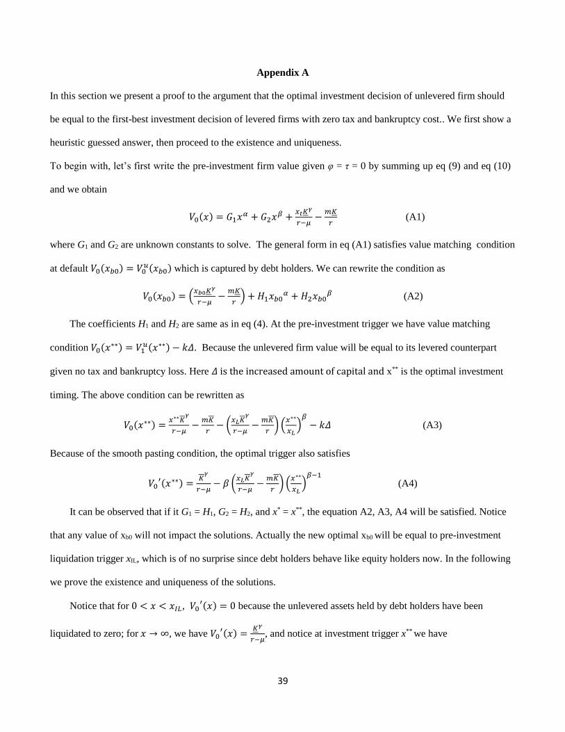
39
Appendix A
In this section we present a proof to the argument that the optimal investment decision of unlevered firm should
be equal to the first-best investment decision of levered firms with zero tax and bankruptcy cost.. We first show a
heuristic guessed answer, then proceed to the existence and uniqueness.
To begin with, let’s first write the pre-investment firm value given φ = τ = 0 by summing up eq (9) and eq (10)
and we obtain
𝑉0(𝑥) = 𝐺1𝑥𝛼 + 𝐺2𝑥𝛽 +𝑥𝑡𝐾𝛾
𝑟−𝜇−
𝑚𝐾
𝑟 (A1)
where G1 and G2 are unknown constants to solve. The general form in eq (A1) satisfies value matching condition
at default 𝑉0(𝑥𝑏0) = 𝑉0𝑢(𝑥𝑏0) which is captured by debt holders. We can rewrite the condition as
𝑉0(𝑥𝑏0) = (𝑥𝑏0𝐾𝛾
𝑟−𝜇−
𝑚𝐾
𝑟) + 𝐻1𝑥𝑏0
𝛼 + 𝐻2𝑥𝑏0𝛽 (A2)
The coefficients H1 and H2 are same as in eq (4). At the pre-investment trigger we have value matching
condition 𝑉0(𝑥∗∗) = 𝑉1𝑢(𝑥∗∗) − 𝑘𝛥. Because the unlevered firm value will be equal to its levered counterpart
given no tax and bankruptcy loss. Here 𝛥 is the increased amount of capital and x** is the optimal investment
timing. The above condition can be rewritten as
𝑉0(𝑥∗∗) =𝑥∗∗𝐾
𝛾
𝑟−𝜇−
𝑚𝐾
𝑟− (
𝑥𝐿𝐾𝛾
𝑟−𝜇−
𝑚𝐾
𝑟) (
𝑥∗∗
𝑥𝐿)
𝛽− 𝑘𝛥 (A3)
Because of the smooth pasting condition, the optimal trigger also satisfies
𝑉0′(𝑥∗∗) =
𝐾𝛾
𝑟−𝜇− 𝛽 (
𝑥𝐿𝐾𝛾
𝑟−𝜇−
𝑚𝐾
𝑟) (
𝑥∗∗
𝑥𝐿)
𝛽−1 (A4)
It can be observed that if it G1 = H1, G2 = H2, and x* = x**, the equation A2, A3, A4 will be satisfied. Notice
that any value of xb0 will not impact the solutions. Actually the new optimal xb0 will be equal to pre-investment
liquidation trigger xIL, which is of no surprise since debt holders behave like equity holders now. In the following
we prove the existence and uniqueness of the solutions.
Notice that for 0 < 𝑥 < 𝑥𝐼𝐿, 𝑉0′(𝑥) = 0 because the unlevered assets held by debt holders have been
liquidated to zero; for 𝑥 → ∞, we have 𝑉0′(𝑥) =
𝐾𝛾
𝑟−𝜇, and notice at investment trigger x** we have

40
𝑉0′(𝑥∗∗) =
𝐾𝛾
𝑟−𝜇− 𝛽 (
𝑥𝐿𝐾𝛾
𝑟−𝜇−
𝑚𝐾
𝑟) (
𝑥∗∗
𝑥𝐿)
𝛽−1<
𝐾𝛾
𝑟−𝜇 (A5)
To show this, we need to prove the second item is positive. Actually, it can be easily observed that 𝛽 (𝑥𝐿𝐾
𝛾
𝑟−𝜇−
𝑚𝐾
𝑟) =
𝛽
𝛽−1
𝑚𝐾
𝑟> 0. Thus there must have solutions for x** within (0 , ∞) . Recall the general solution (A1) is
governed by Hamilton-Jacoby-Bellman equation
𝑟𝑉0(𝑥) =1
2𝜎2𝑥2𝑉0
′′ + 𝑥𝑉0′ + 𝑥𝑡𝐾𝛾 − 𝑚𝐾 − 𝑐 (A6)
Now, suppose there are two solutions 𝑥1∗∗ < 𝑥2
∗∗ , which satisfy 𝑉0′(𝑥1
∗∗) = 𝑉0′(𝑥2
∗∗) = 𝛿 and 𝑉0′′(𝑥1
∗∗) < 0
and 𝑉0′′(𝑥2
∗∗) > 0, here δ denotes the slope level in eq(A5). Geometrically, we always can find at least one
intermediate 𝑥1∗∗ < 𝑥12
∗∗ < 𝑥2∗∗ such that 𝑉0
′(𝑥12∗∗) ≤ 𝛿 and 𝑉0
′′(𝑥12∗∗) = 0 and 𝑉0
′′′(𝑥12∗∗) > 0 due to the convex set.
To see the contradiction, let’s take first derivative of eq (A6) :
(𝑟 − 1)𝑉0′(𝑥) = (𝜎2 + 1)𝑥𝑉0
′′ +1
2𝜎2𝑥2𝑉0
′′′ + 𝐾𝛾 (A7)
However, 𝑥12∗∗ will not satisfy the eq (A7) because the left hand side is negative while the right hand side is
positive. The logic can be extended to multiple solutions assumption too. Our simple proof also can be applied to
solutions of second best investment policy, for which V0 will be replaced with E0.
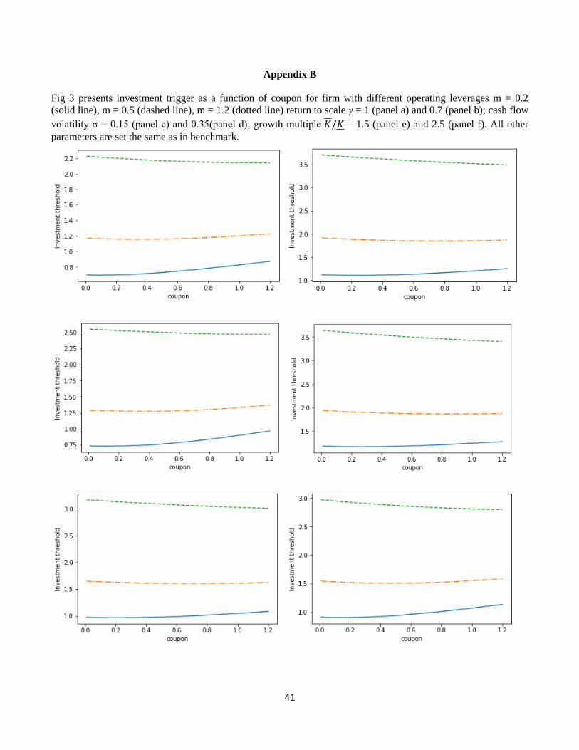
41
Appendix B
Fig 3 presents investment trigger as a function of coupon for firm with different operating leverages m = 0.2
(solid line), m = 0.5 (dashed line), m = 1.2 (dotted line) return to scale γ = 1 (panel a) and 0.7 (panel b); cash flow
volatility σ = 0.15 (panel c) and 0.35(panel d); growth multiple 𝐾/𝐾 = 1.5 (panel e) and 2.5 (panel f). All other
parameters are set the same as in benchmark.
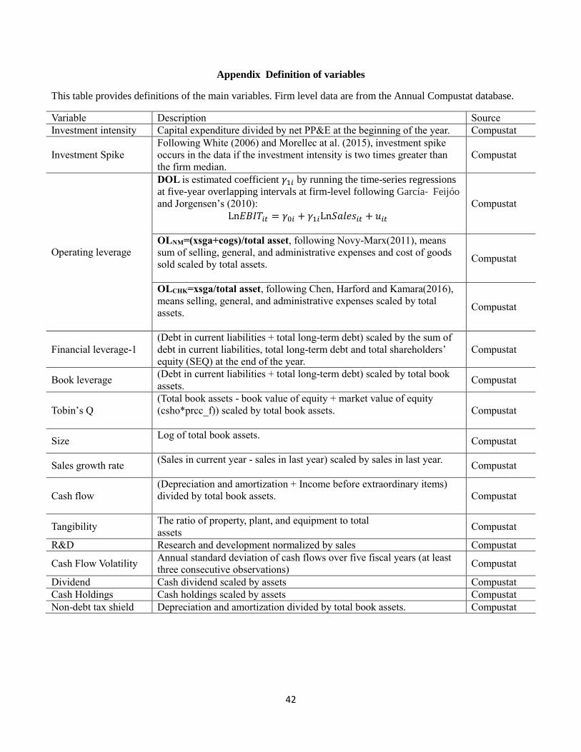
42
Appendix Definition of variables
This table provides definitions of the main variables. Firm level data are from the Annual Compustat database.
Variable Description Source
Investment intensity Capital expenditure divided by net PP&E at the beginning of the year. Compustat
Investment Spike
Following White (2006) and Morellec at al. (2015), investment spike
occurs in the data if the investment intensity is two times greater than
the firm median.
Compustat
Operating leverage
DOL is estimated coefficient 𝛾1𝑖 by running the time-series regressions
at five-year overlapping intervals at firm-level following García‐ Feijóo
and Jorgensen’s (2010):
Ln𝐸𝐵𝐼𝑇𝑖𝑡 = 𝛾0𝑖 + 𝛾1𝑖Ln𝑆𝑎𝑙𝑒𝑠𝑖𝑡 + 𝑢𝑖𝑡
Compustat
OLNM=(xsga+cogs)/total asset, following Novy-Marx(2011), means
sum of selling, general, and administrative expenses and cost of goods
sold scaled by total assets.
Compustat
OLCHK=xsga/total asset, following Chen, Harford and Kamara(2016),
means selling, general, and administrative expenses scaled by total
assets.
Compustat
Financial leverage-1
(Debt in current liabilities + total long-term debt) scaled by the sum of
debt in current liabilities, total long-term debt and total shareholders’
equity (SEQ) at the end of the year.
Compustat
Book leverage (Debt in current liabilities + total long-term debt) scaled by total book
assets. Compustat
Tobin’s Q
(Total book assets - book value of equity + market value of equity
(csho*prcc_f)) scaled by total book assets.
Compustat
Size Log of total book assets.
Compustat
Sales growth rate (Sales in current year - sales in last year) scaled by sales in last year.
Compustat
Cash flow
(Depreciation and amortization + Income before extraordinary items)
divided by total book assets.
Compustat
Tangibility The ratio of property, plant, and equipment to total
assets Compustat
R&D Research and development normalized by sales Compustat
Cash Flow Volatility Annual standard deviation of cash flows over five fiscal years (at least
three consecutive observations) Compustat
Dividend Cash dividend scaled by assets Compustat
Cash Holdings Cash holdings scaled by assets Compustat
Non-debt tax shield Depreciation and amortization divided by total book assets. Compustat