opportunistic scheduling, cooperative relaying and ... · chandrashekhar thejaswi pataguppe...
TRANSCRIPT

Opportunistic Scheduling, Cooperative Relaying and Multicast in Wireless Networks
by
Chandrashekhar Thejaswi Pataguppe Suryanarayan Bhat
A Dissertation Presented in Partial Ful�llmentof the Requirements for the Degree
Doctor of Philosophy
Approved February 2011 by theGraduate Supervisory Committee:
Junshan Zhang, ChairDouglas Cochran
Yu HuiThomas TaylorTolga Duman
ARIZONA STATE UNIVERSITY
May 2011

ABSTRACT
This dissertation builds a clear understanding of the role of information in wire-
less networks, and devises adaptive strategies to optimize the overall performance. The
meaning of information ranges from channel/network states to the structure of the signal
itself. Under the common thread of characterizing the role of information, this disserta-
tion investigates opportunistic scheduling, relaying and multicast in wireless networks.
To assess the role of channel state information, the problem of opportunistic
distributed opportunistic scheduling (DOS) with incomplete information is considered
for ad-hoc networks in which many links contend for the same channel using random
access. The objective is to maximize the system throughput. In practice, link state
information is noisy, and may result in throughput degradation. Therefore, re�ning the
state information by additional probing can improve the throughput, but at the cost of
further probing. Capitalizing on optimal stopping theory, the optimal scheduling policy
is shown to be threshold-based and is characterized by either one or two thresholds,
depending on network settings.
To understand the bene�ts of side information in cooperative relaying scenarios,
a basic model is explored for two-hop transmissions of two information �ows which
interfere with each other. While the �rst hop is a classical interference channel, the
second hop can be treated as an interference channel with transmitter side information.
Various cooperative relaying strategies are developed to enhance the achievable rate. In
another context, a simple sensor network is considered, where a sensor node acts as a
relay, and aids fusion center in detecting an event. Two relaying schemes are considered:
analog relaying and digital relaying. Su�cient conditions are provided for the optimality
of analog relaying over digital relaying in this network.
To illustrate the role of information about the signal structure in joint source-
channel coding, multicast of compressible signals over lossy channels is studied. The
focus is on the network outage from the perspective of signal distortion across all re-
ceivers. Based on extreme value theory, the network outage is characterized in terms
of key parameters. A new method using subblock network coding is devised, which
prioritizes resource allocation based on the signal information structure.
i

To Anna (my late father) and Pachanna (my late brother)
who instilled an unquenchable thirst for knowledge in me.
ii

ACKNOWLEDGEMENTS
I am greatly indebted to my advisor, Prof. Junshan Zhang, for his support
(�nancial, professional and moral) and his close guidance. I have always admired his
passion and enthusiasm towards research and formulating interesting problems. His
unquenchable thirst and excitement towards solving new problems and deriving useful
insights has always inspired me. Through several insightful discussions, he has taught
me a lot about what it takes to be a good researcher and a good writer. Moreover,
he is a very kind person and has been always accessible to discuss technical as well as
personal problems with him. He has been a great philosopher, friend and guide to me
during my stay as a PhD student. I am very fortunate to have him as my advisor.
Another individual who deeply in�uenced me is Prof. Cochran, with whom I
had the opportunity to work on a part of my research. I thank him for giving me an
opportunity to work with him and teaching me how to ask simple but fundamental
questions while doing research. I truly appreciate his patience and am very grateful to
him for all support and time he gave to me despite his busy schedule.
I thank Prof. Duman for teaching me the fundamentals of wireless communi-
cations, and space-time coding theory. Several technical discussions I had with him
were really valuable and helped me in strengthening my fundamentals, and in building
a strong foundation for my research. I would also like to thank Prof. Hui and Prof.
Taylor for serving my thesis committee and for their valuable suggestions to shape my
research.
Many thanks to my current and former colleagues: Dong, Weiyan, Qinghai,
Shanshan, Lei, Miao, Dajun, Sugumar, Tuan, Xiaowen, Brian and Eric for the pleasant
and inspiring discussions. I also thank my collaborators: Simon and Amir, for the
insightful discussions I had with them.
I am grateful to my wife Smitha for her patience, understanding, support and
for putting up with me during my PhD. I am grateful to my mother, sisters, broth-
ers, brothers-in-law and sisters-in-law for their constant encouragement and support
throughout my life. I also thank my father-in-law and mother-in-law for the excitement
and interest they showed in the progress of my research. It has been a great pleasure
iii

to interact, rag and mentor my nephews Manja, Pallu and my sister-in-law Priyanka.
It has been equally blissful to play with my cute nieces Manasa, Spoorthi, Shreya and
Raksha. I am really fortunate to have such a wonderful family.
Finally, I would also like thank all my teachers, friends and relatives without
whose support and encouragement, I could not have come this far.
iv

TABLE OF CONTENTS
Page
TABLE OF CONTENTS . . . . . . . . . . . . . . . . . . . . . . . . . . . . . . . v
LIST OF TABLES . . . . . . . . . . . . . . . . . . . . . . . . . . . . . . . . . . viii
LIST OF FIGURES . . . . . . . . . . . . . . . . . . . . . . . . . . . . . . . . . . ix
CHAPTER . . . . . . . . . . . . . . . . . . . . . . . . . . . . . . . . . . . . . . . 1
1 INTRODUCTION . . . . . . . . . . . . . . . . . . . . . . . . . . . . . . . . . 1
1.1 Distributed Opportunistic Scheduling . . . . . . . . . . . . . . . . . . . 3
1.2 Two-Hop Interference Flows . . . . . . . . . . . . . . . . . . . . . . . . 4
1.3 Multicast of Compressible Signals . . . . . . . . . . . . . . . . . . . . . . 6
1.4 Analog versus Digital Relaying in a Sensor Network . . . . . . . . . . . . 8
2 DISTRIBUTED OPPORTUNISTIC SCHEDULING WITH INCOMPLETE
STATE INFORMATION . . . . . . . . . . . . . . . . . . . . . . . . . . . . . 9
2.1 Introduction . . . . . . . . . . . . . . . . . . . . . . . . . . . . . . . . . . 9
2.2 Background and System Model . . . . . . . . . . . . . . . . . . . . . . . 12
Preliminaries on optimal stopping theory . . . . . . . . . . . . . . . . . . 12
System model . . . . . . . . . . . . . . . . . . . . . . . . . . . . . . . . . 13
DOS with one-level probing . . . . . . . . . . . . . . . . . . . . . . . . . 16
2.3 DOS with Two-Level Probing . . . . . . . . . . . . . . . . . . . . . . . . 19
Second-level probing . . . . . . . . . . . . . . . . . . . . . . . . . . . . . 19
Scheduling options and rewards . . . . . . . . . . . . . . . . . . . . . . . 21
Structure of optimal scheduling strategy . . . . . . . . . . . . . . . . . . 24
Optimality conditions . . . . . . . . . . . . . . . . . . . . . . . . . . . . 27
Numerical results . . . . . . . . . . . . . . . . . . . . . . . . . . . . . . . 27
2.4 DOS with Two-Level Probing: A Case with Limited Feedback . . . . . . 28
One-level probing . . . . . . . . . . . . . . . . . . . . . . . . . . . . . . . 28
Two-level probing . . . . . . . . . . . . . . . . . . . . . . . . . . . . . . . 29
2.5 Conclusion . . . . . . . . . . . . . . . . . . . . . . . . . . . . . . . . . . 32
3 TWO-HOP INTERFERENCE FLOWS: A CASE OF INTERFERENCE CHAN-
NELS WITH PARTIAL SIDE INFORMATION . . . . . . . . . . . . . . . . 34
v

Chapter Page3.1 Introduction . . . . . . . . . . . . . . . . . . . . . . . . . . . . . . . . . . 34
3.2 System Model and Background . . . . . . . . . . . . . . . . . . . . . . . 38
Transmission from sources: the �rst-hop communications . . . . . . . . . 40
Transmission from relays with partial side information: the second hop
communications . . . . . . . . . . . . . . . . . . . . . . . . . . . 41
3.3 Layered Coding for Second-Hop Communications: IC with Partial Side-
Information . . . . . . . . . . . . . . . . . . . . . . . . . . . . . . . . . . 42
Layered binning for interference cancelation . . . . . . . . . . . . . . . . 42
Superposition coding for interference cancelation . . . . . . . . . . . . . 45
3.4 The Gaussian Case with Symmetric Channel Gains . . . . . . . . . . . 49
Binning for interference cancelation: layered dirty paper coding (DPC) . 50
Superposition coding: layered beamforming . . . . . . . . . . . . . . . . 55
3.5 Numerical Examples . . . . . . . . . . . . . . . . . . . . . . . . . . . . . 59
3.6 Conclusions . . . . . . . . . . . . . . . . . . . . . . . . . . . . . . . . . . 60
4 WHEN COMPRESSIVE SAMPLINGMEETSMULTICAST: OUTAGE ANAL-
YSIS AND SUBBLOCK NETWORK CODING . . . . . . . . . . . . . . . . 62
4.1 Introduction . . . . . . . . . . . . . . . . . . . . . . . . . . . . . . . . . . 62
4.2 System Model and Background . . . . . . . . . . . . . . . . . . . . . . . 67
4.3 Transmission Strategies: Outage Analysis . . . . . . . . . . . . . . . . . 69
Transmission of compressed measurements (TCM) . . . . . . . . . . . . 69
Transmission of coe�cients (TC) . . . . . . . . . . . . . . . . . . . . . . 72
4.4 Network Coding for Power-law Decay Signals . . . . . . . . . . . . . . . 74
Traditional network coding for power-law decay signals . . . . . . . . . . 74
Subblock network coding for power-law decay signals . . . . . . . . . . . 76
Two-step heuristic greedy algorithm . . . . . . . . . . . . . . . . . . . . 77
4.5 Numerical Example and Discussions . . . . . . . . . . . . . . . . . . . . 79
Basic setup . . . . . . . . . . . . . . . . . . . . . . . . . . . . . . . . . . 79
Numerical results . . . . . . . . . . . . . . . . . . . . . . . . . . . . . . . 81
4.6 Conclusions . . . . . . . . . . . . . . . . . . . . . . . . . . . . . . . . . . 82
vi

Chapter Page5 DIGITAL RELAYING VERSUS ANALOG RELAYING: A SUFFICIENT
CONDITION FOR OPTIMALITY . . . . . . . . . . . . . . . . . . . . . . . 84
5.1 Introduction . . . . . . . . . . . . . . . . . . . . . . . . . . . . . . . . . . 84
5.2 System Model . . . . . . . . . . . . . . . . . . . . . . . . . . . . . . . . . 86
5.3 Relaying Schemes . . . . . . . . . . . . . . . . . . . . . . . . . . . . . . . 88
Digital relaying (detect and forward) . . . . . . . . . . . . . . . . . . . . 88
Analog relaying (estimate and forward) . . . . . . . . . . . . . . . . . . . 91
5.4 Comparison of Analog and Digital Relaying . . . . . . . . . . . . . . . . 92
5.5 Simulation Results . . . . . . . . . . . . . . . . . . . . . . . . . . . . . . 93
5.6 Conclusions . . . . . . . . . . . . . . . . . . . . . . . . . . . . . . . . . . 94
6 CONCLUSIONS AND DISCUSSIONS . . . . . . . . . . . . . . . . . . . . . 95
6.1 Distributed Opportunistic Scheduling . . . . . . . . . . . . . . . . . . . . 95
6.2 Cooperative Relaying . . . . . . . . . . . . . . . . . . . . . . . . . . . . . 97
6.3 Digital versus Analog Relaying . . . . . . . . . . . . . . . . . . . . . . . 98
6.4 Multicasting . . . . . . . . . . . . . . . . . . . . . . . . . . . . . . . . . . 99
REFERENCES . . . . . . . . . . . . . . . . . . . . . . . . . . . . . . . . . . . . 100
APPENDIX . . . . . . . . . . . . . . . . . . . . . . . . . . . . . . . . . . . . . . 110
A PROOFS OF RESULTS FROM CHAPTER 2 . . . . . . . . . . . . . . . . . 111
A.1 Derivation of Rate Equation (2.11) . . . . . . . . . . . . . . . . . . . . . 111
A.2 Proof of Lemma 2.1 . . . . . . . . . . . . . . . . . . . . . . . . . . . . . 112
A.3 Proof of Lemma 2.2 . . . . . . . . . . . . . . . . . . . . . . . . . . . . . 113
A.4 Proof of Theorem 2.1 . . . . . . . . . . . . . . . . . . . . . . . . . . . . . 114
A.5 Proof of Theorem 2.2 . . . . . . . . . . . . . . . . . . . . . . . . . . . . . 115
A.6 Proof of Lemma 2.5 . . . . . . . . . . . . . . . . . . . . . . . . . . . . . 116
B PROOFS OF RESULTS FROM CHAPTER 3 . . . . . . . . . . . . . . . . . 119
B.1 Proof of Theorem 3.1 . . . . . . . . . . . . . . . . . . . . . . . . . . . . . 119
B.2 Proof of Theorem 3.2 . . . . . . . . . . . . . . . . . . . . . . . . . . . . . 123
B.3 Proof of Proposition 3.1 . . . . . . . . . . . . . . . . . . . . . . . . . . . 126
B.4 Determining DPC matrices and derivations of (3.11) and (3.12) . . . . . 128
vii

LIST OF TABLES
Table Page
B.1 Table depicting the error events (i = ∗ if i = 1) . . . . . . . . . . . . . . . . 122
B.2 Table depicting the error events (i = ∗ if i = 1) . . . . . . . . . . . . . . . . 125
viii

LIST OF FIGURES
Figure Page
2.1 A sample realization of channel probing and data transmission. . . . . . . . 14
2.2 A sketch of DOS with two-level probing. . . . . . . . . . . . . . . . . . . . . 19
2.3 A structural sketch for Strategy A. . . . . . . . . . . . . . . . . . . . . . . . 25
2.4 A structural sketch for Strategy B. . . . . . . . . . . . . . . . . . . . . . . . 25
2.5 Relative gain Γ as a function of α = ρM . . . . . . . . . . . . . . . . . . . . 28
3.1 A sketch of two-hop interference �ows. . . . . . . . . . . . . . . . . . . . . . 39
3.2 ILD vs. Rc curves (α = 0.2). . . . . . . . . . . . . . . . . . . . . . . . . . . . 59
3.3 ILD vs. Rc curves (α = 0.6). . . . . . . . . . . . . . . . . . . . . . . . . . . . 59
4.1 Multicast transmission of compressible data (a) conventional method; (b)
transmission of compressed measurements (c) proposed joint compressive
sensing and network coding. . . . . . . . . . . . . . . . . . . . . . . . . . . . 66
4.2 P ∗out vs. ϵ. . . . . . . . . . . . . . . . . . . . . . . . . . . . . . . . . . . . . . 82
4.3 Normalized Avg. MSE vs. ϵ. . . . . . . . . . . . . . . . . . . . . . . . . . . . 82
5.1 Block diagram of a typical sensor relay network. . . . . . . . . . . . . . . . 86
5.2 Pe vs. SNRl for SNRo = 3 dB. . . . . . . . . . . . . . . . . . . . . . . . . . . . 94
5.3 Pe vs. SNRl for SNRo = −3 dB. . . . . . . . . . . . . . . . . . . . . . . . . . . 94
ix

Chapter 1
INTRODUCTION
Recent years have witnessed a tremendous growth in the demand for ubiquitous infor-
mation access. Indeed, our society hinges heavily on reliable and e�cient operations
of large-scale networks, e.g., the Internet and wireless ad-hoc/sensor networks, for col-
lecting, processing, analyzing and managing information in adverse noisy environments.
The unique characteristics of wireless links, together with the bursty nature of tra�c
�ows, create both new challenges and opportunities in our attempts to implement this
vision. Di�erent from the wireline counterpart, the design of wireless networks faces a
number of unique challenges, particularly, co-channel interference and multipath fading.
1) Co-channel interference: When more than one information �ow occupies the same
channel, the shared nature of wireless medium results in co-channel interference. The
receiver, apart form the message of its own source, also receives transmissions from
other unintended sources. This may lead to collisions and transmission outages. Wire-
less systems deal with interference by incorporating time/frequency orthogonality, or by
handling at the medium access control (MAC)-layer level, typically, via scheduling or
random access protocols.
2) Time varying channel conditions over fading channels: Fading is the time variation
of the wireless channel, and can often be characterized with two types of e�ects: large-
scale path loss and shadowing e�ects that cause the signal to attenuate with distance;
and multipath scattering e�ects that result in delayed copies of the signal adding up
constructively or destructively at the receiver. Fading e�ects are often mitigated at the
physical layer using coding/modulation and diversity techniques.
Besides the above impediments, wireless networks often operate under hostile
conditions that include bursty tra�c and changing network topology. Meeting the qual-
ity of services (QoS) requirements of the end users can be extremely di�cult in such
hostile operating conditions.
Further, for practical reasons, wireless systems are often constrained in terms
of resources such as bandwidth, power, time etc. The impetus for the optimal design
and operation of any wireless system lies in the e�cient management of these limited
1

resources. E�ective management of limited resources, in turn, hinges heavily on the
availability of information about the system states in the presence of complicated dy-
namics in the network. For instance, in multimedia systems, availability of a priori
information about the parameters, such as the distribution and �compressibility� of the
signals, helps in e�cient data compression, thereby saving storage and transmission
bandwidth. In multiuser wireless networks, the availability of information about the dy-
namics of the channel state, tra�c �ow, topology etc., at each epoch, can be leveraged
using the notion of opportunistic scheduling to signi�cantly enhance the QoS provision-
ing. Also, in networks where interference is the main impediment, access to information
about the interference and its structure enables e�cient design of transmission/reception
techniques toward optimal interference management.
Thus motivated, one primary goal of this work is to understand the �value of
information� in enhancing the system performance. As noted above, the meaning of
information ranges from state information about the channel/network dynamics to the
structure of the source signal itself. By developing a clear understanding of various forms
of information availability, we demonstrate that indeed one can gain substantially, in
terms of overall performance, when compared to the methods which do not exploit the
availability of information.
Under the common theme of characterizing the value of information, this thesis is
broadly organized into four chapters. In Chapter 2, distributed opportunistic scheduling
(DOS) is studied with the objective of quantifying the trade-o� between throughput
gain with re�ned channel state information and the corresponding overhead. Based
on optimal stopping theory, a framework for PHY-aware scheduling is developed for
exploiting rich diversities at the physical-layer and medium access control (MAC) layer.
In Chapter 3, a two-hop interference network is studied, in which the second hop is
viewed as an interference channel with side information at the transmitters. Information
theoretic techniques are applied to study the value of this side information in enhancing
the achievable rate. In Chapter 4, the problem of multicasting compressible signals is
considered, where one principal objective is to exploit the information available on the
signal structure in developing joint source/channel coding strategy to improve the QoS.
2

In Chapter 5, a sensory relay network model is considered, and optimality conditions
for analog vs digital relaying are characterized. In what follows, we brie�y summarize
our contributions along with the motivations and techniques involved.
1.1 Distributed Opportunistic Scheduling
As noted above, two key challenges to the wireless communications are interference and
fading. In the design of wireless ad-hoc networks, the traditional approach has been
to separate packet losses caused by fading from those caused by collision, neglecting
the structure pertaining to the dynamics of these parameters in the networks. That
is, the PHY layer addresses the issues of fading, and the MAC layer addresses the
issue of contention. However, as shown in [1, 2], fading can often adversely a�ect the
MAC layer in many realistic scenarios. The coupling between the temporal dynamics of
fading and MAC calls for a uni�ed PHY/MAC design for wireless ad-hoc networks in
order to achieve optimal throughput and latency. Indeed, lurking beneath this dynamic
nature of the wireless medium and tra�c are the joint PHY/MAC diversities (including
multiuser, time and spatial diversities), which are available for exploitation in a wide
range of wireless scenarios. Nevertheless, one has to carefully understand these dynamics
and build channel-aware scheduling approaches for e�cient handling of the information
�ow. It is therefore of critical importance to develop a rigorous understanding of state-
aware scheduling that can resolve contention and mitigate interference e�ciently while
exploiting diversities.
Notably, there has recently been a surge of interest in channel-aware scheduling
and channel-aware access control. Channel-aware opportunistic scheduling was �rst de-
veloped for downlink transmissions in multiuser wireless networks ([3],[4],[5],[6]). While
these studies assumed centralized scheduling, distributed opportunistic scheduling was
initiated by Zheng et al. [7], where, using optimal stopping theory, authors devise
scheduling strategies for ad-hoc networks under the assumption that the nodes have
perfect channel information. Generalization of [7] to the noisy estimation case is carried
out in [8]. It has been observed in [9] that the errors in channel estimation results in
outages, and they propose backo� schemes to avoid transmission outages. However,
3

backo� may lead to severe throughput degradation, especially in the low SNR regime,
due to a more conservative rate reduction. Therefore, a plausible solution is to mitigate
rate estimation errors by performing further channel probing. Clearly, the improved rate
estimation obtained with second-level probing enables the desired link to make more ac-
curate decisions. However, the advantages of second-level probing come at the price of
additional overhead. There is, therefore, a tradeo� between the throughput gain from
better channel conditions and the cost for further probing.
With this insight, in Chapter 2, we investigate DOS with two-level channel prob-
ing by optimizing the tradeo� between the throughput gain from more accurate rate es-
timation and the resulting additional probing overhead. Based on the recent advances in
OST, namely OST with two-level incomplete information [10] and statistical versions of
�prophet inequalities� [11], we show that the optimal scheduling policy is threshold-based
and is characterized by either one or two thresholds, depending on network settings. Nec-
essary and su�cient conditions for both cases are rigorously established. In particular,
our analysis reveals that performing second-level channel probing is optimal when the
�rst-level estimated channel condition falls in between the two thresholds. Numerical
results are provided to illustrate the e�ectiveness of the proposed DOS with two-level
channel probing. We also extend our study to the case with limited feedback, where the
feedback from the receiver to its transmitter takes the form of (0, 1, e).
1.2 Two-Hop Interference Flows
Relay channels and interference channels have been basic building blocks of wireless net-
works. Particularly, interference in networks is modeled by a basic two user interference
channel (IC), which consists of two transmitter-receiver pairs involved in simultaneous
communication, and their transmissions interfere with each other. As noted earlier, in-
terference is a central phenomenon in wireless communications. Most state-of-the-art
wireless systems deal with interference in one of two ways: orthogonalize the commu-
nication links in time or frequency, so that they do not interfere with each other; or,
allow the communication links to share the same degrees of freedom, but treat each
other's interference as adding to the noise �oor. It is clear that both approaches can be
4

sub-optimal. The �rst approach entails an a priori loss of degrees of freedom in both
links, no matter how weak the potential interference is. The second approach treats
interference as pure noise while it actually carries information and has structure that
can potentially be exploited in mitigating its e�ect.
Unfortunately, the problem of characterizing the capacity region of a general
IC has been open. The only case in which the capacity is known is in the strong
interference case, where each receiver has a better reception of the other user's signal
than the intended receiver [12]. The best known strategy for the general case is due to
Han and Kobayashi (HK) [13]. This strategy is a natural one and involves splitting the
transmitted information of both users into two parts: private information to be decoded
only at its own receiver and common information that can be decoded at both receivers.
By decoding the common information, part of the interference can be canceled o�, while
the remaining private information from the other user is treated as noise. Recently,
Etkin and Tse [14], have proposed a speci�c HK type scheme where it is shown that the
proposed scheme achieves to within a single bit of the capacity region of an IC.
In a relay channel, as introduced by van der Meulen [15], a relay node assists
the source in communicating data to a destination. Relay networks are instrumental in
harnessing the dynamic nature of the wireless medium to yield a form of diversity called
cooperative diversity [16].
An interesting model under consideration can be viewed as a combination of
relay channels and interference channels. Speci�cally, this model involves two sources
which communicate simultaneously with two destinations, and are aided by two relay
nodes. While the �rst hop is akin to the traditional interference channel, the second
hop has an interesting feature. Speci�cally, as a by-product of the Han-Kobayashi [13]
transmission scheme applied to the �rst hop, each of the relays (in the second hop) has
access to some of the data that is intended to the other destination, in addition to its
own data. Thus, the second hop represents an interference channel with side information
at the transmitters. This feature opens the door to cooperation between the relays. A
clear understanding towards exploiting side information at the relays in the second hop
enables one to devise relaying strategies to manage interference and e�cient information
5

�ow, thereby enhancing the achievable rate region of the network.
In Chapter 3, we explore some cooperative strategies among relays that system-
atically exploit the availability of side information to maximize the achievable rates.
Speci�cally, we observe that the availability of side information at each relay opens the
door for cooperation which can take the form of distributed multiple-input and multiple-
output (MIMO) broadcast, thus greatly enhancing its e�ectiveness at high SNR. How-
ever, since each relay has only partial side information of the data beyond its own, full
cooperation is not possible. Thus, a key feature of this network is that it has elements
of both the broadcast channel and the interference channel.
In light of this, we study strategies based on the nontrivial marriage of MIMO-BC
techniques for cooperative relaying, rate-splitting and superposition coding, to enable
interference cancelation at the receivers, and the Gelfand-Pinsker (GP) coding [17] at
each transmitter to reduce the interference to its own receivers. Speci�cally, we propose
two types of layered schemes that combine MIMO broadcast and HK coding. The �rst
one is layered coding with binning which mainly hinges on a novel interplay between
binning (DPC) and HK coding. The second one is a layered coding with superposition
strategy that involves superposition coding over di�erent tiers. Numerical results are
provided that indicate our approaches provide substantial bene�ts at high SNR.
1.3 Multicast of Compressible Signals
Reliable delivery of compressible information to many destinations is an important sce-
nario in modern day wireless systems. This transmission scenario, for instance, is useful
for multimedia streaming over a WiFi or WiMAX network with multiple receivers. It
is also applicable to sensor networks, where each sensor node wishes to communicate
its sensed observations to multiple coordinating agents. Needless to say, this problem
is quite challenging due to the lossy nature of wireless channels and the heterogeneity
in the amount of information received across di�erent receivers. Another challenge is
the �bottleneck� e�ect with the shared transmission medium among many receivers; i.e.,
the overall performance is limited by the receiver that has the worst channel condition.
Therefore, ensuring that the QoS for the bottleneck user is on par with the others clearly
6

makes the multicast transmission more challenging. In light of this, it is of paramount
importance to come up with transmission schemes that can mitigate channel erasures so
that data loss is minimized. Notably, network coding (NC), a recent breakthrough in this
avenue by Ahlswede et al. [18], o�ers a promising platform for multicast transmissions.
When we consider source signals for transmission, many of these signals are
known to be sparse or compressible. The conventional method of data compression
involves sampling the signal at the Nyquist's rate, storing the samples, and compressing
them in an appropriate domain prior to the transmission, which would incur heavy
sampling and storing burden at the sender. On the other hand, recent developments of
compressive sensing theory [19, 20, 21] have provided methods not only for lower-rate
signal acquisition, but also for accurate signal reconstruction.
When it comes to transmission of compressible data over wireless links, the
traditional wisdom has been to adopt separation principle. That is, while the structure
of the source signal is considerably exploited in sampling and compression, it is seldom
exploited in minimizing the �information loss� incurred due to transmission over the
hostile channel. This calls for joint design of compression and transmission strategies to
enhance the �ow of information.
With this motivation, in Chapter 4, we study multicasting compressively sampled
signals from a source to many receivers, over lossy wireless channels. Our focus is on
the network outage from the perspective of signal distortion across all receivers, for
both cases where the transmitter may or may not be capable of reconstructing the
compressively sampled signals. Capitalizing on extreme value theory, we characterize
the network outage in terms of key system parameters, including the erasure probability,
the number of receivers and the sparse structure of the signal. We show that when
the transmitter can reconstruct the compressively sensed signal, the strategy of using
network coding to multicast the reconstructed signal coe�cients can reduce the network
outage signi�cantly. We observe, however, that the traditional network coding could
result in suboptimal performance for power-law decay signals. Thus motivated, we
devise a new method, namely subblock network coding, that exploits the knowledge
about the signal structure. Essentially, subblock coding involves fragmenting the data
7

into subblocks, and allocating time slots to di�erent subblocks, based on their priorities.
We formulate the corresponding optimal allocation as an integer programming problem.
Since integer programming is often intractable, we develop a heuristic algorithm that
prioritizes the time slot allocation by exploiting the inherent priority structure of power-
law decay signals. Numerical results show that the proposed schemes outperform the
traditional methods with signi�cant margins.
1.4 Analog versus Digital Relaying in a Sensor Network
In Chapter 5, we consider a simple model of wireless sensor network for hypothesis
testing, where a sensor node acts as a relay and aids a fusion center to perform hypothesis
testing on an event. The sensor performs noisy observations on the underlying event,
performs a local processing and then relays the processed data to the fusion center.
We compare two relay schemes: �estimate-and-forward� (analog relaying) and �detect-
and-forward� (digital relaying), in terms of the ultimate detection performance they
support at the fusion center. With this performance criterion, the relative merit of the
two schemes is shown to depend on the observation SNR at the sensor and the SNR
of the communication link connecting the sensor and the fusion center. A su�cient
condition, in terms of these SNRs, for the superiority of digital relaying over analog
relaying is derived for this simple network model. Although the network model used
here is highly simpli�ed, it is hoped that this work will contribute to a foundation for
analysis of more realistic scenarios, leading to advances in sensor placement strategies
and inference algorithms in sensor networks. This study can also impact the development
of cooperative relaying strategies in wireless relay networks.
8

Chapter 2
DISTRIBUTED OPPORTUNISTIC SCHEDULING WITH INCOMPLETE STATE
INFORMATION
2.1 Introduction
Channel-aware scheduling has recently emerged as a promising technique to harness
the rich diversities inherent in wireless networks. In channel-aware scheduling, joint
physical layer (PHY)/medium access control (MAC) optimization is utilized to improve
network throughput by scheduling links with good channel conditions for data trans-
missions [3, 22, 6]. While most existing studies focus on centralized scheduling (see,
e.g., [4, 23, 24, 22, 6]), some initial steps have been taken in [25] to develop distributed
opportunistic scheduling (DOS) to reap multiuser diversity and time diversity in wireless
ad-hoc networks.
The DOS framework considers an ad-hoc network in which many links contend
for the same channel using random access, e.g., carrier-sense multiple-access (CSMA).
However, random access protocols provide no guarantee that a successful channel con-
tention is necessarily attained by a link with good channel conditions. From a holistic
perspective, a successful link with poor channel conditions should forgo its data trans-
mission and let all links re-contend for the channel. This is because after further channel
probing, it is more likely for a link with better channel conditions to take the channel,
yielding possibly higher throughput. In this way, multiuser diversity across links and
time diversity across time can be exploited in a joint manner. However, each channel
probing incurs a cost of contention time. The desired tradeo� between the through-
put gain from better channel conditions and the cost for further probing reduces to
judiciously choosing an optimal rule for stopping channel probing for throughput max-
imization. Using optimal stopping theory (OST), it is shown in [25] that the optimal
scheduling scheme turns out to be a pure threshold policy: The successful link proceeds
to transmit data only if its supportable rate is higher than the pre-designed threshold;
otherwise, it skips the transmission opportunity and lets all other links re-contend. In
general, threshold-based scheduling uses local information only, and hence is amenable
to easy distributed implementation in practical systems.
9

The initial study of DOS [25] hinges upon a key assumption that the channel
state information (CSI) is perfectly available at the receiver. In practice, the link rates
are estimated from noisy observations. It is shown in [9] that the signal-to-noise ratio
(SNR) estimated by the minimum mean squared error (MMSE) method is larger than
the �actual SNR� due to the estimation error noise. Thus, the transmission rate must be
backed o� from the estimated rate in order to avoid transmission outages. Our initial
steps in [8] show that the optimal scheduling policy under noisy channel estimation still
has a threshold structure.
Despite their robust performance under noisy channel estimation, the linear
backo� schemes proposed in [8] are reactive in nature and back o� the rate by a fac-
tor proportional to the channel estimation errors, which may lead to severe throughput
degradation, especially in the low SNR regime (where a more conservative rate backo�
is needed). Recently, wideband communications (e.g., ultra-wideband) has attracted
signi�cant attention [26], owing to its low-power operation and the ability to co-exist
with other legacy networks, etc. The great potential of wideband communications gives
an impetus to address the problem of throughput degradation due to estimation errors,
in the low-SNR (wideband) regime. More speci�cally, to circumvent this drawback, a
plausible solution is to mitigate the rate estimation errors by performing further chan-
nel probing. In the sequel, we refer to the initial rate estimation performed during the
channel contention as ��rst-level probing�, whereas the subsequent probing performed
after the successful contention is referred to as �second-level probing�. Clearly, the im-
proved rate estimation obtained with second-level probing enables the desired link to
make more accurate decisions. However, the advantages of second-level probing come
at the price of additional delay. This gives rise to two important questions: 1) Is it
worthwhile for the link with successful contention to perform further channel probing
to re�ne the rate estimate, at the cost of additional probing? 2) While there is always
a gain in the transmission rate due to the re�nement, how much can one bargain with
the additional probing overhead?
We shall answer these questions by considering distributed opportunistic schedul-
ing with two-level channel probing. Based on two recent advances in optimal stopping
10

theory, namely optimal stopping with two-level incomplete information [10] and statis-
tical versions of �prophet inequalities� [11], we provide a rigorous characterization of the
scheduling strategy that optimizes the tradeo� between the throughput gain achieved
by second-level channel probing and the resulting additional delay. It is shown that
the optimal scheduling strategy is threshold-based and is characterized by either one or
two thresholds, depending on the system parameters. By establishing the corresponding
necessary and su�cient conditions for these two cases, we show that the second-level
probing can signi�cantly improve the system throughput when the estimated rate via
�rst-level probing falls in between the two thresholds. In such scenarios, the cost of addi-
tional delay can be well justi�ed by the throughput enhancement using the second-level
channel probing. We elaborate further on this in Section 2.3. Finally, through numerical
results, we illustrate the e�ectiveness of the proposed scheduling scheme.
Before proceeding further, the main contributions distinguishing this work from
other existing works should be emphasized. OST under two levels of incomplete infor-
mation is addressed with the objective of maximizing the net-return in [10]; in contrast,
we study OST with two levels of probing as applied to DOS with the objective of max-
imizing the rate of return (i.e., the throughput). We study distributed opportunistic
scheduling for ad-hoc communications under noisy conditions where the rate estimate is
available only after a successful channel contention; and this is clearly di�erent from [9],
which considers centralized scheduling assuming that the rate estimates of all links are
available a priori at the base station. Despite the fact that both this work and [8] study
distributed opportunistic scheduling with imperfect information, this work concentrates
on proactively improving throughput by enhancing rate estimation, whereas [8] proposes
to passively reduce data rate to avoid transmission outages. Another related work [27]
uses optimal stopping theory to investigate the intrinsic trade-o� between energy and
delay in distributed data aggregation and forwarding in sensor networks.
The rest of the chapter is organized as follows. In Section 2.2, we provide a brief
introduction to the optimal stopping theory, discuss the system model, and provide
background on DOS with only �rst-level probing in noisy environments. In Section 2.3,
we present second-level channel probing and characterize the optimal DOS with two-
11

level probing. We also present numerical results to illustrate the gain due to two-level
probing. In Section 2.4, we extend our study to the case where there is limited feedback
from the receiver to its transmitter. Finally, Section 2.5 contains our conclusions.
Notation: |·| denotes the amplitude of the enclosed complex-valued quantity. R+
denotes the set of non-negative real numbers. We use [x]+ for max[x, 0], and E[·] for
expectation.
2.2 Background and System Model
Preliminaries on optimal stopping theory
As noted above, in an ad-hoc communication network with many links, when a link
discovers that its channel condition is �relatively poor� after a successful channel con-
tention, it can either transmit or skip this opportunity so that, in the next round, some
link with a better condition would have the chance to transmit. This is intimately re-
lated to the optimal stopping problem in sequential analysis [28]. Simply put, optimal
stopping theory is concerned with the problem of choosing a strategy for deciding when
to take a given action based on the past events in order to maximize an average return,
where return is the net gain (the di�erence between the reward and the cost). The
corresponding strategy is called an optimal stopping rule.
More speci�cally, let Z1, Z2, ... denote a sequence of random variables, and let
Y0, Y1(Z1), Y2(Z1, Z2), . . . , Y∞(Z1, Z2, . . .) a sequence of real-valued reward functions. The
reward is Yn(Z1, ..., Zn) if the strategy chooses to stop at time n. The theory of optimal
stopping is concerned with determining the stopping time N to maximize the expected
reward E[YN ]; and in general, a stopping rule (or a stopping time) (cf. [28]) is de�ned to
be a random variable N such that {N = n} ∈ Fn, where Fn is the σ-algebra generated
by {Z1, . . . , Zn}. This is equivalent to saying that the decision to transmit at a slot n
depends only on the sequence {Z1, . . . , Zn}. A good introduction to optimal stopping
theory can be found in [28],[29], or [30].
12

System model
Consider a single-hop ad-hoc network in which L links contend for the channel using
random access. A collision model is assumed for random access, in which a channel
contention of a link is said to be successful if no other links transmit at the same time.
Let pℓ be the probability that link ℓ contends for the channel, ℓ = 1, . . . , L. Then
the overall successful contention probability, ps, is given by ps =∑L
ℓ=1
(pℓ∏
i=ℓ(1− pi))
(cf. [31]). For ease of exposition, we assume that the contention probabilities, {pℓ},
remain �xed (see [32] for a study with adaptive contention probabilities). We de�ne the
random duration of achieving one successful channel contention as one round of channel
probing. Clearly, the number of slots in each probing round, K, is a geometric random
variable, i.e., K ∼ G(ps). Denoting the slot duration by τ , the corresponding random
duration for one probing round thus becomes Kτ , with its expected value being τ/ps.
In a nutshell, each round of channel probing consists of two phases, namely,
channel contention and channel estimation. We assume that a link can estimate its link
conditions (hence the transmission rate) after a successful contention1.
Let s(n) denote the successful link in the n-th round of channel probing, and Rn
denote the corresponding transmission rate. Due to the time-varying nature of wireless
channels, Rn is random. Following the standard assumption on block fading channels
in wireless communications [33], we assume that the channel remains constant for a
duration of T . When an estimate of the transmission rate is available, the successful
link may decide to transmit over a duration of T , if the rate is high enough, or may skip
it2 and allow all links to re-contend, in the hope that another link with a better channel
will take the channel later.
To get a more concrete sense of joint channel probing and distributed scheduling,
we depict, in Fig. 2.1, an example with N rounds of channel probing and one single
data transmission. Speci�cally, suppose after the �rst round of channel probing with a
duration of K1 slots, the rate, R1, of link s(1) is very small (indicating a poor channel
1The successful link can carry out its rate estimation via a training phase during the request-to-send/clear-to-send (RTS/CTS) handshake, which follows a successful contention. This procedure isfairly standard in the literature, and is not dealt with here.
2This decision can be broadcast to all users in the one-hop neighborhood (e.g., NCTS).
13
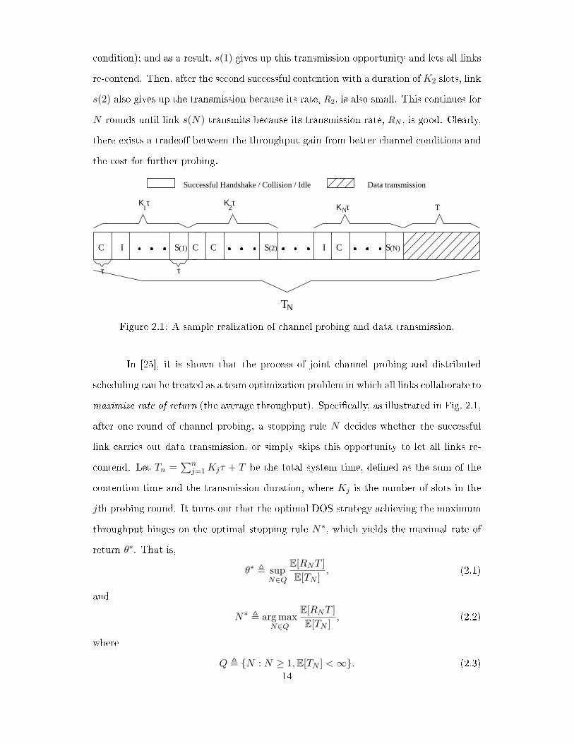
condition); and as a result, s(1) gives up this transmission opportunity and lets all links
re-contend. Then, after the second successful contention with a duration ofK2 slots, link
s(2) also gives up the transmission because its rate, R2, is also small. This continues for
N rounds until link s(N) transmits because its transmission rate, RN , is good. Clearly,
there exists a tradeo� between the throughput gain from better channel conditions and
the cost for further probing.
ττ
TN
N
(2) I CSC I (1)S C C (N)S
TΚ τ Κ τΚ τ21
Successful Handshake / Collision / Idle Data transmission
Figure 2.1: A sample realization of channel probing and data transmission.
In [25], it is shown that the process of joint channel probing and distributed
scheduling can be treated as a team optimization problem in which all links collaborate to
maximize rate of return (the average throughput). Speci�cally, as illustrated in Fig. 2.1,
after one round of channel probing, a stopping rule N decides whether the successful
link carries out data transmission, or simply skips this opportunity to let all links re-
contend. Let Tn =∑n
j=1Kjτ + T be the total system time, de�ned as the sum of the
contention time and the transmission duration, where Kj is the number of slots in the
jth probing round. It turns out that the optimal DOS strategy achieving the maximum
throughput hinges on the optimal stopping rule N∗, which yields the maximal rate of
return θ∗. That is,
θ∗ , supN∈Q
E[RNT ]
E[TN ], (2.1)
and
N∗ , argmaxN∈Q
E[RNT ]
E[TN ], (2.2)
where
Q , {N : N ≥ 1,E[TN ] <∞}. (2.3)14

It is clear that Rn plays a critical role in distributed opportunistic scheduling. In
practice, rate estimates are seldom perfect. It is shown in [9] that the rate corresponding
to the estimated SNR tends to be greater than the actual rate, and subsequently the
transmission rate must be backed o� from the estimated rate to avoid outages. Then,
a natural question to ask is whether it is worthwhile for the link with successful con-
tention to perform further channel probing to re�ne the channel estimate, at the cost of
additional probing overhead, and how much can one bargain?
Intuitively speaking, when the transmission rate is small, it makes sense to give
up the transmission, since the gain due to rate re�nement would be marginal due to the
poor link conditions. On the other hand, when the rate is large enough, it may not be
advantageous to perform additional probing as the improvement is meager. It is natural
to expect that there exists a �gray area� between these extremes where signi�cant gains
are possible by re�ning the rate estimate with additional probing. In what follows, we
seek a clear understanding of the above fundamental issues.
To this end, we present the PHY-layer signal model �rst. The received signal
corresponding to s(n) can be written as3
Ys(n)(n) =√ρhs(n)(n)Xs(n)(n) + ξs(n)(n), (2.4)
where ρ is the normalized receiver SNR, hs(n)(n) is the channel gain for link s(n),
Xs(n)(n) is the transmitted signal with E[∣∣Xs(n)(n)
∣∣2] = 1, and ξs(n)(n) is additive white
Gaussian noise (AWGN) with unit variance. Further, hs(n)(n) and hs(m)(m) are the
channel coe�cients corresponding to the link with successful contention in the n-th
round of probing and that in the mth round of probing. In this work, we consider a
homogeneous network in which all links are subject to independent Rayleigh fading,
with identical channel statistics. With this observation, we assume that hs(n)(n) and
hs(m)(m) are independent for n = m. This is a practically valid assumption because
the likelihood of one link (say link m) achieving two consecutive successful channel
probings, p2m∏
i=m(1 − pi)2, is fairly small, especially when the number of links in the
network is large. Furthermore, even if the same link successfully obtains two consecutive
3We note that the results reported here can be extended to frequency-selective fading channels byreplacing scalar fading parameters with vectors.
15

channel contentions, the channel conditions corresponding to the two consecutive suc-
cessful channel probings are independent since the channel probing duration in between
is designed to be comparable to the channel coherence time. As shown in [25], when
pm = 1L , L = 10 and π = 0.9, the probability that the correlation across two adjacent suc-
cessful contentions is no greater than 0.1 is 0.903. Summarizing, it is quite reasonable
to impose the assumption on the channel independence between two successful channel
contentions.
Without loss of generality, to simplify our exposition, we make the following
simpli�cations: We focus on the n-th probing round and omit the temporal index n,
whenever possible. We use Yn, Xn, ξn and hn to denote Ys(n)(n), Xs(n)(n), ξs(n)(n) and
hs(n)(n), respectively, in the sequel. For convenience, the parameter T is normalized to
unity; i.e., T = 1.
When perfect CSI is available to the link, as assumed in [25], the instantaneous
supportable data rate is given by the Shannon channel capacity:
Rn =W log(1 + ρ|hn|2), (2.5)
whereW is the bandwidth. Observe that {Rn, n = 1, . . .} are independent and identically
distributed (i.i.d.) due to the assumption that hn are independent and homogeneous.
To facilitate our analysis, we concentrate our following investigation in the low
SNR (wideband) regime, assuming ρ → 0 and W = Θ(1ρ). It is well known that a
decrease in SNR estimation error can only increase the rate of communication. For
cases with wideband signaling (e.g., in the low SNR regime), where an increase in the
SNR results in a linear increase in the throughput, obtaining more accurate estimates
of the SNR can yield substantial bene�ts.
DOS with one-level probing
In this section, we brie�y examine DOS with one-level channel probing in the low SNR
regime [8]. LetM be the training length, and τt =MTs, where Ts is the symbol duration.
We assume that τt = Θ(1) as ρ → 0. We further assume that the rate estimation is
performed via minimum mean square error (MMSE) estimates of the channel coe�cient
16

hn. It follows that, h(1)n , the MMSE estimate of hn, is given by [34]:
h(1)n =
√ρ
ρM + 1
M∑m=1
Ym, (2.6)
Accordingly, we can express hn in terms of h(1)n and the estimation error h(1)n as follows:
hn = h(1)n + h(1)n , (2.7)
where
h(1)n ∼ CN(0,
ρM
ρM + 1
)(2.8)
and
h(1)n ∼ CN(0,
1
ρM + 1
). (2.9)
Based on the orthogonality principle, h(1)n and h(1)n are uncorrelated.
Without perfect CSI, the link employs the estimated SNR {ρ|h(1)n |2, n = 1, . . .}
as the basis for distributed scheduling. However, since the channel estimation error, h(1)n ,
behaves as additive Gaussian noise, the actual instantaneous SNR of the link is given
by [9, Eq.(3)]:
λ(1)n =ρ|h(1)n |2
1 + ρ|h(1)n |2, (2.10)
where the e�ect due to channel estimation errors is subsumed in the noise term. 4
Inspection of (2.10) reveals that λ(1)n is always smaller than the estimated SNR
{ρ|h(1)n |2}, in the presence of channel estimation errors. As a result, an outage occurs
if the link transmits at a data rate speci�ed by {ρ|h(1)n |2}. To circumvent this problem,
a linear backo� scheme is proposed in [8] to reduce the data rate. More speci�cally,
the estimated SNR is linearly backed o� to σMρ|h(1)n |2, where σM is the backo� factor
with 0 < σM < 1. Under imperfect information, the transmission rate in the low-SNR
wideband region simpli�es to
R(1)n ≈ ρWσM |h(1)n |2. (2.11)
The steps leading to the above equation are discussed in Appendix A.1. 5
4 For example, the maximum likelihood decoding method yields that X =√ρh∗Y = ρ|h|2X +
ρh∗hX +√ρh∗ξ, where ρh∗hX, is e�ectively additive noise.
5For further discussion regarding the design of the backo� factor, σM , we refer the reader to [8].
17

For convenience, let θ be the cost per unit system time, where the system time
encompasses the contention time, the probing time and the transmission time. It follows
that a successful channel contention incurs an average cost of θτ/ps, whereas the data
transmission for a duration of T entails a cost θT . It takes a total duration of∑n
j=1Kjτ
to reach the n-th round of probing. After the n-th round of probing and computing its
rate R(1)n , the successful link has the following options:
1. Transmit at rate R(1)n for a time duration of T = 1 (the corresponding reward is
R(1)n − θ); or
2. Defer transmission and let all nodes re-contend (the corresponding reward is the
expected return).
Note that the cost of probing, θτ/ps, is common to both options. Clearly, the basis for
distributed opportunistic scheduling with one-level probing is the observation sequence
{R(1)n }n. Using Proposition 3.1 of [25], we can show that the optimal DOS policy with
noisy channel estimation still has a threshold structure, given by
N∗ = minn{n ≥ 1 : R(1)
n ≥ θ},
where the optimal threshold θ is given as the solution to the following Bellman optimality
equation:
E[R(1)
n − θ]+
=θτ
ps. (2.12)
Furthermore, θ is the corresponding throughput.
The above result reveals that the optimal stopping rule, N , is a pure threshold
policy, and the stopping decision can be made based on the current rate only. Accord-
ingly, the optimal channel probing and scheduling strategy takes the following simple
form: If the successful link discovers that its current rate R(1)n is higher than the threshold
θ, it transmits the data with rate R(1)n ; otherwise, it skips this transmission opportunity
(e.g., by skipping the CTS), and then the links re-contend.
18

1-st Level Probing
Rate R(1)
C IGive up and re-contend
Transmit at R(1)
R(1)
2-nd Level Probing
Refined Rate R(2)
T
Possibilities
?C I S(n)?
Possibilities
Transmit at R(2)Give up and re-contend
R(2)
Figure 2.2: A sketch of DOS with two-level probing.
2.3 DOS with Two-Level Probing
In this section, we characterize the optimal DOS with two-level probing, i.e., the links
may choose to re�ne their rate estimates before making a decision on whether to transmit
or not. We illustrate, in Fig. 2.2, the underlying rationale behind DOS with two-level
probing. In the following, we detail the procedure with second-level probing, and then
cast DOS with two-level probing as a problem of maximal rate of return, using optimal
stopping theory with incomplete information. We then characterize the corresponding
structure and provide a complete description of the optimal strategy.
Second-level probing
To improve the estimation accuracy, the receiver of the successful link can request its
transmitter to send another pilot packet, at the cost of a part of the data transmission
19

duration allotted to it. More speci�cally, in addition to the pilot symbols sent during the
�rst-level probing, the receiver obtains a re�ned MMSE estimate of hn by exploiting the
newly transmitted pilot symbols of length τt during second-level probing (of duration
τ). Then, the link uses the remaining 1 − τ of the time for the data transmission. We
let h(2)n denote this re�ned estimate of hn, obtained via two-level probing. We can show
that
h(2)n =
√ρ
2ρM + 1
2M∑i=1
Yi, (2.13)
Furthermore, the estimate h(2)n , and the corresponding estimation error, h
(2)n , are uncor-
related, where
h(2)n ∼ CN(0,
ρ2M
ρ2M + 1
)(2.14)
and
h(2)n ∼ CN(0,
1
ρ2M + 1
). (2.15)
Finally, the resulting data rate is computed as
R(2)n ≈ ρWσ2M |h(2)n |2, (2.16)
where σ2M is the corresponding linear rate backo� factor.
Next, we establish the relationship between the estimates due to �rst-level and
second-level probings. Simply put, we are interested in obtaining an estimate of hn from
(h(1)n ,∑2M
n=M+1 Yn). Applying the Gram-Schmidt orthogonalization procedure, we can
transform (h(1)n ,∑2M
n=M+1 Yn) into orthogonal components. Then, we project hn onto
these components to represent h(2)n as (see [35, Ch.4, p.130] for details):
h(2)n = h(1)n + he, (2.17)
where he ∼ CN (0, σ2e), with σ2e = Mρ
(Mρ+1)(2Mρ+1) . Note that h(1)n and he are orthogonal.
By orthogonality, we have
E[|h(2)n |2] = E[|h(1)n |2] + σ2e . (2.18)
Thus, it follows that the expected rate of the second-level probing conditioned on the
rate due to �rst-level probing, obeys the following relationship:
E[R(2)n |R(1)
n ] = crR(1)n +Re,
20

where Re = σ2MWρσ2e , and cr = σ2MσM
. We note that Re can be interpreted as the
expected relative rate gain due to the second level probing.
Scheduling options and rewards
In what follows, we devise DOS with two levels of probing using optimal stopping theory.
Drawing on the ideas from [28], we show that optimizing the network throughput via
DOS can be cast as a maximal rate of return problem.
Consider the example in Fig. 2.1. It takes a total duration of∑n
j=1Kjτ to reach
the n-th round of probing. After the n-th round of probing, the successful link has the
following three options after computing its rate R(1)n :
1. Transmit at rate R(1)n for a time duration of T = 1;
2. Defer transmission and let all nodes re-contend; or
3. Perform second-level probing to obtain the new rate R(2)n , and then decide whether
to transmit at R(2)n for a time duration of 1− τ , or to defer and re-contend.
Clearly, the basis for distributed opportunistic scheduling with two-level probing
is the observation sequence {R(1)n , R
(2)n }n, with the option of skipping R(2)
n . We emphasize
that the transmission duration after second-level probing reduces to 1− τ , in contrast to
the duration of one after �rst-level probing.
Let ϕn : R+ → {0, 1, 2} and ψn : R+ → {0, 1} be the decision sequences after
R(1)n = x is observed. In particular, ϕn(x) = 1 refers to transmitting at the current
rate, ϕn(x) = 0 means giving up the transmission and re-contending, while ϕn(x) = 2
indicates engaging in the second-level probing. Furthermore, when ϕn(x) = 2, the �nal
decision hinges on R(2)n = y: if ψn(y) = 1, the link transmits at the re�ned rate, whereas
if ψn(y) = 0, the link gives up the transmission and lets all nodes re-contend.
Let N be a stopping rule such that {N = n} ∈ Fn, where Fn is the σ-algebra
generated by {R(1)j , R
(2)j }j≤n. Stopping rule N is given by
N = inf{n ≥ 1|ϕn = 1, or ϕn = 2 and ψn = 1}.
21

Let Tn be the total time, given by
Tn =
n∑j=1
Kjτ + 1,
which is the sum of total contention time (and time due to second-level probing, when
performed) and the data transmission duration, Td,n = 1− I(ϕn = 2)I(ψn = 1)τ with I(·)
being the indicator function.
Let θ be the cost per unit system time. Then successful contention, with �rst-
level probing, incurs an average cost of θτ/ps. Second-level probing incurs a further cost
of θτ , whereas the data transmission for a duration of Td entails a cost θTd.
The expected net reward (expected return) is given by
r = E [RNTd,N − θTN ] ,
where Rn is the transmission rate after the n-th probing round and is given by
Rn = I(ϕn = 1) ·R(1)n + I(ϕn = 2)I(ψn = 1) ·R(2)
n .
The corresponding rate of return is E[RNTd,N ]/E[TN ]. The maximal expected
return is given by
r0 = supN∈Q
E [RNTd,N − θTN ] .
Note that the expected return, r, depends on the decision functions ϕ, ψ, and the
cost θ. The principal objective is to maximize the rate of return (i.e., the throughput)
of the DOS with two-level probing, de�ned as
θ∗ = supN∈Q
E [RNTd,N ]
E [TN ].
Summarizing, we are interested in seeking a stopping rule N ∈ Q that obtains
θ∗. The following lemma relates the optimal throughput θ∗ to the expected optimal
return r0, and guarantees the existence of such an optimal stopping rule.
Lemma 2.1. For DOS with two-level probing, the optimal stopping rule N∗ exists.
Furthermore, θ∗ is attained at N∗, and θ∗ satis�es
r0 = supN∈Q
E [RNTd,N − θ∗TN ] = 0.
22

Proof. See Appendix A.2.
Next, we derive the optimality equation for DOS with two-level probing.
We begin by considering the option of second-level probing and introducing its
associated reward function. Suppose after observing R(1)n = x, the link performs a
second-level probing to obtain R(2)n , and then uses an optimal strategy thereafter. Then,
with R(2)n = y, it may choose to transmit at rate y, for a duration of 1 − τ ; or it
could defer and re-contend. Note that the reward associated with the transmission is
(y − θ)(1− τ), and the reward associated with forgoing the transmission is the expected
return, r. Therefore, the link engages in a transmission if (y − θ)(1 − τ) > r, and defers
its transmission if (y − θ)(1 − τ) ≤ r. The expected net reward corresponding to the
second-level probing is thus given by
Jθ(x, r) , rG
(r
1− τ+ θ|x
)+ (1− τ)
∫ ∞
r1−τ
+θ(y − θ)G(dy|x)− θτ, (2.19)
where G(y|x) is the conditional cumulative distribution function (cdf) of R(2)n given
R(1)n = x. Note that G(y|x) is a non-central χ2 distribution with two degrees of freedom.
Furthermore, both R(1)n and R
(2)n are exponentially distributed. We use F to denote the
cdf of R(1)n . Finally, it can be shown that lim
x→∞G(y|x) = 0 and E [y|x] = crx+Re.
Upon observing R(1)n after the n-th probing round, the link s(n) can obtain one
of the following three rewards:
1. R(1)n − θ: the reward obtained by transmitting at a rate R(1)
n ;
2. r0: the reward obtained by forgoing the current opportunity and re-contending
(the maximal expected return); or
3. Jθ(R(1)n , r0): the reward obtained by resorting to re�ning the rate via second-level
probing.
The optimal strategy for the link is to choose the option that yields the maximum of
the above rewards. Therefore, the optimality equation of DOS with two-level probing
can be represented by the following Bellman optimality equation:
E[max
{R(1) − θ, r0, Jθ(R(1), r0)
}]− θτ
ps= r0, (2.20)
23

where R(1) has same distribution as R(1)n . Note that, in the discussions above, we have
factored out the cost for obtaining the �rst successful channel probing, i.e. θτ/ps, since
it is common to all three returns. From Lemma 2.1, when the throughput, as a function
of θ, reaches its maximum, we have that r0 = 0 at θ = θ∗. Thus, (2.20) can be rewritten
as
E[max
{R(1) − θ∗, Jθ∗(R(1), 0)
}]+=θ∗τ
ps. (2.21)
Inspection of (2.21) indicates that the second-level probing is optimal when Jθ∗(x, 0) > 0
and Jθ∗(x, 0) > x− θ∗ for some x.
It is worth noting that
θ∗ > θL∆=
E[R(1)]τps
+ 1. (2.22)
Note that θL corresponds to the throughput of PHY-oblivious scheduling, which is a
single-level probing scheme with zero threshold. This can be achieved by the degenerate
stopping rule, which stops at the very �rst time.
Structure of optimal scheduling strategy
We next proceed to study the structure of the optimal scheduling strategy. Essentially,
the optimal strategy takes a threshold form. Depending on the speci�c network setting,
the optimal strategy may admit one of the two intuitively reasonable types, which we
will call Strategy A and Strategy B. Generally speaking, under Strategy A, it is always
optimal to demand additional information when the estimated rate lies between two
thresholds. This is the case when the gain due to second-level probing is comparable
with the additional overhead. In contrast, under Strategy B, there is never a need to
appeal to second-level probing. This case occurs for example, when the improvement
due to the re�nement is dominated by the probing overhead. An extreme example of
this case is when perfect CSI is available to the transmitter.
Before we state the main result on the optimal strategy, we de�ne q(x)∆=
Jθ∗(x, 0) − x + θ∗. Intuitively speaking, q(x) represents the expected gain achieved
by second-level probing compared to directly transmitting at the current rate. Thus, if
q(x) > 0, performing second-level probing is a better option than directly proceeding to
24

data transmission. We need the following lemmas before characterizing the structure of
the optimal scheduling strategy.
Lemma 2.2. Jθ∗(x, 0) and q(x) are characterized by the following properties:
i. Jθ∗(x, 0) is monotonically increasing in x with limx→∞
Jθ∗(x, 0) =∞ and limx→0
Jθ∗(x, 0)
< 0 when Reθ∗ e
− θ∗Re < τ
1−τ .
ii. For cr < 11−τ , q(x) is monotonically decreasing in x with lim
x→0q(x) > 0 and
limx→∞
q(x) = −∞.
Proof. See Appendix A.3.
Remarks: Observe that the above conditions are stated in terms of the design
variables (e.g., τ and cr). It is clear that Re ≤ θ∗, since Re is the relative gain due
to rate re�nement and cannot be greater than the optimal throughput θ∗. Thus, in the
extreme case, where Re = θ∗, we have the pessimistic bound Reθ∗ e
− θ∗Re < e−1, based on
which it su�ces to have τ > 1/(1 + exp(1)) to guarantee that Condition i) holds. We,
however, caution that τ > 1/(1 + exp(1)) is only a su�cient condition. Also, it is easy
to satisfy the condition in ii) by choosing cr ≤ 1/(1− τ)− δ, where δ > 0.
x
q(x)J (x,0)
xJxq*
x- J (x,0) 0 x- J (x,0) 0 J (x,0) max(x-
Reject and
re-contend
Acquire second-level
channel informationProceed to
data transmission
** **
*
**
A
Figure 2.3: A structural sketch for StrategyA.
x
q(x)
J (x,0)
xq xJ
*
x- J (x,0) 0 0 J (x,0) x-
Reject and re-contend Proceed to data transmission
* *J (x,0) x- 0 J (x,0) 0 x-* *
*
* * * *
B
Figure 2.4: A structural sketch for StrategyB.
25

Lemma 2.3. There exists at most one solution, in terms of {xJ , xq, θ∗}, to the following
system of equations:∫∞θ∗ (1−G(u|xJ))du = θ∗τ
1−τ ,
(cr(1− τ)− 1)xq + (1− τ)(Re +
∫ θ∗
0 G(u|xq)du)= 0,∫ xq
xJJθ∗(u, 0) dF (u) +
∫∞xq
(u− θ∗) dF (u) = θ∗τps.
(2.23)
Recall that xJ and xq are the solutions to Jθ∗(x, 0) = 0 and q(x) = 0, respec-
tively. From Lemma 2.2, it is easy to see that there is at most one pair {xJ , xq} satisfying
(2.23). Similarly, since Jθ∗(x, 0) and q(x) intercept at x = θ∗, there exists at most one
θ∗ due to the monotonic nature of Jθ∗(x, 0) and q(x).
For convenience, let {xJ , xq, θ∗A} denote the solution to (2.23) with xJ ≤ xq, and
θ∗B be the solution to (2.12). Using the above lemmas, we obtain the following result on
the structure of optimal scheduling strategy.
Theorem 2.1. The optimal strategy for DOS with two-level probing, takes one of the
two forms:
[Strategy A] It is optimal for the successful link
i. to transmit immediately after the �rst-level probing if R(1)n > xq; or
ii. to give up the transmission and let all links re-contend if R(1)n < xJ ; or
iii. to engage in second-level probing if R(1)n ∈ [xJ , xq]; upon computing the new rate
R(2)n , to transmit at rate R
(2)n if R
(2)n > θ∗A, or to give up the transmission otherwise.
Furthermore, the throughput under Strategy A is θ∗A.
[Strategy B] There is never a need to perform second-level probing. That is, it is optimal
for the successful link to transmit at the current rate R(1)n if R
(1)n > θ∗B, or to defer its
transmission and re-contend otherwise. Furthermore, the throughput under Strategy B
is θ∗B.
Proof. See Appendix A.4.
26

Optimality conditions
In previous sections, we have studied DOS with two-level probing within the OST frame-
work, and characterized the structure of optimal scheduling strategies. Our �ndings
reveal that optimal scheduling may take either of two forms: Strategy A or Strategy
B. The next key step is to determine the conditions under which it is optimal to use
Strategy A or Strategy B. We show that this can be easily determined by performing a
threshold test on the function Jθ∗(·, ·). We have the following theorem.
Theorem 2.2. Strategy A is optimal if Jθ∗A (θ∗A, 0) ≥ 0; else, Strategy B is optimal.
Proof. See Appendix A.5.
Numerical results
In this section, we provide a numerical example to illustrate the e�ectiveness of the
proposed DOS with two-level probing under noisy estimation. Speci�cally, we compare
the performance of the proposed DOS with two-level probing, with that of DOS with
one-level probing and PHY-oblivious scheduling. The baseline for comparison is the
PHY-oblivious scheduling that does not make use of any link-state information. We
focus on the relative gain over PHY-oblivious scheduling, which is a function of ρM ,
and is de�ned as
Γ(ρM) =θ − θLθL
.
We set ps = exp(−1), M = 300 and W = 3000, so that τt = 0.1 and τ = 0.2. Fig. 2.5
depicts the performance comparison. It is clear that the relative gain achieved by DOS
with two-level probing substantially outperforms that obtained by DOS with one-level
probing. Observe that the performance gain is signi�cant in the low SNR regime (i.e.,
smaller values of α). As α increases, the relative gain of DOS with two-level probing
approaches that of DOS with one-level probing, and our intuition is that, for higher
values of α, the cost of overhead o�sets that of the rate gain due to additional probing.
Accordingly, the �gray area� between two thresholds (xh and xq) collapses, and the
optimal strategy degenerates to Strategy B, which is essentially DOS with �rst-level
probing.
27

0.2 0.4 0.6 0.8 1 1.2 1.430
40
50
60
70
80
90
100
110
120
130
α = ρ M
Rel
ativ
e−ga
in γ
( %
−ag
e)
DOS (one−level probing)DOS (two−level probing)
Figure 2.5: Relative gain Γ as a function of α = ρM .
2.4 DOS with Two-Level Probing: A Case with Limited Feedback
In the above studies, it is assumed that for the link with successful contention, its
transmitter knows the rate estimate for data transmissions. In some practical scenarios,
there is only limited feedback from the receiver to the transmitter. With this motivation,
we extend the study of DOS with two-level probing to the case where the feedback from
the receiver to its transmitter takes the form (0, 1, e). More speci�cally, the decisions
from the receiver to the transmitter are conveyed by using �NACK/ACK/ERASURE"
signaling, where �NACK" is represented by �0� corresponding to the decision of defer and
re-contend, �ACK� by �1� corresponding to the decision of transmit, and �ERASURE�
by �e� indicating that the rate estimate falls in the gray area.
One-level probing
We �rst consider DOS with one-level probing, with one-bit feedback from the receiver
to its transmitter. The basic idea is as follows. A constant transmission rate, denoted
as R1, is pre-determined and known to the transmitter, and the data transmission takes
place only when the one-bit feedback is �1�. A central problem here is to design the
transmission strategy for maximal throughput. Let γ be the price function per unit
time. Then, given its current rate estimate R(1)n , the successful link in the the n−th
probing has two options:
• �1�� transmit at rate R1, and the corresponding reward is R1I(R(1)n > R1)−γ; or
28

• �0�� defer and re-contend, with the expected reward of r0.
Clearly, there is an average cost of γτ/ps for every successful contention.
Let γ , supN∈Q
E[RNT ]/E[TN ] be the optimal throughput. Then, based on Lemma 2.1,
the optimality equation is given by
E[R1I(R
(1) > R1)− γ]+
=γτ
ps. (2.24)
As a result, we can show that the optimal policy in this case still has a threshold structure
with R1 being the threshold. Furthermore, noting that R(1)n ∼ exp(E[R(1)]), we conclude
that the average throughput is given as
γ =R1e
− R1
E[R(1)]
τps
+ e− R1
E[R(1)]
.
Observe that γ is a function of R1. For a given stopping rule, R1 can be chosen to
maximize the throughput, i.e., the optimal transmission rate R1 and the corresponding
throughput obey
R1 = argmaxR1
γ and γmax = γ(R1).
It can be shown that R1 is the solution to(R1
E[R(1)]− 1
)e
R1
E[R(1)] =psτ. (2.25)
It follows that the optimal throughput is given by
γmax = R1 − E[R(1)] =psτE[R(1)]e
−R1
E[R(1)] . (2.26)
Two-level probing
Next, we study DOS with two-level probing, with the feedback taking the form of (0, 1, e).
Along the same line as in the studies in Section 2.3, the receiver of the successful link,
depending on its rate estimate R(1)n , presents three options to its transmitter:
• �1�� transmit at the rate R1; or
• �0�� defer and re-contend; or
• �e�� perform a second-level probing to obtain R(2)n , and then decide:
29

� �1�� to transmit at rate R1; or
� �0�� to defer and re-contend.
De�ne γ∗ = supN∈Q
E[RNTd,N ]/E[TN ], which represents the optimal throughput for the given
R1. By Theorem 2.1, this corresponds to r0 = 0. Since, γ∗ is the function of the rate R1,
we further maximize the throughput over all choices of R1, by de�ning γ∗max = maxR1
γ∗.
We can write the expected net reward function corresponding to the second-level
probing as
Vγ∗(x,R1) = (1− τ)(R1 − γ∗)∫ ∞
R1
G(dy|x)− γ∗τ,
which can be further simpli�ed as
Vγ∗(x,R1) = (1− τ)(R1 − γ∗) (1−G (R1|x))− γ∗τ.
The optimality equation in this case is given by
E[max
{R1I
(R(1) ≥ R1
)− γ∗, Vγ∗(R(1), R1)
}]+= γ∗
τ
ps. (2.27)
The following lemma gives useful bounds on the optimal throughput.
Lemma 2.4. For a given transmission rate R1, the optimal throughput satis�es the
inequalities
γL ≤ γ∗ ≤ γU ,
where
γL , (1− τ)R1
(1− τ) + τ(1 + 1
ps
)e
R1
E[R(2)]
; γU , R1
1 + τps
.
Remarks:
a) The lower bound γL is obtained by using a strategy where the successful link always
performs a second level probing, and then decides to transmit for a duration of 1− τ or
to re-contend.
b) The upper bound γU is achieved by a genie aided scheme, where the successful link
contends only when its channel is good and there is no transmission outage.
Next we turn our attention to structural properties of the optimal strategy. For
convenience, de�ne the relative gain function as
qγ∗(x,R1) , Vγ∗(x,R1)−R1I(x ≥ R1) + γ∗.
30

Lemma 2.5. Vγ∗(x,R1) and qγ∗(x,R1) are characterized by the following properties:
i. Vγ∗(x,R1) is monotonically increasing in x. Furthermore, limx→∞
Vγ∗(x,R1) = c1 >
0, if τ ≤ 1− ps, and limx→0
Vγ∗(x,R1) < 0, when τ ≥ 12(ln(1 +
1ps)− 1).
ii. qγ∗(x,R1) ≥ 0 for x < R1; and qγ∗(x,R1) < 0 for x ≥ R1.
Proof. See Appendix A.6.
The above lemma serves as the basis to determine the optimal DOS scheduling
under the feedback of (0, 1, e). Speci�cally, from the properties of Vγ∗(·, R1), there exists
an xv such that
Vγ∗(x,R1) ≥ 0, ∀x ≥ xv, (2.28)
which, in turn, gives a threshold below which the option of �defer and re-contend� is
optimal. From the properties of qγ∗(·, R1), it is also clear that for all x ≥ R1, it is
optimal to transmit immediately without a second-level probing. Therefore, the interval
[xv, R1] de�nes the gray area where one could bene�t from performing a second-level
probing.
We note that the throughput, denoted by γ∗, is the parameter to be optimized
over the thresholds xv and R1. Combining (2.27) and (2.28), we establish
γ∗ =(1− τ)R1
∫ R1
xv(1−G(R1|u))dF (u) +R1e
− R1
E[R(1)]
(1− τ)(∫ R1
xv(1−G(R1|u))dF (u) + e
− R1
E[R(1)]
)+ τ( 1
ps+ e
− xv
E[R(1)] )
(2.29)
γ∗τ = (1− τ)(R1 − γ∗) (1−G (R1|xv)) . (2.30)
which relate three key parameters, namely the lower threshold xv, the transmission rate
R1, and the throughput γ∗. It can be seen from (2.29) and (2.30) that xv = f1(R1, γ∗)
and γ∗ = f2(xv, R1), indicating that γ∗ = g(R1). Then, R1 can be chosen to maximize
g(R1); i.e.,
R∗1 = argmax
R1
g(R1); and γ∗max = g(R∗
1).
Accordingly, the optimal x∗v is given by
x∗v = f1(R∗1, γ
∗max).
31

Let {x∗v, R∗1, γ
∗max} be the set of parameters obtained as outlined above. Also,
let R1 be the solution to (2.25). The optimal strategy in the case with limited feedback
is given by the following result.
Theorem 2.3. The optimal strategy for DOS with two-level probing, with (0, 1, e) feed-
back, takes one of the two forms:
[Strategy A] It is optimal for the receiver of the successful link to
i. feed back �1� if R(1)n ≥ R∗
1, indicating to transmit at rate R∗1 immediately after the
�rst-level probing; or
ii. feed back �0� if R(1)n < x∗v, indicating to give up the transmission and let all links
re-contend; or
iii. feed back �e� if R(1)n ∈ [x∗v, R
∗1), indicating to engage in second-level probing; and
upon computing the new rate R(2)n ,
a) feed back �1� if R(2)n ≥ R∗
1, indicating to transmit at rate R∗1; or
b) feed back �0� if R(2)n < R∗
1, indicating to give up the transmission and re-
contend.
Furthermore, the throughput under Strategy A is γ∗max.
[Strategy B] There is never a need to perform second-level probing. That is, it is
optimal for receiver of the successful link to
i. feed back �1� if R(1)n ≥ R1, indicating to transmit at rate R1; or
ii. feed back �0� if R(1)n < R1, indicating to give up the transmission and re-contend.
Furthermore, the throughput under Strategy B is γ.
Proof. The proof follows the same line of that for Theorem 2.1.
2.5 Conclusion
We have considered distributed opportunistic scheduling for single-hop ad-hoc networks
in which many links contend for the same channel using random access. Speci�cally,
32

we have investigated DOS with two-level channel probing by optimizing the tradeo�
between the throughput gain from more accurate rate estimation and the corresponding
probing overhead. Capitalizing on optimal stopping theory with two-level incomplete
information, we have shown that the optimal scheduling policy is threshold-based and
is characterized by either one or two thresholds, depending on system settings. We have
also identi�ed optimality conditions. In particular, our analysis reveals that DOS with
second-level channel probing is optimal when the �rst-level estimated rate falls in be-
tween the two thresholds. By a numerical example, we have illustrated the e�ectiveness
of the proposed DOS with two-level channel probing. Finally, we considered the exten-
sion of DOS with two-level probing to the case where there is limited feedback, of the
form (0, 1, e), from the receiver to its transmitter.
In this work, we have considered DOS with two-level probing, where it is assumed
that the re�nement of the rate estimate is carried out once, via second-level probing
of duration τ . However, we can further extend this to L−level probing, where for
k = 1, . . . , L − 1, a successfully contending transmitter has the options 1) to transmit,
or 2) to defer and re-contend, or 3) to resort to (k + 1)−st level training at the cost
of additional overhead. In this situation, it is of interest to devise well-structured, yet
simple policies.
We note that the proposed distributed scheduling with two-level probing provides
a new framework to study joint PHY/MAC optimization in practical networks where
noisy probing is often the case and imperfect information is inevitable. We believe that
this line of study provides some initial steps towards opening a new avenue for exploring
the intrinsic tradeo�s between probing (sensing) and scheduling to enhance spectrum
utilization; and this is potentially useful for enhancing MAC protocols for wireless mesh
networks and cognitive radio networks. Notably, a very recent work [36] has applied
our methods [25] to study optimal selection of channel sensing order in cognitive radio
networks.
33

Chapter 3
TWO-HOP INTERFERENCE FLOWS: A CASE OF INTERFERENCE CHANNELS
WITH PARTIAL SIDE INFORMATION
3.1 Introduction
Relay channels and interference channels model two fundamental forms of networked
communications. In a relay channel, as introduced by van der Meulen [15], a relay node
assists the source in communicating data to a destination. In an interference channel,
as introduced by Ahlswede [37], two pairs of nodes, each consisting of a source and a
destination, wish to communicate simultaneously. A de�ning property of this channel
is that each of the two destinations experiences interference, resulting from the signal
transmitted to the other destination.
In this chapter, we consider a model building on these two basic models In our
model, two sources wish to communicate simultaneously with two destinations, and
are aided by two relay nodes. We con�ne our attention to a two-hop scenario, i.e.,
communication is performed in two consecutive �hops� occurring in two time intervals.
During the �rst hop, the two sources communicate data to their respective relays, and
during the second hop, the relays forward the data to the destinations. For ease of
exposition, we focus on the model where the relays are half-duplex (i.e., the relays are
not able to transmit data during the �rst hop), and the destinations are not able to hear
the signal transmitted by the source. For example, this models a situation where the
destinations are far away.
In designing communication strategies for this scenario, it is useful to begin with
communication strategies for the interference channel. During the �rst hop in the model
under consideration, the two sources simultaneously communicate their messages, each
to its corresponding relay. That is, the relays function as virtual destinations, and
each relay experiences interference resulting from the signal communicated to the other
relay. The communication problem at hand is thus equivalent to transmission over an
interference channel. The best known transmission strategy for this channel is due to
Han and Kobayashi [13], known as Han-Kobayashi (HK) coding. During the second hop,
34

each relay functions as a virtual source, and communicates its corresponding message to
the �nal destination. While HK coding can be applied to this hop as well, the availability
of side information at the relays leaves room to achieve better performance. We elaborate
further on this in the following. The HK coding achieves its remarkable performance
by requiring each destination (of the interference channel) to decode, beyond its own
message, also a part of the message intended for the other destination. That is, each
source splits its message into two sub-messages: a common sub-message and a private
sub-message. Each destination decodes both of the sub-messages transmitted by its
corresponding source, and also the common sub-message communicated to the other
destination. In the context of the interference channel scenario considered by Han and
Kobayashi, the destination has no use for the additional common sub-message it decodes,
and is expected to discard it once decoding is complete. However, in the context of the
two-hop scenario considered here, this additional knowledge, obtained by the relays in
their roles as destinations in the �rst hop, can be further exploited to enable cooperation
between them, in their roles as sources during the second hop. Thus, the requirement
that each node decode part of the message intended for the other, provides a bene�t in
both hops.
How can cooperation between the relays be achieved? In the approach by Sime-
one et al. [38], each relay transmits superimposed signals, corresponding to its own two
sub-messages (the private one and the common one), as well as the alternate relay's
common sub-message1. In this chapter, we explore a di�erent set of new approaches
based on the following observations.
Consider one extreme case where, during the �rst hop, each of the common sub-
messages constitutes the entire message transmitted by the corresponding source, and
the private sub-messages degenerate to null. Accordingly, after the �rst hop communica-
tions, the two relays have full knowledge of all of the data intended for both destinations.
They may, therefore, function as a virtual antenna array, and the communication prob-
lem (during the second hop) coincides with multi-antenna (MIMO) broadcast2. Co-
1More precisely, their model considers many sets of source-relay-destinations, and each relay is awareof two common sub-messages, in addition to their own.
2Strictly speaking, each relay is subject to an individual power-constraint, rather than a total power
35

operation of this form, between nodes, is typically known as distributed MIMO (see,
e.g., [39, 40]). In particular, we can apply broadcast coding techniques based on the
Gelfand-Pinsker (GP) binning [17] or Marton's coding technique [41] which yields the
best known achievable rate region for general broadcast channels. Indeed, broadcast
transmissions with dirty-paper coding (DPC) [42] (an application of Morton's coding to
the Gaussian case) have recently been shown to achieve the capacity region of Gaussian
multi-antenna broadcast channels [43]. Additional multi-antenna broadcast strategies
are possible as well. The above case, where the common sub-messages constitute all of
the data transmitted during the �rst hop, is one extreme. At the other extreme, the pri-
vate messages constitute all of the data during the �rst hop, and the common messages
are reduced to null. In this case, cooperation between the relays during the second hop
is not possible, and the best known communication strategy is again HK coding.
A natural question to ask is what signaling strategy would work well for the
continuum between the two extremes discussed above? A key feature of this network
is that it has elements of both the broadcast channel and the interference channel.
In light of this, we study strategies based on the nontrivial marriage of MIMO-BC
techniques for cooperative relaying, rate-splitting and superposition coding, to enable
interference cancelation at the receivers, and the Gelfand-Pinsker (GP) coding [17] at
each transmitter to reduce the interference to its own receivers. One key contribution
of our work lies in addressing the above challenge by developing strategies that are
carefully crafted with a �avor of layered coding. Speci�cally, we propose two types of
layered schemes that combine MIMO broadcast and HK coding. The �rst one is the
layered coding with binning that mainly hinges on a novel interplay between binning
(DPC) and HK coding. The second one is the layered coding with superposition strategy
that involves superposition coding over di�erent tiers.
More speci�cally, our relaying schemes involve each relay splitting its message
into three parts:
1. Common message: This part essentially encompasses the �side-information� available
constraint as typically assumed in multi-antenna communication problems. However, in this chapter,we focus on symmetric interference channels, and use a simple time-sharing argument to circumventthis problem.
36

at both relays. This is used towards e�cient transmission cooperation between the re-
lays. Depending on the cooperative techniques used, each receiver may be required to
decode either the full common message or only the relevant part.
2. Public message: This part is known only to the intended relay, used for canceling
a part of interference at the receivers. This message needs to be decoded at both the
receivers.
3. Sub-private message: This part is also known only to the intended relay, but it is
required to be decoded solely at the intended receiver.
We use the term �private message� to refer to public and sub-private messages collec-
tively. The details of these schemes will be presented in Sections 3.3 and 3.3.
In related work, some cooperative strategies for interference channels with/without
relays have been devised. Work [38] focuses on linear relaying strategies (particularly,
beamforming), to maximize the end-to-end rate in a symmetric two-hop network, with
the optimal power allocation being performed jointly by the sources and the relays. In
[39], Oyman et al.apply distributed MIMO techniques for dense MIMO interference net-
works with multiple MIMO relay nodes. They quantify the tradeo� between the power
and the bandwidth e�ciency, under the restriction to linear processing at the relays.
Mohajer et al. [44] study two-hop interference networks (a.k.a. the Gaussian relay net-
work), and establish an approximate characterization of the rate region for some speci�c
cases, known as ZS and ZZ networks. Cao et al. [45] propose upper bounds on the
end-to-end capacity of a symmetric two-hop interference network. In contrast to the
above works, based on our initial steps on two-hop interference �ows [46], the focus of
this study is mainly on the second hop communication, where we explore non-linear
cooperative strategies at the relays to enhance the achievable rate region.
Maric et al. [47] consider the case of an interference channel where the transmit-
ters are interested in sending common information to both destinations along with their
own independent messages and presented the capacity region under the assumption of
strong interference. The authors [47] also examine the case where the available knowl-
edge is asymmetric, in the sense that one transmitter has complete knowledge of the
other's message, while the other transmitter knows only its own message. In contrast,
37

in our model, the two receivers are both interested in distinct portions of the �common
information� and our focus is on the case with moderate interference (as de�ned in [14])
in the second hop. In the work by Prabhakaran et al. [48], the authors consider a two-
user Gaussian interference channel under full-duplex scenario, where each of the sources,
apart from transmitting its own message, is also able to hear the transmissions from the
other source. Under such scenario, the authors characterize the sum capacity up to a
constant number of bits, and inner and outer bounds are derived. Wang et al. [49] study
the two-user Gaussian interference channel with conferencing transmitters characterize
the capacity region to within 6.5 bits/s/Hz. Interference channels with conferencing
encoders have also been considered in [50, 51].
The rest of the chapter is organized as follows. In Section 3.2, we describe the
system model and give the relevant background on the two-hop communications. In
Section 3.3, we consider the transmissions from relay in the second hop, and present
coding strategies based on layered binning and superposition coding. In Section 3.4, we
illustrate our coding strategies on a symmetric Gaussian interference network. Numerical
results are provided in Section 3.5, and we conclude this study in Section 3.6.
Notation: We use xN to denote the sequence, [x[1], . . . , x[n]], [·]† to denote the
transpose operator, E[·] to denote the expectation operator and C(x) to denote 12 log(1+x).
TNϵ (X) and TN
ϵ (X|Y ), respectively, refer to the set of N -length sequences that are ϵ-
typical with respect to the distribution PX and conditional distribution PX|Y [52, 53].
3.2 System Model and Background
As illustrated in Fig. 3.1, the communications in both hops are slotted and synchronized.
The mode of communication is half-duplex, i.e., in the �rst slot, sources (S1, S2) transmit
and relays (L1, L2) listen; and in the second slot, relays transmit and the mobile stations
(D1, D2) listen. The source to relay (S → L) (relay to destination (L→ D)) transmission
of one information �ow interferes with the S → L (L → D) transmission of the other
information �ow. Speci�cally, we assume that each slot spans for a period of N channel
uses, where N is chosen large enough to achieve reliable transmission. During the �rst
slot, sources transmit and relays listen.
38

Figure 3.1: A sketch of two-hop interference �ows.
For ease of exposition, we focus on the Gaussian case in this study. It is worth
pointing out that our achievable schemes presented in Section 3.3 are more general, in
the sense that they can be applicable to general discrete memoryless channels as well.
It follows that the received signal at the relay L1, for n = 1, . . . , N , is given as
Yr,1[n] = g1,1Xs,1[n] + g1,2Xs,2[n] + Zr,1[n], (3.1)
where Zr,1[n] ∼ N (0, σ2r) is the AWGN process at the relay L1. Further, g1,1 and g1,2,
respectively, are the channel gains on the direct and interfering links for user 1. Trans-
mitters are subject to an average power constraint, i.e., E[ 1N∑N
n=1 |Xs,i|2] ≤ Γ, i = 1, 2.
In the second slot, the received symbol at the destination, for n = N + 1, . . . , 2N , is
given by
Y1[n] = h1,1X1[n] + h1,2X2[n] + Z1[n], (3.2)
where Z1[n] ∼ N (0, 1) is the AWGN process at the receiver D1. Further, h1,1 and h1,2,
respectively, are the channel gains on the direct and interfering links for user 1. A
similar set-up is employed for the second �ow. Relays are subject to an average power
constraint, i.e., E[ 1N∑N
n=1 |Xi|2] ≤ P, i = 1, 2. We assume that the transmitters as
well as the receivers in both hops have the complete state information about their direct
links and interfering links.
A primary goal is to characterize the achievable rate regions for the second-hop
communications. In the following sections, we brie�y describe the transmission schemes
and coding strategies adopted by S → L → D links in the network for the cooperative
relaying and for the interference minimization.
39

Transmission from sources: the �rst-hop communications
In the �rst hop, the two parallel S → L channels represent the classical interference
channel introduced by [37]. The capacity achieving strategy for a general interference
channel is still unknown, and the best known strategy is due to Han and Kobayashi [13].
The HK coding involves splitting the transmitted information of both users into two
parts: private information to be decoded only at own receiver and common information
that can be decoded at both receivers. Therefore, at the end of �rst slot, each relay has
its own message estimates and the estimate of the common message intended for the
other user. Source Si, i = 1, 2, draws its message wi ∈ {1, . . . , 2NR′i} and splits it into
(wp,i,wc,i), where wp,i ∈ {1, . . . , 2NR′p,i}, wc,i ∈ {1, . . . , 2NR′
c,i} and R′i = R′
c,i + R′p,i. Source
Si generates two codebooks: Cp,i, with |Cp,i| = 2NR′p,i , to carry the private message to the
intended relay, and Cc,i, with |Cc,i| = 2NR′c,i , to carry the common message to be decoded
by both relays. For a given block length N , source Si chooses codewords, CNp,i and
CNc,i, from Cp,i and Cc,i respectively, and transmits their superposition: XN
s,i = CNp,i + CN
c,i.
Each receiver decodes its own message along with the common message of the other
user. Thus, after decoding the transmitted signals, L1 has (wp,1,wc,1,wc,2) and L2 has
(wp,2,wc,2,wc,1). For details on the mechanism of decoding and the analysis, we refer
to [13].
Observe that, at one extreme, when the interference in the �rst hop is very
low, the rate of common messages diminishes. Thus, it follows that wi = wp,i. On the
other hand, when the �rst hop has strong (or very strong) interference, each relay can
completely decode both the intended and interfering messages [12, 54]. Therefore, we
have wi = wc,i in this case.
The relays process the data during the �rst slot before transmitting in the second
hop. Relay L1 has (w1,wc,2), while relay L2 has (w2,wc,1). Observe that each relay has a
piece of common information intended for the other receiver. Therefore, the second hop
transmission can be viewed as an interference channel where each transmitter has partial
information intended for the other receiver. An important goal of our study here is to
devise relaying schemes for the second hop that e�ectively harness the side information
available. We assume that, relay Li, depending on its forward channel conditions, splits
40

its decoded message into three parts (vp,i, vc,1, vc,2), where vp,i is the private message,
known only to Li, and (vc,1, vc,2) is the set of common messages, known to both the
relays. Note that Li is interested in conveying vi = (vp,i, vc,i) to Di. Next, we present
some de�nitions and background for the second hop.
Transmission from relays with partial side information: the second hop communications
The model for second hop consists of two transmitters (L1 and L2), and two receivers,
(D1 and D2), and a discrete memoryless channel with input alphabets X1,X2 and output
alphabets Y1,Y2 and a conditional distribution p(y1, y2|x1, x2), where (x1, x2) ∈ (X1,X2)
and (y1, y2) ∈ (Y1,Y2).
Relay Li, i = 1, 2, wishes to send the message, vi ∈ Vi = {1, . . . , 2NRi}, to the re-
ceiver Di, i = 1, 2, over N channel uses. Let Vi = Vp,i×Vc,i, with Vp,i = {1, . . . , 2NRp,i} and
Vc,i = {1, . . . , 2NRc,i}. Message vi is split such that vi = (vp,i, vc,i) with vp,i ∈ Vp,i, vc,i ∈
Vc,i. Observe that L1 knows vc,2 while L2 knows vc,1. The channel is memoryless; that
is
p(yN1 , yN2 |xN1 , xN2 ) =
N∏n=1
p(y1[n], y2[n]|x1[n], x2[n]).
A (2NR1 , 2NR2 , N, P(N)e ) code for the channel has two encoding functions
f1 : V1 × Vc,2 → XN1 , f2 : V2 × Vc,1 → XN
2
and two decoding functions gi : YNi → Vi, i = 1, 2, and an error probability P
(N)e =
max{P (N)e,1 , P
(N)e,2 }, where, for i = 1, 2, we have
P(N)e,i =
1
2N(R1+R2)
∑v1,v2
P (gi(YNi ) = vi|v1, v2), i = 1, 2.
A rate pair (R1, R2) is achievable if, for any ϵ > 0, there is an (2NR1 , 2NR2 , N, P(N)e ) code,
for N su�ciently large, such that P (N)e < ϵ.
Our focus is on the moderate interference regime. That is, for all (X1, X2) ∼
p(x1)p(x2), we assume that
I(X1;Y1|X2) > I(X1;Y2|X2) and I(X2;Y2|X1) > I(X2;Y1|X1).
41

3.3 Layered Coding for Second-Hop Communications: IC with Partial
Side-Information
In this section, we study some strategies based on iterative binning and superposition
coding. Before proceeding further with achieveability strategies, we brie�y comment
on the encoding procedure employed by the relays for the second-hop transmission.
Throughout, we assume that the relay Li, i = 1, 2 splits its own private message vp,i ∈ Vp,i
further into two parts as vp,i = (vpp,i, vpc,i) such that vpp,i ∈ Vpp,i = {1, . . . , 2NRpp,i}, vpc,i ∈
Vpc,i = {1, . . . , 2NRpc,i}, with Vp,i = Vpp,i × Vpc,i and Rp,i = Rpp,i + Rpc,i. We refer to vpp,i
as the sub-private message (which is decoded only by the intended receiver) and vpc,i is
the public message (which is decoded by both receivers). Thus each relay encodes the
message tuple (vpp,i, vpc,i, vc,1, vc,2) and transmits the corresponding codewords.
Layered binning for interference cancelation
We start with the application of binning strategies to mitigate interference by exploiting
knowledge available at the transmitters. One key observation is that, when the focus
is just on the transmission of common information, the transmitters can form a virtual
two-antenna transmitter and use the Gelfand-Pinsker (GP) binning/Marton's coding
(DPC for Gaussian channels) which is known to be the best strategy in such cases.
On the other hand, when all the information available at the relays is private, it is
bene�cial to perform HK type coding at the transmitters. Clearly, the idea is to exploit
the capabilities inherent in both HK coding and binning techniques. In light of these
observations, we propose �layered binning� as a novel combination of GP binning and
HK coding.
Simply put, layered binning consists of a combination of binning and superposi-
tion coding over di�erent tiers, with the following steps:
i. The common message codebooks are binned against each other in line with Mor-
ton's coding.
ii. Public messages are encoded such that they are decoded by both the receivers, to
enable interference cancelation (in line with HK coding).
42

iii. Observe that the interfering part of common messages is still interference at each
receiver. However, this is the �side-information� known at each relay. Each relay
bins its own sub-private message codebook against the codebook of the interfering
common message.
A superposition of sub-private message over public message, along with the common
message is transmitted. Observe that clubbing the transmission of sub-private message
with the common messages is related to the problem of broadcast channel with random
parameters [55, 56]. We have the following result.
Theorem 3.1. The rate pair (R1, R2) = (Rp,1+Rc,1, Rp,2+Rc,2) is achievable if, for some
joint distribution such that
p(xpc1)p(xpc2)p(uc1,uc2)p(x1, upp,1|uc,1,uc,2, xpc,1)p(x2, upp,2|uc,1,uc,2, xpc,2),
the rate tuple (Rp,1, Rc,1, Rp,2, Rc,2) satis�es the following three sets of constraints, denoted
B1, B2 and B3:
Constraint set B1: (constraints at the transmitters)
rc1 + rc2 ≥ I(Uc1;Uc2) (3.3)
rp1 ≥ I(Upp1;Uc2|Uc1, Xpc1) (3.4)
rp2 ≥ I(Upp2;Uc1|Uc2, Xpc1) (3.5)
Rc,1 ≤ R′c,1 (3.6)
Rc,2 ≤ R′c,2; (3.7)
Constraint set B2:
Rp1 ≤ I(Y1;Xpc1, Upp,1|Uc1, Xpc2)− rp1
Rp1 +Rc1 ≤ I(Y1;Xpc1,Uc1, Upp,1|Xpc2)− rc1 − rp1
Rp1 +Rp2 ≤ min {
I(Y1;Xpc2, Upp,1|Xpc1,Uc1)− rp1 + I(Y2;Xpc1, Upp,2|Xpc2,Uc2)− rp2,
I(Y1;Upp,1|Xpc1,Uc1, Xpc2)− rp1 + I(Y2;Xpc1, Xpc2, Upp,2|Uc2)− rp2,
I(Y1;Xpc1, Xpc2, Upp,1|Uc1)− rp1 + I(Y2;Upp,2|Xpc2,Uc2, Xpc1)− rp2
}
43

2Rp1 +Rp2 ≤ I(Y1;Xpc1, Xpc2, Upp,1|Uc1)− rp1 + I(Y1;Upp,1|Xpc1,Uc1, Xpc2)− rp1
+I(Y2;Xpc1, Upp,2|Xpc2,Uc2)− rp2
Rp1 +Rp2 +Rc1 ≤ min {
I(Y2;Xpc1, Xpc2, Upp,2|Uc2)− rp2 + I(Y1;Uc1, Upp,1|Xpc1, Xpc2)− rc1 − rp1,
I(Y2;Upp,2|Xpc2,Uc2, Xpc1)− rp2 + I(Y1;Xpc1, Xpc2,Uc1, Upp,1)− rc1 − rp1,
I(Y2;Xpc1, Upp,2|Xpc2,Uc2)− rp2 + I(Y1;Xpc2,Uc1, Upp,1|Xpc1)− rc1 − rp1
}
Rp1 + 2Rp2 +Rc1 ≤ I(Y1;Xpc2,Uc1, Upp,1|Xpc1)− rc1 − rp1 + I(Y2;Xpc1, Xpc2, Upp,2|Uc2)− rp2
+I(Y2;Upp,2|Xpc2,Uc2, Xpc1)− rp2
2Rp1 +Rp2 +Rc1 ≤ min {
I(Y1;Xpc1, Xpc2,Uc1, Upp,1)− rc1 − rp1 + I(Y1;Upp,1|Xpc1,Uc1, Xpc2)− rp1
+I(Y2;Xpc1, Upp,2|Xpc2,Uc2)− rp2,
I(Y1;Xpc1, Xpc2, Upp,1|Uc1)− rp1 + I(Y1;Uc1, Upp,1|Xpc1, Xpc2)− rc1 − rp1
+I(Y2;Xpc1, Upp,2|Xpc2,Uc2)− rp2
}
2Rp1 +Rp2 + 2Rc1 ≤ I(Y2;Xpc1, Upp,2|Xpc2,Uc2)− rp2 + I(Y1;Xpc1, Xpc2,Uc1, Upp,1)− rc1 − rp1
+I(Y1;Uc1, Upp,1|Xpc1, Xpc2)− rc1 − rp1
Rp1 +Rp2 +Rc1 +Rc2 ≤ min {
I(Y1;Xpc1, Xpc2,Uc1, Upp,1)− rc1 − rp1 + I(Y2;Uc2, Upp,2|Xpc1, Xpc2)− rc2 − rp2,
I(Y2;Xpc1, Xpc2,Uc2, Upp,2)− rc2 − rp2 + I(Y1;Uc1, Upp,1|Xpc1, Xpc2)− rc1 − rp1,
I(Y1;Xpc2,Uc1, Upp,1|Xpc1)− rc1 − rp1 + I(Y2;Xpc1,Uc2, Upp,2|Xpc2)− rc2 − rp2
}
2Rp1 +Rp2 +Rc1 +Rc2 ≤ min {
I(Y1;Xpc1, Xpc2,Uc1, Upp,1)− rc1 − rp1 + I(Y1;Upp,1|Xpc1,Uc1, Xpc2)− rp1
+I(Y2;Xpc1,Uc2, Upp,2|Xpc2)− rc2 − rp2,
I(Y1;Xpc1, Xpc2, Upp,1|Uc1)− rp1 + I(Y1;Uc1, Upp,1|Xpc1, Xpc2)− rc1 − rp1
+I(Y2;Xpc1,Uc2, Upp,2|Xpc2)− rc2 − rp2
}
2Rp1 +Rp2 + 2Rc1 +Rc2 ≤ I(Y2;Xpc1,Uc2, Upp,2|Xpc2)− rc2 − rp2
+I(Y1;Xpc1, Xpc2,Uc1, Upp,1)− rc1 − rp1
+I(Y1;Uc1, Upp,1|Xpc1, Xpc2)− rc1 − rp1;
Constraint set B3: Same as constraint set B3, with the indices �1� and �2� inter-
changed.
Proof. Refer to Appendix B.1.
44

Remarks: Observe that the above rate region yields HK and MIMO-BC regions as the
special cases.
1. HK Region: Rc,i = Rp,i = rc,i = rp,i = 0, Rp,i = Ri i = 1, 2, Uc1 = Uc2 = ϕ.
R1 ≤ I(Y1;Xpc1, Upp,1|Xpc2)
R2 ≤ I(Y2;Xpc2, Upp,2|Xpc1)
R1 +R2 ≤ min {I(Y1;Xpc2, Upp,1|Xpc1) + I(Y2;Xpc1, Upp,2|Xpc2),
I(Y1;Upp,1|Xpc1, Xpc2) + I(Y2;Xpc1, Xpc2, Upp,2),
I(Y1;Xpc1, Xpc2, Upp,1) + I(Y2;Upp,2|Xpc2, Xpc1)}
2R1 +R2 ≤ I(Y1;Xpc1, Xpc2, Upp,1) + I(Y1;Upp,1|Xpc1, Xpc2) + I(Y2;Xpc1, Upp,2|Xpc2)
R1 + 2R2 ≤ I(Y2;Xpc1, Xpc2, Upp,2) + I(Y2;Upp,2|Xpc2, Xpc1) + I(Y1;Xpc2, Upp,1|Xpc1),
2. MIMO-BC: Rp1 = Rp2 = rp1 = rp2 = 0, Ri = Rc,i;Xpc1 = Xpc2 = Xpp1 = Xpp2 = ϕ.
R1 ≤ I(Y1;Uc1)− rc1
R2 ≤ I(Y2;Uc2)− rc2
R1 +R2 ≤ I(Y1;Uc1) + I(Y2;Uc2)− rc1 − rc2
which, from (3.3), is equivalent to the Marton's region for the vector BC, given by
R1 ≤ I(Y1;Uc1)
R2 ≤ I(Y2;Uc2)
R1 +R2 ≤ I(Y1;Uc1) + I(Y2;Uc2)− I(Uc1;Uc2).
Superposition coding for interference cancelation
The layered binning strategy discussed above has high complexity in general. Observe
that, when public messages are decoded, the interference due to the common message
still remains. This may not be bene�cial always. On the other hand, we also observe
that simple coding strategies based on superposition coding have much lower complexity,
and hence are much easier to implement. With this insight, in the following sections,
we propose coding strategies based on superposition coding.
Strategy I:
In this method, the common messages are encoded such that they are decoded by both45

the receivers. The receivers, after decoding the common messages, cancel out the cor-
responding interference from the received signal so that other messages can be decoded
free of interference due to common messages. The coding strategy takes the following
steps:
i. Each common message is encoded �rst using vector codewords.
ii. Each transmitter encodes its public message using superposition coding treating
the common message set as the cloud center.
iii. Each transmitter generates sub-private codeword which superposed over the com-
bination of its own public message and common messages.
We have the following theorem.
Theorem 3.2. The rate pair (R1, R2) = (Rp,1+Rc,1, Rp,2+Rc,2) is achievable if, for some
joint distribution such that
p(xc1)p(xc2)p(xpc1|xc2,xc1)p(xpc2|xc2,xc1)p(x1|xpc1,xc2,xc1)p(x1|xpc1,xc2,xc1).
the rate tuple (Rp,1, Rc,1, Rp,2, Rc,2) satis�es the following two sets of constraints, denoted
C1 and C2:
Constraint set C1: (constraints at the encoders)
Rc,1 ≤ R′c,1
Rc,2 ≤ R′c,2;
Constraint set C2 :
Rp1 ≤ I(Y1;X1|Xpc2Xc,1,Xc,1)
2Rp1 +Rp2 ≤ I(Y1;X1, Xpc2|Xc,1,Xc,2) + I(Y1;X1|Xpc2, Xpc1,Xc,1,Xc,2)
+I(Y2;X2, Xpc1|Xpc2,Xc,1,Xc,2)
2Rp1 +Rp2 +Rc1 ≤ I(Y1;X1, Xpc2|Xc,2) + I(Y1;X1|Xpc2, Xpc1,Xc,1,Xc,2)
+I(Y2;X2, Xpc1|Xpc2,Xc,1,Xc,2)
2Rp1 +Rp2 +Rc2 ≤ I(Y1;X1, Xpc2|Xc,1) + I(Y1;X1|Xpc2, Xpc1,Xc,1,Xc,2)
+I(Y2;X2, Xpc1|Xpc2,Xc,1,Xc,2)
2Rp1 +Rp2 +Rc1 +Rc2 ≤ I(Y1;X1, Xpc2) + I(Y1;X1|Xpc2, Xpc1,Xc,1,Xc,2)
+I(Y2;X2, Xpc1|Xpc2,Xc,1,Xc,2)
46

Rp1 +Rp2 ≤ min {I(Y1;X1|Xpc2, Xpc1,Xc,1,Xc,2) + I(Y2;X2, Xpc1|Xc,1,Xc,2),
I(Y1;X1, Xpc2|Xpc1,Xc,1,Xc,2) + I(Y2;X2, Xpc1|Xpc2,Xc,1,Xc,2),
I(Y2;X2|Xpc2, Xpc1,Xc,1,Xc,2) + I(Y1;X1, Xpc2|Xc,1,Xc,2)}
Rp1 +Rp2 +Rc1 ≤ min {I(Y1;X1|Xpc2, Xpc1,Xc,1,Xc,2) + I(Y2;X2, Xpc1|Xc,2),
I(Y2;X2|Xpc2, Xpc1,Xc,1,Xc,2) + I(Y1;X1, Xpc2|Xc,2)}
Rp1 +Rp2 +Rc2 ≤ min {I(Y1;X1|Xpc2, Xpc1,Xc,1,Xc,2) + I(Y2;X2, Xpc1|Xc,1),
I(Y2;X2|Xpc2, Xpc1,Xc,1,Xc,2) + I(Y1;X1, Xpc2|Xc,1)}
Rp1 +Rp2 +Rc1 +Rc2 ≤ min {I(Y1;X1|Xpc2, Xpc1,Xc,1,Xc,2) + I(Y2;X2, Xpc1),
I(Y2;X2|Xpc2, Xpc1,Xc,1,Xc,2) + I(Y1;X1, Xpc2)}
2Rp1 + 2Rp2 +Rc1 ≤ I(Y1;X1, Xpc2|Xpc1,Xc,1,Xc,2) + I(Y2;X2, Xpc1|Xc,2)
+I(Y1;X1|Xpc2, Xpc1,Xc,1,Xc,2) + I(Y2;X2, Xpc1|Xpc2,Xc,1,Xc,2)
2Rp1 + 2Rp2 +Rc2 ≤ I(Y1;X1, Xpc2|Xpc1,Xc,1,Xc,2) + I(Y2;X2, Xpc1|Xc,1)
+I(Y1;X1|Xpc2, Xpc1,Xc,1,Xc,2) + I(Y2;X2, Xpc1|Xpc2,Xc,1,Xc,2)
2Rp1 + 2Rp2 +Rc1 +Rc2 ≤ I(Y1;X1, Xpc2|Xpc1,Xc,1,Xc,2) + I(Y2;X2, Xpc1)
+I(Y1;X1|Xpc2, Xpc1,Xc,1,Xc,2) + I(Y2;X2, Xpc1|Xpc2,Xc,1,Xc,2)
2Rp2 +Rp1 +Rc1 +Rc2 ≤ I(Y1;X1, Xpc2|Xpc1,Xc,1,Xc,2) + I(Y2;X2, Xpc1)
+I(Y2;X2|Xpc2, Xpc1,Xc,1,Xc,2)
2Rp2 +Rp1 +Rc2 ≤ I(Y1;X1, Xpc2|Xpc1,Xc,1,Xc,2) + I(Y2;X2, Xpc1|Xc,1)
+I(Y2;X2|Xpc2, Xpc1,Xc,1,Xc,2)
2Rp2 +Rp1 +Rc1 ≤ I(Y1;X1, Xpc2|Xpc1,Xc,1,Xc,2) + I(Y2;X2, Xpc1|Xc,2)
+I(Y2;X2|Xpc2, Xpc1,Xc,1,Xc,2)
2Rp2 +Rp1 ≤ I(Y1;X1, Xpc2|Xpc1,Xc,1,Xc,2) + I(Y2;X2, Xpc1|Xc,1,Xc,2)
+I(Y2;X2|Xpc2, Xpc1,Xc,1,Xc,2)
Rp2 ≤ I(Y2;X2|Xpc1Xc,1,Xc,1).
Proof. Refer to Appendix B.2.
Strategy II:
In Strategy I discussed above, each receiver needs to decode all the common messages.
This might restrict the rate of common information when the interference is moderately
low. This problem can be circumvented by relaxing the condition and just requiring
that each receiver only decodes its own common message. A typical instance of this
method is the zero-forcing beamforming for Gaussian networks, where transmitters pre-
47
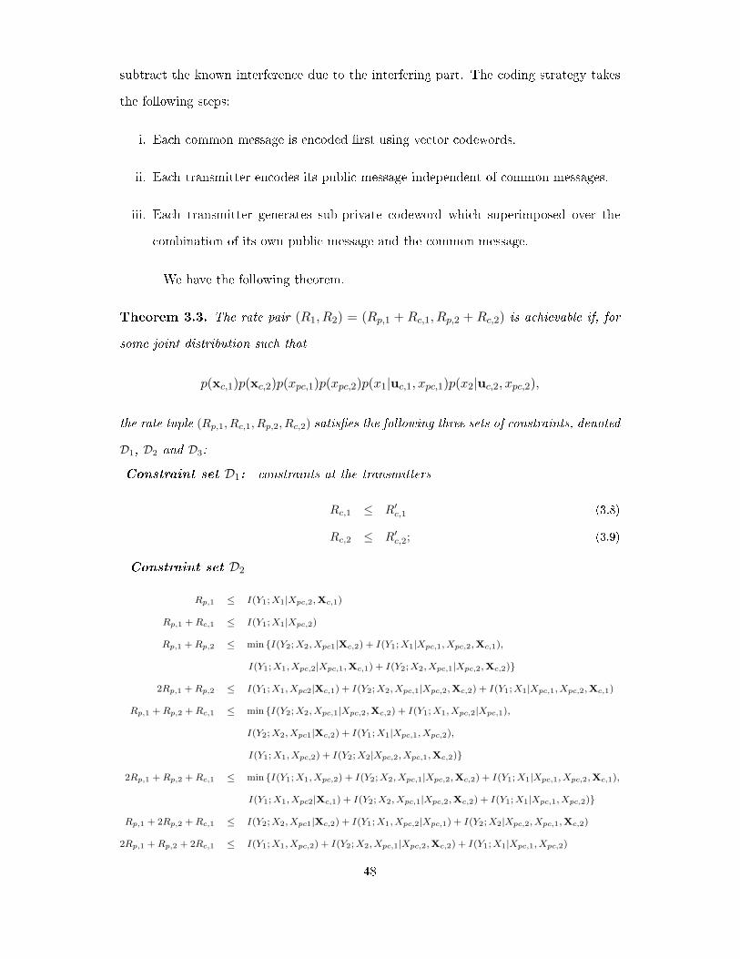
subtract the known interference due to the interfering part. The coding strategy takes
the following steps:
i. Each common message is encoded �rst using vector codewords.
ii. Each transmitter encodes its public message independent of common messages.
iii. Each transmitter generates sub-private codeword which superimposed over the
combination of its own public message and the common message.
We have the following theorem.
Theorem 3.3. The rate pair (R1, R2) = (Rp,1 + Rc,1, Rp,2 + Rc,2) is achievable if, for
some joint distribution such that
p(xc,1)p(xc,2)p(xpc,1)p(xpc,2)p(x1|uc,1, xpc,1)p(x2|uc,2, xpc,2),
the rate tuple (Rp,1, Rc,1, Rp,2, Rc,2) satis�es the following three sets of constraints, denoted
D1, D2 and D3:
Constraint set D1: constraints at the transmitters
Rc,1 ≤ R′c,1 (3.8)
Rc,2 ≤ R′c,2; (3.9)
Constraint set D2
Rp,1 ≤ I(Y1;X1|Xpc,2,Xc,1)
Rp,1 +Rc,1 ≤ I(Y1;X1|Xpc,2)
Rp,1 +Rp,2 ≤ min {I(Y2;X2, Xpc1|Xc,2) + I(Y1;X1|Xpc,1, Xpc,2,Xc,1),
I(Y1;X1, Xpc,2|Xpc,1,Xc,1) + I(Y2;X2, Xpc,1|Xpc,2,Xc,2)}
2Rp,1 +Rp,2 ≤ I(Y1;X1, Xpc2|Xc,1) + I(Y2;X2, Xpc,1|Xpc,2,Xc,2) + I(Y1;X1|Xpc,1, Xpc,2,Xc,1)
Rp,1 +Rp,2 +Rc,1 ≤ min {I(Y2;X2, Xpc,1|Xpc,2,Xc,2) + I(Y1;X1, Xpc,2|Xpc,1),
I(Y2;X2, Xpc1|Xc,2) + I(Y1;X1|Xpc,1, Xpc,2),
I(Y1;X1, Xpc,2) + I(Y2;X2|Xpc,2, Xpc,1,Xc,2)}
2Rp,1 +Rp,2 +Rc,1 ≤ min {I(Y1;X1, Xpc,2) + I(Y2;X2, Xpc,1|Xpc,2,Xc,2) + I(Y1;X1|Xpc,1, Xpc,2,Xc,1),
I(Y1;X1, Xpc2|Xc,1) + I(Y2;X2, Xpc,1|Xpc,2,Xc,2) + I(Y1;X1|Xpc,1, Xpc,2)}
Rp,1 + 2Rp,2 +Rc,1 ≤ I(Y2;X2, Xpc1|Xc,2) + I(Y1;X1, Xpc,2|Xpc,1) + I(Y2;X2|Xpc,2, Xpc,1,Xc,2)
2Rp,1 +Rp,2 + 2Rc,1 ≤ I(Y1;X1, Xpc,2) + I(Y2;X2, Xpc,1|Xpc,2,Xc,2) + I(Y1;X1|Xpc,1, Xpc,2)
48

Rp,1 +Rp,2 +Rc,1 +Rc,2 ≤ min {I(Y1;X1, Xpc,2|Xpc,1) + I(Y2;X2, Xpc,1|Xpc,2),
I(Y2;X2, Xpc,1) + I(Y1;X1|Xpc,1, Xpc,2)}
2Rp,1 +Rp,2 +Rc,1 +Rc,2 ≤ min {I(Y1;X1, Xpc,2) + I(Y2;X2, Xpc,1|Xpc,2) + I(Y1;X1|Xpc,1, Xpc,2,Xc,1),
I(Y1;X1, Xpc2|Xc,1) + I(Y2;X2, Xpc,1|Xpc,2) + I(Y1;X1|Xpc,1, Xpc,2)}
2Rp,1 +Rp,2 + 2Rc,1 +Rc,2 ≤ I(Y1;X1, Xpc,2) + I(Y2;X2, Xpc,1|Xpc,2) + I(Y1;X1|Xpc,1, Xpc,2);
Constraint set D3: Same as D2 with the indices �1� and �2� interchanged.
Proof. The proof is similar to the proof of Theorem 3.2, and is omitted.
3.4 The Gaussian Case with Symmetric Channel Gains
In this section, we illustrate the coding strategies discussed above for the case of a
second-hop modeled as a symmetric Gaussian interference channel; i.e., h1,1 = h2,2 = h
and h1,2 = h2,1 = g. We note that determining the complete rate region, optimal coding
schemes and input distributions for the interference channel is a complex task, and
does not yield much insights. Therefore, we restrict our attention to characterizing the
symmetric achievable rate, de�ned as R = maxmin {R1, R2}, where the rate pair (R1, R2)
belongs to the best known achievable rate region for the interference channel of interest.
Further, we limit our discussions to the speci�c signaling schemes, encoding/decoding
order, as will be discussed below.
Let the received signal at each receiver is given by
Y1 = hX1 + gX2 + Z1
Y2 = hX2 + gX1 + Z2,
where X1 and X2 are the transmitted signals from S1 and S2 respectively, and Zi ∼
N (0, 1), i = 1, 2, is the additive Gaussian noise at receiver Di. Each transmitter has a
power constraint E[|Xi[n]|2] ≤ P . We assume that each user has access to the same
amount of side-information, i.e., R′c,1 = R′
c,2 = R′c.
Before proceeding further with the coding strategies, we remark on the notation
used in this section. For convenience, we use Xa to denote any vector of the form
[Xa,1, Xa,2]. Further, we let h1 = [h, g], h2 = [g, h] and ∥h∥2 = h2 + g2. Observe that hi is
the vector channel formed by the transmitter (S1, S2) at the receiver Di .
49

Let (v1, vc,2) = (vpc,1, vpp,1, vc,1, vc,2) and (v2, vc,1) = (vpc,1, vpp,1, vc,1, vc,2) be the
message set to be transmitted from S1 and S2 respectively. Encoder 1 employs XNpc,1 to
encode vpc,1, UNpp,1 to encode vpp,1, and UN
c,1,1 and UNc,2,1 to encode vc,1 and vc,2 respec-
tively. Similarly, encoder 2 employs XNpc,2 to encode vpc,2, UN
pp,2 to encode vpp,2, and UNc,1,2
and UNc,2,2 to encode vc,1 and vc,2 respectively. Note that UN
c,1 and UNc,2 are generated
cooperatively by both encoders. Each encoder splits its power P into three parts, Pc,
Ppp and Ppc. All codewords are drawn from a zero mean Gaussian ensemble. Both
encoders compute Xc,1 = fc1(Uc,1,Uc,2), Xc,2 = fc2(Uc,1,Uc,2) and encoder Si computes
Xpp,i = fp,i(Upp,i) as the transmit signals. Then Si transmits
Xi = Xc,1,i +Xc,2,i +Xpc,i +Xpp,i
The received signal at Di can be written as
Yi = h†i (Xc,1 +Xc,2 +Xpc +Xpp) + Z1.
We let ζi = h†i (Xpc +Xpp)+Z1 where ζi is the equivalent additive noise at Di in decoding
the common messages, treating the interference due to private messages as additive noise.
Observe that ζi ∼ N (0, σ2ζ ), where σ
2ζ = 1 + ∥h∥2 Pp.
Binning for interference cancelation: layered dirty paper coding (DPC)
In this section we demonstrate the application of GP binning techniques which, when
specialized to the Gaussian case, boil down to dirty paper coding (DPC) [42]. Essen-
tially, DPC involves pre-cancelation of interference at the transmitter without incurring
any power cost. From the perspective of transmitting common information only, the
interference channel can be modeled as a Gaussian vector broadcast channel, except that
it has the interference due to private messages. Gaussian MIMO broadcast channels
have been well studied and their capacity regions have been characterized in [43, 57]
by exploiting DPC. Therefore, it is clear that DPC's performance in the second hop is
superior when entire information at relays is common.
Encoding:
1. Encoding the public messages: Encoder Si chooses a codeword XNpc,i, Xpc,i ∼
N (0, Ppc) to relay its own public message. Public messages are decoded �rst at the50

receivers, and their e�ects are subtracted from the received signals before decoding
common and sub-private messages.
2. Encoding the common messages: Relays collaborate to encode the common messages
sequentially. Suppose at any time the common message pertaining to one user is encoded,
DPC is performed on the common message of the other user treating the interference
due to the �rst user's common message as the known information. Consider the general
case, where relays L1 and L2 allocate Ppp,1 and Ppp,2 for the transmission of their private
messages. Then, it is clear that the sum power budget is 2P −Pp,1−Pp,2 for transmitting
common messages, where Pp,i = Ppp,i + Ppc,i. While the second-hop is analogous to a
vector BC, we should point out that, relay L1 has to use only P − Pp,1 and relay L2
has to use only P − Pp,2 to transmit the common information. We will develop a time
sharing mechanism to overcome this di�culty. Depending on the encoding order of the
common information, DPC is performed using following strategies.
• Encoding strategy π1 For private messages, set Ppp,1 = p∗1 and Ppp,2 = p∗2. Relays �rst
encode vc,2 using UNc,2(vc,2). Then, set XN
c,2 = UNc,2. Encode vc,1 using UN
c,1(vc,1), and
apply DPC on UNc,1(vc,1) treating XN
c,2 as the known interference while treating the e�ect
due to sub-private messages, ζN1 = h†1X
Npp + ZN
1 , as the noise. That is, choose the vector
Xc,1 ∼ N (0,Σc,1), independent of Xc,2, such that
Uc,1 = Xc,1 +BcXc,2,
where Bc is chosen as per the DPC requirement [42]; i.e., Bc corresponds to the optimal
non-causal MMSE estimate of Xc,1 given h†1Xc,1 + ζ1. Encoders jointly compute their
signals for relaying the common message set asXc = Xc,1+Xc,2. Relays choose covariance
matrices to maximize the sum-rate; i.e, Σ1 = Σπ11 , Σ2 = Σπ1
2 ; where {Σπ11 ,Σπ1
2 } is the
solution to (3.10).
Rπ1(p∗1, p
∗2) = max
Σ1,Σ2
(C
(h†1Σ1h1
1 + h2p∗1 + g2p∗2
)+ C
(h†2Σ2h2
1 + h†2Σ1h2 + h2p∗2 + g2p∗1
))(3.10)
subject to tr (Σ1 +Σ2) ≤ 2P − Ppc,1 − Ppc,2 − p∗1 − p∗2.
• Encoding strategy π2 For private messages, set Ppp,1 = p∗2 and Ppp,2 = p∗1. Relays encode
vc,1 in XNc,1, then generateX
Nc,2 by encoding vc,2 and then performing DPC treating h†
2XNc,1
51

as the known side information. As before, the optimal sum-rate, Rπ2(p∗1, p
∗2), is obtained
by solving (3.10) swapping indexes 1 and 2, with the corresponding covariance matrices
being {Σ1,Σ2} = {Σπ21 ,Σπ2
2 }.
• Time sharing Observe that the power allocation for common messages at each re-
lay, corresponding to the strategy πj , is determined by Pπj
c,1∆=[Σ
πj
1 +Σπj
2
]1,1
; Pπj
c,2∆=[
Σπj
1 +Σπj
2
]2,2. To meet the power constraint at each relay, relays perform time sharing
by using π1 for the �rst half of the slot and π2 for the second half. Note that, due to
symmetry in channel conditions, relay Li obeys the average power constraint per slot:
1
2(Pπ1
c,i + Pπic,1 + Ppc,1 + Ppc,2 + p∗1 + p∗2) = P.
3. Encoding the sub-private messages: Observe that, due to DPC, each user is able
to decode its own common message but not the interfering part. Therefore, the e�ect
of the common message due the other user is still interference. Fortunately, this is
known side-information to the encoders. Therefore, each encoder performs another
round of DPC on its own sub-private messages, treating the e�ect of interfering part of
the common codeword as the known side-information. To this end, Di chooses the DPC
signal Xpp,i ∼ N (0, Ppp), independent of Uc,j , j = i, such that,
Upp,i = Xpp,i + b†cUc,j ,
where bc corresponds to the MMSE estimator of Xpp,i given h†1Xpp,i+Zi. It is interesting
to note that bc does not depend on the variance of the interference. Therefore, due to
DPC, each individual receiver can decode its private message as though there were no
interference due to common messages.
Decoding: Receivers decode messages in the following order. Public messages are
decoded �rst, treating h†i (X
Nc,1+XN
c,2+XNpp), the interference from common messages and
private messages, as noise. Once the public messages are decoded, each receiver sub-
tracts their e�ect, h†iXpc, from the received signal, Yi. In the second step, each receiver
decodes the part of common message intended for it. In decoding the common message,
each receiver treats h†iX
Npp, the interference due to sub-private messages, as noise. Fi-
nally, receivers decode their sub-private messages individually, treating the interference
due to the sub-private message of other user as noise. Note that the interference from
52

public messages disappears due to interference cancelation at the receiver, and the inter-
ference from common messages is canceled out due to the DPC performed on sub-private
messages.
Analysis: Next, we evaluate the achievable rates due to this scheme. Let a power split
(Ppc, Pc, Ppp) at relays be given such that Ppc+Pc+Ppp = P . As mentioned earlier, public
messages are decoded �rst, treating the e�ect of common and sub-private messages as
noise. Therefore, the equivalent noise at receiver Di in decoding the public message is
given by
Ψi = h†i (Xc,1 +Xc,2 +Xpp) + Zd,i.
We note that Ψ ∼ N (0, σ2Ψ), where
σ2Ψ = E[|Ψ|2]
= h†i (Σ1 +Σ2 + Ppp · I)h†
i + 1
= ∥h∥2 (P − Ppc) +4Pcg
2h2
∥h∥2 + Pch2∆
σ2p
+ 1,
where σ2p = ∥h∥2 Ppp + 1.
Next, consider the transmission of common messages. For the general case, a
closed-form solution for the optimal power allocation is still unknown. However, under
the symmetric power allocation for the sub-private message set Ppp,1 = Ppp,2 = Ppp, it
can be shown that the optimal sum-rate is given by (see [58] for details)
Rπ1c = C
((h2 − g2)2P
2c
σ4p+
2Pc
σ2p∥h∥2
), (3.11)
and the corresponding DPC matrices are given by (refer to Appendix B.4, for more
details)
Σπ1c,1 =
Pc(σ2p1 +
Pcσ2p∥h∥2
)(∥h∥2 + Pc
σ2ph2∆
) h2
(1 + Pc
σ2ph∆
)2gh(1− Pc
σ2p
2h2∆
)gh(1− P ′
c2h2∆
)g2 (1− P ′
ch∆)2
,Σπ1c,2 =
Pc
(1 + 2Pc
σ2p∥h∥2 + P 2
cσ4p
)(1 + Pc
σ2p∥h∥2
)(∥h∥2 + Pc
σ2ph2∆
) g2 hg
hg h2
, (3.12)
where h2∆ = h2 − g2.
53

Next, consider sub-private messages. Observe that DPC is performed on the
private message treating the interference due to common information as the known
side-information. Further, each receiver subtracts out the interference due to public
messages. Therefore, each receiver can decode its own sub-private message as though
there were no interference due to common messages and public messages. Therefore,
each relay can transmit its private information at a rate
Rpp = C
(h2Ppp
1 + g2Ppp
). (3.13)
Therefore, when the proposed layered coding with DPC is used, the total achiev-
able rate per link is given by
RLAY−DPC = max{Ppc,Pc,Ppp:
Pc+Pp=P
}Rpc +Rc +Rpp; s. t. Rc ≤ R′c,
where Rc is the common information rate per link, Rpc is the public information rate
per link, and Rpp the sub-private information rate per link, given by
Rc =1
2C
((h2 − g2)2P
2c
σ4p+
2Pc
σ2p∥h∥2)
),
Rpc = min
{C
(g2Ppc
σ2Ψ
),1
2C
(∥h∥2 Ppc
σ2Ψ
)}, and Rpp = C
(h2Ppp
1 + g2Ppp
).
We remark that our choice of covariance matrices, in performing DPC for the
common messages, is greedy, in the sense that it maximizes the rates for transmission
of the common message without taking into account their e�ect on the public messages.
We observe that due to the above mentioned decoding order, apart from private mes-
sages, common messages also appear as interference for public messages. Since common
messages are aired using vector broadcast techniques, the signal power of the common
messages at the receivers is enhanced signi�cantly. Therefore, public messages may in-
cur signi�cant amounts of interference from common messages. Thus when Rc is large,
the contribution due to public messages vanishes, and consequently, it is bene�cial to
perform DPC without resorting to splitting the private message toward interference can-
celation. Indeed, when Rc and hence Pc increases, a small amount of power P1 = P −Pc
is left to rely private and public messages. Concordant to the results obtained for54

weak interference channels [59, 60, 61], when P1 satis�es P1 ≤ (h−2g)2g3 , splitting of the
private message is no longer necessary. Thus, to decoding one user's private message
while treating other user's private message as noise becomes optimal. When Rc is very
small, a relatively smaller amount of power is spent on transmitting common messages.
Therefore, it is bene�cial to perform message splitting of the private message to aid in
interference cancelation.
Superposition coding: layered beamforming
In the previous section, we proposed a layered coding strategy that incorporates DPC
to relay common messages. However, we note that DPC has high complexity. The
non-linearity inherent in DPC inhibits us from avoiding interference due to the common
messages when decoding public messages. This may not be bene�cial always. On the
other hand, linear schemes like beamforming are much easier to implement, and reduce
the burden of common messages before decoding the private messages. In light of the
above observations, we propose coding schemes based on a marriage of HK coding and
BF schemes.
Strategy I: As noted in the previous section, this scheme requires each receiver to
decode both the common messages. Since information rate in such cases is determined
by the weaker link, this scheme yields bene�ts when the gain on the interfering link is
higher.
Encoding: For transmitting common messages, transmitters apply coherent beam-
forming by letting each encoder choose its symbols such that Uc,1,1 = Uc,1,2 = Uc,1 and
Uc,2,1 = Uc,2,2 = Uc,2, with Uc,i ∼ N (0, 1), i = 1, 2. That is, Σu,1 = Σu,2 =
1 1
1 1
. Then,set
Xc,1,1 =√PcmUc,1; Xc,2,1 =
√PcuUc,2
Xc,1,2 =√PcuUc,1; Xc,2,2 =
√PcmUc,2
where Pcm and Pcu are chosen such that Pc = Pcm+Pcu. Observe that Pcm is the portion of
the power used by each transmitter to transmit the intended part of its common message,
while Pcu is the power used to transmit the �interfering part� as the side-information.
55

For transmitting public and sub-private messages, each encoder uses codewords XNpc,i
and XNpp,i respectively. To transmit its message set, transmitter i computes the signal
Xi as
Xi = Xc,1,i +Xc,2,i +Xpc,i +Xpp,i, i = 1, 2.
Observe that E[|Xi|2] = P .
Decoding: Receivers decode messages in the following order. First, each receiver
decodes common information. To decode the common information, the e�ect of private
messages is treated as noise. Once the common messages are decoded, each receiver
subtracts the e�ect of the common messages from its received signal in order to decode
its private messages Thus, there is no interference from the common messages on the
private messages. Observe that each splitting of private message into sub-private and
public sub-messages is according to HK coding.
Analysis: We represent the received signal as
Yi = h†i (Xc,1 +Xc,2 +Xpc +Xpp) + Zi.
Considering the transmission of only common messages, we equivalently model the chan-
nel as
Y1 = h†1aUc,1 + h†
2aUc,2 + ζ1, (3.14)
where, for convenience, we have de�ned a = [√Pcm,
√Pcu]. Furthermore, ζ1 is the equiv-
alent noise at D1 in decoding the common messages, with ζd,1[n] ∼ N (0, σ2ζ ), where
σ2ζ = ∥h∥2 Pp + 1.
Similarly, for the second receiver D2,
Y2 = h†1aUc,2 + h†
2aUc,1 + ζ2, (3.15)
where ζ2 ∼ N (0, σ2ζ ).
Consider the transmission of common information. We observe that (3.14) rep-
resents a virtual MAC formed by (Uc,1, Uc,2, Y1), and (3.15) represents another virtual
MAC formed by (Uc,1, Uc,2, Y2). The achievable common information rate region is the
intersection of the regions formed by these two MACs. The following proposition gives
the optimal power allocation vector for the common information transmission.56

Proposition 3.1. The common information rate per link, under coherent beamforming,
is maximized by equal power allocation at the relays, given by Pcm = Pcu = Pc/2, and
the corresponding common information rate per link is given by
Rc =1
2C
((g + h)2 Pc
∥h∥2 Pp + 1.
). (3.16)
The proof can be found in Appendix B.3.
Next, consider the private messages. Since sub-common messages and sub-
private messages are decoded by canceling the interference due to the common messages,
the encoding and decoding of the public and sub-private messages mimic the version of
HK coding considered in [14]. The information rate for the private message for each
user is given by
Rp = max{Ppc,Ppp:
Ppc+Ppp=Pp
}Rpp +Rpc, (3.17)
with
Rpp = C
(h2Ppp
1 + g2Ppp
)and Rpc = min
{C
(g2Ppc
1 + ∥h∥2 Ppp
),1
2C
(∥h∥2 Ppc
1 + ∥h∥2 Ppp
)}.
Thus, the rate that can be achieved per user in the second hop due to CBF is
RCBF = max{Pc,Pp:
Pc+Pp=P
}Rp +Rc; s. t. Rc ≤ R′c.
Strategy II:
In the coherent beamforming case, each receiver needs to decode all the common mes-
sages. This might restrict the rate of common information when the interference is
moderately low. Under these circumstances, it can be bene�cial to relax this require-
ment which is in spirit with the strategy II discussed in Section 3.3. For the Gaussian
case, the design of an optimal beamforming vector for the common message codewords is
crucial. In our illustration, for simplicity, we consider zero forcing beamforming (ZFBF),
which involves transmitters pre-subtracting the known interference due to the interfer-
ing part of the common message. Essentially, ZFBF consists of inverting the channel
matrix by the relays to create orthogonal channels between the relays and the receivers.
Encoding: For transmitting common messages, each encoder chooses its symbols such57

that Uc,1,1 = Uc,1,2 = Uc,1 and Uc,2,1 = Uc,2,2 = Uc,2, with Uc,i ∼ N (0, 1), i = 1, 2. That is,
Σu,1 = Σu,2 =
1 1
1 1
. Then, setXc,1,1 =
h√Pc
∥h∥Uc,1; Xc,2,1 = −
g√Pc
∥h∥Uc,2
Xc,1,2 = −g√Pc
∥h∥Uc,1; Xc,2,2 =
h√Pc
∥h∥Uc,2
For transmitting public and sub-private messages, each encoder uses codewords XNpc,i
and XNpp,i respectively. To transmit its message set, transmitter i computes the signal
Xi as
Xi = Xc,1,i +Xc,2,i +Xpc,i +Xpp,i, i = 1, 2.
Observe that E[|Xi|2] = P .
Decoding: Receivers decode messages in the following order. First, each receiver
decodes the common information. Observe that each user is able to decode only his own
common message and the interfering part of the common messages vanishes due to zero-
forcing. To decode the common information, the e�ect of private messages is treated as
noise. Once the common messages are decoded, each receiver subtracts the e�ect of the
common messages from its received signal in order to decode its private message. Thus,
there is no interference from the common messages on the private messages. Observe
that each splitting of private message into sub-private and public sub-messages is similar
to HK coding.
Analysis: With the decoding order �xed as mentioned above, the rate of common
information per user is given by
Rc = C
( (h2 − g2
)2Pc
∥h∥2 (1 + ∥h∥2 Pp)
). (3.18)
The information rate for the private message per user is given by
Rp = max{Ppc,Ppp:
Ppc+Ppp=Pp
}Rpp +Rpc, (3.19)
with
Rpp = C
(h2Ppp
1 + g2Ppp
)and Rpc = min
{C
(g2Ppc
1 + ∥h∥2 Ppp
),1
2C
(∥h∥2 Ppc
1 + ∥h∥2 Ppp
)}.
58

Thus, the rate that can be achieved per user in the second hop due to ZFBF is
RZFBF = max{Pc,Pp:
Pc+Pp=P
}Rp +Rc; s. t. Rc ≤ R′c.
3.5 Numerical Examples
We perform numerical evaluation of the schemes discussed above. The metric of interest
is the total achievable symmetric rate per user. For ease of evaluation, we consider
a symmetric interference L → D link with a link SNR of 20dB, where we de�ne link
SNR = h2P . We are interested in studying the e�ect of common information availability,
Rc at the relays, on the achievable information rate per user ILD over the L → D
link. De�ne the parameter α = g2/h2. Figs. 3.2 and 3.3 show ILD versus Rc plots
for di�erent schemes. For comparison purposes, we also consider the naive strategies
without layering: HK-scheme (does not exploit the common information), DPC and
beamforming (do not split private message for interference cancelation). The optimal
power allocation policies and the corresponding achievable rates of di�erent schemes
were determined numerically by exhaustive search.
We have the following observations:
• Layered coding with DPC outperforms all other schemes for all ranges of Rc ex-
amined and for relatively small values of α. This is because, for relatively smaller
values of α's, the interference of common messages on public messages is low, en-
0 0.5 1 1.5 2 2.5 3 3.5 4
1.4
1.6
1.8
2
2.2
2.4
2.6
2.8
3
3.2
Common Information from first hop , Rc (bits/s/Hz/user)®
Rat
e in
the
seco
nd h
op, I
LD (
bits
/s/H
z/us
er)®
HK−schemeCBFZFBFDPCLAY−BFLAY−DPC
Figure 3.2: ILD vs. Rc curves (α = 0.2).
0 0.5 1 1.5 2 2.5 3 3.5 40.5
1
1.5
2
2.5
3
Common Information from first hop , Rc (bits/s/Hz/user)®
Rat
e in
the
seco
nd h
op, I
LD (
bits
/s/H
z/us
er)®
HK−schemeCBFZFBFDPCLAY−BFLAY−DPC
Figure 3.3: ILD vs. Rc curves (α = 0.6).
59

abling e�cient message splitting for smaller values of Rc. When Rc is large, the
layered coding scheme boils down to DPC which is optimal when Rc is large.
• Layered coding with BF is superior to its DPC counterpart for larger values of α
in the regime when Rc is small. While both DPC and BF enhance the SNR of the
common messages, for the layered DPC scheme, the interference due to common
messages may drastically a�ect the rate of the public messages to an extent that
it may become bene�cial for relays to allot more power to transmitting the private
message than to transmitting the common messages. However, for the layered
BF scheme, successive cancelation of interference from common messages at the
receivers proves to be useful.
• HK based scheme outperforms DPC and BF schemes when the amount of common
information available is relatively low. This indicates that in such cases, it is ben-
e�cial to allocate more power for unknown interference cancelation than relaying
the common information.
• The performance of layered coding schemes boils down to that of HK coding when
there is no side information available at the relays; i.e., Rc = 0. This is due to
the fact that HK coding is the best known scheme for ICs where the transmitters
have no side information.
• The beamforming method is not superior in any regime. For higher values of α,
performance of CBF improves whereas the performance of ZFBF becomes worse.
When the values of α is low, ZFBF performs better when compared to the CBF.
This is due to the fact that the power spent on the information bits in ZFBF
decreases with the interference and the gain due to coherent combining in CBF
increases with the strength of interfering link.
3.6 Conclusions
In this chapter, we considered a basic model for two-hop transmissions of two informa-
tion �ows that interfere with each other. The main focus has been on the second hop
60

transmission, where one intrinsic feature is that each relay has access to a part of the in-
formation intended for the other destination. A key observation is that when each relay
has only partial side-information, neither distributed MIMO broadcast nor HK coding
would be optimal, and a naive combination of these two schemes would not work either.
Further, since each receiver receives a superposition of di�erent sub-messages that are
relayed, the decoding order of the signals at the receiver plays a critical role. Therefore,
e�cient relaying strategies entail a careful marriage of distributed MIMO broadcast and
HK coding.
We addressed the above challenge by investigating di�erent relaying schemes and
developing novel layered strategies built on distributed MIMO broadcast and HK coding.
Speci�cally, we proposed two types of layered schemes: layered coding with binning and
layered superposition coding. We illustrated the applications of proposed strategies for
a symmetric Gaussian case. We presented numerical examples to demonstrate that our
schemes can yield a substantial rate gain.
61

Chapter 4
WHEN COMPRESSIVE SAMPLING MEETS MULTICAST: OUTAGE ANALYSIS
AND SUBBLOCK NETWORK CODING
4.1 Introduction
Multicasting is an emerging technology in wireless networks in supporting a plethora of
applications, including text, teleconferencing, and multimedia streaming, to a group of
users. Notably, many of these signals are known to be sparse or compressible, where
the sparsity (or compressibility) refers to the property that the �essential information
rate� of a signal is signi�cantly smaller than what is suggested by its bandwidth (in
case of continuous signals), or that a signal essentially depends on a number of degrees
of freedom which is much smaller than its length (in case of discrete-time signals).
Images, for instance, usually admit a compact representation in the wavelet domain,
and audio signals can be often compressed in the frequency domain. As a result, in
data communication systems, data transmission is often preceded by its compression, to
ensure e�cient utilization of resources by minimizing redundancy.
As shown in Fig. 4.1(a), the conventional method of data compression involves
sampling the signal at the Nyquist rate, storing the samples, and compressing them in
an appropriate domain prior to the transmission. One �drawback� of the traditional
approach when applied to sparse signals is that the size of measurements is of the same
order as of the size of the signal itself, independent of its sparsity/compressibility. This
would incur heavy sampling and storage burden at the sender. On the other hand, recent
developments in compressive sensing theory [19, 20, 21] have provided methods not only
for lower-rate signal acquisition, but also for accurate signal reconstruction, as shown
in Fig. 4.1(b). One basic idea behind compressive sensing theory is that it exploits
the compressibility of the signals by only sensing its essential information. We note
that a scheme involving compressive sensing was considered in [62], for point-to-point
transmission.
In this study, a primary objective is to understand the reliable delivery of com-
pressible information to many destinations over wireless channels. This transmission sce-
62

nario, for instance, is useful for multimedia streaming over a WiFi or WiMAX network
with multiple receivers. It is also applicable to sensor networks, where each sensor node
wishes to communicate its sensed observations to multiple coordinating agents. Need-
less to say, this problem is quite challenging due to the lossy nature of wireless channels
and the heterogeneity in the amount of information received across di�erent receivers.
Another challenge is the �bottleneck� e�ect with the shared transmission medium among
many receivers, i.e., the overall performance is limited by the receiver that has the worst
channel condition. Therefore, ensuring that the QoS for the bottleneck user is on par
with the others clearly makes the multicast transmission more challenging.
We note that traditionally, in order to mitigate data loss over wireless channels,
retransmission schemes are widely used, e.g., Automatic Repeat reQuest (ARQ) [63].
However, retransmissions would not work well in some practical situations, particularly,
in multicast scenarios with many destinations (receivers) [64] or when the applications
are delay sensitive. Alternatively, forward error correction (FEC) can be used to reduce
the amount of feedback [65], but a signi�cant challenge in using FEC is to determine the
right amount of redundancy because too much FEC redundancy would unnecessarily
slow down the data dissemination process, whereas insu�cient redundancy leaves many
receivers unable to decode the information. Furthermore, the inherent heterogeneity of
information conveyed to multiple receivers signi�cantly complicates the task of redun-
dancy estimation. Notably, network coding (NC), a recent breakthrough by Ahlswede
et al. [18], o�ers a promising platform for multicast transmissions. With this insight,
we will study joint compressive sensing and network coding for multicasting compressive
signals, as illustrated in Fig. 4.1(c). To the best of our knowledge, there has been little
e�ort on exploring compressive sensing over a multicast scenario; and this work is among
the �rst few to examine the interplay between compressive sensing and network coding.
Speci�cally, we consider a single-hop wireless network in which the sender mul-
ticasts a compressively sensed signal to L receivers, over wireless channels. We note
that many natural and man-made signals can be modeled as power-law decay signals,
a class of signals whose coe�cients decay according to the power law, when sorted in
the decreasing order. (For example, video signals admit power-law decay in the wavelet
63

domain.) Without loss of generality, we assume that the compressible signal belongs to
the class of power-law decay signals. We are particularly interested in the distortion of
the reconstructed signal, in terms of the mean squared error (MSE), at each individual
receiver. For a given target MSE, we shall characterize the outage probability, where
the outage is de�ned as the event in which the MSE in signal reconstruction exceeds
the target MSE. Due to multiple receivers, the network outage is dominated by the
�bottleneck� receiver.
Roughly speaking, depending on the computing capability of senders and re-
ceivers, there are two possible approaches for transmitting the compressible data: (A)
transmit raw measurements or (B) transmit the compressed coe�cients. Approach (A)
of transmitting raw samples is more applicable to situations where senders are less so-
phisticated than the receivers, e.g., in a sensor network where a sensor multicasts its
sensed observation to multiple coordinating agents. A typical sensor node, being a tiny
and battery-operated device, could not a�ord sophisticated on-board data processing.
Further, since several sensor nodes are deployed in the network and many of them are
frequently refreshed/replaced, it might become highly costly for each sensor node to be
cognizant of the underlying signal structure. In this case, a plausible approach is to
transmit the compressed samples, as illustrated in Fig. 4.1(b). It is clear that, in this
scheme, the onus of faithful reconstruction of the compressive signal lies with the re-
ceiver, and the sender just needs to sample the source signal using an appropriate kernel
prior to the transmission. A signi�cant advantage is that a random sampling kernel (or
sampling matrix) at the sender often su�ces and no knowledge about the source signal's
structure is needed. In contrast, in Approach (B), the sender samples the signal, stores
it, compresses it in an appropriate domain, and transmits the compressed data to the
receiver. In this case, the sender needs to be cognizant of the signal structure and be
su�ciently sophisticated to carry out the data compression, e.g., as seen in multimedia
streaming in wireless networks and television broadcasting. Obviously, Approach (B)
would outperform Approach (A). Nevertheless, Approach (A) has the advantage that it
entails no strict requirements on the computational power at the sender.
In our study, we consider both approaches outlined above. First, we analyze
64

the outage performance corresponding to di�erent transmission strategies, and quantify
the behavior of the outage probability as a function of key parameters, including the
signal structure, channel erasure, and the number of receivers. As expected, when the
sender has the capability to sample and compress the signal before transmitting the
coe�cients, the required number of transmissions can be greatly reduced to meet the
outage requirement.
Next, we explore subblock network coding, a new network coding method tailored
towards transmitting power-law decay signals. This is motivated by the observation that
the traditional network coding could result in undesirable performance for power-law de-
cay signals. Then, we formulate the subblock network coding as an integer programming
problem, and develop a heuristic algorithm that exploits the inherent priority structure
of the power-law decay signal. We show that by using the proposed subblock network
coding scheme, one can gain substantially in terms of reconstruction performance when
compared to the traditional network coding.
In related work, recent developments in compressive sensing theory have spurred
a wide range of interest in di�erent applications of compressive signals [19, 20, 66]. In
particular, there have been some recent advances dealing with the applications of com-
pressive sensing in communications, and the transmission of compressible signals over
wireless channels. The transmission of compressible data over wireless channel has been
considered in [67, 68] which focus on the estimation of sensor data under a joint source-
channel coding framework and analyze the power-latency relationship with the number
of nodes. We note that, these works do not consider multicasting and the e�ect of
channel erasures. Along a di�erent avenue, network coding has received much attention
since the pioneering work of Ahlswede et al. [18]. In particular, in the context of reliable
multicast of data over wired networks, Ho et al. [69] have proposed a random linear
network coding used at an intermediate node to generate the coded packets. By doing
this, the authors have shown that the network capacity can be achieved asymptotically.
Recently, network coding has also been applied successfully to increase throughput in
wireless networks [70, 71]. In these works, by appropriately combining transmission
packets, the sender can reduce the number of required transmissions. Also, Nguyen et
65

Sampling Channel Coding
Receiver 1
Receiver L
Lossy
channels
State Information Feedback
Source
Coding
(a)
Compressive
Sampling
Receiver 1
Receiver L
Lossy
channels
State Information Feedback
(b)
Compressive
SamplingNetwork Coding
Receiver 1
Receiver L
Lossy
channels
State Information Feedback
Signal
Reconstruction
(c)
Figure 4.1: Multicast transmission of compressible data (a) conventional method; (b)transmission of compressed measurements (c) proposed joint compressive sensing andnetwork coding.
al. [72] have proposed an XOR-based network coding for single-hop wireless broadcast
networks to reduce the number of retransmissions. In contrast to these works, we in-
vestigate subblock network coding for transmitting power-law decay signal in multicast
networks. The work related most to ours is that of Stankovic et al. [73]. However, this
work studied only unequal error protection algorithms for progressive image transmission
in unicast transmissions.
The organization of this chapter is as follows. We provide in Section 4.2 the
system model and some background. In Section 4.3, we investigate in detail a variety of
transmission strategies and analyze the corresponding outage performance. In Section
4.4, we explore subblock network coding for power-law decay signals. Numerical results
and discussions are presented in Section 4.5. Finally, we draw conclusions in Section
4.6.
66

4.2 System Model and Background
We consider a multicast network where a sender wishes to transmit compressible signals
to L receivers over lossy wireless channels. Let x ∈ RN be the source signal of interest.
For example, x can be an audio/video signal in the context of multimedia and television
networks, or it can be a sensed physical stimulus at a sensor node in the context of sensor
networks. The link between the sender and each receiver is lossy; i.e., each transmitted
packet to a receiver Rj is subject to an erasure with probability ϵ. We assume that the
system is time-slotted and each slot length corresponds to one packet transmission.
Each receiver is required to meet a certain target MSE. We say that an outage
occurs, at receiver Rj , if the corresponding MSEj exceeds the target MSE. The outage
probability determines the QoS for each receiver. For a given target MSE, say mse, the
outage probability is given by
P jout = P(MSEj > mse), j = 1, . . . , L.
For convenience, we say there is a network outage when at least one of the
receivers su�ers an outage, i.e., {∃j ∈ {1, . . . , L} : MSEj > mse}. Accordingly, the network
outage probability can be given by
P ∗out = P(max
jMSEj > mse).
Clearly, the outage performance is governed by the receiver with the worst channel
conditions, i.e., the �bottleneck� receiver.
Next, we brie�y remark on the structure of the source signal under consideration.
Suppose that x ∈ RN , in some N−dimensional orthonormal basis Φ = {ϕ}Nn=1, ϕn ∈
RN , can be represented as
x =N∑
n=1
θnϕn, θn = ⟨x, ϕn⟩.
The vector θθθ = [θ1, . . . , θN ]T , is the coe�cient vector of x in the basis Φ. We
assume that x belongs to the class of power-law decay signals, in Φ, in the sense that
its coe�cients in this basis Φ decay according to a power-law, which is formally de�ned
as follows [19].67

Let x ∈ RN , and, for some orthonormal basis Φ, assume that the coe�cients
{θ}Nn=1 : θn = ⟨x, ϕn⟩ are re-indexed in a descending order such that
|θ(1)| ≥ |θ(2)| ≥ . . . |θ(n)|.
Then, we have the following de�nition.
De�nition 2.1. A signal x is a power-law decay signal in the orthonormal basis Φ, if
the vector θθθ obeys power-law decay, that is,
|θ(n)| ≤ Rn− 1
p , R > 0, for some �xed p ∈ (0, 1]. (4.1)
The corresponding error due to the best K−term approximation, x(K) ∆=∑K
k=1 θ(k)ϕ(k),
is given by
MSE(K) =∥∥∥x− x(K)
∥∥∥2 =N∑
n=K+1
|θ(n)|2 ≤ CrK−r, r =
2
p− 1,
where Cr = CpR2 and Cp depends only on p.
Power-law decay signals admit compressibility in the sense that the MSE in their
best K−term approximation can always be upper bounded by CrK−r.
We now restate an important result of compressive sensing regarding the recon-
struction of power-law decay signal x. In assessing the practical signi�cance of power-
law decay signals, a natural question arises; i.e., can we reconstruct the power-law decay
signal, x, with arbitrarily small reconstruction error with only a few number of measure-
ments of x? It turns out that the answer is positive. An important result by Candes
et al. [21] asserts that, with only O (K logN) random measurements (i.e., measurement
matrices are random matrices with i.i.d. entries) from a of x, one can reconstruct x with
MSE ≤ CrK−r. For the sake of completeness, we present the following result [21].
Theorem 4.1. (Optimal recovery of power-law decay signals from random measure-
ments) Suppose that x ∈ RN is a power-law decay signal in the basis Φ obeying (4.1)
for some �xed 0 < p < 1, and let a > 0 be a su�ciently small number. Assume that we
are given M = O(K logN) random measurements of x: y = Ψx, where Ψ is the M ×N
measurement matrix. Then with probability 1, the minimizer θθθ∗ to the optimization
68

problem
minθθθ∈RN
|θθθ|ℓ1
s. t. y = ΨΦθθθ
is unique. Furthermore, with probability at least 1−O(N− ρa ), we have
∥x− x∗∥2 ≤ Cp,aR2K−r, r = 2/p− 1.
Here, Cp,a is a �xed constant depending on p and a, but not on anything else. The
implicit constant in O(N−ρ/a) is allowed to depend on a.
The above theorem asserts that the power-law decay signals can be �sampled
accurately� using the techniques of compressive sensing.
Without loss of generality, we assume that the coe�cients of x follow the order:
|θ1| ≥ |θ2| ≥ . . . ≥ |θN |. Further, we assume that, prior to transmissions, the data
are quantized and encapsulated into packets. Since this study aims at obtaining a
fundamental understanding of the interplay between compressive sensing and network
coding, we assume that data quantization errors are negligible, which could be accounted
for further by using the same method in [74].
4.3 Transmission Strategies: Outage Analysis
In this section, we investigate in detail a variety of strategies for multicasting com-
pressible data to many receivers, depending on whether the transmitter is capable of
reconstructing the compressively sensed signal.
Transmission of compressed measurements (TCM)
In this method, the sender performs the compressed measurements of the source signal
using an M × N (M << N) sensing matrix Ψ. Each measurement is quantized with
a �ne precision and transmitted in the form of a packet. This scenario is of interest
where the sender could not a�ord the sophistication to reconstruct the source signal
from compressed measurements via ℓ1 optimization, and the receiver takes on more
processing burden. Further, in this case, the sender does not even need to know the
69

compressible basis of the source signal. This is typical in the case of sensor networks,
where the tiny sensor node has less computational power and is oblivious of the structure
of the source signal. The system diagram is illustrated in Fig. 4.1(b). In this case, the
sender transmits the raw, compressed measurements that are obtained via compressive
sensing, as outlined in [21].
Let K be the desired level of sparsity, and M = c1K logN be the corresponding
threshold on the number of measurements for reconstruction of the signal with the
desired accuracy. Let y be the M -length measurement vector obtained by sensing x
using M × N measurement matrix Ψ, i.e., y = Ψx, where Ψ is chosen such that the
solution to the ℓ1 optimization problem (4.2) will enable a satisfactory reconstruction of
the signal x in the sense of Theorem 4.1. It has been shown in [21] that this is possible
as long as the measurement matrix, Ψ, obeys a Uniform Uncertainty Principle (UUP)
and Exact Reconstruction Principle (ERP). Matrix Ψ should be chosen so as to capture
su�cient information with a high probability. More importantly, it is easy to �nd such
a projection matrix Ψ, since easily constructible ensembles like binary, Gaussian and
Fourier ensembles obey both UUP and ERP with high probability. Thus, in our case,
we assume that Ψ is generated by drawing its elements, independently and identically,
from a zero mean Gaussian distribution, i.e.,[Ψ]i,j ∼ N (0, 1N ).
LetM > Mcs be the number of measurements transmitted. Let Xjm be a random
variable representing the event of loss of the mth packet at the jth receiver. Xjm is a
binary random variable given by Xjm ∼ Bin(ϵ). Let Nj =
∑Mm=1X
jm, i.e., the number
of samples lost due to erasure at receiver Rj . Then, Nj is a binomial random variable
with parameters (M, ϵ). Observe that the outage is the event when a receiver loses more
than M −Mcs samples, i.e.,
P jout = P (Nj > M −Mcs) .
Next, we evaluate the outage probability of the �bottleneck� receiver:
P ∗out = P
(max
jNj > M −Mcs
).
Since M is large, it is reasonable to approximate Nj as a Gaussian random variable.
70

De�ne N∗j =
Nj−E[Nj ]√V ar(Nj)
. It follows that, N∗j ∼ N (0, 1). Then, we have
P ∗out = P
(max
jNj ≥M −Mcs
)= 1− P
(max
jN∗
j ≤M1
), (4.2)
where M1 =M(1− ϵ)−Mcs√
ϵ(1− ϵ)M.
Next, we need the following result from extreme value theory [75]: Let N∗1 , . . . N
∗L
be i.i.d. with N∗1 ∼ N (0, 1), aL and bL be two sequences of numbers such that aL →
∞, bL → 0, as L→∞. In particular,
aL =√
2 logL− 1
2(2 logL)−
12 (log(4π) + log logL) ,
bL = (2 logL)−12 .
Then,maxj N
∗j − aL
bL
D=⇒ ζ,
whereD=⇒ denotes convergence in distribution, and ζ(x) = exp(−e−x) is the Gumbel
CDF. Thus, we conclude that, as L→∞,
P(max
jN∗
j ≤M1
)=⇒ζ
(M1 − aL
bL
).
Based on (4.2), we obtain the outage probability as
P ∗out = 1− ζ
(M1 − aL
bL
).
For convenience, de�ne M2∆=M1 − aL
bL. Equivalently,
M2 =M1
√2 logL− 2 logL− 1
2log(4π logL).
Then, we can represent the outage probability as
P ∗out = 1− exp(−e−M2). (4.3)
After some algebra, it follows that
P ∗out ≈ 1− exp
−e−(1−ϵ−Mcs
M√ϵ(1−ϵ)
√2M logL−2 logL
). (4.4)
71

Observe that, in many practical scenarios,M is larger than L. We can then approximate
(4.4) as
P ∗out ≈ exp
(−
[1− ϵ− Mcs
M√ϵ(1− ϵ)
√2M logL− 2 logL
]). (4.5)
Observe that, for a �xed value of L, P ∗out decays exponentially with the square root of
the number of samples M .
Transmission of coe�cients (TC)
In this transmission strategy, the sender performs compressed sensing of x via measure-
ment matrix Ψ, and then estimates the K largest elements of the coe�cient vector θθθ.
That is to say, the sender is assumed to be capable of bearing the computational burden
of signal reconstruction via compressed measurements. Furthermore, each coe�cient is
quantized and encapsulated in a packet. There are a variety of ways in which these coef-
�cients can be protected against the channel erasure. To address this issue, we consider
several coding methods for the transmission of coe�cients.
Round robin transmission of coe�cients (TC-RR):
In this �naive� scheme, the sender transmits Kt packets with K coe�cients being trans-
mitted in a round-robin fashion with t repetitions. We assume that O(K logN) mea-
surements are made at the sender to obtain a K-term approximation for x. Without loss
of generality, we assume that the coe�cients θ1, . . . , θK are transmitted t times each.
For ease of exposition, �rst consider the case when t = 1. The number of packets
received by the receiver Rj is given by Nj =∑K
k=1Xjk. Further, the kth packet received
is denoted by θjk = Xjkθk. The MSE due to this scheme can then be upper bounded as
follows:
MSEj =N∑k=1
|θk − θjk|2
≤K∑k=1
|θk −Xjkθk|
2 + CrK−r.
Observe that
|θk −Xjkθk|
2 =
0 w. p. 1− ϵ
|θn|2 w. p. ϵ.
72
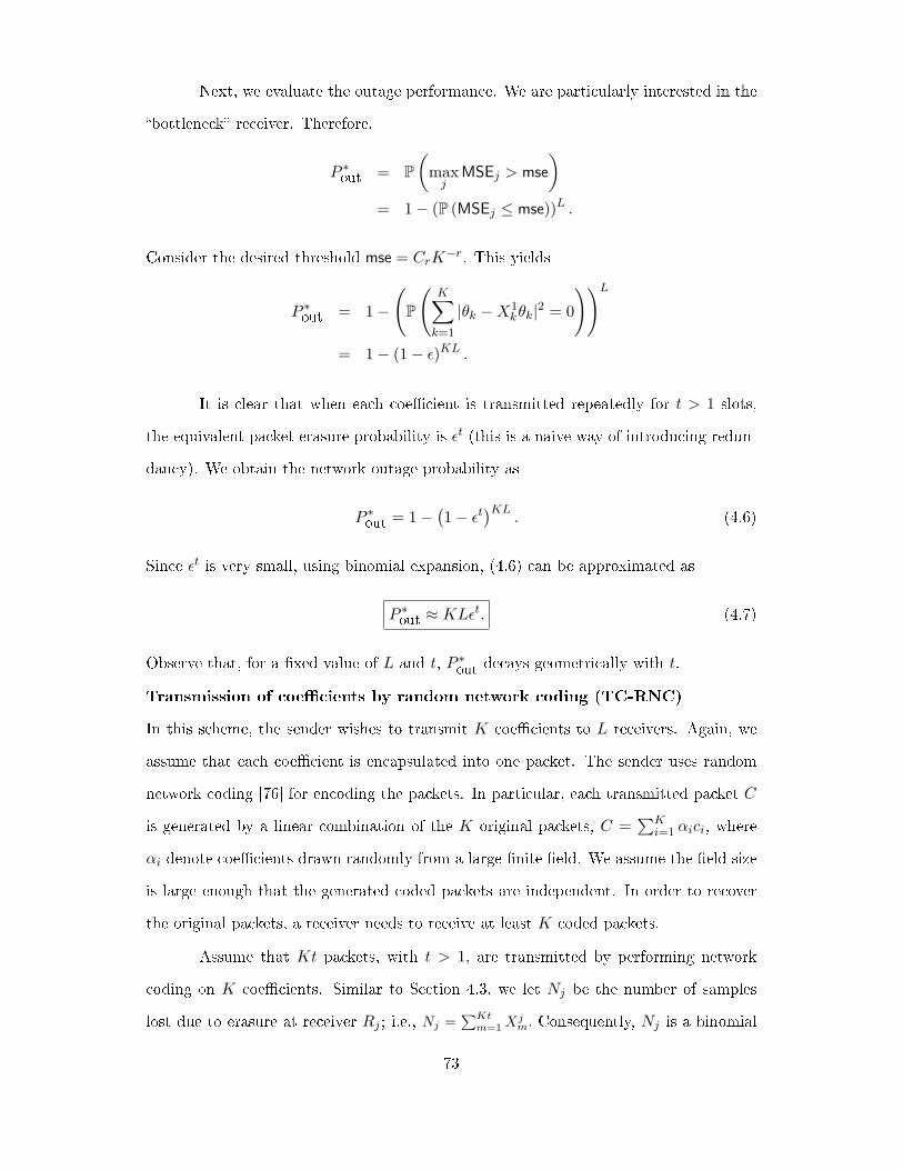
Next, we evaluate the outage performance. We are particularly interested in the
�bottleneck� receiver. Therefore,
P ∗out = P
(max
jMSEj > mse
)= 1− (P (MSEj ≤ mse))L .
Consider the desired threshold mse = CrK−r. This yields
P ∗out = 1−
(P
(K∑k=1
|θk −X1kθk|2 = 0
))L
= 1− (1− ϵ)KL .
It is clear that when each coe�cient is transmitted repeatedly for t > 1 slots,
the equivalent packet erasure probability is ϵt (this is a naive way of introducing redun-
dancy). We obtain the network outage probability as
P ∗out = 1−
(1− ϵt
)KL. (4.6)
Since ϵt is very small, using binomial expansion, (4.6) can be approximated as
P ∗out ≈ KLϵ
t. (4.7)
Observe that, for a �xed value of L and t, P ∗out decays geometrically with t.
Transmission of coe�cients by random network coding (TC-RNC)
In this scheme, the sender wishes to transmit K coe�cients to L receivers. Again, we
assume that each coe�cient is encapsulated into one packet. The sender uses random
network coding [76] for encoding the packets. In particular, each transmitted packet C
is generated by a linear combination of the K original packets, C =∑K
i=1 αici, where
αi denote coe�cients drawn randomly from a large �nite �eld. We assume the �eld size
is large enough that the generated coded packets are independent. In order to recover
the original packets, a receiver needs to receive at least K coded packets.
Assume that Kt packets, with t > 1, are transmitted by performing network
coding on K coe�cients. Similar to Section 4.3, we let Nj be the number of samples
lost due to erasure at receiver Rj ; i.e., Nj =∑Kt
m=1Xjm. Consequently, Nj is a binomial
73

random variable with parameters (Kt, ϵ). Since Kt is large, we have the approxima-
tion Nj ∼ N (Ktϵ, ϵ(1− ϵ)Kt) . Again, appealing to extreme value theory, we have the
network outage probability as
P ∗out ≈ 1− exp
(−e
−(
1−ϵ− 1t√
ϵ(1−ϵ)
√2Kt logL−2 logL
)). (4.8)
Again, (4.8) can be approximated as
P ∗out ≈ exp
(−
[1− ϵ− 1
t√ϵ(1− ϵ)
√2Kt logL− 2 logL
]). (4.9)
We note that, for a �xed value of L and K, P ∗out decays exponentially with the number
of transmitted packets, Kt.
Remarks: Observe that, network coding requires at least K packets to re-
cover any information regarding the data, and it would incur complete information loss
otherwise. In contrast, for the round-robin method, even when the number of packets
received is less than K, the recovery is still possible, but with a higher MSE. Thus, when
the quantity M/K, the ratio of the number of transmitted packets to that required, is
small, round-robin can outperform network coding in terms of average MSE. With this
observation, we propose �subblock network coding� that amalgams the robustness of
network coding with the redundancy present in the round-robin scheme. Simply put,
subblock network coding exploits the power-law decay nature of the signal coe�cients,
partitions the coe�cient vector accordingly, and performs random network coding within
each subblock. We detail this subblock network coding in the following section.
4.4 Network Coding for Power-law Decay Signals
Traditional network coding for power-law decay signals
It is well known that network coding can help to improve the network bandwidth e�-
ciency in wireless multicast scenarios [77]. By combining the data before transmitting
them out, the sender may reduce the required number of transmissions. In this study, we
consider power-law decay signals which yield unequal priority data. Observe that, di�er-
ent coe�cients contribute di�erently to the signal distortion, indicating that combining74

the coe�cients blindly without considering their priorities would lead to undesirable
performance. In contrast, subblock network coding takes into account the priority of
the data and appropriately allocates time slots to each subblock. To get a more concrete
sense, we present the following example for illustration.
Example: Consider a transmission scenario in which the sender has two packets
a and b that it wants to deliver to a receiver. Assume that packet a is more important
than packet b. This happens in multimedia transmissions; e.g., an I frame is more
important than a P or B frame. Furthermore, assume that the losses of packets a and
b, respectively, contribute 75% and 25% to the total distortion. We assume that the
packet erasure probability is ϵ, and the sender has 4 time slots for transmissions. If
the sender uses random network coding blindly, it simply combines these two packets to
generate coded packets and transmits them in the four time slots. In order to recover
the transmitted data, the receiver needs to receive at least 2 coded packets (given that
the �nite �eld is large enough so that all the coded packets are independent). In this
case, the expected distortion of the received signal at the receiver is given by
E(D1) = ϵ4 + 4ϵ3(1− ϵ). (4.10)
Now, if the sender takes into account the priorities of the packets, instead of combining
the two packets together, it allocates 3 time slots for transmitting packet a and 1 time
slot for transmitting packet b. Therefore, in this case, the expected distortion at the
receiver is given by
E(D2) =3ϵ3 + ϵ
4. (4.11)
From (4.10) and (4.11), we observe that E(D1) > E(D2) when ϵ > 1/3.
As shown above, the traditional network coding method may result in subopti-
mal performance for power-law decay signal. On the other hand, better performance is
attainable by appropriately fragmenting the transmitted data into subblocks and carry-
ing out network coding within each subblock. In the following subsections, we explore
subblock network coding for power-law decay signals.
75

Subblock network coding for power-law decay signals
Recall that the �rst K coe�cients of x have the order |θ1| ≥ |θ2| ≥ · · · ≥ |θK |. Let T
be the total number of time slots available for transmissions. Without loss of generality,
we assume that K ordered coe�cients are partitioned into d subblocks. Let mi be the
number of coe�cients in subblock i; thus,∑d
i=1mi = K. The problem of subblock net-
work coding now boils down to �nding an optimal allocation of time slots for subblocks,
such that the average MSE of the network is minimized. Let π = [t1, t2, . . . td] be a time
slot allocation policy for d unequal priority subblocks. We then have∑d
i=1 ti = T .
Let△Di be the MSE incurred due to the loss of subblock i. WithMi =∑i
j=1mj ,
it follows that
△Di = R2Mi∑
l=Mi−1+1
l−2/p, (4.12)
where R and p are constants. Furthermore, assume that the sender applies random
network coding within each subblock. Let P(i) be the probability that subblock i is lost
at a receiver. We have
P(i) =mi−1∑j=0
(tij
)ϵti−j(1− ϵ)j . (4.13)
For a given allocation policy π, the average MSE is
MSE(π) =d∑
i=1
△DiP(i)
= R2d∑
i=1
Mi∑l=Mi−1+1
mi−1∑j=0
l−2/p
(tij
)ϵti−j(1− ϵ)j .
To minimize MSE(π) over the set T of all feasible time slot allocation policies, we have
the following optimization problem:
minπ∈T
{MSE(π)
}s.t.
d∑i=1
mi = K
d∑i=1
ti = T
mi, ti ≥ 0 i = 1, . . . , d
mi, ti are integers i = 1, . . . , d,
76

This is an integer programming problem with a large search space, and its optimal
solution is often intractable. In what follows, we propose a heuristic greedy algorithm.
Two-step heuristic greedy algorithm
In this subsection, we explore an algorithm that greedily exploits the inherent priority
(weight) structure embedded in power-law decay signals. Speci�cally, the algorithm has
two steps: coarse allocation and re�nement.
Coarse allocation: In this step, each subblock is allocated a number of time slots,
proportional to its weight. Roughly speaking, the larger a subblock's weight, the more
protection it needs. However, this procedure may end up with overly prioritizing sub-
blocks with higher weights, while leaving the other subblocks unprotected. This calls
for an allocation re�nement.
Allocation re�nement: In this step, the time slot allocation is re�ned greedily by
exploiting an inherent property of the power-law decay signal, summarized as follows.
Let π0 = [t01, t02, . . . , t
0d] be the time slot allocation that is obtained in the �rst step. In
order to �nd a re�ned allocation, we start from the �rst subblock t01, i.e., the subblock
with the highest priority coe�cients.
77

Algorithm 1 : Time Slot Allocation Algorithm (TSA).
Input: d, mi, θi, K, T , ϵ.Output: π∗ = [t∗1, t
∗2, . . . , t
∗d]
1: STEP 1: (Coarse allocation) The number of time slots allotted to subblock i isproportional to its weight over the total weight of all K coe�cients.
2: π0 := [t01, t02, . . . , t
0d]
3: for i← 1 to d− 1 do4: Mi :=
∑ij=0mi
5: t0i ← ⌊∑Mi
l=Mi−1+1 |θl|∑Kj=1 |θj |
× T ⌋6: end for
7: t0d ← T −∑d−1
i=1 t0i
8: MSE∗ ← E[MSE(π0)]9: STEP 2: (Allocation re�nement) Move one time slot at a time from ti to ti+1 or
vice versa until it increases the average MSE or ti = mi.10: for i← 1 to d− 1 do {For each subblock i}11: if adding one more slot to the current subblock reduces E[MSE] then12: while ti+1 > mi+1 do
13: π0 ← [t1, t2, . . . , ti+1, ti+1−1, . . . , td] {Move one time slot from the subblocki to subblock i+ 1}
14: if MSE∗ > E[MSE(π0)] then15: MSE∗ ← E[MSE(π0)]16: π∗ ← π0
17: else
18: π0 ← [t1, t2, . . . , ti + 1, ti−1 − 1, . . . , td]19: break;20: end if
21: end while
22: else
23: while ti > mi do
24: π0 ← [t1, t2, . . . , ti−1, ti+1+1, . . . , td] {Move one time slot from the subblocki to subblock i+ 1}
25: if MSE∗ > E[MSE(π0)] then26: MSE∗ ← E[MSE(π0)]27: π∗ ← π0
28: else
29: π0 ← [t1, t2, . . . , ti + 1, ti−1 − 1, . . . , td]30: break;31: end if
32: end while
33: end if
34: end for
We �rst examine whether increasing or decreasing the number of time slots
allocated for the �rst subblock reduces the expected MSE. For example in the case of
decreasing, if t01 > m1, then we move one time slot from t01 to t02. Now, the new time
78
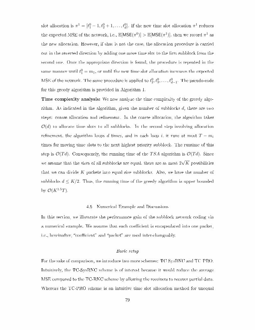
slot allocation is π1 = [t01 − 1, t02 + 1, . . . , t0d]. If the new time slot allocation π1 reduces
the expected MSE of the network, i.e., E[MSE(π0)] > E[MSE(π1)], then we record π1 as
the new allocation. However, if that is not the case, the allocation procedure is carried
out in the reversed direction by adding one more time slot to the �rst subblock from the
second one. Once the appropriate direction is found, the procedure is repeated in the
same manner until t01 = m1, or until the new time slot allocation increases the expected
MSE of the network. The same procedure is applied to t02, t03, . . . , t
0d−1. The pseudo-code
for this greedy algorithm is provided in Algorithm 1.
Time complexity analysis: We now analyze the time complexity of the greedy algo-
rithm. As indicated in the algorithm, given the number of subblocks d, there are two
steps: coarse allocation and re�nement. In the coarse allocation, the algorithm takes
O(d) to allocate time slots to all subblocks. In the second step involving allocation
re�nement, the algorithm loops d times, and in each loop i, it runs at most T − mi
times for moving time slots to the next highest priority subblock. The runtime of this
step is O(Td). Consequently, the running time of the TSA algorithm is O(Td). Since
we assume that the sizes of all subblocks are equal, there are at most 2√K possibilities
that we can divide K packets into equal size subblocks. Also, we have the number of
subblocks d ≤ K/2. Thus, the running time of the greedy algorithm is upper bounded
by O(K1.5T ).
4.5 Numerical Example and Discussions
In this section, we illustrate the performance gain of the subblock network coding via
a numerical example. We assume that each coe�cient is encapsulated into one packet,
i.e., hereinafter, �coe�cient� and �packet� are used inter-changeably.
Basic setup
For the sake of comparison, we introduce two more schemes: TC-SysRNC and TC-PRO.
Intuitively, the TC-SysRNC scheme is of interest because it would reduce the average
MSE compared to the TC-RNC scheme by allowing the receivers to recover partial data.
Whereas the TC-PRO scheme is an intuitive time slot allocation method for unequal
79

priority data. The transmission protocols of these two new schemes are described as
follows.
• Transmission of coe�cients with systematic random network coding (TC-SysRNC):
In this scheme, the transmission is divided into two phases: the basic phase and
the augmentation phase. In the basic phase, allK original packets are transmitted.
Next, in the augmentation phase, the sender transmits the coded packets generated
as in the TC-RNC scheme. The receivers, which might have lost some original
packets, can receive more coded packets to recover their own data by solving the
system of linear equations [76]. Note that, because packets are not mixed in the
basic phase, a receiver is able to obtain partial of the data, even if it cannot recover
all the mixed packets in the augmentation phase.
• Transmission of coe�cients with proportional time slot allocation (TC-PRO): In
this scheme, each of the K coe�cients is allocated time slots, proportional to its
weight. For example, let |θi| be the weight of coe�cient θi. Then the number of
time slots allocated to θi is ti = ⌊T |θi|/∑
j |θj |⌋. This allocation procedure starts
from the largest weight coe�cient to the smallest weight coe�cient, or stops when
there is no available time slot. The coe�cients are transmitted repeatedly in their
allocated time slots. This transmission scheme coarsely exploits the structure of
the power-law decay signal.
Before delving into the details, we should note that the TCM scheme requires more
bandwidth (by a factor of O(logN)) compared to the schemes that transmit coe�-
cients. Clearly, this is an unfair comparison since the two transmission strategies cater
to di�erent scenarios, as discussed before. In particular, the TCM scheme is used in
scenarios where the sender has limited resources. In contrast, the schemes that trans-
mit coe�cients are applied when the sender is more sophisticated. In this section, we
evaluate and compare the performances of the schemes that transmit coe�cients only.
In our example, we compare the proposed subblock network coding schemes with
TC-RR, TC-RNC, TC-SysRNC, and TC-PRO, in terms of outage probability and the
average MSE. We consider the multicast of a power-law decay signal of length N = 1000
80
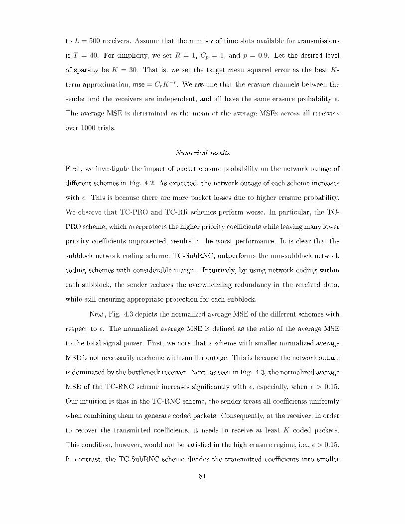
to L = 500 receivers. Assume that the number of time slots available for transmissions
is T = 40. For simplicity, we set R = 1, Cp = 1, and p = 0.9. Let the desired level
of sparsity be K = 30. That is, we set the target mean squared error as the best K-
term approximation, mse = CrK−r. We assume that the erasure channels between the
sender and the receivers are independent, and all have the same erasure probability ϵ.
The average MSE is determined as the mean of the average MSEs across all receivers
over 1000 trials.
Numerical results
First, we investigate the impact of packet erasure probability on the network outage of
di�erent schemes in Fig. 4.2. As expected, the network outage of each scheme increases
with ϵ. This is because there are more packet losses due to higher erasure probability.
We observe that TC-PRO and TC-RR schemes perform worse. In particular, the TC-
PRO scheme, which overprotects the higher priority coe�cients while leaving many lower
priority coe�cients unprotected, results in the worst performance. It is clear that the
subblock network coding scheme, TC-SubRNC, outperforms the non-subblock network
coding schemes with considerable margin. Intuitively, by using network coding within
each subblock, the sender reduces the overwhelming redundancy in the received data,
while still ensuring appropriate protection for each subblock.
Next, Fig. 4.3 depicts the normalized average MSE of the di�erent schemes with
respect to ϵ. The normalized average MSE is de�ned as the ratio of the average MSE
to the total signal power. First, we note that a scheme with smaller normalized average
MSE is not necessarily a scheme with smaller outage. This is because the network outage
is dominated by the bottleneck receiver. Next, as seen in Fig. 4.3, the normalized average
MSE of the TC-RNC scheme increases signi�cantly with ϵ, especially, when ϵ > 0.15.
Our intuition is that in the TC-RNC scheme, the sender treats all coe�cients uniformly
when combining them to generate coded packets. Consequently, at the receiver, in order
to recover the transmitted coe�cients, it needs to receive at least K coded packets.
This condition, however, would not be satis�ed in the high-erasure regime, i.e., ϵ > 0.15.
In contrast, the TC-SubRNC scheme divides the transmitted coe�cients into smaller
81

subblocks and appropriately allots time slots to each subblock. As a result, the larger
weight coe�cients would be received successfully with higher probability, leading to only
a slight increase in the average MSE.
0 0.05 0.1 0.15 0.20
0.1
0.2
0.3
0.4
0.5
0.6
0.7
0.8
0.9
1
Packet Erasure Probability
Out
age
Pro
babi
lity
Sparsity K = 30
TC−RR
TC−RNC
TC−SysRNC
TC−PRO
TC−SubRNC
Figure 4.2: P ∗out vs. ϵ.
0 0.05 0.1 0.15 0.20
0.01
0.02
0.03
0.04
0.05
0.06
Packet Erasure Probability
Nor
mal
ized
Ave
rage
MS
E
Sparsity K = 30
TC−RR
TC−RNC
TC−SysRNC
TC−PRO
TC−SubRNC
Figure 4.3: Normalized Avg. MSE vs. ϵ.
4.6 Conclusions
In this chapter, we considered transmission scenarios in which the sender multicasts a
compressively sampled signal to many receivers over lossy wireless channels. First, using
extreme value theory, we quanti�ed the network outage for both cases where the trans-
mitter may or may not be capable of reconstructing the compressively sampled signals.
We showed that when the sender can reconstruct the compressively sampled signals, the
strategy of using network coding to multicast the reconstructed signal coe�cients can
reduce the network outage signi�cantly. Next, we showed that the traditional network
coding could result in suboptimal performance with the power-law decay signals. With
this insight, we devised a new method, namely subblock network coding, which involves
fragmenting the data into subblocks, and allocating time slots to di�erent subblocks,
based on their priorities. We formulated the corresponding optimal allocation as an
integer programming problem, and developed a heuristic algorithm that exploits the
inherent priority structure of the power-law signals. We showed that by using subblock
network coding one can gain substantially in terms of network outage compared with
the other schemes. We are currently exploring the Markov Chain Monte Carlo method
82

to quantify the potential gain of subblock network coding.
To the best of our knowledge, there has been little work on multicasting com-
pressible signals, and this study here presents some initial steps to understand the in-
terplay between compressive sensing and network coding.
83

Chapter 5
DIGITAL RELAYING VERSUS ANALOG RELAYING: A SUFFICIENT
CONDITION FOR OPTIMALITY
5.1 Introduction
Recently, wireless sensor networks (WSNs) have attracted much attention of the research
community. Due to their high �exibility, enhanced surveillance coverage, robustness,
mobility, and cost e�ectiveness, WSNs have wide applications and high potential in
military surveillance, security, monitoring of tra�c, and environment. Usually, a WSN
consists of a large number of low-cost and low-power sensors, which are deployed in the
environment to collect observations and preprocess the observations. Each sensor node
has limited communication capability that allows it to communicate with other sensor
nodes via a wireless channel. Often, there is a fusion center that processes data from
sensors and forms a global situational assessment.
The ability to detect events of interest is a key capability of the sensor network
technology. Detection is the �kick-start� procedure for the operation of any sensor net-
work. Indeed, the physical attributes of a target, like its position and velocity, can be
ascertained only after having detected its presence. Furthermore, in some applications
such as surveillance, industrial monitoring etc., the detection of an intruder or a hazard
is the prime goal.
The decision-making problem, where each sensor sends to the fusion center a
summary of its own observations, in the form of a message taking values from a �nite
alphabet, is termed decentralized detection. Decentralized detection scenarios for sensor
networks typically entail geographically dispersed sensors that collect observations about
an �event� of interest and transmit information about these individual observations to a
fusion center. The fusion center produces an estimate about the event, based on the data
it receives from the sensors. If the event is binary with a known prior probability distri-
bution, the problem falls into the Bayesian detection framework, and the probability of
error at the fusion center is a typical metric of performance. When no prior distribution
on the event is available, Neyman-Pearson detection seeks to minimize the probability
84

of false alarm subject to a constraint on the probability of missed detection [78]. A key
challenge in decentralized detection is to come up with decision rules at the sensors,
and fusion rules at the fusion center so as to optimize the detection performance at the
fusion center.
Wireless sensor nodes are typically tiny devices powered by batteries, and hence
are subject to stringent constraints on the resources such as, bandwidth and power. To
design an e�cient system for detection in sensor networks, it is imperative to understand
the interplay between data processing at the sensor nodes, resource allocation, and over-
all performance in distributed sensor systems. A clear understanding of this interplay
can be leveraged to gain insight into the e�cient design of sensor networks. Decentral-
ized detection has received much attention in the literature due to its importance in the
event driven sensor networks. In-depth treatments of this �eld can be found in the work
of Tsitsiklis [79], Viswanathan et al. [80] and Blum et al. [81], and the references therein.
A recent survey on channel-aware distributed detection, where sensors communicate to
the fusion center over noisy (and fading) links, can be found in [82].
Early treatments of distributed detection adopted various simplifying assump-
tions, particularly about independence of observations at the sensors, and about com-
munication between the sensor nodes and the fusion center, which was often assumed
to be perfect. When these assumptions hold, the performance of a decentralized system
is optimized by each sensor transmitting its likelihood ratio to the fusion center. The
fusion center forms a global likelihood ratio from the product of these and achieves per-
formance equivalent to what would be possible if all the raw sensor data were available
at the fusion center. If the communication links between the sensors and the fusion cen-
ter are imperfect, performance may actually be improved by quantizing the individual
sensor likelihood ratios prior to transmission to the fusion center. Some observations
along this line have been made by other authors in various contexts. In [83], for example,
it is observed that analog sensors perform better than their digital counterpart below
a certain threshold SNR in large sensor networks where the metric of performance is
the Cherno� exponent. In [84], a distributed detection method based on the method
of types is considered. Again in this setting, it is observed that hard-decision fusion
85

Event Relay Sensor Fusion Center
Figure 5.1: Block diagram of a typical sensor relay network.
(digital relaying) can outperform soft-decision fusion (analog relaying) in the single sen-
sor case. In this chapter, comparison of analog and digital relay schemes is undertaken
from a classical decision theoretic perspective for a simple network model consisting of
a single sensor communicating with the fusion center over an additive Gaussian noise
channel. A Bayesian situation is assumed and probability of error at the fusion center is
the performance metric. In this setting, a su�cient condition for superiority of digital
relaying, given a �xed average transmit power, is derived analytically in terms of the
observation SNR at the sensor and the SNR of the communication channel between the
sensor node and the fusion center.
Although the network model used here is highly simpli�ed, it is hoped that this
work will contribute to a foundation for analysis of more realistic scenarios, leading to
advances in sensor placement strategies and inference algorithms in sensor networks as
well as the design of wireless relay networks [85] in which a relay assists communication
between a source-destination pair.
The rest of this chapter is organized is as follows. Section 5.2 presents the system
model and assumptions. Section 5.3 introduces the relaying methods and presents the
mathematical framework. Section 5.4 compares the performance of relaying schemes.
Section 5.5 discusses simulation results, and some concluding remarks are given in Sec-
tion 5.6.
5.2 System Model
We consider a single sensory relay network, consisting of a relay-sensor and fusion center,
with a power constraint at the relay. The system is as shown in the Fig. 5.1. The prime
86

objective of the network is to make a decision on a binary event at the fusion center with
minimum detection error. The job of relay sensor is to assist the fusion center in making
a decision on the event. We assume that the underlying phenomenon is an equally-likely
binary event, S ∈ {0, 1}. In terms of null-hypothesis (H0) and target-hypothesis (H1),
we write
H0 : S = 0, P (H0) = 0.5
H1 : S = 1, P (H1) = 0.5.
The sensor observes a noisy stochastic process Xn associated with the event. We
represent the observation process at the sensor as
Xn = hSn + Zn, n = 1, . . . , (5.1)
where h represents the scaling factor accounting for the uncertainties in the amplitude
of the event sensed by the sensor, and Zn is an i.i.d additive Gaussian process with
Zn ∼ N (0, σ2z). We assume that the sensor has knowledge of h, and hence, the sensor
observations are independent conditioned on the hypothesis (Sn) and h. Upon observing,
the sensor processes Xn to obtain a statistic Un, which is relayed to the fusion center,
adhering to an average transmit power constraint of P . The local processing rule for
the observations at the sensor node, denoted by γ, is de�ned as
γ : X → U , (5.2)
where X is the observation space and U denotes the output space of the sensor. Due
to the transmit power constraint P at the sensor, it is clear that E[|U |2] ≤ P , for all
U ∈ U . Observe that the processing rule at the sensor node, γ, depends on the relaying
scheme.
The relay sensor, after computing a statistic Un from its observations, transmits
Un to the fusion center over a wireless link for decision making. We assume that fusion
center has no access to the observations of the event, and has to make a decision solely
based on the information sent from the relay. We represent the signal received by the
fusion center as
Yn = gUn +Wn, n = 1, . . . , (5.3)87

where g represents channel attenuation, and Wn is an i.i.d. additive Gaussian process
with Wn ∼ N (0, σ2w). We assume that the fusion center is cognizant of its channel state
g, and hence the observations are conditionally independent given g and the hypothesis.
The fusion center has to make a decision Sn based on the information relayed by the
sensor. The objective is to minimize the detection error under the transmit power
constraint at the relay. In what follows, we formulate and analyze the problem in hand
under classical binary hypothesis testing framework, and develop a fair idea about the
relaying schemes. We assume that the detection is performed on a sample-by-sample
basis. In what follows, for presentational convenience, we omit the use of temporal
subscript n.
5.3 Relaying Schemes
Upon obtaining the noisy observations of the event, the sensor is posed with the problem
of computing a statistic (that is, to design γ) so as to aid fusion center in decision making.
The senors can be �digital� or �analog� depending on the processing schemes. A digital
sensor may quantize its observations and communicate its decisions in the form of bits,
while an analog sensor may compute the su�cient statistics of its observations, which is
a real number, and may transmit it as an analog signal. Assessing the performances of
these schemes in di�erent regimes of network parameters is key to the design of sensor
and relay networks. One wishes to deploy analog or digital sensors depending on which
scheme is superior in a given regime.
Digital relaying (detect and forward)
The relay sensor performs binary hypothesis testing on the observations and the decision
is conveyed in the form of a bit. Thus, the decision variable U is binary. That is, with
the power constraint, U ∈ {−√P,√P}. We express the likelihood function at the sensor
as
H0 : X ∼ fX(zi|H0, h),
H1 : X ∼ fX(zi|H1, h).
88

where
fX(x|H0, h) =1√2πσ2z
exp− x2
2σ2z;
fX(x|H1, h) =1√2πσ2z
exp−(x− h)2
2σ2z.
From the fundamentals of detection theory [78], it is clear that the optimal processing
rule is given by
U = γ(X) =
+√P if fX(x|H1, h) ≥ fX(x|H0, h)
−√P if fX(x|H1, h) < fX(x|H0, h).
(5.4)
More succinctly, we have the sensor's processing rule as
γ(X) =√P [2I(X ≥ h/2)− 1] , (5.5)
where I(·) is the indicator function.
Next, consider the fusion rule at the fusion center. The fusion center receives
Y , a noisy version of the statistic U communicated by sensor over the noisy link. It
is faced with the task of making decision S, on S, based on the received signal Y .
Observe that the distribution of Y , and therefore the fusion rule, depend on the decision
rule γ, of the sensor. Therefore, to derive the decision rule at the fusion center, it is
essential �rst to evaluate the detection error probabilities at the sensor. To this end, we
de�ne SNRo∆= 1
4h2
σ2z, as the observation SNR, which is the �signal-to-noise ratio� of the
observations at the sensor. Then, for a given SNRo, we note that the probability of error
at the sensor, p, is given by:
p = P (X ≥ h/2|S = 0, SNRo) = Q(√
SNRo
), (5.6)
where Q(·) is the Q−function given by Q(x) = 1√2π
∫ x0 e
−u2
2 du.We note that the received
signal Y obeys:
H0 : Y = −√Pg +W w.p. 1− p
Y =√Pg +W w.p. p
H1 : Y =√Pg +W w.p. 1− p
Y = −√Pg +W w.p. p.89

Particularly, Y is conditionally distributed as a mixture-Gaussian distribution given by
H0 : fY (y|H0, g) =1√2πσ2w
((1− p) exp−(y + g
√P )2
2σ2w+ p exp−(y − g
√P )2
2σ2w
)(5.7)
H1 : fY (y|H1, g) =1√2πσ2w
((1− p) exp−(y − g
√P )2
2σ2w+ p exp−(y + g
√P )2
2σ2w
).
We point out that, in reality, the optimal detection strategy involves coupling
between the decision procedures at the sensor and the fusion center. However, the
evaluation of thresholds and the analysis of the optimal scheme is intractable in general.
Therefore, in the developments of this section, we adapt the so-called �person-by-person
optimization" approach (PBPO) [79], where the decision at the fusion center is optimized
assuming �xed decision rules at the sensor.
Therefore, following PBPO approach, the decision process at the fusion center
boils down to classical hypothesis testing with
Choose S = 1, if L(Y ) ≥ 1,
where L(y) is the likelihood ratio, given by
L(y) =p exp−(2g
√Py
σ2w
) + 1− p
(1− p) exp−(2g√Py
σ2w
) + p. (5.8)
After some steps, the decision rule simpli�es to
Choose S = 1 if gY ≥ 0.
Next, we evaluate the detection error due to this �digital relaying� scheme. We
let SNRl∆= g2P/σ2w denote the link SNR, i.e., signal-to-noise ratio of the link between
sensor and the fusion center. For convenience, de�ne SNR = [SNRo, SNRl]. The detection
error at the fusion center, when aided by a digital sensor, is given by
PED(SNR) = p+ (1− 2p)Q(√
SNRl
), (5.9)
where p is given by the equation (5.6).
90

Analog relaying (estimate and forward)
This case employs analog sensor to aid fusion center. Relay sensor constructs a su�cient
statistic of the phenomenon, scales the message for the given power constraint and
transmits it to the sink. Essentially, the sensor node acts as an analog relay ampli�er
with the output space, U = R with E[|U |2] ≤ P for all U ∈ U . It is clear that the
su�cient statistic T is given by the log likelihood ratio,
T (x) = logfX(x|H1, h)
fX(x|H0, h)=
h
2σ2z(2x− h) . (5.10)
It follows that T is a Gaussian RV with variance Var(T ) = 4SNRo, and E[T |H0] = −2SNRo
and E[Ti|H1] = 2SNRo.
Accounting for the average power constraint, the message sent from the relay is
given by
U(X) =
√P
4SNRo(1 + SNRo)T (X) (5.11)
so that
H0 : U ∼ N
(−√
PSNRo1 + SNRo
,P
1 + SNRo
)
H1 : U ∼ N
(√PSNRo1 + SNRo
,P
1 + SNRo
).
The fusion center receives Y , a noisy version of U , and performs decision on the event
based on Y , so as to minimize the probability of detection error. The decision rule at
the fusion center is the likelihood ratio test, given as:
Choose S = 1, iffY (y|H1, g)
fY (y|H0, g)≥ 1.
We note that
H0 : Y ∼ N
−√g2PSNRo1 + SNRo
, g2P
1 + SNRo+ σ2w
H1 : Y ∼ N
√g2PSNRo1 + SNRo
, g2P
1 + SNRo+ σ2w
.
It follows that the optimal rule simpli�es to
Choose S = 1 if gY ≥ 0.91

Consequently, for a given set of SNR parameters, SNR, the detection error at the fusion
center when aided by an analog sensor can be shown to be
PEA(SNR) = Q
(√SNRlSNRo
SNRl + SNRo + 1
). (5.12)
5.4 Comparison of Analog and Digital Relaying
In this section, we compare the performance of analog and digital relaying schemes just
described, in terms of observation and link SNRs. It is unclear, a priori, in which regimes
one scheme outperforms the other. We partly answer the above question by providing a
su�cient condition for the optimality of digital scheme over the analog scheme. Before
presenting our main result, we state the following lemma.
Lemma 5.1. Let a, b ≥ 0 such that a+ b ≤ 12 , then
Q
(1√a+ b
)≥ Q
(1√a
)+Q
(1√b
).
Proof. Let a ≥ b, so that 1√a+b≤ 1√
a≤ 1√
b. We have
Q
(1√a+ b
)−
[Q
(1√a
)+Q
(1√b
)]=
1√2π
∫ 1√a
1√a+b
e−x2
2 dx− 1√2π
∫ ∞
1√b
e−y2
2 dy
≥ 1√2π
∫ 1√a
1√a+b
√axe−
x2
2 dx− 1√2π
∫ ∞
1√b
√bye−
y2
2 dy
=e− 1
2(a+b)
√2π
[√a−
(√a e
− b2a(a+b) +
√b e
− a2b(a+b)
)]≥ e
− 12(a+b)
√2π
[√a−
(√a e−
ba +√b e−
ab
)]≥ e
− 12(a+b)
√2π
√a[1−
(e−
ba + e−
ab
)]≥ 0,
where the �rst inequality follows from the fact that x ≤ 1√afor the �rst integral and
y ≥ 1√bfor the second integral. Second inequality follows from the assumption that
a + b ≤ 12 , third inequality is by a ≥ b, and the last inequality is due to fact that(
e−x + e−1x
)≤ 1 for x ≥ 0.
92

The following result establishes that for the values of SNRs beyond a certain
threshold, digital relaying is superior to analog relaying.
Proposition 5.1. [Optimality of Digital Relaying]: For all observation and link
SNRs, SNR = [SNRo, SNRl] such that 1/SNRo + 1/SNRl ≤ 1/2, it is optimal to use digital
relaying over analog relaying, i.e., PED(SNR) ≤ PEA(SNR).
Proof. From (5.9) and (5.12), and using the fact that Q(·) is a decreasing function of
its argument, it is clear that
PED(SNR) ≤ Q(√
SNRo
)+Q
(√SNRl
)(5.13)
and
PEA(SNR) ≥ Q(√
SNRlSNRo
SNRl + SNRo
). (5.14)
Setting a = 1SNRo
and b = 1SNRl
, and applying Lemma 5.1, we obtain
PEA(SNR)− PED(SNR) ≥ Q
(1√a+ b
)−[Q
(1√a
)+Q
(1√b
)]≥ 0.
Proposition 5.1 asserts that for the single sensor case, under the regime of mod-
erately high observation and link SNRs, the digital scheme performs better than the
analog scheme. This behavior can be explained intuitively as follows. Under digital
scheme, since only the decision bits are communicated, sensor just acts as a ampli�er-
repeater on the event and hence the power spent per symbol is more, which, in turn,
manifests the distortions su�ered by the signal over the forward link. In case of analog
scheme, the su�cient statistic, which is a real number, is communicated and the power
spent on the symbol is insu�cient to overcome the deleterious e�ects of the channel.
Thus, when the SNR either at the backward link or at the forward link grows large,
analog and digital schemes become equivalent.
5.5 Simulation Results
In this section, we evaluate the performance of digital and analog schemes. The per-
formance metric is the decision error as a function of link SNR, for a �xed observation93

SNR. Fig. 5.2 shows the performance curves as a function of SNRl, for an observation
SNR of 3dB. It can be seen that the digital scheme clearly outperforms analog scheme.
As SNRl increases, the di�erence in the performance diminishes due to the fact that
limSNRl→∞
PED(SNR) = limSNRl→∞
PEA(SNR) = Q(√SNRo). (5.15)
−10 −5 0 5 10 15 20 25 300.05
0.1
0.15
0.2
0.25
0.3
0.35
0.4
Link SNR, SNRl (dB) ®
Pro
babi
lity
of D
etec
tion
Err
or P
e ®
P
ED simulated
PED
theoretical
PEA
simulated
PEA
theoretical
Figure 5.2: Pe vs. SNRl for SNRo = 3 dB.
−10 −5 0 50.24
0.26
0.28
0.3
0.32
0.34
0.36
0.38
0.4
0.42
Link SNR, SNRl (dB)
PR
obab
ility
of D
etec
tion
Err
or P
e
P
ED simulated
PED
theoretical
PEA
simulated
PEA
theoretical
PEA
< PED P
ED < P
EA
Figure 5.3: Pe vs. SNRl for SNRo = −3 dB.
5.6 Conclusions
In this work, we considered the problem binary hypothesis testing in a single sensory
relay network. In particular, we studied and compared two schemes, namely: detect-and-
forward (digital relaying) and estimate-and-forward (analog relaying). We observed that
the performance of relaying scheme depends on observation as well as link SNRs. We
established a su�cient condition for the optimality digital relaying over analog relaying.
This can have important implications on the design of sensor and communication relay
networks. As a part of the future work, we wish to address the necessary condition
for the optimality of digital sensors. Furthermore, the developments in the paper are
carried under a classical hypothesis testing framework. It will be interesting to carry
out a similar analysis and comparison with respect to di�erent classes detectors like
NP-detector, min-max detector etc.
94

Chapter 6
CONCLUSIONS AND DISCUSSIONS
In this thesis, we have laid out a framework to build a clear understanding of the value
of information in wireless networks. The scope of information in this thesis is broad,
ranging from channel/network states to the structure of the signal itself. Under the
common thread of characterizing the value of information, we have investigated three
important scenarios of wireless networks, namely opportunistic scheduling, cooperative
relaying and multicasting in wireless networks. In the case of opportunistic scheduling,
the information was in form of channel state information; in the case of cooperative re-
laying, it was in the form of partial knowledge of the concurrent interfering message; and
in the multicasting scenario, information was the knowledge about the physical nature
of the signal itself. Exploiting the available information to devise adaptive strategies is
a key ingredient in these studies. Through rigorous analysis and numerical examples,
we demonstrated that, by suitably exploiting the available information, one can gain
substantially in terms of system performance. In what follows, we brie�y outline our
key contributions with discussions, and possible future directions.
6.1 Distributed Opportunistic Scheduling
Channel-aware scheduling is a promising technique to harness the rich diversities inher-
ent in wireless networks. In channel-aware scheduling, a joint physical layer (PHY)/medium
access control (MAC) optimization is utilized to improve network throughput by schedul-
ing links with good channel conditions for data transmissions. However, to reap rich
dividends from channel-aware scheduling, one has to carefully understand these dynam-
ics of PHY/MAC diversities. Therefore, in this context, the availability of information
at the participating nodes, about the PHY/MAC dynamics, becomes critical. In ad-hoc
networks where there is no centralized decision maker, making this information available
becomes more challenging. We addressed this challenge by considering a framework for
distributed opportunistic scheduling (DOS).
DOS involves a process of joint channel probing and distributed scheduling
for ad-hoc (peer-to-peer) communications. The objective is to maximize the system
95

throughput. While related works in DOS hinge on the assumption of perfect channel
state information (CSI), in practice, the CSI is often imperfect due to noisy estimation.
When the CSI is imperfect, the transmission rate has to be backed o� from the esti-
mated rate to avoid transmission outages. This may result in throughput degradation,
which is proportional to the estimation error. Clearly, a plausible solution to enhance
the throughput is to mitigate the rate estimation errors by performing further channel
probing.
With this motivation, our DOS framework is centered around cleverly tackling
incomplete channel information, with the option of re�ning the CSI for the scheduled
user. However, the advantages of second-level probing come at the price of additional
overhead. Thus, there is a tradeo� between the throughput gain from better channel
conditions and the cost for further probing. We showed that this tradeo� reduces to
judiciously choosing an optimal stopping rule for channel probing and the transmission
rate for throughput maximization. Capitalizing on optimal stopping theory with in-
complete information, we showed that the optimal scheduling policy is threshold-based,
and is characterized by either one or two thresholds, depending on network settings.
We rigorously established necessary and su�cient conditions for both cases. In par-
ticular, we observed that performing second-level channel probing is optimal when the
�rst-level estimated channel condition falls in between the two thresholds. Numerical
results illustrate the e�ectiveness of the proposed DOS with two-level channel probing.
We also extended our study to the case with limited feedback, where the feedback from
the receiver to its transmitter takes the form of (0, 1, e). We note that the proposed
distributed scheduling with two-level probing provides a new framework to study joint
PHY/MAC optimization in practical networks where noisy probing is often the case
and imperfect information is inevitable. We believe that this line of study provides
some initial steps towards opening a new avenue for exploring the intrinsic tradeo�s
between probing (sensing) and scheduling to enhance spectrum utilization; and this is
potentially useful for enhancing MAC protocols for wireless mesh networks and cognitive
radio networks.
In this work, we have considered DOS with two-level probing, where it is assumed
96

that the re�nement of the rate estimate is carried out once, via second-level probing
of duration τ . However, we can further extend this to L−level probing, where for
k = 1, . . . , L − 1, a successfully contending transmitter has the options 1) to transmit,
or 2) to defer and re-contend, or 3) to resort to (k + 1)−st level training at the cost
of additional overhead. In this situation, it is of interest to devise well-structured, yet
simple policies. Extending the current results on single-hop ad hoc networks to multi-
hop models is also of considerable interest for future study.
6.2 Cooperative Relaying
It is well-known that interference is a detrimental phenomenon in wireless communica-
tion, limiting the system performance. Interference management is a key issue in the
design of wireless systems. Most state-of-the-art wireless systems deal with interference
in one of two ways: To orthogonalize the communication links in time or frequency, so
that they do not interfere with each other at all; or, to allow the communication links to
share the same degrees of freedom, but treat each other's interference as adding to the
noise �oor. It is clear that both approaches can be sub-optimal. The �rst approach en-
tails an a priori loss of degrees of freedom in both links, no matter how weak the potential
interference is. The second approach treats interference as pure noise while it actually
carries information and has structure that can potentially be exploited in mitigating its
e�ect. These treatments are based on the assumption that the each transmitter/receiver
pair is isolated from other. In various practical scenarios, however, they are not isolated,
and cooperation among transmitters or receivers can be induced. Further, other nodes
in the network can serve as relays, and cooperate with the active links in mitigating the
interference. A key outcome of this view is that, due to the broadcast nature of the
wireless medium, each node in the network obtains partial side information about the
interference. The main challenge then is exploit this side information to improve the
system performance.
With this motivation, we considered a two-hop interference network in which
two sources wish to communicate simultaneously with two destinations, and are aided
by two relay nodes. The transmissions interfere with each other in each hop. A key
97

observation is that, while the transmission during the �rst hop is essentially over a
classical interference channel, the transmission in the second hop enjoys an interesting
advantage. Speci�cally, the second hop represents an interference channel with partial
side-information at the transmitters. Consequently, this opens the door to cooperation
between the relays. In light of this, we proposed various cooperative relaying strategies
based on distributed MIMO broadcast, to enhance the achievable rate of the information
�ows. Indeed, we observed that, by exploiting the side information available at the
transmitters, the proposed strategies gain substantially over other strategies considered
in the literature.
Next, we discuss some possible future extensions. In this work, we have con-
sidered a two-hop model comprising two information �ows. It will be interesting to
consider more than two �ows (i.e., more than two source-destination pairs aided by re-
lays) in a two-hop network. Further, throughout this study, we have assumed that all
nodes the network have perfect knowledge of their direct and interfering link conditions.
An interesting direction would be to relax the assumption of perfect state information
and study its impact on the throughput of the network. Also, it will be interesting
to consider the more realistic case where the transmitter nodes have no channel state
information. In this case, possible transmission strategies could involve cooperation as
well as competition.
6.3 Digital versus Analog Relaying
We considered a basic scenario in sensor networks, where a single sensor node relays
a statistic of its observations of an event to the fusion center which performs the �nal
inference on the event. We considered two relaying schemes: analog relaying and digital
relaying. With ultimate detection error at the fusion center being the performance
metric, we provided su�cient conditions for the optimality of analog relaying over digital
relaying in this network. This observation has potential applications in the design and
placement of sensor nodes in sensor networks.
There are several directions for extending this work. In this work, we have
given only a su�cient condition for the optimality of digital relaying. However, one
98

can strengthen this result by establishing the necessary conditions. Furthermore, the
developments in this work are carried under a classical hypothesis testing framework.
It will be interesting to carry out a similar analysis and comparison with respect to
di�erent classes detectors like NP-detector, min-max detector etc.
6.4 Multicasting
To understand the value of information in the multicast scenario, we considered multicas-
ting compressively sampled signals from a source to many receivers, over lossy wireless
channels. We focused on the network outage from the perspective of signal distortion
across all receivers, for both cases where the transmitter may or may not be capable
of reconstructing the compressively sampled signals. Based on extreme value theory,
we characterized the network outage in terms of key system parameters, including the
erasure probability, the number of receivers and the sparse structure of the signal. When
the transmitter can reconstruct the compressively sensed signal, the strategy of using
network coding to multicast the reconstructed signal coe�cients can reduce the network
outage signi�cantly. However, the traditional network coding could result in suboptimal
performance for power-law decay signals. Thus motivated, we devised a new method,
using subblock network coding, which involves fragmenting the data into subblocks, and
allocating time slots to di�erent subblocks, based on their priorities. The correspond-
ing optimal allocation is formulated as an integer programming problem. Since integer
programming is often intractable, we developed a heuristic algorithm that prioritizes
the time slot allocation by exploiting the inherent priority structure of power-law de-
cay signals. Through numerical results, we demonstrated that the proposed schemes
outperform the traditional methods with signi�cant margins.
As a part of the future work, we are currently exploring the Markov Chain Monte
Carlo method to quantify the potential gain of subblock network coding. In this work,
we have considered a centralized scheme for compressing/sampling the information. A
potentially explorable direction would be to look into distributed ways of exploiting the
structure of the signals in sampling and compressing them. This can have signi�cant
implications in reducing transmission and processing burdens in sensor networks.
99

REFERENCES
[1] D. Aguayo, J. Bicket, S. Biswas, G. Judd, and R. Morris, �Link-level measurements
from an 802.11b mesh network,� in In SIGCOMM, 2004, pp. 121�132.
[2] M. Cao, V. Raghunathan, and P. Kumar, �Cross-layer exploitation of MAC layer
diversity in wireless networks,� in Proc. ICNP '06, USA, 2006, pp. 332�341.
[3] M. Andrews, K. Kumaran, K. Ramannan, A. Stolyar, R. Vijaykumar, and P. Whit-
ing, �CDMA data QoS scheduling on the forward link with variable channel condi-
tions,� Bell Labs Tech. Memo., April 2000.
[4] S. Borst, �User-level performance of channel-aware scheduling algorithms in wireless
data networks,� in Proc. IEEE INFOCOM'03, San Francisco, CA, 2003.
[5] R. Knopp and P. A. Humblet, �Information capacity and power control in single-cell
multiuser communications,� in Proc. IEEE ICC'95, vol. 1, USA, 1995, pp. 331�335.
[6] P. Viswanath, D. N. C. Tse, and R. Laroia, �Opportunistic beamforming using dumb
antennas,� IEEE Trans. Inf. Theory, vol. 48, no. 6, pp. 1277�1294, Jun. 2002.
[7] D. Zheng, W. Ge, and J. Zhang, �Distributed opportunistic scheduling for ad-hoc
communications: An optimal stopping approach,� in Proc. Mobihoc 2007, Montreal,
Canada, Sept. 2007.
[8] D. Zheng, M. O. Pun, W. Ge, J. Zhang, and H. V. Poor, �Distributed opportunistic
scheduling for ad hoc communications with imperfect channel information,� IEEE
Trans. Wireless Commun., vol. 7, pp. 5450�5460, Dec. 2008.
[9] A. Vakili, M. Sharif, and B. Hassibi, �The e�ect of channel estimation error on the
throughput of broadcast channels,� in Proc. of IEEE Int. Conf. Acoustics, Speech,
and Signal Processing (ICASSP'06), Toulouse, France, May 2006.
100

[10] W. Stadje, �An optimal stopping problem with two levels of incomplete informa-
tion,� Mathematical Methods of Operations Research, vol. 45, no. 1, pp. 119�131,
1997.
[11] D. Assaf, L. Goldstein, and E. Samuel-Cahn, �A statistical version of prophet in-
equalities,� Annals of Statistics, vol. 26, pp. 1190�1197, 1996.
[12] M. H. M. Costa and A. A. E. Gamal, �The capacity region of the discrete memoryless
interference channe with strong interference (corresp.),� IEEE Trans. Info. Theory,
vol. 33, no. 5, Sept. 1987.
[13] T. Han and K. Kobayashi, �A new achievable rate region for the interference chan-
nel,� IEEE Trans. Info. Theory, vol. 27, no. 1, Jan 1981.
[14] R. H. Etkin, D. N. C. Tse, and H. Wang, �Gaussian Interference Channel Capacity
to Within One Bit,� IEEE Trans. Info. Theory, vol. 54, no. 12, pp. 5534�5562, 2008.
[15] E. C. van der Meulen, �A survey of multiway channels in information theory: 1961-
1976,� IEEE Trans. Info. Theory, vol. 23, no. 1, Jan. 1977.
[16] J. Laneman, D. Tse, and G. Wornell, �Cooperative diversity in wireless networks:
E�cient protocols and outage behavior,� IEEE Trans. Info. Theory, vol. 50, no. 12,
pp. 3062�3080, Dec. 2004.
[17] S. I. Gel�fand and M. S. Pinsker, �Coding for channel with random parameters,�
Problems in Control and Information Theory, vol. 9, no. 1, pp. 19�31, 1980.
[18] R. Ahlswede, N. Cai, R. Li, and R. W. Yeung, �Network information �ow,� IEEE
Trans. Info. Theory, vol. 46, pp. 1204�1216, July 2000.
[19] D. Donoho, �Compressed sensing,� IEEE Trans. Info. Theory, vol. 52, no. 4, pp.
1289 � 1306, 2006.101

[20] E. J. Candès and M. B. Wakin, �An introduction to compressive sampling,� IEEE
Signal Processing Magazine, vol. 25, no. 2, pp. 21�30, March 2008.
[21] E. J. Candès and T. Tao, �Near-optimal signal recovery from random projections:
Universal encoding strategies?� IEEE Trans. Info. Theory, vol. 52, no. 12, pp.
5406�5425, 2006.
[22] X. Qin and R. Berry, �Exploiting multiuser diversity for medium access control in
wireless networks,� in Proc. IEEE INFOCOM'03, San Francisco, CA, Apr. 2003.
[23] Z. Ji, Y. Yang, J. Zhou, M. Takai, and R. Bagrodia, �Exploiting medium access
diversity in rate adaptive wireless LANs,� in Proc. ACM/IEEE MOBICOM'04,
Philadelphia, PA, Sept. 2004.
[24] X. Liu, E. K. Chong, and N. B. Shro�, �A framework for opportunistic scheduling
in wireless networks,� Computer Networks, vol. 41, no. 4, pp. 451�474, Mar. 2003.
[25] D. Zheng, W. Ge, and J. Zhang, �Distributed opportunistic scheduling for ad hoc
networks with random access: An optimal stopping approach,� IEEE Trans. Inf.
Theory, vol. 55, no. 1, pp. 205�222, Jan. 2009.
[26] B. Wang, J. Zhang, and L. Zheng, �Achievable rates and scaling laws of power-
constrained wireless sensory relay networks,� IEEE Trans. Inf. Theory, vol. 52,
no. 9, pp. 4084�4104, Sept. 2006.
[27] Z. Ye, A. Abouzeid, and J. Ai, �Optimal stochastic policies for distributed data
aggregation in wireless sensor networks,� IEEE/ACM Trans. Netw., vol. 17, no. 5,
pp. 1494�1507, Oct. 2009.
[28] T. Ferguson, Optimal Stopping and Applications. Electronic text, available at
http://www.math.ucla.edu/~tom/Stopping/Contents.html, 2006.
102

[29] Y. S. Chow, H. Robbins, and D. Siegmund, Great Expectations: Theory of Optimal
Stopping. Houghton Mi�in, 1971.
[30] A. N. Shiryayev, Optimal Stopping Rules. New York, NY: Springer-Verlag, 1978.
[31] D. P. Bertsekas and R. Gallager, Data Networks. Upper Saddle River, NJ: Prentice-
Hall, 1992.
[32] W. Ge, J. Zhang, J. Wieselthier, and S. Shen, �PHY-aware distributed scheduling
for ad hoc communications with physical interference model,� IEEE Trans. Wireless
Commun., vol. 8, no. 5, pp. 2682 � 2693, May 2009.
[33] B. Sadeghi, V. Kanodia, A. Sabharwal, and E. Knightly, �Opportunistic media
access for multirate ad hoc networks,� in Proc. ACM/IEEE MOBICOM'02, Atlanta,
GA, 2002.
[34] S. M. Kay, Fundamentals of Statistical Signal Processing: Estimation Theory. En-
glewood Cli�s, NJ: Prentice-Hall, 1993.
[35] T. Kailath, A. Sayed, and B. Hassibi, Linear Estimation. Englewood Cli�s, NJ:
Prentice Hall, 2000.
[36] H. Jiang, L. Lai, R. Fan, and H. V. Poor, �Optimal selection of channel sensing order
in cognitive radio,� IEEE Trans. Wireless Commun., vol. 8, no. 1, pp. 297�307, Jan.
2009.
[37] R. Ahlswede, �The capacity region of a channel with two senders and two receivers,�
The Annals of Probability, vol. 2, no. 5, 1974.
[38] O. Simeone, O. Somekh, Y. Bar-Ness, H. V. Poor, and S. Shamai, �Capacity of
linear two-hop mesh networks with rate splitting, decode-and-forward relaying and
103

cooperation,� in Proc. 45th Annual Allerton Conference on Communication, Con-
trol, and Computing, 2007.
[39] O. Oyman and A. J. Paulraj, �Leverages of distributed MIMO relaying: A
Shannon-theoretic perspective,� in 1st IEEE Workshop on Wireless Mesh Networks
(WiMesh'05), 2005.
[40] S. Shamai and B. M. Zaidel, �Enhancing the cellular downlink capacity via co-
processing at the transmitting end,� in Proc. IEEE Vehicular Technology Conf.,
May 2001.
[41] K. Marton, �A coding theorem for the discrete memoryless broadcast channel,�
IEEE Trans. Info. Theory, vol. 25, no. 3, pp. 306 � 311, may. 1979.
[42] M. H. M. Costa, �Writing on dirty paper,� IEEE Trans. Info. Theory, vol. 29, no. 3,
May 1983.
[43] H. Weingarten, Y. Steinberg, and S. Shamai, �The capacity region of the Gaus-
sian multiple input multiple output broadcast channel,� IEEE Trans. Info. Theory,
vol. 52, no. 9, Sept. 2006.
[44] S. Mohajer, S. N. Diggavi, C. Fragouli, and D. N. C. Tse, �Approximate capacity
of Gaussian interference-relay networks with weak cross links,� CoRR, vol. Arxiv:
1005.0404, 2010.
[45] Y. Cao and B. Chen, �Capacity bounds for two-hop interference networks,� in 47th
Annual Allerton Conference on Communication, Control, and Computing, 2009,
Sep. 2009, pp. 272 �279.
[46] P. Thejaswi, A. Bennatan, J. Zhang, R. Calderbank, and D. Cochran, �Rate-
achievability strategies for two-hop interference �ows,� in 2008 46th Annual Aller-
104

ton Conference on Communication, Control, and Computing, Sep. 2008, pp. 1432
�1439.
[47] I. Maric, R. Yates, and G. Kramer, �Capacity of interference channels with partial
transmitter cooperation,� IEEE Trans. Info. Theory, vol. 53, no. 10, Oct. 2007.
[48] V. Prabhakaran and P. Viswanath, �Interference channels with source cooperation,�
Submitted to IEEE Trans. Info. Theory, 2010.
[49] I. Wang and D. N. C. Tse, �Interference Mitigation through Limited Transmitter
Cooperation,� ArXiv: 1004.5421, Apr. 2010.
[50] Y. Cao and B. Chen, �An achievable rate region for interference channels with
conferencing,� in IEEE International Symposium on Information Theory, 2007.
ISIT 2007., Jun. 2007, pp. 1251 �1255.
[51] S. Yang and D. Tuninetti, �A new achievable region for interference channel with
generalized feedback,� in 42nd Annual Conference on Information Sciences and
Systems, 2008. CISS 2008., Mar. 2008, pp. 803 �808.
[52] T. M. Cover and J. A. Thomas, Elements of Information Theory 2nd Edition,
2nd ed. Wiley-Interscience, 2006.
[53] G. Kramer, �Topics in multi-user information theory,� Found. Trends Commun. Inf.
Theory, vol. 4, no. 4-5, pp. 265�444, 2007.
[54] H. Sato, �The capacity of the Gaussian interference channel under strong interfer-
ence,� IEEE Trans. Info. Theory, vol. 27, no. 6, pp. 786�788, Nov. 1981.
[55] Y. Steinberg, �Coding for the degraded broadcast channel with random parameters,
with causal and noncausal side information,� IEEE Trans. Info. Theory, vol. 51,
no. 8, pp. 2867�2877, Aug. 2005.105

[56] I. Maric, A. Goldsmith, G. Kramer, and S. Shamai, �On the capacity of interference
channels with one cooperating transmitter,� European Transactions on Telecommu-
nications, vol. 19, pp. 405�420, Apr. 2008.
[57] G. Caire and S. Shamai, �On the achievable throughput of a multiantenna Gaussian
broadcast channel,� IEEE Trans. Info. Theory, vol. 49, no. 7, July 2003.
[58] S. Vishwanath, N. Jindal, and A. Goldsmith, �Duality, achievable rates, and sum-
rate capacity of Gaussian MIMO broadcast channels,� IEEE Trans. Info. Theory,
vol. 49, no. 10, Oct. 2003.
[59] V. S. Annapureddy and V. V. Veeravalli, �Sum capacity of the Gaussian interference
channel in the low interference regime,� in Proceedings of ITA Workshop, San Diego,
CA, 2008.
[60] A. S. Motahari and A. K. Khandani, �Capacity bounds for the Gaussian interference
channel,� in International Symposium on Information Theory (ISIT'08), Toronto,
Canada, July 2008.
[61] X. Shang, G. Kramer, and B. Chen, �New outer bounds on the capacity region of
Gaussian interference channels,� in International Symposium on Information The-
ory (ISIT'08), Toronto, Canada, July 2008.
[62] Z. Charbiwala, S. Chakraborty, S. Zahedi, Y. Kim, M. B. Srivastava, T. He, and
C. Bisdikian, �Compressive oversampling for robust data transmission in sensor
networks,� in Proceedings of IEEE INFOCOM'10, 2010, pp. 1190�1198.
[63] S. Chandran and S. Lin, �Selective-repeat-ARQ schemes for broadcast links,� IEEE
Transactions on Communications, vol. 40, pp. 12�19, 1992.
[64] W. Xiao, S. Agarwal, D. Starobinski, and A. Trachtenberg, �Reliable wireless broad-
casting with near-zero feedback,� in Proceedings of IEEE INFOCOM'10, 2010, pp.106

2543�2551.
[65] L. Rizzo and L. Vicisano, �RMDP: An FEC-based reliable multicast protocol for
wireless environments,� in Mobile Computing and Communications Review, vol. 2,
April 1998.
[66] E. J. Candès, J. Romberg, and T. Tao, �Robust uncertainty principles: Exact signal
reconstruction from highly incomplete frequency information,� IEEE Trans. Info.
Theory, vol. 52, no. 2, pp. 489�509, 2006.
[67] W. Bajwa, J. Haupt, A. Sayeed, and R. Nowak, �Compressive wireless sensing,� in
Proceedings of IPSN '06, 2006, pp. 134�142.
[68] ��, �Joint source-channel communication for distributed estimation in sensor net-
works,� IEEE Trans. Info. Theory, vol. 53, pp. 3629�3653, October 2007.
[69] T. Ho, M. Mèdard, D. R. Karger, M. E�ros, J. Shi, and B. Leong, �A random linear
network coding approach to multicast,� IEEE Trans. Info. Theory, vol. 52, no. 10,
pp. 4413�4430, 2006.
[70] S. Katti, H. Rahul, W. Hu, D. Katabi, and M. M. J. Crowcroft, �XORs in the air:
Practical wireless network coding,� in Proceedings of ACM SIGCOMM, September
2006.
[71] T. Tran, T. Nguyen, B. Bose, and V. Gopal, �A hybrid network coding technique for
single-hop wireless networks,� IEEE Journal on Selected Areas in Communications
(JSAC), Jun. 2009.
[72] D. Nguyen, T. Tran, T. Nguyen, and B. Bose, �Wireless broadcast using network
coding,� IEEE Transactions on Vehicular Technology, vol. 58, February 2009.
107
[73] V. Stankovic, R. Hamzaoui, Y. Char�, and Z. Xiong, �Real-time unequal error pro-
tection algorithms for progressive image transmission,� IEEE Journal on Selected
Areas in Communications, vol. 21, no. 10, pp. 1526�1535, 2003.
[74] A. S. Avestimehr, S. N. Diggavi, and D. N. C. Tse, �A deterministic approach to
wireless relay networks,� in Proceedings of 45th Allerton Conference on Communi-
cation, Control, and Computing, 2007.
[75] D. Aldous, Probability approximations via the Poisson clumping heuristic. New
York: Springer-Verlag, 1989.
[76] T. Ho, M. Mèdard, J. Shi, M. E�ros, and D. R. Karger, �On randomized network
coding,� in Proceedings of 41st Annual Allerton Conference on Communication,
Control, and Computing, October 2003.
[77] C. Fragouli, J. L. Boudec, and J. Widmer, �Network coding: An instant primer,�
in ACM SIGCOMM Computer Communication Review, Vol. 36, Issue 1, January
2006.
[78] S. M. Kay, Fundamentals of Statistical Signal Processing: Detection Theory. En-
glewood Cli�s, NJ: Prentice Hall, 1998.
[79] J. N. Tsitsiklis, �Decentralized detection,� in In Advances in Statistical Signal Pro-
cessing. JAI Press, 1993, pp. 297�344.
[80] R. Viswanathan and P. K. Varshney, �Distributed detection with multiple sensors:
I. Fundamentals,� in In Proc. of IEEE, vol. 85, no. 1, Jan. 1997, pp. 54�63.
[81] R. S. Blum, S. A. Kassam, and H. V. Poor, �Distributed detection with multiple
sensors: II. Advanced Topics,� in In Proc. of the IEEE, vol. 85, no. 1, Jan. 1997,
pp. 64�79.
108

[82] B. Chen, L. Tong, and P. K. Varshney, �Channel aware distributed detection in
wireless sensor networks,� IEEE Signal Processing Mag, vol. 23, pp. 16�25, Jul.
2006.
[83] J.-F. Chamberland and V. V. Veeravalli, �Asymptotic results for decentralized de-
tection in power constrained wireless sensor networks.� IEEE Journal on Selected
Areas in Communications, vol. 22, no. 6, pp. 1007�1015, Aug. 2004.
[84] K. Liu and A. M. Sayeed, �Type-Based Decentralized Detection in Wireless Sensor
Networks,� IEEE Transactions on Signal Processing, vol. 55, pp. 1899�1910, May
2007.
[85] T. Cover and A. E. Gamal, �Capacity theorems for the relay channel,� IEEE Trans.
Info. Theory, vol. 25, no. 5, pp. 572�584, 1979.
[86] A. El Gamal and E. van der Meulen, �A proof of Marton's coding theorem for the
discrete memoryless broadcast channel,� IEEE Trans. Info. Theory, vol. 27, no. 1,
pp. 120�122, Jan. 1981.
[87] D. Bertsimas and J. Tsitsiklis, Introduction to Linear Optimization. Athena Sci-
enti�c, 1997.
109

APPENDIX A
PROOFS OF RESULTS FROM CHAPTER 2
110

A.1 Derivation of Rate Equation (2.11)
On setting β(1) , E[|h(1)|2
], we follow the approach proposed in [9] and normalize
|h(1)|2 and |h(1)|2 as
λ(1) =|h(1)|2
1− β(1)(A.1)
and
ζ(1) =|h(1)|2
β(1), (A.2)
where both λ(1) and ζ(1) are exponentially distributed with unit variance.
De�ne the �e�ective channel SNR� and �normalized error variance� as
ρ(1)eff , (1− β(1))ρ (A.3)
and
α(1) , β(1)
1− β(1), (A.4)
respectively. Substituting (A.1),(A.3) and (A.4) in (2.10) results in
λ(1) =ρ(1)eff λ
(1)
1 + α(1)ρ(1)effζ
(1). (A.5)
It has been shown in [9] that the conditional probability distribution function
(pdf) of λ(1) given λ(1) takes the following form:
f(λ(1)
∣∣∣ λ(1)) =λ(1)
α(1)[λ(1)
]2 exp− 1
α(1)
λ(1)λ(1)− 1
ρ(1)eff
I
λ(1)λ(1)
≥ 1
ρ(1)eff
. (A.6)
The following linear backo� function is employed to prevent channel outage.
λc(λ(1)) = σMρeff λ
(1), (A.7)
where σM is the backo� factor with 0 < σM < 1. Let R(BK)n be the instantaneous rate
with backo�, which is given by
R(BK)n = log
(1 + λc(λn)
)I(λc(λn) ≤ λn
). (A.8)
We note that, due to the estimation errors, the instantaneous rate, R(BK)n de�ned
in (A.8), is now a random variable, and is not observable at time n. Moreover, since111

{(ρ|hj |2,Kj)}j≤n is the only observable sequence, the decision has to be made solely based
on F ′, the σ-�eld generated by {(ρ|hj |2,Kj)}j≤n. However, it can be shown that the op-
timal scheduling strategy and the optimal throughput remain the same if the random
�reward� R(BK)n is replaced with its conditional expectation, denoted as R(1)
n [28, Page
1.3] [11]. As a result, the scheduling can now be based on R(1)n instead of R(BK)
n , where
R(1)n
∆= E
[R
(BK)n |F ′
]. Using (A.6) and (A.7), the conditional expectation R
(1)n can be
computed as
R(1)n =E
[R(BK)
n |F ′]
=E[log(1 + λc(λ
(1)))I(λc(λ
(1)) ≤ λ(1))|F ′],
=
1− exp
−(
1σM− 1)
α(1)ρ(1)eff
W log
(1 + σMρ|h(1)|2
). (A.9)
For the low SNR wideband regime where ρ → 0 and W = Θ(1ρ), R(1)n can be well
approximated by
R(1)n ≈ ρWσM |h(1)|2. (A.10)
A.2 Proof of Lemma 2.1
For a given θ, let N(θ) be a stopping rule such that
N(θ) = arg supN∈Q
E [RNTd,N − θTN ] .
Let Zn∆= RnTd,n − θTn. Then, it follows from Theorem 1 in [28, Chapter 3] that N(θ)
exists if the following conditions are satis�ed:
(A1) E[supnZn] <∞, and (A2) lim sup
n→∞Zn = −∞, a.s.
Since, it is clear that lim supn→∞
Zn = −∞, we can easily verify (A2).
For some 0 < µ < 1/ps, we introduce
Z ′n = max{R(1)
n , R(2)n }T − nθτ
(1
ps− µ
)and
Z ′′n =
n∑j=1
θτ
(1
ps−Kj − µ
).
112

Then, we note that
E
[supnZn
]≤ E
[supnZ ′n
]+ E
[supnZ ′′n
].
Appealing to Theorem 1 and Theorem 2 of [28, Chapter 4], we conclude that E [Z ′n] <
∞ and E [Z ′′n ] <∞, respectively. Therefore (A1) holds.
The second part of the lemma follows directly from Theorem 1 in [28, Ch.6].
A.3 Proof of Lemma 2.2
a) Using integration by parts, we rewrite Jθ∗(x, r) as
Jθ∗(x, 0) = (1− τ)∫ ∞
θ∗(1−G(u|x))du− θ∗τ. (A.11)
Since G(y|x) decreases monotonically with x, Jθ∗(x, 0) is also monotonically
increasing in x. Note that limx→∞
(1 − G(u|x)) = 1. Then, by Lebesgue's convergence
theorem, we have limx→∞ Jθ∗(x, 0) = ∞. Let z =√σ2MWρhe, where z ∼ CN (0, Re),
with Re = σ2MWρσ2e . Then, from (2.17), it follows that lim
x→0G(y|x) = G|z|2(y) = 1− e−
yRe ,
and consequently,
limx→0
Jθ∗(x, 0) = (1− τ)Ree− θ∗
Re − θ∗τ. (A.12)
Thus, under the condition Re/θ∗e−
θ∗Re < τ/(1− τ), limx→0 Jθ∗(x, 0) < 0.
b) Using integration by parts, we can rewrite Jθ∗(x, r) as
Jθ∗(x, 0) = (1− τ)
(crx+Re − θ∗ +
∫ θ∗
0
G(u|x)du
)− θ∗τ. (A.13)
It follows that
q(x) = (cr(1− τ)− 1)x+ (1− τ)Re + (1− τ)∫ θ∗
0G(u|x)du,
and we can verify that
limx→0
q(x) = Re(1− τ) + (1− τ)θ∗ > 0.
Furthermore, when cr < 11−τ , it is clear that limx→∞ q(x) = −∞. Since G(y|x) is
monotonically decreasing in x, we conclude that q(x) is also monotonically decreasing
in x.113

A.4 Proof of Theorem 2.1
Let xJ and xq be solutions to Jθ∗(x, 0) = 0 and q(x) = 0 respectively. From Lemma 2.2,
we have
Jθ∗(x, 0)
< 0 if x < xJ
= 0 if x = xJ
> 0 if x > xJ
(A.14)
and
q(x)
< 0 if x > xq
= 0 if x = xq
> 0 if x < xq
. (A.15)
Thus, one of the following two possibilities holds.
i. The case with xq ≥ xJ :
From the above discussions and the monotonicity properties of Jθ∗(·, 0) and q(·),
it follows that
max [x− θ∗, Jθ∗(x, 0)]+ =
x− θ∗ if x > xq
Jθ∗(x, 0) if x ∈ [xJ , xq]
0 if x < xJ
. (A.16)
Furthermore, from (A.16) and the optimality equation (2.21), we have that∫ xq
xJ
Jθ∗(u, 0) dF (u) +
∫ ∞
xq
(u− θ∗) dF (u) = θ∗τ
ps. (A.17)
Consequently, it is clear that the optimal strategy is
ϕn(R(1)n ) =
1 (transmit) if R
(1)n > xq
2 (2-level) if R(1)n ∈ [xJ , xq]
0 (re-contend) if R(1)n < xJ
(A.18)
and when ϕn(R(1)n ) = 2, the strategy is
ψn(R(2)n ) =
1 (transmit) if R(2)n ≥ θ∗A
0 (re-contend) if R(2)n < θ∗A
(A.19)
where θ∗A is the solution to (A.17). It can be seen that thresholds xJ and xq are
found as the solutions to Jθ∗(x, 0) = 0 and q(x) = 0 respectively. Thus, {xJ , xq, θ∗A}114

is the solution to the system (2.23). An illustration of Strategy A is depicted in
Fig. 2.3.
ii. The case with xq < xJ :
From (A.14) and (A.15), we have
max [x− θ∗, Jθ∗(x, 0)]+ =
x− θ∗ if x ≥ θ∗
0 if x < θ∗(A.20)
and Jθ∗(x, 0) < max [x− θ∗, 0]. Therefore, it is never optimal to perform second-
level probing. From (A.20) and the optimality equation (2.21) we obtain∫ ∞
θ∗(x− θ∗) dF (x) = θ∗τ
ps,
which is equivalent to (2.12). Thus from (A.20), the optimal strategy is
ϕ(R(1)n ) =
1 (transmit) if R(1)n ≥ θ∗B
0 (re-contend) if R(1)n < θ∗B,
(A.21)
where the threshold θ∗B is the solution to (2.12). An illustration of Strategy B is
depicted in Fig. 2.4.
A.5 Proof of Theorem 2.2
Suppose Jθ∗A(θ∗A, 0) ≥ 0. Then, this implies that Jθ∗
A(θ∗A, 0) ≥ max[x− θ∗A, 0] when x = θ∗A.
Speci�cally, when R(1)1 = θ∗A, performing second-level probing and using an optimal
strategy thereafter yield an expected reward of Jθ∗A (θ∗A, 0), which is at least as good as
using Strategy B. Equivalently, we show that there exists at least one value of x (θ∗A
in this case) for which performing second-level probing is optimal. We conclude that
Strategy A is optimal.
Next, we assume Strategy A is optimal and show that Jθ∗A(θ∗A, 0) ≥ 0. Under such
an assumption, there must exist some x1 for which it is bene�cial to demand additional
information, i.e.
Jθ∗A(x1, 0) ≥ max[x1 − θ∗A, 0]. (A.22)
We now investigate Jθ∗A(θ∗A, 0) in two di�erent cases, namely θ∗A ≥ x1 and θ∗A < x1.
115

i. The case with θ∗A ≥ x1:
In this case,
Jθ∗A(θ∗A, 0) ≥ Jθ∗A(x1, 0) ≥ max[x1 − θ∗A, 0] = 0, (A.23)
where the �rst and second inequalities are due to the monotonicity of J(·, 0) and
the assumed optimality of Strategy A, respectively.
ii. The case with θ∗A < x1:
In this case,
Jθ∗A(θ∗A, 0) ≥ Jθ∗A(x1, 0)− x1 + θ∗A ≥ 0, (A.24)
where the �rst inequality follows from the fact that JθA(x, 0)− x+ θ is decreasing
in x and the second inequality is due to (A.22).
Summarizing the above two cases, we conclude that Jθ∗A(θ∗A, 0) ≥ 0 is a necessary condi-
tion for the optimality of Strategy A. Using contra position, we conclude that Strategy
B is optimal if Jθ∗A(θ∗A, 0) < 0.
A.6 Proof of Lemma 2.5
It is clear that Vγ∗(x,R1) is monotonically increasing in x, and that
limx→∞
Vγ∗(x,R1) = (1− τ)R1 − γ∗.
Since γ∗ ≤ γU , it follows that limx→∞
Vγ∗(x,R1) > 0, provided that τ ≤ 1 − ps. Further-
more, observe that
limx→0
Vγ∗(x,R1) = (1− τ)(R1 − γ∗)e−R1Re − γ∗τ
≤ γ∗((1− τ)(R1
γL− 1)e−
R1Re − τ
)= τγ∗
((1 +
1
ps)e
R1
E[R(2)] e−R1Re − 1
)≤ τγ∗
((1 +
1
ps)e−(1+2τ) − 1
),
where the last inequality follows due to the fact that E[R(2)]R1
≤ 1 and E[R(2)]Re
≈ (1 + 2τ).
We conclude that
limx→0
Vγ∗(x,R1) < 0, for τ ≥ 0.5
(ln
(1 +
1
ps
)− 1
).
116

The second part follows from the facts that for x ≥ R1,
qγ∗(x,R1) = (1− τ) (1−G (R1|x)) (γ∗ −R1)− τR1 < 0,
and for x < R1,
qγ∗(x,R1) = (1− τ)R1 (1−G (R1|x)) + (1− τ)G (R1|x) γ∗ ≥ 0.
117

APPENDIX B
PROOFS OF RESULTS FROM CHAPTER 3
118

B.1 Proof of Theorem 3.1
Code construction: Pick a distribution
p(xpc1)p(xpc2)p(uc1,uc2)p(x1, upp,1|uc,1,uc,2, xpc,1)p(x2, upp,2|uc,1,uc,2, xpc,2),
and let Ri = Rc,i +Rpc,i +Rpp,i, i = 1, 2, be the given rate-split.
1.Codewords for common messages: For i = 1, 2, generate 2N(Rc,i+rc,i), 2 × 1-vector
codewords, UNc,i(kc,i), for kc,i ∈
{1, . . . , 2N(Rc,i+rc,i)
}, where each symbol is drawn i.i.d.
with Uc,i ∼ PUc,i(·). Partition this set of codewords into 2NRc,i equal-sized bins, with
2Nrc,i codewords per bin. Observe that each bin corresponds to a common message
index, and the bin corresponding to message vc,i = k can be de�ned as, for i = 1, 2,
B(i)k =
{UN
c,i(kc,i) : kc,i ∈ {(k − 1)2Nrc,i+ 1, . . . , k2Nrc,i}},
For each pair of bin indices (k, l), de�ne the product bin
Bk,l ={(UN
c,1(kc,1),UNc,2(kc,2)) : U
Nc,1(kc,1) ∈ B
(1)k , UN
c,2(kc,2) ∈ B(2)l ,
(UNc,1(kc,1),U
Nc,2(kc,2)) ∈ TN
ϵ (Uc,1Uc,1)}.
Declare an error if a typical codeword pair is not found in the bin.
2. Codewords for public messages: For i = 1, 2, generate 2NRpc,i codewords, XNpc,i(vpc,i), vpc,i ∈
Vpc,i, where each symbol is drawn i.i.d. with Xpc,i ∼ PXpc,i(·).
3.Codewords for sub-private messages: For i = 1, 2, for each UNc,i(kc,i) and XN
pc,i(vpc,i),
generate 2N(Rp,i+rp,i) codewords, UNpp,i(kc,i, vpc,i, kp,i), for kp,i ∈
{1, . . . , 2N(Rpp,i+rp,i)
}, where
each symbol is drawn i.i.d. with
Upp,i ∼ PUpp,i|Uc,i,Xpc,i(·|uc,i(kc,i), xpc,i(vpc,i)).
Partition this set of codewords into 2NRpp,i equal-sized bins, with 2Nrp,i codewords per
bin. Observe that each bin corresponds to a sub-private message index, and the bin
corresponding to message vpp,i = k can be de�ned as
Ck(kc,i, vpc,i) ={UNpp,i(kc,i, vpc,i, kp,i) : kp,i ∈ {(k − 1)2Nrp,i + 1, . . . , k2Nrp,i}
}.
119

Further, (Xpc,i,Uc,i) play the role of the cloud center while Upp,i is the satellite codeword.
Codeword assignments are then revealed to both the encoders and the decoders.
Encoding and transmission:
1.Joint binning for common messages: For the given common messages, (vc,1, vc,2),
the encoders try to �nd a pair of codewords Uc,1(kc,1),Uc,2(kc,2) from the product bin
Bvc,1,vc,2 .
2. Public message: For the given message, vpc,1, encoder 1 picks XNpc,1(vpc,1).
3. Binning for the sub-private message: Given vpc,1, kc,1, and for given vpp,1, encoder 1
tries to �nd a codeword Upp,1(kp,1) in the bin Cvpp,1 , such that
(UNpp,1(kc,1, vpc,1, kp,1),U
Nc2(kc2)
)∈ TN
ϵ (Upp,1Uc,2|Xpc,1Uc,1).
Encoder 1 declares an error otherwise.
4.Codeword for transmission: S1 computes
X1(vpc,1, kc,1, kc,2, kp,1) = f1(Xpc,1, Xc1, Xc2, Xpp,1),
and transmits XN1 . A similar procedure is performed at S2 with index �1� and �2� ex-
changed.
Decoding: We illustrate the decoding procedure for the decoder of D1. A similar
procedure holds for the other decoder too. Given the received signal Y N1 , decoder 1
performs the joint decoding of the common, public and sub-private messages. The
decoder checks if there exists an unique tuple (kc,1, vpc,1, kpp,1), and a vpc,2 such that
(UN
c,1(kc,1), XNpc,1(vpc,1), X
Npc,2(vpc,2), U
Npp,1(vpc,1, kc,1, kpp,1), Y
N1
)∈ TN
ϵ (Uc,1Xpc,1Xpc,2Upp,1Y1),
and puts out (vc,1, vpc,1, vpp,1) as the decoded message set, where vc,1 and vpp,1 are
indices of the bins containing the respective typical codewords, i.e., UNc,1(kc,1) ∈ B
(1)vc,1
and UNpp,1(kc,1, vpc,1, kp,1) ∈ Cvpp,1(kc,1, vpc,1).
Analysis: By the symmetry of random code generation, the performance of the codes
does not depend on the message set transmitted. Therefore, without loss of generality, we
120

assume that message sets v1 = (vpc,1, vc,1, vpp,1) = (1, 1, 1) and v2 = (vpc,2, vc,2, vpp,2) =
(1, 1, 1) are sent.
Encoding errors: The encoding errors can arise because of two events. The �rst
corresponds to the binning of common messages in which encoders declare an error if{∃(UN
c,1(kc,1),UNc,2(kc,2)) ∈ B
(1)1 ×B
(2)1 : (UN
c,1(kc,1),UNc,2(kc,2)) ∈ B1,1
}.
Following [86], it can be shown that the probability of this event can be made
arbitrarily small if N is very large, ϵ is small, and
rc1 + rc2 ≥ I (Uc1; Uc2) , (B.1)
which yields (3.3). The second encoding error corresponds to the binning of sub-private
message against the common message codewords. Suppose it has been determined by
both the encoders that (kc,1, kc,2) = (1, 1). Then, encoder 1 declares an error if
{ ∃ UN
pp,1(1, 1, kp,1) ∈ C1(1, 1) :(UNpp,1(1, 1, kp,1),U
Nc,2(1)
)∈ TN
ϵ (Upp,1Uc,2|Xpc,1Uc,1)}.
Similarly, encoder 2 declares an error if
{ ∃ UN
pp,2(1, 1, kp,2) ∈ C2(1, 1) :(UNpp,2(1, 1, kp,2),U
Nc,1(1)
)∈ TN
ϵ (Upp,2Uc,1|Xpc,2Uc,2)}.
Based on [55, 56], it follows that the probability of the above error event can be
made arbitrarily small if N is very large, ϵ is small, and
rp1 ≥ I (Upp1; Uc,2|Uc,1, Xpc,1)
rp2 ≥ I (Upp,2; Uc,1|Uc,2, Xpc,2) ,
yielding (3.4) and (3.5).
Decoding errors: We consider decoding error analysis for only decoder 1. (By
symmetry, similar analysis holds for decoder 2.) De�ne the event
Ei,j,k,l ={(XN
pc,1(i), XNpc,2(j),U
Nc,1(k), U
Npp,1(i, k, l), Y
N1 ) ∈ TN
ϵ (Xpc,1Xpc,2Uc,1Upp,1Y1)}.
Decoding errors occur if either the correct codewords are not typical with the received
sequence or there is a pair of incorrect codewords that are typical with the received121

i j k l Condition
* * * * Rpc1 +Rpc2 +Rc1 + rc1 +Rpp1 + rp1 ≤ I(Y ;Xpc1, Xpc2,Uc1, Upp,1)
* * 1 * Rpc1 +Rpc2 +Rpp1 + rp1 ≤ I(Y ;Xpc1, Xpc2, Upp,1|Uc1)
* 1 * * Rpc1 +Rc1 + rc1 +Rpp1 + rp1 ≤ I(Y ;Xpc1,Uc1, Upp,1|Xpc2)
* 1 1 * Rpc1 +Rpp1 + rp1 ≤ I(Y ;Xpc1, Upp,1|Uc1, Xpc2)
1 * * * Rpc2 +Rc1 + rc1 +Rpp1 + rp1 ≤ I(Y ;Xpc2,Uc1, Upp,1|Xpc1)
1 * 1 * Rpc2 +Rpp1 + rp1 ≤ I(Y ;Xpc2, Upp,1|Xpc1,Uc1)
1 1 * * Rc1 + rc1 +Rpp1 + rp1 ≤ I(Y ;Uc1, Upp,1|Xpc1, Xpc2)
1 1 1 * Rpp1 + rp1 ≤ I(Y ;Upp,1|Xpc1,Uc1, Xpc2)
Table B.1: Table depicting the error events (i = ∗ if i = 1)
.
sequence. That is, the �rst error corresponds to Ec1111, and the latter corresponds to∪
{i,j,k,l}={1,1,1,1}Eijkl. Therefore, we have the probability of error as
Pe = P(Ec1111 ∪
∪{i,j,k,l}
={1,1,1,1}
Eijkl) ≤ P(Ec1111) +
∑{i,j,k,l}
={1,1,1,1}
P(Eijkl).
It is clear that, from the AEP [52, 53], P(Ec1111)→ 0. Rest of the error events are listed
in Table B.1 along with the rate constraints to achieve the corresponding events with
arbitrarily low error probability. Steps to evaluate these constraints are standard and
are omitted here.
Note that some constraints are redundant due to the fact that the error-free
decoding of vpp,i is possible only if both vpc,1 and vc,1 are decoded correctly. Also,
decoder 1 would not be interested in the error-free decoding of vpc,2, once vpc,1, vc,1 and
vpp,1 are decoded without any error.
Summarizing, the error events at decoder 1 can be made to have arbitrarily
small probability if the rate-tuple (Rpc,1, Rpc,2, Rc,1, Rpp,1), obey the following set of
constraints:
122
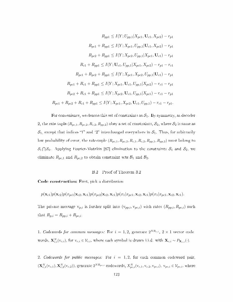
Rpp1 ≤ I(Y ;Upp,1|Xpc1,Uc1, Xpc2)− rp1
Rpc1 +Rpp1 ≤ I(Y ;Xpc1, Upp,1|Uc1, Xpc2)− rp1
Rpc2 +Rpp1 ≤ I(Y ;Xpc2, Upp,1|Xpc1,Uc1)− rp1
Rc1 +Rpp1 ≤ I(Y ;Uc1, Upp,1|Xpc1, Xpc2)− rp1 − rc1
Rpc1 +Rpc2 +Rpp1 ≤ I(Y ;Xpc1, Xpc2, Upp,1|Uc1)− rp1
Rpc1 +Rc1 +Rpp1 ≤ I(Y ;Xpc1,Uc1, Upp,1|Xpc2)− rc1 − rp1
Rpc2 +Rc1 +Rpp1 ≤ I(Y ;Xpc2,Uc1, Upp,1|Xpc1)− rc1 − rp1
Rpc1 +Rpc2 +Rc1 +Rpp1 ≤ I(Y ;Xpc1, Xpc2,Uc1, Upp,1)− rc1 − rp1.
For convenience, we denote this set of constraints as S1. By symmetry, at decoder
2, the rate-tuple (Rpc,1, Rpc,2, Rc,2, Rpp,2) obey a set of constraints, S2, where S2 is same as
S1, except that indices �1� and �2� interchanged everywhere in S1. Thus, for arbitrarily
low probability of error, the rate-tuple (Rpc,1, Rpc,2, Rc,1, Rc,2, Rpp,1, Rpp,2) must belong to
S1∩S2. Applying Fourier-Motzkin [87] elimination to the constraints S1 and S2, we
eliminate Rpc,1 and Rpc,2 to obtain constraint sets B1 and B2.
B.2 Proof of Theorem 3.2
Code construction: First, pick a distribution
p(xc1)p(xc2)p(xpc1|xc2,xc1)p(xpc2|xc2,xc1)p(x1|xpc1,xc2,xc1)p(x1|xpc1,xc2,xc1).
The private message vp,i is further split into (vpp,i, vpc,i) with rates (Rpp,i, Rpc,i) such
that Rp,i = Rpp,i +Rpc,i.
1. Codewords for common messages: For i = 1, 2, generate 2NRc,i , 2 × 1-vector code-
words, XNc,i(vc,i), for vc,i ∈ Vc,i, where each symbol is drawn i.i.d. with Xc,i ∼ PXc,i(·).
2. Codewords for public messages: For i = 1, 2, for each common codeword pair,
(XNc,1(vc,1),X
Nc,2(vc,2)), generate 2
NRpc,i codewords, XNpc,i(vc,1, vc,2, vpc,i), vpc,i ∈ Vpc,i, where
123

each symbol is drawn i.i.d. with Xpc,i ∼ PXpc,i|Xc,1Xc,2(·).
3. Codewords for sub-private messages: At encoder i, i = 1, 2, for each set of common
and public codewords, (XNc,1(vc,1),X
Nc,2(vc,2), X
Npc,i(vc,1, vc,2, vpc,i)), generate 2NRpp,i code-
words, XNi (vc,1, vc,2, vpc,i, vpp,i), for vpp,i ∈ Vpp,i, where each symbol is drawn i.i.d. with
Xi ∼ PXi|Xc,1,Xc,1,Xpc,i(·|xc,1,xc,2, xpc,i).
Codeword assignments are revealed to both the encoders and the decoders.
Encoding and transmission:
Given (vc,1, vc2, vpc,1, vpp,1) = (i, j, k,m), S1 transmits XN1 (i, j, k,m). A similar procedure
is adopted at S2 with index �1� and �2� exchanged.
Decoding: We illustrate the decoding procedure for the decoder of D1. A
similar procedure holds for the other decoder too.
Given the received signal Y N1 , the decoder checks if there exists an unique tuple
(i, j, k, m) and a l, such that
(XN
c,1(i),XNc,2(j), X
Npc,1(i, j, k), X
Npc,2(i, j, l), X
N1 (i, j, k, m), Y N
1
)∈ TN
ϵ (Xc,1Xc,2Xpc,1Xpc,2X1Y1)
and puts out (vc,1, vpc,1, vpp,1) = (i, j, m) as the decoded message set. An error is de-
clared if either such a tuple does not exist or the tuple is not unique.
Analysis: By the symmetry of random code generation, the performance of the codes
does not depend on the message set transmitted. Therefore, without loss of generality, we
assume that message sets v1 = (vpc,1, vc,1, vpp,1) = (1, 1, 1) and v1 = (vpc,2, vc,2, vpp,2) =
(1, 1, 1) are sent. We consider decoding error analysis for only decoder 1. By symmetry,
similar analysis holds for decoder 2. De�ne the event
Ei,j,k,l,m ={(XN
c,1(i),XNc,2(j), X
Npc,1(i, j, k), X
Npc,2(i, j, l), X
N1 (i, j, k,m), Y N
1 )
∈ TNϵ (Xc,1Xc,2Xpc,1Xpc,2X1Y1)
}.
124

i j k l m Constraints
* * * * * Rc1 +Rc2 +Rpc1 +Rpc2 +Rpp1 ≤ I(Y1;X1, Xpc2)
* 1 * * * Rc1 +Rpc1 +Rpc2 +Rpp1 ≤ I(Y1;X1, Xpc2|Xc,2)
1 * * * * Rc2 +Rpc1 +Rpc2 +Rpp1 ≤ I(Y1;X1, Xpc2|Xc,1)
1 1 * * * Rpc1 +Rpc2 +Rpp1 ≤ I(Y1;X1, Xpc2|Xc,1,Xc,2)
1 1 * 1 * Rpc1 +Rpp1 ≤ I(Y1;X1|Xpc2Xc,1,Xc,2)
1 1 1 * * Rpc2 +Rpp1 ≤ I(Y1;X1, Xpc2|Xpc1,Xc,1,Xc,2)
1 1 1 1 * Rpp1 ≤ I(Y1;X1|Xpc2, Xpc1,Xc,1,Xc,1)
Table B.2: Table depicting the error events (i = ∗ if i = 1)
.
Decoding error occurs if either the correct codewords are not typical with the re-
ceived sequence or there is a set of incorrect codewords that are typical with the received
sequence. That is, the �rst error corresponds to Ec11111, and the latter corresponds to∪
{i,j,k,l,m}={1,1,1,1,1}Eijklm. Therefore, we have the probability of error as
Pe,1 = P(Ec11111 ∪
∪{i,j,k,l,m}
={1,1,1,1,1}
Eijklm)
≤ P(Ec1111) +
∑{i,j,k,l,m}
={1,1,1,1,1}
P(Eijklm).
It is clear that, from the AEP [52], P(Ec11111) → 0. Rest of the error events are listed
in Table B.2 along with the rate constraints to achieve Pe,1 < ϵ for any ϵ > 0. Steps to
evaluate these constraints are standard and are omitted here.
Note that constraints corresponding to some events are redundant due to the
fact that the error-free decoding of vpp,1 is possible only if vc,1, vc,2 and vpc,1 are de-
coded correctly. Also, the fact that D1 would not be interested in the error-free decod-
ing of vpc,2, once vpc,1, vc,1 and vpp,1 are decoded without any error, makes the event
(1, 1, 1, l = 1, 1) irrelevant at D1. The above analysis yields the following constraints on
125
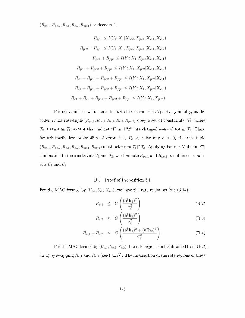
(Rpc,1, Rpc,2, Rc,1, Rc,2, Rpp,1) at decoder 1.
Rpp1 ≤ I(Y1;X1|Xpc2, Xpc1,Xc,1,Xc,2)
Rpc2 +Rpp1 ≤ I(Y1;X1, Xpc2|Xpc1,Xc,1,Xc,2)
Rpc1 +Rpp1 ≤ I(Y1;X1|Xpc2Xc,1,Xc,1)
Rpc1 +Rpc2 +Rpp1 ≤ I(Y1;X1, Xpc2|Xc,1,Xc,2)
Rc2 +Rpc1 +Rpc2 +Rpp1 ≤ I(Y1;X1, Xpc2|Xc,1)
Rc1 +Rpc1 +Rpc2 +Rpp1 ≤ I(Y1;X1, Xpc2|Xc,2)
Rc1 +Rc2 +Rpc1 +Rpc2 +Rpp1 ≤ I(Y1;X1, Xpc2).
For convenience, we denote this set of constraints as T1. By symmetry, at de-
coder 2, the rate-tuple (Rpc,1, Rpc,2, Rc,1, Rc,2, Rpp,2) obey a set of constraints, T2, where
T2 is same as T1, except that indices �1� and �2� interchanged everywhere in T1. Thus,
for arbitrarily low probability of error, i.e., Pe < ϵ for any ϵ > 0, the rate-tuple
(Rpc,1, Rpc,2, Rc,1, Rc,2, Rpp,1, Rpp,2) must belong to T1∩T2. Applying Fourier-Motzkin [87]
elimination to the constraints T1 and T2, we eliminate Rpc,1 and Rpc,2 to obtain constraint
sets C1 and C2.
B.3 Proof of Proposition 3.1
For the MAC formed by (Uc,1, Uc,2, Yd,1), we have the rate region as (see (3.14))
Rc,1 ≤ C
((a†h1)
2
σ2ζ
)(B.2)
Rc,2 ≤ C
((a†h2)
2
σ2ζ
)(B.3)
Rc,1 +Rc,2 ≤ C
((a†h1)
2 + (a†h2)2
σ2ζ
). (B.4)
For the MAC formed by (Uc,1, Uc,2, Yd,2), the rate region can be obtained from (B.2)-
(B.4) by swapping Rc,1 and Rc,2 (see (3.15)). The intersection of the rate regions of these
126

MACs is given by
Rc,1 ≤ min
{C
((a†h2)
2
σ2ζ
), C
((a†h1)
2
σ2ζ
)}(B.5)
Rc,2 ≤ min
{C
((a†h2)
2
σ2ζ
), C
((a†h1)
2
σ2ζ
)}(B.6)
Rc,1 +Rc,2 ≤ C
((a†h1)
2 + (a†h2)2
σ2ζ
). (B.7)
We �rst obtain the optimal power allocation policies for both the sum-rate and
individual rate maximization, and then demonstrate that they are equal.
a. Maximizing the sum-rate:
We know that the sum-rate constraint is
Rc,1 +Rc,2 ≤ C
((h†
1a)2 + (h†
2a)2
σ2ζ
). (B.8)
The goal is to �nd the power allocation vector that maximizes the sum-rate given
by the above equation. This problem can be posed as a constrained problem as
Maximize Rc,1 +Rc,2 subject to ∥a∥2 = Pc.
Since logarithm is increasing in its argument, the above problem is equivalent to
maxa:∥a∥2=Pc
(h†1a)
2 + (h†2a)
2.
Let c = a/√Pc, so that ∥c∥2 = ∥a∥2 /Pc. Also, let
A = h1h†1 + h2h
†2 =
h2 + g2 2hg
2hg h2 + g2
.Then, the optimization problem simpli�es to
maxc:∥c∥2=1
c†Ac,
which is a standard eigenvalue problem. It turns out that the solution (c∗) to the
above problem is the eigenvector corresponding to the maximum eigenvalue (λmax) of
127

the matrix A. We can verify that λmax = (h+ g)2, and
c∗ =[1/√2, 1/√2].
Thus, the optimal power allocation is Pcm = Pcu = Pc/2.
b. Maximizing the individual rates:
Since Pcm = Pc − Pcu, we can observe that, in the RHS of (B.5) or (B.6), the �rst term
is decreasing in Pcm, while the second term is increasing in Pcm. Thus, the maxima for
Rc,1 and Rc,2 are achieved when both the terms of RHS are equal. This is possible only
when Pcm = Pc − Pcm. That is Pcm = Pc/2.
Substituting this into (B.5) and (B.6), and making use of the symmetry in the
rates, we obtain
Rc = min
{C
((h+ g)2 Pc
2σ2ζ
),1
2C
((h+ g)2 Pc
σ2ζ
)}.
Setting z = (h+g)2Pc
σ2ζ
and observing that (1+ z2)
2− (1+z) = z2
4 ≥ 0, we conclude
that
Rc =1
2C
((h+ g)2 Pc
σ2ζ
). (B.9)
B.4 Determining DPC matrices and derivations of (3.11) and (3.12)
The derivation of optimal input covariance matrices applies the techniques in [58]. For
the sake of completeness, we present the derivations in detail here. Considering the
encoding strategy π2, the aim is to design the DPC coe�cients Σ′1,Σ
′2 which maximize
the sum rate given by
Tπ2(Pp, Pp) = maxΣ′1,Σ
′2:
tr(Σ′1+Σ′
2)≤2P ′c
1
2C(h†1Σ
′1h1
)+
1
2C
(h†2Σ
′2h2
1 + h†2Σ
′1h2
),
where for convenience we have normalized the noise variance to unity by letting Σ′1 =
Σ1
σ2ζ,Σ′
2 = Σ2
σ2ζand P ′
c =P−Pp
σ2ζ
. Using the MAC-BC transformation [58], we solve for Σ′1
and Σ′2. To this end, let P1, P2 be the optimal powers allocated for the transmitters in
the corresponding �dual-MAC�. Then, for j = 1, 2, de�ne
Aj = 1 + h†j
j−1∑l=1
Σ′lhj ; Bj = I+
2∑l=j+1
Plhlh†l .
128

Then the optimal covariance matrix is given by
Σ′j = AjPj ·B
− 12
j G†jFjGjF
†jB
− 12
j ,
where Fj , Gj are left and right singular vectors of B− 1
2j hjA
− 12
j obtained by the SVD
B− 1
2j hjA
− 12
j = FjΛjGj .
Consider the dual MAC problem. The dual uplink corresponds to a MAC having
two single antenna users and a receiver with two antennas. We need to �nd optimal
transmit powers P1, P2, that achieve the sum-capacity of the MAC, as the solution to
the following optimization problem.
CMAC = maxP1,P2:
P1+P2≤2P ′c
1
4log(det[I+ P1h1h
†1 + P2h2h
†2
]).
By the symmetric structure in the dual uplink channels, it is clear that allocating
equal power to each user maximizes the sum rate of the system. Thus sum-capacity is
achieved with P1 = P2 = P ′c and with any decoding order. Furthermore, we can verify
that the sum-capacity is
CMAC =1
4log(1 + (h2 − g2)2(P ′
c)2 + 2P ′
c(h2 + g2)
). (B.10)
Now we use the MAC-BC transformations to �nd the covariance matrices (Σ′1,Σ
′2). On
simpli�cation, we obtain
A1 = 1;B1 = I+ P ′ch2h
†2;G1 = 1;F1 =
1
Λ1B
− 12
1 · h1; Λ1 =
√h†1B
−11 · h1
and the covariance matrix Σ′1 is given by
Σ′1 =
P ′c
Λ21
B−11 · h1h
†1B
−11
=P ′c(
1 + P ′c ∥h∥2
) (∥h∥2 + P ′
ch2∆
) h2 (1 + P ′
ch∆)2
gh(1− P ′
c2h2∆
)gh
(1− P ′
c2h2∆
)g2 (1− P ′
ch∆)2
,
where h∆ = h2 − g2.
Similarly, for j = 2,
A2 =∥h∥2
(1 + 2P ′
c ∥h∥2 + P ′
c2h2∆
)(1 + P ′
c ∥h∥2)(∥h∥2 + P ′
ch2∆
) ,B2 = I; G2 = 1; F2 =h2
∥h∥; Λ2 =
√A2 ∥h2∥
129
and the covariance matrix Σ′2 is given by
Σ′2 = P ′
cA2h2h
†2
∥h∥2=
P ′c
(1 + 2P ′
c ∥h∥2 + P ′2c h2
∆
)(1 + P ′
c ∥h∥2) (
∥h∥2 + P ′ch
2∆
) g2 hg
hg h2
.
Now one can easily verify that
P π2c,1 = [Σ1 +Σ2]1,1 = P − Pp; P π2
c,2 = [Σ1 +Σ2]2,2 = P − Pp.
Furthermore, we can verify that
Tπ2(Pp, Pp) =1
4log(1 + (h2 − g2)2(P ′
c)2 + 2P ′
c(h2 + g2)
), (B.11)
which is equal to the sum-capacity of the dual-MAC (B.10).
arks: Note that the covariance matrices Σ1 and Σ2 are of single rank. Thus in
our case, dirty paper coding involving scalar signals is su�cient to achieve the maximum
sum rate. Indeed, by letting b1 =√Pc
Λ1B−1h1, b2 =
√PcA2
h2∥h2∥ , one can obtain vectors
Xc,1 = b1Xc,1 and Xc,2 = b2Xc,2 where Xc,1, Xc,2 are independent Gaussian random
variables of unit variance.
130