optical resonators - columbia...

Optical ResonatorsAPPH E4901/3 Applied Physics Seminar

1

Assignment from Last Week

• What are the resonant optical frequencies of a cube? Numbers please.

• What are the resonant frequencies of an “optical fiber ring”?

• What is a Fabry-Pérot interferometer? And other types of interferometers, … ?

2

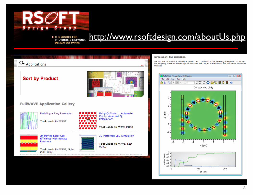
http://www.rsoftdesign.com/aboutUs.php

3

Resonators

• Richard Feynman’s “Cavity Resonators” lecture

• Next week: “The Great Seal Bug Story”

http://www.feynmanlectures.info

http://www.youtube.com/watch?v=j3mhkYbznBk

http://www.youtube.com/watch?v=kd0xTfdt6qw&feature=relmfu

4

23

Cavity Resonators

,

23-1 Real circuit elements

When looked at from anyone pair of terminals, any arbitrary circuit made up of ideal impedances and generators is, at any given frequency, equivalent to a generator 8 in series with an impedance z. That comes about because if we put a voltage V across the terminals and solve all the equations to find the current I, we must get a linear relation between the current and the voltage. Since all the equations are linear, the result for I must also depend only linearly on V. The most genera.llinear form can be expressed as

I I - (V - 8). z (23.1)

In general, both z and 8 may depend in some complicated way on the frequency w. Equation (23.1), however, is the relation we would get if behind the two terminals there was just the generator 8(w) in series with the impedance z(w).

There is also the opposite kind of question: If we have any electromagnetic device at all with two terminals and we measure the relation between I and V to determine 8 and z as functions of frequency, can we find a combination of our ideal elements that is equivalent to the internal impedance z? The answer is that for any reasonable-that is, physically meaningful-function z(w), it is possible to approximate the situation to as high an accuracy as you wish with a circuit containing a finite set of ideal elements. We don't want to ,consider the general problem now, but only look at what might be expected from physical arguments for a feW cases.

If we think of a real resistor, we know that the current through it will produce a magnetic field. So any real resistor should also have some inductance. Also, when a resistor has a potential difference across it, there must be charges on the ends of the resistor to produce the necessary electric fields. As the voltage changes, the charges will change in proportion, so the resistor will also have some capaci-tance. We expect that a real resistor might have the equivalent circuit shown in Fig. 23-1. In a well-designed resistor, the so-called "parasitic" elements Land C are small, so that at the frequencies for which it is intended, wL is much less than R, and l/wCis much greater than R. It may therefore be possible to neglect them. As the frequency is raised, however, they will eventually become important, and a resistor begins to look like a resonant circuit.

A real inductance is also not equal to the idealized inductance, whose impe-dance is iwL. A real coil of wire will have some resistance, so at low frequencies the coil is really equivalent to an inductance in series with some resistance, as shown in Fig. 23-2(a). But, you are thinking, the resistance and inductance are together in a real coil-the resistance is spread all along the wire, so it is mixed in with the inductance. We should probably use a circuit more like the one in Fig. 23-2(b), which has several little R's and L's in series. But the total impedance of such a circuit is just LR + LiwL, which is equivalent to the simpler diagram of part (a).

As we go up in frequency with a real coil, the approximation of an inductance plus a resistance is no longer very good. The charges that must build up on the wires to make the voltages will become important. It is as if there were little con-densers across the turns of the coil, as sketched in Fig. 23-3(a). We might try to approximate the real coil by the circuit in Fig. 23-3(b). At low frequencies, this circuit can be imitated fairly well by the simpler one in part (c) of the figure (which is again the same resonant circuit we found for the high-frequency model of a resistor). For higher frequencies, however, the more complicated circuit of

23-1

23-1 Real circuit elements

23-2 A capacitor at high frequencies

23-3 A resonant cavity

23-4 Cavity modes

23-5 Cavities and resonant circuits

Review: Chapter 23, Vol. I, Resonance Chapter 49, Vol. I, Modes

L

c R

Fig. 23-1. Equivalent circvit of q real resistor.

(0) (b)

Fig .. 23-2. The equivalent circuit of a real inductance at low frequencies.

5

(a)

(b) (c)

Fig. 23-3. The equivalent circuit of a real inductance at higher frequencies.

0

LINES OF E

( 0)

Fig. 23-3 (b) is better. In fact, the more accurately you wish to represent the actual impedance of a real, physical inductance, the more ideal elements you will have to use in the artificial model of it.

Let's look a little more closely at what goes on in a real coil. The impedance of an inductance goes as wL, so it becomes zero at low frequencies-it is a "short circuit": all we see is the resistance of the wire, As we go up in frequency, wL soon becomes much larger than R, and the coil looks pretty much like an ideal induc-tance. As we go'still higher, however, the capacities become important. Their impedance is proportional to l/wC, which is large for small w. For small enough frequencies a condenser is an "open circuit," and when it is in paranel with some-thing else, it ·draws no current. But at high frequencies, the current prefers to flow into the capacitance between the turns, rather than through the inductance. So the current in the coil jumps from one turn to the other and doesn't bother to go around and around where it has to buck the emf. So although we may have intended that the current should go around the loop, it will take the easier path-the path of least impedance.

If the subject had been one of popular interest, this effect would have been called "the high-frequency barrier," or some such name. The same kind of thing happens in all subjects. In aerodynamics, if you try to make things go faster than the speed of sound when they were designed for lower speeds, they don't work. It doesn't mean that there is a great "barrier" there; it just means that the object should be redesigned. So this coil which we designed as an "inductance" is not going to work as a good inductance, but as some other kind of thing at very high frequencies. For high frequencies, we have to find a new design.


Now we want to discuss in detail the behavior of a capacitor-a geometrically ideal capacitor-as the frequency gets larger and larger, so we can see the transition of its properties. (We prefer to use a capacitor instead of an inductance, because the geometry of a pair of plates is much less complicated than the geometry of a coiL) We consider the capacitor shown in Fig. 23-4(a), which consists of two par-allel circular plates connected to an external generator by a pair of wires. If we charge the capacitor with DC, there will be a positive charge on one plate and a negative charge on the other; and there will be a uniform electric field between the plates.

Now suppose that instead of DC, we put an AC of low frequency on the plates. (We will find out later what is "low" and what is "high".) Say we connect the ca-pacitor to a lower-frequency generator. As the voltage alternates, the positive charge on the top plate is taken off and negative charge is put on. While that is happening, the electric field disappears and then builds up in the 9Pposite direction.

SURFACE S

- r- 0 0 , 0 <l9

CURVE f, E t h T 1_ 0 0 0 l' B CURVE f2

liNES OF B

(b)

. . Fig, 23-4. The electric and magnetic fields between the plates of a capacitor. 23-2

6

(a)

(b) (c)

Fig. 23-3. The equivalent circuit of a real inductance at higher frequencies.

0

LINES OF E

( 0)

Fig. 23-3 (b) is better. In fact, the more accurately you wish to represent the actual impedance of a real, physical inductance, the more ideal elements you will have to use in the artificial model of it.

Let's look a little more closely at what goes on in a real coil. The impedance of an inductance goes as wL, so it becomes zero at low frequencies-it is a "short circuit": all we see is the resistance of the wire, As we go up in frequency, wL soon becomes much larger than R, and the coil looks pretty much like an ideal induc-tance. As we go'still higher, however, the capacities become important. Their impedance is proportional to l/wC, which is large for small w. For small enough frequencies a condenser is an "open circuit," and when it is in paranel with some-thing else, it ·draws no current. But at high frequencies, the current prefers to flow into the capacitance between the turns, rather than through the inductance. So the current in the coil jumps from one turn to the other and doesn't bother to go around and around where it has to buck the emf. So although we may have intended that the current should go around the loop, it will take the easier path-the path of least impedance.

If the subject had been one of popular interest, this effect would have been called "the high-frequency barrier," or some such name. The same kind of thing happens in all subjects. In aerodynamics, if you try to make things go faster than the speed of sound when they were designed for lower speeds, they don't work. It doesn't mean that there is a great "barrier" there; it just means that the object should be redesigned. So this coil which we designed as an "inductance" is not going to work as a good inductance, but as some other kind of thing at very high frequencies. For high frequencies, we have to find a new design.


Now we want to discuss in detail the behavior of a capacitor-a geometrically ideal capacitor-as the frequency gets larger and larger, so we can see the transition of its properties. (We prefer to use a capacitor instead of an inductance, because the geometry of a pair of plates is much less complicated than the geometry of a coiL) We consider the capacitor shown in Fig. 23-4(a), which consists of two par-allel circular plates connected to an external generator by a pair of wires. If we charge the capacitor with DC, there will be a positive charge on one plate and a negative charge on the other; and there will be a uniform electric field between the plates.

Now suppose that instead of DC, we put an AC of low frequency on the plates. (We will find out later what is "low" and what is "high".) Say we connect the ca-pacitor to a lower-frequency generator. As the voltage alternates, the positive charge on the top plate is taken off and negative charge is put on. While that is happening, the electric field disappears and then builds up in the 9Pposite direction.

SURFACE S

- r- 0 0 , 0 <l9

CURVE f, E t h T 1_ 0 0 0 l' B CURVE f2

liNES OF B

(b)

. . Fig, 23-4. The electric and magnetic fields between the plates of a capacitor. 23-2

7

I' / r' I I I

/

E

o clw a r

Fig. 23-5. The electric field between the capacitor plates at high frequency, (Edge effects are neglected.)

The integrals are simple if we take them for the curve r 2 , shown in Fig. 23-4(b), which goes up along the axis, out radially the distance r along the top plate, down vertically to the bottom plate, and back to the axis. The line integral of E, around this curve is, of course, zero; so only E2 contributes, and its integral is just -E2(r)' h, where h is the spacing between the plates. (We call E positive if it points upward.) TIlls is equal to the rate of change of the flux of B, which we have to get by an integral over the shaded area S inside r 2 in Fig. 23-4(b). The flux through a vertieal strip of width dr is B(r)h dr, so the total flux is

h f B(r) dr ..

Setting -a/at of the flux equal to the line integral of E 2 , we have

E2 (r) = :t f B(r) dr. (23.6)

Notice that the h cancels out; the fields don't depend on the separation of the plates. Using Eq. (23.5) for B(r), we have

The time derivative just brings down another factor iw; we get

2 2 E ( ) w r E ,.,

2r =-4c2 oe. (23.7)

As we expect, the induced field tends to reduce the electric field farther out. The corrected field E = E, + E2 is then

E = E, + E2 = (1 - w:n Eoe'·'. (23.8)

The electric field in the capacitor is no longer uniform; it has the parabolic shape shown by the broken line in Fig. 23-5. You see that our simple capacitor is getting slightly complicated.

We could now use our results to calculate the impedance of the capacitor at high frequencies. Knowing the electric field, we could compute the charges on the plates and find out how the current through the capacitor depends on the frequency w, but we are not interested in that problem for the moment. We are more interested in seeing what happens as we continue to go up with the frequency -to see what happens at even higher frequencies. Aren't we already finished? No, because we have corrected the electric field, which means that the magnetic field we have calculated is no longer right. The magnetic field of Eq. (23.5) is approximately right, but it is only a first approximation. So let's call it B,. We should then rewrite Eq. (23.5) as

B - iwr E i(>lt 1-2c2 oe. (23.9)

You will remember that this field was produced by the variation of E,. Now the correct magnetic field will be that produced by the total electric field E, + E 2 •

lfwe write the magnetic field as B = B, + B 2 , the second term is just the addi-tional field produced by E 2. To find B2 we can go through the same arguments we have used to find B,; the line integral of B2 around the curve r, is equal to the rate of change of the flux of E2 through r ,. We will just have Eq. (23.4) again with B replaced by B 2 and E replaced by E 2:

c2B 2 ' 21fr = :t (flux of E2 through r,).

Since E2 varies with radius, to obtain its flux we must integrate oyer the circular 23-4

I' / r' I I I

/

E

o clw a r

Fig. 23-5. The electric field between the capacitor plates at high frequency, (Edge effects are neglected.)

The integrals are simple if we take them for the curve r 2 , shown in Fig. 23-4(b), which goes up along the axis, out radially the distance r along the top plate, down vertically to the bottom plate, and back to the axis. The line integral of E, around this curve is, of course, zero; so only E2 contributes, and its integral is just -E2(r)' h, where h is the spacing between the plates. (We call E positive if it points upward.) TIlls is equal to the rate of change of the flux of B, which we have to get by an integral over the shaded area S inside r 2 in Fig. 23-4(b). The flux through a vertieal strip of width dr is B(r)h dr, so the total flux is

h f B(r) dr ..

Setting -a/at of the flux equal to the line integral of E 2 , we have

E2 (r) = :t f B(r) dr. (23.6)

Notice that the h cancels out; the fields don't depend on the separation of the plates. Using Eq. (23.5) for B(r), we have

The time derivative just brings down another factor iw; we get

2 2 E ( ) w r E ,.,

2r =-4c2 oe. (23.7)

As we expect, the induced field tends to reduce the electric field farther out. The corrected field E = E, + E2 is then

E = E, + E2 = (1 - w:n Eoe'·'. (23.8)

The electric field in the capacitor is no longer uniform; it has the parabolic shape shown by the broken line in Fig. 23-5. You see that our simple capacitor is getting slightly complicated.

We could now use our results to calculate the impedance of the capacitor at high frequencies. Knowing the electric field, we could compute the charges on the plates and find out how the current through the capacitor depends on the frequency w, but we are not interested in that problem for the moment. We are more interested in seeing what happens as we continue to go up with the frequency -to see what happens at even higher frequencies. Aren't we already finished? No, because we have corrected the electric field, which means that the magnetic field we have calculated is no longer right. The magnetic field of Eq. (23.5) is approximately right, but it is only a first approximation. So let's call it B,. We should then rewrite Eq. (23.5) as

B - iwr E i(>lt 1-2c2 oe. (23.9)

You will remember that this field was produced by the variation of E,. Now the correct magnetic field will be that produced by the total electric field E, + E 2 •

lfwe write the magnetic field as B = B, + B 2 , the second term is just the addi-tional field produced by E 2. To find B2 we can go through the same arguments we have used to find B,; the line integral of B2 around the curve r, is equal to the rate of change of the flux of E2 through r ,. We will just have Eq. (23.4) again with B replaced by B 2 and E replaced by E 2:

c2B 2 ' 21fr = :t (flux of E2 through r,).

Since E2 varies with radius, to obtain its flux we must integrate oyer the circular 23-4

8

-0.

Fig. 23-6. The Bessel function Jo(xJ.

Then we can write our solution as Eoeiwt times this function, with x = wrlc:

E E iwlT (wr) = oe JQ C . (23.17)

The reason we have called our special function J 0 is that, naturally, this is not

the first time anyone has ever worked out a problem with oscillations in a cylinder.

The function has come up before and is usually called J o. It always comes up

whenever you solve a problem about waves with cylindrical symmetry. The func-

tion J 0 is to cylindrical waves what the cosine function is to waves on a straight

line. So it is an important function, invented a long time ago. Then a man named

Bessel got his name attached to it. The subscript zero means that Bessel invented

a whole lot of different functions and this is just the first of them.

The other functions of Bessel-J"J2 , and so on-have to do with cylindrical

waves which have a variation of their strength with the angle around the axis of

the cylinder. The completely corrected electric field between the plates of our circular

capacitor, given by Eq. (23.17), is plotted as the solid line in Fig. 23":5. For

frequencies that are not too high, our second approximation was already quite

good. The third approximation was even better--so good, in fact, that if we had

plotted it, you would not have been able to see the difference between it and the

solid curve, You will see in the next section, however, that the complete series is

needed to get an accurate description for large radii, or for high frequencies.

23-3 A resonant cavity

We want to look now at what our solution gives for the electric field between

the plates of the capacitor as we continue to go to higher and higher frequencies.

For large w, the parameter x wr/c also gets large, and the first few terms in the

series for Jo of x will increase rapidly. That means that the parabola we have

drawn in Fig. 23-5 curves downward more steeply at higher frequencies. In fact,

it looks as though the field would fall all the way to zero at some high frequency,

perhaps when c/w is approximately one-half of a. Let's see whether Jo does indeed

go through zero and become negative. We begin by trying x 2:

Jo(2) I - I + It - 0'6 0.22.

The function is still not zero, so let's try a higher value of x, say, x 2.5. Putting

in numbers, we write

J 0(2.5) I - 1.56 + 0.61 - 0.09 -0.04.

The function J o has already gone through zero by the time we get to x 2.5.

Comparing the results for x 2 and x 2.5, it looks as though J 0 goes through

zero at one-fifth of the way from 2.5 to 2. We would guess that the zero occurs for

x approximately equal to 2.4. Let's see what that value of x gives:

J 0(2.4) I - 1.44 + 0.52 - 0.08 0.00.

We get zero to the accuracy of our two decimal places. If we make the calculation

more accurate (or since Jo is a well-known function, if we look it up in a book), we

find that it goes through zero at x 2.405. We have worked it out by hand to

show you that you too could have discovered these things rather than having to

borrow them from a book. As long as we are looking up Join a book, it is interesting to notice how it

goes for larger values of x; it looks like the graph in Fig. 23-6. As x increases,

Jo(x) oscillates between positive and negative values with a decreasing amplitude

of oscillation. We have gotten the following interesting resuIt: If we go high enough in fre-

quency, the electric tidd at the center of our condenser will be one way and the

electric field near the edge will point in the opposite direction. For example,

23-6

9

suppose that we take an w high enough so that x wr 1 c at the outer edge of the capacitor is equal to 4; then the edge of the capacitor corresponds to the abscissa x 4 in Fig. 23-6. This means that our capacitor is being operated at the fre-quency w 4cl a. At the edge of the plates, the electric field will have a rather high magnitude opposite the direction we would expect. That is the terrible thing that can happen to a capacitor at high frequencies. Ifwe go to very high frequencies, the direction of the electric field oscillates back and forth many times as we go out from the center of the capacitor. Also there are the magnetic fields associated with these electric fields. It is not surprising that our capacitor doesn't look like the ideal capacitance for high frequencies. We may even start to wonder whether it looks more like a capacitor or an inductance. We should emphasize that there are even more complicated effects that we have neglected which happen at the edges of the capacitor. For instance, there will be a radiation of waves out past the edges, so the fields are even more complicated than the ones we have computed, but we will not worry about those effects now.

We could try to figure out an equivalent circuit for the capacitor, but perhaps it is better if we just admit that the capacitor we have designed for low-frequency fields is just no longer satisfactory when the frequency is too high. If we want to treat the operation of such an object at high frequencies, we should abandon the approximations to Maxwell's equations that we have made for treating circuits and return to the complete set of equations which describe completely the fields in space. Instead of dealing with idealized circuit elements, we have to deal with the real conductors as they are, taking into account all the fields in the spaces in between. For instance, if we want a resonant circuit at high frequencies we will not try to design one using a coil and a parallel-plate capacitor.

We have already mentioned that the paralIel-plate capacitor we have been analyzing has some of the aspects of both a capacitor and an indnctance. With the electric field there are charges on the surfaces of the plates, and with the magnetic fields there are back emf's. Is it possible that we already have a resonant circuit? We do indeed. Suppose we pick a frequency for which the electric field pattern

to zero at some radius inside the edge of the disc; that is, we choose wal c greater than 2.405. Everywhere on a circle c'oaxial with the plates the electric field will be zero. Now snppose we take a tbin metal sheet and cut a strip just wide enough to fit between the plates of the capacitor. Then we bend it into a cylinder that will go around at the radius where the electric field is zero. Since there are no electric fields there, when we put this conducting cylinder in place, no currents will flow in it; and there will be no changes in the electric and magnetic fields. We have been able to put a direct short circUlt across the capacitor without changing

And look wbat we have; we have a complete cylindrical can with elec-tridal and magnetic fields inside and no connection at all to the outside world. The fields inside won't change even if we throwaway the edges of the plates outside our can, and also the capacitor leads. All we have left is a closed can with electric and magnetic fields inside, as shown in Fig. 23-7(a). The electric fields are os-cillating back and forth at the frequency w-which, don't forget, determined the diameter of the can. The amplitude of the oscillating Efield varies with the distance from the axis of the can, as shown in the graph of Fig. 23-7(b). This curve is just the first arch of the Bessel function of zero order. There is also a magnetic field which goes in circles around the axis and oscillates in time 90° out of phase with the electric field.

We can also write out a series for the magnetic field and plot it, as shown in the graph of Fig. 23-7(c).

How is it that we can have an electric and magnetic field inside a can with no external connections? It is because the electric and magnetic fields maintain them-selves: the changing E makes a B and the changing B makes an E-all according to the equations of Maxwell. The magnetic field has an inductive aspect, and the electric field a capacitive aspect; together they make something like a resonant circnit. Notice that the conditions we have described would only happen if the radius of the can is exactly 2.405 c/w. For a can of a given radius, the oscillating electric and magnetic fields will maintain themselves-in the way we have described

23-7

0

t i 0

(b)

(c)

0

0 +

1.0

cBe 1.0

- -0

0 + +

LINES OF ii /' - -® ®

it ® ® ®

+ + + LINES OF

( 0)

2.405-clw r

r

Fig. 23-7. The electric and magnetic fields in an enclosed cylindrical can.

10

INPUT LOOP

OUTPUT LOOP

Fig. 23-8. Coupling into and out of a resonant cavity.

R·F SIGNAL

GENERATOR

Fig. 23-9. A setup for observing the cavity resonance.

>-z ... cr cr :0 U

>-:0 .. >-5 llw = wo/Q

Wo Frequency

Fig. 23-10. The frequency response curve of a resonant cavity.

at that particular frequency. So a cylindrical can of radius r is resonant at the frequency c

Wo = 2.405 -. r (23.18)

We have said that the fields continue to oscillate in the same way after the can is completely closed. That is not exactly right. It would be possible if the walls of the can were pe(fect conductors. For a real can, however, the oscillating cur-rents which exist on the inside walls of the can lose energy because of the resistance of the material. The oscillations of the fields will gradually die away. We can see from Fig. 23-7 that there must be strong currents associated with electric and magnetic fields inside the cavity. Because the vertical electrical field stops suddenly at the top and bottom plates of the can, it has a large divergence there; so there must be positive and negative electric charges on the inner surfaces of the can, as shown in Fig. 23-7(a). When the electric field reverses, the charges must reverse also, so there must be an alternating current between the top and bottom plates of the can. These charges will flow in the sides of the can, as shown in the figure. We can also see that there must be currents in the sides of the can by considering what happens to the magnetic field. The graph of Fig. 23-7(c) tells us that the magnetic field suddenly drops to zero at the edge of the can. Such a sudden change in the magnetic field can happen only if there is a current in the wall. This current is what gives the alternating electric charges on the top and bottom plates of the can.

You may be wondering about our discovery of currents in the vertical sides of the can. What about our earlier statement that nothing would be changed when we introduced these vertical sides in a region where the electric field was zero? Re-member, however, that when we first put in the sides of the can, the top and bottom plates extended out beyond them, so that there were also magnetic fields on the outside of our can. It was only when we threw away the parts of the capacitor plates beyond the edges of the can that net currents had to appear on the insides of the vertical walls.

Although the electric and magnetic fields in the completely enclosed can will gradually die away because of the energy losses, we can stop this from happening if we make a little hole in the can and put in a little bit of electrical energy to make up the losses. We take a small wire, poke it through the hole in the side ofthe can, and fasten it to the inside wall so that it makes a small loop, as shown in Fig. 23-8. If we now connect this wire to a source of high-frequency alternating current, this current will couple energy into the electric and magnetic fields of the cavity and keep the oscillations going. This will happen, of course, only if the frequency of the driving source is at the resonant frequency of the can. If the source is at the wrong frequency, the electric and magnetic fields will not resonate, and the fields in the can will be very weak.

The resonant behavior can easily be seen by making another small hole in the can and hooking in another coupling loop, as we have also drawn in Fig. 23-8. The changing magnetic field through this loop will generate an induced electro-motive force in the loop. If this loop is now connected to some external measuring circuit, the currents will be proportional to the strength of the fields in the cavity. Suppose we now connect the input loop of our cavity to an RF signal generator, as shown in Fig. 23-9. The signal generator contains a source of alternating current whose frequency can be varied by varying the knob on the front of the generator. Then we connect the output loop of the cavity to a "detector," which is an instru-ment that measures the current from the output loop. It gives a meter reading pro-portional to this current. If we now measure the output current as a function of the frequency of the signal generator, we find a curve like that shown in Fig. 23-10. The output current is small for all frequencies except those very near the frequency Wo, which is the resonant frequency of the cavity. The resonance curve is very much like those we described in Chapter 23 of Vol. I. The width of the resonance is, however, much narrower than we usually find for resonant circuits made of induc-tances and capacitors; that is, the Q of the cavity is very high. It is not unusual to find Q's as high as 100,000 or more if the inside walls of the cavity are made of some material with a very good conductivity, such as silver. 23-8

11

23-4 Cavity modes

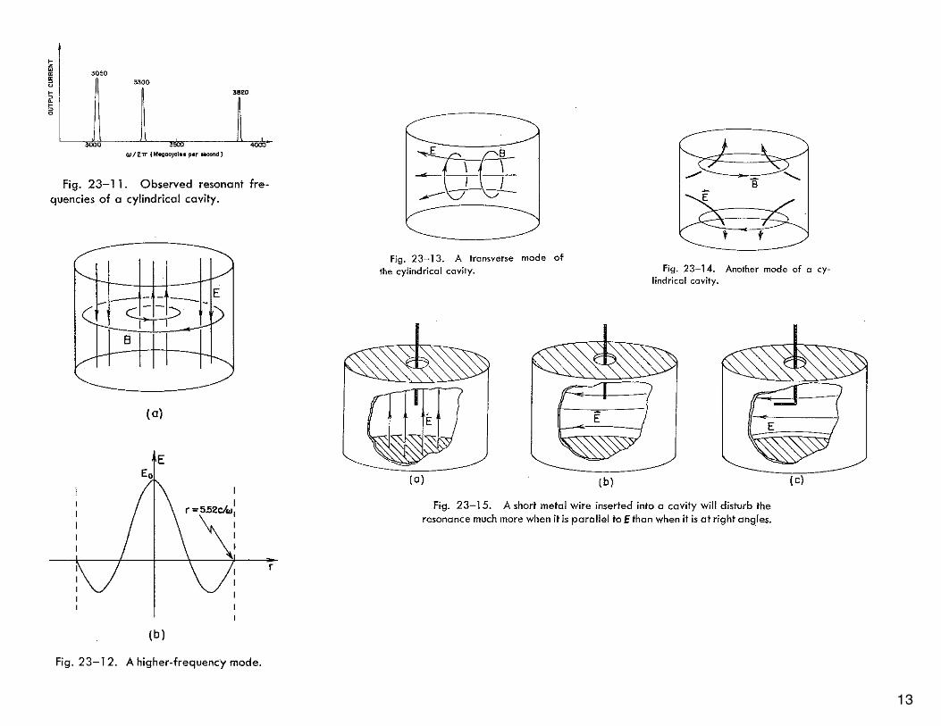
Suppose we now try to check our theory by making measurements with an actnal can. We take a can which is a cylinder with a diameter of 3.0 inches and a height of about 2.5 inches. The can is fitted with an input and output loop, as shown in Fig. 23-8. If we calculate the resonant frequency expected for this can according to Eq. (23.18), we get that fa = wo/27r = 3010 megacycles. When we set the frequency of our signal generator near 3000.jllegacycles and vary it slightly until we find the resonance, we observe that the maximnm output current occurs for a frequency of 3050 megacycles, which is quite close to the predicted resonant frequency, but not exactly the same. There are several possible reasons for the discrepancy. Perhaps the resonant frequency is changed a little bit because of the lioles we have cut to put in the coupling loops. A little thought, liowever, shows that the holes sliould lower the resonant frequency a little bit, so that cannot be the reason. Perhaps there is some slight error in the frequency calibration of the signal generator, or perhaps our measurement of the diameter of the cavity is not accurate enough. Anyway, the agreement is fairly close.

Mucli more important is something that happens if we vary the frequency of our signal generator somewhat further from 3000 megacycles. When we do that we get the results shown in Fig. 23-11. We find that, in addition to the resonance we expected near 3000 megacycles, there is also a resonance near 3300 megacycles and one near 3820 megacycles. What do these extra resonances mean? We might get a clue from Fig. 23-6. Although we have been assuming that the first zero of the Bessel function occurs at the edge of the can, it could also be that the second zero of the Bessel function corresponds to the edge of tlie can, so that there is one complete oscillation of the electric field as we move from tlie center of the can out to the edge, as shown in Fig. 23-12. This is another possible mode for the oscillating fields. We should certainly expect the can to resonate in such a mode. But notice, the second zero of tlie Bessel function occurs at x = 5.52, whicli is over twice as large as the value at the first zero. The resonant frequency of this mode should therefore be higher tlian 6000 megacycles. We would, no doubt, find it there, but it doesn't explain the resonance vie observe at 3300.

The trouble is that in our analysis ofthe behavior of a resonant cavity we have considered only one possible geometric arrangement of the electric and magnetic fields. We have assumed that the electric fields are vertical and that the magnetic fields lie in horizontal circles. But other fields are possible. The ouly requirements are that the fields should satisfy MaxweII's equations inside the can and that the electric field should meet the wa11 at right angles. We have considered the case in which the top and the bottom of the can are flat, but things would not be completely different if the top and bottom were curved. In fact, how is the can supposed to know which is its top and bottom, and which are its sides? It is, in fact, possible to show that there is a mode of osci11ation of the fields inside the can in which the electric fields go more or less across the diameter ofthe can, as shown in Fig. 23-13.

It is not too hard to understand why the natural frequency of this mode should be not very different from the natural frequency of the first mode we have considered. Suppose that instead of our cylindrical cavity we had taken a cavity which was a cnbe 3 inches on a side. It is clear that this cavity would have three different modes, but a11 with the same frequency. A mode with the electric field going more or less up and down would certainly have the same frequency as the mode in which the electric field was directed right and left. If we now distort the cube into a cylinder, we will change these frequencies somewhat. We would stilI expect them not to be changed too mnch, provided we keep the dimensions of the cavity more or less the same. So the frequency of the mode of Fig. 23-13 should not be too different from the mode of Fig. 23-8. We could make a detailed cal-culation of the naturalfrequency of the mode shown in Fig. 23-13, but we will not do that now. When the calculations are carried through, it is found that, for the dimensions we have assumed, the resonant frequency comes out very close to the observed resonance at 3300 megacycles.

By similar calculations it is possible to show that there should be still another mode at the other resonant frequency we (ound near 3800 megacycles. For this

23-9

3050 3300

""

'"'' ,= QJ I Z 1T (M"IIac)",l .. per HCOnd}

Fig. 23-11. Observed resonant fre-quencies of a cylindrical cavity.

----- E

( 0)

E

r

(b)

Fig, 23-12. A higher-frequency mode.

---- I J

Fig. 23-13. A transverse mode of the cylindrical cavity.

12

23-4 Cavity modes






23-9

3050 3300

""



----- E

( 0)

E

r

(b)


---- I J


23-4 Cavity modes






23-9

3050 3300

""



----- E

( 0)

E

r

(b)


---- I J


mode, the electric and magnetic fields are as shown in Fig. 23-14. The electric field does not bother to go all the way across the cavity. It goes from the sides to the ends, as shown.

/------B

As you will probably now believe, if we go higher and higher in frequency we should expect to find more and more resonances. There are many different modes, each of which will have a different resonant frequency corresponding to some par-ticular complicated arrangement of the electric and magnetic fields. Each of these field arrangements i. called a resonant mode. The resonance frequency of each mode can be calculated by solving Maxwell's equations for the electric and magnetic fields in the cavity.

E

Fig. 23-14. lindrical cavity.

t f

Another mode of a cy-

When we have a resonance at some particular frequency, how can we know which mode is being excited? One way is to poke a little wire into the cavity through a small hole. If the electric field is along the wire, as in Fig. 23-15(a), there will be relatively large currents in the wire, sapping energy from the fields, and the resonance will be suppressed. If the electric field is as shown in Fig. 23-15(b), the wire will have a much smaller effect. We could find which way the field points in this mode by bending the end of the wire, as shown in Fig. 23-15( c). Then, as we rotate the wire, there will be a big effect when the end of the wire is parallel to E and a small effect when it is rotated so as to be at 90' to E.

(b)

Fig. 23-15. A short metal wire inserted into a cavity will disturb the resonance much more when it is parallel to E than when it is at right ang.'es.


( c)

Although the resonant cavity we have been describing seems to be quite different from the ordinary resonant circuit consisting of an inductance and a capacitor, the two resonant systems are, of course, closely related. They are both members of the same family; they are just two extreme cases of electromagnetic resonators-and there are many intermediate cases between these two extremes. Suppose we start by considering the resonant circuit of a capacitor in parallel with an inductance, as shown in Fig. 23-16(a). This circuit will resonate althe frequency Wo = I/VLC. If we want to raise the resonant frequency of this circuit, we can do so by lowering the inductance L. One way is to decrease the number of turns in the coil. We can, however, go only so rar in this direction. Eventually we will get down to the last turn, and we will have just a piece of wire joining the top and bottom plates of the condenser. We could raise the resonant frequency still further by making the capacitance smaller; however, we can also continue to decrease the inductance by putting several inductances in parallel. Two one-turn inductances in parallel will have only half the inductance of each turn. So when our inductance has been reduced to a single turn, we can continue to raise the resonant frequency by adding other single loops from the top plate to the bottom plate of the condenser. F6r instance, Fig. 23-16(b) shows the condenser plates connected by six such "'single-turn inductances." If we continue to add many such pieces of wire, we can make the transition to the completely enclosed resonant system shown in part (c) of the figure, which is a drawing of the cross section of a cylindrically symmetrical 23-10

mode, the electric and magnetic fields are as shown in Fig. 23-14. The electric field does not bother to go all the way across the cavity. It goes from the sides to the ends, as shown.

/------B

As you will probably now believe, if we go higher and higher in frequency we should expect to find more and more resonances. There are many different modes, each of which will have a different resonant frequency corresponding to some par-ticular complicated arrangement of the electric and magnetic fields. Each of these field arrangements i. called a resonant mode. The resonance frequency of each mode can be calculated by solving Maxwell's equations for the electric and magnetic fields in the cavity.

E

Fig. 23-14. lindrical cavity.

t f

Another mode of a cy-

When we have a resonance at some particular frequency, how can we know which mode is being excited? One way is to poke a little wire into the cavity through a small hole. If the electric field is along the wire, as in Fig. 23-15(a), there will be relatively large currents in the wire, sapping energy from the fields, and the resonance will be suppressed. If the electric field is as shown in Fig. 23-15(b), the wire will have a much smaller effect. We could find which way the field points in this mode by bending the end of the wire, as shown in Fig. 23-15( c). Then, as we rotate the wire, there will be a big effect when the end of the wire is parallel to E and a small effect when it is rotated so as to be at 90' to E.

(b)

Fig. 23-15. A short metal wire inserted into a cavity will disturb the resonance much more when it is parallel to E than when it is at right ang.'es.


( c)

Although the resonant cavity we have been describing seems to be quite different from the ordinary resonant circuit consisting of an inductance and a capacitor, the two resonant systems are, of course, closely related. They are both members of the same family; they are just two extreme cases of electromagnetic resonators-and there are many intermediate cases between these two extremes. Suppose we start by considering the resonant circuit of a capacitor in parallel with an inductance, as shown in Fig. 23-16(a). This circuit will resonate althe frequency Wo = I/VLC. If we want to raise the resonant frequency of this circuit, we can do so by lowering the inductance L. One way is to decrease the number of turns in the coil. We can, however, go only so rar in this direction. Eventually we will get down to the last turn, and we will have just a piece of wire joining the top and bottom plates of the condenser. We could raise the resonant frequency still further by making the capacitance smaller; however, we can also continue to decrease the inductance by putting several inductances in parallel. Two one-turn inductances in parallel will have only half the inductance of each turn. So when our inductance has been reduced to a single turn, we can continue to raise the resonant frequency by adding other single loops from the top plate to the bottom plate of the condenser. F6r instance, Fig. 23-16(b) shows the condenser plates connected by six such "'single-turn inductances." If we continue to add many such pieces of wire, we can make the transition to the completely enclosed resonant system shown in part (c) of the figure, which is a drawing of the cross section of a cylindrically symmetrical 23-10

13

liNES OF 8 ...-'

8

i I

0 "e" r

L

0 0 :'\ -

0 0 LINES OF E

I -

h

1 (0) (c)

fig. 23-16. Resonators of progressively higher resonant frequencies.

object. Our inductance is now a cylindrical hollow can attached to the edges of the condenser plates. The electric and magnetic fields will be as shown in the figure. Such an object is, of conrse, a resonant cavity. It is called a "loaded" cavity. But we can still think of it as an L-C circuit in which the capacity section is the region where we find most of the electric field and the inductance section is that region where we find most of the magnetic field.

If we want to make the frequency of the resonator in Fig. 23-16(c) still higher, we can do so by continuing to decrease the inductance L. To do that, we must decrease the geometric dimensions of the inductance section, for example by decreasing the dimension h in the drawing. As h is decreased, the resonant fre-quency will be increased. Eventually, of course, we will get to the situation in which the height h is just equal to the separation between the condenser plates. We then have just a cylindrical can; our resonant circuit has become the cavity resonator of Fig. 23-7.

You will notice that in the original L-c resonant circuit of Fig. 23-16 the electric and magnetic fields are quite separate. As we have gradually modified the resonant system to make higher and higher frequencies, the magnetic field has been brought closer and closer to the electric field until in the cavity resonator the two are quite intermixed.

II II L

® ®

® ®

® ®

Although the cavity resonators we have talked about in this chapter have been cylindrical cans, there is nothing magic about the cylindrical shape. A can of any shape will have resonant frequencies corresponding to various possible modes of oscillations of the electric and magnetic fields. For example, the "cavity" shown in Fig. 23-]7 will have its own particular set of resonant frequencies-although they would be rather difficult to calculate. Fig. 23-17. Another resonant cavity.

23-11

14

Next Week

On May 26, 1960, U.S. Ambassador to the United Nations Henry Cabot Lodge, Jr. unveiled the Great Seal Bug before the UN Security Council to counter Soviet denunciations of American U-2 espionage. The Soviets had presented a replica of the Great Seal of the United States as a gift to Ambassador Averell Harriman in 1946. The gift hung in the U.S. Embassy for many years, until in 1952, during George F. Kennan's ambassadorship, U.S. security personnel discovered the listening device embedded inside the Great Seal. Lodge's unveiling of this Great Seal before the Security Council in 1960 provided proof that the Soviets also spied on the Americans, and undercut a Soviet resolution before the Security Council denouncing the United States for its U-2 espionage missions

15

optical resonators - columbia...

Documents