1

Optimal constant acceleration motion primitivesGregor Klancar and Sašo Blažic

Abstract—This article proposes new motion primitives that aretime-optimal and feasible for a vehicle (wheeled-mobile robot).They are parameterized by a constant acceleration and a constantdeceleration in an obstacle-free environment between an initialand a final configuration with given poses and velocities. Thederived compact parametric solution has implicit optimal velocityprofile, is continuous in C2, considers driving constraints and iscomputationally efficient. The path is derived analytically con-sidering constraints on maximal allowable driving velocity andaccelerations. The obtained motion primitives have continuoustransition of curvature and are thus easily drivable by the vehicle.

The proposed motion primitives are evaluated on several path-planning examples and obtained solutions are compared to anumerically expensive planner using Bernstein-Bézier (BB) curvewith path shape and velocity profile optimization. Numerousexperiments have been conducted not only in the simulationenvironment but also during testing and comparisons on theactual mobile robot platforms. It is shown that the proposedsolution is computationally efficient, time optimal under givenconstraints and trapezoidal velocity profile assumptions and isclose to globally optimal solution with an arbitrary velocityprofile.

Index Terms—Path planning, motion primitives, minimal time,driving constraints.

I. INTRODUCTION

Path planning is a fundamental task of any autonomousmobile vehicle and has been extensively studied in the litera-ture. The majority of existing path planners provide solutionsdescribed by a set of way-points [1], [2]. Such a path isoften not feasible and may result in control tracking errorsand uncomfortable driving due to sudden acceleration changesinvolved [3]. Although such simple solutions might be suffi-cient for several applications, this is not desired in perfor-mance demanding applications where comfortable driving (e.g.wheelchairs or self-driving cars), minimal-time driving or lowactuator wear for robust long-time performance is preferred[4], [5]. To obtain semi feasible paths (e.g. with smooth veloc-ities or curvature) in obstructed environments usually a fixedset of motion primitives is used to build a state lattice graphwhere path is searched [2], [6], [7]. Obtained paths minimizedefined criteria, e.g., minimal distance, maximal clearance,energy or similar in the applied space discretization. However,finding globally minimal-time solutions or at lest sufficientapproximations with a numeric search is computationally tooexpensive.

Shortest path planning in obstacle free environment hasachieved wide attention. The first works on shortest paths forcurvature-constrained vehicles are done by [8], [9] and [1].An optimal control law that steers the robot on a shortest

G. Klancar and S. Blažic are with Faculty of Electrical Engineering,University of Ljubljana, Tržaška 25, SI-1000 Ljubljana, Slovenia e-mail:gregor.klancar@fe.uni-lj.si

distance to the goal is provided in [10]. Shortest paths studyfor wheeled robots with field-of-view constraints has beenreported in [11]. Recently, also minimal energy path planinghas drawn considerable attention to maximize mobile robotperformance considering its limited on-board power [12], [13].

However, similar application of feasible minimal-time pathplanning to wheeled mobile robots are rare. More commonare non-smooth (with discontinuity in curvature or orientation)planning approaches resulting in minimal distance or minimaltime paths; or smooth planners which are not optimal in thesense of distance or time. Besides circular arcs and straightmotion also several smooth motion primitives applicable inpath planning or path smoothing were suggested, such asBezier curves [2], [14], clothoids [15], higher order polyno-mials [16] and eta-spline motion primitives with continuousaccelerations [4], [17]. Some approaches apply path-velocitydecomposition to compute admissible velocity profile thatminimize time on a predefined path [18]–[21].

Time-optimal trajectory planning considering bounded ve-locities of the differential drive’s wheels which can be dis-continuous is proposed in [22]. Minimal-time trajectory for arobot with bounded acceleration where at least five switchedsequences are applied in bang- bang control is proposed in[23]. A geometric reasoning is applied by [24] to obtaintime-optimal trajectories for bidirectional steered robot. Suchminimal-time path planners usually assume unobstructed en-vironments and find a trajectory between the given initial andthe final configuration. As shown in [25] maximal-accelerationbang-bang trajectories obtained numerically following Pon-tryagin’s maximum principle are time-optimal candidates. Butdue to increased complexity of multiple DOF, minimal-timesolutions quickly become too complex to be solved analyti-cally.

This article addresses optimal time trajectory planning fora wheeled vehicle in a free space with given initial and finalposes and velocities and considering constraints on velocityand acceleration. In the similar existing works [22]–[25] thenecessary conditions for existence of the globally time-optimaltrajectories are given which combine several controls that areeither wheel’s maximal velocities [22], or wheel’s maximalaccelerations [23], [25], or turning radii [24]. The obtainedtrajectories do not have continuous curvature and describesthe trajectory as a sequence of discontinuous controls. Ourapproach assumes single switch from constant-accelerated toconstant-decelerated (CACD) motion restricted by a slip-free-driving requirement and derives the time-optimal solutionconsidering those assumptions. The obtained optimal trajec-tory is a parametric function of the two accelerations andit has continuous curvature. The main idea is illustrated bythe proposed basic solution that considers trapezoidal velocityprofile with a constant-acceleration section, a constant-velocity

2

section and a constant-deceleration section. Extensions of thisbasic approach are proposed to obtain solutions where not onlythe velocity and acceleration are bounded but also continuouscurvature of the trajectories is guaranteed.

The obtained minimal time trajectory is a parametric func-tion of time where optimal velocity profile is implicitly definedby the solution. The solution is therefore obtained in onestep. No additional velocity optimization is required in thesecond step as in [18] or [19]. To find the optimal solutiononly two equations need to be solved for two unknownparameters (constant acceleration and constant deceleration).The solution is found numerically in a bounded space of thesetwo parameters. This lowers the complexity compared to astrictly numeric solution where optimal solution is found byoptimization of three or more variables (e.g. maximal velocity)and applying numeric simulations of the vehicle kinematicmodel to compute robot trajectories in each iteration of theoptimization. Thus the obtained solution is computationallyefficient and compact. It assumes trapezoidal velocity profilewith constant accelerations and bounded maximal velocity andacceleration constraints. It is shown that these assumptionsapplied in the proposed CACD path planner produces resultswhich are very close to the globally optimal solutions, i.e. thesolutions where the path is completely arbitrary. To evaluateand compare results the fifth order Bernstein-Bézier (BB)curve planner is applied with four free parameters definedby optimization of path and velocity profile to minimize thetravelling time.

The proposed CACD motion primitives can have severalapplications. It can be used to smooth robot paths which aredefined by a set of straight line segments with discontinuousorientation. Such a path is usually the output of many pathplanners in environment with known obstacles. Similarly isdone in [26], [15] where apply clothoids to obtain necessaryconditions for the locally time-optimal smoothing primitives.It can be used to plan trajectories in unobstructed environmentsfrom initial to desired final configuration in a smooth and time-optimal fashion. It can also be applied to smooth path plannersin obstructed environments to compute cost-to-goal heuristicssuch as in [5] or to use CACD primitives with continuoustransitions of curvature to build a lattice graph for optimal pathsearching algorithms as in [5]–[7] or in kinodynamic RRT∗

planners [3], [27], [28].

II. DRIVING CONSTRAINTS

When searching for the minimal time the main goal oftrajectory planing is to compute a path with a velocity profilethat is easily drivable by mobile robots and achieves the targetpose within a reasonable time. When optimizing driving timea vehicle needs to maximize its velocity v. The maximalvelocity vMAX that the vehicle can achieve is always limitedin practice. The acceleration (the rate of change of velocity)is also limited not only because of robot capabilities but alsoto prevent lateral and longitudinal slip. Maximal tangentialacceleration imposed by the drive is usually higher than theone required by the slip-free driving. We will therefore con-centrate on the acceleration constraints imposed by slippingin the sequel.

Tangential acceleration at = dvdt in a straight motion is

constrained by maximal tangential acceleration aMAXt wherethe torque on the wheels produces the force in the groundcontact that is lower or equal to the friction force. Whendriving on a curved path (with the curvature κ) with a constanttangential velocity v and an angular velocity ω, the radialacceleration ar = vω = v2κ is constrained by maximal radialacceleration aMAXr to have the centrifugal force lower than thewheel lateral friction force. Combining tangential and radialaccelerations, slipping is avoided if the radial acceleration andthe tangential acceleration are kept inside the ellipse definedby aMAXt and aMAXr:

a2t

a2MAXt

+a2r

a2MAXr

≤ 1 (1)

Optimality in the sense of driving time therefore requiresdriving on the boundary of ellipse defined by (1) [18], [19].When vMAX is achieved, acceleration might not be on theboundary of the ellipse (1) but rather inside of the ellipse.

III. OPTIMAL CONSTANT ACCELERATION CURVES

The idea is to follow similar strategy as the one resultedfrom by Pontryagin’s principle applied on a double integrator.The vehicle applies maximum acceleration for some time andmaximum deceleration for some time to reach the desired lo-cation. It has been shown in [25] that the trajectories obtainedon differential drive using maximal accelerations are time-optimal candidates. Optimality was evaluated using a numericprocedure where robot path was simulated using numericintegration of robot kinematics and numeric examination ofidentified sets of time-optimal trajectories.

In the proposed approach we derive parametric equations forthe optimal-time trajectory analytically and then solve themto compute the required maximal accelerations as follows.Maximal constant acceleration is defined by a point (at1, ar1)on the ellipse (1) with at1 > 0 and maximal decelerationby another point (at2, ar2) with at2 < 0. Without loss ofgenerality1 let us assume the vehicle is initially located inthe origin with its orientation pointing in the direction ofx axis (xsp = ysp = 0, θsp = 0), and has velocity vsp,while the desired end pose and velocity are xep, yep, θep,and vep, respectively. The main goal is to find such constantacceleration pair (at1, ar1) and constant deceleration pair(at2, ar2) to reach the desired end pose within a minimal timewhich implies that both pairs need to fulfill relation (1).

A. Curve definition

The trajectory obtained during acceleration is defined bytangential velocity v1(t) = vsp+at1t, angular velocity ω1(t) =ar1v1(t) = ar1

vsp+at1tand vehicle’s differential drive kinematics

x(t) = v(t) cos(θ(t))y(t) = v(t) sin(θ(t))

θ(t) = ω(t)(2)

1Such initial condition is easily achieved by a simple affine coordinatetransformation.

3

Note that the approach presented in this paper does not onlyapply to differentially driven mobile robots but also to amuch more general class of wheeled mobile robots whoseinput commands can be expressed as u1 = f(v, ω) andu2 = g(v, ω) where f(·) and g(·) are smooth functionsof v and ω. For example, in the case of a car-like robotwith the front wheel steering angle and velocity commands:u2 = α = arctan ωd

v and u1 = vs = vcosα where d is the

distance between the front and the rear wheels axes whilethe steering angle is limited due to practical implementation(|α| < αMAX ). Consequently, the maximal curvature of thepath is also limited (κMAX = tanαMAX

d ) and the obtainedacceleration solutions need to fulfill the curvature constraint inthe start pose ar1

v2sp≤ κMAX and in the end pose ar2

v2ep≤ κMAX .

Considering (2) trajectory during acceleration reads

θ1(t) =

∫ t

0

ω1(τ)dτ =ar1at1

lnv1(t)

vsp(3)

x1(t) =

∫ t

0

v1(τ) cos θ1(τ)dτ

=v2

1(t) (2at1 cos θ1(t) + ar1 sin θ1(t))− 2at1v2sp

4a2t1 + a2

r1

(4)

y1(t) =

∫ t

0

v1(τ) sin θ1(τ)dτ

=v2

1(t) (2at1 sin θ1(t)− ar1 cos θ1(t)) + 2ar1v2sp

4a2t1 + a2

r1

(5)

where t ∈ [0, t1], t1 =v−vspat1

, and v = v1(t1) is maximalvelocity reached at the end of acceleration (t = t1) .

During deceleration (at2 < 0, ar2) the vehicle moves fromthe obtained final pose of the acceleration (x1(t1), y1(t1),θ1(t1)) towards the end pose (xep, yep, θep). To simplifythe derivation of the deceleration part, the obtained trajectoryof deceleration (in the sequel denoted as the second part)will be obtained based on the results of accelerated motionfrom the origin, Eqs. (3), (4), and (5). First, acceleratedmotion is assumed from the origin with initial velocity vep,and accelerations a∗t2 = −at2, a∗r2 = −ar2. The followingtrajectory is obtained:

θ∗2(t∗) =a∗r2a∗t2

lnv∗2(t∗)

vep(6)

x∗2(t∗) =v∗2

2(t∗) (2a∗t2 cos θ∗2(t∗) + a∗r2 sin θ∗2(t∗))− 2a∗t2v2ep

4a∗t22 + a∗r2

2

(7)

y∗2(t∗) =v∗2

2(t∗) (2a∗t2 sin θ∗2(t∗)− a∗r2 cos θ∗2(t∗)) + 2a∗r2v2ep

4a∗t22 + a∗r2

2

(8)where t∗ ∈ [0, t∗2] and t∗2 =

v−vepa∗t2

to achieve desired velocityv at t∗ = t∗2.

In the second step the trajectory (6)-(8) is rotated for angleθep − π and translated for (xep, yep):

θ2(t∗) = θ∗2(t∗) + θep − πx2(t∗) = xep − x∗2(t∗) cos θep + y∗2(t∗) sin θepy2(t∗) = yep − x∗2(t∗) sin θep − y∗2(t∗) cos θep

(9)

The resulting trajectory (9) starts from the end pose in thedirection of θep − π. In the third step, the sense of time isreversed which makes the motion reversed and decelerating(the orientation of the robot therefore changes for ±π). Thistransformation guarantees that the correct final pose and finalvelocity are achieved.

If proper tangential accelerations at1 and at2 and maximalvelocity v are chosen, then the ends of the first and the secondcurve join (x2(t∗2) = x1(t1), y2(t∗2) = y1(t1), and θ2(t∗2)±π =θ1(t1)). Note that θ2(t∗) is the backward orientation duringreversed accelerating driving. To obtain forward direction π isadded/subtracted. The overall solution of the joint trajectory isobtained by reversing the time of the second part as follows

x(t) =

{x1(t) 0 ≤ t < t1x2(t∗2 + t1 − t) t1 ≤ t ≤ t∗2 + t1

(10)

y(t) =

{y1(t) 0 ≤ t < t1y2(t∗2 + t1 − t) t1 ≤ t ≤ t∗2 + t1

(11)

B. Minimal time solution

To find optimal solution using constant acceleration anddeceleration curve (CACD) one needs to find valid at1, at2 (ac-cording to (1), ar1, ar2 are defined) and v which minimize thetravelling time between given start (xsp = ysp = 0, θsp = 0 ,vsp) and desired goal (xep, yep, θep, vep).

The solution (at1, at2, v) needs to satisfy the followingequality constraints

θep − θsp + 2kπ = θ1(t1)− θ∗2(t∗2), k ∈ Zxep = x1(t1) + x∗2(t∗2) cos θep − y∗2(t∗2) sin θepyep = y1(t1) + x∗2(t∗2) sin θep + y∗2(t∗2) cos θep

(12)

which is derived from (9) considering x2(t∗2) = x1(t1),y2(t∗2) = y1(t1), θ1(t1) = θ2(t∗2) + π and k ∈ Z. Maximalvelocity v is defined by the first equation in (12) considering(3) and (6) as follows

∆θ =a∗r2a∗t2

lnvepvsp

+

(ar1at1− a∗r2a∗t2

)ln

v

vsp(13)

v = vspe

∆θ−a∗r2a∗t2

lnvepvsp

ar1at1

−a∗r2a∗t2 (14)

where ∆θ = θ1(t1)− θ∗2(t∗2). This reduces the number of freeparameters from 3 to 2 and therefore simplifies the solutionand lowers the computational complexity. To find a solutionwe thus need to solve only two equations (the second andthe third line in Eq. (12)) with two free parameters at1, a∗t2( {at1, a∗t2} ∈ [0, aMAXt] ). Solutions cannot be obtainedanalytically. However, the numeric solution is easily foundbecause only the bounded space of two parameters needsto be searched on a convex domain as shown in SectionIII-E. More feasible solutions may exist and therefore minimal

4

time solution t1 + t∗2 is defined as a constrained optimizationproblem (equality constraints are defined by (12)), as follows

minimizeat1,at2

(t1 + t∗2)

subject toxep − x1(t1)− x∗2(t∗2) cos θep + y∗2(t∗2) sin θep = 0

yep − y1(t1)− x∗2(t∗2) sin θep − y∗2(t∗2) cos θep = 0(15)

where the equality constraints define a valid trajectory solu-tion. There can be more solutions because for any given at1,at2, the computed radial acceleration can be either positive ornegative according to (1) and thus one needs to find solutionsfor the four possibilities (ar1 > 0, ar2 > 0; ar1 > 0, ar2 < 0;ar1 < 0, ar2 > 0; ar1 < 0, ar2 < 0) yielding different veloc-ities v in (14). At the end, the solution resulting in minimaltime (t1 + t∗2) is selected among these four candidates. Notethat at least one of the four possibilities for ar1 and ar2 alwaysgives a valid trajectory and therefore a minimal time solutionof (15) always exists.

An illustrative example is given in Fig. 1 where the startis in the origin, vsp = 0.8 ms−1, final pose is xep = 0.35m, yep = 1 m, θep = −π/4 and vep = 0.5 ms−1. Maximalaccelerations are aMAXt = 2 ms−2 , aMAXr = 4 s−2. Knowninitial and final velocities define the minimal radii of curvature(black circles in Fig. 1). Minimal time solutions representthree different combinations of radial accelerations while thesolution for the fourth combination (ar1 < 0, ar2 < 0) doesnot exist. The optimal solution of 1.42 s is obtained usingat1 = 0.90 ms−2, at2 = −1.14 ms−2, ar1 > 0, and ar2 < 0.

-0.5 0 0.5 1

0

0.5

1

0 0.5 1 1.5 2 2.5 3 3.5-3

-2

-1

0

1

2

0 0.5 1 1.5 2 2.5 3 3.5-15

-10

-5

0

5

10

15

0 0.5 1 1.5 2 2.5 3 3.50.4

0.6

0.8

1

1.2

1.4

1.6

1.8

Fig. 1. Shortest time paths using constant accelerations. Shown: path,orientation, curvature, and velocity profile for different radial accelerationcombinations. The optimal solution of 1.42 s is obtained using ar1 > 0,ar2 < 0.

The obtained solution merely solves two equations for twounknowns and the obtained trajectory has optimal velocityprofile. Advantage of the proposed path planner is that theoptimal velocity profile does not need to be computed. Instead,it is given implicitly by considered acceleration constraint(1). The solution does not limit tangential velocity which

simply is computed so that the vehicle can always accelerateor decelerate. So the vehicle maximal velocity constraintsmay be violated. Moreover, as seen from Fig. 1, the obtainedsolution has discontinuous curvature in the point where radialacceleration switches from ar1 to ar2. Modifications of thisbasic solution which improve the mentioned disadvantages aregiven in the sequel.

C. Modification: velocity constraint

The proposed basic solution can be simply modified byalso considering maximal allowable vehicle velocity vMAX .In solutions where the computed v exceeds vMAX the drivingvelocity v(t) is saturated

vs(t) =

{v(t) v(t) ≤ vMAX

vMAX v(t) > vMAX(16)

The vehicle still drives on the same path but it needs moretime if velocity is saturated. The time course of the basictrajectory needs to be adapted so that the travelled path will bethe same. Whenever v > vMAX the velocity saturation startsfor acceleration part at t1s =

vMAX−vspat1

and for decelerationpart (reversed acceleration solution) at t∗2s =

vMAX−vepa∗t2

. Thenthe time course given in (10) and (11) needs to be rescheduledas follows

tsol =t 0 ≤ t < t1ss1(t)vMAX

+ t1s t1s ≤ t < t1

t∗2 − t∗ + s1(t)vMAX

+ t1s 0 ≤ t∗ < t∗2ss2(t∗2)−s2(t∗)

vMAX+ t∗2 − t∗2s + s1(t)

vMAX+ t1s t∗2s ≤ t∗ ≤ t∗2

(17)

where s1(t) and s∗2(t∗) (t > t1s, t∗ > t∗2s) are travelleddistances during velocity saturation in acceleration and de-celeration part defined by

s1(t) =(t− t1s)(2vsp + at1t1s + at1t)

2

ands2(t∗) =

(t∗ − t∗2s)(2vep + a∗t2t∗2s + a∗t2t

∗)

2

The solution of the example from Fig. 1 after consideringconstrained velocity (vMAX = 1 ms−1) is given in Fig. 2. Theoptimal solution of 1.56 s is obtained using at1 = 0.90 ms−2,at2 = −1.14 ms−2, ar1 > 0, and ar2 < 0.

D. Modification: continuous curvature

To make the planned trajectory more appropriate forwheeled vehicles the curvature of the path needs to be continu-ous in order to prevent sudden jumps of angular velocity whiledriving. This can be achieved if, besides constant accelerationand deceleration trajectory parts, the trajectory also includes amiddle part where the vehicle drives with constant tangentialvelocity vL and accelerates only radially so that the curvaturechanges continuously from the final curvature of the accelera-tion part to the initial curvature of the deceleration part. If inbasic path planning v(t) > vMAX , the middle part constant

5

-0.5 0 0.5 1

0

0.5

1

0 1 2 3 4 5-3

-2

-1

0

1

2

0 1 2 3 4 5-15

-10

-5

0

5

10

15

0 1 2 3 4 50.5

0.6

0.7

0.8

0.9

1

Fig. 2. Shortest time paths using constant accelerations and constrainedvelocity. Shown: path, orientation, curvature and velocity profile for differentradial acceleration combinations. All solutions have longer times accordingto Fig. 1. The optimal solution of 1.56 s is obtained using ar1 > 0, andar2 < 0.

velocity vL can be vL = vMAX , otherwise vL needs to beselected lower than the reached v of the basic planning (e.g.vL = 0.9v ).

Let as assume constant rate of change of radial accelerationduring the middle part (the duration of this middle part is ∆twhich will be given later). Then the radial acceleration of themiddle part is defined by

ar3(t3) = ar1 +ar2 − ar1

∆tt3 (18)

where t3 ∈ [0,∆t] and angular velocity is ω3(t3) = ar3(t3)vL

.The increment of the orientation made in the middle part is

∆θ3 =

∫ ∆t

0

ω3(τ)dτ =(ar1 + ar2)∆t

2vL(19)

This increment of orientation ∆θ3 should be included in theorientation condition (the first line in (12)):

∆θ3 = θep − θsp −ar1at1

lnvLvsp

+a∗r2a∗t2

lnvLvep

+ 2kπ, k ∈ Z(20)

taking into account (3) and (6). Considering relation (19), thetime of the middle part is defined as

∆t =2vL∆θ3

ar1 + ar2(21)

The trajectory of the middle part (continuation of the first part)is then given by

θ3(t3) = θ1(t1) +

∫ t3

0

ω3(τ)dτ = a+ bt3 + ct23 (22)

x3(t3) = x1(t1) + vL

∫ t3

0

cos θ3(τ)dτ (23)

y3(t3) = y1(t1) + vL

∫ t3

0

sin θ3(τ)dτ (24)

where a = θ1(t1), b = ar1vL

, c = ar2−ar12vL∆t , and times of the

acceleration part and the deceleration part are t1 =vL−vspat1

and t∗2 =vL−vepa∗t2

, respectively. Solutions of (23) and (24)are obtained by Fresnel integrals usually defined by C(u) =∫ u

0cos(πτ2

2

)dτ , S(u) =

∫ u0

sin(πτ2

2

)dτ . Using variable

substitution u =√

2cπ (τ + d), (23) and (24) can be expressed

as follows

x3(t3) = x1(t1) + vL

√π

2c

[(C(u+)− C

(u−))

cos f−(S(u+)− S

(u−))

sin f]

(25)

y3(t3) = y1(t1) + vL

√π

2c

[(S(u+)− S

(u−))

cos f+(C(u+)− C

(u−))

sin f]

(26)

where u+ =√

2cπ (t3 + d), u− =

√2cπ d, d = b

2c , and f =

a− cd2.The final trajectory solution consists of acceleration part

(Eqs. (3) - (5)), the middle part (Eqs. (22), (25) and (26)) anddeceleration part (Eq. (6) - (8)). The solution {at1, at2} needsto satisfy the following equality constraints (similarly as in(12))

xep = x3(∆t) + x∗2(t∗2) cos θep − y∗2(t∗2) sin θepyep = y3(∆t) + x∗2(t∗2) sin θep + y∗2(t∗2) cos θep

(27)

where θep − θsp + 2kπ = θ1(t1)− θ∗2(t∗2) + ∆θ3. The overallsolution is joint trajectory obtained by joining all parts bycommon time (x(tsol), y(tsol), θ(tsol))

tsol =

t 0 ≤ t < t1t1 + t3 0 ≤ t3 < ∆tt∗2 − t∗ + t1 + ∆t 0 ≤ t∗ ≤ t∗2

(28)

Minimal time solution is then defined as followsminimizeat1,at2

(t1 + t∗2 + ∆t)

subject toxep − x3(∆t)− x∗2(t∗2) cos θep + y∗2(t∗2) sin θep = 0

yep − y3(∆t)− x∗2(t∗2) sin θep − y∗2(t∗2) cos θep = 0(29)

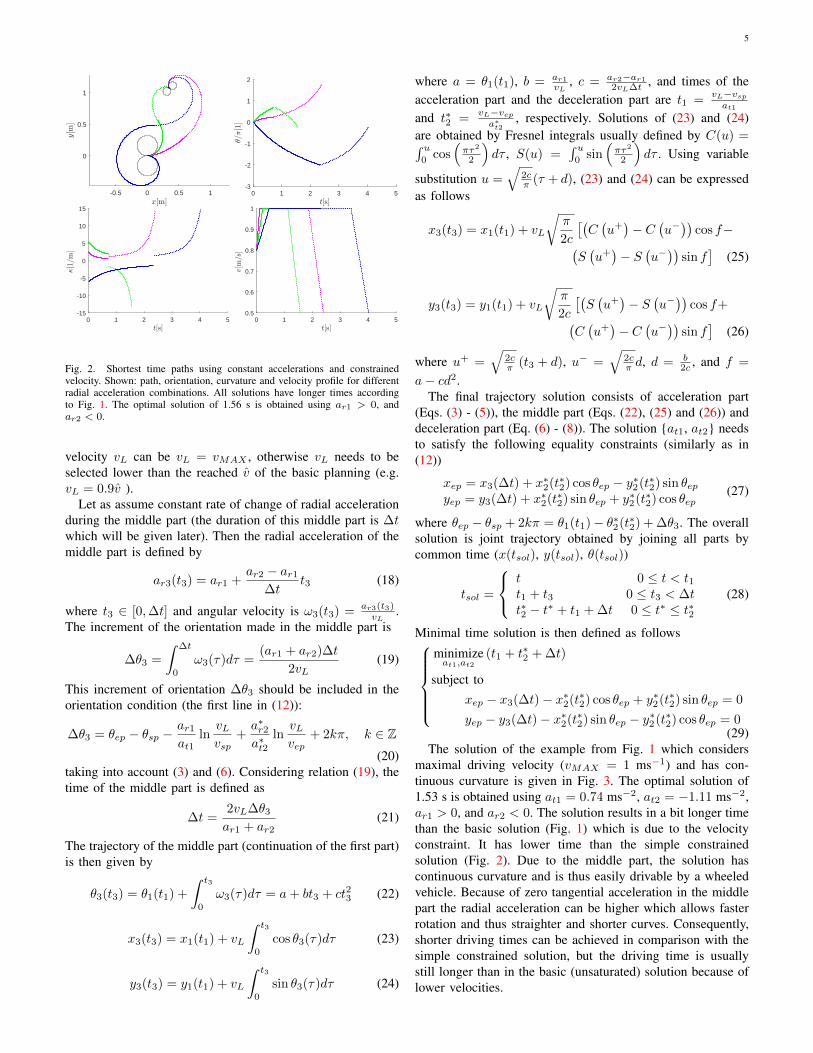
The solution of the example from Fig. 1 which considersmaximal driving velocity (vMAX = 1 ms−1) and has con-tinuous curvature is given in Fig. 3. The optimal solution of1.53 s is obtained using at1 = 0.74 ms−2, at2 = −1.11 ms−2,ar1 > 0, and ar2 < 0. The solution results in a bit longer timethan the basic solution (Fig. 1) which is due to the velocityconstraint. It has lower time than the simple constrainedsolution (Fig. 2). Due to the middle part, the solution hascontinuous curvature and is thus easily drivable by a wheeledvehicle. Because of zero tangential acceleration in the middlepart the radial acceleration can be higher which allows fasterrotation and thus straighter and shorter curves. Consequently,shorter driving times can be achieved in comparison with thesimple constrained solution, but the driving time is usuallystill longer than in the basic (unsaturated) solution because oflower velocities.

6

-0.5 0 0.5 1 1.5

0

0.5

1

1.5

0 1 2 3 4 5-2

-1

0

1

2

0 1 2 3 4 5-15

-10

-5

0

5

10

15

0 1 2 3 4 50.5

0.6

0.7

0.8

0.9

1

Fig. 3. Continuous curvature shortest time paths using constant accelerationsconsidering constrained velocity. Shown: path, orientation, curvature andvelocity profile for different radial acceleration combinations. The optimalsolution of 1.53 s is obtained using ar1 > 0 and ar2 < 0.

E. Convergence analysis

To answer the question how difficult is to find the solutionby optimization, the convergence properties of the algorithmare analyzed. This is done by adopting an unconstrainedoptimization algorithm (Nelder-Mead simplex direct searchmethod in our case) where the cost function quantifies thesquared Euclidean distance D of the equality constraints vio-lation. Equality constraints from (15) are therefore transformedinto cost function:

D = (xep − x1(t1)− x∗2(t∗2) cos θep + y∗2(t∗2) sin θep)2

+

(yep − y1(t1)− x∗2(t∗2) sin θep − y∗2(t∗2) cos θep)2 (30)

The proposed CACD solutions will be analysed by showingthe cost function D with respect to the free parameters at1and at2. The equality constraints from (15) are satisfied whenthe cost function (30) becomes zero. There can be severalsolutions but we are only interested in finding the one thatcorresponds to the minimum driving time.

Fig. 4 shows the cost function D for the example in Fig. 1with ar1 > 0 and ar2 > 0 (magenta line with travel time 1.9s in Fig. 1). Only one point (at1 = 1.81 ms−2, at2 = −0.94ms−2) satisfies the constraints and its optimal travelling timefound using (15) is 1.9 s. Because of convex cost function thissolution is found easily.

Fig. 5 shows the quadratic Euclidean distance of constraintsviolation for the example in Fig. 1 with ar1 > 0 and ar2 < 0(green line in Fig. 1). Here more points satisfy the constraintsand they all present valid trajectories, constraint optimizationthus returns the one with minimal time which is 1.42 s (atat1 = 0.90 ms−2, at2 = −1.14 ms−2). In Fig. 5 the optimalsolution (fastest trajectory) is marked by a dot. Other validtrajectories (not with minimal time) belong to lower tangentialaccelerations and higher radial accelerations and can thereforehave several encirclement of the start or the end point. Some

Fig. 4. Squared Euclidean distance of equality constraint violation for ar1 >0 and ar2 > 0 in Fig. 1. Optimal solution of (15) is therefore found atat1 = 1.81 ms−2, at2 = −0.94 ms−2 with travelling time of 1.9 s.

TABLE IVALID TRAJECTORY’S PARAMETERS AND THEIR TRAVELLING TIMES

OBTAINED FOR EXAMPLE IN FIG. 1 WITH ar1 > 0 AND ar2 < 0.

time [s] at1 [ms−2] −at2 [ms−2]

1.42 0.905 1.1374.47 0.235 0.4037.47 0.137 0.246

10.47 0.097 0.17713.47 0.075 0.13816.46 0.062 0.11019.46 0.053 0.091

......

...

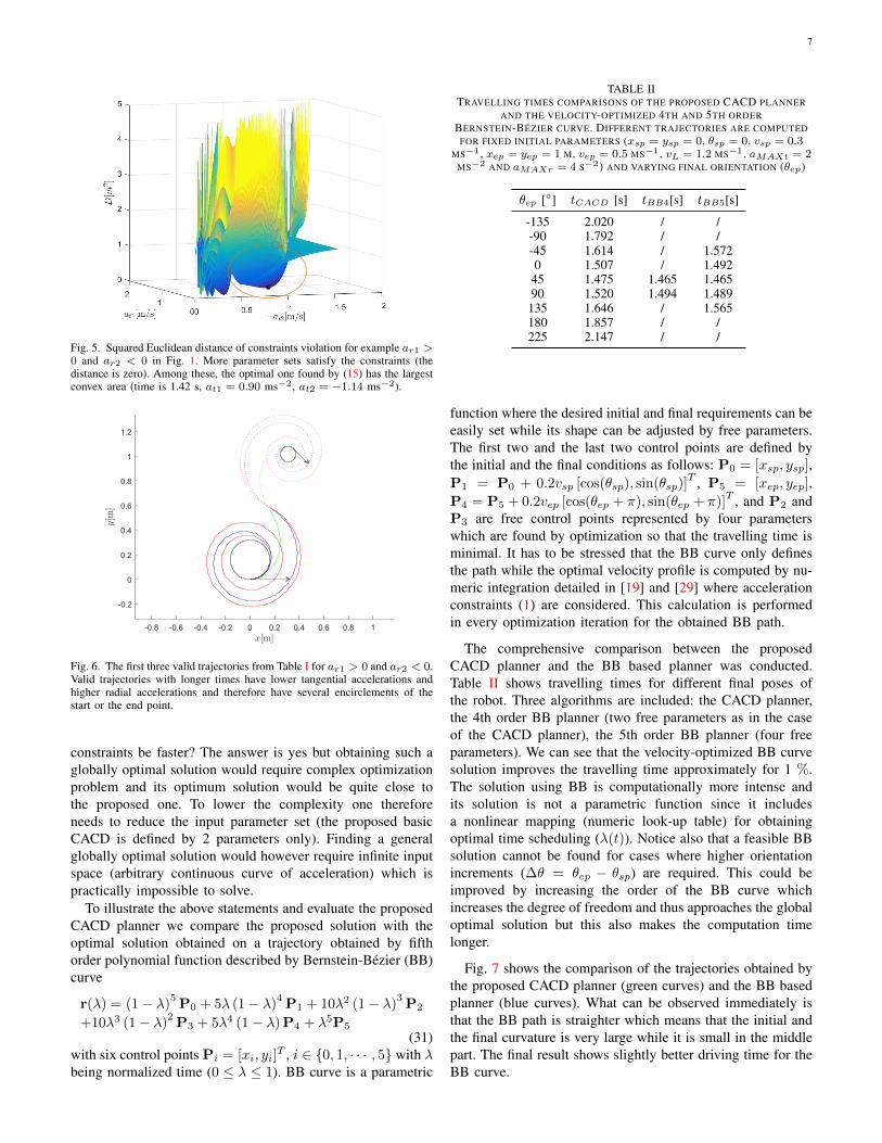
of those trajectories given in ascending order of the travelingtime are given in Table I. The shape of the cost function aroundall the solutions of the constrained optimization problem (15)is convex but the size of the basin of attraction varies. Thecost function around the solutions increases more rapidly forsolutions with longer time. The solution with the shortest time(encircled in Fig. 5) has the largest basin of attraction, andtherefore it is very easy to be found which is beneficial forthe convergence of the proposed algorithm.

IV. EXAMPLES AND COMPARISONS

The obtained CACD trajectory, either the basic one (15) orthe one with continuous curvature (29), is guaranteed to betime optimal (taking into consideration the given restrictions)as this follows from the problem definition. The obtainedtrajectory gives the feasible path and at the same time itsvelocity profile on this path is already time optimal. It istherefore not possible to drive faster on the obtained path ifthe constraints (on accelerations and maximal velocity) areconsidered.

A. Comparison with Bernstein-Bézier curve

The remaining question is how close to the global optimumthe obtained path is. In other words: can a trajectory with non-constant accelerations which would still obey the mentioned

7

Fig. 5. Squared Euclidean distance of constraints violation for example ar1 >0 and ar2 < 0 in Fig. 1. More parameter sets satisfy the constraints (thedistance is zero). Among these, the optimal one found by (15) has the largestconvex area (time is 1.42 s, at1 = 0.90 ms−2, at2 = −1.14 ms−2).

Fig. 6. The first three valid trajectories from Table I for ar1 > 0 and ar2 < 0.Valid trajectories with longer times have lower tangential accelerations andhigher radial accelerations and therefore have several encirclements of thestart or the end point.

constraints be faster? The answer is yes but obtaining such aglobally optimal solution would require complex optimizationproblem and its optimum solution would be quite close tothe proposed one. To lower the complexity one thereforeneeds to reduce the input parameter set (the proposed basicCACD is defined by 2 parameters only). Finding a generalglobally optimal solution would however require infinite inputspace (arbitrary continuous curve of acceleration) which ispractically impossible to solve.

To illustrate the above statements and evaluate the proposedCACD planner we compare the proposed solution with theoptimal solution obtained on a trajectory obtained by fifthorder polynomial function described by Bernstein-Bézier (BB)curve

r(λ) = (1− λ)5P0 + 5λ (1− λ)

4P1 + 10λ2 (1− λ)

3P2

+10λ3 (1− λ)2P3 + 5λ4 (1− λ)P4 + λ5P5

(31)with six control points Pi = [xi, yi]

T , i ∈ {0, 1, · · · , 5} with λbeing normalized time (0 ≤ λ ≤ 1). BB curve is a parametric

TABLE IITRAVELLING TIMES COMPARISONS OF THE PROPOSED CACD PLANNER

AND THE VELOCITY-OPTIMIZED 4TH AND 5TH ORDERBERNSTEIN-BÉZIER CURVE. DIFFERENT TRAJECTORIES ARE COMPUTED

FOR FIXED INITIAL PARAMETERS (xsp = ysp = 0, θsp = 0, vsp = 0.3MS−1 , xep = yep = 1 M, vep = 0.5 MS−1 , vL = 1.2 MS−1 , aMAXt = 2

MS−2 AND aMAXr = 4 S−2) AND VARYING FINAL ORIENTATION (θep)

θep [◦] tCACD [s] tBB4[s] tBB5[s]

-135 2.020 / /-90 1.792 / /-45 1.614 / 1.5720 1.507 / 1.49245 1.475 1.465 1.46590 1.520 1.494 1.489

135 1.646 / 1.565180 1.857 / /225 2.147 / /

function where the desired initial and final requirements can beeasily set while its shape can be adjusted by free parameters.The first two and the last two control points are defined bythe initial and the final conditions as follows: P0 = [xsp, ysp],P1 = P0 + 0.2vsp [cos(θsp), sin(θsp)]

T , P5 = [xep, yep],P4 = P5 + 0.2vep [cos(θep + π), sin(θep + π)]

T , and P2 andP3 are free control points represented by four parameterswhich are found by optimization so that the travelling time isminimal. It has to be stressed that the BB curve only definesthe path while the optimal velocity profile is computed by nu-meric integration detailed in [19] and [29] where accelerationconstraints (1) are considered. This calculation is performedin every optimization iteration for the obtained BB path.

The comprehensive comparison between the proposedCACD planner and the BB based planner was conducted.Table II shows travelling times for different final poses ofthe robot. Three algorithms are included: the CACD planner,the 4th order BB planner (two free parameters as in the caseof the CACD planner), the 5th order BB planner (four freeparameters). We can see that the velocity-optimized BB curvesolution improves the travelling time approximately for 1 %.The solution using BB is computationally more intense andits solution is not a parametric function since it includesa nonlinear mapping (numeric look-up table) for obtainingoptimal time scheduling (λ(t)). Notice also that a feasible BBsolution cannot be found for cases where higher orientationincrements (∆θ = θep − θsp) are required. This could beimproved by increasing the order of the BB curve whichincreases the degree of freedom and thus approaches the globaloptimal solution but this also makes the computation timelonger.

Fig. 7 shows the comparison of the trajectories obtained bythe proposed CACD planner (green curves) and the BB basedplanner (blue curves). What can be observed immediately isthat the BB path is straighter which means that the initial andthe final curvature is very large while it is small in the middlepart. The final result shows slightly better driving time for theBB curve.

8

0 0.5 1

0

0.2

0.4

0.6

0.8

1

0 0.5 1 1.5 2-0.1

0

0.1

0.2

0.3

0.4

0 0.5 1 1.5 20.2

0.4

0.6

0.8

1

1.2

0 0.5 1 1.5 2-20

-10

0

10

20

30

40

0 0.5 1 1.5 2-2

-1

0

1

2

0 0.5 1 1.5 2-4

-3

-2

-1

0

1

2

3

Fig. 7. Comparison of the proposed CACD trajectory (green) and velocity-optimized Bernstein-Bézier curve (blue) for initial parameters (xsp = ysp =0, θsp = 0, vsp = 0.3 ms−1, xep = yep = 1 m, ,θep = −10◦, vep = 0.5ms−1, vL = 1.2 ms−1, aMAXt = 2 ms−2 and aMAXr = 4 s−2).

B. Illustration of other possible applications

The proposed CACD motion planner can have severalapplications. It can be used as a standalone motion plannerin obstacle free environment as illustrated in Sections III andIV-C. It can also be used as CACD motion primitive generatorin some other path planners to estimate cost-to-goal heuristicsor to build a lattice graph for environments with obstacles.It can as well be used to smooth a path defined by a set ofway-points which is obtained from some path planner. Fig.8 shows an illustration of path smoothing and lattice graphconstruction. In the upper graph in Fig. 8 the path consistingof straight-line sections (going from x = 0 m and y = 0 m tox = 2 m and y = 0 m, then to x = 0.5 m and y = 2 m, andso on) is smoothed by inserting CACD motion primitives. Thestart and the goal points of the connecting CACD curve lie at aconstant distance from the junction point of the two sequentialstraight-line segments. The start and the goal orientations aredefined by straight-line sections.

The lower graph in Fig. 8 illustrates the lattice graphconstruction using CACD motion primitives that could be usedto explore the environment in some graph-based planner. Inthis example each CACD curve starts from its parent final poseand ends in the pose with one of the orientation increments(−45◦, 0◦, 45◦).

0 1 2 3 4

0

1

2

3

4

-0.5 0 0.5 1

0

0.5

1

1.5

Fig. 8. Illustration of path smoothing application (upper graph) where thestraight-line path with discontinuous orientation in the junctions is smoothedby inserting the CACD curves (thick green line). Illustration of a lattice graphconstruction (lower graph) using CACD motion primitives where each node(final point of the CACD curve) expands to three new vertices connected bythe CACD curves.

C. Experiments

Performance of the proposed trajectory planners is checkedalso by several experiments done on a wheeled mobile robot.The robot (see Fig. 9) has a cube shape with a 7.5 cm sideand weighs 0.5 kg. Its pose is estimated with an image sensorand a computer-vision algorithm running at the samplingfrequency of 30 Hz. The robot is controlled by commandingits translational velocity (v(t)) and its angular velocity (ω(t))which present the reference for implemented low-level controlin the robot.

Trajectory tracking is achieved by nonlinear control law [30]

v(t) = vref (t) cos eθ(t) + kx(t)ex(t)

ω(t) = ωref (t) + ky(t)vref (t) sin eθ(t)eθ(t) ey(t) + kθ(t)eθ(t)

where ex(t), ey(t) and eθ(t) are the components of the posetracking error expressed in robot local coordinates, vref (t) =√x2(t) + y2(t)2 and ωref (t) = x(t)y(t)−y(t)x(t)

x2(t)+y2(t) are the refer-ence velocities computed from the planned trajectory, kx(t) =

kϕ(t) = 2ζ√ω2ref (t) + gv2

ref (t) and ky(t) = gvref (t) are thecontroller gains with tuning parameters chosen as ζ = 0.8,g = 150.

9

Fig. 9. Robot used during experiments with the color patch used for vision-based localization.

The algorithms treated in this comparison are the basicCACD trajectory planning algorithm with limited maximalvelocity (Section III-C) and the CACD trajectory planning al-gorithm with continuous curvature transitions (Section III-D).

Both planning approaches result in minimal time path undergiven design constraints (maximal velocity and accelerations).The basic CACD results in an angular velocity with a dis-continuity (due to discontinuous curvature). This sudden jumpinfluences the final tracking performance but it can also behidden by other prevailing effects such as tracking controllerdynamics, relatively long sampling time (Ts = 33 ms),measurement system delay (in our case approximately 2Tsdue to localization using image sensor), unmodelled dynamics,wheel sliding and noise.

Experiments on the real mobile robot are shown Fig.10. The first two plots show the x, y plot together withtheir references, next two plots show the actual velocitiesand the commanded velocities while the last plot showsthe position error between planned trajectory (x(t), y(t))and robot trajectory (xrob(t), yrob(t)) defined as: derr(t) =√

(x(t)− xrob(t))2 + (y(t)− yrob(t))2. In the experiment inFig. 10 maximal accelerations are selected so the robot canstill reliably track the trajectory most of the time. The mainpurpose of the experiments is to show that both planners canprovide similar reference trajectories with similar travelingtimes (tCACD = 3.56 s, tCκ−CACD = 3.63 s) if observingthe paths in Fig. 10. However, due to discontinuity in thecurvature present in the basic CACD planner, the requiredangular velocity needs to make sudden change which causeslarger tracking error as seen in Fig. 10. The controller mayneed some more time to recover from this error if robot isdriving with accelerations on the edge of slipping. This effectof discontinuity in curvature becomes noticeable at jump ofthe angular velocity in the basic CACD (after 1.6 s).

V. CONCLUSION

In this work, a novel trajectory planning algorithm isproposed to generate minimal time trajectories for wheeledmobile robots. The solution is found for given initial andfinal configurations considering driving constraints on max-imal velocity and accelerations. The proposed solutions are

0.2 0.4 0.6 0.8 1 1.20.2

0.4

0.6

0.8

1

1.2

refC -CACD

0.2 0.4 0.6 0.8 1 1.20.2

0.4

0.6

0.8

1

1.2

refCACD

0 1 2 3 4-3

-2

-1

0

1

2

3

4

ref v (C -CACD)ref (C -CACD)v (C -CACD)

(C -CACD)

0 1 2 3 4-2

-1

0

1

2

3

ref v (CACD)ref (CACD)v (CACD)

(CACD)

0 1 2 3 40

0.005

0.01

0.015

0.02

C -CACDCACD

Fig. 10. Comparison of continuous curvature CACD (Cκ-CACD) and basicCACD tracking results. Trajectories parameters are: xsp = ysp = 0, θsp = 0,vsp = 0.1 ms−1, xep = 1.3 m yep = 1.2 m, θep = −10◦, vep = 0.2ms−1, vL = 0.5 ms−1, aMAXt = 0.5 ms−2, aMAXr = 0.5 s−2.

derived analytically for constant-acceleration and constant-deceleration motion. In the basic solution the resulting CACDtrajectory is a compact parametric function parametrized bytwo parameters only, i.e. maximal acceleration and maximaldeceleration. These parameters are obtained by constrainedoptimization which solves two equations for the two unknownparameters. Minimal time solution is easily found as shownin the provided convergence analysis.

To achieve feasible trajectories which vehicles can easilydrive on, the basic solution is extended to obtain continuoustransitions of curvature. The basic solution and its modificationwith considered maximal driving velocity (Section III-B andIII-C) guarantee optimal trajectory in the sense of travelingtime. The solution given in Section III-D results in a continu-ous curvature trajectory whose traveling time is in the majorityof cases even shorter than in solution from Section III-C. Thisis possible because the inserted path section allows faster robotrotation and consequently straighter and shorter accelerationand deceleration parts. Note that the proposed approach doesnot only optimize the velocity profile for a given path butinstead adapts trajectory to obtain minimal time. This allows tocompensate for the lost time due to the included modificationby path corrections. The obtained solution is optimal for thedefined function in the middle curve part but there may exista better function.

The proposed solutions are evaluated by several path-planning examples and by a comparison to the planner using

10

Bernstein-Bezier curves with applied additional velocity op-timization. It is shown that CACD planner provides compu-tationally efficient and time optimal solutions using constant-acceleration and constant-deceleration motion and consideringthe mentioned driving constraints. As such it can be appliedin path smoothing and path planning applications as a stand-alone planner in unobstructed environments or as a motionprimitive generator in lattice-graph based search planners inthe presence of static or dynamic obstacles.

REFERENCES

[1] T. Fraichard and A. Scheuer, “From reeds and shepp’s to continuous-curvature paths,” IEEE Transactions on Robotics, vol. 20, no. 6, pp.1025–1035, 2004.

[2] J. Choi and K. Huhtala, “Constrained global path optimization for artic-ulated steering vehicles,” IEEE Transactions on Vehicular Technology,vol. 65, no. 4, pp. 1868–1879, April 2016.

[3] D. J. Webb and J. van den Berg, “Kinodynamic RRT*: Asymptoticallyoptimal motion planning for robots with linear dynamics,” in 2013 IEEEInternational Conference on Robotics and Automation (ICRA), 2013, pp.5054–5061.

[4] A. Piazzi, C. G. L. Bianco, and M. Romano, “ η3-splines for thesmooth path generation of wheeled mobile robots,” IEEE Transactionson Robotics, vol. 3, no. 53, pp. 1089–1095, 2007.

[5] D. Dolgov, S. Thrun, M. Montemerlo, and J. Diebel, “Path planning forautonomous vehicles in unknown semi-structured environments,” TheInternational Journal of Robotics Research, vol. 29, no. 5, pp. 485–501, 2010.

[6] M. Likhachev and D. Ferguson, “Planning long dynamically-feasiblemaneuvers for autonomous vehicles,” The International Journal ofRobotics Research, vol. 28, no. 8, pp. 933–945, 2009.

[7] M. Pivtoraiko, R. Knepper, and A. Kelly, “ Differentially constrainedmobile robot motion planning in state lattices,” Robotics and Au-tonomous Systems, vol. 26, no. 3, pp. 308–333, 2009.

[8] L. Dubins, “On curves of minimal length with a constraint on averagecurvature and with prescribed initial and terminal positions and tan-gents,” Amer. J. Math., vol. 79, pp. 497–516, 1957.

[9] J. A. Reeds and L. A. Shepp, “Optimal paths for a car that goes bothforwards and backwards.” Pacific J. Math., vol. 145, no. 2, pp. 367–393,1990.

[10] P. Soueres and J. P. Laumond, “Shortest paths synthesis for a car-likerobot,” IEEE Transactions on Automatic Control, vol. 41, no. 5, pp.672–688, May 1996.

[11] P. Salaris, D. Fontanelli, L. Pallottino, and A. Bicchi, “Shortest pathsfor a robot with nonholonomic and field-of-view constraints,” IEEETransactions on Robotics, vol. 26, no. 2, pp. 269–281, April 2010.

[12] S. Fallah, B. Yue, O. Vahid-Araghi, and A. Khajepour, “Energy man-agement of planetary rovers using a fast feature-based path planningand hardware-in-the-loop experiments,” IEEE Transactions on VehicularTechnology, vol. 62, no. 6, pp. 2389–2401, July 2013.

[13] J. Yang, L. Chou, and Y. Chang, “Electric-vehicle navigation systembased on power consumption,” IEEE Transactions on Vehicular Tech-nology, vol. 65, no. 8, pp. 5930–5943, Aug 2016.

[14] J.-W. Choi, R. Curry, and G. Elkaim, Machine Learning and SystemsEngineering, ser. Lecture Notes in Electrical Engineering 68. SpringerScience+Business Media, 2010, ch. Piecewise Bezier Curves Path Plan-ning with Continuous Curvature Constraint for Autonomous Driving,pp. 31–45.

[15] M. Brezak and I. Petrovic, “Real-time approximation of clothoids withbounded error for path planning applications,” IEEE Transactions onRobotics, vol. 30, no. 2, pp. 507–515, April 2014.

[16] B. Sencer, K. Ishizaki, and E. Shamoto, “A curvature optimal sharpcorner smoothing algorithm for high-speed feed motion generation ofNC systems along linear tool paths,” International Journal of AdvancedManufacturing Technology, vol. 76, no. 9, pp. 1977–1992, 2015.

[17] F. Ghilardelli, L. Gabriele, and A. Piazzi, “Path Generation Usingη4-Splines for a Truck and Trailer Vehicle,” IEEE Transactions onAutomation Science and Engineering, vol. 11, no. 1, pp. 187–203, 2014.

[18] E. Velenis and P. Tsiotras, “Minimum-time travel for a vehicle withacceleration limits: Theoretical analysis and receding-horizon implemen-tation,” Journal of Optimization Theory and Applications, vol. 138, no. 2,pp. 275–296, Aug 2008.

[19] M. Lepetic, G. Klancar, I. Škrjanc, D. Matko, and B. Potocnik, “Timeoptimal path planning considering acceleration limits,” Robotics andAutonomous Systems, vol. 45, pp. 199–210, 2003.

[20] Q.-C. Pham, S. Caron, P. Lertkultanon, and Y. Nakamura, “Admissi-ble velocity propagation: Beyond quasi-static path planning for high-dimensional robots,” The International Journal of Robotics Research,vol. 36, no. 1, pp. 44–67, 2017.

[21] A. Zdešar and I. Škrjanc, “Optimum velocity profile of multiplebernstein-bezier curves subject to constraints for mobile robots,” ACMTrans. Intell. Syst. Technol., vol. 9, no. 5, pp. 56:1–56:23, 2018.

[22] D. J. Balkcom and M. T. Mason, “Time optimal trajectories forbounded velocity differential drive vehicles,” The International Journalof Robotics Research, vol. 21, no. 3, pp. 199–217, 2002.

[23] M. Renaud and J. Y. Fourquet, “Minimum time motion of a mobilerobot with two independent, acceleration-driven wheels,” in Proceedingsof International Conference on Robotics and Automation, vol. 3, 1997,pp. 260–2613.

[24] H. Wang, Y. Chen, and P. Soueres, “A geometric algorithm to com-pute time-optimal trajectories for a bidirectional steered robot,” IEEETransactions on Robotics, vol. 25, no. 2, pp. 399–413, April 2009.

[25] D. B. Reister and F. G. Pin, “Time-optimal trajectories for mobile robotswith two independently driven wheels,” The International Journal ofRobotics Research, vol. 13, no. 1, pp. 38–54, 1994.

[26] S. Fleury, P. Soueres, J.-P. Laumond, and R. Chatila, “Primitives forsmoothing mobile robot trajectories,” IEEE Transactions on Roboticsand Automation, vol. 11, no. 3, pp. 441–448, 1995.

[27] S. Yoon, D. Lee, J. Jung, and D. H. Shim, “Spline-based RRT* usingpiecewise continuous collision-checking algorithm for car-like vehicles,”Journal of Intelligent & Robotic Systems, pp. 1–13, 2017.

[28] G. Tanzmeister, D. Wollherr, and M. Buss, “Grid-based multi-road-course estimation using motion planning,” IEEE Transactions on Ve-hicular Technology, vol. 65, no. 4, pp. 1924–1935, April 2016.

[29] G. Klancar, A. Zdešar, S. Blažic, and I. Škrjanc, Wheeled mobilerobotics - From fundamentals towards autonomous systems. Elsevier,Butterworth-Heinemann, 2017.

[30] C. Samson, “Time-varying Feedback Stabilization of Car-like WheeledMobile Robots,” International Journal of Robotics Research, vol. 12,no. 1, pp. 55–64, 1993.

Gregor Klancar received B.Sc. and Ph.D. degreesin electrical engineering from the University ofLjubljana, Faculty of Electrical Engineering, Slove-nia, in 1999 and 2003 respectively.

He is currently an Associate Professor with theFaculty of Electrical Engineering, University ofLjubljana. He lectures autonomous mobile systemsat graduate and advanced control of autonomoussystems at postgraduate study. His current researchinterests include autonomous mobile robots, motioncontrol, trajectory tracking, path planning, localiza-

tion, agent-based behaviour systems and supervision of multiagent systems.

Sašo Blažic received the B.Sc., M. Sc., and Ph. D.degrees in 1996, 1999, and 2002, respectively, fromthe University of Ljubljana, Faculty of ElectricalEngineering, Slovenia.

He is currently a Professor with the University ofLjubljana, Faculty of Electrical Engineering. From2017, he holds the position of the Vice-Dean for Re-search at the Faculty of Electrical Engineering, Uni-versity of Ljubljana. His research interests includeadaptive, fuzzy and predictive control of dynamicalsystems, modelling of nonlinear and evolving sys-

tems, autonomous mobile systems, trajectory tracking and path planning ofwheeled mobile robots.