optimal location of interline power flow controller in a...

ARCHIVES OF ELECTRICAL ENGINEERING VOL. 62(1), pp. 91-110 (2013)

DOI 10.2478/aee-2013-0007

Optimal location of interline power flow controller in a power system network using ABC algorithm

S. SREEJITH, SISHAJ PSIMON, M.P. SELVAN

Department of Electrical and Electronics Engineering

National Institute of Technology, Trichy-15, India e-mail: [email protected], {sishajpsimon / selvanmp}@nitt.edu

(Received: 31.01.2012, revised: 05.11.2012)

Abstract: This paper proposes a methodology based on installation cost for locating the optimal position of interline power flow controller (IPFC) in a power system network. Here both conventional and non conventional optimization tools such as LR and ABC are applied. This methodology is formulated mathematically based on installation cost of the FACTS device and active power generation cost. The capability of IPFC to control the real and reactive power simultaneously in multiple transmission lines is exploited here. Apart from locating the optimal position of IPFC, this algorithm is used to find the optimal dispatch of the generating units and the optimal value of IPFC parameters. IPFC is modeled using Power Injection (PI) model and incorporated into the problem formula-tion. This proposed method is compared with that of conventional LR method by validat-ing on standard test systems like 5-bus, IEEE 30-bus and IEEE 118-bus systems. A de-tailed discussion on power flow and voltage profile improvement is carried out which reveals that incorporating IPFC into power system network in its optimal location signi-ficantly enhance the load margin as well as the reliability of the system. Key words: IPFC, power injection model, power flow control, ABC algorithm, cost minimization

1. Introduction The main purpose of transmission network is to supply the load at the required reliability, lower cost and with maximum efficiency. The complexity of the power system is increasing due to the increase in load demand, line loss and loop flows. Increasing the power generation and constructing new transmission lines are essential for meeting this load demand. The cost of transmission lines, social and geographical factors, financial factors and ambient factors restrict the construction of new lines to improve the transmission capability. The best solutions available for sorting out this problem are HVDC and FACTS. HVDC is economical only for long distance transmission. The available transmission capability can be increased to a certain level using FACTS by utilizing the existing transmission lines. FACTS devices can control the various parameters of the power system such as voltage, phase angle and line impedance in a rapid and effective manner.

Unauthenticated | 89.67.242.59Download Date | 5/12/13 6:28 PM

S. Sreejith, S. Psimon, M.P. Selvan Arch. Elect. Eng. 92

FACTS devices can be categorized as switch based controllers and converter based cont-rollers, which can be further classified as shunt, series and combination of shunt and series controllers. FACTS devices include Static Var Compensator (SVC), Thyristor Controlled Se-ries Compensator (TCSC), Static Series Synchronous Compensator (SSSC), Static Compen-sator (STATCOM), Unified Power Flow Controller (UPFC) and Interline Power Flow Cont-roller (IPFC) [1, 2]. These devices can be used depending on requirements and applications. UPFC is used to control three variables namely real power, reactive power and voltage control simultaneously or as required. IPFC is used to control the real and reactive power flow in multiple transmission lines simultaneously. But taking advantages of these FACTS devices depends greatly on how these devices are placed in the network (i.e) the location of the device [17]. Improperly placed FACTS devices fail to provide the optimum performance and can be counterproductive in certain situations. So, proper placement of these FACTS devices is an important task. However, the best choice of location for the installation of these equipments is not a simple task due to the complexity of the electric system. The main objective of Optimal Power Flow (OPF) is to determine the optimal operation state of the power system subjected to certain operating constraints. OPF is carried out before locating the optimal position of a FACTS device. Using PSO technique the optimal location of FACTS devices (SVC, TCSC and UPFC) is carried out in [3]. The mathematical model repre-sentations of variable series capacitors and static phase shifters to find the optimal location for improved economic dispatch has been developed by Tjing T Lie and Wanhong Deng [4]. The optimal choice and allocation of FACTS devices (UPFC, TCSC, TCPST, and SVC) are done in a multi machine power system using Genetic Algorithm (GA) is given in [5]. In [6], optimal location and the parameter settings for UPFC are carried out using PSO AND GA for improv-ing the loadability of the power system. In [7], optimal location for SVC and TCSC are carried out using CP flow analysis, to enhance the voltage stability of the system. The optimal place-ment of FACTS devices (TCSC, STATOM, UPFC) in a deregulated power system with due consideration to line loss is being discussed in [8]. In reference [9] optimal power flow using ABC algorithm which is developed by Karaboga D and Basturk B [10] is carried out. Teerathana.S [9] applied successive quadratic algorithm to solve the OPF incorporating IPFC in the network with an objective to reduce total capacity of installed IPFC in a power system. Khalid. H. Mohamed [10] had solved OPF problem incorporating IPFC using PSO, GA and SA, with an objective to reduce the real power loss in the network. Basu [11] proposed an algorithm based on Differential Evolution approach to solve optimal power flow problem incorporating TCSC, TCPS and obtained better results in case of fuel cost and CPU timing. 1.1. Proposed work

The focus of this work is to locate the optimal position for IPFC in a given test system using ABC algorithm while satisfying all the operating and IPFC constraints. The minimi-zation of line loss, economic dispatch of generators, improve power flow and reduction in the overall system cost which includes the cost of active power generation and the installation cost of IPFC are also considered for obtaining the optimal location. Since the selected line is compensated, this will lead to the reduction in total generation cost of electric power and


Vol. 62(2013) Optimal location of IPFC using ABC algorithm 93

investment on the compensating devices. Limited works has been carried out in optimizing the power flow in a power system network with IPFC and optimal location of IPFC. The cost function for IPFC is derived from the existing UPFC cost function with an assumption that there is not much difference in the construction of UPFC and IPFC. In [10], it is clearly proven that ABC algorithm can be efficiently used for solving constrained optimization prob-lems. The convergence characteristic of ABC is also better, so in this proposed methodology ABC algorithm is used as an optimization tool. The developed methodology is tested in standard test systems such as 5 bus, IEEE 30 bus and IEEE 118 bus systems.

2. Interline power flow controller 2.1. Operating principle and mathematical modeling

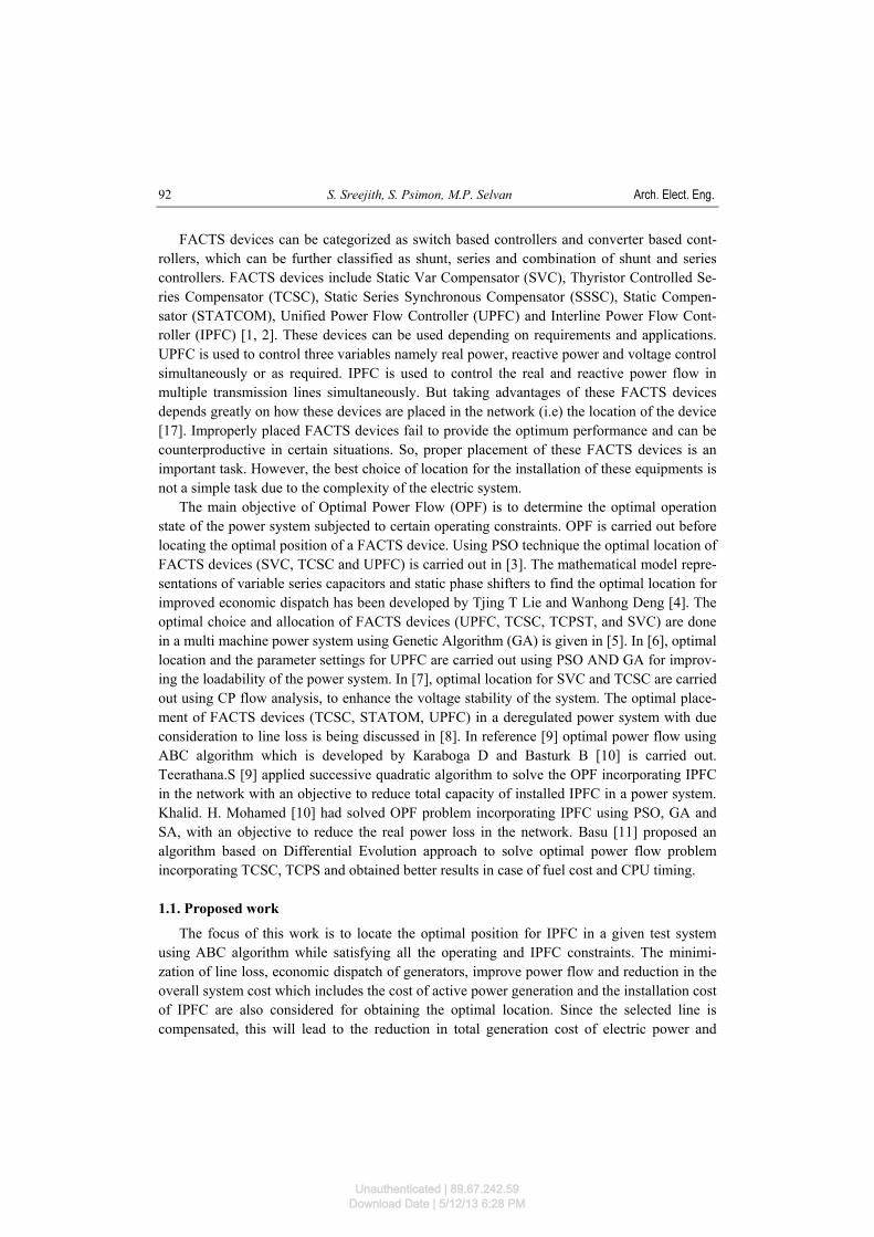
The IPFC addresses the problem of compensating a number of transmission lines at a given substation. Conventionally series capacitors are used to improve the real power tran-sfer in a given line. However, it cannot control the reactive flow in the line, thus resulting in improper compensation. This problem occurs when the ratio of reactance to resistance of transmission line (X/R) is relatively low. By using capacitive combination, the reactance of the line decreases which in turn reduces the (X/R) ratio of the line, resulting in improper com-pensation and improper load balancing in transmission lines. Series reactive compensation reduces only the effective reactive impedance X and, thus, significantly decreases the effective X/R ratio and thereby increases the reactive power flow and losses in the line. The IPFC scheme, together with independently controllable reactive series compensation of each indivi-dual line enables the transfer of real power between the compensated lines. IPFC can be em-ployed to transfer power between multiple lines in a substation, where as the other available FACTS devices can control the power flow through single line only. The power flow through a line can be regulated by controlling both magnitudes and angles of the series voltage in-jections. The converters have the capability of independently generating or absorbing the reactive power.

Fig. 1. Schematic diagram of IPFC



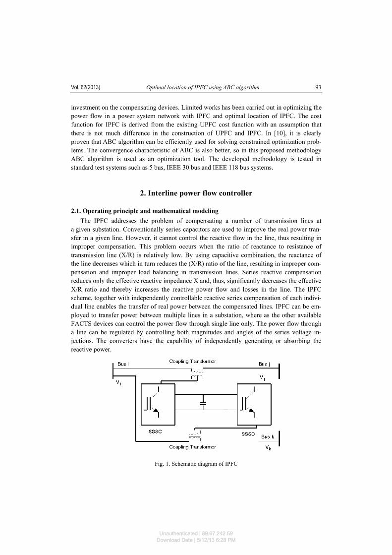
Mathematical model for IPFC, which will be referred to as power injection model, is helpful in understanding the impact of the IPFC on the power system in the steady state. Furthermore, this IPFC model can easily be incorporated in power flow analysis. Usually, in the steady state analysis of power system, the Voltage Source Converters (VSC) may be re-presented as a synchronous voltage source [15, 16, 19] injecting an almost sinusoidal voltage with controllable magnitude and angle [5].

Fig. 2. Equivalent circuit of IPFC Based on Figure 1, the equivalent circuit of IPFC is shown in Figure 2. In Figure 2, Vi, Vj and Vk are the complex bus voltages at the buses i, j and k respectively, Vsein is the complex controllable series injected voltage source, and Zsein (n = j, k) is the series coupling trans-former impedance. The complex power injected by series converter connected in between bus i and bus j as shown in Figure 2 can be written as

( )

( ) ( )( ),sincos

sincos

1

1

2

ijseijijijseijij

n

i,jjijsei

ijijijij

n

i,jjjiiiii

θθbθθgVV

θbθgVVgVP

−−−+

−−−=

∑

∑

≠=

≠= (1)

( )

( ) ( )( ),cossin

cossin

1

1

2

∑

∑

≠=

≠=

−−−+

−−−=

n

i,jjijijijijijijiji

n

i,jjijijijijjiiiii

seθθbseθθgVseV

θbθgVVbVQ

(2)



( ) ( )( )

( ) ( )( ),sincos

sincos

1

1

2

ijseijijijseijij

n

i,jjijsei

ijijijijij

n

i,jjjiiijji

θθbθθgVV

θθbθθgVVgVP

−−−+

−−−−−=

∑

∑

≠=

≠= (3)

( ) ( )( )

( ) ( )( ),cossin

cossin

1

1

2

ijseijijijseijij

n

i,jjijsei

ijijijijij

n

i,jjjiiijji

θθbθθgVV

θθbθθgVVgVQ

−−−+

−−−−−=

∑

∑

≠=

≠= (4)

where:

( )

( ).Zse/1Im

,Zse/1Re

ijijii

jijii

bb

gg

=−=

=−= ι

The active power exchange between series connected inverters via the common dc link is

( ).Re1∑

≠=

=n

i,jj

*ijijmn I*VseP (5)

The same equations can be derived for bus k also.

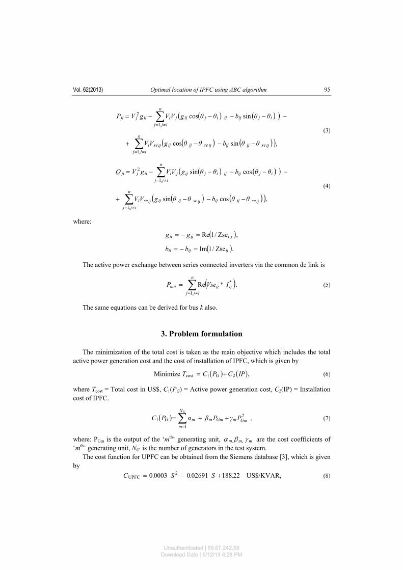
3. Problem formulation The minimization of the total cost is taken as the main objective which includes the total active power generation cost and the cost of installation of IPFC, which is given by

( ) ( ),Minimize 21cost IPCPCT G += (6)

where Tcost = Total cost in US$, C1(PG) = Active power generation cost, C2(IP) = Installation cost of IPFC.

( ) ,PγPβαPC GmmGmm

N

mmG

G2

11 ++= ∑

=

(7)

where: PGm is the output of the ‘mth’ generating unit, mmm γβα ,, are the cost coefficients of ‘mth’ generating unit, NG is the number of generators in the test system. The cost function for UPFC can be obtained from the Siemens database [3], which is given by 2218802691000030 2

UPFC .S.S.C +−= US$/KVAR, (8)



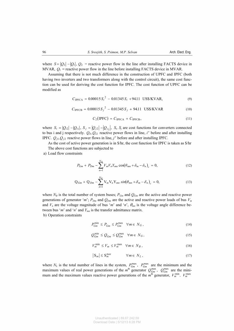
where ,12 QQS −= 2Q = reactive power flow in the line after installing FACTS device in MVAR, 1Q = reactive power flow in the line before installing FACTS device in MVAR. Assuming that there is not much difference in the construction of UPFC and IPFC (both having two inverters and two transformers along with the control circuit), the same cost func-tion can be used for deriving the cost function for IPFC. The cost function of UPFC can be modified as

1194013450000150 2IPFCA .S.S.C ii +−= US$/KVAR, (9)

1194013450000150 2IPFCB .S.S.C jj +−= US$/KVAR (10)

( ) ,IPFC IPFCBIPFCA2 CCC += (11)

where ,12 iii QQS −= ,12 jjj QQS −= Si, Sj are cost functions for converters connected to bus i and j respectively. 21 ii ,QQ reactive power flows in line, iO before and after installing IPFC. 21 jj ,QQ reactive power flows in line, jO before and after installing IPFC. As the cost of active power generation is in $/hr, the cost function for IPFC is taken as $/hr The above cost functions are subjected to a) Load flow constraints

( ) ,0cos1

=−+−+ ∑=

cnmmn

N

nmnnmDmGm δδθYVVPP

B

(12)

( ) ,0YVVQQ1

=−+−+ ∑=

cnmmn

N

nmnnmDmGm sin

B

δδθ (13)

where NB is the total number of system buses; PGm and QGm are the active and reactive power generations of generator ‘m’; PDm and QDm are the active and reactive power loads of bus Vm and Vn are the voltage magnitude of bus ‘m’ and ‘n’, 2mn is the voltage angle difference be-tween bus ‘m’ and ‘n’ and Ymn is the transfer admittance matrix. b) Operation constraints

GGmGmGm NmPPP ∈∀≤≤ maxmin , (14)

GGmGmGm NmQQQ ∈∀≤≤ maxmin , (15)

Bmmm NmVVV ∈∀≤≤ maxmin , (16)

Lmaxmm Nm ∈∀≤ SS , (17)

where NL is the total number of lines in the system, ,maxGmP max

GmP are the minimum and the maximum values of real power generations of the mth generator ,max

GmQ maxGmQ are the mini-

mum and the maximum values reactive power generations of the mth generator, ,Vmmin max

mV



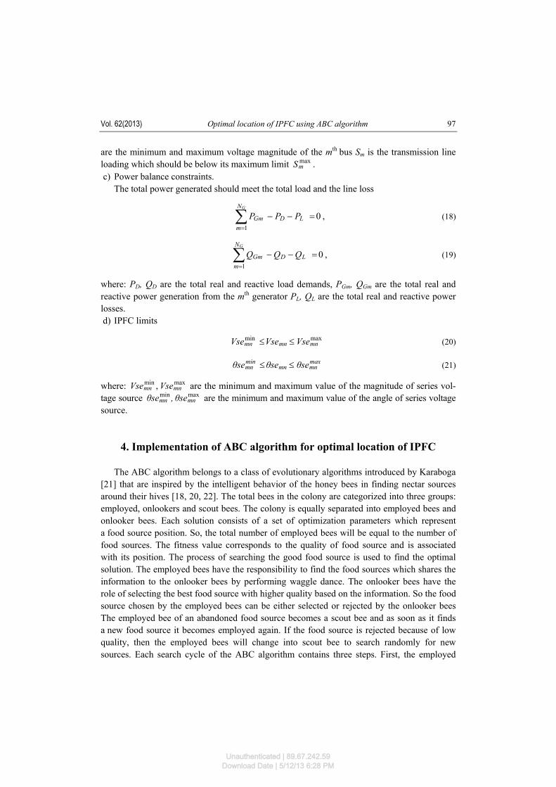
are the minimum and maximum voltage magnitude of the mth bus Sm is the transmission line loading which should be below its maximum limit max

mS . c) Power balance constraints. The total power generated should meet the total load and the line loss

,01∑=

=−−GN

mLDGm PPP (18)

,01∑=

=−−GN

mLDGm QQQ (19)

where: PD, QD are the total real and reactive load demands, PGm, QGm are the total real and reactive power generation from the mth generator PL, QL are the total real and reactive power losses. d) IPFC limits

maxminmnmnmn VseVseVse ≤≤ (20)

maxmnmn

minmn θseθseθse ≤≤ (21)

where: maxmin , mnmn VseVse are the minimum and maximum value of the magnitude of series vol-tage source maxmin

mnmn θse,θse are the minimum and maximum value of the angle of series voltage source.

4. Implementation of ABC algorithm for optimal location of IPFC The ABC algorithm belongs to a class of evolutionary algorithms introduced by Karaboga [21] that are inspired by the intelligent behavior of the honey bees in finding nectar sources around their hives [18, 20, 22]. The total bees in the colony are categorized into three groups: employed, onlookers and scout bees. The colony is equally separated into employed bees and onlooker bees. Each solution consists of a set of optimization parameters which represent a food source position. So, the total number of employed bees will be equal to the number of food sources. The fitness value corresponds to the quality of food source and is associated with its position. The process of searching the good food source is used to find the optimal solution. The employed bees have the responsibility to find the food sources which shares the information to the onlooker bees by performing waggle dance. The onlooker bees have the role of selecting the best food source with higher quality based on the information. So the food source chosen by the employed bees can be either selected or rejected by the onlooker bees The employed bee of an abandoned food source becomes a scout bee and as soon as it finds a new food source it becomes employed again. If the food source is rejected because of low quality, then the employed bees will change into scout bee to search randomly for new sources. Each search cycle of the ABC algorithm contains three steps. First, the employed



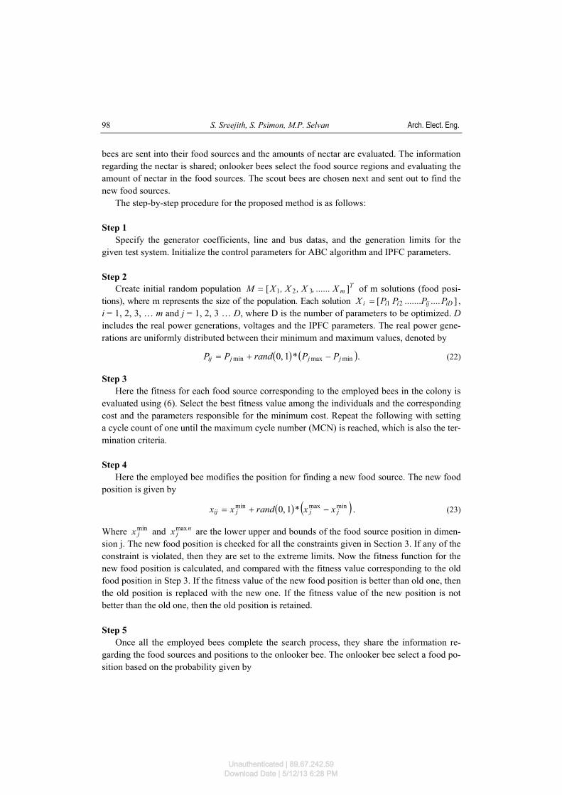
bees are sent into their food sources and the amounts of nectar are evaluated. The information regarding the nectar is shared; onlooker bees select the food source regions and evaluating the amount of nectar in the food sources. The scout bees are chosen next and sent out to find the new food sources. The step-by-step procedure for the proposed method is as follows: Step 1 Specify the generator coefficients, line and bus datas, and the generation limits for the given test system. Initialize the control parameters for ABC algorithm and IPFC parameters. Step 2 Create initial random population T

mX......,X,X,XM ][ 321= of m solutions (food posi-tions), where m represents the size of the population. Each solution ]...........[ 21 iDijiii PPPPX = , i = 1, 2, 3, … m and j = 1, 2, 3 … D, where D is the number of parameters to be optimized. D includes the real power generations, voltages and the IPFC parameters. The real power gene-rations are uniformly distributed between their minimum and maximum values, denoted by

( ) ( ).*1,0 minmaxmin jjjij PPrandPP −+= (22)

Step 3 Here the fitness for each food source corresponding to the employed bees in the colony is evaluated using (6). Select the best fitness value among the individuals and the corresponding cost and the parameters responsible for the minimum cost. Repeat the following with setting a cycle count of one until the maximum cycle number (MCN) is reached, which is also the ter-mination criteria. Step 4 Here the employed bee modifies the position for finding a new food source. The new food position is given by

( ) ( )minmaxmin *1,0 jjjij xxrandxx −+= . (23)

Where minjx and n

jxmax are the lower upper and bounds of the food source position in dimen-sion j. The new food position is checked for all the constraints given in Section 3. If any of the constraint is violated, then they are set to the extreme limits. Now the fitness function for the new food position is calculated, and compared with the fitness value corresponding to the old food position in Step 3. If the fitness value of the new food position is better than old one, then the old position is replaced with the new one. If the fitness value of the new position is not better than the old one, then the old position is retained. Step 5 Once all the employed bees complete the search process, they share the information re-garding the food sources and positions to the onlooker bee. The onlooker bee select a food po-sition based on the probability given by



∑−

= D

nn

ii

fit

fitP

1

. (24)

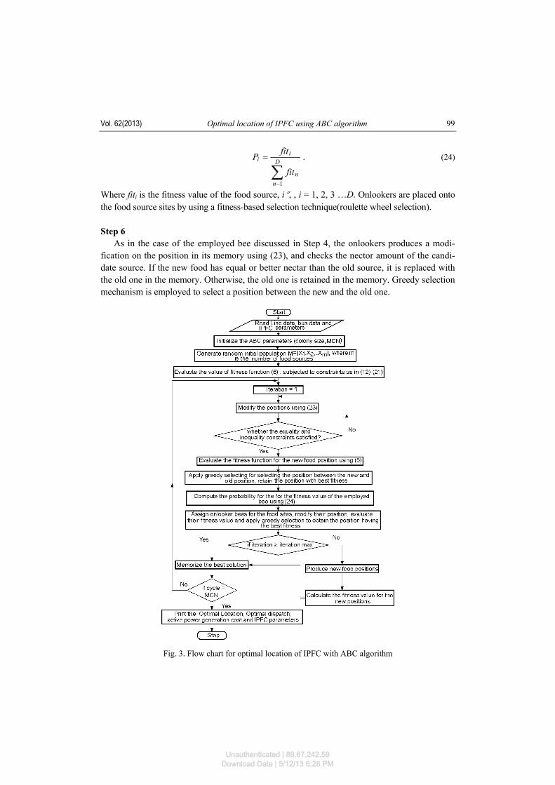
Where fiti is the fitness value of the food source, iO, , i = 1, 2, 3 …D. Onlookers are placed onto the food source sites by using a fitness-based selection technique(roulette wheel selection). Step 6 As in the case of the employed bee discussed in Step 4, the onlookers produces a modi-fication on the position in its memory using (23), and checks the nector amount of the candi-date source. If the new food has equal or better nectar than the old source, it is replaced with the old one in the memory. Otherwise, the old one is retained in the memory. Greedy selection mechanism is employed to select a position between the new and the old one.

Fig. 3. Flow chart for optimal location of IPFC with ABC algorithm



Step7 If the solution for a food source is not improved after a number of trials, the food source is abandoned and the scout bee discovers a new food source with Xi. Memorize the best solution achieved so far and increment the cycle count. Step 8 The process is stopped when the termination criteria is satisfied (MCN). The best fitness and the corresponding food position is memorized at the end of the termination criteria. The cost of IPFC, generation dispatch and the IPFC parameters are computed. The flow chart for the proposed methodology is show in Figure 3.

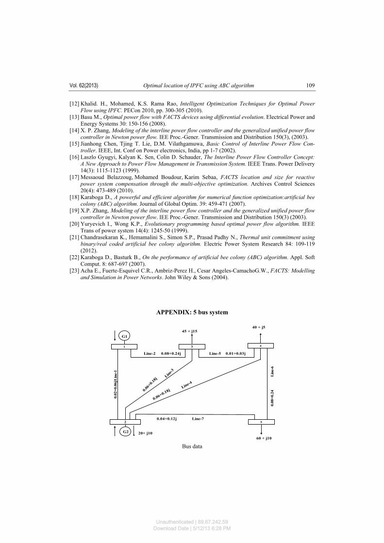
5. Results and discussions The proposed methodology is tested in 5 bus test system [23, Appendix A], IEEE 30 and IEEE 118 bus systems. The parameter settings for ABC are based on trial and error method, and the parameters for various test systems are given in appropriate sections. The minimum and maximum amplitude of converter voltages are chosen as 0.001 p.u and 0.3 p.u. The minimum and maximum phase angle of the two converters are taken as -180o and 180o re-spectively. The effectiveness of IPFC to improve power flow is also discussed in all cases. The cost of IPFC is calculated in all the cases using (11), which depends on the reactive power flow in the line. The optimal location is also carried out using conventional LR method, which is then compared with the non conventional proposed method. The complexity in deriving the Jacobian matrix is eliminated by the proposed methodology. This is executed in MATLAB 7.5 version software with 3 GB RAM. 5.1. Case 1: 5 bus system The IPFC is placed in various locations in 5 bus test system and its effectiveness to im-prove the power flow is given in Table 1. The 5 bus test system is modified to incorporate IPFC in it by adding two dummy lines. The total load of the system is 165 MW. The colony size for ABC is selected as 20 and the termination criteria (MCN) is taken as 100. The para-meters for IPFC and ABC are chosen as given in Section 5. The IPFC is placed in all possible locations and the results (active power dispatch, bus voltages, losses, real power flow, real power generation cost, IPFC installation cost and IPFC parameters) for two lines including the optimal location is summarized in Table 1. IPFC improves the power flow through the lines by injecting real and reactive power of proper magnitude. From Table 1, it is clear that the optimal location is line 4-2-3 in which the active power generation cost and IPFC installation costs are minimum. When IPFC is placed in location 4-2-3, there is an improvement of 12.20% real power flow in line 2-3 with ABC compared to 8.16% with LR method. The real power flow in line 4-2 improved by 4.84% with ABC and 3.02% with LR method with the incorporation of IPFC in line 4-2-3. The real power loss in line 4-2 is reduced by 15.20% with LR and 51.47% with ABC, respectively. The active



power generation cost in this case is 735.4 $/hr with ABC and 757.06 $/hr with LR method. The voltage of buses is within the limit for both the methods, but it is much closer to unity with ABC algorithm.

Table 1. Optimal power flow results and IPFC installation cost of 5 bus system

Line 4-2-3 Line 5- 2-4 IPFC Location /parameters

Lag ABC Lag ABC P1(MW) 82.53 82.13 86.07 84.22 P2(MW) 87.65 85.83 84.2 83.77 Voltage V1 (p.u) 1.06 1.06 1.06 1.06 V2 (p.u) 0.996 1.003 0.990 1.05 V3 (p.u) 0.984 0.996 0.983 0.996 V4 (p.u) 0.979 0.983 0.971 0.9738 V5 (p.u) 0.995 0.997 0.979 1.00 Real power loss (MW) 5.19 2.97 5.25 3.00 Real power flow before placing IPFC – Line – 1 (MW) 27.5 27.5 24 24

Real power flow after placing IPFC – Line – 1 (MW) 28.33 28.83 25.68 26.25

Real power flow before placing IPFC – Line – 2 (MW) 24 24 27.5 27.5

Real power flow after placing IPFC – Line – 2 (MW) 25.96 26.93 27.98 28.42

Real power generation Cost($/hr) 757.067 735.4 757.28 743.5 IPFC installation cost (M $) 0.1509 0.1442 0.1925 0.1899 Vse1 ( p.u) 0.025 0.0246 0.001 0.0125 Vse2( p.u) 0.036 0.0131 0.024 0.0369 θse1( Degree) – 69.14 – 36.63 – 180 – 178.25 θse2( Degree) – 130.92 180 – 80.39 – 82.36

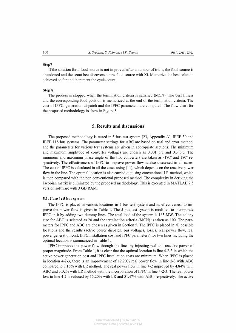
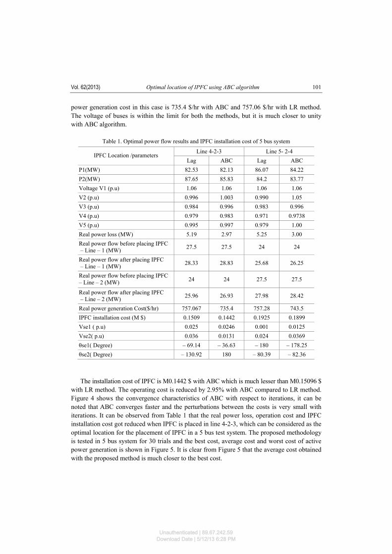
The installation cost of IPFC is M0.1442 $ with ABC which is much lesser than M0.15096 $ with LR method. The operating cost is reduced by 2.95% with ABC compared to LR method. Figure 4 shows the convergence characteristics of ABC with respect to iterations, it can be noted that ABC converges faster and the perturbations between the costs is very small with iterations. It can be observed from Table 1 that the real power loss, operation cost and IPFC installation cost got reduced when IPFC is placed in line 4-2-3, which can be considered as the optimal location for the placement of IPFC in a 5 bus test system. The proposed methodology is tested in 5 bus system for 30 trials and the best cost, average cost and worst cost of active power generation is shown in Figure 5. It is clear from Figure 5 that the average cost obtained with the proposed method is much closer to the best cost.



Fig. 4. Convergence plot for 5 bus system with ABC

Fig. 5. Generation cost for 30 trials in 5 bus system with ABC

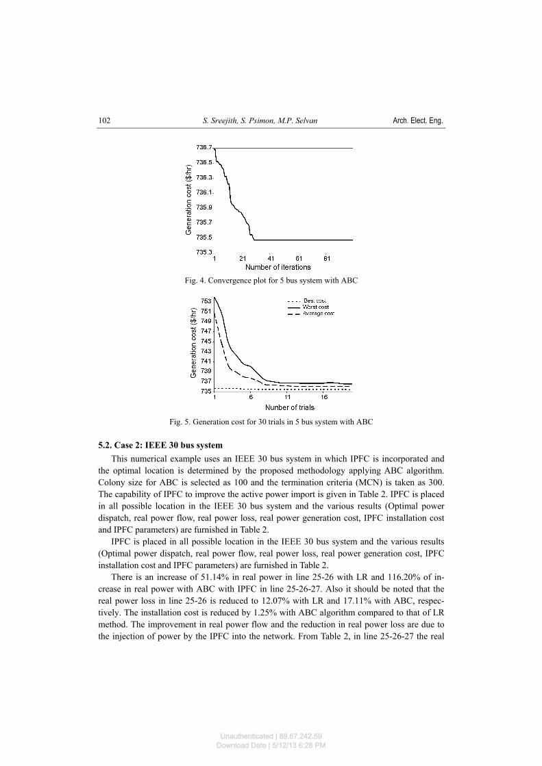
5.2. Case 2: IEEE 30 bus system This numerical example uses an IEEE 30 bus system in which IPFC is incorporated and the optimal location is determined by the proposed methodology applying ABC algorithm. Colony size for ABC is selected as 100 and the termination criteria (MCN) is taken as 300. The capability of IPFC to improve the active power import is given in Table 2. IPFC is placed in all possible location in the IEEE 30 bus system and the various results (Optimal power dispatch, real power flow, real power loss, real power generation cost, IPFC installation cost and IPFC parameters) are furnished in Table 2. IPFC is placed in all possible location in the IEEE 30 bus system and the various results (Optimal power dispatch, real power flow, real power loss, real power generation cost, IPFC installation cost and IPFC parameters) are furnished in Table 2. There is an increase of 51.14% in real power in line 25-26 with LR and 116.20% of in-crease in real power with ABC with IPFC in line 25-26-27. Also it should be noted that the real power loss in line 25-26 is reduced to 12.07% with LR and 17.11% with ABC, respec-tively. The installation cost is reduced by 1.25% with ABC algorithm compared to that of LR method. The improvement in real power flow and the reduction in real power loss are due to the injection of power by the IPFC into the network. From Table 2, in line 25-26-27 the real



power flow is improved to a greater extent. The real power generation cost is 599.45 $/hr with ABC which is lesser than 600.32 $/hr obtained with LR method. The real power loss is 10.03 MW with ABC and 10.64 MW with LR method, which shows the capability of ABC algorithm in reducing real power loss.

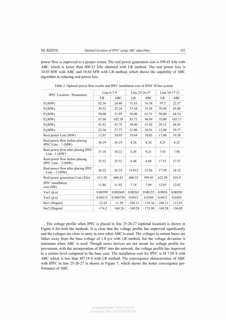
Table 2. Optimal power flow results and IPFC installation cost of IEEE 30 bus system

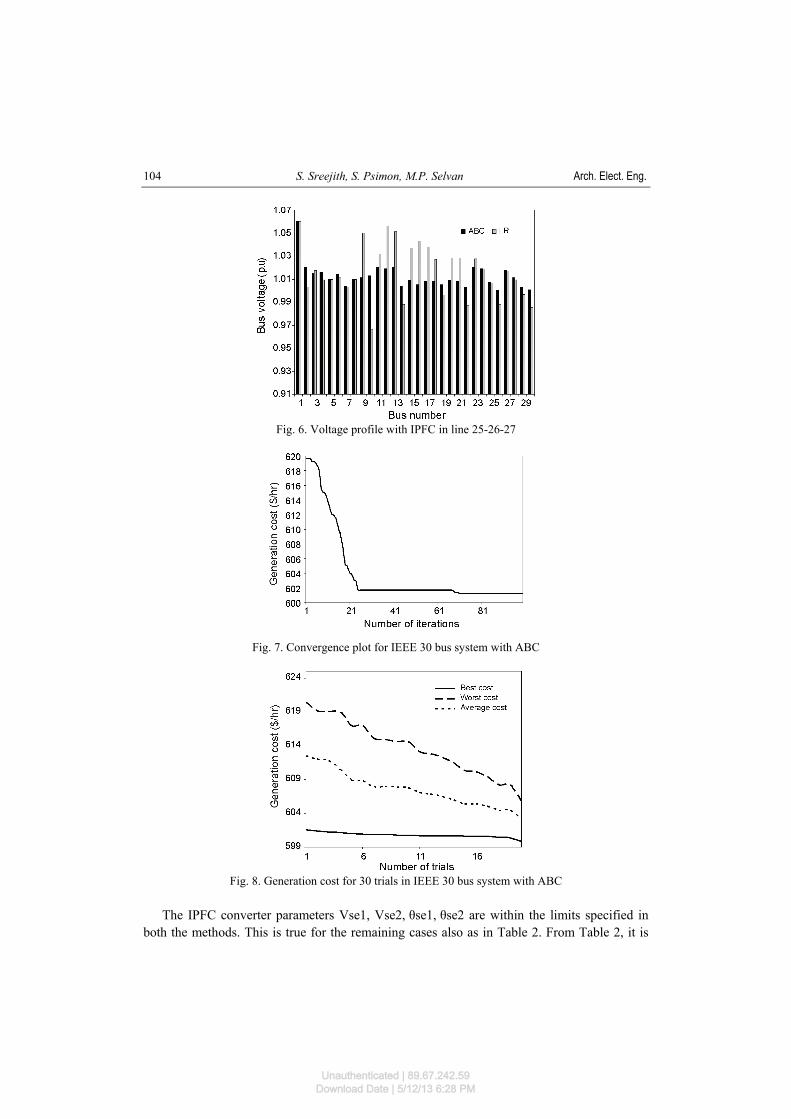
The voltage profile when IPFC is placed in line 25-26-27 (optimal location) is shown in Figure 6 for both the methods. It is clear that the voltage profile has improved significantly and the voltages are close to unity in case when ABC is used. The voltages in certain buses are father away from the base voltage of 1.0 p.u with LR method, but the voltage deviation is minimum when ABC is used. Though series devices are not meant for voltage profile im-provement, with the incorporation of IPFC into the network, the voltage profile has improved to a certain level compared to the base case. The installation cost for IPFC is M 7.09 $ with ABC which is less than M7.18 $ with LR method. The convergence characteristics of ABC with IPFC in line 25-26-27 is shown in Figure 7, which shows the better convergence per-formance of ABC.

Line 6-7-9 Line 25-26-27 Line 10-17-21 IPFC Location / Parameters

LR ABC LR ABC LR ABC P1(MW) 62.16 24.48 71.63 16.38 97.3 22.37 P2(MW) 39.32 32.24 37.64 31.38 70.98 05.00 P3(MW) 50.00 51.95 50.00 61.31 50.00 64.54 P4(MW) 67.66 102.10 83.73 96.89 35.00 103.17 P5(MW) 41.82 45.75 30.00 51.42 29.12 68.43 P6(MW) 22.36 37.77 21.00 36.01 12.00 29.77 Real power Loss (MW) 11.07 10.93 10.64 10.03 11.00 10.38 Real power flow before placing IPFC Line – 1 (MW) 36.19 36.19 4.26 4.26 4.25 4.25

Real power flow after placing IPFC – Line –1 (MW) 37.18 38.22 6.45 9.21 7.93 7.98

Real power flow before placing IPFC Line – 2 (MW) 25.32 25.32 6.68 6.68 17.51 17.51

Real power flow after placing IPFC – Line – 2 (MW) 26.22 26.19 19.912 21.06 17.99 18.12

Real power generation Cost ($/hr) 611.58 600.45 600.32 599.45 622.58 618.9 IPFC installation cost (M$) 11.86 11.92 7.18 7.09 12.05 12.02

Vse1 (p.u) 0.00399 0.002645 0.00263 0.00125 0.0026 0.00289 Vse2 (p.u) 0.04212 0.504728 0.0412 0.0369 0.0412 0.0458 θse1 (Degree) !12.63 !11.39 !106.11 !110.36 !106.11 !113.65 θse2 (Degree) !174.2 !168.26 !169.28 !173.98 !169.28 !156.85



Fig. 6. Voltage profile with IPFC in line 25-26-27

Fig. 7. Convergence plot for IEEE 30 bus system with ABC

Fig. 8. Generation cost for 30 trials in IEEE 30 bus system with ABC

The IPFC converter parameters Vse1, Vse2, θse1, θse2 are within the limits specified in both the methods. This is true for the remaining cases also as in Table 2. From Table 2, it is



clear that the IPFC installation cost, active power generation cost and power loss has reduced to a considerable amount when IPFC is placed in line 25-26-27 (optimal location). The proposed methodology is tested for 30 trials in IEEE 30 bus system and the best cost, average cost and worst cost of active power generation is shown in Figure 8. It is clear from Figure 8 that the average cost obtained with the proposed method is closer to the best cost. 5.3. Case 3: IEEE 118 bus system Here the optimal location of IPFC in 118 bus test system is carried out using ABC algo-rithm. The line and bus data are modified to incorporate IPFC in it. The colony size for ABC is selected as 50 and the termination criteria (MCN) is taken as 200. The IPFC is placed in all the possible positions in the test system and the results for 3 cases are illustrated in Table 3.

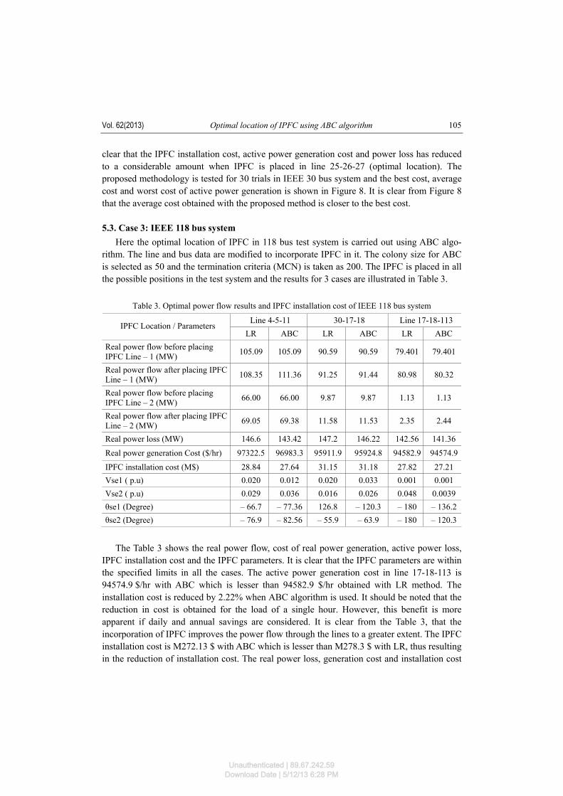
Table 3. Optimal power flow results and IPFC installation cost of IEEE 118 bus system

Line 4-5-11 30-17-18 Line 17-18-113 IPFC Location / Parameters

LR ABC LR ABC LR ABC Real power flow before placing IPFC Line – 1 (MW) 105.09 105.09 90.59 90.59 79.401 79.401

Real power flow after placing IPFC Line – 1 (MW) 108.35 111.36 91.25 91.44 80.98 80.32

Real power flow before placing IPFC Line – 2 (MW) 66.00 66.00 9.87 9.87 1.13 1.13

Real power flow after placing IPFC Line – 2 (MW) 69.05 69.38 11.58 11.53 2.35 2.44

Real power loss (MW) 146.6 143.42 147.2 146.22 142.56 141.36

Real power generation Cost ($/hr) 97322.5 96983.3 95911.9 95924.8 94582.9 94574.9

IPFC installation cost (M$) 28.84 27.64 31.15 31.18 27.82 27.21 Vse1 ( p.u) 0.020 0.012 0.020 0.033 0.001 0.001 Vse2 ( p.u) 0.029 0.036 0.016 0.026 0.048 0.0039 θse1 (Degree) – 66.7 – 77.36 126.8 – 120.3 – 180 – 136.2 θse2 (Degree) – 76.9 – 82.56 – 55.9 – 63.9 – 180 – 120.3

The Table 3 shows the real power flow, cost of real power generation, active power loss, IPFC installation cost and the IPFC parameters. It is clear that the IPFC parameters are within the specified limits in all the cases. The active power generation cost in line 17-18-113 is 94574.9 $/hr with ABC which is lesser than 94582.9 $/hr obtained with LR method. The installation cost is reduced by 2.22% when ABC algorithm is used. It should be noted that the reduction in cost is obtained for the load of a single hour. However, this benefit is more apparent if daily and annual savings are considered. It is clear from the Table 3, that the incorporation of IPFC improves the power flow through the lines to a greater extent. The IPFC installation cost is M272.13 $ with ABC which is lesser than M278.3 $ with LR, thus resulting in the reduction of installation cost. The real power loss, generation cost and installation cost



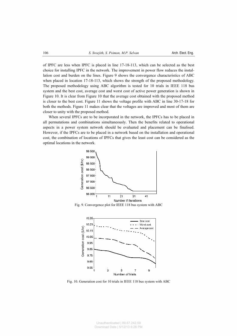
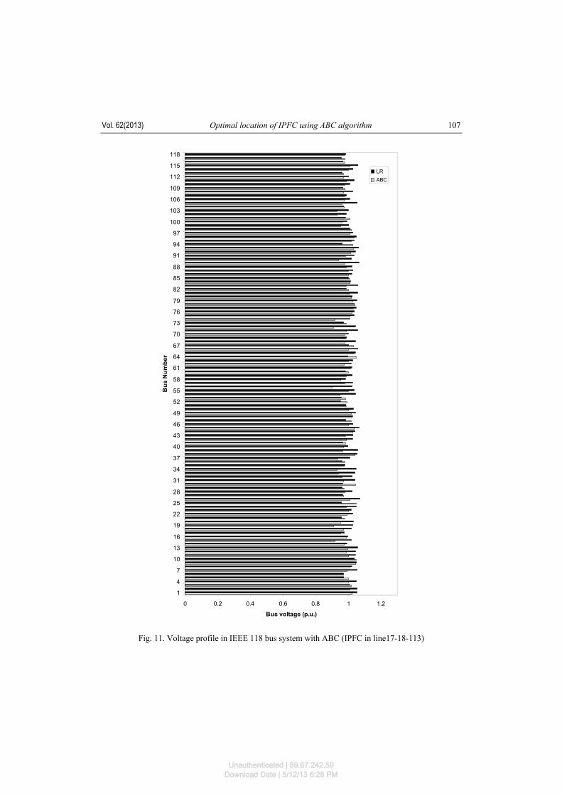
of IPFC are less when IPFC is placed in line 17-18-113, which can be selected as the best choice for installing IPFC in the network. The improvement in power flow reduces the instal-lation cost and burden on the lines. Figure 9 shows the convergence characteristics of ABC when placed in location 17-18-113, which shows the strength of the proposed methodology. The proposed methodology using ABC algorithm is tested for 10 trials in IEEE 118 bus system and the best cost, average cost and worst cost of active power generation is shown in Figure 10. It is clear from Figure 10 that the average cost obtained with the proposed method is closer to the best cost. Figure 11 shows the voltage profile with ABC in line 30-17-18 for both the methods. Figure 11 makes clear that the voltages are improved and most of them are closer to unity with the proposed method. When several IPFCs are to be incorporated in the network, the IPFCs has to be placed in all permutations and combinations simultaneously. Then the benefits related to operational aspects in a power system network should be evaluated and placement can be finalised. However, if the IPFCs are to be placed in a network based on the installation and operational cost, the combination of locations of IPFCs that gives the least cost can be considered as the optimal locations in the network.

Fig. 9. Convergence plot for IEEE 118 bus system with ABC

Fig. 10. Generation cost for 10 trials in IEEE 118 bus system with ABC



0 0.2 0.4 0.6 0.8 1 1.2

1

4

7

10

13

16

19

22

25

28

31

34

37

40

43

46

49

52

55

58

61

64

67

70

73

76

79

82

85

88

91

94

97

100

103

106

109

112

115

118B

us N

umbe

r

Bus voltage (p.u.)

LRABC

Fig. 11. Voltage profile in IEEE 118 bus system with ABC (IPFC in line17-18-113)



4. Conclusion The optimal location of IPFC in a power system network is identified by using both the conventional (Lagrangian Relaxation) and non conventional (ABC) method by considering the minimization in installation cost, active power generation cost, improvement in power flow and reduction in real power losses in the power system network. The cost function for IPFC is derived from the existing cost function of UPFC. The proposed method and the LR method are validated with standard benchmark systems like 5 bus, IEEE 30 bus and IEEE 118 bus test systems. Considerable reduction in generation cost, real power loss, improvement in power flow and voltage profile improvement are obtained with the proposed methodology. The optimal location for the placement of IPFC is clearly demonstrated for all test systems. Economic load dispatch is carried out for all the test systems which results in significant annual savings in operational cost of the system. The computational complexity and the rate of convergence for both the methods are addressed. The results afford evidence that the proposed ABC methodology is found to be effective than conventional LR method in obtaining both quality solution and good convergence rate. Also other FACTS devices such as SVC, TCSC, SSSC, STATCOM and UPFC can be investigated and the performance evaluation can be carried out by the proposed method. The proposed method can be extended to practical and large power system networks. References [1] Hingorani N.G., Gyugyi L., Understanding FACTS: Concepts and Technology of Flexible AC Trans-

mission Systems. Wiley-IEEE Press (1999). [2] Nogal T.Ł., Machowski J., WAMS – based control of series FACTS devices installed in tie-lines of

interconnected power system. Archives of Electrical Engineering: 59(3-4): 121-140 (2010). [3] Saravanan M., Mary Raja Slochanal S., Venkatesh P., Prince Stephen Abraham J., Application of

particle swarm optimization technique for optimal location of FACTS devices considering cost of installation and system loadability. Electric Power Systems Research 77: 276-283 (2007).

[4] Lie T.T., Deng W., Optimal Flexible AC Transmission Systems (FACTS) devices allocation. Electri-cal Power & Energy Systems 9:129-134 (1997).

[5] Cai L.J., Erlich I., Optimal choice and allocation of FACTS devices using genetic algorithms. Proce-edings on Twelfth Intelligent Systems Application to Power Systems Conference, pp. 1-6 (2003).

[6] Sarvi M., Sedighizadeh M., Qarebaghi J., Optimal Location and Parameters Setting of UPFC Based on Particle Swarm Optimization for Increasing Loadability. International Review of Electrical En-gineering 5(5): 2234-2240 (2010).

[7] Bekri O.L., Fellah M.K., Benkhoris M.F., Miloudi A., Voltage Stability Enhancement by Optimal SVC and TCSC Location Via CP Flow Analysis. International Review of Electrical Engineering 5(5): 2263-2270 (2010).

[8] Zuwei Yu, Lusan D., Optimal placement of FACTs devices in deregulated systems considering line losses. Electrical Power and Energy Systems 26: 813-819 (2004).

[9] Umapom Kwannetr, Uthen Leeton, Thanatchai Kulworawanichpong, Optimal Power Flow Using Artificial Bees Algorithm. 2010 International Conference on Advances in Energy Engineering, pp: 215-218 (2010).

[10] Karaboga D., Basturk B., Artificial Bee Colony (ABC) Optimization Algorithm for Solving Constrai-ned Optimization Problems. Springer-Verlag, pp. 789-798 (2007).

[11] Teerathana S., Yokoyama A., An optimal power flow control method of power system using inter-line power flow controller (IPFC). TENCON 2004. IEEE Region 10 Conference 3: 343-346 (2004).



[12] Khalid. H., Mohamed, K.S. Rama Rao, Intelligent Optimization Techniques for Optimal Power Flow using IPFC. PECon 2010, pp. 300-305 (2010).

[13] Basu M., Optimal power flow with FACTS devices using differential evolution. Electrical Power and Energy Systems 30: 150-156 (2008).

[14] X. P. Zhang, Modeling of the interline power flow controller and the generalized unified power flow controller in Newton power flow. IEE Proc.-Gener. Transmission and Distribution 150(3), (2003).

[15] Jianhong Chen, Tjing T. Lie, D.M. Vilathgamuwa, Basic Control of Interline Power Flow Con-troller. IEEE, Int. Conf on Power electronics, India, pp 1-7 (2002).

[16] Laszlo Gyugyi, Kalyan K. Sen, Colin D. Schauder, The Interline Power Flow Controller Concept: A New Approach to Power Flow Management in Transmission System. IEEE Trans. Power Delivery 14(3): 1115-1123 (1999).

[17] Messaoud Belazzoug, Mohamed Boudour, Karim Sebaa, FACTS location and size for reactive power system compensation through the multi-objective optimization. Archives Control Sciences 20(4): 473-489 (2010).

[18] Karaboga D., A powerful and efficient algorithm for numerical function optimization:artificial bee colony (ABC) algorithm. Journal of Global Optim. 39: 459-471 (2007).

[19] X.P. Zhang, Modeling of the interline power flow controller and the generalized unified power flow controller in Newton power flow. IEE Proc.-Gener. Transmission and Distribution 150(3) (2003).

[20] Yuryevich I., Wong K.P., Evolutionary programming based optimal power flow algorithm. IEEE Trans of power system 14(4): 1245-50 (1999).

[21] Chandrasekaran K., Hemamalini S., Simon S.P., Prasad Padhy N., Thermal unit commitment using binary/real coded artificial bee colony algorithm. Electric Power System Research 84: 109-119 (2012).

[22] Karaboga D., Basturk B., On the performance of artificial bee colony (ABC) algorithm. Appl. Soft Comput. 8: 687-697 (2007).

[23] Acha E., Fuerte-Esquivel C.R., Ambriz-Perez H., Cesar Angeles-CamachoG.W., FACTS: Modelling and Simulation in Power Networks. John Wiley & Sons (2004).

APPENDIX: 5 bus system

1 3 4

2 5

G1

G2 20+ j1060 + j10

40 + j545 + j15

Line

-1

Line-2

Line-3

Line-4

Line-5

Line-7

Line

-6

0.08+0.24j 0.01+0.03j

0.02

+0.0

6j

0.06+

0.18j

0.06+0.18j

0.04+0.12j

0.08

+0.2

4

Bus data



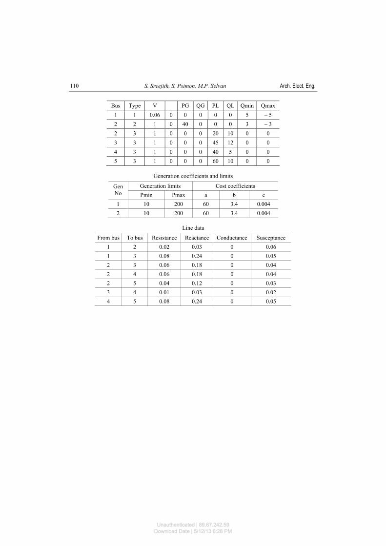
Bus Type V PG QG PL QL Qmin Qmax 1 1 0.06 0 0 0 0 0 5 – 5 2 2 1 0 40 0 0 0 3 – 3 2 3 1 0 0 0 20 10 0 0 3 3 1 0 0 0 45 12 0 0 4 3 1 0 0 0 40 5 0 0 5 3 1 0 0 0 60 10 0 0

Generation coefficients and limits

Generation limits Cost coefficients Gen No Pmin Pmax a b c 1 10 200 60 3.4 0.004 2 10 200 60 3.4 0.004

Line data

From bus To bus Resistance Reactance Conductance Susceptance 1 2 0.02 0.03 0 0.06 1 3 0.08 0.24 0 0.05 2 3 0.06 0.18 0 0.04 2 4 0.06 0.18 0 0.04 2 5 0.04 0.12 0 0.03 3 4 0.01 0.03 0 0.02 4 5 0.08 0.24 0 0.05


optimal location of interline power flow controller in a...

Documents