Optimal Multi-scale Patterns in Time Series Streams

Spiros PapadimitriouIBM T.J. Watson Research Center

Hawthorne, NY, USA

spapadim@us.ibm.com

Philip S. YuIBM T.J. Watson Research Center

Hawthorne, NY, USA

psyu@us.ibm.com

ABSTRACTWe introduce a method to discover optimal local patterns,which concisely describe the main trends in a time series.Our approach examines the time series at multiple timescales (i.e., window sizes) and efficiently discovers the keypatterns in each. We also introduce a criterion to selectthe best window sizes, which most concisely capture thekey oscillatory as well as aperiodic trends. Our key insightlies in learning an optimal orthonormal transform from thedata itself, as opposed to using a predetermined basis orapproximating function (such as piecewise constant, short-window Fourier or wavelets), which essentially restricts usto a particular family of trends. Our method lifts that lim-itation, while lending itself to fast, incremental estimationin a streaming setting. Experimental evaluation shows thatour method can capture meaningful patterns in a variety ofsettings. Our streaming approach requires order of magni-tude less time and space, while still producing concise andinformative patterns.

1. INTRODUCTIONData streams have recently received much attention in sev-eral communities (e.g., theory, databases, networks, datamining) because of several important applications (e.g., net-work traffic analysis, moving object tracking, financial dataanalysis, sensor monitoring, environmental monitoring, sci-entific data processing).

Many recent efforts concentrate on summarization and pat-tern discovery in time series data streams [5, 23, 24, 33, 4,26, 6]. Typical approaches for pattern discovery and summa-rization of time series rely on fixed transforms, with a pre-determined set of bases [24, 33] or approximating functions[5, 23, 4]. For example, the short-window Fourier transformuses translated sine waves of fixed length and has been suc-cessful in speech processing [28]. Wavelets use translatedand dilated sine-like waves and have been successfully ap-plied to more bursty data, such as images and video streams

Permission to make digital or hard copies of all or part of this work forpersonal or classroom use is granted without fee provided that copies arenot made or distributed for profit or commercial advantage and that copiesbear this notice and the full citation on the first page. To copy otherwise, torepublish, to post on servers or to redistribute to lists, requires prior specificpermission and/or a fee.SIGMOD 2006, June 27–29, 2006, Chicago, Illinois, USA.Copyright 2006 ACM 1-59593-256-9/06/0006 ...$5.00.

[32]. Furthermore, selecting a wavelet basis to match thetime series’ characteristics is a non-trivial problem [32, 27,30]. Thus, even though these approaches have been usefulfor pattern discovery in a number of application domains,there is no single method that is best for arbitrary timeseries.

We propose to address this problem by learning the appro-priate approximating functions directly from the data, in-stead of using a fixed set of such functions. Our methodestimates the “eigenfunctions” of the time series in finite-length time windows. Similar ideas have been used in otherareas (e.g., image denoising or motion capture). However,our approach examines the data at multiple time scales and,to the best of our knowledge, the problem of estimating theseeigenfunctions incrementally has not been studied before.

1 2 3 4 5

x 104

0

500

1000

1500

2000

Automobile

Time

Figure 1: Automobile traffic data (aggregate countsfrom a west coast interstate).

ExampleWe will illustrate the main intuition and motivation with areal example. Figure 1 shows automobile traffic counts in alarge, west coast interstate. The data exhibit a clear dailyperiodicity. Also, in each day there is another distinct pat-tern of morning and afternoon rush hours. However, thesepeaks have distinctly different shapes: the morning one ismore spread out, the evening one more concentrated andslightly sharper. What we would ideally like to discover is:

1. The main trend in the data repeats at a window (“pe-riod”) of approximately 4000 timestamps.

2. A succinct “description” of that main trend that cap-tures most of the recurrent information.

Figure 2a shows the output of our pattern discovery ap-proach, which indeed suggests that the “best” window is

1000 2000 3000 4000−0.06

−0.04

−0.02

0

0.02

0.04

0.06

Time (1..4000)

First pattern (basis)

1000 2000 3000 4000−0.06

−0.04

−0.02

0

0.02

0.04

0.06

Time (1..4000)

Second pattern (basis)

1000 2000 3000−0.04

−0.02

0

0.02

0.04

Time (1..3645)

First pattern (hierarchical, streaming)

1000 2000 3000−0.04

−0.02

0

0.02

0.04

Time (1..3645)

Second pattern (hierarchical, streaming)

0 2000 4000

−0.02

−0.01

0

0.01

0.02

First basis (DCT)

Time (1..4000)0 2000 4000

−0.02

−0.01

0

0.01

0.02

Second basis (DCT)

Time (1..4000)0 2000 4000

−0.02

−0.01

0

0.01

0.02

Third basis (DCT)

Time (1..4000)

(a) Representative patterns (b) Representative patterns (c) Fixed bases (DCT) with highest coefficients,(batch, non-hierarchical), 5.4% error. (streaming, hierarchical). 7.7% error (8.4% with two coefficients).

Figure 2: Automobile traffic, best selected window (about 1 day) and corresponding representative patterns.

4000 timestamps. Furthermore, the first pattern capturesthe average and the second pattern correctly captures thetwo peaks and also their approximate shape (the first onewide and the second narrower). For comparison, in Fig-ure 2b we show the output of our fast, streaming computa-tion scheme. In order to reduce the storage and computationrequirements, our fast scheme tries to filter out some of the“noise” earlier, while retaining as many of the regularities aspossible. However, which information should be discardedand which should be retained is once again decided basedon the data itself. Thus, even though we unavoidably dis-card some information, Figure 2b still correctly captures themain trends (average level, peaks and their shape).

For comparison, Figure 2c shows the best “local patterns”we would obtain using fixed bases. For illustration, we chosethe Discrete Cosine Transform (DCT) on the first window of4000 points. First, most fixed-basis schemes cannot be easilyused to capture information at arbitrary time scales (withthe exception of wavelets). More importantly, any fixed-basis scheme (e.g., wavelets, Fourier, etc) would producesimilar results which are heavily biased towards the shapeof the a priori chosen bases or approximating functions.

ContributionsWe introduce a method that can learn the key trends in atime series. Our main contributions are:

• We introduce the notion of optimal local patterns intime series, which concisely describe the main trends,both oscillatory as well as aperiodic, within a fixedwindow.

• We show how to extract trends at multiple time scales(i.e., window sizes).

• We propose a criterion which allows us to choose thebest window sizes from the data.

• We introduce an approach to perform all of the aboveincrementally, in a streaming setting.

We evaluate our approach on real data and show that it dis-covers meaningful patterns. The streaming approach achieves1-4 orders of magnitude improvement in time and space re-quirements.

In the rest of this paper we answer the following questions:

1. Given a window, how do we find locally optimal pat-terns?

2. How can we compare the information captured by pat-terns at different window sizes?

3. How can we efficiently compute patterns at several dif-ferent window sizes and quickly zero-in on the “best”window?

4. How can we do all of the above incrementally, in astreaming setting?

After reviewing some of the background in Section 2 andintroducing necessary definitions and notation in Section 3,we answer the first two questions in Section 4. We answerthe third question in Section 5, which introduces an efficientscheme for pattern discovery at multiple scales. Section 6answers the fourth question. Section 7 demonstrates theeffectiveness of our approach on real data. Finally, Section 8discusses related work and Section 9 concludes.

2. BACKGROUNDIn this section we describe some of the basic background.For more details, the reader can see, e.g., [29]. We use bold-face lowercase letters for column vectors, v ≡ [v1 v2 · · · vn]T ∈R

n, and boldface capital letters for matrices, A ∈ Rm×n.

Finally, we adopt the notation aj for the columns of A ≡[a1 a2 · · · a3] and a(i) for the rows of A ≡ [a(1) a(2) · · · a(m)]

T .Note that a(i) are also column vectors, not row vectors—we always represent vectors as column vectors. For ma-trix/vector elements we use either subscripts, aij , or brack-ets, a[i, j].

The rows of A are points in an (at most) n-dimensionalspace, a(i) ∈ R

n, which is the row space of A. The actualdimension of the row space is the rank r of A. It turnsout that we can always find a “special” orthonormal basisfor the row space, which defines a new coordinate system(see Figure 3). If vj is a unit-length vector defining one ofthe axes in the row space then, for each row a(i), it’s j-th

coordinate in the new axes is the dot product aT(i)vj =: pij

so that, if V := [v1 · · · vr] and we define P := AV, theneach row of P is the same point as the corresponding row ofA but with respect to the new coordinate system. Thereforelengths and distances are preserved, i.e. ‖a(i)‖ = ‖p(i)‖ and‖a(i) − a(j)‖ = ‖p(i) − p(j)‖, for all 1 ≤ i, j ≤ m.

However, the new coordinate system is “special” in the fol-lowing sense. Say we keep only the first k columns of P (let’s

call this matrix P) thus effectively projecting each point intoa space with lower dimension k. Also, rows of the matrix

A := PVT (1)

pv2

1v

a(i)

ai1

ai2 a(i)

i2p

i1

Figure 3: Illustration of SVD (for dimension n = 2),with respect to row space. Each point correspondsto a row of the matrix A and vj, j = 1, 2 are theleft singular vectors of A. The square is the one-dimensional approximation of a(i) by projecting itonto the first singular vector.

are the same points translated back into the original co-ordinate system of the row space (the square in Figure 3,

if k = 1), where V consists of the first k columns of V.

Then P maximizes the sum of squares ‖P‖2F =Pm,k

i,j=1 p2ij

or, equivalently, minimizes the sum of squared residual dis-tances (thick dotted line in Figure 3, if k = 1), ‖X− X‖2F =Pm

i=1 ‖x(i) − x(i)‖2.

Therefore, from the point of view of the row space, we canwrite A = PVT . We can do the same for the columnspace of A and get A = UQT , where U is also column-orthonormal, like V. It turns out that U and V have aspecial significance, which is formally stated as follows:

Theorem 1 (Singular value decomposition). Everymatrix A ∈ R

m×n can be decomposed into

A = UΣVT

where U ∈ Rm×r, V ∈ R

n×r and Σ ∈ Rr×r, with r ≤

min(m, n) the rank of A. The columns vi of V ≡ [v1 · · · vr]are the right singular vectors of A and they form an or-thonormal basis its row space. Similarly, the columns ui ofU ≡ [u1 · · · ur] are the left singular vectors and form a ba-sis of the column space of A. Finally Σ ≡ diag[σ1 · · · σr] isa diagonal matrix with positive values σi, called the singularvalues of A.

From the above, the matrix of projections P is P = UΣ.Next, we can formally state the properties of a low-dimensionalapproximation using the first k singular values (and corre-sponding singular vectors) of A:

Theorem 2 (Low-rank approximation). If we keeponly the singular vectors corresponding to the k highest sin-gular values (k < r), i.e. if U := [u1 u2 · · · uk], V :=

[v1 v2 · · · vk] and Σ = diag[σ1 σ2 · · · σk], then A = UΣVT

is the best approximation of A, in the sense that it minimizesthe error

‖A− A‖2F :=Pm,n

i,j=1 |aij − aij |2 =

Pri=k+1 σ2

i . (2)

In Equation (2), note the special significance of the singularvalues for representing the approximation’s squared error.

Symbol Description

y Vector A ∈ Rn (lowercase bold), always col-

umn vectors.A Matrix A ∈ R

m×n (uppercase bold).aj j-th column of matrix Aa(i) i-th row of matrix A, as a column vector.‖y‖ Euclidean norm of vector y.‖A‖F Frobenius norm of matrix A, ‖A‖2F =

Pm,ni,j=1 a2

ij .

X Time series matrix, with each row corre-sponding to a timestamp.

X(w) The delay coordinates matrix correspondingto X, for window w.

V(w) Right singular vectors of X(w).

Σ(w) Singular values of X(w).

U(w) Left singular vectors of X(w).

k Dimension of approximating subspace.

V(w) Same as V(w), Σ(w), U(w) but only with

Σ(w) with k highest singular values and vectors.

U(w)

P(w) Projection of X(w) onto first k right singularvectors, P(w) := U(w)Σ(w) = X(w)V(w).

V(w0,l) Hierarchical singular vectors, values and

Σ(w0,l) projections, for the k highest singular

P(w0,l) values.

V0(w0,l) Hierarchically estimated patterns (bases).

Table 1: Frequently used notation.

Furthermore, since U and V are orthonormal, we havePr

i=1 σ2i = ‖A‖2F and

Pki=1 σ2

i = ‖A‖2F . (3)

3. PRELIMINARIESIn this section we give intuitive definitions of the problemswe are trying to solve. We also introduce some conceptsneeded later.

Ideally, a pattern discovery approach for arbitrary time se-ries (where we have limited or no prior knowledge) shouldsatisfy the following requirements:

1. Data-driven: The approximating functions should bederived directly from the data. A fixed, predeterminedset of bases or approximating functions may (i) misssome information, and (ii) discovers patterns that arebiased towards the “shape” of those functions.

2. Multi-scale: We do not want to restrict examination toa finite, predetermined maximum window size, or wewill miss long range trends that occur at time scaleslonger than the window size.

Many approaches assume a fixed-length, sliding window. Inthe majority of cases, this restriction cannot be triviallylifted. For example, short-window Fourier cannot say any-thing about periods larger than the sliding window length.Wavelets are by nature multi-scale, but they still use a fixedset of bases, which is also often hard to choose [27, 32].

The best way to conceptually summarize the main differ-ence of our approach is the following: typical methods first

project the data onto “all” bases in a given family (e.g.,Fourier, wavelets, etc) and then choose a few coefficientsthat capture the most information. In contrast, among allpossible bases we first choose a few bases that are guaranteedto capture the most information and consequently projectthe data only onto those. However, efficiently determiningthese few bases and incrementally updating them as newpoints arrive is a challenging problem.

With respect to the first of the above requirements (data-driven), let us assume that someone gives us a window size.Then, the problem we want to solve (addressed in Section 4)is the following:

Problem 1 (Fixed-window optimal patterns). Givena time series xt, t = 1, 2, . . . and a window size w, find thepatterns that best summarize the series at this window size.

The patterns are w-dimensional vectors vi ≡ [vi,1, . . . , vi,w]T ∈R

w, chosen so that they capture “most” of the informationin the series (in a way that we will make precise later).

In practice, however, we do not know a priori the right win-dow size. Therefore, with respect to the second requirement(multi-scale), we want to solve the following problem (ad-dressed in Section 5):

Problem 2 (Optimal local patterns). Given a timeseries xt and a set of windows W := {w1, w2, w3, . . .}, find(i) the optimal patterns for each of these, and (ii) the bestwindow w∗ to describe the key patterns in the series.

So how do we go about finding these patterns? An elemen-tary concept we need to introduce is time-delay coordinates.We are given a time series xt, t = 1, 2, . . . with m pointsseen so far. Intuitively, when looking for patterns of lengthw, we divide the series in consecutive, non-overlapping sub-sequences of length w. Thus, if the original series is a m× 1matrix (not necessarily materialized), we substitute it witha m

w× w matrix. Instead of m scalar values we now have a

sequence of m/w vectors with dimension w. It is natural tolook for patterns among these time-delay vectors.

Definition 1 (Delay coordinates). Given a sequencex ≡ [x1, x2, . . . , xt, . . . , xm]T and a delay (or window) w, thedelay coordinates are a ⌈m/w⌉×w matrix with the t′-th row

equal to X(w)

(t′) := [x(t′−1)w+1, x(t′−1)w+2, . . . , xt′w]T .

Of course, neither x nor X(w) need to be fully materializedat any point in time. In practice, we only need to store thelast row of X(w).

Also, note that we choose non-overlapping windows. Wecould also use overlapping windows, in which case X(w)

would have m − w + 1 rows, with row t consisting of val-ues xt, xt+1, . . . , xt+w. In this case, there are some subtledifferences [12], akin to the differences between “standard”wavelets and maximum-overlap or redundant wavelets [27].However, in practice non-overlapping windows are equally

effective for pattern discovery and also lend themselves bet-ter to incremental, streaming estimation using limited re-sources.

More generally, the original time series does not have to bescalar, but can also be vector-valued itself. We still do thesame, only each row of X(w) is now a concatenation of rowsof X (instead of a concatenation of scalar values). More pre-cisely, we construct the general time-delay coordinate matrixas follows:

Procedure 1 Delay (X ∈ Rm×n, w)

m′ ← ⌊m/w⌋ and n′ ← nw

Output is X(w) ∈ Rm′×n′

{not necessarily materialized}for t = 1 to m′ do

Row X(w)(t) ← concatenation of rows

X((t−1)w+1),X((t−1)w+2), · · ·X(tw)

end for

Incremental SVDBatch SVD algorithms are too costly. For an m× n matrixA, even finding only the highest singular value and corre-sponding singular vector needs time O(n2m), where n < m.Aside from computational cost, we also need to incremen-tally update the SVD as new rows are added to A.

SVD update algorithms such as [3, 13] can support bothrow additions as well as deletions. However, besides theright singular vectors vi, both of these approaches need tostore the left singular vectors ui (whose size is proportionalto the time series length in our case).

Algorithm 1 IncrementalSVD (A, k)

for i = 1 to k doInitialize vi to unit vectors, vi ← iiInitialize σ2

i to small positive value, σ2i ← ǫ

end forfor all new rows a(t+1) do

Initialize a← a(t+1)

for i = 1 to k doyi ← vT

i a {projection onto vi}σ2

i ← σ2i + y2

i {energy ∝ singular value}ei ← a− yivi {error, ei ⊥ vi}vi ← vi + 1

σ2i

yiei {update singular vector estimate}

a← a− yivi {repeat with remainder of a(t+1)}end forp(t+1) ← VT a(t+1) {final low-dim. projection of a(t+1)}

end for

We chose an SVD update algorithm (shown above, for givennumber k of singular values and vectors) that has been suc-cessfully applied in streams [25, 34]. Its accuracy is stillvery good, while it does not need to store the left singu-lar vectors. Since our goal is to find patterns at multiplescales without an upper bound on the window size, this is amore suitable choice. Furthermore, if we need to place moreemphasis on recent trends, it is rather straightforward toincorporate an exponential forgetting scheme, which workswell in practice [25]. For each new row, the algorithm up-dates k · n numbers, so total space requirements are O(nk)and the time per update is also O(nk). Finally, the incre-mental update algorithms need only the observed values and

x timedelayed

coordinates

v1(w) and projections

local patterns

X(w)

v2(w)

proj. proj. proj. proj.

local bases(patterns)

Figure 4: Illustration of local patterns for a fixedwindow (here, w = 4).

can therefore easily handle missing values by imputing thembased on current estimates of the singular vectors [25].

4. LOCALLY OPTIMAL PATTERNSWe now have all the pieces in place to answer the first ques-tion: for a given window w, how do we find the locallyoptimal patterns? Figure 4 illustrates the main idea. Start-ing with the original time series x, we transfer to time-delaycoordinates X(w). The local patterns are the right singularvectors of X(w), which are optimal in the sense that theyminimize the total squared approximation error of the rows

X(w)

(i) . The detailed algorithm is shown below.

Algorithm 2 LocalPattern (x ∈ Rm, w, k = 3)

Use delay coord. X(w) ← Delay(x, w)

Compute SVD of X(w) = U(w)Σ(w)V(w)

Local patterns are v(w)1 , . . . ,v

(w)k

Power is π(w) ←Pw

i=k+1 σ2i /w =

`Pm

t=1 x2t −

Pki=1 σ2

i

´

/w

P(w) ← U(w)Σ(w) {low-dim. proj. onto local patterns}

return V(w), P(w), Σ(w) and π(w)

For now, the projections P(w) onto the local patterns v(i)

are not needed, but we will use them later, in Section 5.Also, note that LocalPattern can be applied in general ton-dimensional vector-valued series. The pseudocode is thesame, since Delay can also operate on matrices X ∈ R

m×n.The reason for this will also become clear in Section 5, butfor now it suffices to observe that the first argument of Lo-calPattern may be a matrix, with one row x(t) ∈ R

n pertimestamp t = 1, 2, . . . , m.

When computing the SVD, we really need only the highestk singular values and the corresponding singular vectors,because we only return V(w) and P(w). Therefore, we canavoid computing the full SVD and use somewhat more effi-cient algorithms, just for the quantities we actually need.

Also, note that Σ(w) can be computed from P(w), since byconstruction

σ2i = ‖pi‖

2 =Pm

j=1 p2ji. (4)

However, we return these separately, which avoids duplicatecomputation. More importantly, when we later present ourstreaming approach, we won’t be materializing P(w). Fur-thermore, Equation (4) does not hold exactly for the esti-mates returned by IncrementalSVD and it is better to usethe estimates of the singular values σ2

i computed as part ofIncrementalSVD.

50 100 150 200 250 300 350 4000

1

2

3

4

5

6

7

8

9

x 10−4

Window size (w = 10..400)

Sine (period 50) − Power profile

Power∝ 1/w

Figure 5: Power profile of sine wave xt = sin(2πt/50)+ǫt, with Gaussian noise ǫt ∼ N (5, 0.5).

Number of patternsWe use a default value of k = 3 local patterns, althoughwe could also employ an energy-based criterion to choose k,similar to [25]. However, three (or fewer) patterns are suffi-cient, since it can be shown that the first pattern capturesthe average trend (aperiodic, if present) and the next twocapture the main low-frequency and high-frequency periodictrends [12]. The periodic trends do not have to be sinusoidaland in real data they rarely are.

ComplexityFor a single window w, batch algorithms for computing thek highest singular values of a m × n matrix (n < m) areO(kmn2). Therefore, for window size w the time complexityis O

`

k tw

w2´

= O(ktw). If we wish to compute the localpatterns for all windows up to wmax = O(t), then the totalcomplexity is O(kt3). In Section 5 and 6 we show how wecan reduce this dramatically.

4.1 Power profileNext, let’s assume we have optimal local patterns for a num-ber of different window sizes. Which of these windows isthe best to describe the main trends? Intuitively, the keyidea is that if there is a trend that repeats with a period ofT , then different subsequences in the time-delay coordinatespace should be highly correlated when w ≈ T . Althoughthe trends can be arbitrary, we illustrate the intuition witha sine wave, in Figure 5. The plot shows the squared ap-proximation error per window element, using k = 1 patternon a sine wave with period T = 50. As expected, for windowsize w = T = 50 the approximation error drops sharply andessentially corresponds to the Gaussian noise floor. Natu-rally, for windows w = iT that are multiples of T the erroralso drops. Finally, observe that the error for all windows isproportional to 1

w, since it is per window element. Eventu-

ally, for window size equal to the length of the entire timeseries w = m (not shown in Figure 5, where m = 2000), we

get π(m) = 0 since first pattern is the only singular vector,which coincides with the series itself, so the residual error iszero.

Formally, the squared approximation error of the time-delaymatrix X(w) is

ǫ(w) :=P

t ‖x(w)(t) − x

(w)(t) ‖

2 = ‖X(w) −X(w)‖2F ,

proj.

timedelayed

coordinates

projection onto

local patterns

delayed

coordinates

local patterns

local patternsprojection onto

local patterns������

������

������

������

������

������

������

������

1(4,1)v

2(4,1)v

1(4,0)v

2(4,0)v

x

xx

x

+ +

������

������

������

������

������

������

������

������

������

������

������

������

������

������

������

������

1(4,1)v0X

(4,0)

X(4,1)

delayed

coordinates

X(4,2)

projection onto

local patterns

proj. proj. proj. proj.

"equivalent" pattern for window 8

patterns for wind. 4

leve

l 1le

vel 0

leve

l 2

proj. proj.

Figure 6: Multi-scale pattern discovery (hierarchical, w0 = 4, W = 2, k = 2).

where X(w) := P(w)(V(w))T is the reconstruction (see Equa-tion (1)). From Equation (2) and 3, we have

ǫ(w) = ‖X(w)‖2F − ‖P(w)‖2F ≈ ‖x‖

2 −Pk

i=1

`

σ(w)i

´2.

Based on this, we define the power, which is an estimate ofthe error per window element.

Definition 2 (Power profile π(w)). For a given num-ber of patterns (k = 2 or 3) and for any window size w, thepower profile is the sequence defined by

π(w) := ǫ(w)

w. (5)

More precisely, this is an estimate of the variance per dimen-sion, assuming that the discarded dimensions correspond toisotropic Gaussian noise (i.e., uncorrelated with same vari-ance in each dimension) [31]. As explained, this will be muchlower when w = T , where T is the period of an arbitrarymain trend.

The following lemma follows from the above observations.Note that the conclusion is valid both ways, i.e., perfectcopies imply zero power and vice versa. Also, the conclu-sion holds regardless of alignment (i.e., the periodic partdoes not have to start at the begining of a windowed sub-sequence). A change in alignment will only affect the phaseof the discovered local patterns, but not their shape or thereconstruction accuracy.

Observation 1 (Zero power). If x ∈ Rt consists of

exact copies of a subsequence of length T then, for everynumber of patterns k = 1, 2, . . . and at each multiple of T ,we have π(iT ) = 0, i = 1, 2, . . ., and vice versa.

In general, if the trend does not consist of exact copies, thepower will not be zero, but it will still exhibit a sharp drop.We exploit precisely this fact to choose the “right” window.

Choosing the windowNext, we state the steps for interpreting the power profile tochoose the appropriate window that best captures the maintrends:

1. Compute the power profile π(w) versus w.

2. Look for the first window w∗0 that exhibits a sharp

drop in π(w∗

0 ) and ignore all other drops occurring at

windows w ≈ iw∗0 , i = 2, 3, . . . that are approximately

multiples of w∗0 .

3. If there are several sharp drops at windows w∗i that are

not multiples of each other, then any of these is suit-able. We simply choose the smallest one; alternatively,we could choose based on prior knowledge about thedomain if available, but that is not necessary.

4. If there are no sharp drops, then no strong periodic/cycliccomponents are present. However, the local patternsat any window can still be examined to gain a pictureof the time series behavior.

In Section 7 we illustrate that this window selection crite-rion works very well in practice and selects windows thatcorrespond to the true cycles in the data. Beyond this, thediscovered patterns themselves reveal the trends in detail.

5. MULTIPLE-SCALE PATTERNSIn this section we tackle the second question: how do weefficiently compute the optimal local patterns for multiplewindows (as well as the associated power profiles), so as toquickly zero in to the “best” window size? First, we canchoose a geometric progression of window sizes: rather thanestimating the patterns for windows of length w0, w0 + 1,w0 + 2, w0 + 3, . . ., we estimate them for windows of w0,2w0, 4w0, . . . or, more generally, for windows of length wl :=w0 ·W

l for l = 0, 1, 2, . . .. Thus, the size of the window setW we need to examine is dramatically reduced. Still, this is(i) computationally expensive (for each window we still needO(ktw) time and, even worse, (ii) still requires buffering allthe points (needed for large window sizes, close to the timeseries length). Next, we show how we can reduce complexityeven further.

5.1 Hierarchical SVDThe main idea of our approach to solve this problem is shownin Figure 6. Let us assume that we have, say k = 2 localpatterns for a window size of w0 = 100 and we want to com-pute the patterns for window w(100,1) = 100 · 21 = 200. Thenaive approach is to construct X(200) from scratch and com-pute the SVD. However, we can reuse the patterns found

from X(100). Using the k = 2 patterns v(100)1 and v

(100)2

we can reduce the first w0 = 100 points x1, x2, . . . , x100

into just two points, namely their projections p(100)1,1 and

p(100)1,2 onto v

(100)1 and v

(100)2 , respectively. Similarly, we

can reduce the next w0 = 100 points x101, x102, . . . , x200

also into two numbers, p(100)2,1 and p

(100)2,2 , and so on. These

projections, by construction, approximate the original se-

ries well. Therefore, we can represent the first row x(200)(1) ≡

[x1, . . . , x200]T ∈ R

200 of X(200) with just four numbers,

x(100,1)(1) ≡

ˆ

p(100)1,1 , p

(100)1,2 , p

(100)2,1 , p

(100)2,2

˜T∈ R

4. Doing the

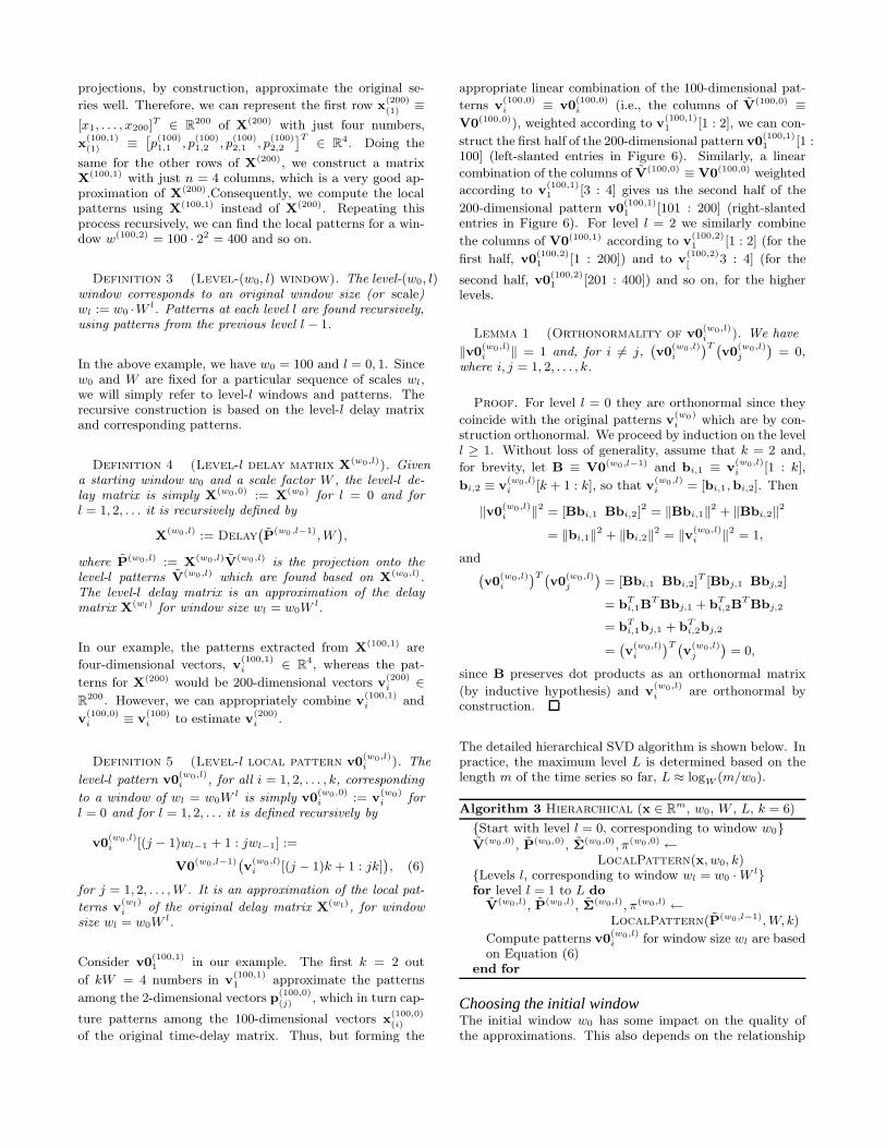
same for the other rows of X(200), we construct a matrixX(100,1) with just n = 4 columns, which is a very good ap-proximation of X(200).Consequently, we compute the localpatterns using X(100,1) instead of X(200). Repeating thisprocess recursively, we can find the local patterns for a win-dow w(100,2) = 100 · 22 = 400 and so on.

Definition 3 (Level-(w0, l) window). The level-(w0, l)window corresponds to an original window size (or scale)wl := w0 ·W

l. Patterns at each level l are found recursively,using patterns from the previous level l − 1.

In the above example, we have w0 = 100 and l = 0, 1. Sincew0 and W are fixed for a particular sequence of scales wl,we will simply refer to level-l windows and patterns. Therecursive construction is based on the level-l delay matrixand corresponding patterns.

Definition 4 (Level-l delay matrix X(w0,l)). Givena starting window w0 and a scale factor W , the level-l de-lay matrix is simply X(w0,0) := X(w0) for l = 0 and forl = 1, 2, . . . it is recursively defined by

X(w0,l) := Delay`

P(w0 ,l−1), W´

,

where P(w0,l) := X(w0,l)V(w0,l) is the projection onto thelevel-l patterns V(w0,l) which are found based on X(w0,l).The level-l delay matrix is an approximation of the delaymatrix X(wl) for window size wl = w0W

l.

In our example, the patterns extracted from X(100,1) are

four-dimensional vectors, v(100,1)i ∈ R

4, whereas the pat-

terns for X(200) would be 200-dimensional vectors v(200)i ∈

R200. However, we can appropriately combine v

(100,1)i and

v(100,0)i ≡ v

(100)i to estimate v

(200)i .

Definition 5 (Level-l local pattern v0(w0,l)i ). The

level-l pattern v0(w0,l)i , for all i = 1, 2, . . . , k, corresponding

to a window of wl = w0Wl is simply v0

(w0,0)i := v

(w0)i for

l = 0 and for l = 1, 2, . . . it is defined recursively by

v0(w0,l)i [(j − 1)wl−1 + 1 : jwl−1] :=

V0(w0,l−1)`

v(w0,l)i [(j − 1)k + 1 : jk]

´

, (6)

for j = 1, 2, . . . , W . It is an approximation of the local pat-

terns v(wl)i of the original delay matrix X(wl), for window

size wl = w0Wl.

Consider v0(100,1)1 in our example. The first k = 2 out

of kW = 4 numbers in v(100,1)1 approximate the patterns

among the 2-dimensional vectors p(100,0)(j) , which in turn cap-

ture patterns among the 100-dimensional vectors x(100,0)(i)

of the original time-delay matrix. Thus, but forming the

appropriate linear combination of the 100-dimensional pat-

terns v(100,0)i ≡ v0

(100,0)i (i.e., the columns of V(100,0) ≡

V0(100,0)), weighted according to v(100,1)1 [1 : 2], we can con-

struct the first half of the 200-dimensional pattern v0(100,1)1 [1 :

100] (left-slanted entries in Figure 6). Similarly, a linear

combination of the columns of V(100,0) ≡ V0(100,0) weighted

according to v(100,1)1 [3 : 4] gives us the second half of the

200-dimensional pattern v0(100,1)1 [101 : 200] (right-slanted

entries in Figure 6). For level l = 2 we similarly combine

the columns of V0(100,1) according to v(100,2)1 [1 : 2] (for the

first half, v0(100,2)1 [1 : 200]) and to v

(100,2)

[3 : 4] (for the

second half, v0(100,2)1 [201 : 400]) and so on, for the higher

levels.

Lemma 1 (Orthonormality of v0(w0,l)i ). We have

‖v0(w0,l)i ‖ = 1 and, for i 6= j,

`

v0(w0,l)i

´T `

v0(w0,l)j

´

= 0,where i, j = 1, 2, . . . , k.

Proof. For level l = 0 they are orthonormal since they

coincide with the original patterns v(w0)i which are by con-

struction orthonormal. We proceed by induction on the levell ≥ 1. Without loss of generality, assume that k = 2 and,

for brevity, let B ≡ V0(w0,l−1) and bi,1 ≡ v(w0,l)i [1 : k],

bi,2 ≡ v(w0,l)i [k + 1 : k], so that v

(w0,l)i = [bi,1, bi,2]. Then

‖v0(w0,l)i ‖2 = [Bbi,1 Bbi,2]

2 = ‖Bbi,1‖2 + ‖Bbi,2‖

2

= ‖bi,1‖2 + ‖bi,2‖

2 = ‖v(w0,l)i ‖2 = 1,

and`

v0(w0,l)i

´T `

v0(w0,l)j

´

= [Bbi,1 Bbi,2]T [Bbj,1 Bbj,2]

= bTi,1B

T Bbj,1 + bTi,2B

T Bbj,2

= bTi,1bj,1 + bT

i,2bj,2

=`

v(w0,l)i

´T `

v(w0,l)j

´

= 0,

since B preserves dot products as an orthonormal matrix

(by inductive hypothesis) and v(w0,l)i are orthonormal by

construction.

The detailed hierarchical SVD algorithm is shown below. Inpractice, the maximum level L is determined based on thelength m of the time series so far, L ≈ logW (m/w0).

Algorithm 3 Hierarchical (x ∈ Rm, w0, W , L, k = 6)

{Start with level l = 0, corresponding to window w0}

V(w0,0), P(w0,0), Σ(w0,0), π(w0,0) ←LocalPattern(x, w0, k)

{Levels l, corresponding to window wl = w0 ·Wl}

for level l = 1 to L doV(w0,l), P(w0 ,l), Σ(w0,l), π(w0,l) ←

LocalPattern(P(w0,l−1), W, k)

Compute patterns v0(w0,l)i for window size wl are based

on Equation (6)end for

Choosing the initial windowThe initial window w0 has some impact on the quality ofthe approximations. This also depends on the relationship

of k to w0 (the larger k is, the better the approximation

and if k = w0 then P(w0,1) = X(w0), i.e., no informationis discarded at the first level). However, we want k to berelatively small since, as we will see, it determines the buffer-ing requirements of the streaming approach. Hence, we fixk = 6. We found that this simple choice works well forreal-world sequences, but we could also use energy-basedthresholding [18], which can be done incrementally.

If w0 is too small, then we discard too much of the variancetoo early. If w0 is unnecessarily big, this increases bufferingrequirements and the benefits of the hierarchical approachdiminish. In practice, a good compromise is a value in therange 10 ≤ w0 ≤ 20.

Finally, out of the six patterns we keep per level, the firsttwo or three are of interest and reported to the user, asexplained in Section 4. The remaining are kept to ensurethat X(w0,l) is a good approximation of X(wl).

Choosing the scalesAs discussed in Section 4.1, if there is a sharp drop of π(T ) atwindow w = T , then we will also observe drops at multiplesw = iT , i = 2, 3, . . .. Therefore, we choose a few differentstarting windows w0 and scale factors W that are relativelyprime to each other. In practice, the following set of threechoices is sufficient to quickly zero in on the best windowsand the associated optimal local patterns:

k = 6 and (w0, W ) ∈ {(9, 2), (10, 2), (15, 3)}

ComplexityFor a total of L ≈ logW (t/w0) = O(log t) levels we have to

compute the first k singular values and vectors of X(w0,l) ∈

Rt/(w0W l)×Wk, for l = 1, 2, . . .. A batch SVD algorithm

requires time O`

k · (Wk)2 · tw0W l

´

, which is O`

W2k2tW l

´

since

k < w0. Summing over l = 1, . . . , L, we get O(W 2k2t).Finally, for l = 0, we need O

`

k · w20

tw0

´

= O(kw0t). Thus,

the total complexity is O(W 2k2t + kw0t). Since W and w0

are fixed, we finally have the following

Lemma 2 (Batch hierarchical complexity). The to-tal time for the hierarchical approach is O(k2t), i.e., linearwith respect to the time series length.

This is a big improvement over the O(t3k) time of the non-hierarchical approach. However, we still need to buffer allthe points. We address this problem in the next section.

6. STREAMING COMPUTATIONIn this section we explain how to perform the necessary com-putations in an incremental, streaming fashion. We designedour models precisely to allow this step. The main idea is thatwe recursively invoke only one iteration of each loop in In-crementalSVD (for LocalPattern) and in Hierarchi-cal, as soon as the necessary number of points has arrived.Subsequently, we can discard these points and proceed withthe next non-overlapping window.

500 1000 1500 2000 25000

50

100

150

200

250Sunspot

Time (weeks)

(a) Sunspot time series.

20 40 60 80100120−0.2

−0.1

0

0.1

0.2First pattern (basis)

Time (1..134)20 40 60 80100120

−0.2

−0.1

0

0.1

0.2Second pattern (basis)

Time (1..134)

(b) Patterns (batch, non-hierarchical).

20 40 60 80 100 120−0.2

−0.1

0

0.1

0.2Second pattern (hierarchical, streaming)

Time (1..144)20 40 60 80 100 120

−0.2

−0.1

0

0.1

0.2First pattern (hierarchical, streaming)

Time (1..144)

(c) Patterns (streaming, hierarchical).

Figure 7: Sunspot, best selected window (about 11years) and corresponding representative trends.

Modifying LocalPatternWe buffer consecutive points of x (or, in general, rows of X)

until we accumulate w of them, forming one row of X(w). Atthat point, we can perform one iteration of the outer loopin IncrementalSVD to update all k local patterns. Then,we can discard the w points (or rows) and proceed with thenext w. Also, since on higher levels the number of pointsfor SVD may be small and close to k, we may choose toinitially buffer just the first k rows of X(w) and use them tobootstrap the SVD estimates, which we subsequently updateas described.

Modifying HierarchicalFor level l = 0 we use the modified LocalPattern on theoriginal series, as above. However, we also store the k pro-jections onto the level-0 patterns. We buffer W consecutivesets of these projections and as soon as kW values accumu-late, we update the k local patterns for level l = 1. Then wecan discard the kW projections from level-0, but we keepthe k level-1 projections. We proceed in the same way forall other levels l ≥ 2.

ComplexityCompared to the batch computation, we need O

`

k ·Wk ·t

w0W l

´

= O`

ktW l−1

´

time to compute the first k singular

values and vectors of X(w0,l) for l = 1, 2, . . .. For l = 0we need O

`

k · w0 ·t

w0

´

= O(kt) time. Summing over l =

0, 1, . . . , L we get O(kt). With respect to space, we needto buffer w0 points for l = 0 and Wk points for each ofthe remaining L = O(log t) levels, for a total of O(k log t).Therefore, we have the following

Lemma 3 (Streaming, hierarchical complexity).Amortized cost is O(k) per incoming point and total spaceis O(k log t).

Since k = 6, the update time is constant per incoming pointand the space requirements grow logarithmically with re-spect to the size t of the series. Table 2 summarizes thetime and space complexity for each approach.

Time SpaceNon-hier. Hier. Non-hier. Hier

Batch O(t3k) O(tk2) all allIncremental O(t2k) O(tk) O(t) O(k log t)

Table 2: Summary of time and space complexity.

7. EXPERIMENTAL EVALUATIONIn this section we demonstrate the effectiveness of our ap-proach on real data. The questions we want to answer are:

1. Do our models for mining locally optimal patterns cor-rectly capture the best window size?

2. Are the patterns themselves accurate and intuitive?

3. How does the quality of the much more efficient, hi-erarchical streaming approach compare to the exactcomputation?

We performed all experiments in Matlab, using the stan-dard functions for batch SVD. Table 3 briefly describes thedatasets we use.

Dataset Size DescriptionAutomobile 59370 Automobile counts on interstateSunspot 2904 Sunspot intensities (years 1755–

1996)Mote 7712 Light intensity data

Table 3: Description of datasets.

Table 4 shows the best windows identified from the powerprofiles. Figure 9 shows the exact power profiles computedusing the batch, non-hierarchical approach and Figure 10shows the power profiles estimated using the streaming, hi-erarchical approach.

Best windowSunspot Mote Auto

Batch 134, 120, 142 156, 166, 314 4000Streaming 144 160, 320 3645

Table 4: Best windows—see also Figures 9 and 10.

Automobile

The results on this dataset were already presented in Sec-tion 1. Our method correctly captures the right window forthe main trend and also an accurate picture of the typicaldaily pattern. The patterns discovered both by the batchand the streaming approach are very close to each other andequally useful.

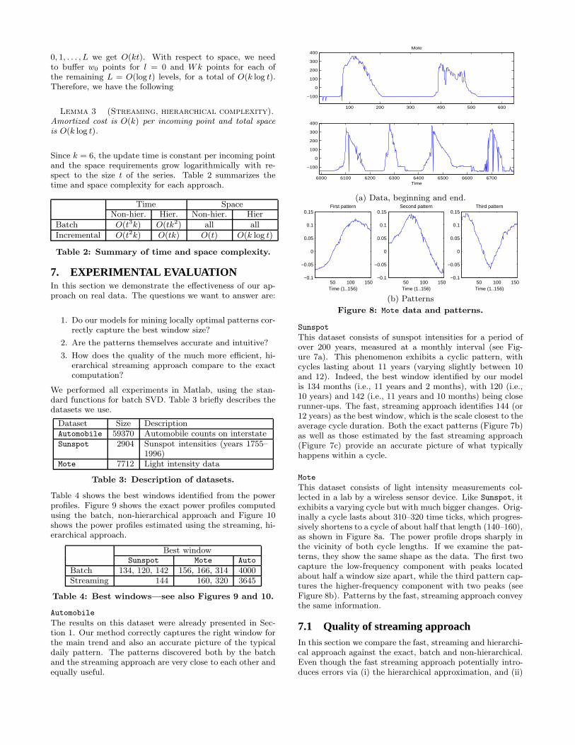
6000 6100 6200 6300 6400 6500 6600 6700

−100

0

100

200

300

400

Time

100 200 300 400 500 600

−100

0

100

200

300

400Mote

(a) Data, beginning and end.

50 100 150−0.1

−0.05

0

0.05

0.1

0.15

Time (1..156)

Third pattern

50 100 150−0.1

−0.05

0

0.05

0.1

0.15

Time (1..156)

Second pattern

50 100 150−0.1

−0.05

0

0.05

0.1

0.15

Time (1..156)

First pattern

(b) Patterns

Figure 8: Mote data and patterns.

Sunspot

This dataset consists of sunspot intensities for a period ofover 200 years, measured at a monthly interval (see Fig-ure 7a). This phenomenon exhibits a cyclic pattern, withcycles lasting about 11 years (varying slightly between 10and 12). Indeed, the best window identified by our modelis 134 months (i.e., 11 years and 2 months), with 120 (i.e.,10 years) and 142 (i.e., 11 years and 10 months) being closerunner-ups. The fast, streaming approach identifies 144 (or12 years) as the best window, which is the scale closest to theaverage cycle duration. Both the exact patterns (Figure 7b)as well as those estimated by the fast streaming approach(Figure 7c) provide an accurate picture of what typicallyhappens within a cycle.

Mote

This dataset consists of light intensity measurements col-lected in a lab by a wireless sensor device. Like Sunspot, itexhibits a varying cycle but with much bigger changes. Orig-inally a cycle lasts about 310–320 time ticks, which progres-sively shortens to a cycle of about half that length (140–160),as shown in Figure 8a. The power profile drops sharply inthe vicinity of both cycle lengths. If we examine the pat-terns, they show the same shape as the data. The first twocapture the low-frequency component with peaks locatedabout half a window size apart, while the third pattern cap-tures the higher-frequency component with two peaks (seeFigure 8b). Patterns by the fast, streaming approach conveythe same information.

7.1 Quality of streaming approachIn this section we compare the fast, streaming and hierarchi-cal approach against the exact, batch and non-hierarchical.Even though the fast streaming approach potentially intro-duces errors via (i) the hierarchical approximation, and (ii)

20 40 60 80 100 120 140 160 180 2000

0.5

1

1.5

2

2.5

3

3.5

4

4.5x 10

−3

X: 134Y: 0.0007202

X: 120Y: 0.001685

X: 120Y: 0.0007322

Sunspot − Power profile

Window size

X: 132Y: 0.001688

k = 1k = 2k = 3

50 100 150 200 250 300 350 4000

0.5

1

1.5

2

2.5

3

3.5

4

4.5

5x 10

−3

X: 314Y: 0.0005688

Window size

Mote − Power profile

k = 1k = 2k = 3

1500 2000 2500 3000 3500 4000 4500 50000

1

2

3

4

5

x 10−5

Window size

Automobile − Power profile

k = 1k = 2k = 3

(a) Sunspot (b) Mote (c) Automobile

Figure 9: Power profiles (non-hierarchical, batch).

the incremental update of the SVD, we show that it stillachieves very good results. The quality should be comparedagainst the significant speedups in Table 5.

Auto Sunspot Mote

Exact 15252 2.0 11.9Streaming 6.5 0.6 1.3Ratio ×2346 ×3.3 ×9.1

Length 59370 2904 7712wmax 5000 400 600

Table 5: Wall-clock times (in seconds). The maxi-mum window wmax for the exact approach and thelength of each series are also shown.

First, the streaming approach correctly zeros in to the bestwindows, which generally correspond to the scale that isclosest to the “true” best windows identified by the exact,batch approach (see Table 4).

Our next goal is to characterize the quality of the patternsthemselves, at the best windows that each approach iden-tifies. To that end, we compare the reconstructions of the

original time series x for the two methods. If v(w∗)i are the

optimal patterns for the best window w∗ (or v0(w∗

0 ,l∗)i for

the streaming approach, with corresponding window w∗l =

w∗0 · W

l∗), we first zero-pad x into x0 so its length is amultiple of w∗, then compute the local pattern projectionsP(w∗) = Delay(x0, w

∗)V(w∗), project back to the original

delay coordinates X(w∗) = P(w∗)`

V(w∗)´T

. Finally, we con-

catenate the rows of X(w∗) into the reconstruction x of x,removing the elements corresponding to the zero-padding.The quality measures we use are

Q := ‖x‖2−‖xstream−x‖2

‖x‖2−‖xexact−x‖2 and C :=|xT

stream xexact|

‖xstream‖ ‖xexact‖.

The first one is a measure of the information retained, withrespect to the total squared error: we compare the frac-tion of information retained by the streaming approach,`

‖x‖2−‖xstream−x‖2´

/‖x‖2, to that retained by the exact

approach,`

‖x‖2−‖xexact−x‖2´

/‖x‖2. The second is simplythe cosine similarity of the two reconstructions, which pe-nalizes small “time shifts” less and more accurately reflectshow close are the overall shapes of the reconstructions.

We use the reconstruction xexact as our baseline. For patterndiscovery, using the original series x itself as the baseline is

undesirable, since that contains noise and other irregularitiesthat should not be part of the discovered patterns.

Finally, we show the cosine similarity of the patterns them-selves, for the best window w∗

l identified by the streamingapproach. This characterizes how close the direction of thehierarchically and incrementally estimated singular vectorsis to the direction of the “true” singular vectors. Table 6shows the results. Figures 2 and 7 allow visual compari-son of the patterns (at slightly different best windows). Insummary, the streaming approach’s patterns capture all theessential information, while requiring 1–4 orders of magni-tude less time and 1–2 orders of magnitude less space.

Dataset Auto Sunspot Mote

Quality ratio 0.97 0.89 0.84Cosine 0.98 0.94 0.89

Pattern 1.00 0.99 0.89similarity 0.85 0.93 0.75(cosine) 0.80 0.94 0.93

Table 6: Batch non-hierarchical vs. streaming hier-archical (k = 3, best window from Table 4).

8. RELATED WORKInitial work on time series representation [1, 11] uses theFourier transform. Even more recent work uses fixed, prede-termined bases or approximating functions. APCA [4] andother similar approaches approximate the time series withpiecewise constant or linear functions. DAWA [14] combinesthe DCT and DWT. However, all these approaches focus oncompressing the time series for indexing purposes, and noton pattern discovery.

AWSOM [24] first applies the wavelet transform. As theauthors observe, just a few wavelet coefficients do not cap-ture all patterns in practice, so AWSOM subsequently cap-tures trends by fitting a linear auto-regressive model at eachtime scale. In contrast, our approach learns the best set oforthogonal bases, while matching the space and time com-plexity of AWSOM. Finally, it is difficult to apply waveletson exponential-size windows that are not powers of two.

The work in [19] proposes a multi-resolution clustering schemefor time series data. It uses the average coefficients (lowfrequencies) of the wavelet transform to perform k-meansclustering and progressively refines the clusters by incor-

50 100 150 200 250 300 350 4000

1

2

3

4

x 10−3

X: 144Y: 0.001437

X: 288Y: 0.0006763

Window size

Sunspot − Power profile (Hierarchical, Streaming)

k = 1k = 2

100 200 300 400 5000.5

1

1.5

2

2.5

3

3.5

4

4.5

x 10−3

X: 160Y: 0.001539

X: 320Y: 0.001649

Window size

Mote − Power profile (Hierarchical, Streaming)

k = 1k = 2

500 1000 1500 2000 2500 3000 3500 4000 4500 5000

10−4

10−3

X: 3645Y: 3.123e−005

Window size

(lo

g)

Auto − Power profile (Hierarchical, Streaming)

k = 1k = 2

(a) Sunspot (b) Mote (c) Automobile

Figure 10: Power profiles (hierarchical, streaming).

porating higher-level, detail coefficients. This approach re-quires much less time for convergence, compared to operat-ing directly on the very high dimension of the original series.However, the focus here is on clustering multiple time series,rather than discovering local patterns.

The problem of principal components analysis (PCA) andSVD on streams has been addressed in [25] and [13]. Again,both of these approaches focus on discovering linear corre-lations among multiple streams and on applying these cor-relations for further data processing and anomaly detection[25], rather than discovering optimal local patterns at multi-ple scales. Also related to these is the work of [8] which usesa different formulation of linear correlations and focuses oncompressing historical data, mainly for power conservationin sensor networks. Finally, the work in [2] proposes an ap-proach to combine segmentation of multidimensional serieswith dimensionality reduction. The reduction is on the seg-ment representatives and it is performed across dimensions(similar to [25]), not along time, and the approach is notapplicable to streams.

The seminal work of [7] for rule discovery in time series isbased on sequential patterns extracted after a discretizationstep. Other work has also focused on finding representa-tive trends [17]. A representative trend is a subsequence ofthe time series that has the smallest sum of distances fromall other subsequences of the same length. The proposedmethod employs random projections and FFT to quicklycompute the sum of distances. This does not apply directlyto streams and it is not easy to extend, since each sectionhas to be compared to all others. Our approach is com-plementary and could conceivably be used in place of theFFT in this setting. Related to representative trends aremotifs [26, 6]. Intuitively, these are frequently repeated sub-sequences, i.e., subsequences of a given length which match(in terms of some distance and a given distance threshold)a large number of other subsequences of the same time se-ries. More recently, vector quantization has been used fortime series compression [21, 20]. The first focuses on findinggood-quality and intuitive distance measures for indexingand similarity search and is not applicable to streams, whilethe second focuses on reducing power consumption for wire-less sensors and not on pattern discovery. Finally, otherwork on stream mining includes approaches for periodicity[10] and periodic pattern [9] discovery.

Approaches for regression on time series and streams include[5] and amnesic functions [23]. Both of these estimate thebest fit of a given function (e.g., linear or low-degree polyno-mial), they work by merging the estimated fit on consecutivewindows and can incorporate exponential-size time windowsplacing less emphasis on the past. However, both of theseapproaches employ a fixed, given set of approximating func-tions. Our approach might better be described as agnostic,rather than amnesic.

A very recent and interesting application of the same princi-ples is on correlation analysis of complex time series throughchange-point scores [16]. Finally, related ideas have beenused in other fields, such as in image processing for im-age denoising [22, 15] and physics/climatology for nonlinearprediction in phase space [35]. However, none of these ap-proaches address incremental computation in streams. Moregenerally, the potential of this general approach has not re-ceived attention in time series and stream processing liter-ature. We demonstrate that its power can be harnessed atvery small cost, no more than that of the widely used wavelettransform.

9. CONCLUSIONWe introduce a method to that can learn the key trends ina time series. Our main contributions are:

• We introduce the notion of optimal local patterns intime series.

• We show how to extract trends at multiple time scales.

• We propose a criterion which allows us to choose thebest window sizes from the data.

• We introduce an approach to perform all of the aboveincrementally, in a streaming setting.

Furthermore, our approach can be easily extended to an en-semble of multiple time series, unlike fixed-basis methods(e.g., FFT, SFT or DWT), and also to deal with missingvalues. Besides providing insight about the behavior of thetime series, the discovered patterns can also be used to facil-itate further data processing. In fact, our approach can beused anywhere a fixed-basis orthonormal transform wouldbe used.

Especially in a streaming setting, it makes more sense tofind the best bases and project only onto these, rather thanuse an a priori determined set of bases and then try to find

the “best” coefficients. However, computing these bases in-crementally and efficiently is a challenging problem. Ourstreaming approach achieves 1-4 orders of magnitude im-provement in time and space over the exact, batch approach.Its time and space requirements are comparable to previousmulti-scale pattern mining approaches on streams [24, 23, 5],while it produces significantly more concise and informativepatterns, without any prior knowledge about the data.

REFERENCES[1] R. Agrawal, C. Faloutsos, and A. N. Swami. Efficient

similarity search in sequence databases. In FODO,1993.

[2] E. Bingham, A. Gionis, N. Haiminen, H. Hiisila,H. Mannila, and E. Terzi. Segmentation and dimen-sionality reduction. In SDM, 2006.

[3] M. Brand. Fast online SVD revisions for lightweightrecommender systems. In SDM, 2003.

[4] K. Chakrabarti, E. Keogh, S. Mehotra, and M. Pazzani.Localy adaptive dimensionality reduction for indexinglarge time series databases. TODS, 27(2), 2002.

[5] Y. Chen, G. Dong, J. Han, B. W. Wah, and J. Wang.Multi-dimensional regression analysis of time-seriesdata streams. In VLDB, 2002.

[6] B. Chiu, E. Keogh, and S. Lonardi. Probabilistic dis-covery of time series motifs. In KDD, 2003.

[7] G. Das, K.-I. Lin, H. Mannila, G. Renganathan, andP. Smyth. Rule discovery from time series. In KDD,1998.

[8] A. Deligiannakis, Y. Kotidis, and N. Roussopoulos.Compressing historical information in sensor networks.In SIGMOD, 2004.

[9] M. G. Elefky, W. G. Aref, and A. K. Elmagarmid. Usingconvolution to mine obscure periodic patterns in onepass. In EDBT, 2004.

[10] M. G. Elefky, W. G. Aref, and A. K. Elmagarmid.WARP: Time warping for periodicity detection. InICDM, 2005.

[11] C. Faloutsos, M. Ranganathan, and Y. Manolopoulos.Fast subsequence matching in time-series databases. InSIGMOD, 1994.

[12] M. Ghil, M. Allen, M. Dettinger, K. Ide, D. Kon-drashov, M. Mann, A. Robertson, A. Saunders,Y. Tian, F. Varadi, and P. Yiou. Advanced spectralmethods for climatic time series. Rev. Geophys., 40(1),2002.

[13] S. Guha, D. Gunopulos, and N. Koudas. Correlatingsynchronous and asynchronous data streams. In KDD,2003.

[14] M.-J. Hsieh, M.-S. Chen, and P. S. Yu. IntegratingDCT and DWT for approximating cube streams. InCIKM, 2005.

[15] A. Hyvarinen, P. Hoyer, and E. Oja. Sparse codeshrinkage for image denoising. In WCCI, 1998.

[16] T. Ide and K. Inoue. Knowledge discovery from het-erogeneous dynamic systems using change-point corre-lations. In SDM, 2005.

[17] P. Indyk, N. Koudas, and S. Muthukrishnan. Identi-fying representative trends in massive time series datasets using sketches. In VLDB, 2000.

[18] I. T. Jolliffe. Principal Component Analysis. Springer,2nd edition, 2002.

[19] J. Lin, M. Vlachos, E. J. Keogh, and D. Gunopulos. It-erative incremental clustering of time series. In EDBT,2004.

[20] S. Lin, D. Gunopulos, V. Kalogeraki, and S. Lonardi.A data compression technique for sensor networks withdynamic bandwidth allocation. In TIME, 2005.

[21] V. Megalooikonomou, Q. Wang, G. Li, and C. Falout-sos. A multiresolution symbolic representation of timeseries. In ICDE, 2005.

[22] D. D. Muresan and T. W. Parks. Adaptive principalcomponents and image denoising. In ICIP, 2003.

[23] T. Palpanas, M. Vlachos, E. J. Keogh, D. Gunopu-los, and W. Truppel. Online amnesic approximationof streaming time series. In ICDE, 2004.

[24] S. Papadimitriou, A. Brockwell, and C. Faloutsos.Adaptive, unsupervised stream mining. VLDB J.,13(3), 2004.

[25] S. Papadimitriou, J. Sun, and C. Faloutos. Streamingpattern discovery in multiple time series. In VLDB,2005.

[26] P. Patel, E. Keogh, J. Lin, and S. Lonardi. Miningmotifs in massive time series databases. In ICDM, 2002.

[27] D. B. Percival and A. T. Walden. Wavelet Methods forTime Series Analysis. Cambridge Univ. Press, 2000.

[28] M. R. Portnoff. Short-time Fourier analysis of sampledspeech. IEEE Trans. ASSP, 29(3), 1981.

[29] G. Strang. Linear Algebra and Its Applications. BrooksCole, 3rd edition, 1998.

[30] W. Sweldens and P. Schroder. Building your ownwavelets at home. In Wavelets in Computer Graphics,pages 15–87. SIGGRAPH Course notes, 1996.

[31] M. E. Tipping and C. M. Bishop. Probabilistic principalcomponent analysis. J. Royal Stat. Soc. B, 61(3), 1999.

[32] J. Villasenor, B. Belzer, and J. Liao. Wavelet filterevaluation for image compression. IEEE Trans. Im.Proc., 4(8), 1995.

[33] M. Vlachos, C. Meek, Z. Vagena, and D. Gunopulos.Identifying similarities, periodicities and bursts for on-line search queries. In SIGMOD, 2004.

[34] B. Yang. Projection approximation subspace tracking.IEEE Trans. Sig. Proc., 43(1), 1995.

[35] P. Yiou, D. Sornette, and M. Ghil. Data-adaptivewavelets and multi-scale singular-spectrum analysis.Physica D, 142, 2000.