optimal particle filters for tracking a time-varying harmonic or

4598 IEEE TRANSACTIONS ON SIGNAL PROCESSING, VOL. 56, NO. 10, OCTOBER 2008

Optimal Particle Filters for Tracking a Time-VaryingHarmonic or Chirp Signal

Efthimios E. Tsakonas, Nicholas D. Sidiropoulos, Senior Member, IEEE, and Ananthram Swami, Fellow, IEEE

Abstract—We consider the problem of tracking the time-varying(TV) parameters of a harmonic or chirp signal using particle fil-tering (PF) tools. Similar to previous PF approaches to TV spec-tral analysis, we assume that the model parameters (complex am-plitude, frequency, and frequency rate in the chirp case) evolve ac-cording to a Gaussian AR(1) model; but we concentrate on the im-portant special case of a single TV harmonic or chirp. We show thatthe optimal importance function that minimizes the variance of theparticle weights can be computed in closed form, and develop pro-cedures to draw samples from it. We further employ Rao–Black-wellization to come up with reduced-complexity versions of the op-timal filters. The end result is custom PF solutions that are consid-erably more efficient than generic ones, and can be used in a broadrange of important applications that involve a single TV harmonicor chirp signal, e.g., TV Doppler estimation in communications,and radar.

Index Terms—carrier frequency offset, chirp, Doppler, particlefiltering, polynomial phase, radar, time-frequency analysis, time-varying harmonic, tracking.

I. INTRODUCTION AND DATA MODEL

S PECTRAL analysis and time-frequency analysis are coretools in signal processing research (e.g., [6] and [17]).

Time-varying (TV) spectra arise in a broad range of importantapplications: from speech, to radar, to wireless communica-tions.

TV spectral analysis tools range from basic nonparametricapproaches such as the spectrogram, to the Wigner–Ville andother time-frequency distributions, and on to parametric onessuch as polynomial basis expansion models, and TV line spectramixture models.

Line spectra mixtures (whether stationary or TV) entail a non-linear observation equation, which complicates parameter esti-mation. When the evolution of model parameters can be cap-

Manuscript received April 2, 2007; revised May 7, 2008. First publishedJune 20, 2008; current version published September 17, 2008. The associateeditor coordinating the review of this manuscript and approving it for publica-tion was Dr. Antonio Napolitano. An earlier version of part of this work ap-pears in conference form in the Proceedings of the IEEE Nonlinear StatisticalSignal Processing Workshop (NSSPW), Corpus Christi College, Cambridge,U.K., September 13–15, 2006. Supported in part by the Army Research Labora-tory (ARL) through participation in the ARL Collaborative Technology Alliance(ARL-CTA) for Communications and Networks under Cooperative AgreementDADD19-01-2-0011, and in part by ARO under ERO Contract N62558-03-C-0012.

E. E. Tsakonas and N. D. Sidiropoulos are with the Department of Elec-tronic and Computer Engineering, Technical University of Crete, 73100Chania—Crete, Greece (e-mail: [email protected]; [email protected]).

A. Swami is with the Army Research Laboratory, Adelphi, MD 20783 USA(e-mail: [email protected]).

Digital Object Identifier 10.1109/TSP.2008.927462

tured in state-space form, particle filtering (PF) tools becomeparticularly appealing for tracking the model parameters, andthere have been several contributions in the recent literaturedealing with PF approaches to TV spectrum estimation [1], [2],[5], [12], [13], [21].

PF algorithms for tracking time-varying phase and amplitudeare considered in [2]. While it is possible to derive instanta-neous frequency and frequency rate estimates by taking succes-sive phase differences, such an indirect approach is ad hoc andproblematic in practice.

For a multicomponent TV harmonic mixture model, PF ap-proaches have been pursued in [1] and [12]. In [1], the evolutionof harmonic parameters (frequencies, complex amplitudes, pos-sibly also decay rates) follows a moving average (MA) model,the measurement follows a Gaussian TV autoregressive (TVAR)model, and an improved auxiliary particle filtering algorithm isapplied to track the parameters. In [12], a Gaussian random walkmodel is employed for the evolution of the parameters, and anunscented PF algorithm is adapted to track them. The use of tem-poral slices of the spectrogram in the measurement equation of[12] limits the attainable time-frequency resolution. Follow-upwork in [13] uses the spectrogram to design the importance dis-tribution for the frequency, the underlying assumption being thatfrequency is locally constant (see also [5] and [21] for an appli-cation of TVAR modeling to the enhancement of speech sig-nals).

Gaussian AR models of the evolution of harmonic mixtureparameters are plausible and convenient in many situa-tions—e.g., they can capture smoothness due to inertia or otherphysical constraints. Following [1] and [12], we also assumethat the parameters (complex amplitude, frequency, and fre-quency rate in the chirp case) evolve according to a GaussianAR(1) model; but we concentrate on the important special caseof a single TV harmonic or chirp signal.

The specific model we use for a TV harmonic is as follows.Let denote the state at time , where1

and denote instantaneous frequency and complex am-plitude. The state is assumed to evolve according to the fol-lowing AR(1) model:

where is 2 2 diagonal, , with

equal to (with typically small, e.g., ).The process noise sequence is independent and identically dis-

1� � � � , where � is the instantaneous frequency of the underlyingcontinuous-time signal at time � � �� , and � is the sampling period. We areinterested in estimating � . There is potential for aliasing due to sampling, butwe are interested in tracking small offsets and slow drifts.

1053-587X/$25.00 © 2008 IEEE

Authorized licensed use limited to: TECHNICAL UNIVERSITY OF CRETE. Downloaded on November 21, 2008 at 04:27 from IEEE Xplore. Restrictions apply.

TSAKONAS et al.: OPTIMAL PARTICLE FILTERS FOR TRACKING A TV HARMONIC OR CHIRP SIGNAL 4599

tributed (i.i.d.). The process noise vector at time consists oftwo independent random variables with the following marginalstatistics:

where , stand for the (real) normal and circularly sym-metric complex normal distribution, respectively. The measure-ments are related to the state via the measurement equation

where denotes i.i.d. measurement noise.Given a sequence of observations , the problem of

interest is to estimate the sequence of posterior densities, that is, . Given , one

can estimate via the associated (posterior) mean.For the above model (and its extension to a TV chirp), we

show that the optimal importance function (that minimizes thevariance of the particle weights) can be computed in closedform, and develop procedures to draw samples from it. Com-puting the optimal important function in closed form was notpossible for the models in [1], [2], [5], [12], [13], and [21].We further employ Rao–Blackwellization to come up with re-duced-complexity versions of the optimal filters. The resultingfilters are considerably more efficient than generic ones, and canbe applied in a broad range of applications in digital communi-cations and radar, such as tracking Doppler frequency and fre-quency rate drift due to irregular motion.

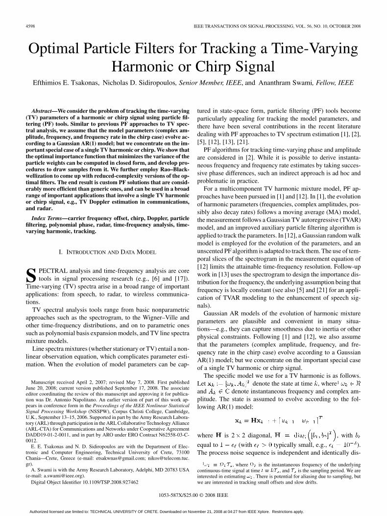
The above model may appear benign in its simplicity, but itis not. First, the measurement nonlinearity is severe. Second, incontrast to a general time-varying phase model, we explicitlymodel variations in instantaneous frequency. That is, we con-strain the phase to be an affine function of time , but allow time-varying jitter in the slope and the offset. These are precisely theparameters of interest in wireless communications applications.To appreciate the nature of the model, the following illustra-tion is instructive. Fig. 1 depicts a sample path of the evolutionof the frequency variable, generated using ,

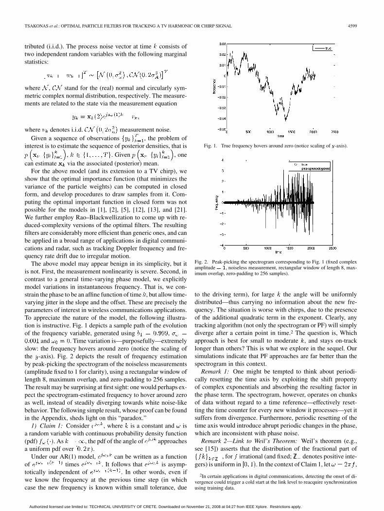
and . Time variation is—purposefully—extremelyslow: the frequency hovers around zero (notice the scaling ofthe -axis). Fig. 2 depicts the result of frequency estimationby peak-picking the spectrogram of the noiseless measurements(amplitude fixed to 1 for clarity), using a rectangular window oflength 8, maximum overlap, and zero-padding to 256 samples.The result may be surprising at first sight: one would perhaps ex-pect the spectrogram-estimated frequency to hover around zeroas well, instead of steadily diverging towards white noise-likebehavior. The following simple result, whose proof can be foundin the Appendix, sheds light on this “paradox.”

1) Claim 1: Consider , where is a constant and isa random variable with continuous probability density function(pdf) . As , the pdf of the angle of approachesa uniform pdf over .

Under our AR(1) model, can be written as a functionof times . It follows that is asymp-totically independent of . In other words, even ifwe know the frequency at the previous time step (in whichcase the new frequency is known within small tolerance, due

Fig. 1. True frequency hovers around zero (notice scaling of �-axis).

Fig. 2. Peak-picking the spectrogram corresponding to Fig. 1 (fixed complexamplitude � �, noiseless measurement, rectangular window of length 8, max-imum overlap, zero-padding to 256 samples).

to the driving term), for large the angle will be uniformlydistributed—thus carrying no information about the new fre-quency. The situation is worse with chirps, due to the presenceof the additional quadratic term in the exponent. Clearly, anytracking algorithm (not only the spectrogram or PF) will simplydiverge after a certain point in time.2 The question is, Whichapproach is best for small to moderate , and stays on-tracklonger than others? This is what we explore in the sequel. Oursimulations indicate that PF approaches are far better than thespectrogram in this context.

Remark 1: One might be tempted to think about periodi-cally resetting the time axis by exploiting the shift propertyof complex exponentials and absorbing the resulting factor inthe phase term. The spectrogram, however, operates on chunksof data without regard to a time reference—effectively reset-ting the time counter for every new window it processes—yet itsuffers from divergence. Furthermore, periodic resetting of thetime axis would introduce abrupt periodic changes in the phase,which are inconsistent with phase noise.

Remark 2—Link to Weil’s Theorem: Weil’s theorem (e.g.,see [15]) asserts that the distribution of the fractional part of

, for irrational (and fixed; denotes positive inte-gers) is uniform in . In the context of Claim 1, let ,

2In certain applications in digital communications, detecting the onset of di-vergence could trigger a cold start at the link level to reacquire synchronizationusing training data.



and denote fractional part. Then .The pdf of has been assumed continuous, and thus a realiza-tion of will be irrational with probability one. Weil’s theoremthen shows that the sample (empirical) distribution of the angleof for a fixed realization of and all is uniform over

. In contrast, Claim 1 asserts that the ensemble distribu-tion of the angle of is (approximately) uniform overfor a fixed large and random with continuous pdf. So, Weil’sTheorem applies to sample path averages, whereas Claim 1 toasymptotic ensemble averages. The ensemble distribution con-verges to the sample path distribution for large ; this isan ergodic property of the random process . Interestingly,Claim 1 does not require to be integer.

II. PARTICLE FILTERING

Particle filtering has emerged as an important sequential stateestimation method for stochastic nonlinear and/or non-Gaussianstate-space models, for which it provides a powerful alternativeto the commonly used extended Kalman filter. See [3], [8], and[9] for recent tutorial overviews.

In particle filtering, continuous distributions are approxi-mated by discrete random measures, comprising “particles”and associated weights. That is, a continuous distribution( is a time index) is approximated as

where denotes the Dirac delta functional, is the thparticle (location) for time and is the associated weight.A useful simplification stemming from this approximation isthat the computation of pertinent expectations and conditionalprobabilities reduces to summation, as opposed to integration.While this can also be accomplished via direct discretizationover a fixed grid, the use of a random measure affords flexibilityin adapting the particle locations to better fit the distribution ofinterest.

If we aim for an online filtering algorithm, in which the stateat time should be estimated from measurements up to andincluding time , the key distribution of interest is the pos-terior density . The basic idea of particle fil-tering, then, is to begin with a random measure approximationof the initial state distribution, and, as measurements becomeavailable, derive updated random measure approximations of

, . That is, we seek random mea-sure approximations

from which the state at time can be estimated via the asso-ciated posterior mean . In particle fil-

tering, the updates—the derivation of from

—are based on the Bayes rule [3], [8].A random measure approximation comprises two compo-

nents: the particles (locations) and the associated weights. If

we could sample from the sought posterior ,then all particle weights would have been equal. Unfortunately,such direct sampling is not possible in most cases, and thuswe resort to sampling from a so-called importance functionthat “resembles” the desired posterior, and from which samplescan be drawn with relative ease. The mismatch between thesought density and the importance function is compensated inthe calculation of weights, chosen proportional to their ratioevaluated at each particle [3], [8].

Different types of particle filters may be applied to agiven state-space model. The various particle filters primarilydiffer in the choice of importance (or, proposal) function.Different importance functions yield different estimation per-formance—complexity tradeoffs. Perhaps the most intuitivechoice of importance function is the prior importance function

; i.e., the th particle is updated by propagatingit through the state-evolution part of the system. This is acommon choice, for simplicity considerations. The drawback isthat particles evolve without regard to the latest measurement,which only comes into play in the ensuing weight update. Whenusing the prior importance function, the weight update at timeinstant is given by , followed bynormalization to enforce .

Regardless of the particular importance function employed, acommon problem in particle filtering is degeneracy: the weightsof all but a few particles tend to become negligible after a fewiterations [3], [8]. Degeneracy can be detected via degeneracymeasures, and mitigated via resampling techniques [3], [8]. Re-sampling the discrete measure replicates particles with largeweights and removes those with negligible weights. All par-ticle weights become equal after resampling. There exist severalcomputationally efficient resampling schemes that canbe used to avoid the quadratic cost of brute-force resampling[3], [8].

From the viewpoint of minimizing the variance of theweights, the optimal importance function (OIF) is given by [3],[8]

where denotes the th particle at time ,which is computed by plugging the th particle at time intothe OIF above, and drawing a sample from it. The OIF usuallystrikes a better performance—complexity tradeoff than other al-ternatives. There are, however, two difficulties associated withthe use of the OIF. First and foremost, it requires integration tocompute the normalization factor, which is usually intractabledue to nonlinearity. Second, sampling from the optimal impor-tance function is a rather complicated process. Thankfully, forour particular model, it turns out that it is possible to carry outthe integration analytically. This is explained next.

III. OPTIMAL IMPORTANCE FUNCTION: TV HARMONIC CASE

Define a dummy variable , and let. Then [see



the first equation at the bottom of the page]. Letting, , ,

where extracts the angle of its argument, it can be shown3

that

with the multiplicative factor given by

where denotes the modified Bessel function of the firstkind of order . The sum term for is quite interesting. Due tothe negative exponential dependence on , , and the propertiesof modified Bessel functions, it vanishes quickly with and .Given , it is easy to come up with a closed-form upper boundon the truncation error, which is, however, overly conservative.Truncation to 20 terms is adequate in all cases considered in ourexperiments—adding more terms does not affect the results. Weused 100 terms as an extra safety margin in our simulations.

We can use rejection [7, pp. 40–42] to generate samples fromthe optimal importance function [see the last equation at thebottom of the page].

The basic idea of rejection-based sampling can be sum-marized as follows [7, pp. 40–42]. Suppose we wish todraw samples from a density , for which there exists adominating density and a known constant such that

. In practice, we choose to be easyto sample from, and such that is as small as possible. Therejection method then works as follows.

Algorithm 1:

1) Draw a sample from and an independent sampleuniformly distributed in ).

2) Set .3) If , then accept and return ; else reject and go

to Step 1.

3Detailed derivation of this and other results in the paper are available assupplementary material in ieeexplore.

It can be shown that the above rejection method generatessamples from the desired density , and the mean number ofiterations until a sample is accepted is (thus the desire to keep

as small as possible). Furthermore, the distribution of thenumber of trials is geometric with parameter , whichmeans that the probabilities of longer trials decay exponentially[7, p. 42].

Let

and

Using the triangle inequality, it can be shown that a suitabledominating density is

where

For this particular choice of IF and sampling procedure theweight update step is given byand can be carried out before sampling from the optimal impor-tance function (before the particles are propagated to time-step

).

IV. RAO–BLACKWELLIZATION

For our particular state-space model, it is possible to reducethe dimensionality of the problem via a technique known asRao–Blackwellization (see [10], [11], [18], and referencestherein). Conditioned on frequency, our model is AR(1) linearGaussian on the complex amplitude. The basic idea is to exploit



this structure to avoid computing everything with plain MonteCarlo sampling. The particle filter is only used to handle thepurely nonlinear portion of the state-space.

Reference [18] considers a general nonlinear state-spacemodel that contains a conditionally linear part, and works outthe Rao–Blackwellization procedure in detail. Our particularmodel is a special case of the so-called Diagonal Model in [18];however, we use the OIF to draw samples for the nonlinearpart. The choice of importance function is left open in [18]to maintain generality—usually the OIF cannot be computedanalytically.

The desired posterior pdf at time , canbe written as

This factorization enables us to use particles only to approx-imate , which is a one-dimensional pdf;

can then be analytically computed usingthe Kalman filter. For state estimation, a Kalman filter isassociated to each frequency particle, and the conditionalmean filtered estimate of the Kalman filter is used to fill-in the“missing” amplitude dimension.

We use the optimal importance distribution to approximatethe marginal posterior density . The optimalimportance distribution is

Letting ,, , it can be shown

that [see the equation at the bottom of the page] with

The weight update is given by ,with

To generate samples distributed according to, we could employ the transforma-

tion method [7]: this is, after all, a one-dimensional pdf.Still, this requires another integration and some level ofapproximation (the integral cannot be put in closed form). Asan alternative, we found that rejection for this one-dimensionalpdf is far more efficient than in the previous case (whichinvolved three real dimensions), and delivers exact samples,which is a definite advantage relative to other samplingmethods. A common criticism of rejection for real-timeapplications is that it takes a random number of draws perparticle. With as few as 30 to 50 particles, however, varianceis averaged out and the complexity per input measurement isstable enough for our purposes.

Starting from and using the triangle in-equality, it is straightforward to show that a suitable dominatingdensity is the transitional prior . The constantassociated with the accept-reject algorithm becomes

It is interesting to see that sampling from the optimal importancefunction can be implemented by rejection over the transitionalprior, which is commonly used as importance function per se.Pseudo-code for the Rao–Blackwellized optimal filter can befound in Table I.

V. CRAMÉR–RAO LOWER BOUND

The Cramér–Rao lower bound (CRLB) for our model can becomputed using the recursive formula of Tichavsky et al. [20]for the calculation of the Fisher information matrix, . Thestate equation in our particular model is linear, Gaussian; thisallows considerable simplification of the general result in [20],thus yielding

with

and



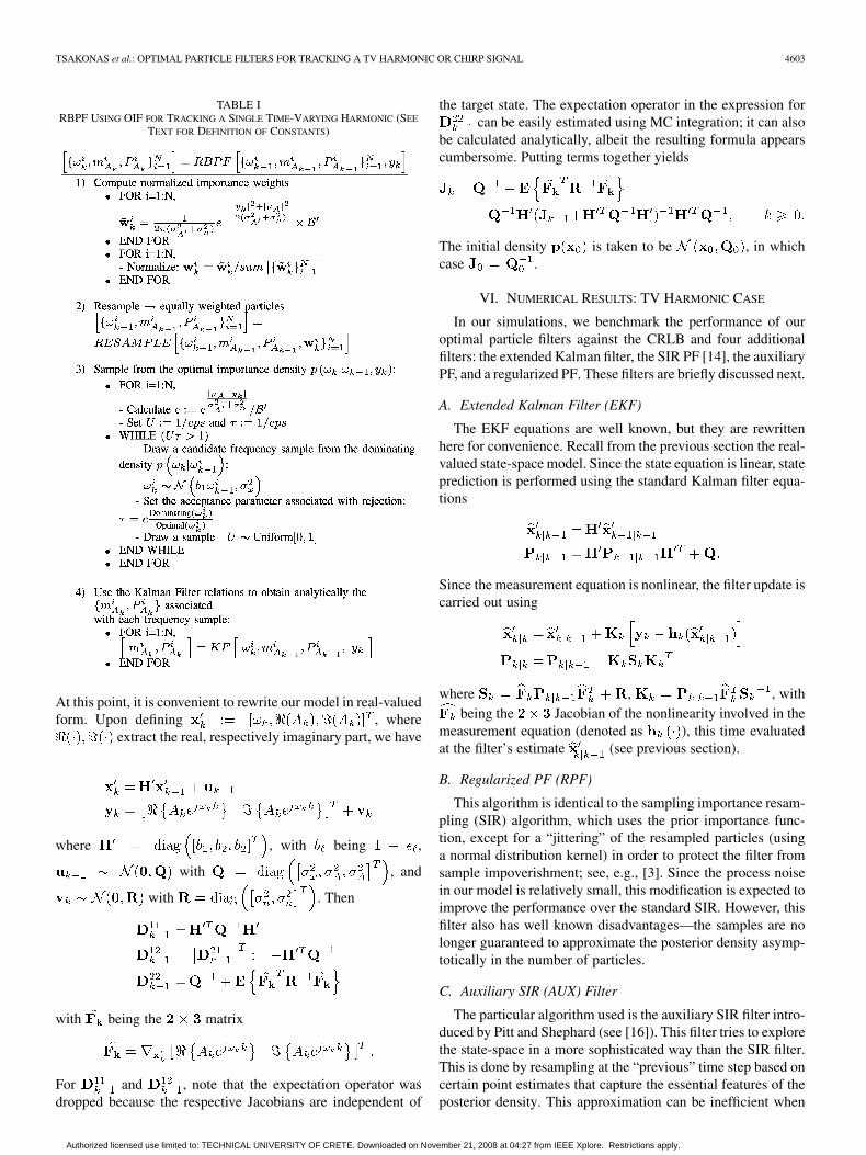
TABLE IRBPF USING OIF FOR TRACKING A SINGLE TIME-VARYING HARMONIC (SEE

TEXT FOR DEFINITION OF CONSTANTS)

At this point, it is convenient to rewrite our model in real-valuedform. Upon defining , where

extract the real, respectively imaginary part, we have

where , with being ,

with , and

with . Then

with being the matrix

For and , note that the expectation operator wasdropped because the respective Jacobians are independent of

the target state. The expectation operator in the expression forcan be easily estimated using MC integration; it can also

be calculated analytically, albeit the resulting formula appearscumbersome. Putting terms together yields

The initial density is taken to be , in whichcase .

VI. NUMERICAL RESULTS: TV HARMONIC CASE

In our simulations, we benchmark the performance of ouroptimal particle filters against the CRLB and four additionalfilters: the extended Kalman filter, the SIR PF [14], the auxiliaryPF, and a regularized PF. These filters are briefly discussed next.

A. Extended Kalman Filter (EKF)

The EKF equations are well known, but they are rewrittenhere for convenience. Recall from the previous section the real-valued state-space model. Since the state equation is linear, stateprediction is performed using the standard Kalman filter equa-tions

Since the measurement equation is nonlinear, the filter update iscarried out using

where , , withbeing the Jacobian of the nonlinearity involved in the

measurement equation (denoted as ), this time evaluatedat the filter’s estimate (see previous section).

B. Regularized PF (RPF)

This algorithm is identical to the sampling importance resam-pling (SIR) algorithm, which uses the prior importance func-tion, except for a “jittering” of the resampled particles (usinga normal distribution kernel) in order to protect the filter fromsample impoverishment; see, e.g., [3]. Since the process noisein our model is relatively small, this modification is expected toimprove the performance over the standard SIR. However, thisfilter also has well known disadvantages—the samples are nolonger guaranteed to approximate the posterior density asymp-totically in the number of particles.

C. Auxiliary SIR (AUX) Filter

The particular algorithm used is the auxiliary SIR filter intro-duced by Pitt and Shephard (see [16]). This filter tries to explorethe state-space in a more sophisticated way than the SIR filter.This is done by resampling at the “previous” time step based oncertain point estimates that capture the essential features of theposterior density. This approximation can be inefficient when



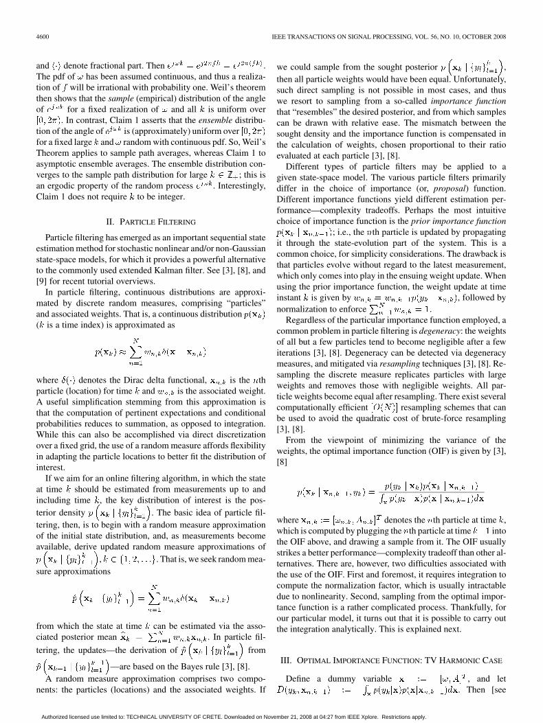
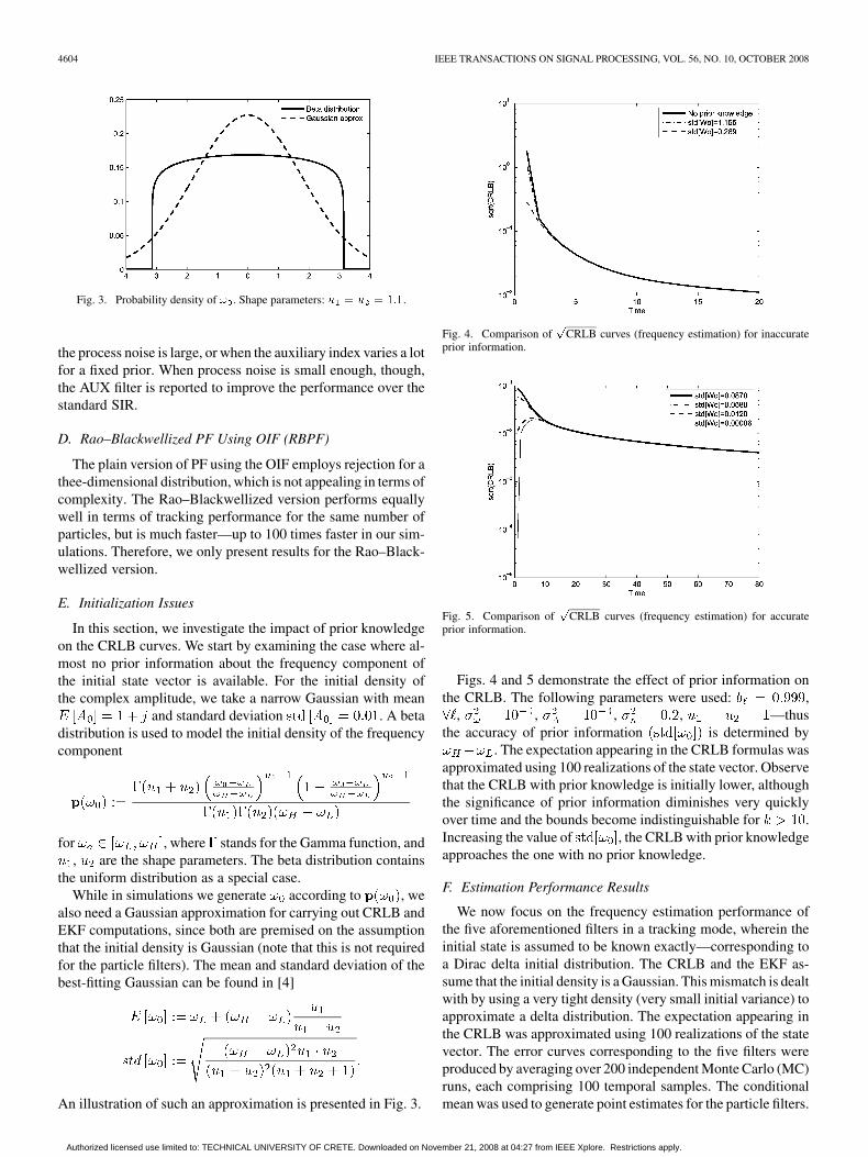
Fig. 3. Probability density of � . Shape parameters: � � � � ��.

the process noise is large, or when the auxiliary index varies a lotfor a fixed prior. When process noise is small enough, though,the AUX filter is reported to improve the performance over thestandard SIR.

D. Rao–Blackwellized PF Using OIF (RBPF)

The plain version of PF using the OIF employs rejection for athee-dimensional distribution, which is not appealing in terms ofcomplexity. The Rao–Blackwellized version performs equallywell in terms of tracking performance for the same number ofparticles, but is much faster—up to 100 times faster in our sim-ulations. Therefore, we only present results for the Rao–Black-wellized version.

E. Initialization Issues

In this section, we investigate the impact of prior knowledgeon the CRLB curves. We start by examining the case where al-most no prior information about the frequency component ofthe initial state vector is available. For the initial density ofthe complex amplitude, we take a narrow Gaussian with mean

and standard deviation . A betadistribution is used to model the initial density of the frequencycomponent

for , where stands for the Gamma function, and, are the shape parameters. The beta distribution contains

the uniform distribution as a special case.While in simulations we generate according to , we

also need a Gaussian approximation for carrying out CRLB andEKF computations, since both are premised on the assumptionthat the initial density is Gaussian (note that this is not requiredfor the particle filters). The mean and standard deviation of thebest-fitting Gaussian can be found in [4]

An illustration of such an approximation is presented in Fig. 3.

Fig. 4. Comparison of�

CRLB curves (frequency estimation) for inaccurateprior information.

Fig. 5. Comparison of�

CRLB curves (frequency estimation) for accurateprior information.

Figs. 4 and 5 demonstrate the effect of prior information onthe CRLB. The following parameters were used: ,

, , , , —thusthe accuracy of prior information is determined by

. The expectation appearing in the CRLB formulas wasapproximated using 100 realizations of the state vector. Observethat the CRLB with prior knowledge is initially lower, althoughthe significance of prior information diminishes very quicklyover time and the bounds become indistinguishable for .Increasing the value of , the CRLB with prior knowledgeapproaches the one with no prior knowledge.

F. Estimation Performance Results

We now focus on the frequency estimation performance ofthe five aforementioned filters in a tracking mode, wherein theinitial state is assumed to be known exactly—corresponding toa Dirac delta initial distribution. The CRLB and the EKF as-sume that the initial density is a Gaussian. This mismatch is dealtwith by using a very tight density (very small initial variance) toapproximate a delta distribution. The expectation appearing inthe CRLB was approximated using 100 realizations of the statevector. The error curves corresponding to the five filters wereproduced by averaging over 200 independent Monte Carlo (MC)runs, each comprising 100 temporal samples. The conditionalmean was used to generate point estimates for the particle filters.



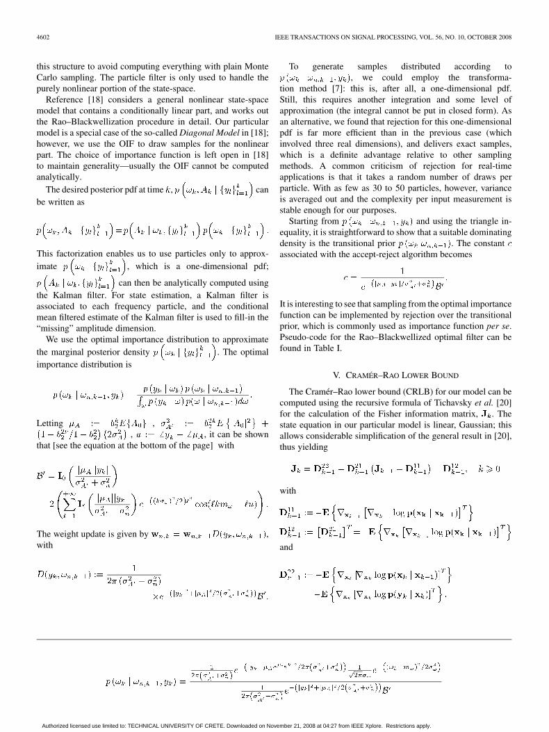
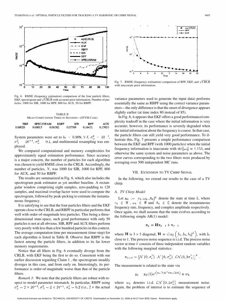
Fig. 6. RMSE (frequency estimation) comparison of the four particle filters,EKF, spectrogram and

�CRLB with accurate prior information. Number of par-

ticles: 1000 for SIR, 1000 for RPF, 800 for AUX, 50 for RBPF.

TABLE IIMEAN COMPUTATION TIMES IN SECONDS—(STVH CASE)

System parameters were set to , , ,, , and multinomial resampling was em-

ployed.We compared computational and memory complexities for

approximately equal estimation performance. Since accuracyis a major concern, the number of particles for each algorithmwas chosen to yield RMSE close to the CRLB. Accordingly, thenumber of particles, , was 1000 for SIR, 1000 for RPF, 800for AUX, and 50 for RBPF.

The results are summarized in Fig. 6, which also includes thespectrogram peak estimator as yet another baseline. A rectan-gular window comprising eight samples, zero-padding to 128samples, and maximal overlap factor were used to compute thespectrogram, followed by peak-picking to estimate the instanta-neous frequency.

It is satisfying to see that the four particles filters and the EKFoperate close to the CRLB, and RBPF in particular performs thatwell with order-of-magnitude less particles. This being a three-dimensional state-space, such good performance with only 50particles is not at all obvious. SIR, RPF and AUX filters performvery poorly with less than a few hundred particles in this context.The average computation time per measurement (time-step) foreach algorithm is listed in Table II. Observe that RBPF is thefastest among the particle filters, in addition to its far lowermemory requirements.

Notice that all filters in Fig. 6 eventually diverge from theCRLB, with EKF being the first to do so. Consistent with ourearlier discussion regarding Claim 1 , the spectrogram steadilydiverges in this case, and from early on. Interestingly, its per-formance is order-of-magnitude worse than that of the particlefilters.

Remark 3: We note that the particle filters are robust with re-spect to model parameter mismatch. In particular, RBPF using

, , (i.e., 2 the actual

Fig. 7. RMSE (frequency estimation) comparison of RPF, EKF, and�

CRLBwith inaccurate prior information.

variance parameters used to generate the input data) performsessentially the same as RBPF using the correct variance param-eters—the only difference is that the onset of divergence appearsslightly earlier (at time index 80 instead of 85).

In Fig. 6, it appears that EKF offers a good performance/com-plexity tradeoff in the case where the initial information is veryaccurate; however, its performance is severely degraded whenthe initial information about the frequency is coarse. In that case,the particle filters can still yield very good performance. To il-lustrate this, Fig. 7 presents a simple performance comparisonbetween the EKF and RPF (with 1000 particles) when the initialfrequency information is inaccurate with , andotherwise the same system and noise parameters as above. Theerror curves corresponding to the two filters were produced byaveraging over 500 independent MC runs.

VII. EXTENSION TO TV CHIRP SIGNAL

In the following, we extend our results to the case of a TVchirp.

A. TV Chirp Model

Let denote the state at time , where, and denote the instantaneous

frequency rate, frequency, and complex amplitude respectively.Once again, we shall assume that the state evolves according tothe following simple AR(1) model:

where is 3 3 diagonal, , withclose to 1. The process noise sequence is i.i.d. The process noisevector at time consists of three independent random variableswith the following marginal statistics:

The measurement is related to the state via

where denotes i.i.d. measurement noise.Again, the problem of interest is to estimate the sequence of



posterior densities, , given

.

B. OIF

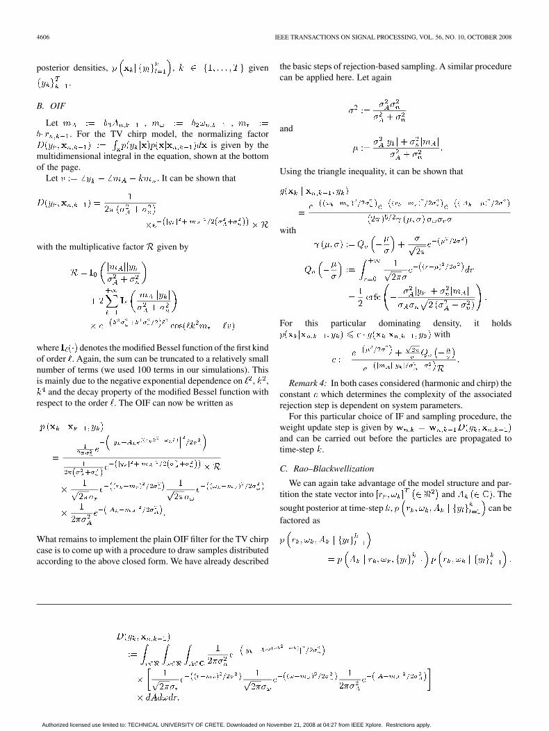
Let , ,. For the TV chirp model, the normalizing factor

is given by themultidimensional integral in the equation, shown at the bottomof the page.

Let . It can be shown that

with the multiplicative factor given by

where denotes the modified Bessel function of the first kindof order . Again, the sum can be truncated to a relatively smallnumber of terms (we used 100 terms in our simulations). Thisis mainly due to the negative exponential dependence on , ,

and the decay property of the modified Bessel function withrespect to the order . The OIF can now be written as

What remains to implement the plain OIF filter for the TV chirpcase is to come up with a procedure to draw samples distributedaccording to the above closed form. We have already described

the basic steps of rejection-based sampling. A similar procedurecan be applied here. Let again

and

Using the triangle inequality, it can be shown that

with

For this particular dominating density, it holdswith

Remark 4: In both cases considered (harmonic and chirp) theconstant which determines the complexity of the associatedrejection step is dependent on system parameters.

For this particular choice of IF and sampling procedure, theweight update step is given byand can be carried out before the particles are propagated totime-step .

C. Rao–Blackwellization

We can again take advantage of the model structure and par-tition the state vector into and . The

sought posterior at time-step , can befactored as



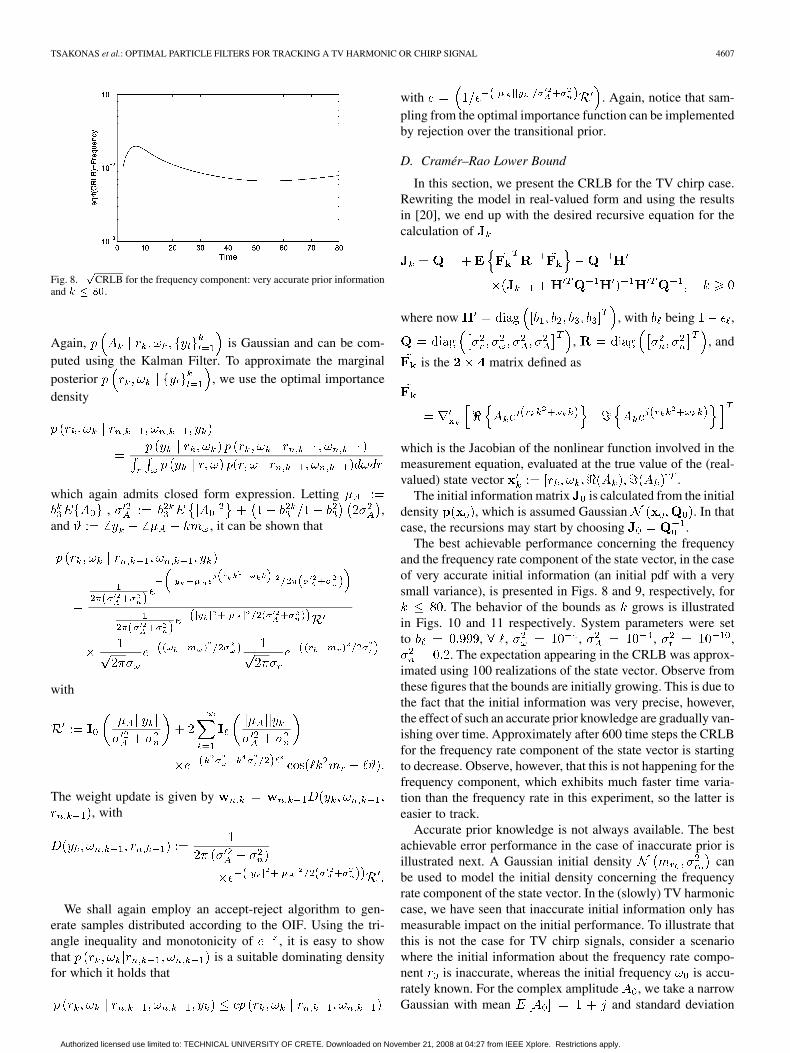
Fig. 8.�

CRLB for the frequency component: very accurate prior informationand � � ��.

Again, is Gaussian and can be com-puted using the Kalman Filter. To approximate the marginalposterior , we use the optimal importancedensity

which again admits closed form expression. Letting, ,

and , it can be shown that

with

The weight update is given by, with

We shall again employ an accept-reject algorithm to gen-erate samples distributed according to the OIF. Using the tri-angle inequality and monotonicity of , it is easy to showthat is a suitable dominating densityfor which it holds that

with . Again, notice that sam-pling from the optimal importance function can be implementedby rejection over the transitional prior.

D. Cramér–Rao Lower Bound

In this section, we present the CRLB for the TV chirp case.Rewriting the model in real-valued form and using the resultsin [20], we end up with the desired recursive equation for thecalculation of

where now , with being ,

, , and

is the matrix defined as

which is the Jacobian of the nonlinear function involved in themeasurement equation, evaluated at the true value of the (real-valued) state vector .

The initial information matrix is calculated from the initialdensity , which is assumed Gaussian . In thatcase, the recursions may start by choosing .

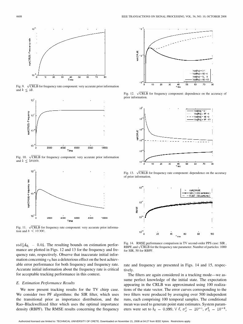
The best achievable performance concerning the frequencyand the frequency rate component of the state vector, in the caseof very accurate initial information (an initial pdf with a verysmall variance), is presented in Figs. 8 and 9, respectively, for

. The behavior of the bounds as grows is illustratedin Figs. 10 and 11 respectively. System parameters were setto , , , , ,

. The expectation appearing in the CRLB was approx-imated using 100 realizations of the state vector. Observe fromthese figures that the bounds are initially growing. This is due tothe fact that the initial information was very precise, however,the effect of such an accurate prior knowledge are gradually van-ishing over time. Approximately after 600 time steps the CRLBfor the frequency rate component of the state vector is startingto decrease. Observe, however, that this is not happening for thefrequency component, which exhibits much faster time varia-tion than the frequency rate in this experiment, so the latter iseasier to track.

Accurate prior knowledge is not always available. The bestachievable error performance in the case of inaccurate prior isillustrated next. A Gaussian initial density canbe used to model the initial density concerning the frequencyrate component of the state vector. In the (slowly) TV harmoniccase, we have seen that inaccurate initial information only hasmeasurable impact on the initial performance. To illustrate thatthis is not the case for TV chirp signals, consider a scenariowhere the initial information about the frequency rate compo-nent is inaccurate, whereas the initial frequency is accu-rately known. For the complex amplitude , we take a narrowGaussian with mean and standard deviation



Fig. 9.�

CRLB for frequency rate component: very accurate prior informationand � � ��.

Fig. 10.�

CRLB for frequency component: very accurate prior informationand � � ��.

Fig. 11.�

CRLB for frequency rate component: very accurate prior informa-tion and � � ��.

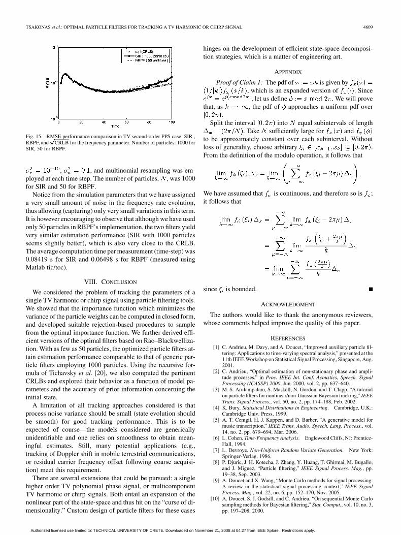
. The resulting bounds on estimation perfor-mance are plotted in Figs. 12 and 13 for the frequency and fre-quency rate, respectively. Observe that inaccurate initial infor-mation concerning has a deleterious effect on the best achiev-able error performance for both frequency and frequency rate.Accurate initial information about the frequency rate is criticalfor acceptable tracking performance in this context.

E. Estimation Performance Results

We now present tracking results for the TV chirp case.We consider two PF algorithms: the SIR filter, which usesthe transitional prior as importance distribution, and theRao–Blackwellized filter which uses the optimal importancedensity (RBPF). The RMSE results concerning the frequency

Fig. 12.�

CRLB for frequency component: dependence on the accuracy ofprior information.

Fig. 13.�

CRLB for frequency rate component: dependence on the accuracyof prior information.

Fig. 14. RMSE performance comparison in TV second-order PPS case: SIR ,RBPF, and

�CRLB for the frequency rate parameter. Number of particles: 1000

for SIR, 50 for RBPF.

rate and frequency are presented in Figs. 14 and 15, respec-tively.

The filters are again considered in a tracking mode—we as-sume perfect knowledge of the initial state. The expectationappearing in the CRLB was approximated using 100 realiza-tions of the state vector. The error curves corresponding to thetwo filters were produced by averaging over 500 independentruns, each comprising 100 temporal samples. The conditionalmean was used to generate point state estimates. System param-eters were set to , , , ,



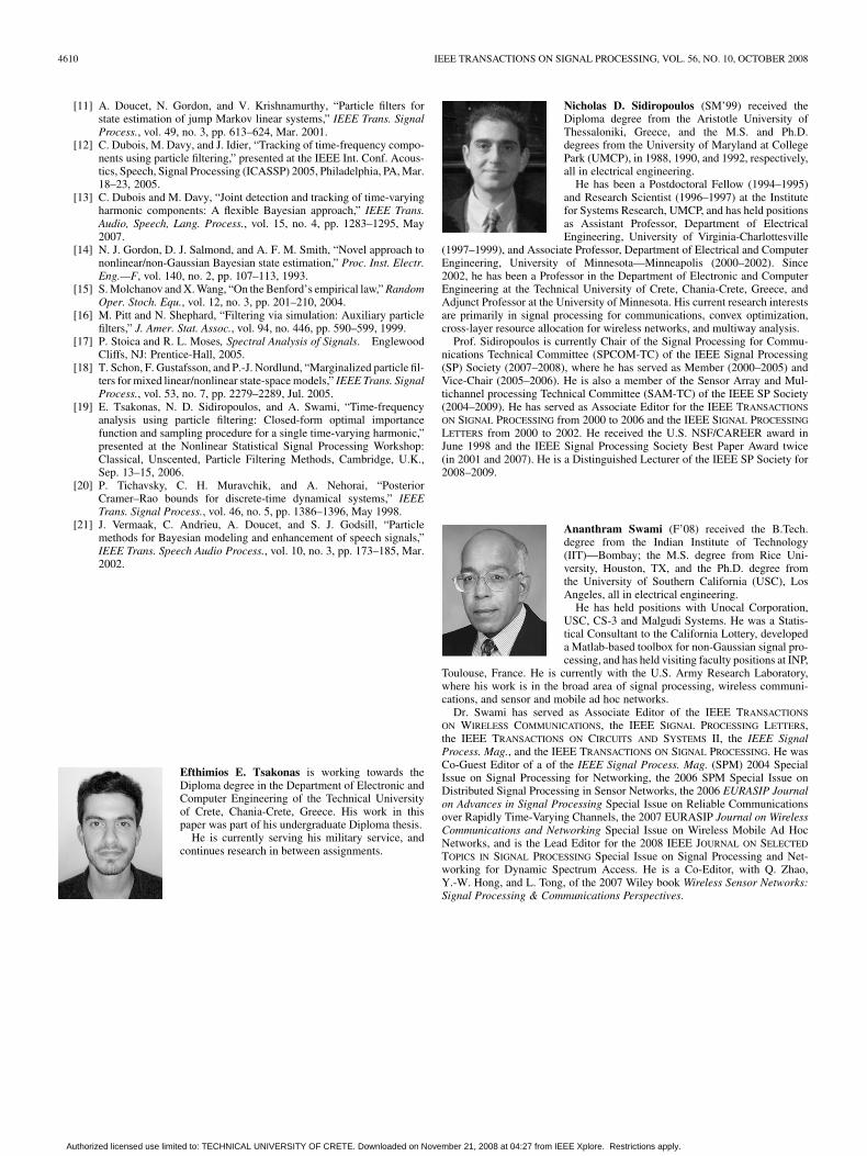
Fig. 15. RMSE performance comparison in TV second-order PPS case: SIR ,RBPF, and

�CRLB for the frequency parameter. Number of particles: 1000 for

SIR, 50 for RBPF.

, , and multinomial resampling was em-ployed at each time step. The number of particles, , was 1000for SIR and 50 for RBPF.

Notice from the simulation parameters that we have assigneda very small amount of noise in the frequency rate evolution,thus allowing (capturing) only very small variations in this term.It is however encouraging to observe that although we have usedonly 50 particles in RBPF’s implementation, the two filters yieldvery similar estimation performance (SIR with 1000 particlesseems slightly better), which is also very close to the CRLB.The average computation time per measurement (time-step) was0.08419 s for SIR and 0.06498 s for RBPF (measured usingMatlab tic/toc).

VIII. CONCLUSION

We considered the problem of tracking the parameters of asingle TV harmonic or chirp signal using particle filtering tools.We showed that the importance function which minimizes thevariance of the particle weights can be computed in closed form,and developed suitable rejection-based procedures to samplefrom the optimal importance function. We further derived effi-cient versions of the optimal filters based on Rao–Blackwelliza-tion. With as few as 50 particles, the optimized particle filters at-tain estimation performance comparable to that of generic par-ticle filters employing 1000 particles. Using the recursive for-mula of Tichavsky et al. [20], we also computed the pertinentCRLBs and explored their behavior as a function of model pa-rameters and the accuracy of prior information concerning theinitial state.

A limitation of all tracking approaches considered is thatprocess noise variance should be small (state evolution shouldbe smooth) for good tracking performance. This is to beexpected of course—the models considered are genericallyunidentifiable and one relies on smoothness to obtain mean-ingful estimates. Still, many potential applications (e.g.,tracking of Doppler shift in mobile terrestrial communications,or residual carrier frequency offset following coarse acquisi-tion) meet this requirement.

There are several extensions that could be pursued: a singlehigher order TV polynomial phase signal, or multicomponentTV harmonic or chirp signals. Both entail an expansion of thenonlinear part of the state-space and thus hit on the “curse of di-mensionality.” Custom design of particle filters for these cases

hinges on the development of efficient state-space decomposi-tion strategies, which is a matter of engineering art.

APPENDIX

Proof of Claim 1: The pdf of is given by, which is an expanded version of . Since

, let us define . We will provethat, as , the pdf of approaches a uniform pdf over

.Split the interval into equal subintervals of length

. Take sufficiently large for andto be approximately constant over each subinterval. Withoutloss of generality, choose arbitrary .From the definition of the modulo operation, it follows that

We have assumed that is continuous, and therefore so is ;it follows that

since is bounded.

ACKNOWLEDGMENT

The authors would like to thank the anonymous reviewers,whose comments helped improve the quality of this paper.

REFERENCES

[1] C. Andrieu, M. Davy, and A. Doucet, “Improved auxiliary particle fil-tering: Applications to time-varying spectral analysis,” presented at the11th IEEE Workshop on Statistical Signal Processing, Singapore, Aug.2001.

[2] C. Andrieu, “Optimal estimation of non-stationary phase and ampli-tude processes,” in Proc. IEEE Int. Conf. Acoustics, Speech, SignalProcessing (ICASSP) 2000, Jun. 2000, vol. 2, pp. 637–640.

[3] M. S. Arulampalam, S. Maskell, N. Gordon, and T. Clapp, “A tutorialon particle filters for nonlinear/non-Gaussian Bayesian tracking,” IEEETrans. Signal Process., vol. 50, no. 2, pp. 174–188, Feb. 2002.

[4] K. Bury, Statistical Distributions in Engineering. Cambridge, U.K.:Cambridge Univ. Press, 1999.

[5] A. T. Cemgil, H. J. Kappen, and D. Barber, “A generative model formusic transcription,” IEEE Trans. Audio, Speech, Lang. Process., vol.14, no. 2, pp. 679–694, Mar. 2006.

[6] L. Cohen, Time-Frequency Analysis. Englewood Cliffs, NJ: Prentice-Hall, 1994.

[7] L. Devroye, Non-Uniform Random Variate Generation. New York:Springer-Verlag, 1986.

[8] P. Djuric, J. H. Kotecha, J. Zhang, Y. Huang, T. Ghirmai, M. Bugallo,and J. Miguez, “Particle filtering,” IEEE Signal Process. Mag., pp.19–38, Sep. 2003.

[9] A. Doucet and X. Wang, “Monte Carlo methods for signal processing:A review in the statistical signal processing context,” IEEE SignalProcess. Mag., vol. 22, no. 6, pp. 152–170, Nov. 2005.

[10] A. Doucet, S. J. Godsill, and C. Andrieu, “On sequential Monte Carlosampling methods for Bayesian filtering,” Stat. Comput., vol. 10, no. 3,pp. 197–208, 2000.



[11] A. Doucet, N. Gordon, and V. Krishnamurthy, “Particle filters forstate estimation of jump Markov linear systems,” IEEE Trans. SignalProcess., vol. 49, no. 3, pp. 613–624, Mar. 2001.

[12] C. Dubois, M. Davy, and J. Idier, “Tracking of time-frequency compo-nents using particle filtering,” presented at the IEEE Int. Conf. Acous-tics, Speech, Signal Processing (ICASSP) 2005, Philadelphia, PA, Mar.18–23, 2005.

[13] C. Dubois and M. Davy, “Joint detection and tracking of time-varyingharmonic components: A flexible Bayesian approach,” IEEE Trans.Audio, Speech, Lang. Process., vol. 15, no. 4, pp. 1283–1295, May2007.

[14] N. J. Gordon, D. J. Salmond, and A. F. M. Smith, “Novel approach tononlinear/non-Gaussian Bayesian state estimation,” Proc. Inst. Electr.Eng.—F, vol. 140, no. 2, pp. 107–113, 1993.

[15] S. Molchanov and X. Wang, “On the Benford’s empirical law,” RandomOper. Stoch. Equ., vol. 12, no. 3, pp. 201–210, 2004.

[16] M. Pitt and N. Shephard, “Filtering via simulation: Auxiliary particlefilters,” J. Amer. Stat. Assoc., vol. 94, no. 446, pp. 590–599, 1999.

[17] P. Stoica and R. L. Moses, Spectral Analysis of Signals. EnglewoodCliffs, NJ: Prentice-Hall, 2005.

[18] T. Schon, F. Gustafsson, and P.-J. Nordlund, “Marginalized particle fil-ters for mixed linear/nonlinear state-space models,” IEEE Trans. SignalProcess., vol. 53, no. 7, pp. 2279–2289, Jul. 2005.

[19] E. Tsakonas, N. D. Sidiropoulos, and A. Swami, “Time-frequencyanalysis using particle filtering: Closed-form optimal importancefunction and sampling procedure for a single time-varying harmonic,”presented at the Nonlinear Statistical Signal Processing Workshop:Classical, Unscented, Particle Filtering Methods, Cambridge, U.K.,Sep. 13–15, 2006.

[20] P. Tichavsky, C. H. Muravchik, and A. Nehorai, “PosteriorCramer–Rao bounds for discrete-time dynamical systems,” IEEETrans. Signal Process., vol. 46, no. 5, pp. 1386–1396, May 1998.

[21] J. Vermaak, C. Andrieu, A. Doucet, and S. J. Godsill, “Particlemethods for Bayesian modeling and enhancement of speech signals,”IEEE Trans. Speech Audio Process., vol. 10, no. 3, pp. 173–185, Mar.2002.

Efthimios E. Tsakonas is working towards theDiploma degree in the Department of Electronic andComputer Engineering of the Technical Universityof Crete, Chania-Crete, Greece. His work in thispaper was part of his undergraduate Diploma thesis.

He is currently serving his military service, andcontinues research in between assignments.

Nicholas D. Sidiropoulos (SM’99) received theDiploma degree from the Aristotle University ofThessaloniki, Greece, and the M.S. and Ph.D.degrees from the University of Maryland at CollegePark (UMCP), in 1988, 1990, and 1992, respectively,all in electrical engineering.

He has been a Postdoctoral Fellow (1994–1995)and Research Scientist (1996–1997) at the Institutefor Systems Research, UMCP, and has held positionsas Assistant Professor, Department of ElectricalEngineering, University of Virginia-Charlottesville

(1997–1999), and Associate Professor, Department of Electrical and ComputerEngineering, University of Minnesota—Minneapolis (2000–2002). Since2002, he has been a Professor in the Department of Electronic and ComputerEngineering at the Technical University of Crete, Chania-Crete, Greece, andAdjunct Professor at the University of Minnesota. His current research interestsare primarily in signal processing for communications, convex optimization,cross-layer resource allocation for wireless networks, and multiway analysis.

Prof. Sidiropoulos is currently Chair of the Signal Processing for Commu-nications Technical Committee (SPCOM-TC) of the IEEE Signal Processing(SP) Society (2007–2008), where he has served as Member (2000–2005) andVice-Chair (2005–2006). He is also a member of the Sensor Array and Mul-tichannel processing Technical Committee (SAM-TC) of the IEEE SP Society(2004–2009). He has served as Associate Editor for the IEEE TRANSACTIONS

ON SIGNAL PROCESSING from 2000 to 2006 and the IEEE SIGNAL PROCESSING

LETTERS from 2000 to 2002. He received the U.S. NSF/CAREER award inJune 1998 and the IEEE Signal Processing Society Best Paper Award twice(in 2001 and 2007). He is a Distinguished Lecturer of the IEEE SP Society for2008–2009.

Ananthram Swami (F’08) received the B.Tech.degree from the Indian Institute of Technology(IIT)—Bombay; the M.S. degree from Rice Uni-versity, Houston, TX, and the Ph.D. degree fromthe University of Southern California (USC), LosAngeles, all in electrical engineering.

He has held positions with Unocal Corporation,USC, CS-3 and Malgudi Systems. He was a Statis-tical Consultant to the California Lottery, developeda Matlab-based toolbox for non-Gaussian signal pro-cessing, and has held visiting faculty positions at INP,

Toulouse, France. He is currently with the U.S. Army Research Laboratory,where his work is in the broad area of signal processing, wireless communi-cations, and sensor and mobile ad hoc networks.

Dr. Swami has served as Associate Editor of the IEEE TRANSACTIONS

ON WIRELESS COMMUNICATIONS, the IEEE SIGNAL PROCESSING LETTERS,the IEEE TRANSACTIONS ON CIRCUITS AND SYSTEMS II, the IEEE SignalProcess. Mag., and the IEEE TRANSACTIONS ON SIGNAL PROCESSING. He wasCo-Guest Editor of a of the IEEE Signal Process. Mag. (SPM) 2004 SpecialIssue on Signal Processing for Networking, the 2006 SPM Special Issue onDistributed Signal Processing in Sensor Networks, the 2006 EURASIP Journalon Advances in Signal Processing Special Issue on Reliable Communicationsover Rapidly Time-Varying Channels, the 2007 EURASIP Journal on WirelessCommunications and Networking Special Issue on Wireless Mobile Ad HocNetworks, and is the Lead Editor for the 2008 IEEE JOURNAL ON SELECTED

TOPICS IN SIGNAL PROCESSING Special Issue on Signal Processing and Net-working for Dynamic Spectrum Access. He is a Co-Editor, with Q. Zhao,Y.-W. Hong, and L. Tong, of the 2007 Wiley book Wireless Sensor Networks:Signal Processing & Communications Perspectives.


optimal particle filters for tracking a time-varying harmonic or

Documents