FEDERAL RESERVE BANK OF SAN FRANCISCO

WORKING PAPER SERIES

Optimal Policy in Rational Expectations Models: New Solution Algorithms

Richard Dennis Federal Reserve Bank of San Francisco

September 2005

Working Paper 2001-09 http://www.frbsf.org/publications/economics/papers/2001/wp01-09bk.pdf

The views in this paper are solely the responsibility of the authors and should not be interpreted as reflecting the views of the Federal Reserve Bank of San Francisco or the Board of Governors of the Federal Reserve System.

Optimal Policy in Rational Expectations Models:

New Solution Algorithms∗

Richard Dennis†

Federal Reserve Bank of San Francisco

September 2005

Abstract

This paper develops methods to solve for optimal discretionary policies and optimalcommitment policies in rational expectations models. These algorithms, which allowthe optimization constraints to be conveniently expressed in second-order structural form,are more general than existing methods and are simple to apply. We use several NewKeynesian business cycle models to illustrate their application. Simulations show that theprocedures developed in this paper can quickly solve small-scale models and that they canbe usefully and effectively applied to medium- and large-scale models.

1 INTRODUCTION

Central banks and other policymakers are commonly modeled as agents whose objective is

to minimize some loss function subject to constraints that contain forward-looking rational

expectations (see Woodford (2002), Clarida, Galí, and Gertler, (1999), or the Taylor (1999)

conference volume, for example). But of course Kydland and Prescott (1977) showed that

in the absence of some commitment mechanism optimal policies were time-inconsistent. The

modern policy literature addresses this time-consistency problem either by simply assuming

that the policymaker can commit to not reoptimize or by explicitly modeling the strategic

interactions that occur between the various economic agents in the model.1 When the former

approach is taken the policymaker commits to undertake a single optimization and implements

∗I would like to thank the associate editor and two anonymous referees for comments. I would also like tothank Kirk Moore for research assistance. The views expressed in this paper do not necessarily reflect thoseof the Federal Reserve Bank of San Francisco or the Federal Reserve System.

†Address for correspondence: Economic Research, Mail Stop 1130, Federal Reserve Bank of San Francisco,101 Market St, CA 94105, USA. Email: richard.dennis@sf.frb.org.

1 An alternative approach is to assume that the policymaker sets policy according to a “timeless perspective”(Woodford, 1999). According to the timelsss perspective the policymaker optimizing today behaves as it wouldhave chosen to if it had optimized at a time far in the past. Useful discussions and analyses of timelesslyoptimal policies can be found in Giannoni and Woodford (2002) and Jensen and McCallum (2002).

1

the chosen policy in all subsequent periods. When the latter approach is pursued the technique

is to solve for a subgame-perfect equilibrium. While other time-consistent equilibria could be

studied,2 it is most common to solve for Markov-perfect Stackelberg-Nash equilibria in which

the policymaker is the Stackelberg leader and private-sector agents and future policymakers

are Stackelberg followers.

Several methods for solving for optimal commitment policies and for Markov-perfect Stackelberg-

Nash equilibria (optimal discretionary policies in what follows) have been developed. For com-

mitment, available algorithms include those developed in Currie and Levine (1985, 1993) and

Söderlind (1999), which are based on Hamiltonian and Lagrangian methods, respectively, and

Backus and Driffill (1986), which transforms the solution to a dynamic programming problem

to obtain the commitment policy. For discretion, two popular algorithms are those developed

by Oudiz and Sachs (1985) and Backus and Driffill (1986). Both Oudiz and Sachs (1985)

and Backus and Driffill (1986) solve for optimal discretionary rules using dynamic program-

ming, but Oudiz and Sachs (1985) solve for the stationary feedback rule by taking the limit

as t → −∞ of a finite horizon problem while Backus and Driffill (1986) solve the asymptotic

problem directly.3 By construction optimal discretionary policies are time-consistent.

A feature common to all of these solution methods is that they require the optimization

constraints to be written in state-space form. An attractive feature of the state-space form

is that it provides a compact and efficient representation of an economic model in a form

that contains only first-order dynamics. However, reliance on the state-space form also has

disadvantages. In particular, use of the state-space representation forces the distinction

between predetermined and non-predetermined variables and often requires considerable effort

to manipulate the model in the required form. Both of these requirements, but especially the

latter, mean that these solution methods come with “overhead” costs that can be considerable.

In this paper we develop algorithms to solve for optimal commitment policies and optimal

discretionary policies that differ from existing algorithms in that they allow the constraints

to be written in structural form rather than in state-space form. As a broadbrush char-

acterization, for small-scale models that have only a few non-predetermined variables, it is

generally not too difficult to express the model in state-space form, in which case solving the

model using a state-space solution method may be convenient. However, even for models

2 See Holly and Hughes-Hallett (1989), Amman and Kendrick (1999), Chen and Zadrozney (2002), and Blake(2004), for other approaches.

3 Söderlind (1999) provides a popular implementation of the Backus and Driffill (1986) algorithm. Krusell,Quadrini, and Rios-Rull (1997) provide an alternative, guess-and-verify, approach to solving for time-consistentpolicies.

2

that are only modestly complex it is often much easier to write the model in structural form,

and the algorithms presented here have been developed with these models in mind.4 While

of interest in their own right, the algorithms developed here also have several other useful

attributes. First, they do not require the predetermined variables to be separated from the

non-predetermined variables; second, they can be easily applied to models whose optimiza-

tion constraints contain the expectation of next period’s policy instrument(s); and third, they

supply the Euler equation for the optimal discretionary policy, which makes them particularly

convenient when a “targeting rule” rather than an “instrument rule” (see Svensson, 2003) is

sought.

Although the relative strength of these algorithms is that they can be easily applied to

models that are difficult to manipulate into a state-space form, to illustrate their use we apply

them to several, reasonably simple, New Keynesian models and compare their properties to

existing solution methods. For this comparison, we take the models developed by Galí and

Monacelli (2005) and Erceg, Henderson, and Levin (2000) and solve for optimal commitment

policies and optimal discretionary policies for a range of policy regimes. Although the al-

gorithms developed in this paper exploit less model structure than the state-space methods,

they are still reasonably efficient. To demonstrate that they can usefully solve larger models,

we also apply them to the model developed by Fuhrer and Moore (1995).5

The remainder of this paper is structured as follows. The following section introduces

the components of the policymaker’s optimization problem, describing the objective function

and the equations that constrain the optimization process. Section 3 shows how to solve

for optimal commitment rules. Section 4 turns to discretion. The discretionary problem is

formulated in terms of an unconstrained optimization, which contrasts with the more usual

dynamic programming or Lagrangian-based approaches. In section 5 we employ two New

Keynesian models to calculate the computation times of a range of solution methods. Section

5 also discusses situations for which convergence problems can be encountered when solving

for optimal policies. Section 6 concludes while appendices contain technical details.

4 Dennis (2004a) shows how to solve for optimal simple rules when the optimization constraints are writtenin structural form.

5 Dennis and Söderström (2005) apply the methods developed in this paper to the macro-policy modeldeveloped by Orphanides and Wieland (1998), which is somewhat more complicated than the Fuhrer andMoore (1995) model.

3

2 THE OPTIMIZATION PROBLEM

Let yt be an (n×1) vector of endogenous variables and xt be a (p×1) vector of policy instru-

ments. For convenience, the variables in yt and xt represent deviations from nonstochastic

steady-state values. The policymaker sets xt to minimize the loss function6

Loss (t0,∞) = Et0

∞∑

t=0

βt[y′tWyt + x

′tQxt

], (1)

where β ∈ (0, 1) is the discount factor and W (n× n) and Q (p× p) are symmetric, positive

semi-definite, matrices containing policy preferences, or policy tastes. Here Et0 represents the

mathematical expectations operator conditional upon period t0 information. Loss functions

like (1) are widely employed in the literature because, with linear constraints, they lead to

linear decision rules. Furthermore, as is now well documented, this loss function can represent

a second-order approximation to a representative agent’s utility function (see Diaz-Gimenez,

1999, for example) and in certain situations it collapses to an expression containing just output

and inflation (Woodford, 2002).

The policymaker minimizes (1) subject to the following system of dynamic constraints7

A0yt = A1yt−1 +A2Etyt+1 +A3xt +A4Etxt+1 +A5vt, (2)

where vt ∼ iid [0,Ω] is an (s× 1, s ≤ n) vector of innovations and the matrices A0, A1, A2,

A3, A4, and A5 contain the model’s structural parameters, which are conformable with yt,

xt, and vt, as necessary. The dating convention in (2) is such that every element in yt−1 has

a known value as of the beginning of period t. A0 is assumed to be non-singular.

It is not necessary to explicitly include the matrix A5 in (2) because it is always possible

to include vt within yt. However, its presence allows us to easily accommodate models where

the innovations are scaled by structural parameters without having to expand the state vector

or redefine the innovations. An important feature of (2) is that it contains not just the

contemporaneous policy instruments, but also the expectation of next period’s instrument

vector, which is useful for models that contain an interest rate term structure, for example.8

6 The omission of terms interacting yt and xt in equation (1) is without loss of generality. When theconstraints are in structural form it is always possible in include xt within yt with W containing the relevantpenalty terms.

7 Binder and Pesaran (1995) show how a wide class of models, which can contain quite general lead-lagstructures and expectations formed with varying information sets, can be written in terms of (2).

8 Svensson (2000) also solves a model that contains the expected future value of the policy instrument.However, Svensson (2000) considers discretion, but not commitment.

4

3 Commitment

Under commitment the policymaker optimizes once and never reoptimizes. The assumption

is that either the policymaker can adhere to its chosen policy or that the discount factor is

sufficiently large to allow the chosen policy to be supported as a reputation equilibrium (see

Currie and Levine, 1993, chapter 5). To solve for optimal commitment policies, we observe

that from the definition of rational expectations we can write

yt+1 = Etyt+1 + ηt+1 (3)

xt+1 = Etxt+1 +µt+1, (4)

where the expectation errors, ηt+1 and µt+1, are martingale difference sequences. Substituting

(3) and (4) into (2) gives

A0yt = A1yt−1 +A2yt+1 +A3xt +A4xt+1 + ρt (5)

ρt = A5vt −A2ηt+1 −A4µt+1. (6)

To solve the optimization problem from the standpoint of period t0 we form the Lagrangian

L = Et0

∞∑

t=t0

β(t−t0) [y′tWyt + x′tQxt (7)

+2λ′t (A0yt −A1yt−1 −A2yt+1 −A3xt −A4xt+1 − ρt)]

and take derivatives with respect to xt, yt, and λt, giving9

∂L

∂xt= Qxt −A

′3λt − β−1A′4λt−1 = 0, t > t0 (8)

∂L

∂yt= Wyt +A

′0λt − β−1A′2λt−1 − βA′1Etλt+1 = 0, t > t0 (9)

∂L

∂λt= A0yt −A1yt−1 −A2Etyt+1 −A3xt −A4Etxt+1 −A5vt = 0, t ≥ t0 (10)

∂L

∂xt= Qxt −A

′3λt = 0, t = t0 (11)

∂L

∂yt= Wyt +A

′0λt − βA′1Etλt+1 = 0, t = t0, (12)

where yt0−1 = y. The fact that the policymaker behaves differently in the first period than it

does in subsequent periods in reflected in the fact that (11) and (12) apply in the initial period

(t = t0) whereas (8) and (9) apply in all subsequent periods. However, the recursive nature of

9 Because W and Q are symmetric positive semi-definite and the policy constraints are convex the Lagrangianis also convex and the first-order conditions are sufficient for locating the minimum.

5

the system can be restored by employing (8) - (10), for all t ≥ t0, but with the initial conditions

yt0−1 = y and λt0−1 = 0.10 The Lagrange multipliers equal zero at the start of the initial

period because, as implied by (11) and (12), the policymaker exploits agent’s expectations

in the initial period, while promising never to do so in the future (Kydland and Prescott,

1980). It is worth noting that it is the very fact that the policymaker behaves differently in

the initial period that provides the starting values for the Lagrange multipliers that are needed

for the first-order conditions to have a unique, stable, rational expectations equilibrium. The

presence of the expected future instrument vector in the optimization constraints presents no

special difficulties because the policymaker optimizes only once and the dynamics arising from

this term can easily be accounted for during that optimization.

Given yt0−1 = y and λt0−1 = 0, (8) — (10), can be solved in a number of ways. One

possibility is to write them in second-order form

0 A0 −A3A′0 W 0

−A′3 0 Q

λtytxt

=

0 A1 0

β−1A′2 0 0

β−1A′4 0 0

λt−1yt−1xt−1

(13)

+

0 A2 A4βA′1 0 0

0 0 0

Et

λt+1yt+1xt+1

+

A50

0

[vt] (14)

and to apply an undetermined-coefficient technique, such as these developed by Binder and

Pesaran (1995), McCallum (1999), or Uhlig (1999). An alternative approach is to write (8) —

(10) in first-order form

MΓt =NEtΓt+1 +Υt, (15)

where

M =

0 −A1 0 A0 −A3−β−1A′2 0 A′0 W 0

0 0 I 0 0

0 0 0 I 0

−β−1A′4 0 −A′3 0 Q

,Γt =

λt−1yt−1λtytxt

,

N =

0 0 0 A2 A40 0 βA′1 0 0

I 0 0 0 0

0 I 0 0 0

0 0 0 0 0

,Υt =

A50

0

0

0

[vt]

10 More precisely, the constraints on λt0−1 are

[A

′

2

A′

4

]λt0−1 = 0. Because dim

[ker

([A

′

2

A′

4

])]is not

necessarily zero, the restriction in the text, λt0−1 = 0, is sufficient, but stronger than necessary.

6

and to solve the system using an eigenvalue method, such as Anderson and Moore (1985),

Klein (2000), King and Watson (2002), Christiano (2002), or Sims (2002). Notice that the

vectors in (15) have been allocated such that the predetermined variables, λt−1 and yt−1, enter

at the top of the system, the “stable” block, while the jump variables, λt, yt, and xt, enter at

the bottom, the “unstable” block. The order of the variables within these vectors is irrelevant

since by construction every element in λt−1 and yt−1 has a known value at the beginning of

period t. While the order of the variables within the system is an issue for many solution

methods, here one simply orders vectors, which makes these Euler equations particularly easy

to solve.

Both undetermined-coefficient methods and eigenvalue methods return solutions in the

form λtytxt

=

θ11 θ12 0

θ21 θ22 0

ϕ1 ϕ2 0

λt−1yt−1xt−1

+

θ13θ23ϕ3

[ vt

]. (16)

The optimal commitment rule can be seen in (16) to depend on the vector of lagged Lagrange

multipliers. These Lagrange multipliers enter the rule to ensure that today’s policy validates

how private sector expectations were formed in the past.

Remark 1: The Euler equations for optimal commitment policy, (8) — (10), do not depend

on the covariance matrix of the shocks, Ω. Consequently, optimal commitment policies

are certainty equivalent.

Remark 2: Let zt ≡[λ′t y′t x′t

]′, K ≡

0 0 0

0 W 0

0 0 Q

, and, in obvious notation, (16) be

written as zt = Hzt−1 +Gvt. Then, the loss function can be written as Loss (t,∞) =[z′t−1H

′PHzt−1 + v

′

tG′PGvt +

β

1− βtr(G′PGΩ

)], where P ≡ K+βH′PH (see Ap-

pendix A2).

Remark 3: A consequence of Remark 2 is that limβ↑1(1− β)Loss (t,∞) = tr (KΦ) where Φ

is the unconditional variance-covariance matrix of[y′

t x′

t

]′and K ≡

[W 0

0 Q

](see

Appendix A3).

4 Discretion

In this section we consider discretion and develop a numerical procedure that solves for Markov-

perfect Stackelberg-Nash equilibria in which the policymaker optimizing today is the Stack-

7

elberg leader and private sector agents and future policymakers are Stackelberg followers.

Broadly, the innovations in this section are that we allow expected future instruments to enter

the optimization constraints and that we base the algorithm on a framework in which the

optimization constraints are written in structural form, not in state-space form. The outcome

is a solution procedure that is easy to apply and that eliminates the need to represent the

optimization constraints in state-space form. The solution method also returns the Euler

equations associated with the optimal discretionary policy, not just the decisions rules, which

makes it particularly well suited for studying “targeting rules” (Svensson, 2003).

Because the system’s state variables are yt−1 and vt, in the equilibrium that we seek

the endogenous variables and the policy instruments will all be functions of these variables.

Assume, then, that a stationary solution to the policymaker’s optimization problem exists and

is given by

yt = H1yt−1 +H2vt (17)

xt = F1yt−1 +F2vt. (18)

It is the time-invariant matrices H1, H2, F1, and F2 that we seek.

Substituting (17) and (18) into (2) gives

Dyt = A1yt−1 +A3xt +A5vt (19)

where

D ≡ A0 −A2H1 −A4F1. (20)

The matrix D embeds how future policymakers respond to movements in yt and the policy-

maker setting xt today allows for D, rather than just A0, when calculating the impact of its

policy decisions. Thus, future policymakers are followers with respect to current policymakers.

Using (17) and (18), we can express the loss function in terms of H1, H2, F1, F2, yt and

the instrument vector, xt as (see Appendix B1)

Loss (t,∞) = y′tPyt + x′tQxt +

β

1− βtr[(F′2QF2 +H

′2PH2

)Ω]

(21)

where

P ≡W+ βF′1QF1 + βH′1PH1. (22)

While a Lagrangian could be used, it is just as simple to substitute (19) into (21) and transform

what was a constrained optimization problem into an unconstrained optimization problem.

8

Following this substitution we have11

Loss (t,∞) = (A1yt−1 +A3xt +A5vt)′

D′−1PD−1 (A1yt−1 +A3xt +A5vt)

+x′tQxt +β

1− βtr[(F′2QF2 +H

′2PH2

)Ω]. (23)

Differentiating (23) with respect to xt and setting the resulting derivative equal to zero gives

∂Loss (t,∞)

∂xt= A′3D

′−1PD−1 (A1yt−1 +A5vt) +(Q+A′3D

′−1PD−1A3)xt = 0. (24)

Equation (24) can alternatively be expressed in terms of endogenous variables as

Qxt +A′3D

′−1Pyt = 0, (25)

which is useful when a “targeting rule” rather than an “instrument rule” (Svensson, 2003) is

of interest. Solving (24) for xt produces

xt = −(Q+A′3D

′−1PD−1A3)−1

A′3D′−1PD−1 (A1yt−1 +A5vt)

≡ F1yt−1 +F2vt, (26)

which when inserted back into (19) leads to

yt = D−1 (A1 +A3F1)yt−1 +D−1 (A5 +A3F2)vt

≡ H1yt−1 +H2vt. (27)

Of course both P and D are implicit functions of H1, H2, F1, and F2. Thus (26) and (27)

must be solved for a fixed point to obtain the desired solution. The numerical procedure is

as follows

Step 1) Initialize H1, H2, F1, and F2.

Step 2) Solve for D according to (20) and for P from (22), iterating “backward through

time” using a method such as the doubling algorithm.12

Step 3) Update H1, H2, F1, and F2 according to

F1 = −(Q+A′3D

′−1PD−1A3)−1

A′3D′−1PD−1A1, (28)

F2 = −(Q+A′3D

′−1PD−1A3)−1

A′3D′−1PD−1A5, (29)

H1 = D−1 (A1 +A3F1) , (30)

H2 = D−1 (A5 +A3F2) . (31)

11 This transformation requires that D have full rank, which is invariably satisfied because A0 has full rank.12 A description of the doubling algorithm along with other methods for solving matrix Sylvester equations

can be found in Anderson, Hansen, McGrattan, and Sargent (1996).

9

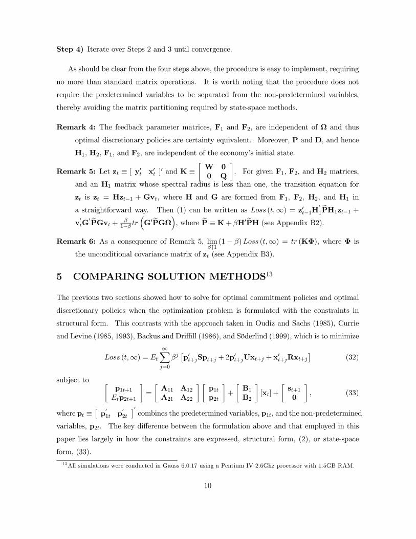
Step 4) Iterate over Steps 2 and 3 until convergence.

As should be clear from the four steps above, the procedure is easy to implement, requiring

no more than standard matrix operations. It is worth noting that the procedure does not

require the predetermined variables to be separated from the non-predetermined variables,

thereby avoiding the matrix partitioning required by state-space methods.

Remark 4: The feedback parameter matrices, F1 and F2, are independent of Ω and thus

optimal discretionary policies are certainty equivalent. Moreover, P and D, and hence

H1, H2, F1, and F2, are independent of the economy’s initial state.

Remark 5: Let zt ≡ [ y′t x′t ]

′ and K ≡

[W 0

0 Q

]. For given F1, F2, and H2 matrices,

and an H1 matrix whose spectral radius is less than one, the transition equation for

zt is zt = Hzt−1 + Gvt, where H and G are formed from F1, F2, H2, and H1 in

a straightforward way. Then (1) can be written as Loss (t,∞) = z′t−1H′

1PH1zt−1 +

v′

tG′PGvt +

β1−β tr

(G′PGΩ

), where P ≡K+ βH′PH (see Appendix B2).

Remark 6: As a consequence of Remark 5, limβ↑1(1− β)Loss (t,∞) = tr (KΦ), where Φ is

the unconditional covariance matrix of zt (see Appendix B3).

5 COMPARING SOLUTION METHODS13

The previous two sections showed how to solve for optimal commitment policies and optimal

discretionary policies when the optimization problem is formulated with the constraints in

structural form. This contrasts with the approach taken in Oudiz and Sachs (1985), Currie

and Levine (1985, 1993), Backus and Driffill (1986), and Söderlind (1999), which is to minimize

Loss (t,∞) = Et

∞∑

j=0

βj[p′t+jSpt+j + 2p

′t+jUxt+j + x

′t+jRxt+j

](32)

subject to [p1t+1

Etp2t+1

]=

[A11 A12A21 A22

][p1tp2t

]+

[B1B2

][xt] +

[st+10

], (33)

where pt ≡[p′

1t p′

2t

]′combines the predetermined variables, p1t, and the non-predetermined

variables, p2t. The key difference between the formulation above and that employed in this

paper lies largely in how the constraints are expressed, structural form, (2), or state-space

form, (33).

13 All simulations were conducted in Gauss 6.0.17 using a Pentium IV 2.6Ghz processor with 1.5GB RAM.

10

In this section we apply the algorithms developed in sections 3 and 4 to two optimization-

based New Keynesian models and compare their computation times to state-space solution

methods. Because optimal commitment policies and optimal discretionary policies are often

studied in the monetary policy literature, the models that we analyze are drawn from that

literature. We study the small open-economy model developed by Galí and Monacelli (2005)

and closed-economy model developed by Erceg, Henderson, and Levin (2000) (EHL), both

are representative of the models used to examine monetary policy issues. For discretion, we

compare the algorithm developed in section 4 to those developed in Oudiz and Sachs (1985) and

Backus and Driffill (1986). For commitment, we compare the algorithm presented in section

3 to those developed by Backus and Driffill (1986) and Söderlind (1999). Subsequently, we

apply our procedures to the larger Fuhrer and Moore (1995) model and discuss situations

where convergence problems can sometimes be encountered when solving for optimal policies.

Solving for optimal commitment policies using the approach of section 3 requires solv-

ing a rational expectations (RE) model and there are numerous techniques available to per-

form this task. We take the opportunity to compare two RE solution methods, the “brute

force” undetermined-coefficient method presented in Binder and Pesaran (1995) and the QZ-

decomposition method presented in Klein (2000). For the latter, we used both the real QZ

decomposition and the complex QZ decomposition,14 however only the computation times for

the real QZ decomposition are reported since they were uniformly faster than those for the

complex QZ decomposition.15

5.1 A small-scale open-economy model

In the open-economy model developed by Galí and Monacelli (2005), households consume

an aggregate of domestically produced and imported goods. The law-of-one-price applies to

imported goods. Domestic firms are monopolistically competitive and subject to Calvo-style

price rigidities (Calvo, 1983). Financial assets are internationally tradable and nominal un-

covered interest parity holds. The law-of-one-price together with the definition for consumer

price inflation implies that the real exchange rate and the terms-of-trade are perfectly corre-

lated, while nominal uncovered interest parity coupled with the law-of-one-price implies that

real uncovered interest parity holds.

14 Routines to perform the real QZ decomposition and the complex QZ decomposition in Gauss are availablefrom Paul Söderlind’s website. These excellent routines were employed in this study.

15 Söderlind’s (1999) method of solving for commitment equilibria also utilizes the real QZ decomposition.

11

For our purposes, the relevant model equations are16

yt = Etyt+1 −ωα

σ(it −Etπt+1) + gt

πt = βEtπt+1 + καyt + ut

πct = πt +α

1− α(qt − qt−1)

qt = Etqt+1 − (1− α)(it −Etπt+1 − i∗t +Etπ

∗t+1

)+ (1− α) ǫt,

where yt denotes the output gap, πt denotes domestic goods’ inflation, πct denotes consumer

price inflation rate, qt denotes the real exchange rate (an increase in qt represents a real

depreciation), it and i∗t denote domestic and foreign nominal interest rates, respectively, π∗t

denotes foreign inflation, and gt, ut, and ǫt are white noise shocks.17

The central bank sets the nominal interest rate, it, to minimize the loss function

Loss(t,∞) = Et

∞∑

j=0

βj[(πct+j

)2+ λy2t+j + ν (it+j − it+j−1)

2], (34)

where the policy preference parameters, λ and ν, are restricted to be non-negative. In the

experiments that follow, we consider a range of policy preference parameters, allowing λ to

take on the values 0, 1, and 3 and ν to take on the values 0, 12 and 1.

5.1.1 Solution times

We first assume that policy is set with discretion. Table 1 reports the time it takes to solve

the Galí-Monacelli model using the algorithm in section 4 and the algorithms in Oudiz and

Sachs (1985), Backus and Driffill (1986), and Söderlind (1999).18 The procedure presented in

Söderlind (1999) is the same as Backus and Driffill (1986) and for this reason both algorithms

are attributed the same computation time.

16 The structural form and the state-space form used for the Galí-Monacelli model are contained in a technicalappendix that is available upon request.

17 We follow Galí and Monacelli (2004) and set η = 1, α = 0.4, β = 0.99, θ = 0.75, σ = 1, ϕ = 3,

ωα = 1 + α (2− α) (ση − 1) , and κα = (1−θ)(1−βθ)θ

(ϕ+ σ

ωα

). We condition on the foreign variables and

normalize their values to zero.18 The model was solved 100,000 times using each algorithm from which average solution times were computed.

The convergence criteria were set so that the algorithms all returned solutions that were identical to thirteensignificant figures.

12

Table 1: Solution Times under Discretion(hundreds of seconds)

Section 4 Oudiz-Sachs Backus-Driffill/Regime Söderlind

(λ, ν) = (0, 0) 0.09 0.16 0.16(λ, ν) =

(0, 12

)0.17 0.16 0.17

(λ, ν) = (0, 1) 0.19 0.17 0.18(λ, ν) = (1, 0) 0.15 0.11 0.11(λ, ν) =

(1, 12

)0.14 0.12 0.12

(λ, ν) = (1, 1) 0.16 0.12 0.12(λ, ν) = (3, 0) 0.08 0.08 0.08(λ, ν) =

(3, 12

)0.12 0.09 0.10

(λ, ν) = (3, 1) 0.12 0.10 0.10

The first point to note is that all of the algorithms are able to quickly obtain the optimal

discretionary rule for each parameter combination considered. At the same time, the results

indicate that the Oudiz-Sachs algorithm is the fastest for this model, but only marginally;

the difference between the fastest algorithm (Oudiz-Sachs) and the slowest algorithm (section

4) is just 0.00012 second on average. It takes slightly longer to solve the model when the

constraints are in structural form because the structural form does not exploit as much of the

model’s structure as the state-space form does. No convergence problems were encountered

with any of the algorithms.

Table 2: Solution Times under Commitment(hundreds of seconds)

Section 3 Backus-Driffill Söderlind

Regime Binder-Pesaran Real-QZ Dyn. Prog. Real-QZ

(λ, ν) = (0, 0) — — — —(λ, ν) =

(0, 12

)0.10 0.13 0.07 0.09

(λ, ν) = (0, 1) 0.12 0.12 0.09 0.09(λ, ν) = (1, 0) 0.15 0.11 — 0.05(λ, ν) =

(1, 12

)0.21 0.12 0.14 0.08

(λ, ν) = (1, 1) 0.19 0.12 0.14 0.09(λ, ν) = (3, 0) 0.27 0.11 — 0.05(λ, ν) =

(3, 12

)0.29 0.12 0.21 0.08

(λ, ν) = (3, 1) 0.30 0.12 0.21 0.08

Turning to the commitment solution methods, Table 2 shows that for the algorithms that

use recursive methods — Binder-Pesaran and Backus-Driffill — the solution time is increasing in

λ and ν. The algorithms that obtain the commitment policy using the real QZ decomposition

are both quicker in general that the recursive methods and have solution times that are largely

invariant to the loss function’s parameterization. As with discretion, use of the structural

13

form weighs on the computation time slightly. Table 2 also shows that for this model the

Backus-Driffill algorithm cannot obtain the solution when ν = 0, regardless of the value for

λ.19 In fact, none of the algorithms are able to obtain a solution when λ = ν = 0. For the

Binder-Pesaran method the matrix recursion used to solve the RE model does not converge,

although the iterations do converge when ν is small, but non-zero. The procedures that rely

on eigenvalue methods determine the correct number of unstable eigenvalues, but a singularity

prevents the jump variables from being related to the predetermined variables in a way that

eliminates the unstable dynamics.20 The fact that the problem occurs regardless of whether

the model is in structural or state-space form shows that it is not idiosyncratic to one particular

formulation of the optimization problem.

5.2 A small-scale closed-economy model

The second model that we examine is that developed by Erceg, Henderson, and Levin (2000)

(EHL). EHL assume that both prices and wages are subject to Calvo-contracts, but the

model is otherwise a standard New Keynesian business cycle model with monopolistically

competitive firms. When log-linearized about the model’s Pareto optimal equilibrium, the

relevant equations are21

gt = Etgt+1 −1

σlc(it −Etπt+1 − r∗t )

πt = βEtπt+1 + κρ (wt −mplt)

wt = βEtwt+1 + κρ (mrst −wt)

mplt = w∗t − λmplgt

mrst = w∗t + λmrsgt

wt = wt−1 +wt − πt

r∗t = σlc(Ety

∗t+1 − y∗t

)+ σlq (Etqt+1 − qt)

w∗t = w∗xxt +w∗qqt +w∗zzt

y∗t = y∗xxt + y∗qqt + y∗zzt

xt = ρxt−1 + επt,

19 The source of this difficulty is a singularity in the transformation the algorithm uses to rotate the dynamicprogramming solution into state/co-state space.

20 This instability differs from the standard form of instability encountered in rational expectations models,which is that the system contains more unstable eigenvalues than there are non-predetermined variables.

21 The structural form and the state-space form used for the EHL model are contained in a technical appendixthat is available upon request.

14

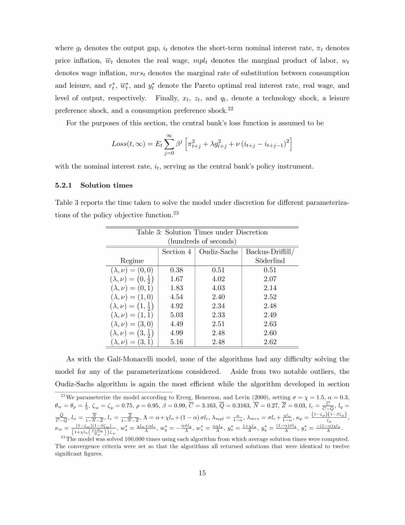
where gt denotes the output gap, it denotes the short-term nominal interest rate, πt denotes

price inflation, wt denotes the real wage, mplt denotes the marginal product of labor, wt

denotes wage inflation, mrst denotes the marginal rate of substitution between consumption

and leisure, and r∗t , w∗t , and y∗t denote the Pareto optimal real interest rate, real wage, and

level of output, respectively. Finally, xt, zt, and qt, denote a technology shock, a leisure

preference shock, and a consumption preference shock.22

For the purposes of this section, the central bank’s loss function is assumed to be

Loss(t,∞) = Et

∞∑

j=0

βj[π2t+j + λg2t+j + ν (it+j − it+j−1)

2]

with the nominal interest rate, it, serving as the central bank’s policy instrument.

5.2.1 Solution times

Table 3 reports the time taken to solve the model under discretion for different parameteriza-

tions of the policy objective function.23

Table 3: Solution Times under Discretion(hundreds of seconds)

Section 4 Oudiz-Sachs Backus-Driffill/Regime Söderlind

(λ, ν) = (0, 0) 0.38 0.51 0.51(λ, ν) =

(0, 12

)1.67 4.02 2.07

(λ, ν) = (0, 1) 1.83 4.03 2.14(λ, ν) = (1, 0) 4.54 2.40 2.52(λ, ν) =

(1, 12

)4.92 2.34 2.48

(λ, ν) = (1, 1) 5.03 2.33 2.49(λ, ν) = (3, 0) 4.49 2.51 2.63(λ, ν) =

(3, 12

)4.99 2.48 2.60

(λ, ν) = (3, 1) 5.16 2.48 2.62

As with the Galí-Monacelli model, none of the algorithms had any difficulty solving the

model for any of the parameterizations considered. Aside from two notable outliers, the

Oudiz-Sachs algorithm is again the most efficient while the algorithm developed in section

22 We parameterize the model according to Erceg, Henerson, and Levin (2000), setting σ = χ = 1.5, α = 0.3,

θw = θp =13, ζw = ζp = 0.75, ρ = 0.95, β = 0.99, C = 3.163, Q = 0.3163, N = 0.27, Z = 0.03, lc =

C

C−Q, lq =

Q

C−Q, ln =

N

1−N−Z, lz =

Z

1−N−Z, Λ = α+χln+(1− α)σlc, λmpl =

α1−α , λmrs = σlc+

χln1−α , κp =

(1−ζp)(1−βζp)ζp

,

κw =(1−ζw)(1−βζw)(1+χln

(1+θwθw

))ζw

, w∗x =χln+αlc

Λ, w∗q = −

ασlq

Λ, w∗z =

αχlzΛ, y∗x =

1+χlnΛ

, y∗q =(1−α)σlq

Λ, y∗z =

−(1−α)χlzΛ

.

23 The model was solved 100,000 times using each algorithm from which average solution times were computed.The convergence criteria were set so that the algorithms all returned solutions that were identical to twelvesignificant figures.

15

4 is typically the slowest, taking on average 1.5 hundreds of a second longer the obtain the

solution. While all of the algorithms are notably slower when solving the EHL model than

when solving the Galí-Monacelli model, the relative inefficiency of the structural form method

is more apparent here because the EHL model contains a larger number of non-predetermined

variables, whose lagged values are all treated as candidate state variables by the algorithm.

Table 4: Solution Times under Commitment(hundreds of seconds)

Section 3 Backus-Driffill Söderlind

Regime Binder-Pesaran Real-QZ Dyn. Prog. Real-QZ

(λ, ν) = (0, 0) 2.81 0.26 — 0.10(λ, ν) =

(0, 12

)0.91 0.32 1.18 0.16

(λ, ν) = (0, 1) 1.07 0.35 1.18 0.15(λ, ν) = (1, 0) 2.06 0.27 — 0.06(λ, ν) =

(1, 12

)1.82 0.29 1.23 0.12

(λ, ν) = (1, 1) 1.77 0.30 2.08 0.13(λ, ν) = (3, 0) 2.93 0.25 — 0.07(λ, ν) =

(3, 12

)3.22 0.30 1.48 0.12

(λ, ν) = (3, 1) 3.26 0.31 1.51 0.12

Table 4 reports computation times for the EHL model when solving for optimal commit-

ment policies; several interesting results emerge. First, the computation time is longer when

a recursive method is used, such as the Backus-Driffill algorithm or Binder and Pesaran’s

RE solution method. Second, optimal commitment policies can generally be obtained more

quickly than optimal discretionary policies, even if a recursive method is used to solve for the

optimal commitment policy. Third, as earlier, the Backus-Driffill algorithm is unable to solve

for the optimal commitment policy when ν = 0, but now none of the other algorithms have

problems.

5.3 A larger model

The final model that we consider is the well-known model developed by Fuhrer and Moore

(1995). The particular specification that we analyze comes from Fuhrer (1997, Table IV).

16

The model equations are given by

yt = 1.45yt−1 − 0.47yt−2 − 0.34ρt−1 + ǫt

ρt =40

41Etρt+1 +

1

41(it −Etπt+1)

pt = 0.42wt + 0.31wt−1 + 0.19wt−2 + 0.08wt−3

πt = 4(pt − pt−1)

vt = 0.42wt + 0.31wt−1 + 0.19wt−2 + 0.08wt−3

wt = 0.42vt + 0.31Etvt+1 + 0.19Etvt+2 + 0.08Etvt+3

+0.002 (0.42yt + 0.31Etyt+1 + 0.19Etyt+2 + 0.08Etyt+3) + εt,

where yt represents the output gap, pt represent the price level, wt represents the nominal

wage, πt represents inflation, wt represents the real wage, ρt represents the real yield on a

ten-year bond, and it, the short-term nominal interest rate, serves as the central bank’s policy

instrument.

Unlike the optimization-based models analyzed above, which each contained only two

endogenous state variables, the Fuhrer-Moore model contains seven endogenous state variables,

and it also contains a relatively large number of non-predetermined variables. Despite its

larger size, the Fuhrer-Moore model can easily be written in second-order structural form and

solved using the algorithms developed in sections 3 and 4. As earlier, the central bank’s loss

function takes the form

Loss(t,∞) = Et

∞∑

j=0

βj[π2t+j + λy2t+j + ν (it+j − it+j−1)

2].

Table 5 reports the time taken (in hundreds of seconds) to solve the Fuhrer-Moore model

using the algorithms presented in section 3 and 4 for different values of λ and ν. The discount

factor, β, is set to 0.99.24

24 The model was solved 10,000 times using each algorithm from which average solution times were computed.

17

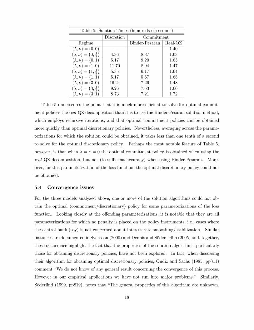
Table 5: Solution Times (hundreds of seconds)

Discretion Commitment

Regime Binder-Pesaran Real-QZ

(λ, ν) = (0, 0) — — 1.40(λ, ν) =

(0, 12

)4.36 8.37 1.63

(λ, ν) = (0, 1) 5.17 9.20 1.63(λ, ν) = (1, 0) 11.70 8.94 1.47(λ, ν) =

(1, 12

)5.35 6.17 1.64

(λ, ν) = (1, 1) 5.17 5.57 1.65(λ, ν) = (3, 0) 16.24 7.26 1.48(λ, ν) =

(3, 12

)9.26 7.53 1.66

(λ, ν) = (3, 1) 8.73 7.21 1.72

Table 5 underscores the point that it is much more efficient to solve for optimal commit-

ment policies the real QZ decomposition than it is to use the Binder-Pesaran solution method,

which employs recursive iterations, and that optimal commitment policies can be obtained

more quickly than optimal discretionary policies. Nevertheless, averaging across the parame-

terizations for which the solution could be obtained, it takes less than one tenth of a second

to solve for the optimal discretionary policy. Perhaps the most notable feature of Table 5,

however, is that when λ = ν = 0 the optimal commitment policy is obtained when using the

real QZ decomposition, but not (to sufficient accuracy) when using Binder-Pesaran. More-

over, for this parameterization of the loss function, the optimal discretionary policy could not

be obtained.

5.4 Convergence issues

For the three models analyzed above, one or more of the solution algorithms could not ob-

tain the optimal (commitment/discretionary) policy for some parameterizations of the loss

function. Looking closely at the offending parameterizations, it is notable that they are all

parameterizations for which no penalty is placed on the policy instruments, i.e., cases where

the central bank (say) is not concerned about interest rate smoothing/stabilization. Similar

instances are documented in Svensson (2000) and Dennis and Söderström (2005) and, together,

these occurrence highlight the fact that the properties of the solution algorithms, particularly

those for obtaining discretionary policies, have not been explored. In fact, when discussing

their algorithm for obtaining optimal discretionary policies, Oudiz and Sachs (1985, pp311)

comment “We do not know of any general result concerning the convergence of this process.

However in our empirical applications we have not run into major problems.” Similarly,

Söderlind (1999, pp819), notes that “The general properties of this algorithm are unknown.

18

Practical experience suggests that it is often harder to find the discretionary equilibrium than

the commitment equilibrium. It is unclear if this is due to the algorithm.”

The approach taken in this paper provides insights as to why, and under what circum-

stances, convergence problems may be encountered when solving for optimal discretionary

policies. For this purpose, the key equations in the algorithm are

P = W+ βF′1QF1 + βH′1PH1 (35)

D = A0 −A2H1 −A4F1 (36)

H1 = D−1(I−A3

(Q+A′3D

−1PD−1A3)−1

A′3D′−1PD−1

)A1 (37)

where (35) and (36) are taken directly from section 4 and (37) is obtained by substituting

(28) into (30). By inspection, difficulties obtaining the optimal discretionary policy can arise

when:

1. The discount factor is close to one and the H1 matrix associated with the optimal

discretionary policy has a spectral radius close to one. In this situation it take a long

time for recursive methods to obtain the fixed point P. If this problem occurs, it may

be useful to solve for P using a non-recursive method, such as the Hessenberg-Schur

algorithm described in Anderson, et al. (1996).

2. The iterations produce a D matrix that is singular. Because A2 and A4 are typically

sparse and A0 has full rank, a singularity in D is unlikely to occur.

3. The iterations produce a(Q+A′3D

−1PD−1A3)

matrix that is singular. This will occur

if both Q and PD−1A3 equal null matrices, i.e. if the loss function does not penalize

movements in the policy instrument(s) and the target variables are contemporaneously

unaffected by movements in the policy instruments. When both PD−1A3 and Q equal

null matrices the optimal discretionary policy is not uniquely determined by setting the

derivative of the loss function with respect to the policy instrument(s) to zero, see (24).

Among these three situations, the first will likely increase the computation time, the second

is very unlikely to occur, and the third accounts for the problems encountered above, in

Svensson (2000), and in Dennis and Söderström (2005), which all involve a loss function that

does not penalize the policy instrument. In fact, the assumption that Q is positive definite

— rather than just positive semi-definite —, which would preclude this problem, is standard

in linear-quadratic control theory (Rustem and Zarrop, 1979; Anderson, et al. 1996, pp175).

19

We did not restrict Q to be positive definite in our analysis because policies where the central

bank (say) does not smooth or stabilize interest rates are of broad interest and can be obtained

for many models.

6 CONCLUSION

This paper has presented new algorithms to solve for optimal commitment rules and optimal

discretionary rules in rational expectation models. These algorithms differ from those devel-

oped by Oudiz and Sachs (1985), Backus and Driffill (1986), and Söderlind (1999) in that they

do not require the optimization constraints to be written in state-space form. This paper has

also extended the class of models that can be analyzed, allowing expectations of future policy

instruments to enter the optimization constraints, which can be useful when solving models

that contain an interest rate term structure, and showed how to derive the Euler equation for

the optimal discretionary policy, which is needed to study targeting rules.

After setting up the optimization problem in section 2, the approaches taken to solve for

optimal commitment policies and optimal discretionary policies were described in sections 3

and 4, respectively. Section 5 took two optimization-based New Keynesian models and used

a range of solution algorithms to solve them for optimal commitment policies and optimal

discretionary policies for a variety of policy objective functions. For these models it was

feasible to analytically derive state-space representations. While the relative advantage of the

solution methods developed in this paper is that they save the user from having to manipulate

a model into state-space form, computational experiments on these small-scale models showed

that the state-space solution methods are generally more efficient, precisely because they

exploit more of the model’s structure. Nevertheless, the methods developed here can be

employed to solve larger models and for small models they are efficient enough to be used in

estimation exercises, which may involve a model being solved many times within a hill-climbing

routine (see Dennis, 2004b, for an application). Section 5 also solved the Fuhrer-Moore model,

a model that can be much more quickly expressed in structural form than in a state-space

form.

The paper has also discussed some of the computational problems that can be encountered

when solving for optimal policies and showed why, in practice, placing a small penalty on

movements in the policy instrument(s), invariably overcomes these problems. These experi-

ments also showed that it is generally more efficient to solve for optimal commitment policies

by solving the underlying rational expectations model using the real QZ-decomposition rather

20

than either the complex QZ-decomposition or the Binder-Pesaran algorithm.

A APPENDIX

A.1 Mathematical preliminary

Assume that 0 < β < 1 and that the spectral radius of the matrix θ is less than one, then

the infinite series S =∞∑j=0

βjθ′jWθj is convergent. Consequently, βθ′Sθ =∞∑j=1

βjθ′jWθj =

S−W, and S can be found as the fixed point of S =W+ βθ′Sθ.

A.2 Establishing Remark 2

Let zt ≡

λtytxt

and K ≡

0 0 0

0 W 0

0 0 Q

. From (27) the recursive equilibrium law of motion

for zt can be expressed as zt =Hzt−1 +Gvt. Given this law of motion, we have

Loss (t,∞) = Et

∞∑

j=0

βjz′

t+jKzt+j

=

z′t

∞∑

j=0

βjH′jKHj

zt +

β

1− β

∞∑

j=0

βjtr(G

′

H′j1KH

j1GΩ

) ,

which using the result regarding convergent infinite series in Appendix A1 can be simplified

to

Loss (t,∞) =

[z′tPzt +

β

1− βtr(G′PGΩ

)],

where P ≡ K+ βH′PH. Finally, again using the law of motion for zt we obtain

Loss (t,∞) =

[z′t−1H

′

PHzt−1 + v′

tG′

PGvt +β

1− βtr(G′PGΩ

)],

as required.

A.3 Establishing Remark 3

From Appendix A2 the loss function under commitment can be written as

Loss (t,∞) =

[z′tPzt +

β

1− βtr(G′PGΩ

)], (A.1)

where P ≡ K+ βH′PH, and the economy’s evolution is given by

zt =Hzt−1 +Gvt. (A.2)

21

From A.2 the unconditional variance-covariance matrix for zt is the fixed point of

Σ =HΣH′ +GΩG′, (A.3)

from which the unconditional variance-covariance matrix for[y′

t x′

t

]′, Φ, can be obtained.

Multiplying A.1 through by (1− β) gives

(1− β)Loss (t,∞) = (1− β) z′tPzt + βtr(G′PGΩ

)

= (1− β) z′tPzt + βtr(PGΩG′

).

Now employing A.3 we have

(1− β)Loss (t,∞) = (1− β) z′tPzt + βtr[P(Σ−HΣH′

)]

= (1− β) z′tPzt + βtr(PΣ

)− βtr

(H′PHΣ

)

= (1− β) z′tPzt + βtr(PΣ

)− tr

[(P− K

)Σ]

= (1− β) z′tPzt − (1− β) tr(PΣ

)+ tr

(KΣ

).

Provided the spectral radius of H is less than one, P will remain bounded even in the

limit as β ↑ 1. Therefore, limβ↑1

Loss (t,∞) = tr(KΣ

). However, defining K ≡

[W 0

0 Q

]so

that K ≡

[0 0

0 K

]only the elements in Σ associated with yt and xt (i.e., Φ) are relevant.

Consequently, we have limβ↑1

Loss (t,∞) = tr (KΦ), as required.

B APPENDIX

B.1 Deriving equation (21)

We show that

Loss (t,∞) = Et

∞∑

j=0

βj(y′t+jWyt+j + x

′t+jQxt+j

)

= y′tPyt + x′tQxt +

β

1− βtr[(F′2QF2 +H

′2PH2

)Ω],

where P ≡ S+ βR =W+ βF′1QF1 + βH′1PH1.

To establish this equality we exploit the properties of convergent geometric series, and the

requirement that, in equilibrium, yt+j =H1yt+j−1+H2vt+j , and xt+j = F1yt+j−1+F2vt+j ,

22

∀ j > 0. First write

Et

∞∑

j=0

βj(y′t+jWyt+j + x

′t+jQxt+j

)= x′tQxt +Et

∞∑

j=0

βj(y′t+jWyt+j

)

+Et

∞∑

j=1

βj(x′t+jQxt+j

). (B.1)

The first term on the RHS of B1 is in the appropriate form. We will treat the second and

third terms on the RHS separately, beginning with the second term. We can write

Et

∞∑

j=0

βj(y′t+jWyt+j

)= y′t

∞∑

j=0

βjH′j1WH

j1

yt

+β∞∑

l=0

∞∑

j=0

β(l+j)tr(H′2H

′l1WHl

1H2Ω).

Assuming that the spectral radius of H1 is less than one, the result in Appendix A1 leads to

Et

∞∑

j=0

βj(y′t+jWyt+j

)= y′tSyt +

β

1− βtr(H′2SH2Ω

), (B.2)

where S ≡W+ βH′1SH1.

Turning to the third term on the RHS of B.1

Et

∞∑

j=1

βj(x′t+jQxt+j

)= βy′t

∞∑

j=0

βjH′j1F

′1QF1H

j1

yt

+β

∞∑

l=0

∞∑

j=0

β(l+j)tr(H′l2F

′1QF1H

l2Ω).

Again, provided the spectral radius of H1 is less than one, the result in Appendix A1 gives

R ≡ F′1QF1 + βH′1RH1. Therefore,

Et

∞∑

j=1

βj(x′t+jQxt+j

)= βy′tRyt +

β

1− βtr(F′2QF2Ω

)+

β2

1− βtr(H′2RH2Ω

). (B.3)

Substituting B.2 and B.3 back into B.1 gives

Loss (t,∞) = y′t (S+ βR)yt + x′tQxt +

β

1− βtr(F′2QF2Ω

)

+β

1− βtr[H′2 (S+ βR)H2Ω

].

Finally, let P ≡ S+ βR =W+ βF′1QF1 + βH′1PH1 giving

Loss (t,∞) = y′tPyt + x′tQxt +

β

1− βtr(F′2QF2Ω

)+

β

1− βtr(H′2PH2Ω

),

23

or

Loss (t,∞) = y′tPyt + x′tQxt +

β

1− βtr[(F′2QF2 +H

′2PH2

)Ω],

as required.

B.2 Establishing Remark 5

Let zt ≡[y′t x′t

]′, then the policy objective function, B.1, can be written as

Loss (t,∞) = Et

∞∑

j=0

βjz′t+jKzt+j, (B.4)

where K ≡

[W 0

0 Q

], and

zt+j =

[H1 0

F1 0

]zt+j−1 +

[H2

F2

]vt+j ≡Hzt+j−1 +Gvt+j , ∀j > 0. (B.5)

Employing B.5 in B.4 gives

Loss (t,∞) = Et

∞∑

j=0

βjz′t+jKzt+j

= z′t

∞∑

j=0

βjH′jKHj

zt +

β

1− β

∞∑

j=0

βjtr(G′H′jKHjGΩ

).

Now, exploiting the properties of convergent geometric series from Appendix A1, we have

Loss (t,∞) = z′tPzt +β

1− βtr(G′PGΩ

),

or

Loss (t,∞) = z′t−1H′

PHzt−1 + v′

tG′

PGvt +β

1− βtr(G′PGΩ

),

where P ≡K+ βH′PH, as necessary.

B.3 Establishing Remark 6

In this appendix we establish that limβ↑1(1− β)Loss (t,∞) = tr (KΦ). Recall that the policy

objective function can be written as

Loss (t,∞) = y′tPyt + x′tQxt +

β

1− βtr[(F′2QF2 +H

′2PH2

)Ω],

24

whereP ≡W+βF′1QF1+βH′1PH1. The components of the unconditional variance-covariance

matrices for yt and xt are given by

Φy = H1ΦyH′1+H2ΩH

′2 (B.6)

Φx = F1ΦyF′1+F2ΩF

′2 (B.7)

Φyx = H1ΦyF′1+H2ΩF

′2

Φxy = F1ΦyH′1+F2ΩH

′2.

Scaling the policy objective function by (1− β) gives

(1− β)Loss (t,∞) = (1− β)(y′tPyt + x

′tQxt

)+ βtr

[(F′2QF2 +H

′2PH2

)Ω].

Exploiting the properties of the trace operator results in

(1− β)Loss (t,∞) = (1− β)(y′tPyt+x

′tQxt

)+ βtr

(QF2ΩF

′2 +PH2ΩH

′2

).

Employing B.6 and B.7 gives

(1− β)Loss (t,∞) = (1− β)(y′tPyt + x

′tQxt

)

+βtr[Q(Φx−F1ΦyF

′1

)+P

(Φy−H1ΦyH

′1

)]

= (1− β)(y′tPyt + x

′tQxt

)

+βtr[QΦx +WΦy − (1− β)

(F′1QF1 +H

′1PH1

)].

Because the spectral radius of H1 is less than one, P remains bounded even as β ↑ 1. Thus,

limβ↑1(1− β) (y′tPyt + x

′tQxt) = 0 and lim

β↑1(1− β) (F′1QF1 +H

′1PH1) = 0, which gives us the

result that limβ↑1(1− β)Loss (t,∞) = tr (QΦx +WΦy) = tr (KΦ), where Φ ≡

[Φy ΦyxΦxy Φx

].

References

[1] Amman, H. and D. Kendrick (1999) Linear quadratic optimization for models with ra-

tional expectations. Macroeconomic Dynamics 3, 534-543.

[2] Anderson, E. Hansen, L. McGrattan, E. and T. Sargent (1996) Mechanics of forming

and estimating dynamic linear economies. in Amman, H. Kendrick, D. and J. Rust (eds)

Handbook of Computational Economics, Volume 1, Chapter 4, North Holland, New York.

[3] Anderson, G. and G. Moore (1985) A linear algebraic procedure for solving linear perfect

foresight models. Economics Letters 17, 247-252.

25

[4] Backus, D. and J. Driffill (1986) The consistency of optimal policy in stochastic rational

expectations models. Centre for Economic Policy Research Discussion Paper #124.

[5] Binder, M. and H. Pesaran (1995) Multivariate rational expectations models and macro-

economic modeling: a review and some new results. in Pesaran, H. and M. Wickens (eds)

Handbook of Applied Econometrics, Blackwell Publishers.

[6] Blake, A. (2004) Open loop time consistency for linear rational expectations models.

Economics Letters 82, 21-27.

[7] Calvo, G. (1983) Staggered prices in a utility-maximizing framework. Journal of Monetary

Economics 12, 383-398.

[8] Chen, B. and P. Zadrozny (2002) An alternative feedback solution for the infinite-horizon,

linear-quadratic, dynamic, Stackelberg game. Journal of Economic Dynamics and Control

26, 1397-1416.

[9] Christiano, L. (2002) Solving dynamic equilibrium models by a method of undetermined

coefficients. Computational Economics 20, 21-55.

[10] Clarida, R. Galí, J. and M. Gertler (1999) The science of monetary policy: a new Key-

nesian perspective. Journal of Economic Literature 37, 1661-1707.

[11] Currie, D. and P. Levine (1985) Macroeconomic policy design in an interdependent world.

in Buiter, W. and R. Marston (eds) International Economic Policy Coordination, Cam-

bridge University Press, Cambridge.

[12] Currie, D. and P. Levine (1993) Rules, Reputation and Macroeconomic Policy Coordina-

tion, Cambridge University Press.

[13] Dennis, R. (2004a) Solving for optimal simple rules in rational expectations models. Jour-

nal of Economic Dynamics and Control 28, 1635-1660.

[14] Dennis, R. (2004b) Inferring policy objectives from economic outcomes. Oxford Bulletin

of Economics and Statistics 66, 735-764.

[15] Dennis, R. and U. Söderström (2005) How important is precommitment for monetary

policy. Journal of Money, Credit, and Banking, forthcoming.

26

[16] Diaz-Gimenez, J. (1999) Linear quadratic approximations: an introduction. in Marimon,

R. and A. Scott (eds) Computational Methods for the Study of Dynamic Economies,

Oxford University press, Oxford, United Kingdom.

[17] Erceg, C. Henderson, D. and A. Levin (2000) Optimal monetary policy with staggered

wage and price contracts. Journal of Monetary Economics 46, 281-313.

[18] Fuhrer, J. (1997) Inflation/output variance trade-offs and optimal monetary policy. Jour-

nal of Money, Credit, and Banking 29, 214-234.

[19] Fuhrer, J. and G. Moore (1995) Inflation persistence. Quarterly Journal of Economics

110, 127-159.

[20] Galí, J. and T. Monacelli (2005) Monetary policy and exchange rate volatility in a small

open economy. Review of Economic Studies, 72, pp707-734.

[21] Giannoni, M. and M. Woodford (2002) Optimal interest-rate rules: I. General Theory.

Princeton University mimeo.

[22] Holly, S. and A. Hughes-Hallett (1989) Optimal Control, Expectations and Uncertainty,

Cambridge University press, Cambridge, United Kingdom.

[23] Jensen, C. and B. McCallum (2002) The non-optimality of proposed monetary policy

rules under timeless perspective commitment. Economics Letters 77, 163-168.

[24] King, R. and M. Watson (2002) System reduction and solution algorithms for singular

linear difference systems under rational expectations. Computational Economics 20, 57-

86.

[25] Klein, P. (2000) Using the generalized Schur form to solve a multivariate linear rational

expectations model. Journal of Economic Dynamics and Control 24, 1405-1423.

[26] Krusell, P. Quadrini, V. and J-V. Rios-Rull (1997) Politico-economic equilibrium and

economic growth. Journal of Economic Dynamics and Control 21, 243-272.

[27] Kydland, F. and E. Prescott (1977) Rules rather than discretion: the inconsistency of

optimal plans. Journal of Political Economy 87, 473-492.

[28] Kydland, F. and E. Prescott (1980) Dynamic optimal taxation, rational expectations and

optimal control. Journal of Economic Dynamics and Control 2, 79-91.

27

[29] McCallum, B. (1999) Solutions to linear rational expectations models: a compact expo-

sition. Economics Letters 61, 143-147.

[30] Orphanides, A. and V. Wieland (1998) Price stability and monetary policy effectiveness

when nominal interest rates are bounded at zero. Board of Governors of the Federal

Reserve, Finance and Economics Discussion Paper#1998-35.

[31] Oudiz, G. and J. Sachs (1985) International policy coordination in dynamic macroeco-

nomic models. in Buiter, W. and R. Marston (eds) International Economic Policy Coor-

dination, Cambridge University Press, Cambridge, 275-319.

[32] Rustem, B. and M. Zarrop (1979) A Newton-type method for the optimization and control

of non-linear econometric models. Journal of Economic Dynamics and Control 1, 283-300.

[33] Sims, C. (2002) Solving linear rational expectations models. Computational Economics

20, 1-20.

[34] Söderlind, P. (1999) Solution and estimation of RE macromodels with optimal policy.

European Economic Review 43, 813-823.

[35] Svensson, L. (2000) Open-economy inflation targeting. Journal of International Eco-

nomics 50, 155-183.

[36] Svensson, L. (2003) What is wrong with Taylor rules? Using judgement in monetary

policy through targeting rules. Journal of Economic Literature June, 426-477.

[37] Taylor, J. (1999) Monetary Policy Rules. University of Chicago Press, Chicago.

[38] Uhlig, H. (1999) A toolkit for analysing nonlinear dynamic stochastic models easily.

in Marimon, R. and A. Scott (eds) Computational Methods for the Study of Dynamic

Economies, Oxford University Press, New York.

[39] Woodford, M. (1999) Commentary: How should monetary policy be conducted in an era

of price stability? Presented at the Symposium on New Challenges for Monetary Policy,

organized by the Federal Reserve Bank of Kansas City at Jackson Hole, Wyoming, August

26-28.

[40] Woodford, M. (2002) Interest & Prices. Princeton University Press, Princeton, New Jer-

sey.

28