OPTIMAL TRANSACTION FILTERS UNDER TRANSITORY TRADING OPPORTUNITIES:

Theory and Empirical Illustration∗

Ronald Balvers and Yangru Wu

September 19, 2008

Forthcoming: Journal of Financial Markets

ABSTRACT If transitory profitable trading opportunities exist, transaction filters mitigate trading costs. We use a dynamic programming framework to design an optimal filter which maximizes after-cost expected returns. The filter size depends crucially on the degree of persistence of trading opportunities, transaction cost, and standard deviation of shocks. For daily dollar-yen exchange trading, the optimal filter can be economically significantly different from a naïve filter equal to the transaction cost. The candidate trading strategies generate positive returns that disappear after transaction costs. However, when the optimal filter is used, returns after costs remain positive and higher than for naïve filters. Keywords: Transaction Costs, Transaction Filters, Trading Strategies, Foreign Exchange JEL Codes: G10, G15, G11

∗ Ronald Balvers: Division of Economics and Finance, College of Business, West Virginia University, Morgantown, WV 26506, and Chinese Academy of Finance and Development, Central University of Finance and Economics, rbalvers@wvu.edu, phone 304-293-7880, fax 304-293-2233; Yangru Wu: Rutgers Business School-Newark & New Brunswick, Rutgers University, Newark, NJ 07102, and Chinese Academy of Finance and Development, Central University of Finance and Economics, yangruwu@andromeda.rutgers.edu, phone 973-353-1146, fax 973-353-1233. We would like to thank Gershon Alperovich, Ake Blomqvist, Ivan Brick, Justin Chan, Sris Chatterjee, N. K. Chidambaran, Chong Tze Chua, Charles Engel, Aditya Goenka, Sam Henkel, Dong Hong, Lixin Huang, Qiang Kang, James Lothian, Paul McNelis, Salih Neftci, Darius Palia, Andrew Rose, Menahem Spiegel, John Wald, Yonggan Zhao, the editor (Bruce Lehmann), the anonymous referee, and seminar participants at the Financial Management Association International, the Pacific Basin Finance, Economics and Accounting Conference, the China International Conference in Finance, Fordham University, Nanyang Technological University, the National University of Singapore, Peking University, Rutgers University, Singapore Management University and the University of Hong Kong for helpful conversations and comments. Yangru Wu would like to thank the Whitcomb Center at the Rutgers Business School and the Office of Research of Singapore Management University for financial support. Part of this work was completed while Yangru Wu visited Singapore Management University and the Central University of Finance and Economics. He would like to thank these institutions for their hospitality. We are solely responsible for any remaining errors.

1

OPTIMAL TRANSACTION FILTERS UNDER TRANSITORY TRADING OPPORTUNITIES:

Theory and Empirical Illustration

September 19, 2008 ABSTRACT If transitory profitable trading opportunities exist, transaction filters mitigate trading costs. We use a dynamic programming framework to design an optimal filter which maximizes after-cost expected returns. The filter size depends crucially on the degree of persistence of trading opportunities, transaction cost, and standard deviation of shocks. For daily dollar-yen exchange trading, the optimal filter can be economically significantly different from a naïve filter equal to the transaction cost. The candidate trading strategies generate positive returns that disappear after transaction costs. However, when the optimal filter is used, returns after costs remain positive and higher than for naïve filters. Keywords: Transaction Costs, Transaction Filters, Trading Strategies, Foreign Exchange JEL Codes: G10, G15, G11

Introduction

It is inarguable that opportunities for above-normal returns are available to market participants at

some level. These opportunities may be exploitable for instance at an intra-daily frequency as a reward for

information acquisition when markets are efficient, or at a lower frequency to market timers when markets

are inefficient. By nature these profit opportunities are predicable but transitory, and transaction costs may

be a major impediment in exploiting them.1 This paper explores the optimal trading strategy when

transitory opportunities exist and transactions are costly.

The model we present is applicable to the arbitrage of microstructure inefficiencies that require

frequent and timely transactions, which may be largely riskless. An example is uncovered interest

speculation in currency markets where a trader takes either one side of the market or the reverse.

Alternatively, a trader arbitrages differences between an asset’s return and that of one of its derivatives:

going long on the arbitrage position or reversing the position and going short, as is the case in covered

interest arbitrage.

1 For instance, Grundy and Martin (2001) express doubt that the anomalous momentum profits survive transaction costs, and Hanna and Ready (2005) find that the momentum profits are substantially reduced when transactions costs are accounted for. Lesmond et al. (2004) conclude more strongly that momentum profits with transactions costs are illusory. Neely and Weller (2003) reach a similar conclusion for trading profits in foreign exchange markets after transaction costs.

2

Alexander (1961) and Fama and Blume (1966) introduced “filter rules” according to which traders

buy (sell) an asset only if its current price exceeds (is below) the previous local minimum (maximum) by

more than X (more than Y) percent, where X and Y are parameters of the rule, commonly set equal and

chosen in the range of 0.5 to 5 percent (see, for instance, Sweeney (1986)). The parameters X (and Y if

different) determine a “band of inactivity” that prompts one to trade once a realization exceeds the local

minimum or is below the local maximum by a certain percentage. A larger band of inactivity (larger X)

filters out more trades, thus reducing transactions costs.2 The general idea of filters, in filter rules as well

as other trading rules, is that if the trade indicator is weak the expected return from the transaction may not

compensate for the transaction cost. Lehmann (1990) provides an interesting alternative filter by varying

portfolio weights according to the strength of the return indicators – in trading smaller quantities of the

assets with the weaker trade indicators, transaction costs are automatically reduced relative to the payoff.

Knez and Ready (1996) and Cooper (1999) explore different filters and find that the after-

transaction-cost returns indeed improve compared to trading strategies with zero filter. The problem with

the filter approach is that there is no way of knowing a priori which filter band is reasonable because the

buy/sell signal and the transaction cost are not in the same units – the filter is the percentage by which the

effective signal exceeds the signal at which a change in position first appears profitable before transaction

costs, but this percentage bears no relation to the percentage return expected. This also implies that there

is no discipline against data mining for researchers: many filters with different bands can be tried to

fabricate positive net strategy returns. While Lehmann’s (1990) approach provides more discipline as it

specifies a unique strategy, the filter it implies is not generally optimal.

The purpose of this paper is to design an optimal filter that a priori maximizes the expected return

net of transaction cost. To accomplish this we employ a “parametric” approach (see for instance Balvers,

Wu, and Gilliland (2000)) that allows the trading signal and the transaction cost to be in the same units. In

2 Note the two usages of the term filter. We distinguish “filter rules” – the specific class of technical trading rules defined above – from a more generic use of the term “filter” – a criterion for selecting a set of trades to exclude. The latter refers typically to a “band of inactivity”. Filter rules use different size filters but filters can be applied to a much broader class of trading rules that are not filter rules. In the following we examine different size filters for ARMA and moving average trading rules, but not for filter rules.

3

effect we convert a filter into returns space and then are able to derive the filter’s optimal band. The

optimal filter depends on the exact balance between maintaining the most profitable transactions and

minimizing the transactions costs.

The optimal filter (band) can be no larger than the transaction cost (plus interest). This is clear

because there is no reason to exclude trades that have an immediate expected return larger than the

transaction cost. In general the optimal filter is significantly smaller than the transaction cost. This occurs

when the expected return is persistent: even if the immediate return from switching is less than the

transaction cost, the persistence of the expected return makes it likely that an additional return is foregone

in future periods by not switching. Roughly, the filter must depend on the transaction cost as well as a

factor related to the probability that a switch occurs. Our model characterizes the determinants of the filter

in general and provides an exact solution for the filter when zero-investment returns have a uniform

distribution.

In exploring the effect of transaction costs when returns are predictable, this paper has the same

objective as Balduzzi and Lynch (1999), Lynch and Balduzzi (2000), and Lynch and Tan (2008).3 The

focus of these authors, however, differs significantly from ours in that they consider the utility effects and

portfolio rebalancing decisions, respectively, in a life cycle portfolio choice framework. They simulate the

welfare cost and portfolio rebalancing decisions given a trader’s constant relative risk aversion utility

function, but they do not provide analytical solutions and it is difficult to use their approach to quantify

the optimal trading strategies for particular applications. Our approach, in contrast, provides specific

theoretical results yielding insights into the factors affecting optimal trading strategies. Moreover our

results can be applied based on observable market characteristics that do not depend on subjective utility

function specifications.

In contrast to Balduzzi and Lynch, Lynch and Balduzzi, and Lynch and Tan, we sidestep the

3 There is a far more extensive literature considering investment choices under transaction costs when returns are not predictable. See Liu and Loewenstein (2002) and Liu (2004) for recent examples. Marquering and Verbeek (2004) assume predictability and adjust for transactions costs. Their approach, however, is a complement to ours in that they integrate risk into the optimal switching choice while accounting for transactions costs after the fact, whereas our approach integrates transactions costs into the optimal switching choice while accounting for risk after the fact.

4

controversial issue of risk in the theory. This simplifies our analysis considerably and is reasonable in a

variety of circumstances. First, we can think of the raw returns as systematic-risk-adjusted returns, with

whichever risk model is considered appropriate. The systematic risk adjustment is sufficient to account for

all risk as long as trading occurs at the margins of an otherwise well-diversified portfolio. Second, in

particular at intra-daily frequencies, traders may create arbitrage positions so that risk is irrelevant. Third,

in many applications risk considerations are perceived as secondary compared to the gains in expected

return; if risk adjustments are relatively small so that the optimal trading rules are approximately correct

then risk corrections can be safely applied to ex post returns.

Our optimal filter will produce higher expected returns than the naïve strategies of either using no

filter or using a transactions-cost-sized filter. We apply the optimal filter to a natural case for our model:

daily foreign exchange trading in the yen/dollar market. As is well-known (see for instance Cornell and

Dietrich (1978), Sweeney (1986), LeBaron (1998), Gencay (1999), and Qi and Wu (2006)), simple

moving-average trading rules improve forecasts of exchange rates and generate positive expected returns

(with or without risk adjustment) in the foreign exchange market. However, for daily trading, returns net

of transaction costs are negative or insignificant if no filter is applied (Neely and Weller (2003)).4

We find that for the optimal filter the net returns are still significantly positive and higher than

those when the filter is set equal to the transaction cost. Further, the optimal filter derived from the theory

given a uniform distribution and two optimal filters derived numerically under normality and

bootstrapping assumptions all generate similar results that are relatively close to the ex post maximizing

filter for actual data. These results are important as they suggest an approach for employing trading

strategies with filters to deal with transactions cost, without inviting data mining. The results also hint that

in some cases the conclusion that abnormal profits disappear after accounting for transaction costs may be

worth revisiting.

The next section develops the theoretical model and provides a general characterization of the

4 Gencay, et al. (2002) show that real time trading models which employ more sophisticated techniques than the simple moving average rules can generate positive cost-adjusted returns with intra-day data.

5

optimal filter for an ARMA(1,1) returns process with general shocks, as well as a specific formula for the

case when the shocks follow the uniform distribution. In section II, we apply the model to uncovered

currency speculation. We show first that the moving-average strategy popular in currency trading can be

related to our ARMA(1,1) specification. We then use the first one-third of our sample to develop estimates

of the returns process which we employ to calculate the optimal filter for an ARMA(1,1), an AR(1), and

two representative MA returns processes. The optimal filter is obtained from the theoretical model for the

uniform distribution but also numerically for the normal distribution and the bootstrapping distribution.

Section III then conducts the out-of-sample test with the final two-thirds of our sample to compare mean

returns from a switching strategy before and after transaction costs. The switching strategies are

conducted under a variety of filters, including the optimal ones, for each of the ARMA(1,1), AR(1), and

MA returns cases. Section IV concludes the paper.

I. The Theoretical Model

A. Autoregressive Conditional Returns and Two Risky Assets

An individual investor maximizes the discounted expected value of an investment over the infinite

horizon. There is a proportional transaction cost and the investor chooses in each period between two

assets that have autocorrelated mean returns. Each period, the investor is assumed to take a zero-cost

investment position: a notional $1 long position in one asset and a notional $1 short position in the other

asset. This implies that any profits or losses do not affect future investment positions. The return on the

zero-cost investment position xt (a $1 long position in asset 1 and a $1 short position in asset 2) is

assumed to follow an ARMA(1,1) process as a parsimonious parameterization of mild return

predictability. Given that either the return on the investment position has no systematic risk or the investor

is risk neutral, the decision problem is

⎥⎦

⎤⎢⎣

⎡⎟⎟⎠

⎞⎜⎜⎝

⎛−

+++−−− c

rxV

rxV

MaxxE=xV tttttttt 2

1),(

,1

),(),( 21

111 1

εεε , (1)

subject to: εεδρ tttt +x = x 11 −− − , ),0(1 δρε Max ,0 = E tt >− (2)

6

Each period, the investor chooses whether to hold a zero-investment position long in asset 1 and short in

asset 2, or the reverse. A proportional transaction cost c is incurred whenever a position is closed out,

implying a cost of 2c when a position is reversed.5 In equation (1), the expected net present value of the

investment strategy denoted by the value function )(⋅iV at time t-1 depends on the state as given by the

existing long position in asset i and short position in the other asset, and the variables describing the

distribution of xt , namely xt 1− and 1−tε . This value equals the current expected return, given the existing

asset position (which we call 1 without loss of generality), plus the expected value in the next period

discounted once at rate r, which depends on the updated return state variables xt and tε as well as the

new zero-investment asset position (i = 1 or 2, whichever maximizes the expected net present value), and

minus the up-front adjustment cost incurred if the zero-investment position is switched from long in asset

1 to long in asset 2. Wealth is not a state variable, because of risk neutrality and the assumption that the

long position in each period is always $1. Assuming that the scale of investment is low enough that

wealth/margin does not become an issue preserves the relative simplicity of the decision problem.

Equation (2) describes the return process xt for the zero-investment position long in asset 1 and

short in asset 2. The ARMA(1,1) process for xt is assumed to be persistent in the sense that xt 1−

positively affects xt ( 0>ρ ) and that 1−tε positively affects xt ( δρ > ). The unconditional mean of xt is

zero and reversing the zero-cost position necessarily generates a return of xt− . Define ttt x E 1−≡µ , and

let it represent, without loss of generality, the conditional expected return of the current zero-investment

position. The disturbance term ε t is symmetric and unimodal, with unbounded support, density )(ε tf ,

and cumulative density )(ε tF . )(⋅V denotes the maximum expected net present value of the strategy

given the existing zero-investment position. Then:

5 Given the assumed risk neutrality, symmetry, and proportional transaction costs, intermediate positions, with investment in both assets or in neither asset, are never optimal.

7

Proposition 1. For the decision problem in equations (1 )and (2) a unique 0*<µ exists

such that the investor maintains the current zero-investment position whenever

*1 µµ >+ t and reverses the position whenever *

1 µµ ≤+ t . The resulting expected net

present value is:

)(21

)()(

1)(

)( 1

*

1

*t

tt

ttt dFc

rV

+ dF r

V + = V

t

t

εµ

εµ

µµδρρµµ

δρρµµ

⎟⎠

⎞⎜⎝

⎛ −+−

⎟⎠

⎞⎜⎝

⎛+

+−−

∞−

+∞

−−

∫∫ , (3)

subject to: = ttt εδρµρµ )(1 −++ , with ),0(1 δρε Max ,0 = E tt >− . (4)

Proof. See Appendix. 　

Equation (3) states that the maximum expected discounted investment return is equal to the

expected return for the current position tµ plus, either the once-discounted maximum expected net

present value of the strategy when the current investment position is maintained, or the once-discounted

maximum expected net present value of the strategy, net of adjustment costs incurred when the current

investment position is reversed. The integral bounds indicate the critical (cutoff) value for the current

disturbance term ε t according to which the investment position is maintained or reversed (higherε t

implies higher future expected return for the existing zero-investment position, so less incentive to

switch). tµ is a sufficient state variable for the individual investor maximizing the expected net present

value from the zero-cost investment positions because equation (2) for the realized zero-investment return

implies equation (4) for the conditional expected zero-investment return, and the latter is the pertinent

variable for the risk-neutral expected value maximizer.

Given that the benefit of switching, the difference between )( µ−V and )(µV , is monotonically

decreasing in µ there is exactly one critical value *µ below which switching is optimal. Intuitively *µ

must be negative because it makes no sense to switch when 1+tµ is zero or positive. Our purpose is to

provide in the following a specific characterization of *µ for empirical purposes.

8

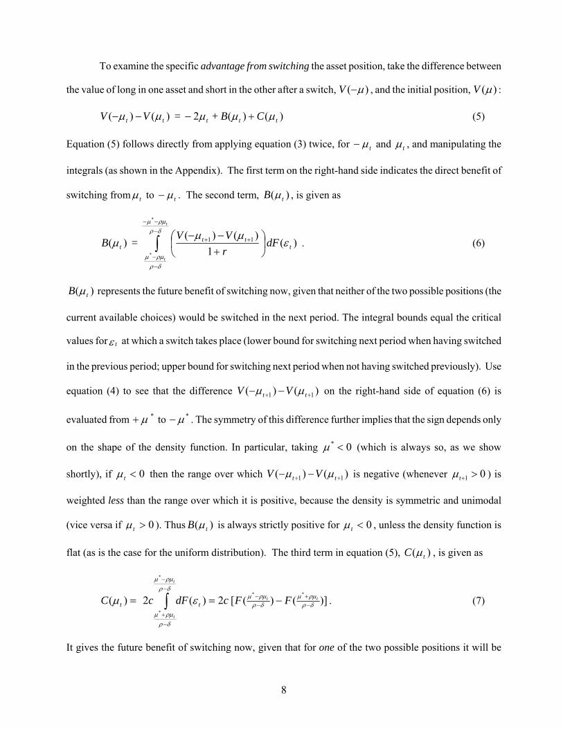
To examine the specific advantage from switching the asset position, take the difference between

the value of long in one asset and short in the other after a switch, )( µ−V , and the initial position, )(µV :

)()(2)()( ttttt CB+ = VV µµµµµ +−−− (5)

Equation (5) follows directly from applying equation (3) twice, for tµ− and tµ , and manipulating the

integrals (as shown in the Appendix). The first term on the right-hand side indicates the direct benefit of

switching from tµ to tµ− . The second term, )( tB µ , is given as

dF rVV

= B ttt

t

t

t

)(1

)()()( 11

*

*

εµµ

µδρρµµ

δρρµµ

⎟⎠

⎞⎜⎝

⎛+−− ++

−−−

−−∫ . (6)

)( tB µ represents the future benefit of switching now, given that neither of the two possible positions (the

current available choices) would be switched in the next period. The integral bounds equal the critical

values forε t at which a switch takes place (lower bound for switching next period when having switched

in the previous period; upper bound for switching next period when not having switched previously). Use

equation (4) to see that the difference )()( 11 ++ −− tt VV µµ on the right-hand side of equation (6) is

evaluated from *µ+ to *µ− . The symmetry of this difference further implies that the sign depends only

on the shape of the density function. In particular, taking 0* <µ (which is always so, as we show

shortly), if 0<tµ then the range over which )()( 11 ++ −− tt VV µµ is negative (whenever 01 >+tµ ) is

weighted less than the range over which it is positive, because the density is symmetric and unimodal

(vice versa if 0>tµ ). Thus )( tB µ is always strictly positive for 0<tµ , unless the density function is

flat (as is the case for the uniform distribution). The third term in equation (5), )( tC µ , is given as

)]()([2)(2)(**

*

*δρρµµ

δρρµµ

δρρµµ

δρρµµ

εµ −+

−−

−−

−+

−== ∫ tt

t

t

FFcdFcC tt . (7)

It gives the future benefit of switching now, given that for one of the two possible positions it will be

9

optimal to switch in the next period (note that it is never optimal for both positions to switch). In that

case, both possible positions end up becoming identical one period later and the only difference is the

transaction cost. )( tC µ represents the expected difference in transaction cost expenditure for the two

positions: the cost times the probability of not switching initially but switching anyway next period minus

the probability of switching initially and then switching back in the next period. Note that, from

inspection of equation (7), )( tC µ must be positive for 0<tµ (and negative for 0>tµ ).

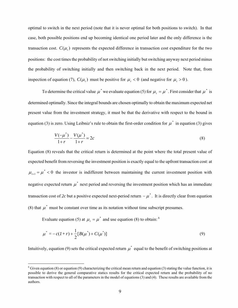
To determine the critical value *µ we evaluate equation (5) for *µµ =t . First consider that *µ is

determined optimally. Since the integral bounds are chosen optimally to obtain the maximum expected net

present value from the investment strategy, it must be that the derivative with respect to the bound in

equation (3) is zero. Using Leibniz’s rule to obtain the first-order condition for *µ in equation (3) gives

* *( ) ( ) 2

1 1V V c

r rµ µ−

− =+ +

(8)

Equation (8) reveals that the critical return is determined at the point where the total present value of

expected benefit from reversing the investment position is exactly equal to the upfront transaction cost: at

0*1 <=+ µµ t the investor is indifferent between maintaining the current investment position with

negative expected return *µ next period and reversing the investment position which has an immediate

transaction cost of 2c but a positive expected next-period return *µ− . It is directly clear from equation

(8) that *µ must be constant over time as its notation without time subscript presumes.

Evaluate equation (5) at *µµ =t and use equation (8) to obtain: 6

1( ) [ ( ) ( )]2

* * * = c 1+ r B Cµ µ µ− + + (9)

Intuitively, equation (9) sets the critical expected return µ* equal to the benefit of switching positions at

6 Given equation (8) or equation (9) characterizing the critical mean return and equation (3) stating the value function, it is possible to derive the general comparative statics results for the critical expected return and the probability of no transaction with respect to all of the parameters in the model of equations (3) and (4). These results are available from the authors.

10

µ* minus the up-front transaction cost (including interest) from switching. The benefit of switching at the

expected returnµ* includes the cost saving of a reduction in the probability of switching next period,

( )*C µ , as well as the expected immediate revenue from the improved asset position, )(µ*B . As

( ) ( ) 0* *B Cµ µ+ > from equations (6) and (7), given that * 0µ < , it follows that * (1 )c rµ− < + . This is

intuitive because, if the current expected return is greater than or equal to the transaction cost, a switch is

clearly beneficial because the end-of-period gain in expected return *2µ− immediately pays for the

transaction cost )1(2 rc + and the switch also improves the potential for future profits.

B. Closed Form Solution for Uniform Innovations

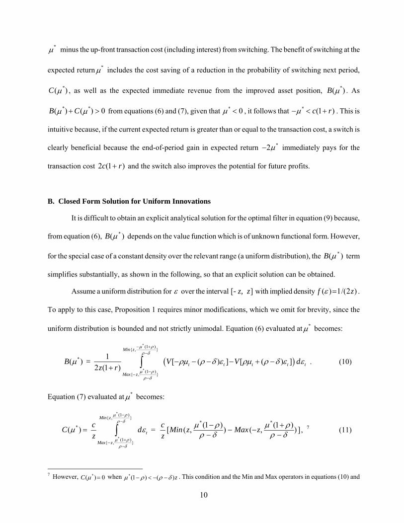
It is difficult to obtain an explicit analytical solution for the optimal filter in equation (9) because,

from equation (6), )( *µB depends on the value function which is of unknown functional form. However,

for the special case of a constant density over the relevant range (a uniform distribution), the )( *µB term

simplifies substantially, as shown in the following, so that an explicit solution can be obtained.

Assume a uniform distribution for ε over the interval ][ z z, - with implied density )2/(1)( zf =ε .

To apply to this case, Proposition 1 requires minor modifications, which we omit for brevity, since the

uniform distribution is bounded and not strictly unimodal. Equation (6) evaluated at *µ becomes:

( )

*

*

(1 ){ , }

*

(1 ){ , }

1( ) [ ( ) ] [ ( ) ]2 (1 )

Min z

t t t t t

Max z

B = V V d z r

µ ρρ δ

µ ρρ δ

µ ρµ ρ δ ε ρµ ρ δ ε ε

− +−

−−

−

− − − − + −+ ∫ . (10)

Equation (7) evaluated at *µ becomes:

*

*

(1 ){ , }

*

(1 ){ , }

( )Min z

t

Max z

cC dz

µ ρρ δ

µ ρρ δ

µ ε

−−

+−

−

= ∫ = ]))1(,())1(,([**

δρρµ

δρρµ

−+−−

−− zMaxzMin

zc

, 7 (11)

7 However, *( ) 0C µ = when z)()1(* δρρµ −−<− . This condition and the Min and Max operators in equations (10) and

11

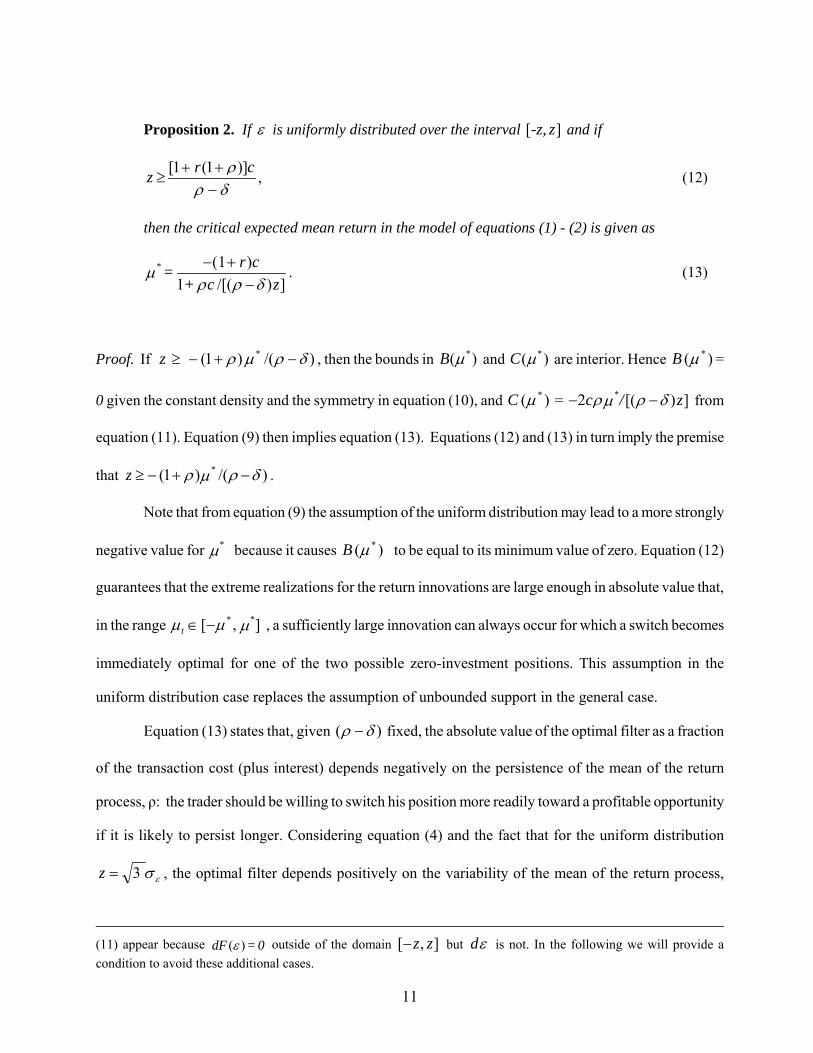
Proposition 2. If ε is uniformly distributed over the interval [ ]-z, z and if

[1 (1 )]r cz ρρ δ

+ +≥

−, (12)

then the critical expected mean return in the model of equations (1) - (2) is given as

(1 )1 /[( ) ]

* r c = + c z

µρ ρ δ− +

−. (13)

Proof. If )/()1( * δρµρ −+−≥z , then the bounds in *( )B µ and *( )C µ are interior. Hence )( *µB =

0 given the constant density and the symmetry in equation (10), and )( *µC = 2 [( ) ]*c / zρ ρ δµ− − from

equation (11). Equation (9) then implies equation (13). Equations (12) and (13) in turn imply the premise

that (1 ) /( )*z ρ ρ δµ≥ − + − . 　

Note that from equation (9) the assumption of the uniform distribution may lead to a more strongly

negative value for *µ because it causes )( *µB to be equal to its minimum value of zero. Equation (12)

guarantees that the extreme realizations for the return innovations are large enough in absolute value that,

in the range *t ],[ * µµµ −∈ , a sufficiently large innovation can always occur for which a switch becomes

immediately optimal for one of the two possible zero-investment positions. This assumption in the

uniform distribution case replaces the assumption of unbounded support in the general case.

Equation (13) states that, given )( δρ − fixed, the absolute value of the optimal filter as a fraction

of the transaction cost (plus interest) depends negatively on the persistence of the mean of the return

process, ρ: the trader should be willing to switch his position more readily toward a profitable opportunity

if it is likely to persist longer. Considering equation (4) and the fact that for the uniform distribution

εσ3=z , the optimal filter depends positively on the variability of the mean of the return process,

(11) appear because 0 = dF )(ε outside of the domain [ , ]z z− but dε is not. In the following we will provide a condition to avoid these additional cases.

12

z)( δρ − , scaled by the transactions cost, c: if the mean is highly variable compared to the transaction

cost, then a trader should require a higher immediate expected return before switching since there is a

higher chance that he may want to switch back soon.

It is instructive to evaluate a few special cases in equation (13). First, if we have a pure MA(1)

process, 0=ρ , then the optimal filter becomes the naïve filter (plus interest), * (1 )c rµ = − + . The reason

is that there is no persistence in the profit opportunities because the current conditional expected return

does not depend on past conditional expected returns. Second, if we have a pure AR(1) process, 0=δ ,

then the optimal filter becomes )]/(1/[)1(* zcrc ++−=µ , which is closer to zero than in the MA(1)

case, implying that a switch occurs more readily (because the conditional expected return is persistent).

Interestingly the filter in the AR(1) case does not depend on ρ . The explanation is that, as ρ increases,

two offsetting effects occur: due to the tρµ term in equation (4) the expected return becomes more

persistent, making the critical expected return less negative, but due to the tρε term in equation (4) the

expected return also changes more rapidly, making the critical expected return more negative.

II. Empirical Illustration for Foreign Exchange Trading: Optimal Filter Calculation

The model developed in the preceding section can be interpreted in three different ways. First, if

we ignore the underlying tx process in equation (2), the tµ in equation (4) may be interpreted as an

excess return that is fully known at time t. Thus, we are dealing with a case of pure arbitrage where the

trader optimizes the after-transaction-cost return )( tV µ . Second, we may think of tµ as the risk-adjusted

expected return, the “alpha”, so that )( tV µ represents the expected net present value adjusted for

systematic risk. Similarly, tµ could represent a particular expected utility level, which would also account

for risk. Third, we can interpret tµ as an expected return in a case where risk is relatively small or non-

systematic. In this case, an appropriate risk correction can simply be applied to the ex post returns. A

minor drawback is that the optimal filter has to be applied with unadjusted returns, but this is not a major

13

issue if the risk adjustment is small and would anyway bias results away from finding positive trading

returns.8

Empirically, it is difficult to find accurate data to examine the first interpretation, while the second

interpretation requires employing a particular risk model. Accordingly, we adopt the third interpretation

of the theory in considering uncovered interest speculation in the dollar-yen spot foreign exchange market.

A. A Parametric Moving Average Trading Strategy

As discussed extensively in the literature, see for instance Cornell and Dietrich (1978), Frankel

and Froot (1990), LeBaron (1998, 1999), Lee and Mathur (1996), Levich and Thomas (1993), Qi and Wu

(2006), Sweeney (1986), and others, profitable trading strategies in foreign exchange markets traditionally

have employed moving-average (MA) technical trading rules.9 MA trading rules of size N work as

follows: calculate the moving average using N lags of the exchange rate. Buy the currency if the current

exchange rate exceeds this average; short-sell the currency if the current exchange rate falls short of this

average.

Defining ts as the log of the current-period spot exchange rate level (dollar price per yen) and

ts∆ as the percentage appreciation of the yen, the implicit exchange rate forecasting model behind the

MA trading rule is

11

1 ]/)[( +=

−+ +⎟⎠

⎞⎜⎝

⎛−=∆ ∑ t

N

iittt Nsss ελ , 0,01 >=+ λε ttE . (14)

For any positive λ, equation (14) implies a positive expected exchange rate appreciation if the log of the

current exchange rate exceeds the N-period MA. Empirically, we find λ to be positive in all our

specifications. Hence, the decision rule based on equation (14) to buy (short) the currency if the expected

8 Neely (2003) finds that optimizing rules based on an ex ante risk criterion provide substantially different results compared to results adjusted for risk ex post. He notes, however, that the ex ante risk adjustment implies higher (adjusted) returns from technical trading. 9 The source of the excess returns from MA strategies in foreign exchange markets may be due to central bank intervention designed to smooth exchange rate fluctuations. See for instance Sweeney (2000) and Taylor (1982). However, recent results by Neely and Weller (2001) and Neely (2002) argue against this perspective.

14

appreciation is positive (negative) leads to a trading strategy equivalent to the MA trading strategy for any

positive value of λ.10 In what follows, our strategy is to transform equation (14) to infer empirically a

value for λ which, in addition to implying identical switch points as the MA rule, also provides a

quantitative estimate of the expected gain from switching that may be compared directly to the

transactions cost.

The true distribution of the exchange rate can be very complex and the simple MA process in

equation (14) can only be an approximation of the true exchange rate process. We are motivated to use

the MA rule because it is the most popular rule studied by researchers and used by practitioners. It is

important to emphasize here that the primary purpose of this paper is not per se to search for the best

exchange rate forecasting model to generate trading profitability, or to explain the potential profitability

from certain trading strategies. But rather, the key point we want to make is that, given a data-generating

process which exhibits some return predictability, an optimal transaction filter can be designed to

maximize the after-cost expected profitability of a particular trading strategy. The optimal filter size is

conditioned on a specific exchange rate forecasting model and can be easily and unambiguously computed

using prior data. It is shown empirically below that the optimal filter can be significantly smaller than the

naïve filter equal to the transaction cost. The optimal filter will in general outperform the naïve filters

regardless of the specific return-generating process assumed.

Equation (14) can straightforwardly be rewritten as an autoregressive process in the percentage

change in the exchange rate, with the coefficients in the autoregression given by the Bartlett weights:

11

01 +

−

=−+ +⎟⎠⎞

⎜⎝⎛∑ ∆

−=∆ t

N

iitt s

NiNs ελ , (15)

Typical studies on technical analysis of foreign exchange do not utilize information on interest

rates in computing the moving averages and do not estimate a parametric model for forecasting. To be

10 Given equation (14) there is a clear link between the popular MA filters with a band and our filter. An exchange rate such that the moving average exchange rate is exceeded by x percent induces a switch. In our case, for a naïve filter equal to c, for instance, we need 2x cλ > to induce a switch. So, for the numbers we find in our empirical section for the MA(21) process, our naïve filter corresponds to 2 /x c λ= = 0.1/0.025 = 4, a 4 percent band for the ad hoc MA filter.

15

fully consistent with our theory, we want to treat the excess return as the variable to be forecasted in the

forecasting equation. To do so, we add the interest rate differential to the percentage change in exchange

rate, so that Equation (15) becomes:

11

01 +

−

=−+ +⎟⎠⎞

⎜⎝⎛∑

−= t

N

iitt x

NiNx ελ , (16)

where USt

JPttt rrsx 11 −− −+∆≡ , JP

tr is the daily Japanese interest rate, and UStr is the daily U.S. interest rate.

In other words, tx denotes the excess return from buying the Japanese yen and shorting the U.S. dollar

(or the deviation from uncovered interest parity).11

In the presence of transaction costs, the MA rule needs to be supplemented with a filter that

indicates by how far the current spot rate must exceed (or fall short of) the MA in order to motivate a

trade. The advantage of equation (16) is that it is parametric and, given an estimate for λ, can provide a

quantitative measure of the filter based on comparing expected return to the transaction cost.

To obtain analytically the optimal filter for the MA criterion in the context of the model it is

necessary that equation (16) be translated to ARMA(1,1) format, for which the model provides the optimal

filter (which is in closed form expression if the tε are uniformly distributed). LeBaron (1992), Taylor

(1992), and others have shown that an ARMA(1,1) well replicates moving average trading rule results.

The theoretical restriction on the ARMA(1,1) process in equation (2) that ),0( δρ Max> is satisfied for all

our empirical specifications. Inverting the ARMA(1,1) process yields an alternative autoregression:

10

( ) it t i i

ix xρ δ δ ε

∞

+ − +=

= − +∑ (17)

Comparing equations (16) and (17) it follows that equation (17) is a good approximation for equation (16)

if we set ρ δ λ− = and if the NiN /)( − terms are close to iδ for all i. Taking a natural log

approximation, and choosing δ to match the Bartlett weights:

)(ln]/)ln[(/ δiNiNNi =−≈− ⇒ )/1exp( N−=δ . (18)

11 Deviations from uncovered interest parity and their persistence are documented in previous research. See, for example, Canova (1991), Engel (1996), and Mark and Wu (1998).

16

Thus, for a given N, we run regression (16) to obtain an estimate of λ . Then from )/1exp( N−=δ and

δλρ += , we can uniquely identify a δ and ρ that provide a good ARMA(1,1) proxy for an MA-based

process with a relatively large N. In turn, the ARMA parameters allow us to calculate analytically the

critical expected return *µ governing the transaction choice.

B. Preliminary Dollar-Yen Process Estimates

Our data on the Japanese yen – U.S. dollar spot exchange rate cover the period from August 31,

1978 to May 3, 2003 with 6195 daily observations. Daily exchange rate data for the Japanese yen are

downloaded from the Federal Reserve’s webpage. For interest rates we obtain the Financial Times’ Euro-

currency interest rates from Datastream International. The first 1/3 of the sample (2065 observations) is

used for model estimation. Out-of-sample forecasting starts on November 28, 1986 until the end of the

sample (4130 observations). We estimate the exchange rate dynamics in four ways: 1. an ARMA(1,1)

process (equation 2); 2. an AR(1) process (δ in equation 2 is set equal to zero); 3. a process consistent

with an MA rule of 21 lags (21 trading days in a month), as is commonly considered with daily data

(equation (16)); and 4. a process consistent with an MA rule of size 126 (half a year), around the size

often used by traders, although results appear to depend little on the size of the MA process chosen

(LeBaron (1998, 1999)). We choose these four models as our empirical illustration for the following

reasons. Model 1, the ARMA(1,1), is the exact model assumed in our theoretical derivation, while Model

2, the AR(1) model, is a more parsimonious specification that is an interesting special case. Models 3 and

4 are commonly employed by academia and practitioners.

Columns (1)-(5) of Table I show the results of the in-sample model estimation using the first 1/3

of our sample for each way of capturing the exchange rate dynamics. For the ARMA(1,1) process we find

ρ = 0.918 and δ = 0.880 with a standard error of εσ = 0.00658; for the AR(1) process we find low

persistence with ρ = 0.0548 and a standard error of εσ = 0.00659. Thus, both processes provide similar

17

accuracy although the parameters differ substantially.12 While the data cannot tell us clearly whether the

AR(1) or the ARMA(1,1) process is better at describing the exchange rate dynamics, we will see that the

implications for optimal trading are substantially different.13 14 For the representative moving average rule

with 21 lags we find for the slope in equation (16) that λ = 0.0257 and εσ = 0.00656. Since we have N

=21 we obtain from equation (18) that ρ = 0.979 and δ = 0.954, which is not statistically distinguishable

from the direct estimates from the ARMA(1,1) model. The MA(126) process yieldsλ = 0.00818 and εσ =

0.00635, implying by approximation that ρ = 0.999 and δ = 0.992.

We assume one round trip transaction cost of 2c = 0.001 (10 basis points) per switch throughout.15

Sweeney (1986) finds a transaction cost of 12.5 basis points for major foreign exchange markets, but more

recent work by Bessembinder (1994), Melvin and Tan (1996), and Cheung and Wong (2000) finds bid-ask

spreads for major exchange rates between 5 and 9 basis points. To account for transaction costs in addition

to those imbedded in the bid-ask spread, related to broker fees and commissions and the lending-

borrowing interest differential, we use 10 basis points as a realistic number for the dollar-yen market. The

daily U.S. interest rate is on average over the first 1/3 of the sample equal to 0.000439 percent. This

average rate is used as a proxy for the discount rate r in computing the optimal filter in equation (13).

12 Previous more elaborate research on this issue by LeBaron (1992) and Taylor (1992) on the other hand finds that , while the ARMA(1,1) formulation does well, the AR(1) case is much poorer in replicating the key features of exchange rate series. 13 Balvers and Mitchell (1997) raise a similar issue in the context of optimal portfolio choice under return predictability. 14 Charles Engel pointed out to us the apparent puzzle that the ARMA(1,1) model 11 880.0918.0 −− −=− tttt xx εε implies a

substantially different optimal filter from our AR(1) model, ttt xx ε+= −1055.0 . This is surprising, given that the AR(1) model can be rewritten as an ARMA(2,1) model 121 863.0047.0918.0 −−− −=+− ttttt xxx εε , which is very similar to the ARMA(1,1) model. The AR(1) and ARMA(1,1) models are similar in that they unconditionally describe the data with roughly the same degree of precision as indicated by εσ in our Table I. The reason they imply quite different filters is because the optimal filter depends on the persistence of the conditional expected return. Equation (4) says that the conditional expected return is an AR(1) process, which becomes εµεµµ 1111 038.0918.0)880.0918.0(918.0 −−−− +=−+= ttttt for our empirical ARMA(1,1) model, while our empirical AR(1) model (or the equivalent ARMA(2,1)) implies εµµ 11 055.0055.0 −− += ttt . We can see that the conditional expected return from the ARMA(1,1) model is much more persistent than that from the AR(1) model. Therefore, we apply a smaller filter for the ARMA(1,1) model since even a small positive expected one-period return is enough to make up for the transaction cost because the new position is likely to remain optimal for a number of future periods. 15 Note that c in the model represents the cost of closing out a zero-investment position. For most assets this requires both a sale and a purchase implying a round trip transaction cost. However, in the case of foreign exchange we directly purchase one currency with the other, implying only a one-way transaction cost. Reversing the position requires double that transaction cost 2c which is one round trip.

18

The true distribution of the exchange rate can be quite complex, and we do not know a priori

which distributional assumption is the best approximation. Therefore we choose to estimate the optimal

filter *µ using three methods. First, under the assumption that the error term tε is uniformly distributed

the optimal filter, denoted *Uµ , can be analytically calculated using equation (13). Second, tε is assumed

to follow a normal distribution. In this case, the result in equation (13) no longer holds, and we estimate

the optimal filter, denoted *Nµ , through Monte-Carlo simulation. Last, we do not make an assumption

about the distribution of tε and estimate the optimal filter, denoted *Bµ , by bootstrapping the model

residuals tε̂ with replacement.

C. The Optimal Filter Implied by the Theory under the Uniform Distribution

Under the assumption of a uniform distribution, we can obtain z from the relation εσ3=z . All

the information now is there to allow us to calculate the optimal filter from equation (13) for the dollar-

yen exchange rate. Column (6) of Table I provides the results. For the AR(1) case we find that the ratio of

the critical return to the transaction cost is * /U cµ− = 0.92.16 Hence, in this case the optimal filter is not

very different from a naïve filter that equals the transaction cost c. The main reason is that, from equation

(4), the persistence in the mean return is small at ρ = 0.0548 so that, no matter what the current holdings

are, there is not much difference in future probabilities of trading.

For the 1-month MA process, the parameters backed out from the MA(21) model yield * /U cµ− =

0.23. Note that inequality (12) is violated, as is necessary here when * /U cµ− < 0.50, implying that the

analytical value obtained from equation (13) is no longer accurate and must be viewed as a good

approximation; hence it is more precise to state that * /U cµ− ≈ 0.23. Intuitively, the slow adjustment in the

conditional mean for these parameter values implies that, in some cases, even the most extreme realization

16 This ratio is the immediate gain of switching to *µ− from *µ (the gain of *2µ− ) divided by the transaction cost 2c.

19

of the exchange rate innovation would not be sufficient to induce switching. Hence, one would be certain

of avoiding transaction costs for at least one period (and likely more) by buying/keeping the exchange

with the positive expected return. This explains the low value of the critical expected return relative to the

transaction cost.

The 6-month MA process, MA(126) yields the smallest filter, * /U cµ− = 0.083. One reason is the

high persistence of expected return (the implied persistence parameter ρ = 0.999). Another is the fact that

by nature the long MA process is very smooth so changes in the mean occur very slowly so that the

number of transactions is small, even when there is no filter. This is a possible reason for the popularity of

this particular trading rule with practitioners.

For our main specification, the ARMA(1,1) case with ρ = 0.918 and δ = 0.880, we find that the

optimal filter is * /U cµ− = 0.32. The reason that this number is so much lower than under the AR(1) case

is clear from equation (4). The persistence is not only high now with ρ = 0.918 but it is also high relative

to the innovation in the conditional mean, given by ( ) ερ δ σ− = εσ038.0 . Hence, it is highly likely that

the exchange position (dollar or yen) with the currently positive expected return is going to be unchanged

in the nearby future.

D. The Optimal Filter Obtained Numerically

As a check on the dependence of the results on the uniform distribution, we also find the optimal

filter numerically using a Monte Carlo approach, assuming normality, and a bootstrapping approach.

For each Monte-Carlo trial, we simulate expected returns tµ using equation (16) with parameters

estimated from the first 1/3 of the sample. We then choose the filter *Nµ which maximizes the after-cost

average excess return. This process is replicated 500 times. Column (7) of Table I reports the median

value of the optimal filter to transaction cost ratio, * /N cµ− , over the 500 Monte-Carlo trials. For each

model, the ratio * /N cµ− is quite close to the optimal ratio implied under the uniform distribution * /U cµ− ,

20

with the difference between them never exceeding 5 percent of the transaction cost.

The actual distribution of tε may be neither uniform nor normal. In this case, we re-sample with

replacement the fitted residuals tε̂ of equation (16) and use model parameters to generate expected return

observations tµ . Similar to the Monte-Carlo experiment, for each bootstrapping trial, the optimal filter is

chosen to be the one which maximizes the after-cost average excess return. Column (8) of Table I reports

the median estimate of the optimal filter to cost ratio * /B cµ− over 500 bootstrapping replications.

Encouragingly, the optimal filters, for the theoretical uniform distribution case and the numerical normal

and bootstrapping cases, are quite similar for each of the returns processes. Thus, the optimal filter value

is robust to distributional assumptions.

Applying the optimal filters to the data in trading on deviations from uncovered interest parity, we

expect straightforwardly that the optimal filters will outperform naïve filters. In particular, we expect that

the optimal filter does better than the naïve “0” filter that is used implicitly when transaction costs are

ignored for trading decisions (but not for calculating returns), because it saves on transaction costs; and

does better than the naïve “c” filter that is employed when trading costs are considered myopically,

because it does not filter out as many profitable transactions.

E. The Filter Obtained Empirically

An alternative, non-theoretical, procedure would establish potential trading strategy profits after

transaction costs based on a prior data sample and for a grid of ratios of the (negative of the) critical

expected return to the transaction cost. We then smooth the graph of the after-transaction-cost trading

strategy profits over the grid and choose the ratio, * /E cµ− , that maximizes the ex post smoothed profits

for the prior sample and apply this filter to out of sample data. This empirical procedure uses the in-

sample part of the data more intensively, not just to estimate the time-series parameters but also the

empirically optimal filter. However, the chosen filter depends on the smoothing procedure, and the

intensive use of the in-sample data may hurt if that sample is not representative enough of the full data.

21

As before, we use the first 1/3rd of the sample as the prior sample. We use the first ½ of the prior

sample to obtain the initial model estimates and then roll forward to the end of the prior sample,

calculating the after-cost profits for a grid of values of / cµ− over the feasible range [0, 1.2] in

increments of 0.02. The profit function is then smoothed using a 5th order moving average (the average of

2 leads, the current value, and 2 lags) filter and we pick the value of / cµ− maximizing the smoothed

profits as the filter * /E cµ− , to be applied out of sample.

The filters * /E cµ− obtained in this way are shown in figures 1-4 (we do not report the

accompanying results in Table II to save space).17 These filters are relatively close to the theoretical

filters for the ARMA(1,1) case and the two MA cases, and generate approximately the same after-cost

trading profits for these cases (albeit a bit lower for the MA(21) case). The empirical filter is quite

different for the AR(1) case, around 0.4 as compared to 0.9 for the theoretical cases, and generates zero

after-cost profits. However, the choice of empirical filter depends crucially on the smoothing method.

For instance in this AR(1) case more smoothing generates an empirical filter above 0.8.

F. Which Optimal Filter to Use in Practice?

The above results demonstrate that the distributional assumptions make very little difference in

practice in determining the optimal filter. The robustness of our theoretical result in Proposition II with

respect to the choice of innovation distribution is reassuring since a uniform distribution is not exactly a

good proxy for many return distributions in practice. A reason for the apparent irrelevance of this

assumption may be that, in this application, we implicitly have that the first three distribution moments are

the same for any innovation distribution. This occurs because the mean of the distribution is set to zero in

each case, the variance is calibrated to be the same in each case, and the skewness is similar in each case

because of the symmetry in the returns of zero-investment positions relative to their reverse.

The effective similarity of different return distributions in this case together with the obtained

17 The smoothed and unsmoothed graphs of the after-cost profits for the four cases (ARMA(1,1), AR(1), MA(21), and MA(126)) are available from the authors.

22

similarity in the results in Table II for the different distributions both argue for using Proposition 2, which

holds for the uniform distribution only, in practice. Calculation of the optimal filter can be performed

directly from equation (13) and does not require simulations. Given the transaction cost and riskless

interest rate, only a prior estimate of the ARMA(1,1) process is needed, yielding the autoregressive

parameter, ρ , the moving average parameter,δ , and the estimate of the innovation variance, 2εσ (the

latter determining z from εσ2/13=z ). Note also that the alternative models, the AR(1) and the MA

models, are simply special cases of our model that we have employed to illustrate the implications of

particular trading rules often used in foreign exchange markets. Based also on the results of LeBaron

(1992) and Taylor (1992), who find that this specification is preferred with data prior to our holdout

sample, it should be clear that the ARMA(1,1) process assumed in the theoretical model is the preferred

specification for application. Accordingly, for given prior and holdout samples, the optimal filter can be

obtained simply and uniquely.

III. Out-of-Sample Optimal Switching Strategy Results

A. Description of the Strategy

We start our first-day forecast on November 28, 1986 (after the first one-third of the sample).18

For each of the four exchange rate return specifications, we estimate the model parameters using all

observations for the first one third of the sample (up to November 27, 1986) and make the first forecast

(for November 28). If the forecasted return (recall that the return is defined as the difference between the

return from holding the Japanese yen, which is the percentage exchange rate change plus the one-day

Japanese interest rate, and the return from holding the U.S. dollar, which is the one-day U.S. interest rate)

is positive, we take a long position in the Japanese yen, and simultaneously take a short position in the

dollar. Conversely, if the forecasted return is negative, we take a long position in the dollar and a short

position in the yen. The difference in returns between the long and short positions represents the return

18 Our results appear to be quite robust to the starting point of the forecast period: results for each of the four models are very similar if we start the forecast period at 1/4 or 1/2 of the sample instead of at 1/3.

23

from a zero-cost investment strategy. While daily data are employed in this study, bid-ask bounce is not an

issue here since the exchange rate data give the last observation on the midpoint of the bid and ask prices;

further, due to the heavy trading volume of the Japanese yen, non-synchronous trading issue is not

relevant. Additionally, while the daily interest observations do not coincide exactly with the exchange

rate observations, the high volatility of the exchange rate relative to the interest rates implies that any bias

due to a timing mismatch is probably negligible.

From the second forecasted day (November 29) until the end of the sample, our strategy works as

follows. For each day, we use all available observations to estimate the model parameters and forecast the

excess return for the following day. If either of the following two conditions occurs, a transaction will take

place. (1) If the forecasted excess return is positive, its magnitude is larger than the transaction cost filter,

and we currently have a long position in the dollar (and a short position in the yen), then we reverse our

position by taking a long position in the yen and a short position in the dollar for the following day. This

counts as one trade involving two one-way transaction costs. (2) If the forecasted excess return is

negative, its magnitude is larger than the transaction cost filter, and the current holdings are long in the

yen and short in the dollar, then we reverse our position by taking a long position in the dollar and a short

position in the yen. This counts as one transaction and again involves two one-way transaction costs. If

neither of the above two conditions applies, no trade takes place. The current holdings (both long and

short) carry over to the following day and no transaction costs are incurred.

We compute the average excess return for the zero-cost investment strategy and the associated t-

ratio for the out-of-sample forecasting period. We document the before-cost and after-cost excess return

rates for the case without filter, and the after-cost excess return rates for the cases with transaction cost

filter. For perspective, the simple buy-and-hold strategy of holding the yen and shorting the dollar over the

whole out-of-sample period yields an annualized return of -0.00953 (the reverse strategy of holding the

dollar and shorting the yen yields therefore +0.00953), less than one percent. This return is not statistically

distinguishable from zero (t-ratio = 0.348).

24

B. Basic Results

Table II reports the results for the four forecasting models. Each model is discussed separately

below. For the ARMA(1,1) model, the before-cost excess return in the case without a filter is 5.7 percent

per annum which is statistically significant at the 5 percent level. The strategy, however, requires 444

trades over 4,130 trading days and accounting for the round-trip costs of 10 basis points reduces the after-

cost excess return to 3.0 percent which is no longer statistically significant. The naïve filter equal to the 5

basis points one-way transaction cost “c” dramatically reduces the number of trades to 12, resulting in a

lower excess return of 0.6 percent which is statistically insignificant. In contrast, the optimal filter, *Uµ ,

captures many of the profitable trades and yields an excess return of 5.5 percent which is significant at the

5 percent level. The filter under the bootstrapped distribution *Bµ produces nearly the same results as *

Uµ ,

whereas the filter under the normality assumption, *Nµ , yields an even higher return of 7.0 percent which

is significant at the 1 percent level.

For the AR(1) model the strategy without filter involves 2,100 switches over 4,130 trading days

(over 50 percent of the time). In the absence of transaction costs, the strategy produces an annualized

excess return of 6.9 percent with a t-ratio of 2.486 which is statistically significant at the 5 percent level.

However, the transaction cost completely wipes out the profits, resulting in a negative excess return of 5.9

percent. A naïve filter equal to the actual round-trip transaction cost of 10 basis points dramatically

reduces the number of transactions to 34, and yields an insignificant excess return of 1.1 percent per

annum. While it is somewhat useful, this naïve filter may be too conservative because it does not exploit

the information on the persistence of expected return in the exchange rate, thereby missing a number of

profitable trades. The strategy with the optimal filter *Uµ under the assumption of a uniform distribution

captures just that opportunity. It produces 42 trades and yields a higher excess return of 5.8 percent which

is significant at the 5 percent level. Similarly, the optimal filter under the normality assumption *Nµ

produces an average excess return of 5.6 percent per annum also significant at the 5 percent level. The

bootstrapped filter *Bµ yields an insignificant excess return of 2.6 percent.

25

For the MA(21) model, our strategy with the optimal filters again generates higher excess returns

than the alternatives, although none of the excess returns are statistically significant at the 5 percent level.

Finally, the long MA(126) process provides a very smooth forecast of expected returns. While the

strategy without filter yields an after-cost return of 5.7 percent which is significant at the 5 percent level,

the naïve filter equal to c skips too many profitable trades, resulting in a negative return of 2 percent. The

optimal filter *Uµ , while very small relative to c, is capable of filtering many days with low expected

returns and capturing those days when expected returns are substantial. This filter produces an expected

return of 5.9 percent which is significant at the 5 percent level. The other two filters, *Nµ and *

Bµ yield

somewhat smaller returns (4.7 percent) which are statistically significant only at the 10 percent level.19

C. Filter Size and After-Cost Excess Returns

Figures 1 through 4 display the trading strategy returns (after cost) and trading costs for the four

return processes as a function of the filter value. As expected, the trading cost declines monotonically as

the filter value rises. The after-cost excess return lines illustrate that in all cases the ex ante optimal filters

are reasonably close to the ex post optimum (with the empirical filter in the AR(1) case being the only

exception). Since the actual data are just one random draw from the unobserved true process this is all

one should expect of a good model. Except for the AR(1) case, the trading strategy returns display the

hump-shaped pattern expected for the after-cost returns.

A striking feature of these four figures is that, even though the optimal filters differ radically

across the four cases, the empirical (ex post) maximum filter value is quite close to the (ex ante) optimal

filter in all four cases. While each case approximates the true data process to a certain extent, it is not

surprising that the ARMA(1,1) process provides the best overall fit as it is well-known to be a

parsimonious description of general ARMA(p,q) processes. The strong performance of the ARMA(1,1)

19 The trading strategies for each of the forecasting models imply a reasonably even choice of each currency. For instance, with the optimal filter *

Uµ , the fraction of long Japanese yen and short U.S. dollar is: ARMA(1,1) 1830/4130, AR(1) 2555/4130, MA(21) 1987/4130, and MA(216) 1875/4130.

26

process and the poorer performance of the AR(1) process is consistent with the results of LeBaron (1992)

and Taylor (1992) that ARMA(1,1) processes are far better at capturing the key features of exchange rate

series.20 21

D. Correction for Potential Data Snooping

The previous subsections report the trading strategy results by examining multiple model

specifications. Overall, we explore four data-generating processes (ARMA(1,1), AR(1), MA(21) and

MA(126)) with three distributions (uniform, normal and bootstrap), yielding a total of 12 different

specifications. It would be undue and incorrect for a researcher to report only the best-performing

specification or draw inferences based solely on the best-performing specification as doing so leads to a

so-called data-snooping bias.

Traditionally, bounds on the p-value for tests of the null when multiple specifications are

investigated can be constructed using the Bonferroni inequality (see, e.g., Lehmann and Modest (1987) for

an application). White (2000) develops a novel procedure, called Reality Check, to measure and correct

for data-snooping biases. The idea is to generate the empirical distribution from the full set of

specifications that generates the best-performing outcome and to draw inferences from this distribution.

We apply this methodology to check for the robustness of our results.

White’s (2000) test evaluates the distribution of a performance measure, accounting for the full set

of specifications that lead to the best-performing specification. In our case, the performance measure is the

after-cost excess return. The null hypothesis to be tested is that the best specification is no better than the

20 Figures available from the authors provide a breakdown of the effect of the optimal filters on trading frequency. In each of the models, the optimal filters, the *

Uµ , reduce trading frequency considerably but the trades remain quite evenly distributed over time. For instance, for the ARMA(1,1) model, a minimum of two trades and a maximum of eight trades occurs in each (full) year under the optimal filter trading strategy. 21 A table available from the authors provides risk-adjusted trading rule returns. We correct the ex post trading rule returns from each of the four forecast models for CAPM market risk using the MSCI World market index and the Euro dollar interest rate as the risk free rate (results using the U.S. S&P 500 value-weighted market index are similar). In all cases the market risk sensitivities of the zero-cost investment positions are near zero. Thus, the risk-adjusted returns, the “alphas”, are very close to the unadjusted returns.

27

benchmark (which is zero excess return), i.e.,

0 1,...,: max{ ( )} 0kk L

H E R=

≤ , (19)

where k denotes a specification, L is the total number of specifications, the expectation is evaluated with

the average ,1

1 T

k k tt

R RT =

= ∑ , ,k tR is the after-cost excess return of specification k at time t, and T is the

number of forecasting periods. Rejection of the null will lead to the conclusion that the best specification

achieves performance superior to the benchmark.

Following White (2000), we test the null hypothesis 0H by applying the stationary bootstrap

method of Politis and Romano (1994) to the observed values of tkR , as follows. Step 1: we resample the

realized excess return series tkR , , one block of observations at a time with replacement, and denote the

resulting series by *,tkR . This process is repeated N times. Step 2: for each replication i, we compute the

sample average of the bootstrapped returns, denoted by * *, ,

1

1 , 1,..., .T

k i k tt

R R i NT =

≡ =∑ In Step 3 we construct

the following statistics:

1,...max{ ( )},kk L

V T R=

= (20)

* *,1,...,

max{ ( )}, 1,...,i k i kk LV T R R i N

== − = . (21)

Step 4: White’s Reality Check p-value is obtained by comparing V to the percentiles of *iV .

Our out-of-sample forecasting period contains 4,130 observations, and we experiment with a total

of 12 specifications. Therefore, T = 4,130, and L = 12. We choose 10,000N = . With the smoothing

parameter set equal to 0.5,22 we find a White p-value of 0.034. Our results are robust to the value of the

22 The smoothing parameter, which is greater than 0 and no greater than 1, controls the block length in the bootstrap re-sampling. A larger value is appropriate for data with little dependence and a smaller value is appropriate for data with more dependence. See Politis and Romano (1994) and White (2000).

28

smoothing parameter. We obtain White p-values of 0.041, 0.030 and 0.032, for smoothing parameter

values of 0.1, 0.9 and 1, respectively. These results imply that the null hypothesis that our trading strategy

does not produce an after-cost excess return can be rejected at the 5 percent significance level even after

properly accounting for the potential data-snooping bias. The robustness of these results should, however,

be interpreted with caution because our Reality Check simulation for data-snooping bias correction is

based on the twelve trading rules experimented with in this paper but does not account for all the rules

studied in the literature.

IV. Conclusion

If transitory profitable trading opportunities exist, transaction filters are used in practice to

mitigate trading costs; but the filter size is difficult to determine a priori. This paper uses a dynamic

programming framework to design a filter that is optimal in the sense of maximizing expected returns after

transaction costs. The optimal filter size depends negatively on the degree of persistence of the profitable

trading opportunities, positively on transaction costs, and positively on the standard deviation of shocks.

We apply our theoretical results to foreign exchange trading by parameterizing the moving

average strategy often employed in foreign exchange markets. The parameterization implies the same

decisions as the moving average rule in the absence of transaction costs, but has the advantage of

translating the buy/sell signal into the same units as the transaction costs so that the optimal filter can be

calculated.

Application to daily dollar-yen trading demonstrates that the optimal filter is not solely of

academic interest but may differ to an economically significant extent from a naïve filter equal to the

transaction cost. This depends importantly on the time series process that we assume for the exchange rate

dynamics. In particular, we find that for an AR(1) process the optimal filter is close to the naïve

transaction cost filter, but for the ARMA(1,1) process the optimal filter is only around 30 percent of the

naïve transaction cost filter, and for the more stable MA processes, the optimal filter is smaller still as a

fraction of the transaction cost. Impressively, the ex ante optimal filters under the assumptions of uniform,

29

normal, and bootstrap distributions are all very close to one another and all are quite close to the ex post

after-cost return-maximizing level.

We confirm that simple daily moving average foreign exchange trading generates positive returns

that disappear after accounting for transaction costs. However, when the optimal filter is used, returns

after transaction costs remain positive and are higher than for naïve filters. This result has implications

beyond foreign exchange markets. It cautions against dismissing abnormal returns as due to transactions

costs, merely because the after-cost return is negative or insignificant. For instance, Lesmond et al. (2004)

argue convincingly that momentum profits disappear when actual transaction costs are properly

considered, even after accounting for the proportion of securities held over in each period. But their after-

cost returns are akin to those for our suboptimal zero filter strategy. It would be interesting to see what

outcome would arise if an optimal filter were used.

In our sample the trading strategy returns, gross of transaction costs, are significantly positive, but

no longer significant after transaction costs are subtracted. But if we optimally eliminate trades that do

not make up for their transaction cost then the after-cost profits are only slightly lower than the gross

profits from unrestricted trading and are statistically significant. They are also economically significant,

around 0.5 percent per month after transaction costs, which raises the issue of market efficiency. The

profits are of similar magnitude as the momentum profits after transaction costs and may in fact be closely

related to the momentum phenomenon. However, given the lower total variance of the trading strategy

returns 23, it is even more difficult here, compared to the momentum case for equity returns, to argue that

an unobserved systematic risk is responsible. So the “anomaly” may be exploitable and, in the absence of

a risk explanation, could suggest market inefficiency.

Apart from the practical advantages of using the optimal filter, there is also a methodological

advantage: in studies attempting to calculate abnormal returns from particular trading strategies in which

transaction costs are important, there is no guideline as to what filter to use in dealing with transaction

23 For example, from Jegadeesh and Titman (1993), the standard deviation of momentum excess return for the 6-month sorting and 6-month holding strategy is 5.4 percent per month. Based on our theoretical optimal filter, *

Uµ , the standard deviation of after-cost return for the ARMA(1,1) specification is 0.7 percent per day, or 3.2 percent per month which is lower than that from the momentum strategy.

30

costs. Lesmond et al. (2004, p.370) note: “Although we observe that trading costs are of similar magnitude

to the relative strength returns for the specific strategies we consider, there is an infinite number of

momentum-oriented strategies to evaluate, so we can not reject the existence of trading profits for all

strategies.” Rather than allowing the data mining problem that is likely to arise when a variety of filter

sizes are applied, our approach here provides a unique filter in equation (13) that can be unambiguously

obtained in advance from observable variables.

31

Appendix A. Proof of Proposition 1 In equation (1) consider that ),(),( 11 112 1 −−−− −−= tttt xVxV εε by virtue of the fact that, for the symmetric distribution of innovations, the expected returns of one position are equivalent to the expected returns of the reverse position if the return variables in equation (2) are the negative. Define ttt x E 1−≡µ . Then, given equation (2), we have x ttt εδρµ −≡+1 and thus we can without loss of generality redefine the state variables so that ),(),( 11 tttt VxV εµε +≡ . Then equation (1) becomes

⎥⎦

⎤⎢⎣

⎡⎟⎠⎞

⎜⎝⎛ −

+−−

++ ++

−− cr

Vr

VMaxE=V tttttttt 2

1),(,

1),(),( 11

11εµεµµεµ , (A1)

To derive equation (4), consider equation (2), εδερ 11 −− −=− tttt x x . Taking conditional expectations on both sides yields εδρµ 11 −− −= ttt x . Now lag the first equation by one period and take conditional expectations at time t-2. Simple algebra yields εµ 111 −−− += ttt x . Combining the last two equations produces equation (4), which says that the conditional expected return of the ARMA(1,1) model is an AR(1) process. It is further clear, by inspection of the decision problem now summarized by equations (A1) and (4), that, once the state variable tµ is considered, there is no additional role for the state variable 1−tε . Thus we obtain 1( , ) ( )t t tV Vµ ε µ− ≡ and (A1) becomes:

⎥⎦

⎤⎢⎣

⎡⎟⎠⎞

⎜⎝⎛ −

+−

++ ++

− cr

Vr

VMaxE=V ttttt 2

1)(,

1)()( 11

1µµµµ . (A2)

By the symmetry of the density function, we also have

1 11

( ) ( )) , 2(1 1

t tt tt

V V= E Max cVr rµ µµµ + +

−

⎡ − ⎤⎛ ⎞− + −− ⎜ ⎟⎢ ⎥+ +⎝ ⎠⎣ ⎦. (A2’)

From (A2) and (A2’), we have

+ dFrVV

+ = VV t

crVV

c

ttttt

ttt

)(1

)()(

2)()(}2

1)()(

2:{

11

11

εµµ

µµµµµ

ε

∫≤

+−−

≤−

++

+++−−

−−−

])()([2}

1)()(

2:{}21

)()(:{ 1111

∫∫+−−

>−>+−− ++++

−

rVV

c

t

crVV

ttt

ttt

t

dFdFcµµ

εµµ

ε

εε , (A3)

which evaluates the Max contingent on the possible realizations of the innovation tε . It can be shown by induction that ) ( )( tt VV µµ −− is strictly decreasing in tµ (it is true for some terminal time T; then, if it holds for some time t+1, and given that 0>ρ in equation (4), the second term on the right-hand side of (A3) is also decreasing in tµ and we can establish the result for time t. Then let T go to infinity). Further, a unit decrease in tµ increases ) ( )( tt VV µµ −− by at least 2 (the direct gain from switching). Hence, since the innovation tε has unbounded support, then the distribution of 1+tµ is unbounded and there exists exactly

32

one finite value *µ at which crVV 2

1)()( **

=+−− µµ . Accordingly, the investor maintains the current zero-

investment position whenever *

1 µµ >+ t and reverses the current position whenever *

1 µµ ≤+ t . It is then straightforward to convert (A2) to equation (3). 　 B. Derivation of Equation (5) From equation (3), )( tV µ− is given as

*

*

[ ( ) ] [ ( ) ]( ) ( ) 2 ( )1 1

t

t

t t t tt t t t

V VV = + dF + c dFr r

µ ρµρ δ

µ ρµρ δ

ρµ ρ δ ε ρµ ρ δ εµ µ ε ε

+−∞

+ −∞−

− + − − −⎛ ⎞ ⎛ ⎞− − −⎜ ⎟ ⎜ ⎟+ +⎝ ⎠ ⎝ ⎠∫ ∫ (A4)

Using the symmetry property of the density function and a change in variable from tε to tε− , we can write equation (A4) as follows:

*

1 1

*

( ) ( )( ) ( ) 2 ( )1 1

t

t

t tt t t t

V VV = + dF + c dF r r

µ ρµρ δ

µ ρµρ δ

µ µµ µ ε ε

− −− ∞

+ +

− −−∞−

−⎛ ⎞ ⎛ ⎞− − −⎜ ⎟ ⎜ ⎟+ +⎝ ⎠ ⎝ ⎠∫ ∫ (A5)

Then, from equations (3) and (A5), we obtain )()(2)()( ttttt CB+ = VV µµµµµ +−−− , with

dF rVV

= B ttt

t

t

t

)(1

)()()( 11

*

*

εµµ

µδρρµµ

δρρµµ

⎟⎠

⎞⎜⎝

⎛+−− ++

−−−

−−∫ , (A6)

)(2)()(2)(

*

*

*

*tttt dFcdFdFcC

t

t

t

t

t

εεεµδρρµµ

δρρµµ

δρρµµ

δρρµµ

∫∫∫−−

−+

−−

∞−

∞

−−−

=

⎟⎟⎟⎟

⎠

⎞

⎜⎜⎜⎜

⎝

⎛

−−= , (A7)

where the last equality follows from the symmetry of the density function. Thus,

+ = VV ttt µµµ 2)()( −−− dF rVV

ttt

t

t

)(1

)()( 11

*

*

εµµδρ

ρµµ

δρρµµ

⎟⎠

⎞⎜⎝

⎛+−− ++

−−−

−−∫ )(2

*

*tdFc

t

t

εδρρµµ

δρρµµ∫−−

−+

+ , (A8)

which is equation (5) given the definitions in equations (6) and (7). 　

33

References Alexander, Sidney S., 1961, Price movements in speculative markets: trends or random walks, Industrial

Management Review 2, 7-26. Balduzzi, Pierluigi, and Anthony W. Lynch, 1999, Transaction costs and predictability: some utility cost

calculations, Journal of Financial Economics 52, 47-78. Balvers, Ronald J., and Douglas W. Mitchell, 1997, Autocorrelated returns and optimal intertemporal

portfolio choice, Management Science 43, 1537-1551. Balvers, Ronald J., Yangru Wu, and Erik Gilliland, 2000, Mean reversion across national stock markets

and parametric contrarian investment strategies, Journal of Finance 55, 745-772. Bessembinder, Hendrik, 1994, Bid-ask spreads in the interbank foreign exchange markets, Journal of

Financial Economics 35, 317-348. Canova, Fabio, 1991, An empirical analysis of ex ante profits from forward speculation in foreign

exchange markets, Review of Economics and Statistics 73, 489-96. Cheung, Yin-Wong, and Clement Yuk-Pang Wong, 2000, A survey of market practitioners’ view on

exchange rate dynamics, Journal of International Economics 51, 401-419. Cooper, Michael, 1999, Filter rules based on price and volume in individual security overreaction, Review

of Financial Studies 12, 901-935. Cornell, W. Bradford, and J. Kimball Dietrich, 1978, The efficiency of the market for foreign exchange

under floating exchange rates, Review of Economics and Statistics 60, 111-120. Engel, Charles, 1996, The forward discount anomaly and the risk premium: A survey of recent evidence,

Journal of Empirical Finance 3, 123-191. Fama, Eugene F., and Marshall Blume, 1966, Filter rules and stock market trading profits, Journal of

Business 39, 226-241. Frankel, Jeffrey A., and Kenneth A. Froot, 1990, Chartists, fundamentalists, and trading in the foreign

exchange market, American Economic Review 80, 181-185. Gencay, Ramazan, 1999, Linear, nonlinear and essential foreign exchange prediction with simple

technical rules, Journal of International Economics 47, 91-107. Gencay, Ramazan, Giuseppe Ballocchi, Mitchel Dacorogna, Richard Olsen, and Olivier Pictet, 2002,

Real-time trading models and the statistical properties of foreign exchange rates, International Economic Review 43, 463-491.

Grundy, Bruce, and J. Spencer Martin, 2001, Understanding the nature and the risks and the sources of

the rewards to momentum investing, Review of Financial Studies 14, 29-78. Hanna, J. Douglas, and Mark J. Ready, 2005, Profitable predictability in the cross-section of stock

returns, mimeo, University of Chicago, Journal of Financial Economics 78, 463-505. Jegadeesh, Narasimhan, and Sheridan Titman, 1993, Returns to buying winners and selling losers:

Implications for stock market efficiency, Journal of Finance 48, 65-91.

34

Knez, Peter J., and Mark J. Ready, 1996, Estimating the profits from trading strategies, Review of Financial Studies 9, 1121-1163.

LeBaron, Blake, 1992, Do moving average trading rule results imply nonlinearities in foreign exchange

markets? Technical report, University of Wisconsin-Madison. LeBaron, Blake, 1998, Technical trading rules and regime shifts in foreign exchange, In Advanced

Trading Rules, eds. F. Acar and S. Satchell, 5-40, Butterworth-Heinemann, Woburn, MA. LeBaron, Blake, 1999, Technical trading rule profitability and foreign exchange intervention, Journal of

International Economics 49, 125-143. Lee, Chun I., and Ike Mathur, 1996, Trading rule profits in European currency spot crossrates, Journal of

Banking and Finance 20, 949-962. Lehmann, Bruce N., 1990, Fads, martingales, and market efficiency, Quarterly Journal of Economics 105,

1-28. Lehmann, Bruce, and David M. Modest, Mutual fund performance evaluation: a comparison of

benchmarks and benchmark comparisons, Journal of Finance 42, 233-265. Lesmond, David A., Michael J. Schill, and Chunsheng Zhou, 2004, The illusory nature of momentum

profits, Journal of Financial Economics 71, 349-380. Levich, Richard M., and Lee R. Thomas, 1993, The significance of technical trading-rule profits in the

foreign exchange market: a bootstrap approach, Journal of International Money and Finance 12, 451-474.

Liu, Hong, 2004, Optimal consumption and investment with transaction costs and multiple risky assets,

Journal of Finance 59, 289-338. Liu, Hong, and Mark Loewenstein, 2002, Optimal portfolio selection with transaction costs and finite

horizons, Review of Financial Studies 15, 805-835. Lynch, Anthony W., and Pierluigi Balduzzi, 2000, Predictability and transaction costs: the impact on

rebalancing rules and behavior, Journal of Finance 55, 2285-2310. Lynch, Anthony W., and Sinan Tan, 2008, Multiple risky assets, transaction costs and return

predictability: allocation rules and implications for US investors, Journal of Financial and Quantitative Analysis, forthcoming.

Mark, Nelson C., and Yangru Wu, 1998, Rethinking deviations from uncovered interest parity: the role of

covariance risk and noise, The Economic Journal 108, 1686-1706. Marquering, Wessel, and Marno Verbeek, 2004, The economic value of predicting stock index returns

and volatility, Journal of Financial and Quantitative Analysis 39, 407-429. Melvin, Michael, and Kok-Hui Tan, 1996, Foreign exchange market bid-ask spreads and the market price

of social unrest, Oxford Economic Papers 48, 329-341. Neely, Christopher, 2002, The temporal pattern of trading rule returns and Central Bank intervention:

Intervention does not generate technical trading rule profits, Journal of International Economics 58, 211-32.

35

Neely, Christopher, 2003, Risk-adjusted, ex ante, optimal technical trading rules in equity markets, International Review of Economics and Finance 12, 69-87.

Neely, Christopher, and Paul Weller, 2001, Technical analysis and Central Bank intervention, Journal of

International Money and Finance 20, 949-70. Neely, Christopher and Paul Weller, 2003, Intraday technical trading in the foreign exchange market,

Journal of International Money and Finance 22, 223-37. Qi, Min, and Yangru Wu, 2006, Technical trading-rule profitability, data snooping, and reality check:

evidence from the foreign exchange market, Journal of Money, Credit and Banking 30, 2135-2158.

Politis, Dimitris, and Joseph Romano, 1994, The stationary bootstrap, Journal of the American Statistical

Association 89, 1303-1313. Sweeney, Richard J., 1986, Beating the foreign exchange market, Journal of Finance 41, 163-182. Sweeney, Richard J., 2000, Does the Fed beat the foreign-exchange market? Journal of Banking and

Finance 24, 665-694. Taylor, Dean, 1982, Official intervention in the foreign exchange market, or, bet against the central bank,

Journal of Political Economy 90, 356-368. Taylor, Stephen J. 1992, Rewards available to currency futures speculators: compensation for risk or

evidence of inefficient pricing? Economic Record 68 (Supplement), 105-116. White, Halbert, 2000, A reality check for data snooping, Econometrica 68, 1097-1126.

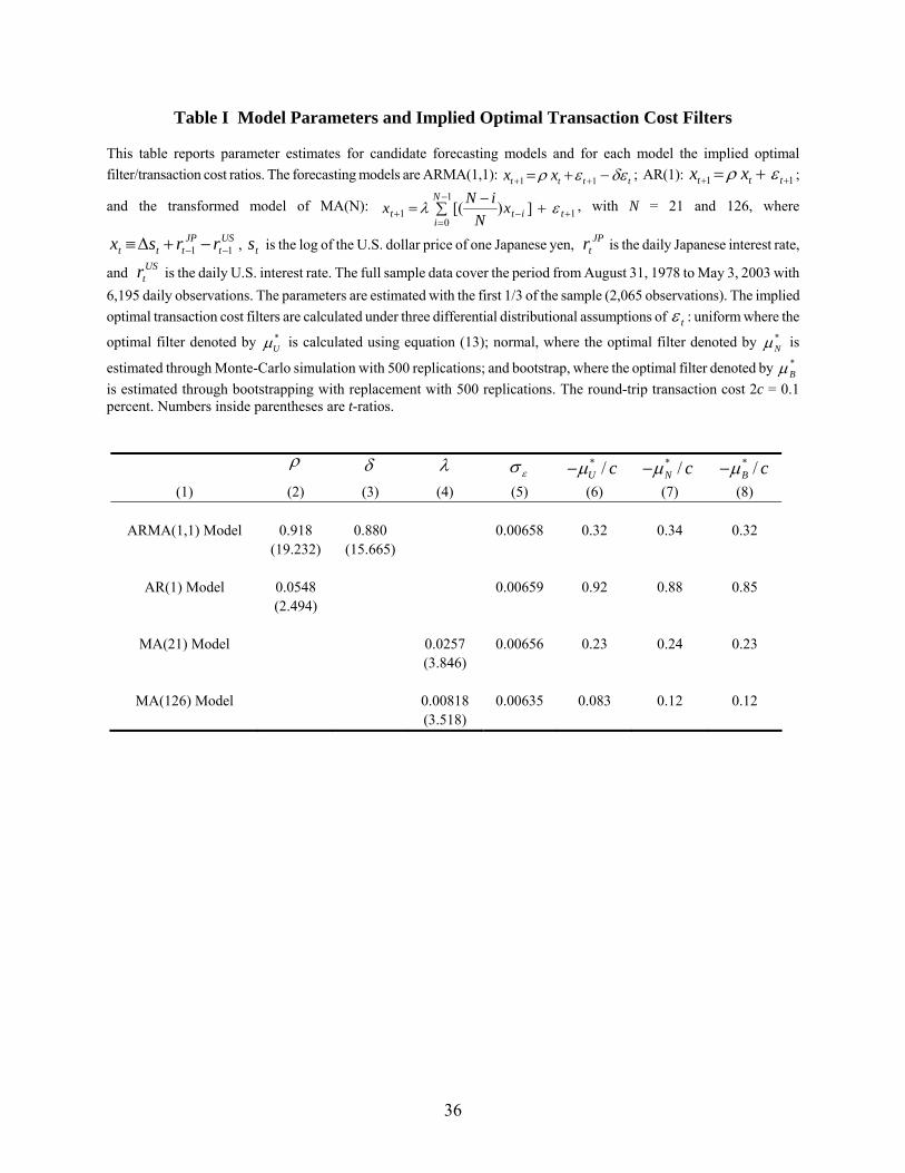
36

Table I Model Parameters and Implied Optimal Transaction Cost Filters This table reports parameter estimates for candidate forecasting models and for each model the implied optimal filter/transaction cost ratios. The forecasting models are ARMA(1,1): tttt xx δεερ −+= ++ 11 ; AR(1): 11 ++ += ttt xx ερ ;

and the transformed model of MA(N): 11

01 ])[( +

−

=−+ +∑

−= t

N

iitt x

NiNx ελ , with N = 21 and 126, where

USt

JPttt rrsx 11 −− −+∆≡ , ts is the log of the U.S. dollar price of one Japanese yen, JP

tr is the daily Japanese interest rate,

and UStr is the daily U.S. interest rate. The full sample data cover the period from August 31, 1978 to May 3, 2003 with

6,195 daily observations. The parameters are estimated with the first 1/3 of the sample (2,065 observations). The implied optimal transaction cost filters are calculated under three differential distributional assumptions of tε : uniform where the

optimal filter denoted by *Uµ is calculated using equation (13); normal, where the optimal filter denoted by *

Nµ is

estimated through Monte-Carlo simulation with 500 replications; and bootstrap, where the optimal filter denoted by *Bµ

is estimated through bootstrapping with replacement with 500 replications. The round-trip transaction cost 2c = 0.1 percent. Numbers inside parentheses are t-ratios.

ρ δ λ εσ * /U cµ− * /N cµ− * /B cµ−

(1) (2) (3) (4) (5) (6) (7) (8)

ARMA(1,1) Model 0.918 0.880 0.00658 0.32 0.34 0.32 (19.232) (15.665)

AR(1) Model 0.0548 0.00659 0.92 0.88 0.85 (2.494)

MA(21) Model 0.0257 0.00656 0.23 0.24 0.23 (3.846)

MA(126) Model 0.00818 0.00635 0.083 0.12 0.12 (3.518)

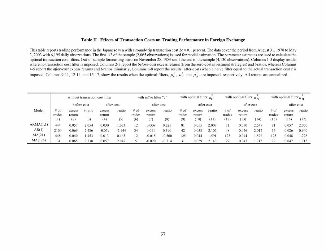
37

Table II Effects of Transaction Costs on Trading Performance in Foreign Exchange

This table reports trading performance in the Japanese yen with a round-trip transaction cost 2c = 0.1 percent. The data cover the period from August 31, 1978 to May 3, 2003 with 6,195 daily observations. The first 1/3 of the sample (2,065 observations) is used for model estimation. The parameter estimates are used to calculate the optimal transaction cost filters. Out-of-sample forecasting starts on November 28, 1986 until the end of the sample (4,130 observations). Columns 1-5 display results where no transaction cost filter is imposed. Columns 2-3 report the before-cost excess returns (from the zero-cost investment strategies) and t-ratios, whereas Columns 4-5 report the after-cost excess returns and t-ratios. Similarly, Columns 6-8 report the results (after-cost) when a naïve filter equal to the actual transaction cost c is imposed. Columns 9-11, 12-14, and 15-17, show the results when the optimal filters, *

Uµ , *Nµ and *

Bµ , are imposed, respectively. All returns are annualized.

without transaction cost filter with naïve filter “c” with optimal filter *Uµ with optimal filter *

Nµ with optimal filter *Bµ

before cost after cost after cost after cost after cost after cost Model # of

trades excess return

t-ratio excess return

t-ratio # of trades

excess return

t-ratio # of trades

excess return

t-ratio # of trades

excess return

t-ratio # of trades

excess return

t-ratio

(1) (2) (3) (4) (5) (6) (7) (8) (9) (10) (11) (12) (13) (14) (15) (16) (17) ARMA(1,1) 444 0.057 2.054 0.030 1.073 12 0.006 0.225 81 0.055 2.007 71 0.070 2.549 81 0.057 2.050

AR(1) 2100 0.069 2.486 -0.059 -2.144 34 0.011 0.390 42 0.058 2.105 48 0.056 2.017 66 0.026 0.940 MA(21) 448 0.040 1.453 0.013 0.463 12 -0.015 -0.560 125 0.044 1.591 123 0.044 1.596 125 0.048 1.728 MA(126) 131 0.065 2.338 0.057 2.047 5 -0.020 -0.714 31 0.059 2.143 29 0.047 1.715 29 0.047 1.715

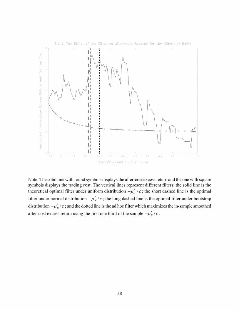
38

Note: The solid line with round symbols displays the after-cost excess return and the one with square symbols displays the trading cost. The vertical lines represent different filters: the solid line is the theoretical optimal filter under uniform distribution * /U cµ− ; the short dashed line is the optimal filter under normal distribution * /N cµ− ; the long dashed line is the optimal filter under bootstrap distribution * /B cµ− ; and the dotted line is the ad hoc filter which maximizes the in-sample smoothed after-cost excess return using the first one third of the sample * /E cµ− .

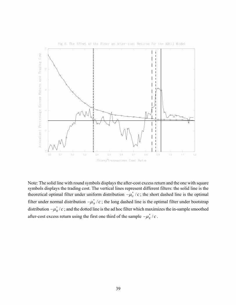
39

Note: The solid line with round symbols displays the after-cost excess return and the one with square symbols displays the trading cost. The vertical lines represent different filters: the solid line is the theoretical optimal filter under uniform distribution * /U cµ− ; the short dashed line is the optimal filter under normal distribution * /N cµ− ; the long dashed line is the optimal filter under bootstrap distribution * /B cµ− ; and the dotted line is the ad hoc filter which maximizes the in-sample smoothed after-cost excess return using the first one third of the sample * /E cµ− .

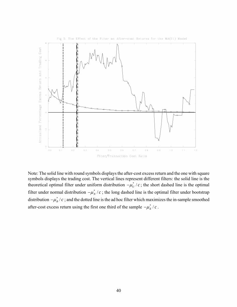
40

Note: The solid line with round symbols displays the after-cost excess return and the one with square symbols displays the trading cost. The vertical lines represent different filters: the solid line is the theoretical optimal filter under uniform distribution * /U cµ− ; the short dashed line is the optimal filter under normal distribution * /N cµ− ; the long dashed line is the optimal filter under bootstrap distribution * /B cµ− ; and the dotted line is the ad hoc filter which maximizes the in-sample smoothed after-cost excess return using the first one third of the sample * /E cµ− .

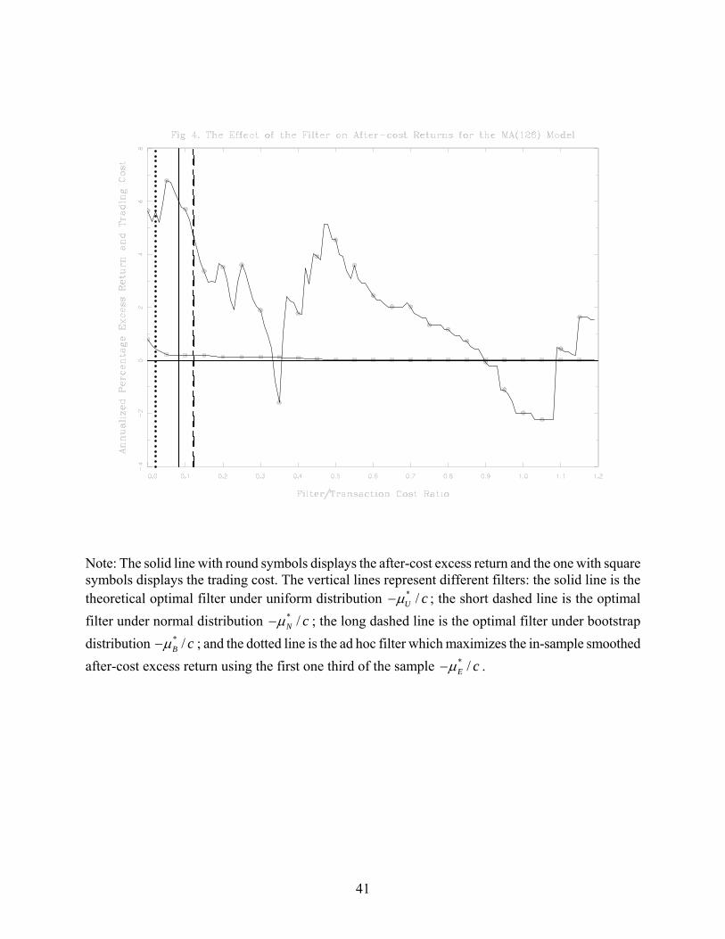
41

Note: The solid line with round symbols displays the after-cost excess return and the one with square symbols displays the trading cost. The vertical lines represent different filters: the solid line is the theoretical optimal filter under uniform distribution * /U cµ− ; the short dashed line is the optimal filter under normal distribution * /N cµ− ; the long dashed line is the optimal filter under bootstrap distribution * /B cµ− ; and the dotted line is the ad hoc filter which maximizes the in-sample smoothed after-cost excess return using the first one third of the sample * /E cµ− .