Loughborough UniversityInstitutional Repository

Optimisation based controlframework for autonomousvehicles: algorithm and

experiment

This item was submitted to Loughborough University's Institutional Repositoryby the/an author.

Citation: LIU, C., CHEN, W-H. and ANDREWS, J., 2010. Optimisationbased control framework for autonomous vehicles: algorithm and experiment.IN: International Conference on Mechatronics and Automation (ICMA), Xi'anChina, 4-7 Aug. 7pp.

Additional Information:

• This is a conference paper [ c© IEEE]. It is also available at:http://ieeexplore.ieee.org/ Personal use of this material is permitted.However, permission to reprint/republish this material for advertising orpromotional purposes or for creating new collective works for resale orredistribution to servers or lists, or to reuse any copyrighted componentof this work in other works must be obtained from the IEEE.

Metadata Record: https://dspace.lboro.ac.uk/2134/7731

Version: Published

Publisher: c© IEEE

Please cite the published version.

This item was submitted to Loughborough’s Institutional Repository (https://dspace.lboro.ac.uk/) by the author and is made available under the

following Creative Commons Licence conditions.

For the full text of this licence, please go to: http://creativecommons.org/licenses/by-nc-nd/2.5/

Optimisation based control framework forautonomous vehicles: algorithm and experiment

Cunjia Liu, Wen-Hua Chen, Senior Member, IEEE, John Andrews

Abstract—This paper addresses both path tracking and localtrajectory generation for autonomous ground vehicles. An opti-misation based two-level control framework is proposed for thistask. The high-level control operates in a receding horizon fashionby taking into account real-time sensory information. It generatesa feasible trajectory satisfying the nonlinear vehicle model andvarious constraints, and resolves possible short term conflictsthrough on-line optimisation. The low-level controller drives thevehicle tracking the local trajectory in the presence of uncertaintyand disturbance. It is shown that the time varying controllerproposed in this paper guarantees stability under all possibletrajectories. The two-level control structure significantly facili-tates the real-time implementation of optimisation based controltechniques on systems with fast dynamics such as autonomousvehicle systems. The proposed technique is implemented on asmall-scale autonomous vehicle in the lab. Both simulation andexperimental results demonstrate the efficiency of the proposedtechnique.

I. INTRODUCTION

Autonomous vehicles, including unmanned aerial vehicles

(UAV) and ground vehicles (UGV), have been drawing a

considerable attention from both industry and academic in the

past two decades, with the expectation of a wide range of

applications. Versatile tasks can be performed by autonomous

vehicles to replace human or human operated vehicles. An

essential function required for an autonomous vehicle perform-

ing a mission is to track reference trajectories or waypoints

either pre-planned beforehand or dynamically generated by

a supervisory layer such as human operators or intelligent

mission planner.

The mission-level planner for autonomous vehicles focuses

on achieving the global goal while minimising risk and oper-

ates at a large time scale. In this setting, the vehicle is usually

treated as a point mass and routines are generated mainly to

maximize the mission success rate by taking into account

the location of targets, threats and geographic information

[1]. Hence trajectories generated by the high-level mission

planner may not fully satisfy vehicle kinematic constraints and

may also need alterations when encountering newly developed

threats or obstacles.

To this end, local trajectory generation and vehicle control

has been studied by many researchers and a number of

methods have been proposed [2]. As all the autonomous

Cunjia Liu and Wen-Hua Chen are with Department of Aeronautical andAutomotive Engineering, Loughborough University, Loughborough, LE113TU, UK. e-mail: {c.liu5, w.chen}@lboro.ac.uk

John Andrews is with Nottingham Transportation Engineering Cen-tre, University of Nottingham, Nottingham, NG7 2RD, UK. e-mail:John.Andrews@nottingham.ac.uk

vehicles are equipped with sensors that can provide local infor-

mation within a certain range, model predictive control (MPC)

provides a promising, natural framework for this problem

since the environment information is changed/updated as the

vehicle proceeds. Both vehicle dynamics and environmental

information can be considered in this approach. Therefore it

is argued that MPC may offer a number of advantages over

other methods [3].

The vehicle under consideration in this paper is a rear-

wheel-driven ground vehicle. The kinematics of such a vehicle

is commonly described by a nonholonomic nonlinear model.

Applications of MPC on nonholonomic mobile robots can be

found in [4], [5]. The corresponding MPC stability issues also

have been discussed in [6], [7]. More recently, a UAV path

following problem has been cast into this category and solved

using MPC, but the obstacle avoidance has not been taken into

account [8].

In MPC setting, an optimisation problem (OP) has to

be solved within each sampling interval. This is the main

obstacle of applying MPC into plants with fast dynamics

such as vehicles. Although a few MPC algorithms in this

field have been implemented in real-time [9], [10], they are

based on linear MPC settings. For nonlinear vehicle models

with obstacles avoidance function, a computationally intensive

nonlinear optimisation problem is involved in calculation of

the control command. Real-time implementation of nonlinear

MPC on autonomous vehicles still poses a major challenge

[11].

This paper proposes an optimisation based control frame-

work which combines MPC with traditional control tech-

niques. Instead of attempting to implement a single non-

linear MPC, the proposed framework employs a two-level

control structure where the high-level controller generates

local trajectories by exploiting both vehicle and environment

information updated by sensors in real-time such as obstacles

and other road users. The vehicle information includes a

nonlinear vehicle model and various constraints such as non-

holonomic constraints and maximum control inputs. The low-

level controller is designed based on the linearisation around

a reference trajectory provided by the high-level controller

to stabilise the vehicle in the presence of disturbances and

uncertainties. These two levels of controller are operated at

different time scales: the high-level on a lower sampling rate,

whereas the low-level on a higher one. Therefore the proposed

optimisation based two-level control framework facilitates

real-time implementation since it can simultaneously cope

with the heavy computational burden demanded by on-line

978-1-4244-5141-8/10/$26.00 © 2010 IEEE 1030

Proceedings of the 2010 IEEEInternational Conference on Mechatronics and Automation

August 4-7, 2010, Xi'an, China

optimisation solvers and fast feedback as required by vehicle

stabilization and control. Moreover, the high-level MPC adopts

a modified formulation to further reduce the computation load

comparing to the early similar works [12].

With the feature of reduced computational requirements

on the real-time implementation, the functions of proposed

control framework include:

• regenerating feasible local trajectories for the vehicles

satisfying various constraints such as nonholonomic con-

straints and maximum control inputs and nonlinear vehi-

cle models;

• resolving short term conflicts with other road users and

obstacles;

• tracking the generated trajectories in the presence of

disturbances and uncertainties with a local controller that

guarantees stability under all possible trajectories.

The rest of this paper is organised as follows. Section II

describes the high-level MPC formulation in a discrete time

setting with an emphasis on the real-time implementation.

The two-level framework including the design of low-level

controller is introduced in Section III. In Section IV the

simulation and experiment results are illustrated to verify the

proposed approach, followed by a conclusion in Section V.

II. MPC FORMULATION

A. Vehicle model

Despite the apparent simplicity of the kinematic model of

a car-like vehicle, the design of controller for this kind of

system can be considered a challenge owing to the existence

of nonholonomic constraints. Basically, the nonholonomic

constraint related to a car-like vehicle refers to the constraint of

rolling without slipping between the rear wheels and ground.

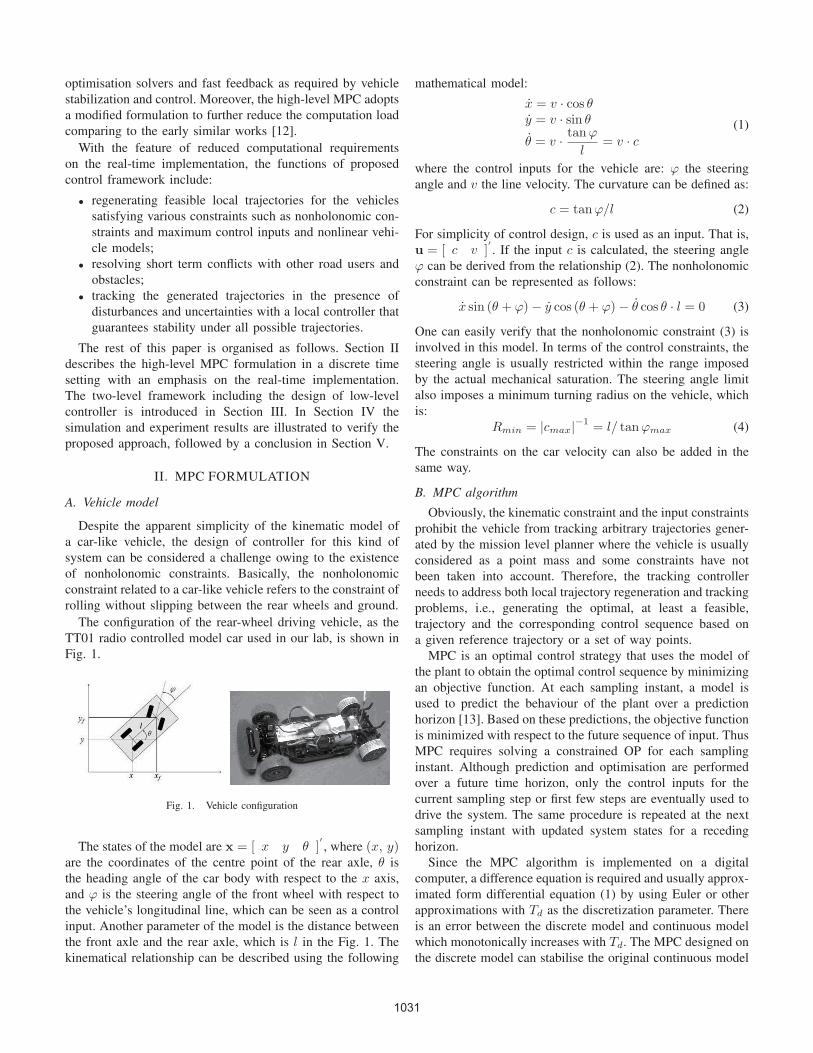
The configuration of the rear-wheel driving vehicle, as the

TT01 radio controlled model car used in our lab, is shown in

Fig. 1.

Fig. 1. Vehicle configuration

The states of the model are x = [ x y θ ]′, where (x, y)

are the coordinates of the centre point of the rear axle, θ is

the heading angle of the car body with respect to the x axis,

and ϕ is the steering angle of the front wheel with respect to

the vehicle’s longitudinal line, which can be seen as a control

input. Another parameter of the model is the distance between

the front axle and the rear axle, which is l in the Fig. 1. The

kinematical relationship can be described using the following

mathematical model:

x = v · cos θy = v · sin θ

θ = v · tanϕ

l= v · c

(1)

where the control inputs for the vehicle are: ϕ the steering

angle and v the line velocity. The curvature can be defined as:

c = tanϕ/l (2)

For simplicity of control design, c is used as an input. That is,

u = [ c v ]′. If the input c is calculated, the steering angle

ϕ can be derived from the relationship (2). The nonholonomic

constraint can be represented as follows:

x sin (θ + ϕ) − y cos (θ + ϕ) − θ cos θ · l = 0 (3)

One can easily verify that the nonholonomic constraint (3) is

involved in this model. In terms of the control constraints, the

steering angle is usually restricted within the range imposed

by the actual mechanical saturation. The steering angle limit

also imposes a minimum turning radius on the vehicle, which

is:

Rmin = |cmax|−1 = l/ tanϕmax (4)

The constraints on the car velocity can also be added in the

same way.

B. MPC algorithm

Obviously, the kinematic constraint and the input constraints

prohibit the vehicle from tracking arbitrary trajectories gener-

ated by the mission level planner where the vehicle is usually

considered as a point mass and some constraints have not

been taken into account. Therefore, the tracking controller

needs to address both local trajectory regeneration and tracking

problems, i.e., generating the optimal, at least a feasible,

trajectory and the corresponding control sequence based on

a given reference trajectory or a set of way points.

MPC is an optimal control strategy that uses the model of

the plant to obtain the optimal control sequence by minimizing

an objective function. At each sampling instant, a model is

used to predict the behaviour of the plant over a prediction

horizon [13]. Based on these predictions, the objective function

is minimized with respect to the future sequence of input. Thus

MPC requires solving a constrained OP for each sampling

instant. Although prediction and optimisation are performed

over a future time horizon, only the control inputs for the

current sampling step or first few steps are eventually used to

drive the system. The same procedure is repeated at the next

sampling instant with updated system states for a receding

horizon.

Since the MPC algorithm is implemented on a digital

computer, a difference equation is required and usually approx-

imated form differential equation (1) by using Euler or other

approximations with Td as the discretization parameter. There

is an error between the discrete model and continuous model

which monotonically increases with Td. The MPC designed on

the discrete model can stabilise the original continuous model

1031

if Td is small enough [14]. However, the small Td increases

the computational burden as there are more control variables

to be decided within the same prediction duration. If solving

OP cannot be completed in such a time interval, MPC cannot

be implemented in real-time. This is particularly important for

safety critical systems with fast dynamics such as autonomous

vehicles.

To avoid this problem, this paper introduces another impor-

tant parameter, namely the MPC sampling time Ts, defined

as the interval of the MPC updating the current states and

generating the new control sequence. In the conventional MPC

setting, Td = Ts. However, with respect to Td and Ts we

define the control holding horizon N , which indicates the

control inputs keeping the constant values for N integration

steps. These three parameters have to satisfy the relationship:

Ts = N · Td. With the modified time setting the time allowed

for OP solving is increased to Ts, while maintaining the

resolution of the integration to Td in the prediction. Note that

although other MPC formulations may also have the different

sampling time like Ts and Td [8], [12], they did not use the

control holding mechanism.

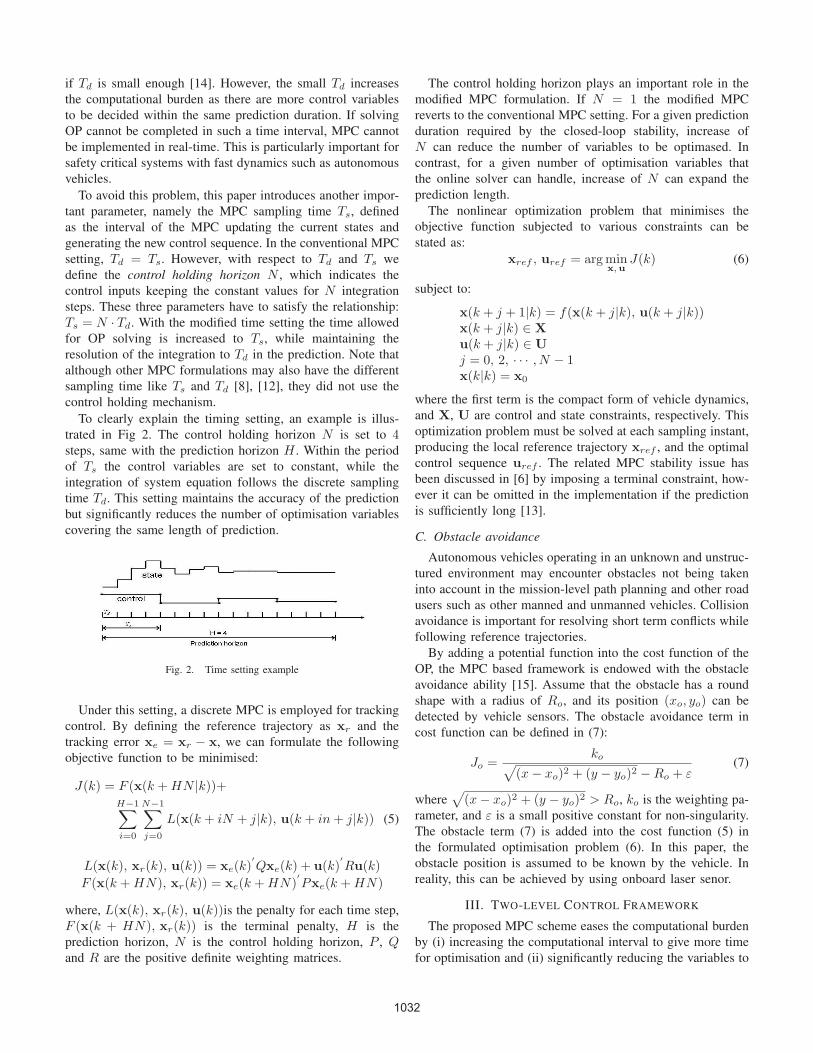
To clearly explain the timing setting, an example is illus-

trated in Fig 2. The control holding horizon N is set to 4steps, same with the prediction horizon H . Within the period

of Ts the control variables are set to constant, while the

integration of system equation follows the discrete sampling

time Td. This setting maintains the accuracy of the prediction

but significantly reduces the number of optimisation variables

covering the same length of prediction.

Fig. 2. Time setting example

Under this setting, a discrete MPC is employed for tracking

control. By defining the reference trajectory as xr and the

tracking error xe = xr − x, we can formulate the following

objective function to be minimised:

J(k) = F (x(k + HN |k))+H−1∑i=0

N−1∑j=0

L(x(k + iN + j|k), u(k + in + j|k)) (5)

L(x(k), xr(k), u(k)) = xe(k)′Qxe(k) + u(k)

′Ru(k)

F (x(k + HN), xr(k)) = xe(k + HN)′Pxe(k + HN)

where, L(x(k), xr(k), u(k))is the penalty for each time step,

F (x(k + HN), xr(k)) is the terminal penalty, H is the

prediction horizon, N is the control holding horizon, P , Qand R are the positive definite weighting matrices.

The control holding horizon plays an important role in the

modified MPC formulation. If N = 1 the modified MPC

reverts to the conventional MPC setting. For a given prediction

duration required by the closed-loop stability, increase of

N can reduce the number of variables to be optimased. In

contrast, for a given number of optimisation variables that

the online solver can handle, increase of N can expand the

prediction length.

The nonlinear optimization problem that minimises the

objective function subjected to various constraints can be

stated as:

xref , uref = arg minx, u

J(k) (6)

subject to:

x(k + j + 1|k) = f(x(k + j|k), u(k + j|k))x(k + j|k) ∈ Xu(k + j|k) ∈ Uj = 0, 2, · · · , N − 1x(k|k) = x0

where the first term is the compact form of vehicle dynamics,

and X, U are control and state constraints, respectively. This

optimization problem must be solved at each sampling instant,

producing the local reference trajectory xref , and the optimal

control sequence uref . The related MPC stability issue has

been discussed in [6] by imposing a terminal constraint, how-

ever it can be omitted in the implementation if the prediction

is sufficiently long [13].

C. Obstacle avoidance

Autonomous vehicles operating in an unknown and unstruc-

tured environment may encounter obstacles not being taken

into account in the mission-level path planning and other road

users such as other manned and unmanned vehicles. Collision

avoidance is important for resolving short term conflicts while

following reference trajectories.

By adding a potential function into the cost function of the

OP, the MPC based framework is endowed with the obstacle

avoidance ability [15]. Assume that the obstacle has a round

shape with a radius of Ro, and its position (xo, yo) can be

detected by vehicle sensors. The obstacle avoidance term in

cost function can be defined in (7):

Jo =ko√

(x − xo)2 + (y − yo)2 − Ro + ε(7)

where√

(x − xo)2 + (y − yo)2 > Ro, ko is the weighting pa-

rameter, and ε is a small positive constant for non-singularity.

The obstacle term (7) is added into the cost function (5) in

the formulated optimisation problem (6). In this paper, the

obstacle position is assumed to be known by the vehicle. In

reality, this can be achieved by using onboard laser senor.

III. TWO-LEVEL CONTROL FRAMEWORK

The proposed MPC scheme eases the computational burden

by (i) increasing the computational interval to give more time

for optimisation and (ii) significantly reducing the variables to

1032

be optimised. However, the MPC strategy becomes an open-

loop optimal control within the interval Ts. Unfortunately, due

to the mismatch between the mathematical model and the real

plant, the noises and disturbances in the process, this kind of

optimal control would not perform as being designed. Within

the interval Ts, the MPC cannot suppress any tracking error.

The bandwidth associated with the MPC is not adequate for

stabilising and control the vehicles that have fast dynamics.

In order to avoid these difficulties in the MPC, a two-

level structure is adopted in the control framework. The high-

level controller is the discrete MPC strategy described before,

which can provide optimised reference trajectory and the

corresponding control inputs, whereas the low-level controller

is a conventional feedback controller that can track the local

trajectories and provide stability around the trajectory in the

presence of disturbances and uncertainties. The high-level con-

troller runs at a lower sampling rate Ts to adapt the calculation

time caused by solving the nonlinear optimisation problem.

In contrast, the low-level controller works at a much higher

sampling rate to stabilise the plant. The control structure is

shown in Fig 3.

Fig. 3. Two-level control framework

In the implementation, the high-level MPC provides optimal

local trajectories and also the corresponding optimal control

inputs. The low-level controller measures current states and

then compares them with the high-level state reference. The

error signals are used to generate compensation control efforts

through the local controller. The overall control inputs applied

to the vehicle consist of two parts: the reference control inputs

and the compensation control generated by the local controller.

The low-level controller can be designed based on perturba-

tion models around the reference state produced by high-level

MPC. Since the low-level control works in a much higher

sampling rate, the controller design can be performed in the

continuous time domain. The vehicle model (1) can be lin-

earised around the trajectory and nominal inputs (xref ,uref )as following:

x = f(x, u) ≈ f(xref , uref ) +∂f

∂x

∣∣∣∣xref

(x − xref )

+∂f

∂u

∣∣∣∣uref

(u − uref ) (8)

By defining the error state Δx = x − xref and control

compensation Δu = u−uref . The error system can be stated

as:

Δx =∂f

∂x

∣∣∣∣xref

Δx +∂f

∂u

∣∣∣∣uref

Δu = AΔx + BΔu (9)

where

A =

⎡⎣0 0 −vref · sin θref

0 0 vref · cos θref

0 0 0

⎤⎦B =

⎡⎣ 0 cos θref

0 sin θref

vref cref

⎤⎦ .

In terms of the time varying system (9), a time varying

feedback law is proposed as in (10):

K =[ −k1 sin θref k1 cos θref k2

k3vref cos θref k3vref sin θref 0

](10)

where k1, k2 and k3 are control parameters to be tuned, the

other parameters depend on the high-level reference. Then the

state transition matrix of the closed-loop error system Δx =(A − BK)Δx is derived in (11):

v ·⎡⎣ −k3 cos2 θ −k3 cos θ sin θ − sin θ

−k3 cos θ sin θ −k3 sin2 θ cos θk1 sin θ − ck3 cos θ −k1 cos θ − ck3 sin θ −k2

⎤⎦

(11)

For the sake of simplicity, the subscripts for the reference

states are omitted. Since the resulting close-loop system is a

linear time-varying system, the stability can be analysed by

using Lyapunov theory.

By defining the Lyapunov function as (12), and invoking

the closed-loop system (11), the derivative of the Lyapunov

function is derived in (13).

V (Δx) = 0.5(Δx2 + Δy2 + Δθ2) (12)

V = −v · k3(Δxcosθ + Δysinθ)2 − v · k2Δθ2

− vc · k3(Δxcosθ + Δysinθ)Δθ

v · (1 − k1)(−Δxsinθ + Δycosθ)Δθ (13)

By defining the tracking error in the vehicle body coordi-

nates: Δxb = Δxcosθ+Δysinθ, Δyb = −Δxsinθ+Δycosθand Δθb = Δθ, the equation (13) is equivalent to (14).

V = − vk3(Δxb − c

2Δθ)2 − v(k2 − c2

2k3)Δθ2

− v(k1 − 1)ΔybΔθb (14)

To guarantee the stability of closed-loop, i.e. V < 0, the

design of low-level control parameters has to follow the rules

in (15):

k3 > 0 (15a)

k2 >c2max

2k3 (15b)

(k1 − 1)sign(ΔybΔθb) > 0 (15c)

1033

IV. SIMULATION AND EXPERIMENT

A. Numerical simulation

To show the performance of the MPC strategy, simulation

was firstly carried out based on the Subaru TT01 model car

in the lab. After various driving tests in the lab, the model of

the vehicle has been built. Simulation for a number of tasks

has been performed.

One simulation task is to track an eight-shaped trajectory

with obstacles. In the simulation, the matrices Q and R in

the cost function of MPC are chosen as diag(1, 1, 0.5) and

diag(0.1, 0.1) respectively. The terminal penalty weighting

P is chosen as diag(10, 10, 5). The discretization time of

model Td is 0.1s and the MPC sampling time Ts is set to

0.5s which means control holding horizon N is 5 steps. The

prediction horizon H is set to 6 steps, suggesting that the

overall prediction duration is 3 seconds. In terms of input

constraints, the steering angle ϕ is limited from −0.4rad to

0.4rad and the line speed v from 0.15m/s to 0.8m/s. The

low-level control parameters are k1 = 1 ± 0.5 depending on

sign(ΔybΔθb), k2 = 2.5 and k3 = 1.

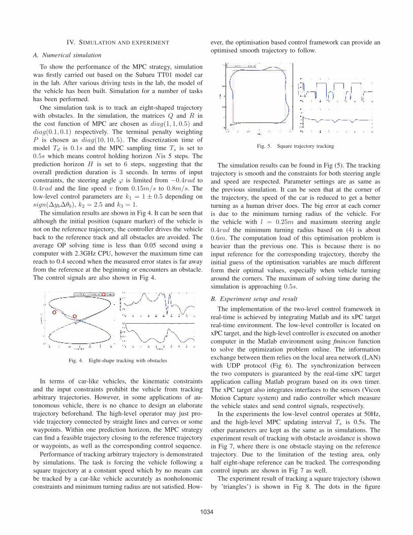
The simulation results are shown in Fig 4. It can be seen that

although the initial position (square marker) of the vehicle is

not on the reference trajectory, the controller drives the vehicle

back to the reference track and all obstacles are avoided. The

average OP solving time is less than 0.05 second using a

computer with 2.3GHz CPU, however the maximum time can

reach to 0.4 second when the measured error states is far away

from the reference at the beginning or encounters an obstacle.

The control signals are also shown in Fig 4.

Fig. 4. Eight-shape tracking with obstacles

In terms of car-like vehicles, the kinematic constraints

and the input constraints prohibit the vehicle from tracking

arbitrary trajectories. However, in some applications of au-

tonomous vehicle, there is no chance to design an elaborate

trajectory beforehand. The high-level operator may just pro-

vide trajectory connected by straight lines and curves or some

waypoints. Within one prediction horizon, the MPC strategy

can find a feasible trajectory closing to the reference trajectory

or waypoints, as well as the corresponding control sequence.

Performance of tracking arbitrary trajectory is demonstrated

by simulations. The task is forcing the vehicle following a

square trajectory at a constant speed which by no means can

be tracked by a car-like vehicle accurately as nonholonomic

constraints and minimum turning radius are not satisfied. How-

ever, the optimisation based control framework can provide an

optimised smooth trajectory to follow.

Fig. 5. Square trajectory tracking

The simulation results can be found in Fig (5). The tracking

trajectory is smooth and the constraints for both steering angle

and speed are respected. Parameter settings are as same as

the previous simulation. It can be seen that at the corner of

the trajectory, the speed of the car is reduced to get a better

turning as a human driver does. The big error at each corner

is due to the minimum turning radius of the vehicle. For

the vehicle with l = 0.25m and maximum steering angle

0.4rad the minimum turning radius based on (4) is about

0.6m. The computation load of this optimisation problem is

heavier than the previous one. This is because there is no

input reference for the corresponding trajectory, thereby the

initial guess of the optimisation variables are much different

form their optimal values, especially when vehicle turning

around the corners. The maximum of solving time during the

simulation is approaching 0.5s.

B. Experiment setup and result

The implementation of the two-level control framework in

real-time is achieved by integrating Matlab and its xPC target

real-time environment. The low-level controller is located on

xPC target, and the high-level controller is executed on another

computer in the Matlab environment using fmincon function

to solve the optimization problem online. The information

exchange between them relies on the local area network (LAN)

with UDP protocol (Fig 6). The synchronization between

the two computers is guaranteed by the real-time xPC target

application calling Matlab program based on its own timer.

The xPC target also integrates interfaces to the sensors (Vicon

Motion Capture system) and radio controller which measure

the vehicle states and send control signals, respectively.

In the experiments the low-level control operates at 50Hz,

and the high-level MPC updating interval Ts is 0.5s. The

other parameters are kept as the same as in simulations. The

experiment result of tracking with obstacle avoidance is shown

in Fig 7, where there is one obstacle staying on the reference

trajectory. Due to the limitation of the testing area, only

half eight-shape reference can be tracked. The corresponding

control inputs are shown in Fig 7 as well.

The experiment result of tracking a square trajectory (shown

by ’triangles’) is shown in Fig 8. The dots in the figure

1034

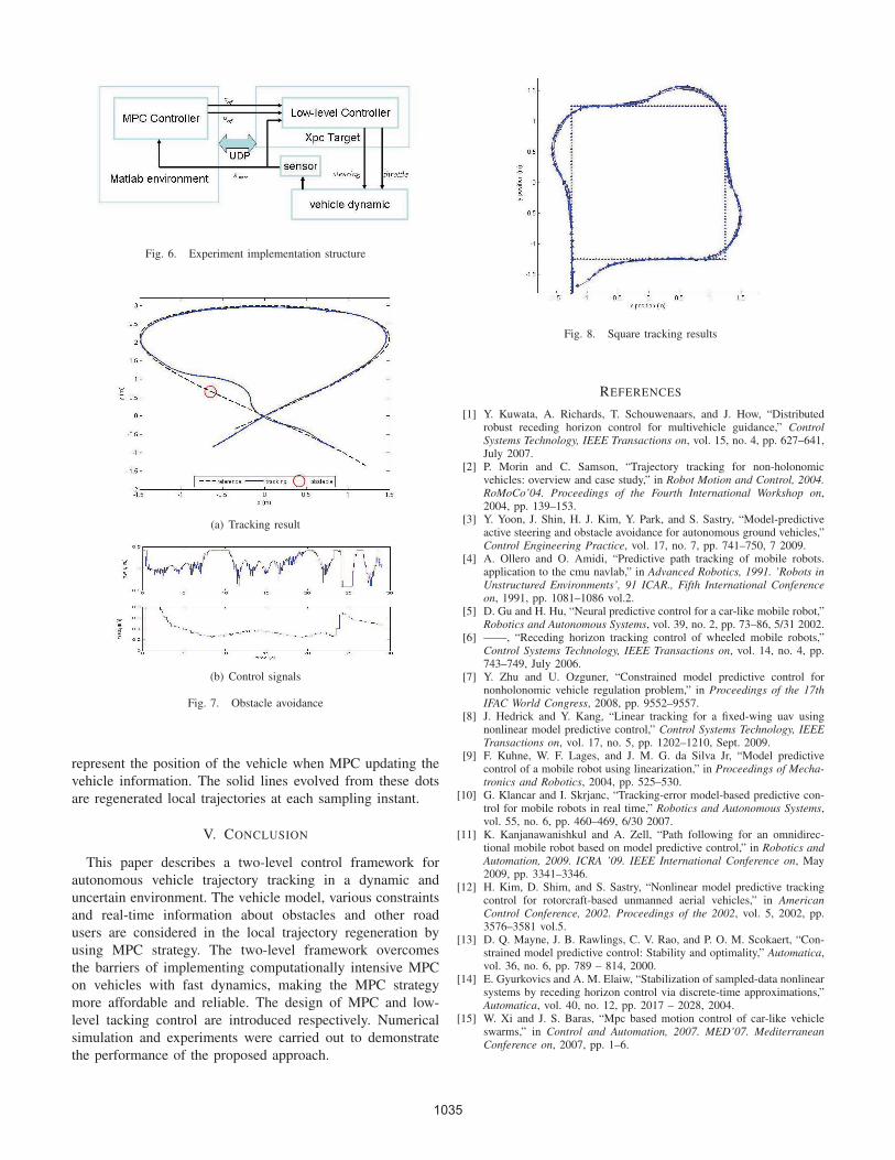
Fig. 6. Experiment implementation structure

(a) Tracking result

(b) Control signals

Fig. 7. Obstacle avoidance

represent the position of the vehicle when MPC updating the

vehicle information. The solid lines evolved from these dots

are regenerated local trajectories at each sampling instant.

V. CONCLUSION

This paper describes a two-level control framework for

autonomous vehicle trajectory tracking in a dynamic and

uncertain environment. The vehicle model, various constraints

and real-time information about obstacles and other road

users are considered in the local trajectory regeneration by

using MPC strategy. The two-level framework overcomes

the barriers of implementing computationally intensive MPC

on vehicles with fast dynamics, making the MPC strategy

more affordable and reliable. The design of MPC and low-

level tacking control are introduced respectively. Numerical

simulation and experiments were carried out to demonstrate

the performance of the proposed approach.

Fig. 8. Square tracking results

REFERENCES

[1] Y. Kuwata, A. Richards, T. Schouwenaars, and J. How, “Distributedrobust receding horizon control for multivehicle guidance,” ControlSystems Technology, IEEE Transactions on, vol. 15, no. 4, pp. 627–641,July 2007.

[2] P. Morin and C. Samson, “Trajectory tracking for non-holonomicvehicles: overview and case study,” in Robot Motion and Control, 2004.RoMoCo’04. Proceedings of the Fourth International Workshop on,2004, pp. 139–153.

[3] Y. Yoon, J. Shin, H. J. Kim, Y. Park, and S. Sastry, “Model-predictiveactive steering and obstacle avoidance for autonomous ground vehicles,”Control Engineering Practice, vol. 17, no. 7, pp. 741–750, 7 2009.

[4] A. Ollero and O. Amidi, “Predictive path tracking of mobile robots.application to the cmu navlab,” in Advanced Robotics, 1991. ’Robots inUnstructured Environments’, 91 ICAR., Fifth International Conferenceon, 1991, pp. 1081–1086 vol.2.

[5] D. Gu and H. Hu, “Neural predictive control for a car-like mobile robot,”Robotics and Autonomous Systems, vol. 39, no. 2, pp. 73–86, 5/31 2002.

[6] ——, “Receding horizon tracking control of wheeled mobile robots,”Control Systems Technology, IEEE Transactions on, vol. 14, no. 4, pp.743–749, July 2006.

[7] Y. Zhu and U. Ozguner, “Constrained model predictive control fornonholonomic vehicle regulation problem,” in Proceedings of the 17thIFAC World Congress, 2008, pp. 9552–9557.

[8] J. Hedrick and Y. Kang, “Linear tracking for a fixed-wing uav usingnonlinear model predictive control,” Control Systems Technology, IEEETransactions on, vol. 17, no. 5, pp. 1202–1210, Sept. 2009.

[9] F. Kuhne, W. F. Lages, and J. M. G. da Silva Jr, “Model predictivecontrol of a mobile robot using linearization,” in Proceedings of Mecha-tronics and Robotics, 2004, pp. 525–530.

[10] G. Klancar and I. Skrjanc, “Tracking-error model-based predictive con-trol for mobile robots in real time,” Robotics and Autonomous Systems,vol. 55, no. 6, pp. 460–469, 6/30 2007.

[11] K. Kanjanawanishkul and A. Zell, “Path following for an omnidirec-tional mobile robot based on model predictive control,” in Robotics andAutomation, 2009. ICRA ’09. IEEE International Conference on, May2009, pp. 3341–3346.

[12] H. Kim, D. Shim, and S. Sastry, “Nonlinear model predictive trackingcontrol for rotorcraft-based unmanned aerial vehicles,” in AmericanControl Conference, 2002. Proceedings of the 2002, vol. 5, 2002, pp.3576–3581 vol.5.

[13] D. Q. Mayne, J. B. Rawlings, C. V. Rao, and P. O. M. Scokaert, “Con-strained model predictive control: Stability and optimality,” Automatica,vol. 36, no. 6, pp. 789 – 814, 2000.

[14] E. Gyurkovics and A. M. Elaiw, “Stabilization of sampled-data nonlinearsystems by receding horizon control via discrete-time approximations,”Automatica, vol. 40, no. 12, pp. 2017 – 2028, 2004.

[15] W. Xi and J. S. Baras, “Mpc based motion control of car-like vehicleswarms,” in Control and Automation, 2007. MED’07. MediterraneanConference on, 2007, pp. 1–6.

1035