optimization 3 - gauss · 3.1.4 polak-ribiere-type conjugate gradient ... if you are unfamiliar...

Optimization 3.1for GAUSSTM

Aptech Systems, Inc.

Information in this document is subject to change without notice and does notrepresent a commitment on the part of Aptech Systems, Inc. The softwaredescribed in this document is furnished under a license agreement or nondis-closure agreement. The software may be used or copied only in accordancewith the terms of the agreement. The purchaser may make one copy of thesoftware for backup purposes. No part of this manual may be reproduced ortransmitted in any form or by any means, electronic or mechanical, includ-ing photocopying and recording, for any purpose other than the purchaser’spersonal use without the written permission of Aptech Systems, Inc.

c©Copyright Aptech Systems, Inc. Black Diamond WA 1984-2010All Rights Reserved.

GAUSS, GAUSS Engine and GAUSS Light are trademarks of AptechSystems, Inc. Other trademarks are the property of their respective owners.

Part Number: 000044Version 3.1Documentation Revision: 1945 April 1, 2011

Contents

Contents

1 Installation

1.1 UNIX/Linux/Mac . . . . . . . . . . . . . . . . . . . . . . . . . . . . . . 1-11.1.1 Download . . . . . . . . . . . . . . . . . . . . . . . . . . . . 1-11.1.2 CD . . . . . . . . . . . . . . . . . . . . . . . . . . . . . . . . 1-2

1.2 Windows . . . . . . . . . . . . . . . . . . . . . . . . . . . . . . . . . . 1-21.2.1 Download . . . . . . . . . . . . . . . . . . . . . . . . . . . . 1-21.2.2 CD . . . . . . . . . . . . . . . . . . . . . . . . . . . . . . . . 1-21.2.3 64-Bit Windows . . . . . . . . . . . . . . . . . . . . . . . . . 1-3

1.3 Difference Between the UNIX and Windows Versions . . . . . . . . . . 1-3

2 Getting Started

2.0.1 README Files . . . . . . . . . . . . . . . . . . . . . . . . . . 2-12.0.2 Setup . . . . . . . . . . . . . . . . . . . . . . . . . . . . . . . 2-2

3 Optimization

3.1 Algorithms . . . . . . . . . . . . . . . . . . . . . . . . . . . . . . . . . 3-13.1.1 The Steepest Descent Method (STEEP) . . . . . . . . . . . . 3-43.1.2 Newton’s Method (NEWTON) . . . . . . . . . . . . . . . . . . 3-53.1.3 Secant Methods (BFGS, DFP, scaled BFGS) . . . . . . . . . 3-53.1.4 Polak-Ribiere-type Conjugate Gradient (PRCG) . . . . . . . . 3-6

3.2 Line Search . . . . . . . . . . . . . . . . . . . . . . . . . . . . . . . . 3-73.2.1 STEPBT . . . . . . . . . . . . . . . . . . . . . . . . . . . . . 3-73.2.2 BRENT . . . . . . . . . . . . . . . . . . . . . . . . . . . . . . 3-83.2.3 HALF . . . . . . . . . . . . . . . . . . . . . . . . . . . . . . . 3-83.2.4 Random Search . . . . . . . . . . . . . . . . . . . . . . . . . 3-8

3.3 Calling OPTMUM Recursively . . . . . . . . . . . . . . . . . . . . . . . 3-9

iii

Optimization 3.1 for GAUSS

3.4 Using OPTMUM Directly . . . . . . . . . . . . . . . . . . . . . . . . . 3-93.5 Hints on Optimization . . . . . . . . . . . . . . . . . . . . . . . . . . . 3-10

3.5.1 Scaling . . . . . . . . . . . . . . . . . . . . . . . . . . . . . . 3-103.5.2 Condition . . . . . . . . . . . . . . . . . . . . . . . . . . . . . 3-103.5.3 Starting Point . . . . . . . . . . . . . . . . . . . . . . . . . . 3-113.5.4 Managing the Algorithms and Step Length Methods . . . . . . 3-113.5.5 Managing the Computation of the Hessian . . . . . . . . . . . 3-123.5.6 Diagnosis . . . . . . . . . . . . . . . . . . . . . . . . . . . . 3-13

3.6 Function . . . . . . . . . . . . . . . . . . . . . . . . . . . . . . . . . . 3-143.7 Gradient . . . . . . . . . . . . . . . . . . . . . . . . . . . . . . . . . . 3-14

3.7.1 User-Supplied Analytical Gradient . . . . . . . . . . . . . . . 3-143.7.2 User-Supplied Numerical Gradient . . . . . . . . . . . . . . . 3-15

3.8 Hessian . . . . . . . . . . . . . . . . . . . . . . . . . . . . . . . . . . . 3-173.8.1 User-Supplied Analytical Hessian . . . . . . . . . . . . . . . . 3-173.8.2 User-Supplied Numerical Hessian . . . . . . . . . . . . . . . 3-17

3.9 Run-Time Switches . . . . . . . . . . . . . . . . . . . . . . . . . . . . 3-183.10 Error Handling . . . . . . . . . . . . . . . . . . . . . . . . . . . . . . . 3-19

3.10.1 Return Codes . . . . . . . . . . . . . . . . . . . . . . . . . . 3-193.10.2 Error Trapping . . . . . . . . . . . . . . . . . . . . . . . . . . 3-20

3.11 Example . . . . . . . . . . . . . . . . . . . . . . . . . . . . . . . . . . 3-213.12 References . . . . . . . . . . . . . . . . . . . . . . . . . . . . . . . . . 3-22

4 Optimization Reference

optmum . . . . . . . . . . . . . . . . . . . . . . . . . . . . . . . . . . . . . . 4-1optset . . . . . . . . . . . . . . . . . . . . . . . . . . . . . . . . . . . . . . . 4-9optprt . . . . . . . . . . . . . . . . . . . . . . . . . . . . . . . . . . . . . . . 4-10gradfd . . . . . . . . . . . . . . . . . . . . . . . . . . . . . . . . . . . . . . . 4-11gradcd . . . . . . . . . . . . . . . . . . . . . . . . . . . . . . . . . . . . . . . 4-13gradre . . . . . . . . . . . . . . . . . . . . . . . . . . . . . . . . . . . . . . . 4-15

iv

Contents

Index

v

Installation

Installation 11.1 UNIX/Linux/Mac

If you are unfamiliar with UNIX/Linux/Mac, see your system administrator or systemdocumentation for information on the system commands referred to below.

1.1.1 Download

1. Copy the .tar.gz or .zip file to /tmp.

2. If the file has a .tar.gz extension, unzip it using gunzip. Otherwise skip to step 3.

gunzip app_appname_vernum.revnum_UNIX.tar.gz

3. cd to your GAUSS or GAUSS Engine installation directory. We are assuming/usr/local/gauss in this case.

cd /usr/local/gauss

1-1


4. Use tar or unzip, depending on the file name extension, to extract the file.

tar xvf /tmp/app_appname_vernum.revnum_UNIX.tar– or –unzip /tmp/app_appname_vernum.revnum_UNIX.zip

1.1.2 CD

1. Insert the Apps CD into your machine’s CD-ROM drive.

2. Open a terminal window.

3. cd to your current GAUSS or GAUSS Engine installation directory. We areassuming /usr/local/gauss in this case.

cd /usr/local/gauss

4. Use tar or unzip, depending on the file name extensions, to extract the files foundon the CD. For example:

tar xvf /cdrom/apps/app_appname_vernum.revnum_UNIX.tar– or –unzip /cdrom/apps/app_appname_vernum.revnum_UNIX.zip

However, note that the paths may be different on your machine.

1.2 Windows

1.2.1 Download

Unzip the .zip file into your GAUSS or GAUSS Engine installation directory.

1.2.2 CD

1. Insert the Apps CD into your machine’s CD-ROM drive.

1-2

Installation

Installation

2. Unzip the .zip files found on the CD to your GAUSS or GAUSS Engineinstallation directory.

1.2.3 64-Bit Windows

If you have both the 64-bit version of GAUSS and the 32-bit Companion Edition installedon your machine, you need to install any GAUSS applications you own in both GAUSSinstallation directories.

1.3 Difference Between the UNIX and Windows Versions

• If the functions can be controlled during execution by entering keystrokes from thekeyboard, it may be necessary to press ENTER after the keystroke in the UNIXversion.

1-3

Getting

Started

Getting Started 2GAUSS 3.1.0+ is required to use these routines. See _rtl_ver in src/gauss.dec.

The Optimization version number is stored in a global variable:

_optmum_ver 3×1 matrix, the first element contains the major version number, thesecond element the minor version number, and the third element the revisionnumber.

If you call for technical support, you may be asked for the version of your copy ofOptimization.

2.0.1 README Files

If there is a README.opt file, it contains any last minute information on the Optimizationprocedures. Please read it before using them.

2-1


2.0.2 Setup

In order to use the procedures in the Optimization or OPTMUM Module, theOPTMUM library must be active. This is done by including optmum in the librarystatement at the top of your program or command file:

library optmum,pgraph;

2-2

Optim

ization

Optimization 3written by

Ronald Schoenberg

This module contains the procedure OPTMUM, which solves the problem:

minimize: f (x)

where f : Rn → R. It is assumed that f has first and second derivatives.

3.1 Algorithms

OPTMUM is a procedure for the minimization of a user-provided function with respect toparameters. It is assumed that the derivatives with respect to the parameters exist and are

3-1


continuous. If the procedures to compute the derivatives analytically are not supplied bythe user, OPTMUM calls procedures to compute them numerically. The user is requiredto supply a procedure for computing the function.

Six algorithms are available in OPTMUM for minimization. These algorithms, as well asthe step length methods, may be modified during execution of OPTMUM.

OPTMUM minimizes functions iteratively and requires initial values for the unknowncoefficients for the first iteration. At each iteration a direction, d, which is a NP×1 vectorwhere NP is the number of coefficients, and a step length, α, are computed.

Direction

The direction, d, is a vector of quantities to be added to the present estimate of thecoefficients. Intuitively, the term refers to the fact that these quantities measure where thecoefficients are going in this iteration. It is computed as the solution to the equation

Hd = −g

where g is an NP×1 gradient vector, that is, a vector of the first derivatives of the functionwith respect to the coefficients, and where H is an NP×NP symmetric matrix H.

Commonly, as well as in previous versions of OPTMUM, the direction is computed as

d = H−1g

Directly inverting H, however, is a numerically risky procedure, and the present version ofOPTMUM avoids inverting matrices altogether. Instead a solve function is called whichresults in greater numerical stability and accuracy.

H is calculated in different ways depending on the type of algorithm selected by the user,or it can be set to a conformable identity matrix. For best results H should be proportional

3-2

Optim

ization

Optimization

to the matrix of the second derivatives of the function with respect to pairs of thecoefficients, i.e., the Hessian matrix, or an estimate of the Hessian.

The Newton Algorithm

In this method H is the Hessian:

H =∂ f∂x∂xt

By default H is computed numerically. If a function to compute the Hessian is providedby the user, then that function is called. If the user has provided a function to compute thegradient, then the Hessian is computed as the gradient of the gradient.

After H has been computed

Hd = −g

is solved for d.

The Secant Algorithms

The calculation of the Hessian is generally a very large computational problem. Thesecant methods (sometimes called quasi-Newton methods) were developed to avoid this.Starting with an initial estimate of the Hessian, or a conformable identity matrix, anupdate is calculated that requires far less computation. The update at each iteration addsmore “information” to the estimate of the Hessian, improving its ability to project thedirection of the descent. Thus after several iterations the secant algorithm should donearly as well as the Newton iteration with much less computation.

3-3


Commonly, as well as in the previous versions of OPTMUM, an estimate of the inverseof the Hessian is updated on each iteration. This is a good strategy for reducingcomputation but is less favorable numerically. This version of OPTMUM instead updatesa Cholesky factorization of the estimate of the Hessian (not its inverse). This method hassuperior numerical properties (Gill and Murray, 1972). The direction is then computed byapplying a solve to the factorization and the gradient.

There are two basic types of secant methods, the BFGS (Broyden, Fletcher, Goldfarb, andShanno), and the DFP (Davidon, Fletcher, and Powell). They are both rank two updates,that is, they are analogous to adding two rows of new data to a previously computedmoment matrix. The Cholesky factorizations of the estimate of the Hessian is updatedusing the GAUSS functions CHOLUP and CHOLDN.

For given C, the Cholesky factorizatoin of the estimate of the Hessian,

C′Cd = −g

is solved for d using the GAUSS CHOLSOL function.

3.1.1 The Steepest Descent Method (STEEP)

In the steepest descent method H is set to the identity matrix. This reduces computationaland memory requirements and, if the problem is large, the reduction is considerable. Inregions far from the minimum, it can be more efficient than other descent methods whichhave a tendency to get confused when the starting point is poor. It descends quiteinefficiently, however, compared to the Newton and secant methods when closer to theminimum. For that reason, the default switching method begins with steepest descent andswitches to the BFGS secant method.

3-4

Optim

ization

Optimization

3.1.2 Newton’s Method (NEWTON)

Newton’s method makes the most demands on the model of all the methods. The methodsucceeds only when everything is well behaved. The tradeoff is that the method convergein fewer iterations than other methods. NEWTON uses both the first and secondderivatives and thus the Hessian must be computed on each iteration. If the Hessian isbeing computed numerically, there is likely to be very little gain over DFP or BFGSbecause while the latter may take many more iterations, the total time to converge is less.

The numerically-computed gradient requires NP functions calls where NP is the numberof parameters, and the numerically-computed Hessian requires NP2 function calls. If thenumber of parameters is large, or the function calculation time-consuming, the Newtonmethod becomes prohibitively computationally expensive. The computational expensecan be significantly reduced, however, if you provide a function to compute the gradient.This reduces the calculation of the gradient to one function call. Moreover, for thenumerical calculation of the Hessian, OPTMUM uses the gradient function – in effectcomputing the Hessian as the gradient of the gradient – and thus reduces the number offunction calls to NP for the Hessian.

3.1.3 Secant Methods (BFGS, DFP, scaled BFGS)

BFGS is the method of Broyden, Fletcher, Goldfarb, and Shanno, and DFP is the methodof Davidon, Fletcher, and Powell. These methods are complementary (Luenberger 1984,page 268). BFGS and DFP are like the NEWTON method in that they use both first andsecond derivative information. However, in DFP and BFGS the Hessian is approximated,reducing considerably the computational requirements. Because they do not explicitlycalculate the second derivatives, they are sometimes called quasi-Newton methods. Theuse of an approximation produces gains in two ways: first, it is less sensitive to thecondition of the model and data, and second, it performs better in all ways than theSTEEPEST DESCENT method. While it takes more iterations than NEWTON, it can beexpected to converge in less overall time (unless analytical second derivatives areavailable in which case it might be a toss-up).

3-5


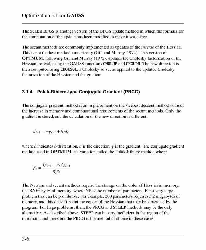
The Scaled BFGS is another version of the BFGS update method in which the formula forthe computation of the update has been modified to make it scale-free.

The secant methods are commonly implemented as updates of the inverse of the Hessian.This is not the best method numerically (Gill and Murray, 1972). This version ofOPTMUM, following Gill and Murray (1972), updates the Cholesky factorization of theHessian instead, using the GAUSS functions CHOLUP and CHOLDN. The new direction isthen computed using CHOLSOL, a Cholesky solve, as applied to the updated Choleskyfactorization of the Hessian and the gradient.

3.1.4 Polak-Ribiere-type Conjugate Gradient (PRCG)

The conjugate gradient method is an improvement on the steepest descent method withoutthe increase in memory and computational requirements of the secant methods. Only thegradient is stored, and the calculation of the new direction is different:

d`+1 = −g`+1 + β`d`

where ` indicates `-th iteration, d is the direction, g is the gradient. The conjugate gradientmethod used in OPTMUM is a variation called the Polak-Ribiere method where

β` =(g`+1 − g`)′g`+1

g′`g`

The Newton and secant methods require the storage on the order of Hessian in memory,i.e., 8NP2 bytes of memory, where NP is the number of parameters. For a very largeproblem this can be prohibitive. For example, 200 parameters requires 3.2 megabytes ofmemory, and this doesn’t count the copies of the Hessian that may be generated by theprogram. For large problems, then, the PRCG and STEEP methods may be the onlyalternative. As described above, STEEP can be very inefficient in the region of theminimum, and therefore the PRCG is the method of choice in these cases.

3-6

Optim

ization

Optimization

3.2 Line Search

Given a direction vector d, the updated estimate of the coefficients is computed

x+ = x + αd

where α is a constant, usually called the step length that increases the descent of thefunction given the direction. OPTMUM includes a variety of methods for computing α.The value of the function to be minimized as a function of α is

F(x + αd)

Given x and d, this is a function of a single variable α. Line search methods attempt tofind a value for α that decreases F. STEPBT is a polynomial fitting method, BRENT andHALF are iterative search methods. A fourth method called ONE forces a step length of 1.

The default line search method is STEPBT. If this or any selected method fails, thenBRENT is tried. If BRENT fails, then HALF is tried. If all of the line search methods fail,then a random search is tried.

3.2.1 STEPBT

STEPBT is an implementation of a similarly named algorithm described in Dennis andSchnabel (1983). It first attempts to fit a quadratic function to F(x + αd) and computes anα that minimizes the quadratic. If that fails it attempts to fit a cubic function. The cubicfunction is more likely to accurately portray the F which is not likely to be very quadraticbut is, however, more costly to compute. STEPBT is the default line search methodbecause it generally produces the best results for the least cost in computational resources.

3-7


3.2.2 BRENT

This method is a variation on the golden section method due to Brent (1972). In thismethod, the function is evaluated at a sequence of test values for α. These test values aredetermined by extrapolation and interpolation using the constant, (

√5 − 1)/2 = .6180....

This constant is the inverse of the so-called “golden ratio” ((√

5 + 1)/2 = 1.6180... and iswhy the method is called a golden section method. This method is generally more efficientthan STEPBT but requires significantly more function evaluations.

3.2.3 HALF

This method first computes F(x + d), i.e., set α = 1. If F(x + d) < F(x) then the steplength is set to 1. If not, then it tries F(x + .5d). The attempted step length is divided byone half each time the function fails to decrease, and exits with the current value when itdoes decrease. This method usually requires the fewest function evaluations (it often onlyrequires one), but it is the least efficient in that it very likely fails to find the step lengththat decreases F the most.

3.2.4 Random Search

If the line search fails, i.e., no α is found such that F(x+αd) < F(x), then a random searchfor a random direction that decreases the function. The radius of the random search isfixed by the global variable, _opmrteps (default = .01), times a measure of the magnitudeof the gradient. OPTMUM makes _opmxtry attempts to find a direction that decreasesthe function, and if all of them fail, the direction with the smallest value for F is selected.

The function should never decrease, but this assumes a well-defined problem. In practice,many functions are not so well-defined, and it often is the case that convergence is morelikely achieved by a direction that puts the function somewhere else on the hyper-surfaceeven if it is at a higher point on the surface. Another reason for permitting an increase inthe function here is that the only alternative is to halt the minimization altogether even

3-8

Optim

ization

Optimization

though it is not at the minimum, and so one might as well retreat to another starting point.If the function repeatedly increases, then you would do well to consider improving eitherthe specification of the problem or the starting point.

3.3 Calling OPTMUM Recursively

The procedure provided by the user for computing the function to be minimized can itselfcall OPTMUM. In fact the number of nested levels is limited only by the amount ofworkspace memory. Each level contains its own set of global variables. Thus nestedcopies can have their own set of attributes and optimization methods.

It is important to call optset for all nested copies, and generally if you wish the outercopy of OPTMUM to retain control over the keyboard, you need to set the global variable_opkey to zero for all the nested copies.

3.4 Using OPTMUM Directly

When OPTMUM is called, it directly references all the necessary globals and passes itsarguments and the values of the globals to a function called _optmum. When _optmumreturns, OPTMUM then sets the output globals to the values returned by _optmum andreturns its arguments directly to the user. _optmum makes no global references to matricesor strings, and all procedures it references have names that begin with an underscore “ ”.

_optmum can be used directly in situations where you do not want any of the globalmatrices and strings in your program. If OPTMUM, optprt and optset are notreferenced, the global matrices and strings in optmum.dec is not included in yourprogram.

The documentation for OPTMUM, the globals it references, and the code itself should besufficient documentation for using _optmum.

3-9


3.5 Hints on Optimization

The critical elements in optimization are scaling, starting point, and the condition of themodel.

When the data are scaled, the starting point reasonably close to the solution, and the dataand model well-conditioned, the iterations converges quickly and without difficulty.

For best results, therefore, you want to prepare the problem so that model iswell-specified, the data scaled, and that a good starting point is available.

3.5.1 Scaling

For best performance the Hessian matrix should be “balanced”, i.e., the sums of thecolumns (or rows) should be roughly equal. In most cases the diagonal elementsdetermined these sums. If some diagonal elements are very large and/or very small withrespect to others, OPTMUM has difficulty converging. How to scale the diagonalelements of the Hessian may not be obvious, but it may suffice to ensure that the constants(or “data”) used in the model are about the same magnitude. 90% of the technical supportcalls complaining about OPTMUM failing to converge are solved by simply scaling theproblem.

3.5.2 Condition

The specification of the model can be measured by the condition of the Hessian. Thesolution of the problem is found by searching for parameter values for which the gradientis zero. If, however, the gradient of the gradient (i.e., the Hessian) is very small for aparticular parameter, then OPTMUM has difficulty deciding on the optimal value since alarge region of the function appears virtually flat to OPTMUM. When the Hessian hasvery small elements the inverse of the Hessian has very large elements and the searchdirection gets buried in the large numbers.

3-10

Optim

ization

Optimization

Poor condition can be caused by bad scaling. It can also be caused by a poor specificationof the model or by bad data. Bad model and bad data are two sides of the same coin. If theproblem is highly nonlinear, it is important that data be available to describe the featuresof the curve described by each of the parameters. For example, one of the parameters ofthe Weibull function describes the shape of the curve as it approaches the upperasymptote. If data are not available on that portion of the curve, then that parameter ispoorly estimated. The gradient of the function with respect to that parameter is very flat,elements of the Hessian associated with that parameter is very small, and the inverse ofthe Hessian contains very large numbers. In this case it is necessary to respecify the modelin a way that excludes that parameter.

3.5.3 Starting Point

When the model is not particularly well-defined, the starting point can be critical. Whenthe optimization doesn’t seem to be working, try different starting points. A closed formsolution may exist for a simpler problem with the same parameters. For example, ordinaryleast squares estimates may be used for nonlinear least squares problems, or nonlinearregressions like probit or logit. There are no general methods for computing start valuesand it may be necessary to attempt the estimation from a variety of starting points.

3.5.4 Managing the Algorithms and Step Length Methods

A lack of a good starting point may be overcome to some extent by managing thealgorithms, step length methods, and computation of the Hessian. This is done with theuse of the global variables _opstmth (start method) and _opmdmth (middle method). Thefirst of these globals determines the starting algorithm and step length method. When thenumber of iterations exceeds _opditer or when the function fails to change by _opdfctpercent or if ALT-T is pressed during the iterations, the algorithm and/or step lengthmethod are switched by OPTMUM according to the specification in _opmdmth.

The tradeoff among algorithms and step length methods is between speed and demands onthe starting point and condition of the model. The less demanding methods are generally

3-11


time consuming and computationally intensive, whereas the quicker methods (either interms of time or number of iterations to convergence) are more sensitive to conditioningand quality of starting point.

The least demanding algorithm is steepest descent (STEEP). The secant methods, BFGS,BFGS-SC, and DFP are more demanding than STEEP, and NEWTON is the mostdemanding. The least demanding step length method is step length set to 1. Moredemanding is STEPBT, and the most demanding is BRENT. For bad starting points andill-conditioned models, the following setup might be useful:

_opstmth = "steep one";

_opmdmth = "bfgs brent";

or

_opstmth = "bfgs brent";

_opmdmth = "newton stepbt";

Either of these would start out the iterations without strong demands on the condition andstarting point, and then switch to more efficient methods that make greater demands afterthe function has been moved closer to the minimum.

The complete set of available strings for _opstmth and _opmdmth are described in theOPTMUM reference section on global variables.

3.5.5 Managing the Computation of the Hessian

Convergence using the secant methods (BFGS, BFGS-SC, and DFP) can be considerablyaccelerated by starting the iterations with a computed Hessian. However, if the startingpoint is bad, the iterations can be sent into nether regions from which OPTMUM maynever emerge. To prevent this character strings can be added to _opstmth and _opmdmthto control the computation of the Hessian. For example, the following

3-12

Optim

ization

Optimization

_opstmth = "bfgs stepbt nohess";

_opmdmth = "hess";

forces OPTMUM to start the iterations with the identity matrix in place of the Hessian,and then compute the Hessian after _opditer iterations or the function fails to change by_opdfct percent. The setting for _opstmth is the default setting and thus if the defaultsettings haven’t been changed, only the string _opmdmth is necessary. The alternative

_opmdmth = "inthess";

causes OPTMUM to compute the Hessian every “ opditer” iterations.

3.5.6 Diagnosis

When the optimization is not proceeding well, it is sometimes useful to examine thefunction, gradient, Hessian and/or coefficients during the iterations. Previous versions ofOPTMUM saved the current coefficients in a global, but this interfered with the recursiveoperation of OPTMUM, so the global was removed. For meaningful diagnosis you wouldwant more than the coefficients anyway. Thus, we now recommend the method describedin optutil.src (search for “DIAGNOSTIC”).

This commented section contains code that will save the function, gradient, Hessian and/orcoefficients as globals, and other code that will print them to the screen. Saving these asglobals is useful when your run is crashing during the iterations because the globals willcontain the most recent values before the crash. On the other hand, it is sometimes moreuseful to observe one or more of them during the iterations, in which case the printstatements will be more helpful. To use this code, simply uncomment the desired lines.

3-13


3.6 Function

You must supply a procedure for computing the objective function to be minimized.OPTMUM always minimizes. If you wish to maximize a function, minimize the negativeof the function to be maximized.

This procedure has one input argument, an NP × 1 vector of coefficients. It returns ascalar, the function evaluated at the NP coefficients.

Occasionally your function may fail due to illegal calculations - such as an overflow. Oryour function may not fail when it fact it should - such as taking the logarithm of anegative number, which is a legal calculation in GAUSS but which is not usually desired.In either of these cases, you may want to recover the value of the coefficients at that pointbut you may not want OPTMUM to continue the iterations. You can control this behaving your procedure return a missing value when there is any condition which you wishto define as failure. This allows OPTMUM to return the state of the iterations at the pointof failure. If your function attempts an illegal calculation and you have not tested for it,OPTMUM ends with an error message and the state of the iterations at that point is lost.

3.7 Gradient

3.7.1 User-Supplied Analytical Gradient

To increase accuracy and reduce time, the user may supply a procedure for computing thegradient. In practice, unfortunately, most time spent on writing the gradient procedure isspent in debugging. The user is urged to first check the procedure against numericalderivatives. Put the function and gradient procedures into their own command file alongwith a call to gradfd:

The user-supplied procedure has one input argument, an NP × 1 vector of coefficients. Itreturns a 1 × NP row vector of gradients of the function with respect to the NP coefficients.

3-14

Optim

ization

Optimization

library optmum;

optset;

c0 = { 2, 4 };

x = rndu(100,1);

y = model(c0);

print "analytical gradient ";

print grd(c0);

print;

print "numerical gradient ";

print gradfd(&fct,c0);

proc model(c);

retp(c[1]*exp(-c[2]*x));

endp;

proc fct(c);

local dev;

dev = y - model(c);

retp(dev’*dev);

endp;

proc grd(c);

local g;

g = exp(-c[2]*x);

g = g˜(-c[1]*x.*g);

retp(-2*(y - model(c))’*g);

endp;

3.7.2 User-Supplied Numerical Gradient

You may substitute your own numerical gradient procedure for the one used byOPTMUM by default. This is done by setting the OPTMUM global, _opusrgd to a

3-15


pointer to the procedure.

Included in the OPTMUM library of procedures are functions for computing numericalderivatives: gradcd, numerical derivatives using central differences, gradfc, numericalderivatives using forward differences, and gradre, which applies the RichardsonExtrapolation method to the forward difference method.

gradre can come very close to analytical derivatives. It is considerably moretime-consuming, however, than using analytical derivatives. The results of gradre arecontrolled by three global variables, _grnum, _grstp, and _grsca. The default settingsof these variables, for a reasonably well-defined problem, produces convergence withmoderate speed. If the problem is difficult and doesn’t converge then try setting _grnum to20, _grsca to 0.4, and _grstp to 0.5. This slows down the computation of the derivativesby a factor of 3 but increases the accuracy to near that of analytical derivatives.

To use any of these procedures put

#include gradient.ext

at the top of your command file, and

_opusrgd = &gradre;

somewhere in the command file after the called to optset and before the call toOPTMUM.

You may use one of your own procedures for computing numerical derivatives. Thisprocedure has two arguments, the pointer to the function being optimized and an NP × 1vector of coefficients. It returns a 1 × NP row vector of the derivatives of the function withrespect to the NP coefficients. Then simply add

_opusrgd = &yourgrd;

where yourgrd is the name of your procedure.

3-16

Optim

ization

Optimization

3.8 Hessian

The calculation time for the numerical computation of the Hessian is a quadratic functionof the size of the matrix. For large matrices the calculation time can be very significant.This time can be reduced to a linear function of size, if a procedure for the calculation ofanalytical first derivatives is available. When such a procedure is available, OPTMUMautomatically uses it to compute the numerical Hessian.

3.8.1 User-Supplied Analytical Hessian

The Hessian is computed on each iteration in the Newton-Raphson algorithm, at the startof the BFGS, Scaled BFGS, and DFP algorithms if _opshess = 0, when ALT-I is pressedduring iterations, _opstmth = “hess”, after _opditer iterations or when the function hasfailed to change by _opdfct percent or when ALT-T is pressed if _opmdmth = “hess”, Allof these computations may be speeded up by the user by providing a procedure forcomputing analytical second derivatives. This procedure has one argument, the NP×1vector of parameters, and returns a NP×NP symmetric matrix of second derivatives of theobjection function with respect to the parameters. The pointer to this procedure is storedin the global variable _ophsprc.

3.8.2 User-Supplied Numerical Hessian

You may substitute your own numerical Hessian procedure for the one used byOPTMUM by default. This is done by setting the optmum global, _opusrhs to a pointerto the procedure. This procedure has two input arguments, a pointer to the function beingminimized and an NP × 1 vector of coefficients. It returns an NP × NP matrix containingthe second derivatives of the function evaluated at the input coefficient vector.

3-17


3.9 Run-Time Switches

If the user presses ALT-H during the iterations, a help table is printed to the screen whichdescribes the run-time switches. By this method, important global variables may bemodified during the iterations.

ALT-G Toggle _opgdmd

ALT-V Revise _opgtol

ALT-F Revise _opdfct

ALT-P Revise _opditer

ALT-O Toggle __output

ALT-M Maximum Backstep

ALT-I Compute Hessian

ALT-E Edit Parameter Vector

ALT-C Force Exit

ALT-A Change Algorithm

ALT-J Change Step Length Method

ALT-T Force change to mid-method

ALT-H Help Table

The algorithm may be switched during the iterations either by pressing ALT-A, or bypressing one of the following:

ALT-1 Steepest Descent (STEEP)

3-18

Optim

ization

Optimization

ALT-2 Broyden-Fletcher-Goldfarb-Shanno (BFGS)

ALT-3 Scaled BFGS (BFGS-SC)

ALT-4 Davidon-Fletcher-Powell (DFP)

ALT-5 Newton-Raphson (NEWTON) or (NR)

ALT-6 Polak-Ribiere Conjugate Gradient (PRCG)

The line search method may be switched during the iterations either by pressing ALT-S, orby pressing one of the following:

Shift-1 no search (1.0 or 1 or ONE)

Shift-2 cubic or quadratic method (STEPBT)

Shift-3 Brent’s method (BRENT)

Shift-4 halving method (HALF)

3.10 Error Handling

3.10.1 Return Codes

The fourth argument in the return from OPTMUM contains a scalar number that containsinformation about the status of the iterations upon exiting OPTMUM. The followingtable describes their meanings:

0 normal convergence

1 forced exit

3-19


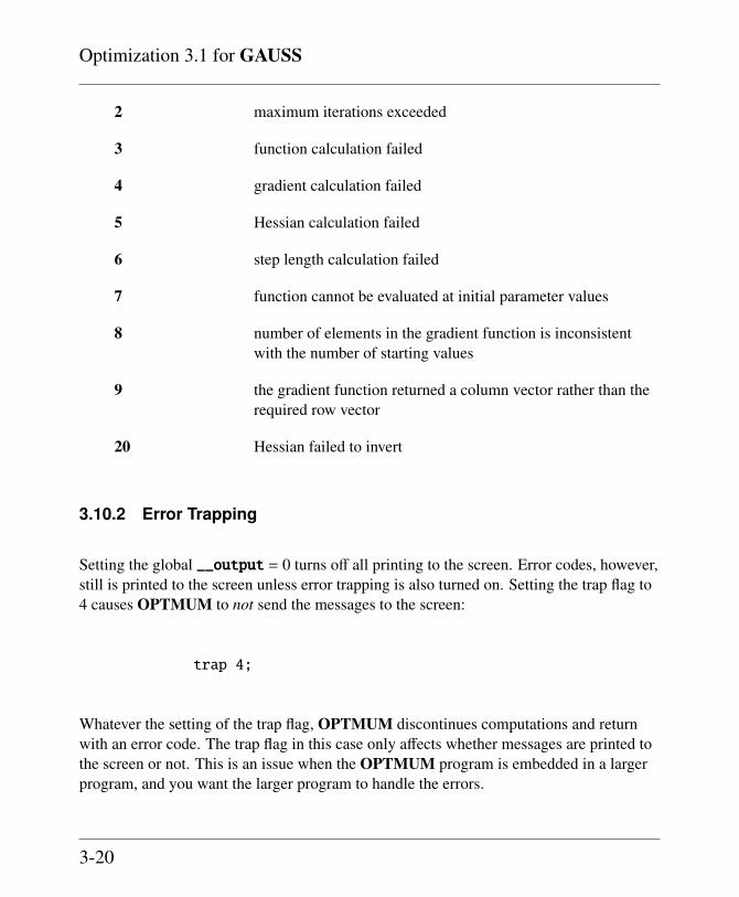
2 maximum iterations exceeded

3 function calculation failed

4 gradient calculation failed

5 Hessian calculation failed

6 step length calculation failed

7 function cannot be evaluated at initial parameter values

8 number of elements in the gradient function is inconsistentwith the number of starting values

9 the gradient function returned a column vector rather than therequired row vector

20 Hessian failed to invert

3.10.2 Error Trapping

Setting the global __output = 0 turns off all printing to the screen. Error codes, however,still is printed to the screen unless error trapping is also turned on. Setting the trap flag to4 causes OPTMUM to not send the messages to the screen:

trap 4;

Whatever the setting of the trap flag, OPTMUM discontinues computations and returnwith an error code. The trap flag in this case only affects whether messages are printed tothe screen or not. This is an issue when the OPTMUM program is embedded in a largerprogram, and you want the larger program to handle the errors.

3-20

Optim

ization

Optimization

3.11 Example

The example opt1.e is taken from D.G. Luenberger (1984) “Linear and NonlinearProgramming”, Addison-Wesley, page 219. The function to be optimized is a quadraticfunction:

f (x) = 0.5(b − x)′Q(b − x)

where a is a vector of known coefficients and Q is a symmetric matrix of knowncoefficients. For computational purposes this equation is restated:

f (x) = 0.5x′Qx − x′b

From Luenberger we set

Q =

.78 −.02 −.12 −.14−.02 .86 −.04 .06−.12 −.04 .72 −.08−.14 .06 −.08 .74

and

b′ = .76 .08 1.12 .68

First, we do the setup:

library optmum;

optset;

3-21


The procedure to compute the function is

proc qfct(x);

retp(.5*x’*Q*x-x’b);

endp;

Next a vector of starting values is defined,

x0 = { 1, 1, 1, 1 };

and finally a call to OPTMUM:

{ x,f,g,retcode } = optmum(&qfct,x0);

The estimated coefficients are returned in x, the value of the function at the minimum isreturned in f and the gradient is returned in g (you may check this to ensure that minimumhas actually been reached).

3.12 References

1. Brent, R.P., 1972. Algorithms for Minimization Without Derivatives.Englewood Cliffs, NJ: Prentice-Hall.

2. Broyden, G., 1965. “A class of methods for solving nonlinear simultaneousequations.” Mathematics of Computation 19:577-593.

3. Dennis, Jr., J.E., and Schnabel, R.B., 1983. Numerical Methods forUnconstrained Optimization and Nonlinear Equations. Englewood Cliffs,NJ: Prentice-Hall.

3-22

Optim

ization

Optimization

4. Fletcher, R. and Powell, M. 1963. “A rapidly convergent descent method forminimization.” The Computer Journal 6:163-168.

5. Gill, P. E. and Murray, W. 1972. “Quasi-Newton methods for unconstrainedoptimization.” J. Inst. Math. Appl., 9, 91-108.

6. Johnson, Lee W., and Riess, R. Dean, 1982. Numerical Analysis, 2nd Ed.Reading, MA: Addison-Wesley.

7. Luenberger, D.G., 1984. Linear and Nonlinear Programming. Reading,MA: Addison-Wesley.

3-23

Reference

Optimization Reference 4

optmum

LIBRARY optmum

PURPOSE Minimizes a user-provided function with respect to a set of parameters.

FORMAT { x,f,g,retcode } = optmum(&fct,x0);

INPUT x0 NP×1 vector, start values or the name of a proc that takes noinput arguments and returns an NP×1 vector of start values.

&fct pointer to a procedure that computes the function to beminimized. This procedure must have one input argument,an NP×1 vector of parameter values, and one output

4-1

optmum

argument, a scalar value of the function evaluated at theinput vector of parameter values.

OUTPUT x NP×1 vector, parameter estimates.

f scalar, value of function at minimum.

g NP×1 vector, gradient evaluated at x.

retcode scalar, return code. If normal convergence is achieved thenretcode = 0, otherwise a positive integer is returnedindicating the reason for the abnormal termination:

1 forced exit.2 maximum iterations exceeded.3 function calculation failed.4 gradient calculation failed.5 Hessian calculation failed.6 step length calculation failed.7 function cannot be evaluated at initial parameter values.8 number of elements in the gradient function is

inconsistent with the number of starting values.9 the gradient function returned a column vector rather

than the required row vector.20 Hessian failed to invert.

GLOBALS The globals variables used by OPTMUM can be organized in thefollowing categories according to which aspect of the optimization theyaffect:

Optimization and Steplengths _opshess, _opalgr, _opdelta,_opstmth, _opdfct, _opditer, _opmxtry, _opmdmth,_opmbkst, _opstep, _opextrp, _oprteps, _opintrp,_opusrch.

Gradient _opgdprc, _opgrdmd, _ophsprc, _opusrgd, _opusrhs.

4-2 O C R

Reference

optmum

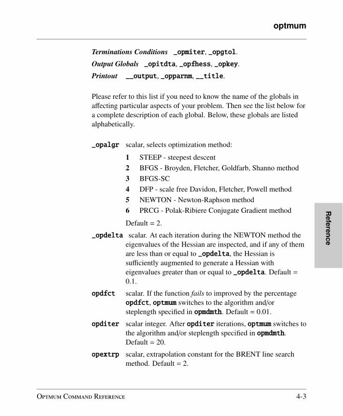
Terminations Conditions _opmiter, _opgtol.

Output Globals _opitdta, _opfhess, _opkey.

Printout __output, _opparnm, __title.

Please refer to this list if you need to know the name of the globals inaffecting particular aspects of your problem. Then see the list below fora complete description of each global. Below, these globals are listedalphabetically.

_opalgr scalar, selects optimization method:

1 STEEP - steepest descent2 BFGS - Broyden, Fletcher, Goldfarb, Shanno method3 BFGS-SC4 DFP - scale free Davidon, Fletcher, Powell method5 NEWTON - Newton-Raphson method6 PRCG - Polak-Ribiere Conjugate Gradient method

Default = 2.

_opdelta scalar. At each iteration during the NEWTON method theeigenvalues of the Hessian are inspected, and if any of themare less than or equal to _opdelta, the Hessian issufficiently augmented to generate a Hessian witheigenvalues greater than or equal to _opdelta. Default =0.1.

opdfct scalar. If the function fails to improved by the percentageopdfct, optmum switches to the algorithm and/orsteplength specified in opmdmth. Default = 0.01.

opditer scalar integer. After opditer iterations, optmum switches tothe algorithm and/or steplength specified in opmdmth.Default = 20.

opextrp scalar, extrapolation constant for the BRENT line searchmethod. Default = 2.

O C R 4-3

optmum

opfhess NP×NP matrix. Contains last Hessian calculated byoptmum. If a Hessian is never calculated, then this global isset to a scalar missing value.

opgdprc pointer to a procedure that computes the gradient of thefunction with respect to the parameters.For example, the instruction:

_opgdprc = &gradproc;

stores the pointer to a procedure with the name gradproc inopgdprc. The user-provided procedure has a single inputargument, an NP × 1 vector of parameter values, and asingle output argument, a 1 × NP row vector of gradients ofthe function with respect to the parameters evaluated at thevector of parameter values. For example, suppose theprocedure is named gradproc and the function is aquadratic function with one parameter:

y = x2 + 2x + 1

then

proc gradproc(x);

retp(2*x+2);

endp;

By default, optmum uses a numerical gradient.

opgdmd scalar, selects numerical gradient method.

0 Central difference method.1 Forward difference method.2 Forward difference method with Richardson

Extrapolation.

Default = 0.

opgtol scalar, or NP×1 vector, tolerance for gradient of estimatedcoefficients. When this criterion has been satisfied optmumexits the iterations. Default = 10−4.

4-4 O C R

Reference

optmum

ophsprc scalar, pointer to a procedure that computes the Hessian, i.e.the matrix of second order partial derivatives of the functionwith respect to the parameters.For example, the instruction:

_ophsprc = &hessproc;

stores the pointer of a procedure with the name hessproc inthe global variable ophsprc. The procedure that is providedby the user must have single input argument, the NP × 1vector of parameter values, and a single output argument,the NP × NP symmetric matrix of second order derivativesof the function evaluated at the parameter values.By default, optmum calculates the Hessian numerically.

opitdta 3×1 matrix, the first element contains the elapsed time inminutes of the iterations and the second element containsthe total number of iterations. The third element contains acharacter variable indicating the type of inverse of Hessianthat was computed:

NOCOV not computedNOTPD not positive definiteHESS computed from HessianSECANT estimated from secant update

opintrp scalar, interpolation constant for the BRENT line searchmethod. Default = 0.25.

opkey scalar, controls keyboard trapping, that is, the run-timeswitches and help table. If zero, keyboard trapping is turnedoff. This option is useful when nested copies of optmum arebeing called. Turning off the keyboard trapping of thenested copies reserves control for the outer copy of optmum.Default = 1.

opmxtry scalar, maximum number of tries to compute a satisfactorystep length. Default = 100.

O C R 4-5

optmum

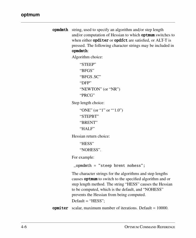
opmdmth string, used to specify an algorithm and/or step lengthand/or computation of Hessian to which optmum switches towhen either opditer or opdfct are satisfied, or ALT-T ispressed. The following character strings may be included inopmdmth:Algorithm choice:

“STEEP”“BFGS”“BFGS SC”“DFP”“NEWTON” (or “NR”)“PRCG”

Step length choice:

“ONE” (or “1” or “‘1.0”)“STEPBT”“BRENT”“HALF”

Hessian return choice:

“HESS”“NOHESS”.

For example:

_opmdmth = "steep brent nohess";

The character strings for the algorithms and step lengthscauses optmum to switch to the specified algorithm and orstep length method. The string “HESS” causes the Hessianto be computed, which is the default, and “NOHESS”prevents the Hessian from being computed.Default = “HESS”;

opmiter scalar, maximum number of iterations. Default = 10000.

4-6 O C R

Reference

optmum

opmbkst scalar, maximum number of backsteps taken to find steplength. Default = 10.

opparnm NP×1 character vector of parameter labels. By default, nolabels is used for the output.

oprteps scalar. If set to nonzero positive real number and if theselected line search method fails, then a random search istried with radius equal to the value of this global times thetruncated log to the base 10 of the gradient. Default = .01.

opshess scalar, or NP×NP matrix, the starting Hessian for BFGS,Scaled BFGS, DFP, and NEWTON. Possible scalar valuesare:

0 begin with identity matrix.1 compute starting Hessian

Default = 0. If set to a matrix, this matrix is used for thestarting Hessian. Default = 0.

opstep scalar, selects method for computing step length.

1 step length = 1.2 cubic or quadratic step length method (STEPBT)3 Brent’s step length method (BRENT)4 step halving (HALF)

Default = 2.Usually opstep = 2 is best. If the optimization bogs down,try setting opstep = 1 or 3. opstep = 3 generates slowiterations but faster convergence and opstep = 1 or 4generates fast iterations but slower convergence.When any of these line search methods fails, a randomsearch is tried with radius oprteps times the truncated logto the base 10 of the gradient. If opusrch is set to 1 optmumenters an interactive line search mode.

opstmth string, used to specify an algorithm and/or step lengthand/or computation of Hessian with which optmum begins

O C R 4-7

optmum

the iterations. The following character strings may beincluded in opstmth:Algorithm choice:

“STEEP”“BFGS”“BFGS SC”“DFP”“NEWTON” (or “NR”)“PRCG”

Step length choice:

“ONE” (or “1” or “1.0”)“STEPBT”“BRENT”“HALF”

Hessian choice:

“HESS”“NOHESS”.

The character strings for the algorithms and step lengthscauses optmum to begin with the specified algorithm and orstep length method. The string “HESS” causes the Hessianto be computed and inverted at the start of the iterations,The default setting is opstmth = “”. The default settings foropalgr, opstep, and opshess are equivalent to _opstmth= “BFGS STEPBT HESS”.

opusrch scalar. If 1, and if the selected line search method fails, thenoptmum enters an interactive line search mode. Default = 0.

opusrgd scalar, pointer to user-supplied procedure for computing anumerical gradient. This procedure has two inputarguments, a pointer to the procedure computing thefunction to be minimized and an NP × 1 vector ofcoefficients. It has one output argument, a 1 × NP row

4-8 O C R

Reference

optset

vector of derivatives of the function with respect to the NPcoefficients.

opusrhs scalar, pointer to the user-supplied procedure for computinga numerical Hessian. This procedure has two inputarguments, a pointer to the procedure computing thefunction to be minimized and an NP × 1 vector ofcoefficients. It has one output argument, an NP × NP matrixof the second derivatives of the function with respect to theNP coefficients.

_output scalar, determines printing of intermediate results.

0 nothing is written.1 serial ASCII output format suitable for disk files or

printers.2 (NOTE: Windows version only) output is suitable for

screen only. ANSI.SYS must be active.

Default = 2.

REMARKS optmum can be called recursively.

SOURCE optmum.src

optset

LIBRARY optmum

PURPOSE Resets optmum global variables to default values.

FORMAT optset;

INPUT None

O C R 4-9

optprt

OUTPUT None

REMARKS Putting this instruction at the top of all command files that invokeoptmum is generally good practice. This prevents globals from beinginappropriately defined when a command file is run several times orwhen a command file is run after another command file is executed thatcalls optmum.

optset calls gausset.

SOURCE optmum.src

optprt

LIBRARY optmum

PURPOSE Formats and prints the output from a call to optmum.

FORMAT { x,f,g,retcode } = OPTPRT(x,f,g,retcode);

INPUT x NP×1 vector, parameter estimates.

f scalar, value of function at minimum.

g NP×1 vector, gradient evaluated at x.

retcode scalar, return code.

OUTPUT Same as Input.

GLOBALS _title string, title of run. By default, no title is printed.

REMARKS The call to optmum can be nested in the call to optprt:

4-10 O C R

Reference

gradfd

{ x,f,g,retcode } = optprt(optmum(&fct,x0));

This output is suitable for a printer or disk file.

SOURCE optmum.src

gradfd

LIBRARY optmum

PURPOSE Computes the gradient vector or matrix (Jacobian) of a vector-valuedfunction that has been defined in a procedure. Single-sided (forwarddifference) gradients are computed.

FORMAT d = gradfd(&f,x0);

INPUT &f procedure pointer to a vector-valued function:

f : RK → RN

It is acceptable for f (x) to have been defined in terms ofglobal arguments in addition to x, and thus f can return anN×1 vector:

proc f(x);

retp( exp(x*b) );

endp;

x0 NP×1 vector, point at which to compute gradient.

OUTPUT g N×NP matrix, gradients of f with respect to the variable x atx0.

O C R 4-11

gradfd

GLOBALS grdh scalar, determines increment size for numerical gradient. Bydefault, the increment size is automatically computed.

REMARKS gradfd returns a ROW for every row that is returned by f . Forinstance, if f returns a 1×1 result, then gradfd returns a 1×NP rowvector. This allows the same function to be used where N is the numberof rows in the result returned by f . Thus, for instance, gradfd can beused to compute the Jacobian matrix of a set of equations.

To use gradfd with optmum, put


at the top of the command file, and

_opusrgd = &gradfd;

somewhere in the command file after the call to optset and before thecall to optmum. For example,

library optmum;

#include optmum.ext


optset;

start = { -1, 1 };

proc fct(x);

local y1,y2;

y1 = x[2] - x[1]*x[1];

y2 = 1 - x[1];

4-12 O C R

Reference

gradcd

retp (1e2*y1*y1 + y2*y2);

endp;

_opusrgd = &gradfd;

{ x,fmin,g,retcode } = optprt(optmum(&fct,start));

optmum uses the central difference method when opgdmd = 1, thususing gradfd as it is written is redundant. Its use would beadvantageous, however, if you were to modify gradfd for a specialpurpose.

SOURCE gradient.src

gradcd

LIBRARY optmum

PURPOSE Computes the gradient vector or matrix (Jacobian) of a vector-valuedfunction that has been defined in a procedure. Central differencegradients are computed.

FORMAT d = gradcd(&f,x0);


f : RNP → RN


O C R 4-13

gradcd

proc f(x);

retp( exp(x*b) );

endp;

x0 NP×1 vector, points at which to compute gradient.


GLOBALS grdh scalar, determines increment size for numerical gradient. Bydefault, the increment size is automatically computed.

REMARKS gradcd returns a ROW for every row that is returned by f . Forinstance, if f returns a 1×1 result, then gradcd returns a 1×NP rowvector. This allows the same function to be used where N is the numberof rows in the result returned by f . Thus, for instance, gradcd can beused to compute the Jacobian matrix of a set of equations.

To use gradcd with optmum, put



_opusrgd = &gradcd;


library optmum;

#include optmum.ext

4-14 O C R

Reference

gradre


optset;

start = { -1, 1 };

proc fct(x);

local y1,y2;

y1 = x[2] - x[1]*x[1];

y2 = 1 - x[1];

retp (1e2*y1*y1 + y2*y2);

endp;

_opusrgd = &gradcd;


optmum uses the central difference method when opgdmd = 1, thususing gradcd as it is written is redundant. Its use would beadvantageous, however, if you were to modify gradcd for a specialpurpose.

SOURCE gradient.src

gradre

LIBRARY optmum

PURPOSE Computes the gradient vector or matrix (Jacobian) of a vector-valuedfunction that has been defined in a procedure. Single-sided (forwarddifference) gradients are computed, using Richardson Extrapolation.

O C R 4-15

gradre

FORMAT d = gradre(&f,x0);


f : RNP → RN


proc f(x);

retp( exp(x*b) );

endp;

x0 NP×1 vector, points at which to compute gradient.


GLOBALS _grnum integer, determines the number of iterations algorithmproduces. Beyond a certain point, increasing _grnum doesnot improve accuracy of result; on the contrary, round errorswamps accuracy and results become significantly worse.

_grsca scalar, between 0 and 1. By reducing _grsca, algorithmmay arrive at an acceptable result sooner, but this may notbe as accurate as a result achieved with larger _grsca andwhich might take longer to compute. Generally, an _grscamuch smaller than 0.05 does not improve resultssignificantly.

_grstp scalar, should be less than 1. The best results seemed to beobtained most efficiently when _grstp is between 0.4 and0.8. Changing _grstp and _grsca may have positiveeffects on results of algorithm.

REMARKS The settings for the global variables, for a reasonably well-definedproblem, produces convergence with moderate speed. If the problem is

4-16 O C R

Reference

gradre

difficult and doesn’t converge then try setting _grnum to 20, _grsca to0.4, and _grstp to 0.5. This slows down the computation of thederivatives by a factor of 3 but increases the accuracy to near that ofanalytical derivatives.

gradre returns a ROW for every row that is returned by f . Forinstance, if f returns a 1×1 result, then gradre returns a 1×NP rowvector. This allows the same function to be used where N is the numberof rows in the result returned by f . Thus, for instance, gradre can beused to compute the Jacobian matrix of a set of equations.

The algorithm, Richardson Extrapolation (see Numerical Analysis, byLee W. Johnson and R. Dean Riess, page 319) is an iterative processwhich updates a derivative based on values calculated in a previousiteration. This is slower than gradp, but can, in general, return valuesthat are accurate to about 8 digits of precision. The algorithm runsthrough n iterations. grnum is a global whose default is 25.


proc myfunc(x);

retp( x.*2 .* exp( x.*x./3));

endp;

x0 = { 2.5, 3.0, 3.5 };

y = gradre(&myfunc,x0);

print y;

82.98901642 0.00000000 0.00000000

0.00000000 281.19752454 0.00000000

0.00000000 0.00000000 1087.95412226

To use gradre with optmum, put

O C R 4-17

gradre



_opusrgd = &gradre;


library optmum;

#include optmum.ext


optset;

start = { -1, 1 };

proc fct(x);

local y1,y2;

y1 = x[2] - x[1]*x[1];

y2 = 1 - x[1];

retp (1e2*y1*y1 + y2*y2);

endp;

_opusrgd = &gradre;


SOURCE gradient.src

4-18 O C R

Index

Index

Index

algorithm, 3-2, 3-18Alt-1, 3-18Alt-2, 3-19Alt-3, 3-19Alt-4, 3-19Alt-5, 3-19Alt-6, 3-19ALT-A, 3-18ALT-H, 3-18

B

backstep, 3-18backsteps, 4-7BFGS, 3-5, 3-19, 4-3, 4-7BFGS, scaled, 4-3BFGS-SC, 3-19BRENT, 3-19

C

central difference, 4-4conjugate gradient, 3-6convergence, 4-7cubic step, 4-7

D

derivatives, 3-14DFP, 3-5, 3-19, 4-3, 4-7

F

forward difference, 4-4

G

global variables, 3-18gradcd, 4-13gradfd, 3-14, 4-11gradient, 4-2, 4-4, 4-10, 4-11, 4-13, 4-15gradre, 4-15_grdh, 4-12, 4-14_grnum, 3-16_grsca, 3-16_grstp, 3-16

H

HALF, 3-19Hessian, 3-18, 4-5, 4-7

Index-1

Index

I

increment size, 4-12, 4-14Installation, 1-1

L

line search, 3-7

M

mid-method, 3-18

N

NEWTON, 3-5Newton, 3-5NEWTON, 3-19, 4-3, 4-7Newton-Raphson, 3-19NR, 3-19

O

_opalgr, 4-3_opdelta, 4-3_opdfct, 3-11, 3-13, 3-17, 3-18_opditer, 3-11, 3-13, 3-17, 3-18opextrp, 4-3opfhess, 4-4_opgdmd, 3-18opgdmd, 4-4opgdprc, 4-4_opgtol, 3-18opgtol, 4-4_ophsprc, 3-17ophsprc, 4-5opintrp, 4-5

opitdta, 4-5_opkey, 3-9opkey, 4-5opmbkst, 4-7_opmdmth, 3-11, 3-12, 3-17opmiter, 4-6opmxtry, 4-5opparnm, 4-7oprteps, 4-7_opshess, 3-17opshess, 4-7opstep, 4-7_opstmth, 3-11, 3-12optmum, 4-1optprt, 4-10optset, 4-9opusrch, 4-8opusrgd, 4-8opusrhs, 4-9__output, 3-18_output, 4-9

P

PRCG, 3-6, 3-19, 4-3

Q

quadratic step, 4-7

R

random search, 3-8run-time switches, 3-18

Index-2

Index

Index

S

Scaled BFGS, 4-7SD, 4-3SHIFT-1, 3-19SHIFT-2, 3-19SHIFT-3, 3-19SHIFT-4, 3-19start values, 4-1starting point, 3-11STEEP, 3-4, 3-18Steepest Descent, 3-4step length, 3-7, 3-18, 4-7STEPBT, 3-19

T

_title, 4-10

U

UNIX, 1-3UNIX/Linux/Mac, 1-1

W

Windows, 1-2, 1-3

Index Index-3

optimization 3 - gauss · 3.1.4 polak-ribiere-type conjugate gradient ... if you are unfamiliar...

Documents