optimization and control of reservoir models using system

OPTIMIZATION AND CONTROL OF RESERVOIR MODELS USING SYSTEM

IDENTIFICATION AND MACHINE LEARNING TOOLS

Luis Kin Miyatake

Dissertacao de Mestrado apresentada ao

Programa de Pos-graduacao em Engenharia

Eletrica, COPPE, da Universidade Federal do

Rio de Janeiro, como parte dos requisitos

necessarios a obtencao do tıtulo de Mestre em

Engenharia Eletrica.

Orientador: Amit Bhaya

Rio de Janeiro

Julho de 2019



Luis Kin Miyatake

DISSERTACAO SUBMETIDA AO CORPO DOCENTE DO INSTITUTO

ALBERTO LUIZ COIMBRA DE POS-GRADUACAO E PESQUISA DE

ENGENHARIA (COPPE) DA UNIVERSIDADE FEDERAL DO RIO DE

JANEIRO COMO PARTE DOS REQUISITOS NECESSARIOS PARA A

OBTENCAO DO GRAU DE MESTRE EM CIENCIAS EM ENGENHARIA

ELETRICA.

Examinada por:

Prof. Amit Bhaya, Ph. D.

Prof. Luis Antonio Aguirre, Ph. D.

Prof. Ramon Romankevicius Costa, D. Sc.

Prof. Alexandre Anoze Emerick, Ph. D.

RIO DE JANEIRO, RJ – BRASIL

JULHO DE 2019

Miyatake, Luis Kin

Optimization and Control of Reservoir Models using

System Identification and Machine Learning Tools/Luis

Kin Miyatake. – Rio de Janeiro: UFRJ/COPPE, 2019.

XVII, 75 p.: il.; 29, 7cm.


Dissertacao (mestrado) – UFRJ/COPPE/Programa de

Engenharia Eletrica, 2019.

Referencias Bibliograficas: p. 73 – 75.

1. System Identification. 2. Optimization. 3.

Machine Learning. I. Bhaya, Amit. II. Universidade

Federal do Rio de Janeiro, COPPE, Programa de

Engenharia Eletrica. III. Tıtulo.

iii

Acknowledgement

Gostaria de agradecer, inicialmente, ao professor Amit Bhaya, meu orientador do

programa de engenharia eletrica da Coppe/UFRJ. Obrigado pelas recomendacoes

de materias, pelas sugestoes elegantes e por toda atencao concedida durante estes

dois anos.

Tambem sou grato aos profissionais do Petrobras/Cenpes pelas sugestoes de

trabalho. Em especial, aos engenheiros Mario Campos, Emerick, Manuel Fragoso e

Alex Teixeira, bem como ao gerente Ziglio pelo incentivo ao longo desta jornada.

A minha mae, que sempre depositou grande confianca no meu esforco e forca de

vontade. A Isis, pela compreensao e bom humor. A Deus e a todos aqueles que me

ajudaram ate aqui.

iv

Resumo da Dissertacao apresentada a COPPE/UFRJ como parte dos requisitos

necessarios para a obtencao do grau de Mestre em Ciencias (M.Sc.)

OTIMIZACAO E CONTROLE DE MODELOS DE RESERVATORIOS USANDO

TECNICAS DE IDENTIFICACAO DE SISTEMAS E APRENDIZADO DE

MAQUINA

Luis Kin Miyatake

Julho/2019


Programa: Engenharia Eletrica

Este trabalho desenvolve uma metodologia, usando conceitos de identificacao

de sistemas dinamicos, para criar modelos substitutos (conhecidos como proxy) de

reservatorios de oleo e gas considerando-se variaveis controladas, tais como vazoes de

lıquido e injetadas. Os principais objetivos sao previsao e otimizacao da producao.

Os metodos classicos de ajuste de historico consideram o ajuste de parametros de

um modelo de simulacao de fluxo em meios porosos. Em contraste, essa dissertacao

propoe avaliar o uso de modelos do tipo proxy, com dois enfoques diferentes: o

primeiro e baseado puramente em entrada e saıda, ao passo que o segundo leva

em conta o espaco de estados de uma simulacao numerica, ambos usando dados

provenientes da simulacao numerica de um modelo de reservatorios.

Seguindo o princıpio da parcimonia, representacoes mais simples, tais como ARX

e ARMAX, sao avaliadas inicialmente para os modelos entrada-saıda. Para modelos

baseados em estados, realiza-se reducao de dimensionalidade, atraves do metodo con-

hecido como POD (proper orthogonal decomposition). As matrizes de um modelo

proxy linear sao identificadas nos estados de dimensao reduzida, o que nos permite

formular um problema de otimizacao, cuja funcao objetivo e maximizar uma funcao

economica VPL (valor presente lıquido), como uma sequencia de problemas do tipo

programacao linear, dentro de um arcabouco de um metodo de otimizacao baseado

em regiao de confianca.

Algumas contribuicoes, mostradas ao longo dessa dissertacao, incluem um

metodo expedito para avaliacao de incertezas, analise da adaptacao dos coeficientes

do filtro RLS (mınimos quadrados recursivos) em termos fısicos para o problema,

bem como insights sobre selecao de modelos e incorporacao de conhecimento a priori.

v

Abstract of Dissertation presented to COPPE/UFRJ as a partial fulfillment of the

requirements for the degree of Master of Science (M.Sc.)



Luis Kin Miyatake

July/2019

Advisor: Amit Bhaya

Department: Electrical Engineering

This dissertation develops a methodology to identify a dynamical system mod-

eling an oil and gas reservoir, subject to production controls such as water injection

rate and liquid production rate. The overall objectives are to improve production

forecasts and decision making processes regarding the development of the field, such

as future control strategies and “what-if” analyses considering different scenarios.

The classical history matching approach uses numerical simulation and tuning

of geological parameters. In contrast, this dissertation proposes the use of a system

identification approach to build two proxy models, one based on the input-output

approach and the other on a state-space approach, both utilizing data that comes

from a simulator used in industry. In accordance with the parsimony principle,

simpler polynomial model structures such as ARX and ARMAX are used for the

input-output model.

The linear state space model uses states coming from model simulation as its data

for identification, and is subjected to model reduction using the proper orthogonal

decomposition (POD) method. This linear state space reduced order proxy model

is then used to formulate an optimal control problem, solved by transcription into a

sequence of linear programs using a trust region algorithm, maximizing Net Present

Value, which is an objective function representing the overall economic performance

of the production process.

Additional significant contributions, developed in the course of this dissertation,

include a fast method for uncertainty estimation, analysis of RLS coefficient adap-

tation to get physical insights into the correlation between producer and injector

wells, as well as insights into model selection and incorporation of prior knowledge.

vi

Contents

List of Figures ix

List of Tables xv

1 Introduction and Literature Review 1

2 Discrete-time linear system models for identification: practical ex-

amples 7

2.1 Introduction . . . . . . . . . . . . . . . . . . . . . . . . . . . . . . . . 7

2.2 Preliminaries on input-output discrete time models for identification . 8

2.2.1 ARX models . . . . . . . . . . . . . . . . . . . . . . . . . . . . 8

2.2.2 ARMAX models . . . . . . . . . . . . . . . . . . . . . . . . . 8

2.3 Training algorithms for ARX and ARMAX models . . . . . . . . . . 9

2.3.1 Training an ARX model . . . . . . . . . . . . . . . . . . . . . 9

2.3.2 ARMAX training procedure . . . . . . . . . . . . . . . . . . . 10

2.4 Model Structure Selection . . . . . . . . . . . . . . . . . . . . . . . . 10

2.5 Estimation of Parameter Uncertainty . . . . . . . . . . . . . . . . . . 12

2.5.1 Covariance Matrix Estimation . . . . . . . . . . . . . . . . . . 13

2.5.2 Sampling on the boundary of the uncertainty ellipsoid . . . . . 14

2.6 Online Learning . . . . . . . . . . . . . . . . . . . . . . . . . . . . . . 15

2.6.1 Recursive Least Squares . . . . . . . . . . . . . . . . . . . . . 15

2.6.2 Practical Remarks about the Prior Knowledge in the RLS filters 18

2.7 Simulator-based identification and validation of reservoir models . . . 18

2.7.1 Choice of Features and Experimental Design . . . . . . . . . . 19

2.7.2 Results of ARX and ARMAX modeling . . . . . . . . . . . . . 20

3 Proxy States Based Model 37

3.1 Method of snapshots . . . . . . . . . . . . . . . . . . . . . . . . . . . 37

3.2 Relation between Regularization and PCA . . . . . . . . . . . . . . . 39

3.3 State Matrix Estimation . . . . . . . . . . . . . . . . . . . . . . . . . 40

3.3.1 Output Identification . . . . . . . . . . . . . . . . . . . . . . . 41

3.4 Proxy based Optimization . . . . . . . . . . . . . . . . . . . . . . . . 42

vii

3.5 Results . . . . . . . . . . . . . . . . . . . . . . . . . . . . . . . . . . . 44

3.5.1 Assessment of Proxy Model . . . . . . . . . . . . . . . . . . . 44

3.5.2 Optimization Results . . . . . . . . . . . . . . . . . . . . . . . 61

4 Conclusions and Future Work 70

Bibliography 73

viii

List of Figures

1.1 Case 1: Input-Output schematics, where WIR (Water injection Rate)

is a PRBS excitation and LPR (liquid production rate) is constant.

As a result, BHP (bottom hole pressure) is a variable output, as is

WC (water cut). . . . . . . . . . . . . . . . . . . . . . . . . . . . . . 2

1.2 Case 2: Input-Output schematics, where WIR (Water injection Rate)

is a PRBS excitation and BHP (bottom hole pressure) is constant.

As a result, LPR (liquid production rate) is a variable output, as is

WC (water cut). . . . . . . . . . . . . . . . . . . . . . . . . . . . . . 2

1.3 Case 3: Input-Output schematics, where both WIR (Water injection

Rate) and LPR (liquid production rate) are PRBS Excitation. As a

result, BHP (bottom hole pressure) is a variable output, as is WC

(water cut). . . . . . . . . . . . . . . . . . . . . . . . . . . . . . . . . 2

1.4 Case 4: Input-Output schematics, where both WIR (Water injection

Rate) and BHP (bottom hole pressure) are PRBS Excitation. As a

result, LPR (liquid production rate) is a variable output, as is WC

(water cut). . . . . . . . . . . . . . . . . . . . . . . . . . . . . . . . . 2

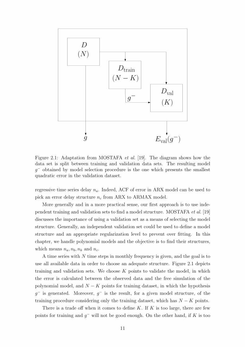
2.1 Adaptation from MOSTAFA et al. [19]. The diagram shows how

the data set is split between training and validation data sets. The

resulting model g− obtained by model selection procedure is the one

which presents the smallest quadratic error in the validation dataset. 11

2.2 Water Injection Rates PRBS Excitation for System Identification.

The Liquid Producer Rates are kept constant. . . . . . . . . . . . . . 19

2.3 Water saturation map is represented during 14 years. It is worthwhile

pointing out the time variant characteristics of the production system,

which varies especially when water breakthrough occurs. . . . . . . . 20

2.4 Reference log-permeability field, making evident the permeability

path connectivity between INJ-01 and PRO-02/PRO-03 and INJ-02

and PRO-04/PRO-05. . . . . . . . . . . . . . . . . . . . . . . . . . . 21

2.5 Model Structure choice based on the Validation Set for the producer

well PRO-01. . . . . . . . . . . . . . . . . . . . . . . . . . . . . . . . 21

ix

2.6 Chosen the model structure, training and validation data set are used

for training. Residual analysis indicates that the error is a white noise

for the producer well PRO-01. . . . . . . . . . . . . . . . . . . . . . . 22

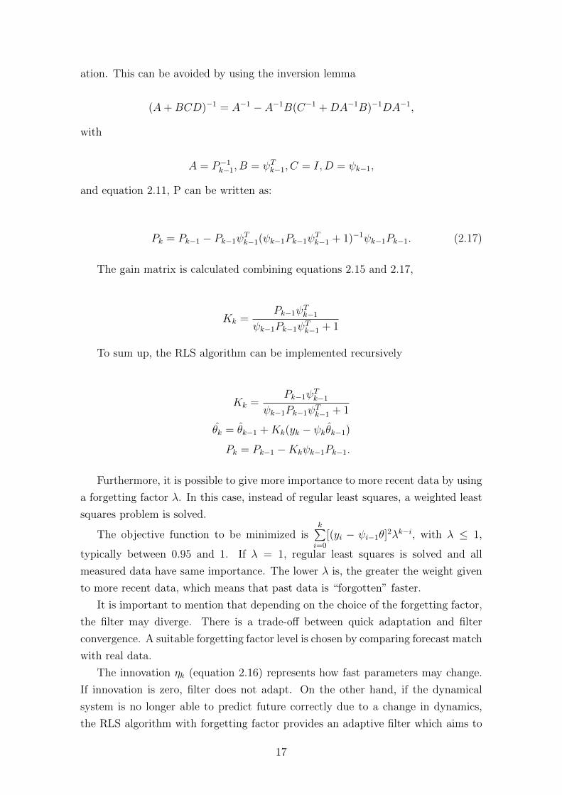
2.7 Test set assessment comparing the forecast on the average case (in

black) and Test Data Set. In green, 50 different parameter vectors

with the same model structure were sampled on the Ellipsoid of Un-

certainty considering 3 standard deviation for the producer PRO-01. . 23

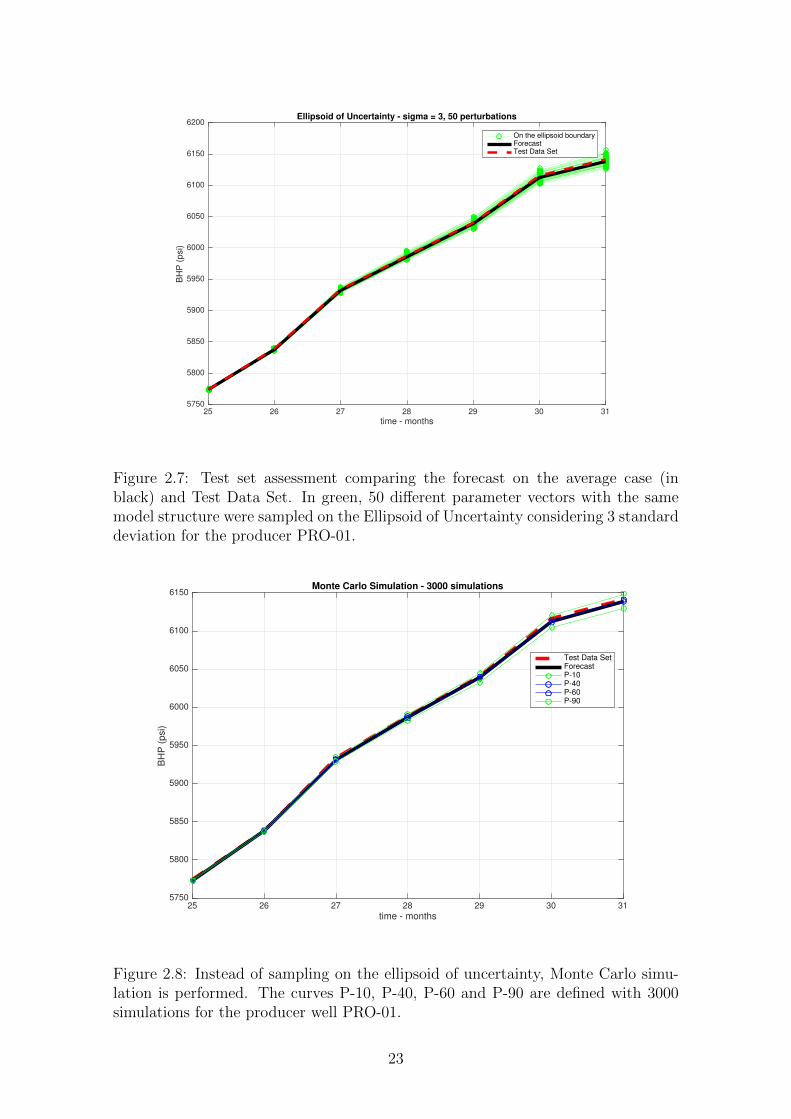
2.8 Instead of sampling on the ellipsoid of uncertainty, Monte Carlo simu-

lation is performed. The curves P-10, P-40, P-60 and P-90 are defined

with 3000 simulations for the producer well PRO-01. . . . . . . . . . 23

2.9 Step Response: BHP - PRO-01. Both INJ-01 and INJ-02 contribute

for BHP increase for the producer well PRO-01 in the step response. . 24

2.10 Model Structure choice based on the Validation Set for the producer

well PRO-02. . . . . . . . . . . . . . . . . . . . . . . . . . . . . . . . 25

2.11 Chosen the model structure, training and validation data set are used

for training. Residual analysis indicates that the error is not very

different from a white noise for the producer well PRO-02. . . . . . . 26


black) and Test Data Set. In green, 50 different parameter vectors

with the same model structure were sampled on the Ellipsoid of Un-

certainty considering 3 standard deviation for the producer well PRO-

02. It is worthwhile mentioning the scale, which ranges from 0.90 to

0.94, indicating a good agreement between the uncertainty analysis

forecast and the test data set. . . . . . . . . . . . . . . . . . . . . . . 26

2.13 Instead of sampling on the ellipsoid of uncertainty, Monte Carlo simu-

lation is performed. The curves P-10, P-40, P-60 and P-90 are defined

with 3000 simulations for the producer PRO-02. . . . . . . . . . . . . 27

2.14 Step Response for the producer wel PRO-02. INJ-01 has a meaningful

contribution for water cut increase in PRO-02, whereas INJ-02 seems

to have very little influence. . . . . . . . . . . . . . . . . . . . . . . . 27

2.15 The graph shows 3 different choices for forgetting factors in the RLS

filter. 12 months ahead prediction of water cut for the producer PRO-

03 (in blue) is compared with the original time series, which comes

from the model simulation. . . . . . . . . . . . . . . . . . . . . . . . . 28

2.16 RLS - Exogenous Parameters Adaptation for the producer PRO-03.

Interestingly, we see a pattern change after the water breakthrough,

which means the filter adapts quickly and is able to capture the real

connectivity among the wells. . . . . . . . . . . . . . . . . . . . . . . 29

x

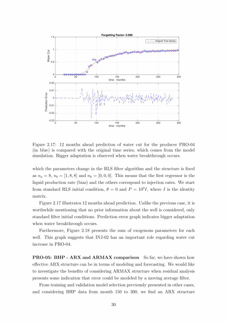
2.17 12 months ahead prediction of water cut for the producer PRO-04

(in blue) is compared with the original time series, which comes from

the model simulation. Bigger adaptation is observed when water

breakthrough occurs. . . . . . . . . . . . . . . . . . . . . . . . . . . . 30

2.18 The evolution of the sum of exogenous parameters for each well for the

producer PRO-04. Because the standard initial condition was chosen

(θ = 0, P = 103I) the filter starts to learn from data when water

breakthrough occurs. Until then, the output water cut is zero and

there is no information to be learnt from. The parameters successfully

indicate connectivity between INJ-02 and PRO-04. . . . . . . . . . . 31


black) and Test Data Set. In green, 50 different models were sampled

on the Ellipsoid of Uncertainty considering 3 standard deviation for

the producer PRO-05. . . . . . . . . . . . . . . . . . . . . . . . . . . 32

2.20 Residual analysis indicates 1-period lag out of ACF bounds, which

suggests that error could be modeled with a moving average (MA)

component. This is why we attempt to model it evolving from ARX

structure to ARMAX. . . . . . . . . . . . . . . . . . . . . . . . . . . 33


black) and Test Data Set. In green, 50 different models were sampled

on the Ellipsoid of Uncertainty considering 3 standard deviation for

the producer PRO-05 using the ARMAX model. . . . . . . . . . . . . 34

2.22 In fact, ARMAX model presents suitable results in residual analysis,

which means choosing nc = 1 successfully models the error. . . . . . 34

2.23 Comparison between ARX and ARMAX in the test data set. Despite

its advantage of modeling the error, ARMAX presents results very

similar to ARX in free simulation in the test data set. . . . . . . . . . 35

2.24 Observed Data and Prior Knowledge Data Set. Prior Knowledge

may come from different sources, such as a numerical model reservoir

simulation or another well with a large history data set with similar

characteristics. . . . . . . . . . . . . . . . . . . . . . . . . . . . . . . 35

2.25 12 months ahead prediction of the Field Oil Rate considering Stan-

dard RLS filter Initial Condition (θ = 0, P = 103I). . . . . . . . . . . 36

2.26 12 months ahead prediction of the Field Oil Rate considering Initial

Condition from data assimilation of a prior knowledge data set, as

depicted in 2.24. . . . . . . . . . . . . . . . . . . . . . . . . . . . . . . 36

xi

3.1 Pseudo Random Binary Sequence (PRBS) Excitation considering

both producer and injector wells. This graph represents LPR (liquid

production rate) for all producer wells (from PRO-01 to PRO-06) and

WIR (water injection rate) for all injector wells (INJ-01 and INJ-02). 46

3.2 Singular Value Decomposition - from the greatest singular value to

the smallest. The dimensionality was reduced from 450 to 19 for water

saturation and to 29 for block pressure, which simplifies the identi-

fication problem and prevents from overfitting. The energy retained

ε (which defines the dimension of the POD-basis) is chosen based on

the maps reconstruction assessment for both water saturation and

block pressure maps, as shown in Figures 3.3 - 3.9. . . . . . . . . . . 48

3.3 The first row shows water saturation evolution according to the proxy

model, the second according to the simulated model and the last row

shows the difference between the two, for the case in which the box

constraint allows zero (∆0u) deviation from reference trajectory. . . . . 49




constraint allows deviation±100 barrels per day (∆100u ) from reference

trajectory. . . . . . . . . . . . . . . . . . . . . . . . . . . . . . . . . . 50





trajectory. . . . . . . . . . . . . . . . . . . . . . . . . . . . . . . . . . 51





trajectory. . . . . . . . . . . . . . . . . . . . . . . . . . . . . . . . . . 52

3.7 The first row shows block pressure (in psi) evolution according to the

proxy model, the second according to the simulated model and the

last row shows the difference between the two, for the case in which

the box constraint allows zero deviation (∆0u) from reference trajectory. 54




the box constraint allows a deviation of ±25 barrels per day (∆25u )

from reference trajectory. . . . . . . . . . . . . . . . . . . . . . . . . . 55

xii




the box constraint allows a deviation of ±50 barrels per day (∆50u )

from reference trajectory. . . . . . . . . . . . . . . . . . . . . . . . . . 56

3.10 For all producer wells, the output variable is oil production rate. The

figure compares the output of the proxy model with the simulated

one. In green, the control (liquid production rate) resulted from the

LP problem is shown in the case in which the box constraint allows

zero deviation (∆0u) from reference trajectory. . . . . . . . . . . . . . 57





a deviation of ±100 barrels per day (∆100u ) from reference trajectory. . 58





a deviation of ±200 barrels per day (∆200u ) from reference trajectory. . 59





a deviation of ±300 barrels per day (∆300u ) from reference trajectory.

As the allowed deviation is larger, the proxy model tends to present

larger deviations from the simulation model. . . . . . . . . . . . . . . 60

3.14 The first graph shows the rapid initial increase of the NPV due to

the optimization algorithm achieving 9.1% overall gain. The second

graph compares optimal cumulative oil production (blue curve) and

initial solution (black curve). The third graph shows Total Liquid

Production Rate attaining its upper bound (Liquid Capacity Con-

straint) and the fourth graph shows Total Injection Rate. . . . . . . . 62

3.15 Figure shows the evolution of the trajectory controls (liquid produc-

tion rate for producers PRO-01, PRO-02, PRO-03 and PRO-04) for

all iterations in the trust region algorithm, from the initial condition

(iter 1) to the final solution (iter 15). . . . . . . . . . . . . . . . . . . 64

xiii

3.16 Figure shows the evolution of the trajectory control (liquid produc-

tion rate for producers PRO-05 and PRO-06 and water injection rate

for injector INJ-01 and INJ-02) for all iterations in the trust region

algorithm, from the initial condition (iter 1) to the final solution (iter

15). . . . . . . . . . . . . . . . . . . . . . . . . . . . . . . . . . . . . . 65

3.17 For a liquid capacity constraint of 11350 BPD, the graph indicates the

water cut for all producer wells. For most wells, the solution derived

from the trust region algorithm results in water breakthrough being

delayed, which explains the gains in field cumulative oil production

and the net present value (NPV). . . . . . . . . . . . . . . . . . . . . 66

3.18 In the first graph, the sensitivity analysis shows the NPV Gain evo-

lution when the Total Liquid Capacity constraint is increased. The

second graph shows the total liquid production for different total liq-

uid capacities. Interestingly, when the capacity is 14200 BPD, this

constraint is not active during the entire period. . . . . . . . . . . . . 68

3.19 For all wells, both producers and injectors, the graph shows the trajec-

tory controls (liquid production rate for producers and water injection

rates for injectors) for different total liquid capacity constraints. No-

tice that the trajectory controls are not intuitively obvious, especially

for different scenarios. . . . . . . . . . . . . . . . . . . . . . . . . . . 69

xiv

List of Tables

2.1 Range of perturbation . . . . . . . . . . . . . . . . . . . . . . . . . . 19

3.1 Liquid Rate Bounds (BPD) . . . . . . . . . . . . . . . . . . . . . . . 61

3.2 Sensitivity Analysis . . . . . . . . . . . . . . . . . . . . . . . . . . . . 67

xv

List of Symbols

u Current trajectory control

∆u Box constraint in which the proxy model is valid around u

ε Percentage of energy retained for dimensionality reduction

λ Forgetting factor in the RLS algorithm

ρ Proxy Quality Control Index

A(q) Auto regressive polynomial of ARX model

B(q) Exogenous polynomial of ARX model

C(q) Error polynomial of ARMAX model

E Uncertainty ellipsoid corresponding to 1 standard deviation

Eval Error calculated in the validation data set

LP Linear Programming Problem

Qmax Platform liquid capacity constraint

sr Slew Rate, a constraint which imposes smoothness in the trajectory control

Ur Reduced matrix from POD dimensionality reduction procedure

X Snapshot Matrix

ACF Autocorrelation Function

ARMAX Auto Regressive Moving Average Exogenous Model

ARX Auto Regressive Exogenous Model

BHP Bottom hole pressure

BPD Barrels per day

xvi

ELS Extended Least Squares

NPV Net Present Value

POD Proper Orthogonal Decomposition

PRBS Pseudorandom Binary Sequence

WC Water Cut

xvii

Chapter 1

Introduction and Literature

Review

Reservoir modeling is concerned with the construction of a computer model of an

oil and gas reservoir, with the aim of improving estimation of reserves, production

forecasting and decision making processes regarding the development of the field,

such as well placement, future control strategies and “what if” analyses considering

different scenarios.

A reservoir model consists of grid blocks, which represent the physical space

where the reservoir is located, and each grid block has parameters (porosity, per-

meability and so forth) and states (pressure, water saturation, oil saturation etc).

The reservoir model solves a finite difference numerical scheme derived from a par-

tial differential equation, which models the spatiotemporal evolution in the porous

media, considering its different phases and compositions.

Typically, an oil and gas field has producer and injector wells. The producers

produce liquid (oil and water) and gas, and the injectors inject water, gas or both

in alternate cycles. The importance of the injectors is related to the maintenance

of the reservoir pressure and oil displacement. If it were not for them, the average

pressure in the reservoir would drop, and the oil recovery would worsen.

However, as the injectors start injecting water or gas, the water (or gas) front

reaches the producer well. This moment is called water (or gas) breakthrough. Of

course, this causes an increase in the water cut ratio (ratio between produced water

rate and produced liquid rate), as well as gas oil ratio increase.

In terms of what can actually be measured, the output variables of a reservoir

are generally oil, water and gas well rates, as well as the bottom hole pressure

(BHP) and compositional contents. These variables, measured in hourly, daily or

even monthly frequencies are modeled as outputs of suitable state variables, which

evolve according to a dynamical system.

For the sake of identification, it is suitable to excite the reservoir system with

1

Reservoir ModelWIR PRBS Excitation

LPR constant

WCBHP variable

Figure 1.1: Case 1: Input-Output schematics, where WIR (Water injection Rate) isa PRBS excitation and LPR (liquid production rate) is constant. As a result, BHP(bottom hole pressure) is a variable output, as is WC (water cut).

Reservoir ModelWIR PRBS Excitation

BHP constant

WCLPR variable

Figure 1.2: Case 2: Input-Output schematics, where WIR (Water injection Rate) isa PRBS excitation and BHP (bottom hole pressure) is constant. As a result, LPR(liquid production rate) is a variable output, as is WC (water cut).

Reservoir ModelWIR PRBS ExcitationLPR PRBS Excitation

WCBHP variable

Figure 1.3: Case 3: Input-Output schematics, where both WIR (Water injectionRate) and LPR (liquid production rate) are PRBS Excitation. As a result, BHP(bottom hole pressure) is a variable output, as is WC (water cut).

Reservoir ModelWIR PRBS ExcitationBHP PRBS Excitation

WCLPR variable

Figure 1.4: Case 4: Input-Output schematics, where both WIR (Water injectionRate) and BHP (bottom hole pressure) are PRBS Excitation. As a result, LPR(liquid production rate) is a variable output, as is WC (water cut).

2

a PRBS (pseudo random binary sequence) signal. The figures 1.1, 1.2, 1.3 and 1.4

show configurations of possible excitation scenarios, provided that model simulation

considers as input variables either flow rate or bottom hole pressure for injector and

producer wells.

System identification (SI) is a methodology to build mathematical models of

a dynamical system based on measurements of input and output signals. System

identification models tend to be simpler than their counterparts based on detailed

models using the physics of the underlying phenomena followed by numerical simu-

lation. When a long history of input-output measurements is available, SI models,

despite their relative simplicity, can be accurate enough for the purposes of control

and optimization (more details in ZHOU et al. [1]).

This work uses system identification concepts for reservoir modeling. Two dif-

ferent approaches are presented: the first one, discussed in chapter 2, estimates a

transfer function between inputs and outputs, whereas the second one, discussed in

chapter 3, tackles the development of a proxy model based on numerical simulation

grid data, more likely to represent physical aspects of fluid flow through porous

media and the geometry of the reservoir.

Typically, decline curve analysis (DCA), proposed by ARPS [2], and numeri-

cal reservoir simulation are the classical methods to forecast reservoir performance.

DCA is based on parameter fitting of an empirical equation using measured produc-

tion data. On the other hand, numerical reservoir simulation provides a mathemat-

ical description constrained to physical aspects, such as material and momentum

balance.

The major difficulty in building a good numerical reservoir simulator is the fact

that a lot of data are required. Moreover, rock and fluid characteristics data tend

to present a great deal of uncertainty due to the lack of measurements, which are

available only where samples of the rock are collected.

Provided that a numerical model simulation is built, history matching (HM) is

the process of adjusting reservoir model parameters such that observed data (bottom

hole pressure, water cut, gas oil ratio and so forth) are matched with the values

provided by the simulator. Moreover, history matching is understood as a process

of diminishing uncertainties as incoming observed data progressively reveal more

information about the reservoir system.

Kalman Filter based HM methods are popular in the research community. Many

improvements have been made, especially based on the ensemble Kalman Filter

(EnKF), proposed in EVENSEN [3]. Other variations of the EnKF have been

proposed, such as the Ensemble Smoother (ES) proposed by VAN LEEUWEN &

EVENSEN [4] and the Ensemble Smoother with Multiple Data Assimilation (ES-

MDA) by EMERICK & REYNOLDS [5].

3

On the other hand, concerning system identification theory, which disregards to

a certain extent physical aspects of numerical model simulation, NEGASH et al. [6]

and HOURFAR [7] propose a polynomial system identification approach for the wa-

terflooding problem. The great advantage of this approach is that computations us-

ing polynomial transfer functions run much faster than numerical simulators, which

may take hours, days or even weeks to complete a numerical simulation.

NEGASH et al. [6] considers UNISIM-I-M reservoir model, which was excited

with a PRBS (pseudo random binary sequence) excitation for the injector rates for

each well and the output consisted of the total oil production rate. This paper dis-

cusses model structure choice and its validation by using residual analysis and cross

validation. Many possible candidates structures are considered, such as Frequency

Impulse Response (FIR), Autoregressive Exogenous (ARX), Autoregressive moving

average Exogenous (ARMAX), Output Error (OE) and Box-Jenkins (BJ).

HOURFAR [7] proceeds similarly in the case of 10th SPE-Model, performing

system identification and assimilating the data by using a recursive-least squares

approach with ARX structure. The results are particularly interesting for the RLS

filter, in which the ARX parameters adapt every time step considered, approximat-

ing the non-linear system by a sequence of linear systems generated by the adaptive

parameters. Moreover, HOURFAR [7] proposes a framework regarding data gener-

ation and model identification considering the Parsimony Principle, which aims to

pick the simplest plausible model structure.

In chapter 2, this work aims to contribute to the application of system identifi-

cation technique to reservoir modeling by:

• Providing uncertainty estimation, proposing a fast sampling technique based

on the uncertainty ellipsoid.

• Giving physical insights about the correlation between producer and injector

wells by analyzing coefficient adaptation in the RLS filter. The chosen reser-

voir case study presents permeability preferential paths among injector and

producer wells, in which the connections are clearly defined.

• Discussing a model selection technique and how to evolve from the ARX to

ARMAX based on autocorrelation of residuals function.

• Highlighting the importance of prior knowledge for history matching using

a polynomial model, and assessing its quality considering 12 month ahead

prediction.

• Evaluating the effect of initial conditions, and parameters such as forgetting

factor on the performance of the RLS filter.

4

In the context of reservoir data driven modeling, it is worthwhile mentioning

capacitance resistance methods (CRM), which are derived from a physical represen-

tation, but much less complex than numerical simulations. This class of methods

represents liquid production rate as a function of production controls, such as BHP

(bottom hole pressure) and WIR (water injection rate). Oil production rates are

modeled empirically by power law fractional flow model (FFM), as described in WE-

BER [8]. WEBER [8] describes the history matching procedure as an optimization

problem under constraints, addressed by CONOPT algorithm modeled in GAMS

language.

Another surrogate model based on physical aspects is described by CARDOSO

[9]. This work aims to perform model order reduction using TPWL/POD technique,

in which POD (proper orthogonal decomposition) provides a function basis that is

used for projecting the reservoir states variables into a low-dimensional subspace.

Moreover, TPWL (trajectory piecewise linearization) approximates the states from

numerical simulation by performing linear expansions around states previously sim-

ulated and saving them, as well as their jacobians, in order to speed up the full

simulation until its end.

Inspired by these ideas and by AGUIRRE [10], this work performs system identi-

fication of a state space model of the reduced dynamical system, described in chapter

3. The advantage of this procedure is the fact that the linear state space model al-

lows the use of an efficient linear programming based procedure, which simplifies the

optimization of an associated objective function in the optimal control management

problem.

Similarly to the history matching problem, ensemble based optimization is used

to handle the optimal control management problem, which aims to maximize, for in-

stance, the net present value of a field by proposing optimal production and injection

trajectories controls. LORENTZEN et al. [11] proposes the so called EnKF-NPV

and CHEN et al. [12] evolves it towards the EnOpt (ensemble optimization) method.

EnOpt is an ensemble based method, which calculates the gradient approximation

based on the ensemble sampled around the current trajectory control during the al-

gorithm procedure, and performs linear search until a stopping criterion is reached.

Chapter 3 proposes to make use of the linear system, derived from a system

identification procedure, in combination with a minor adaptation of the trust region

optimization framework proposed in CONN et al. [13] and FRAGOSO [14], which

uses a sequence of linear problems (LP). The solution is addressed sequentially

by a LP solver in Python language, described in DIAMOND & BOYD [15], and

more details about the slew rate constraint that aims to impose smoothness on

the trajectory controls can be found in LOPEZ [16]. To sum up, the objectives of

chapter 3 are:

5

• To explain why model reduction can contribute to prevention of overfitting.

• To assess the quality of a linear state space for the problem of reservoir mod-

eling and control.

• To solve a sequence of LP problems under a trust region optimization method,

taking into account operational constraints.

• To assess the effectiveness of the proposed method in terms of the objective

function gain and computational effort.

6

Chapter 2

Discrete-time linear system

models for identification: practical

examples

2.1 Introduction

The objective of this chapter is to propose a system identification procedure in order

to provide a model possessing auto regressive and exogenous components capable

of making predictions. For the purpose of trying to make predictions in reservoir

management problem, the main question developed in this chapter is: are linear

models good enough? Of course, by the Parsimony Principle (aka Occam’s Razor),

this is a key question that should be addressed. These questions can be phrased a

little more specifically, in the context of this dissertation, as follows.

Even though reservoir dynamics are non linear, can linear models be suitable for

forecasting? How fast can data based linear models adapt according to changes in

reservoir dynamics, such as water flooding?

Models possessing process linear structures, such as ARX (auto-regressive exoge-

nous) and ARMAX (auto-regressive moving average exogenous) are investigated at

first. ARMAX modeling attempts to reduce or even eliminate the biased estimate

that ARX models could suffer from.

Another important issue is uncertainty estimation. Reservoir models always

have uncertainties in geological parameters, but in a data driven model there are no

physical parameters. How can we quantify uncertainties in model forecasts?

Finally, in order to demonstrate validity, the methods proposed in this disserta-

tion are applied to a simple reservoir model, which presents preferential permeability

paths between injector and producer wells.

7

2.2 Preliminaries on input-output discrete time

models for identification

2.2.1 ARX models

A Single Input Single Output ARX polynomial transfer function can be written as

A(q)y(t) = B(q)u(t− nk) + e(t),

where

A(q) =na∑k=0

akq−k

= 1 + a1q−1 + a2q

−2 + ...+ anaq−na

and

B(q) = b1 + b2q−1 + ...+ bnb

q−nb+1,

where q−1 is the backward operator, a0 = 1 and e(t) is white noise.

For multiple input single output (MISO) models, nb and nk are vectors and

the ith element of nb and nk corresponds to the ith input. For instance, na = 2,

nb = [1, 2] and nk = [0, 3] represents

y(k) + a1y(k − 1) + a2y(k − 2) = b1u1(k − 0)

+c1u2(k − 3) + c2u2(k − 4) + e(k).

A special case is obtained when nb = [0, ..., 0], which reduces the ARX to an AR

model structure. In this case, the exogenous component is not considered.

2.2.2 ARMAX models

ARMAX is similar to ARX with a MA (moving average) component which attempts

to model the error. In ARX structure, e(t) is white noise, which may not be true

for a given dataset. In this case, a way to improve the model is by trying to model

the coloured noise:

A(q)y(t) = B(q)u(t− nk) + C(q)e(t), (2.1)

where c0 = 1 and

C(q) =nc∑k=0

ckq−k

= 1 + c1q−1 + ...+ cncq

−nc .

8

2.3 Training algorithms for ARX and ARMAX

models

This section recapitulates the basic least squares technique used to train (equiva-

lently, identify or fit) ARX and ARMAX models.

2.3.1 Training an ARX model

For a given output y(k) and features φ(k) = [y(k − 1), y(k − 2), ..., y(k − na), u(k −1), u(k − 2), ..., u(k − nb)], the estimated output can be expressed as

y(k) = φ(k)θ.

The error is: e(k) = y(k)− y(k) = y(k)− φ(k)θ.

The vector b and the matrix ψ are defined as:

b =

y(k)

y(k − 1)

y(k − 2)

...

, ψ =

φ(k)

φ(k − 1)

φ(k − 2)

...

With this definition, a linear model in θ is ψθ = b, which possibly has no solution,

since it is just an approximate representation of reality and also because the data

set might be corrupted with noise. Thus it is reasonable to minimize the quadratic

error

J = (ψθ − b)T (ψθ − b)

by choice of θ.

If we have more data than parameters, matrix ψ is tall and thin and least squares

provides the unique optimal solution, provided that the columns of ψ are linearly

independent. On the other hand, if matrix ψ is short and fat, there are many

different possible solutions which minimize J .

STRANG [17] shows that for a linear system ψθ = b, the pseudo inverse solution

θ = V Σ†UT b

is the one corresponding to the least squares solution, where the matrices U and V

are orthogonal and Σ† is the pseudoinverse of the matrix of singular values of ψ.

Furthermore, in the short and fat case, pseudo inverse solution has minimal norm

two length, which is suitable for problem regularization.

9

This can be thought of as a one step learning algorithm, which arrives at the opti-

mal solution efficiently and quickly, under the appropriate conditions (linear model

with tall full rank ψ), when compared to other learning algorithms for nonlinear

models, such as backpropagation in neural networks.

2.3.2 ARMAX training procedure

For an ARMAX model (equation 2.1), parameter estimation is not as straightforward

because noise is not a measured variable. A popular method to overcome this is

to use the so-called extended least squares (ELS) method, which is the following

iterative method (see BILLINGS [18] for further details).

1) Solve as though it was an ARX model and calculate e = y − ψθ.2) Write the extended features matrix, whose row k is:

ψ∗k = [y(k − 1), ..., y(k − na), u(k − nk), ...u(k − nk − nb + 1), e(k − 1), ..., e(k − nc)]

and use the least squares algorithm to calculate θ∗ using ψ∗ instead of ψ.

3) Calculate e = y − ψ∗θ∗ and go back to step 2 until a stopping criterion is

satisfied.

This iterative process usually converges in few iterations. ARMAX sophisticates

ARX models by applying a moving average filter to the error signal. It is a means

by which coloured noise can be modeled.

The extended feature matrix attempts to make ψ∗k and e(k) uncorrelated, which

is suitable for providing unbiased estimates of A(q) and B(q).

2.4 Model Structure Selection

The motivation is to find a simple structure in the context of black-box modeling,

that is, at the same time, complex enough to fit the data and still able to make

predictions. In any systems identification or learning approach, we want to find a

structure that can, in fact, “learn” from data instead of “memorizing” it.

In the reservoir management problem, dynamics are evolving throughout the

time and parameter estimation must necessarily be adaptive. We want to establish

a framework capable of choosing a suitable model with adaptive parameters in order

to make reliable predictions.

In time series literature, ACF (autocorelation function) and PACF (partial au-

tocorrelation function) are used to select appropriate model structure under the

assumption of stationarity. For instance, in moving average (MA) processes, ACF

indicates appropriate nc. In autoregressive (AR) models, PACF can provide auto

10

D

(N)

Dtrain

(N −K)

Dval

(K)

g

g−

Eval(g−)

Figure 2.1: Adaptation from MOSTAFA et al. [19]. The diagram shows how thedata set is split between training and validation data sets. The resulting modelg− obtained by model selection procedure is the one which presents the smallestquadratic error in the validation dataset.

regressive time series delay na. Indeed, ACF of error in ARX model can be used to

pick an error delay structure nc from ARX to ARMAX model.

More generally and in a more practical sense, our first approach is to use inde-

pendent training and validation sets to find a model structure. MOSTAFA et al. [19]

discusses the importance of using a validation set as a means of selecting the model

structure. Generally, an independent validation set could be used to define a model

structure and an appropriate regularization level to prevent over fitting. In this

chapter, we handle polynomial models and the objective is to find their structures,

which means na, nb, nk and nc.

A time series with N time steps in monthly frequency is given, and the goal is to

use all available data in order to choose an adequate structure. Figure 2.1 depicts

training and validation sets. We choose K points to validate the model, in which

the error is calculated between the observed data and the free simulation of the

polynomial model, and N −K points for training dataset, in which the hypothesis

g− is generated. Moreover, g− is the result, for a given model structure, of the

training procedure considering only the training dataset, which has N −K points.

There is a trade off when it comes to define K. If K is too large, there are few

points for training and g− will not be good enough. On the other hand, if K is too

11

small, the error assessed in validation test (Eval(g−)) will not be reliable due to the

lack of validation points. In fact, validation set gives an approximation of the error

in forecasting and we can use it to pick an adequate set of time delays for ARX and

ARMAX models. The procedure for selecting a model structure is as follows:

1) For all possible model structures ({na, nb, nk, nc}), use the training set to

calculate g−i and evaluate Ei = Eval(g−i ) in the validation set, where the index i

corresponds to each possible model structure.

2) After testing all possible combinations, pick g∗ corresponding to the smallest

Ei.

3) Train all N points using g∗ and report the final hypothesis g, which has the

same model structure as g∗, but different coefficient values.

Concerning the second step presented above, testing all possible combinations

is only feasible because we handle linear models. In the case of nonlinear models,

testing all possibilities is unfeasible computationally.

To exemplify, given a time series data set containing 100 points (one correspond-

ing to each month), the data corresponding to the first 60 months is used for training

as training set, the data from the following 20 months for validation as validation

set and the data from 20 last months for test as test set. Test set performance pro-

vides an unbiased estimation of how well the final hypothesis is performing, whereas

the validation set provides an optimistically biased estimation of how well g can

perform in terms of forecasting. It is worthwhile mentioning that, depending on the

availability of data set, we cannot afford to provide an unbiased estimation in test

set. In this case, we should use only training and validation sets in order to make

the most of limited available data.

2.5 Estimation of Parameter Uncertainty

An important aspect of the reservoir problem is uncertainty estimation. In fact, data

is observed only at a few points throughout the extension of the reservoir, which

makes it difficult to ascertain how dynamics evolves. Therefore it is important to

quantify uncertainties so that a forecast provides a range of predicted values instead

of a single prediction.

The range of uncertainty amplitude depends on parameter covariance matrix,

which is related to the error made by the hypothesis, as well as the volume of data

used for analysis. For instance, if a model presents little error in a big data set for

a long period, parameter estimation presents a small uncertainty ellipsoid around

average parameters.

In this section, we will discuss the assumptions about how to characterize un-

certainties in linear models, such as ARX. In addition to this, we will present a

12

technique that sample models on the frontier of the uncertainty ellipsoid, which is

faster than Monte Carlo simulation.

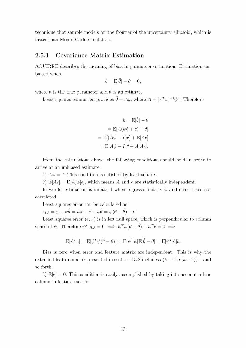
2.5.1 Covariance Matrix Estimation

AGUIRRE describes the meaning of bias in parameter estimation. Estimation un-

biased when

b = E[θ]− θ = 0,

where θ is the true parameter and θ is an estimate.

Least squares estimation provides θ = Ay, where A = [ψTψ]−1ψT . Therefore

b = E[θ]− θ

= E[A(ψθ + e)− θ]

= E[(Aψ − I)θ] + E[Ae]

= E[Aψ − I]θ + A[Ae].

From the calculations above, the following conditions should hold in order to

arrive at an unbiased estimate:

1) Aψ = I. This condition is satisfied by least squares.

2) E[Ae] = E[A]E[e], which means A and e are statistically independent.

In words, estimation is unbiased when regressor matrix ψ and error e are not

correlated.

Least squares error can be calculated as:

eLS = y − ψθ = ψθ + e− ψθ = ψ(θ − θ) + e.

Least squares error (eLS) is in left null space, which is perpendicular to column

space of ψ. Therefore ψT eLS = 0 =⇒ ψTψ(θ − θ) + ψT e = 0 =⇒

E[ψT e] = E[ψTψ(θ − θ)] = E[ψTψ]E[θ − θ] = E[ψTψ]b.

Bias is zero when error and feature matrix are independent. This is why the

extended feature matrix presented in section 2.3.2 includes e(k− 1), e(k− 2), ... and

so forth.

3) E[e] = 0. This condition is easily accomplished by taking into account a bias

column in feature matrix.

13

When estimation is unbiased, the covariance matrix can be estimated as follows:

cov[θ] = E[(θ − E[θ])(θ − E[θ])T ]

= E[(Ay − θ)(Ay − θ)T ]

= E[AyyTAT − AyθT − θyTAT + θθT ]

= E[A(ψθ + e)(ψθ + e)TAT − A(ψθ + e)θT − θ(ψθ + e)TAT + θθT ]

= E[(Aψθ + Ae)(Aψθ + Ae)T − (Aψθ + Ae)θT − θ(Aψθ + Ae)T + θθT ]

But Aψ = [ψTψ]−1ψTψ = I, then:

cov[θ] = E[(θ + Ae)(θ + Ae)T − (θ + Ae)θT − θ(θ + Ae)T + θθT ]

= E[AeeTAT ]

By assuming error as a white noise with variance σ2e :

cov[θ] = (ψTψ)−1σe2. (2.2)

2.5.2 Sampling on the boundary of the uncertainty ellipsoid

A proper ellipsoid in the n-dimensional space Rn centered at the origin may be

defined by the quadratic form

E = {x|xTΣ−1x = 1}, (2.3)

where Σ is the covariance matrix. Considering Σ to be the covariance matrix from a

Gaussian distribution, E in equation 2.3 is the boundary of the uncertainty ellipsoid

corresponding to σ = 1 standard deviation.

The covariance matrix is symmetric and can be written as

Σ = QDQT ,

where D is the diagonal matrix of eigenvalues of Σ and Q is the orthogonal matrix

of eigenvectors of Σ. Therefore

xT (QDQT )−1x = 1 =⇒ xTQD−1QTx = 1.

By choosing y = QTx,

yTD−1y = 1

14

impliesy2

1

λ1

+y2

2

λ2

+ ...+y2n

λn= 1,

where λi is the i-th eigenvalue of Σ.

Choosing ti = y2i ,

t1λ1

+t2λ2

+ ...+tnλn

= 1 (2.4)

In order to make left hand side of equation 2.4 equal to 1, ti = λivi, where

vi =kin∑i=1

ki

. For randomization purposes, ki is chosen from a uniform distribution

U [0, 1].

Therefore yi = ±√ti. The signal is chosen randomly between + and −.

Finally, for σ uncertainty level estimation, a sample on the ellipsoid of uncer-

tainties considering a Gaussian distribution centered at x with covariance matrix Σ

is

x = x+ σQy.

2.6 Online Learning

In this section, we will present the recursive least squares algorithm, which provides

an adaptive method in which parameter estimates are updated as new data become

available. This algorithm is suitable for reservoir identification problem because

the reservoir dynamics is time varying, especially when water or gas breakthrough

occurs.

In this work, we will explore import aspects of RLS filter, such as forgetting

factor and the choice of initial condition, as well as its mathematical formulation.

2.6.1 Recursive Least Squares

Given a model structure, the least squares pseudo inverse parameter estimate is

θ = (ψTψ)−1ψTy. (2.5)

We define

P = (ψTψ)−1. (2.6)

15

From pseudo inverse solution in equation 2.5, where ψi−1 represents i-th row of

the matrix ψ.

θk = Pk

k∑i=1

ψTi−1yi = Pk

k−1∑i=1

ψTi−1yi + PkψTk−1yk. (2.7)

For instant k − 1,

θk−1 = Pk−1

k−1∑i=1

ψTi−1yi =⇒k−1∑i=1

ψTi−1yi = P−1k−1θk−1. (2.8)

From the definition of matrix P in equation 2.6,

Pk = [k∑i=1

ψTi−1ψi−1]−1 (2.9)

P−1k =

k−1∑i=1

ψTi−1ψi−1 + ψTk−1ψk−1 (2.10)

= P−1k−1 + ψTk−1ψk−1. (2.11)

Combining equations 2.7 and 2.8,

θk = Pk[P−1k−1θk−1 + ψTk−1yk]. (2.12)

From equations 2.12 and 2.11,

θk = Pk(P−1k − ψ

Tk−1ψk−1)θk−1 + Pkψ

Tk−1yk (2.13)

= θk−1 + PkψTk−1(yk − ψk−1θk−1) (2.14)

The gain matrix is defined as

Kk = PkψTk−1 (2.15)

and the innovation at instant k is defined as

ηk = yk − ψk−1θk−1. (2.16)

The calculation of Pk still requires one matrix inversion at every algorithm iter-

16

ation. This can be avoided by using the inversion lemma

(A+BCD)−1 = A−1 − A−1B(C−1 +DA−1B)−1DA−1,

with

A = P−1k−1, B = ψTk−1, C = I,D = ψk−1,

and equation 2.11, P can be written as:

Pk = Pk−1 − Pk−1ψTk−1(ψk−1Pk−1ψ

Tk−1 + 1)−1ψk−1Pk−1. (2.17)

The gain matrix is calculated combining equations 2.15 and 2.17,

Kk =Pk−1ψ

Tk−1

ψk−1Pk−1ψTk−1 + 1

To sum up, the RLS algorithm can be implemented recursively

Kk =Pk−1ψ

Tk−1

ψk−1Pk−1ψTk−1 + 1

θk = θk−1 +Kk(yk − ψkθk−1)

Pk = Pk−1 −Kkψk−1Pk−1.

Furthermore, it is possible to give more importance to more recent data by using

a forgetting factor λ. In this case, instead of regular least squares, a weighted least

squares problem is solved.

The objective function to be minimized isk∑i=0

[(yi − ψi−1θ]2λk−i, with λ ≤ 1,

typically between 0.95 and 1. If λ = 1, regular least squares is solved and all

measured data have same importance. The lower λ is, the greater the weight given

to more recent data, which means that past data is “forgotten” faster.

It is important to mention that depending on the choice of the forgetting factor,

the filter may diverge. There is a trade-off between quick adaptation and filter

convergence. A suitable forgetting factor level is chosen by comparing forecast match

with real data.

The innovation ηk (equation 2.16) represents how fast parameters may change.

If innovation is zero, filter does not adapt. On the other hand, if the dynamical

system is no longer able to predict future correctly due to a change in dynamics,

the RLS algorithm with forgetting factor provides an adaptive filter which aims to

17

learn from new data.

RLS with forgetting factor (λ) algorithm can be implemented recursively:

Kk =Pk−1ψ

Tk−1

ψk−1Pk−1ψTk−1 + λ

θk = θk−1 +Kk(yk − ψkθk−1)

Pk =1

λ(Pk−1 −

Pk−1ψTk−1ψk−1Pk−1

ψk−1Pk−1ψTk−1 + λ)

If no prior information is known, a standard choice is θ = 0 and P = 10kI, where

I is the identity matrix and 3 ≤ k ≤ 7.

2.6.2 Practical Remarks about the Prior Knowledge in the

RLS filters

If prior information, such as a reservoir simulation result is known, model selection

procedure discussed previously can be used to define the model structure as well as

the initial condition for the RLS filter. This is a means by which prior knowledge

in an adaptive framework is able to provide physical aspects for the filter.

Prior knowledge can consider similarities between wells. In case of lack of infor-

mation from reservoir simulator, a similar well history data may provide an initial

condition guess for RLS filter.

2.7 Simulator-based identification and validation

of reservoir models

We analyze the “Two Flow Model” reservoir simulator, developed by Emerick [20],

in which there are 6 water injectors and 2 liquid producers.

Figure 2.4 depicts, in log scale, permeability distribution across reservoir cell

grids. In fact, this is a realization of a prior model in which the prior covariance

matrix follows a spherical covariance function.

There are two important connections, in which it is possible to notice a preferen-

tial path from injector 1 to producers 2 and 3, and another high permeability path

from injector 2 to producers 4 and 5.

This case study aims to check whether system identification procedure can be

successfully implemented in terms of capturing geological aspects, such as high per-

meability preferential paths. Moreover, we want to establish models that are suitable

for forecasting and assess them in independent test sets.

18

0 50 100 150 200 250 300

months

1500

2000

2500INJ-01 Water Injection Rate (bbl/day)

0 50 100 150 200 250 300

months

1500

2000

2500INJ-02 Water Injection Rate (bbl/day)

Figure 2.2: Water Injection Rates PRBS Excitation for System Identification. TheLiquid Producer Rates are kept constant.

2.7.1 Choice of Features and Experimental Design

In this experimental identification design, Liquid Producer Rates are kept constant,

while injection rates varies according to Table 2.1. PRBS (pseudo random binary

sequence) excitation is applied in injectors, depicted in Figure 2.2.

Table 2.1: Range of perturbation

Well MIN MAX

INJ-01 1500 2500INJ-02 1500 2500PRO-01 400 400PRO-02 700 700PRO-03 700 700PRO-04 700 700PRO-05 700 700PRO-06 400 400

We could consider, as possible choices of features, meaningful outputs such as

BHP (bottom hole pressure), WC (water cut) and Oil Rate as functions of water

injection rates, which were chosen as PRBS excitations. BHP could be analysed as

output, given that liquid production rate in simulation is constant and BHP reflects

block pressure variation, as depicted in Figure 1.1.

Another possibility is to assess water cut evolution and its correlations to water

19

Figure 2.3: Water saturation map is represented during 14 years. It is worthwhilepointing out the time variant characteristics of the production system, which variesespecially when water breakthrough occurs.

injection rates. Liquid Production Rate could be an interesting alternative choice

if BHP of producer wells were held constant, as chosen in Figure 1.2, but in this

case study the liquid production is chosen as a bias, since it is held constant in the

simulations.

Figure 2.3 depicts water saturation evolution in the reservoir for a 14 years

period. In 3 years, we can observe water breakthrough first in wells 2, 3 and 5

and subquently in wells 4, 6 and 1. Many of the examples in this chapter aim to

show how effective polynomial ARX and ARMAX representations can be in terms

of making predictions.

2.7.2 Results of ARX and ARMAX modeling

PRO-01 In this well, we will consider as output PRO-01 bottom hole pressure.

The features includes water injection rates (for both injector wells) and liquid pro-

duction rate (for producer PRO-01), which is bias in this case study.

The time window for analysis ranges from month 170 to 200, which means that,

for a total period of 30 months, 60% of data is used for training, 20% for validation

and 20% for test.

Figure 2.5 depicts training and validation results. 10 coefficients are used and

20

Figure 2.4: Reference log-permeability field, making evident the permeability pathconnectivity between INJ-01 and PRO-02/PRO-03 and INJ-02 and PRO-04/PRO-05.

0 5 10 15 20

time - months

5000

5100

5200

5300

5400

5500

5600

5700

BH

P (

psi)

Training Set

ARX ModelData Used for Training

1 2 3 4 5 6

time - months

5630

5640

5650

5660

5670

5680

5690

5700

5710

5720

5730

BH

P (

psi)

Validation Set - Forecast

ARX ModelData Used for Validation

Figure 2.5: Model Structure choice based on the Validation Set for the producerwell PRO-01.

21

0 5 10 15 20 25

time - months

5000

5100

5200

5300

5400

5500

5600

5700

5800

BH

P (

psi)

Training and Validation Data Set

Data Used for TrainingARX Model

0 5 10 15 20

Lag

-0.5

0

0.5

1

Sa

mp

le A

uto

co

rre

latio

n

Final Hypothesis ACF

Figure 2.6: Chosen the model structure, training and validation data set are used fortraining. Residual analysis indicates that the error is a white noise for the producerwell PRO-01.

ARX model structure is na = 3, nb = [1, 3, 3], nk = [0, 0, 0]. Once the ARX structure

has been defined, training and validation data are used for parameter estimation

and Figure 2.6 shows the results of a simulated model, which are quite similar to

training data set. ACF suggests, from residual analysis, that one step ahead error

is white noise. In other words, ACF means that ARX model captures all linear

correlations in the data.

Uncertainty estimation analysis reveals little uncertainty with respect to the

estimated parameters and, indeed, test dataset results lie within the range of uncer-

tainty of model prediction. Uncertainty ellipsoid considering 3 standard deviation

with 50 perturbations, shown in Figure 2.7, in month 200 ranges from 6125 to 6150

psi and real data corresponds to 6141 psi, an error smaller than 0.05% compared to

simulated forecast. Monte Carlo analysis also presents little uncertainty with 3000

simulations and test dataset is bounded by P-40 and P-60 curves. In this work,

P-x denotes a measure indicating the value above which a given percentage (x) of

observations in a group of observations falls.

With regards to step response analysis, as depicted in Figure 2.9, positive slope

for the average case in step response for both injectors suggests that they provoke

bottom hole pressure increase. In fact, this should be expected, since block pressure

increases and liquid rate is kept constant in simulation. Interestingly, step response

22

25 26 27 28 29 30 31

time - months

5750

5800

5850

5900

5950

6000

6050

6100

6150

6200

BH

P (

psi)

Ellipsoid of Uncertainty - sigma = 3, 50 perturbations

On the ellipsoid boundaryForecastTest Data Set

Figure 2.7: Test set assessment comparing the forecast on the average case (inblack) and Test Data Set. In green, 50 different parameter vectors with the samemodel structure were sampled on the Ellipsoid of Uncertainty considering 3 standarddeviation for the producer PRO-01.

25 26 27 28 29 30 31

time - months

5750

5800

5850

5900

5950

6000

6050

6100

6150

BH

P (

psi)

Monte Carlo Simulation - 3000 simulations

Test Data SetForecastP-10P-40P-60P-90

Figure 2.8: Instead of sampling on the ellipsoid of uncertainty, Monte Carlo simu-lation is performed. The curves P-10, P-40, P-60 and P-90 are defined with 3000simulations for the producer well PRO-01.

23

0 500 1000 1500 2000 2500 3000

time - months

-50

0

50

100

150

200

BH

P (

psi)

Injector 01

Average CaseUpper Uncertainty BoundLower Uncertainty Bound

0 500 1000 1500 2000 2500 3000

time - months

-50

0

50

100

150

200

BH

P (

psi)

Injector 02


0 500 1000 1500 2000 2500 3000

time - months

-50

0

50

100

150

200

BH

P (

psi)

Injector 01


0 500 1000 1500 2000 2500 3000

time - months

-50

0

50

100

150

200

BH

P (

psi)

Injector 02


Figure 2.9: Step Response: BHP - PRO-01. Both INJ-01 and INJ-02 contribute forBHP increase for the producer well PRO-01 in the step response.

suggests little difference from injector 1 to 2, even though injector 1 is located closer

to producer 1.

PRO-02 A period from month 40 to 140 is chosen for data analysis, where water

cut ranges from 40% to 93%. Training, validation and test set are distributed

according to 60%, 20% and 20%. Exogenous components are water injection rates,

liquid rate (bias) and output is water cut.

Figures 2.4 and 2.3 show a strong correlation between water cut in well 2 and

water injection rate from injector 1. The Water Saturation Map (Figure 2.3) shows

how the water front propagates spatiotemporally from the injector wells towards the

producer wells. The waterfront spatial propagation follows the permeability map

(Figure 2.4) of the grid. Each block in the grid has a permeability value indicated

by the corresponding color in the heat map in Figure 2.4. The preferential paths

have higher permeability values (towards the red end of the spectrum). We would

like to assess whether step response captures the correlation between water cut in

well 2 and water injection rate from injector 1.

Figure 2.10 depicts training and validation results for ARX model. The structure

which minimizes the error in the validation test is na = 2, nb = [1, 2, 3] and nk =

24

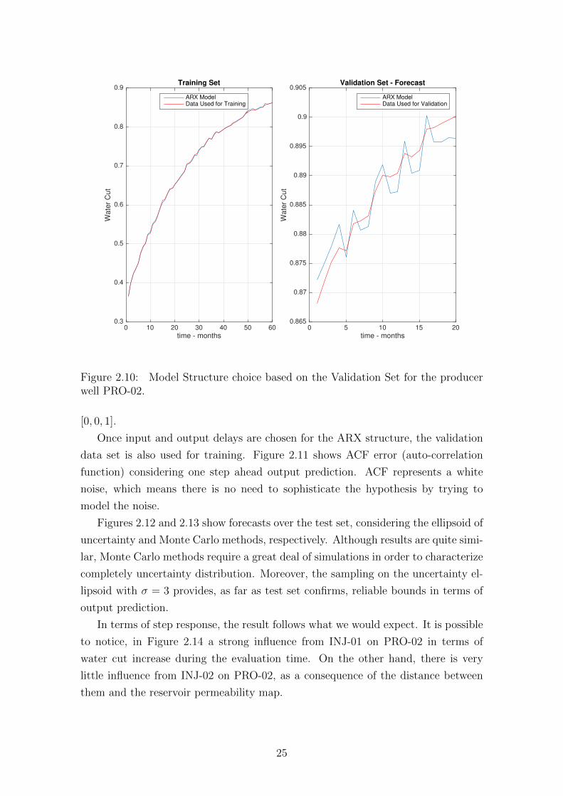
0 10 20 30 40 50 60

time - months

0.3

0.4

0.5

0.6

0.7

0.8

0.9

Wa

ter

Cu

t

Training Set

ARX ModelData Used for Training

0 5 10 15 20

time - months

0.865

0.87

0.875

0.88

0.885

0.89

0.895

0.9

0.905

Wa

ter

Cu

t

Validation Set - Forecast

ARX ModelData Used for Validation

Figure 2.10: Model Structure choice based on the Validation Set for the producerwell PRO-02.

[0, 0, 1].

Once input and output delays are chosen for the ARX structure, the validation

data set is also used for training. Figure 2.11 shows ACF error (auto-correlation

function) considering one step ahead output prediction. ACF represents a white

noise, which means there is no need to sophisticate the hypothesis by trying to

model the noise.

Figures 2.12 and 2.13 show forecasts over the test set, considering the ellipsoid of

uncertainty and Monte Carlo methods, respectively. Although results are quite simi-

lar, Monte Carlo methods require a great deal of simulations in order to characterize

completely uncertainty distribution. Moreover, the sampling on the uncertainty el-

lipsoid with σ = 3 provides, as far as test set confirms, reliable bounds in terms of

output prediction.

In terms of step response, the result follows what we would expect. It is possible

to notice, in Figure 2.14 a strong influence from INJ-01 on PRO-02 in terms of

water cut increase during the evaluation time. On the other hand, there is very

little influence from INJ-02 on PRO-02, as a consequence of the distance between

them and the reservoir permeability map.

25

0 20 40 60 80

time - months

0.3

0.4

0.5

0.6

0.7

0.8

0.9

1

Wa

ter

Cu

t



0 5 10 15 20

Lag

-0.4

-0.2

0

0.2

0.4

0.6

0.8

1

Sa

mp

le A

uto

co

rre

latio

n


Figure 2.11: Chosen the model structure, training and validation data set are usedfor training. Residual analysis indicates that the error is not very different from awhite noise for the producer well PRO-02.

82 84 86 88 90 92 94 96 98 100

time - months

0.9

0.905

0.91

0.915

0.92

0.925

0.93

0.935

0.94

Wa

ter

Cu

t



Figure 2.12: Test set assessment comparing the forecast on the average case (inblack) and Test Data Set. In green, 50 different parameter vectors with the samemodel structure were sampled on the Ellipsoid of Uncertainty considering 3 standarddeviation for the producer well PRO-02. It is worthwhile mentioning the scale, whichranges from 0.90 to 0.94, indicating a good agreement between the uncertaintyanalysis forecast and the test data set.

26

82 84 86 88 90 92 94 96 98 100

time - months

0.9

0.905

0.91

0.915

0.92

0.925

0.93

0.935W

ate

r C

ut

Monte Carlo Simulation - 3000 simulations

Test Data Set

Forecast

P-10

P-40

P-60

P-90

Figure 2.13: Instead of sampling on the ellipsoid of uncertainty, Monte Carlo sim-ulation is performed. The curves P-10, P-40, P-60 and P-90 are defined with 3000simulations for the producer PRO-02.

0 50 100 150 200

time - months

0

1

2

3

4

5

6

7

8

9

Wa

ter

Cu

t

×10-5 Injector 01


0 50 100 150 200

time - months

-3

-2

-1

0

1

2

3

Wa

ter

Cu

t

×10-5 Injector 02


Figure 2.14: Step Response for the producer wel PRO-02. INJ-01 has a meaningfulcontribution for water cut increase in PRO-02, whereas INJ-02 seems to have verylittle influence.

27

0 100 200 300

time - months

0

0.2

0.4

0.6

0.8

1

Wa

ter

Cu

t

Forgetting Factor = 0.990000

Original Time Series

0 100 200 300

time - months

-0.06

-0.04

-0.02

0

0.02

0.04

0.06

0.08

Pre

dic

tio

n E

rro

r

0 100 200 300

time - months

0

0.2

0.4

0.6

0.8

1

Wa

ter

Cu

t



0 100 200 300

time - months

-0.06

-0.04

-0.02

0

0.02

0.04

0.06

0.08

Pre

dic

tio

n E

rro

r

0 100 200 300

time - months

0

0.2

0.4

0.6

0.8

1

Wa

ter

Cu

t



0 100 200 300

time - months

-0.06

-0.04

-0.02

0

0.02

0.04

0.06

0.08

Pre

dic

tio

n E

rro

r

Figure 2.15: The graph shows 3 different choices for forgetting factors in the RLSfilter. 12 months ahead prediction of water cut for the producer PRO-03 (in blue)is compared with the original time series, which comes from the model simulation.

PRO-03: Water Cut - Recursive Least Squares In this case study, we want

to evaluate the performance of recursive least squares when it comes to adapting

and forecasting. After considering different structures for this case study, we choose

one that is simple enough to provide acceptable results in terms of both prediction

accuracy and meaningful interpretation of the exogenous components. We choose

na = 2, nb = [1, 2, 2], nk = [0, 0, 0] considering liquid rate (bias) and water injection

rates, respectively, as input features, and water cut as output.

Figure 2.15 shows 12 months ahead prediction in blue circle markers for three

different levels of forgetting factors: 0.990, 0.995 and 0.999. Initial condition for well

3 comes from the use of RLS during the whole period for well 4. This procedure

avoids reuse of well 3 data to adjust parameters for well 3, which would be un-

fair. Additionally, this provides a realistic initial condition for well 3 based on the

hypothesis that well 3 and 4 are close to each other.

Parameters adapt more when water breakthrough occurs (at time 35 months),

which represents a significant change in well dynamics. This can be observed in

prediction error, which provokes a bigger adaptation gain. No big differences are

observed among forgetting factors, but it is possible to state that forgetting factor

= 0.990 tends to make parameters more adaptive.

Considering forgetting factor 0.999, Figure 2.16 indicates how adaptation can

28

0 50 100 150 200 250 300

-1.5

-1

-0.5

0

0.5

1

1.5

2×10

-5 Exogenous Parameters

INJ-01

INJ-02

Figure 2.16: RLS - Exogenous Parameters Adaptation for the producer PRO-03.Interestingly, we see a pattern change after the water breakthrough, which meansthe filter adapts quickly and is able to capture the real connectivity among the wells.

provide a physical insight about dynamics in reservoir. Before water breakthrough,

water cut was zero and no additional information is available, which means pa-

rameters were close to initial condition. Indeed, it is possible to observe a high

permeability path between Injector-02 and Producer-04 in Figure 2.4.

At month 35, when water breakthrough occurs in well 3, water cut signal reveals

information about reservoir and we see change in the parameter pattern, which is

consistent from a physical viewpoint. In fact, from month 40 it is noticeable that

injector-01 contributes to watercut increase in this well because the sum of injector-

01 ARX parameters becomes and remains positive, whereas the sum of injector-02

ARX parameters becomes and remains negative, which suggests that injector-02 has

the opposite effect, namely, injector-02 increases oil production of well 3, which is

not an obvious conclusion a priori.

PRO-04: WC - Recursive Least Squares In this case study, we want to eval-

uate the evolution of parameters and their uncertainties while measured data is

assimilated. RLS algorithm is performed and forgetting factor is 0.999. Initially, we

considered a simple model structure (order two for both AR and exogenous compo-

nents), which led to a biased forecast result. To avoid the difficulty in considering

an adaptive model structure, we consider a more complex ARX model structure in

29

0 50 100 150 200 250 300

time - months

0

0.5

1

1.5

Wa

ter

Cu

t

Forgetting Factor: 0.999


0 50 100 150 200 250 300

time - months

-0.03

-0.02

-0.01

0

0.01

0.02

Pre

dic

tio

n E

rro

r

Figure 2.17: 12 months ahead prediction of water cut for the producer PRO-04(in blue) is compared with the original time series, which comes from the modelsimulation. Bigger adaptation is observed when water breakthrough occurs.

which the parameters change in the RLS filter algorithm and the structure is fixed

as na = 8, nb = [1, 8, 8] and nk = [0, 0, 0]. This means that the first regressor is the

liquid production rate (bias) and the others correspond to injection rates. We start

from standard RLS initial condition, θ = 0 and P = 103I, where I is the identity

matrix.

Figure 2.17 illustrates 12 months ahead prediction. Unlike the previous case, it is

worthwhile mentioning that no prior information about the well is considered, only

standard filter initial conditions. Prediction error graph indicates bigger adaptation

when water breakthrough occurs.

Furthermore, Figure 2.18 presents the sum of exogenous parameters for each

well. This graph suggests that INJ-02 has an important role regarding water cut

increase in PRO-04.

PRO-05: BHP - ARX and ARMAX comparison So far, we have shown how

effective ARX structure can be in terms of modeling and forecasting. We would like

to investigate the benefits of considering ARMAX structure when residual analysis

presents some indication that error could be modeled by a moving average filter.

From training and validation model selection previously presented in other cases,

and considering BHP data from month 150 to 300, we find an ARX structure

30

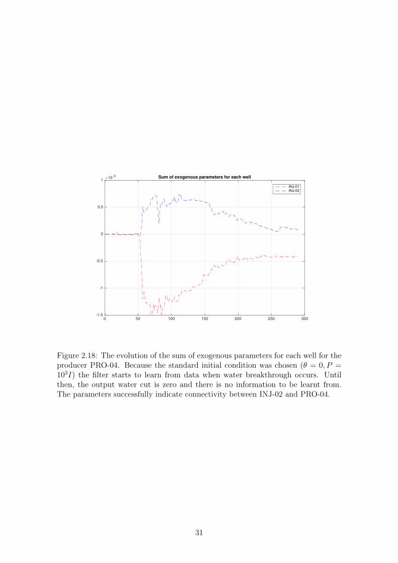
0 50 100 150 200 250 300

-1.5

-1

-0.5

0

0.5

1×10

-5 Sum of exogenous parameters for each well

INJ-01

INJ-02

Figure 2.18: The evolution of the sum of exogenous parameters for each well for theproducer PRO-04. Because the standard initial condition was chosen (θ = 0, P =103I) the filter starts to learn from data when water breakthrough occurs. Untilthen, the output water cut is zero and there is no information to be learnt from.The parameters successfully indicate connectivity between INJ-02 and PRO-04.

31

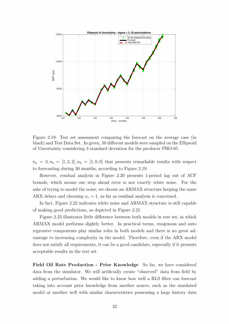
120 125 130 135 140 145 150 155

time - months

9000

9500

10000

10500

BH

P (

psi)



Figure 2.19: Test set assessment comparing the forecast on the average case (inblack) and Test Data Set. In green, 50 different models were sampled on the Ellipsoidof Uncertainty considering 3 standard deviation for the producer PRO-05.

na = 3, nb = [1, 2, 2], nk = [1, 0, 0] that presents remarkable results with respect

to forecasting during 30 months, according to Figure 2.19.

However, residual analysis in Figure 2.20 presents 1-period lag out of ACF

bounds, which means one step ahead error is not exactly white noise. For the

sake of trying to model the noise, we choose an ARMAX structure keeping the same

ARX delays and choosing nc = 1, as far as residual analysis is concerned.

In fact, Figure 2.22 indicates white noise and ARMAX structure is still capable

of making good predictions, as depicted in Figure 2.21.

Figure 2.23 illustrates little difference between both models in test set, in which

ARMAX model performs slightly better. In practical terms, exogenous and auto

regressive components play similar roles in both models and there is no great ad-

vantage to increasing complexity in the model. Therefore, even if the ARX model

does not satisfy all requirements, it can be a good candidate, especially if it presents

acceptable results in the test set.

Field Oil Rate Production - Prior Knowledge So far, we have considered

data from the simulator. We will artificially create “observed” data from field by

adding a perturbation. We would like to know how well a RLS filter can forecast

taking into account prior knowledge from another source, such as the simulated

model or another well with similar characteristics possessing a large history data

32

0 20 40 60 80 100 120

time - months

5000

5500

6000

6500

7000

7500

8000

8500

9000

9500

BH

P (

psi)



0 5 10 15 20

Lag

-0.4

-0.2

0

0.2

0.4

0.6

0.8

1

Sa

mp

le A

uto

co

rre

latio

n


Figure 2.20: Residual analysis indicates 1-period lag out of ACF bounds, whichsuggests that error could be modeled with a moving average (MA) component. Thisis why we attempt to model it evolving from ARX structure to ARMAX.

set.

Figure 2.24 shows initially estimated oil rate, in red using prior information

that could come from reservoir simulation, for instance. The blue curve represents

observed data, which RLS filter will attempt to match.

Prior knowledge curve provides initial condition for RLS filter. We will compare

the effect of choosing a prior initial condition with a standard RLS initial condition

(θ = 0, P = 103I).

Comparing Figures 2.26 and 2.25, both using forgetting factor = 0.999, na =

[2], nb = [1, 2, 2], nk = [0, 0, 0], the curve using an initial condition coming from data

assimilation of a prior knowledge data set presents little difficulty in adapting when

water cut is no longer zero, which happens when Field Oil Rate starts to decrease.

Even though RLS filter with standard initial condition filter (θ = 0, P = 103I)

does not adapt with ease, from month 100 ahead, 1 year ahead predictions present

little mismatch with observed data. Therefore, this case study suggests that a prior

knowledge information which provides an initial choice of the RLS parameters helps

to boost the filter convergence, showing better forecast results, mostly when water

breakthrough occurs.

33

120 125 130 135 140 145 150 155

time - months

9000

9500

10000

10500

BH

P (

psi)



Figure 2.21: Test set assessment comparing the forecast on the average case (inblack) and Test Data Set. In green, 50 different models were sampled on the Ellipsoidof Uncertainty considering 3 standard deviation for the producer PRO-05 using theARMAX model.

0 20 40 60 80 100 120

time - months

5000

5500

6000

6500

7000

7500

8000

8500

9000

9500

BH

P (

psi)


Data Used for TrainingARMAX Model

0 5 10 15 20

Lag

-0.2

0

0.2

0.4

0.6

0.8

1

Sa

mp

le A

uto

co

rre

latio

n


Figure 2.22: In fact, ARMAX model presents suitable results in residual analysis,which means choosing nc = 1 successfully models the error.

34

120 130 140 150 160

time - months

-2

0

2

4

6

8

10

BH

P (

psi)

ARX errorARMAX error

120 130 140 150 160

time - months

-0.02

0

0.02

0.04

0.06

0.08

0.1

0.12

Re

lative

Err

or

(%)

ARX errorARMAX error

Figure 2.23: Comparison between ARX and ARMAX in the test data set. Despiteits advantage of modeling the error, ARMAX presents results very similar to ARXin free simulation in the test data set.

0 50 100 150 200 250 300

time - months

0

500

1000

1500

2000

2500

3000

3500

4000

4500

BP

D

Field Oil Rate

Observed DataPrior Knowledge

Figure 2.24: Observed Data and Prior Knowledge Data Set. Prior Knowledge maycome from different sources, such as a numerical model reservoir simulation or an-other well with a large history data set with similar characteristics.

35

0 50 100 150 200 250 300

time - months

0

500

1000

1500

2000

2500

3000

3500

4000

4500F

ield

Oil

Ra

te (

BP

D)



0 50 100 150 200 250 300

time - months

-60

-40

-20

0

20

40

60

Pre

dic

tio

n E

rro

r

Figure 2.25: 12 months ahead prediction of the Field Oil Rate considering StandardRLS filter Initial Condition (θ = 0, P = 103I).

0 50 100 150 200 250 300

time - months

0

500

1000

1500

2000

2500

3000

3500

4000

4500

Fie

ld O

il R

ate

(B

PD

)



0 50 100 150 200 250 300

time - months

-80

-60

-40

-20

0

20

40

60

Pre

dic

tio

n E

rro

r

Figure 2.26: 12 months ahead prediction of the Field Oil Rate considering InitialCondition from data assimilation of a prior knowledge data set, as depicted in 2.24.

36

Chapter 3

Proxy States Based Model

While the previous chapter dealt with input-ouput models, this chapter will consider

state space models. In the reservoir problem, states are not effectively measured and

although they represent an abstraction from modeling perspective, in fact, they are

grid block properties which evolve during the simulation.

This dissertation deals with a two phase simulation, whose states are water sat-

uration and block pressure. The objective of this chapter is to explore the method

of snapshots in order to create a proxy model by using principal component anal-

ysis, which aims to reduce dimensionality such that system identification can be

performed with more ease.

To a certain extent, unlike linear transfer function representations, proxy states

based models represent physical aspects, such as geometry and geology characteris-

tics, by learning from a simulated model and its main features.

Furthermore, by making use of the linear state space proxy model obtained from

system identification procedures, we aim to perform optimization such that the NPV

(net present value) is maximized.

3.1 Method of snapshots

PINNAU [21] presents the method of snapshots, which represents trajectories of a

dynamical system at discrete time events. For time steps t1, t2, ..., tm, the snapshot

matrix X ∈ Rn×m is written as:

X = (x1, x2, ..., xm),

where xi = x(ti) ∈ Rn.

State dimension n is expected to be larger than the number of snapshots m.

Reservoir dynamics present slow evolution, which does not require snapshots at

high frequency, whereas n can be in the order of millions.

37

Proper orthogonal decomposition (POD) solves the problem of finding an or-

thogonal basis which contain as much information (or energy) as possible. In a

simple case, where POD basis dimension is one (k = 1), a direction w which retains

most information can be calculated by solving a constrained optimization problem:

maxw

m∑j=1

(xTj w)2

subject to wTw = 1.

Defining covariance matrix S =

∑j xjx

Tj

n− 1, assuming x is centered at zero, the

optimization problem can be stated as:

maxw

wTSw

subject to wTw = 1.

Lagrangian is L(w, λ) = wTSw + λ(1− wTw).

The gradient with respect to w is

∇w(L) = 2Sw − 2λw = 0.

Therefore Sw = λw, which means w is an eigenvector of the covariance matrix

S. The projected variance is wTSw = wTλw and its maximum value corresponds

to the largest eigenvalue. As a consequence, w is the eigenvector corresponding to

the largest eigenvalue of S.

Moreover, w is the eigenvector corresponding to the greatest right-singular value

of X. By using SVD factorization,

X = UΣV T ,

covariance matrix eigenvectors correspond to the columns of U.

For POD-basis with k > 1, we iterate this procedure and derive that wi(i =

2, ..., k) solves

maxwi

m∑j=1

(xTj wi)2

subject to wTi wi = 1 and wTi ws = 0 for all s ≤ i.

Therefore POD-basis with dimension k corresponds to the first k columns of

matrix U , from the singular value decomposition of X. Denoting the reduced matrix

Ur = U [:, 1 : k] in Matlab notation, a vector z in a reduced dimension is calculated

projecting the array x onto the column space of Ur:

38

z = UTr x

and x can be reconstructed as a linear combination of the POD-basis as follows:

x = Urz.

3.2 Relation between Regularization and PCA

This section briefly recalls the connection between dimensionality reduction using

principal component analysis and its regularization effect.

The least squares solution, with regularization parameter (α > 0), for the linear

system Ax = b (with no assumptions on A) is:

(αI + ATA)x = AT b.

Using singular value decomposition, A = UΣV T .

(αI + V ΣTUTUΣV T )x = V ΣTUT b.

V (αI + ΣTΣ)V T x = V ΣTUT b.

V TV (αI + ΣTΣ)V T x = V TV ΣTUT b.

(αI + ΣTΣ)V T x = ΣTUT b.

Since (αI + ΣTΣ) is a diagonal matrix, and α is positive,

x = V (αI + ΣTΣ)−1ΣTUT b =Nr∑j=1

vjσju

Tj b

σ2j + α

,

where Nr is the rank of A. Observing that

vjσju

Tj b

σ2j + α

≈

0, if 0 ≈ σj � αvju

Tj b

σj, σj � α

(3.1)

It can be seen that the regularization parameter α has, in common with PCA

rank reduction, a similar effect of removing the smaller singular values. On the other

hand, larger singular values are left almost unchanged.

Intuitively speaking, this is why principal component analysis plays an important

role in preventing overfitting. In other words, PCA dimensionality gets rid of less

informative dimensions in order to help generalization.

In order to retain a percentage ε of the variance (or energy), the typical criterion

is to keep k largest singular values, such that∑kj=1 σj∑Nr

j=1 σj≤ ε ≤ 1. (3.2)

39

3.3 State Matrix Estimation

AGUIRRE [10] presents matrix estimation procedure of a discrete linear model

represented as:

x(k) = Ax(k − 1) +Bu(k) + e(k) (3.3)

where x(k) = [x1(k)x2(k)...xn(k)]T is the vector that represents state at time step

k, u(k) = [u1(k)u2(k)...ur(k)]T is the vector that represents controls at time step k

and e(k) = [e1(k)e2(k)...en(k)]T are the regression error for each state at time step

k.

This linear system can also be written as:

x(k) =[A B

](x(k − 1)

u(k − 1)

)= γTmT (k − 1)

x(k)T = m(k − 1)γ =[x(k − 1)T u(k − 1)T

](ATBT

)For N time steps:

xN =

x(1)T

x(2)T

...

x(N)T

=

m(0)

m(1)

...

m(N − 1)

γ = Mγ

γ =

(AT

BT

)is estimated by least squares:

γ ≈M †xN ,

where † denotes pseudo inverse solution.

Now we can combine dimensionality reduction with this linear state space iden-

tification procedure such that the matrices A and B are estimated using the vector

z(k) = UTr x(k) instead of x(k). The procedure is as follows:

1) Write snapshot matrix and perform principal component analysis: z = UTr x.

2) Estimate matrices A and B, such that

z(k) = Az(k − 1) +Bu(k − 1) (3.4)

3) Reconstruct the estimate of the original vector x = Urz.

Let Nx the dimension of state space, Nz the dimension of reduced space, Nu the

dimension of control space.

For N time steps, O =

x(1)T

x(2)T

...

x(N)T

represents measured data, whose length is

40

NxN . In original space, matrix A has N2x parameters and B has NxNu. That is,

number of parameters to be estimated is Nx(Nx +Nu).

Least Squares estimation would be appropriate to obtain a good fit ifNx(Nx+Nu)

is significantly smaller than NxN. However, the snapshot matrix X tends to be tall

and thin, which means there are many more states associated with every grid block

than meaningful snapshots.

Therefore, dimensionality reduction plays a key role in preventing overfitting in

the matrix estimation problem.

Moreover, computational aspects play a critical role. It could be computationally

very expensive to estimate matrices A and B in the original space. For instance, if

Nx = 106, there are more than 1012 parameters to be estimated, apart from the fact

that such a structure would be prone to overfitting.

3.3.1 Output Identification

So far, we have presented a procedure by which it is possible to estimate state

variables, such as water saturation and block pressure. However, these variables

are not measured and they represent an abstraction that comes from a simulation

model. What we really measure can be defined as output variables, such as oil,

water, gas rates and bottom hole pressure.

This section aims to describe a linear representation of outputs as a function of

reduced states and controls. This kind of representation runs the risk of being an

oversimplification because well flow models may be strongly non linear.

For instance, water cut in the “Two-phase-flow model” depends on relative per-

meability curve, which itself can be modeled by a non linear function of water

saturation. Moreover, depending on how many perforations exist in the well, it

might be necessary to consider pressure drop between perforations, which could

make modeling more complicated.

Despite all this, as a first approximation, we will attempt to describe the output

as a linear function of state and input, i.e.:

y(k) = Cz(k) +Du(k). (3.5)

The advantage of modeling the dynamical system as a linear system is the fact

that this will turn the optimization problem a LP (linear programming) problem,

as described in section 3.4. If we were to consider rigorously all complex nonlinear

modeling, it would not be possible to take advantage of efficient solvers for convex

problems as we do in the LP problem.

In other words, this is a linear approximation in the neighborhood of a given

control trajectory u. Similarly to what was described in Section 3.3, we aim to find

41

matrices C and D such that quadratic error is minimized.

For N time steps:y(1)T

y(2)T

...

y(N)T

=

z(1)Tu(1)T

z(2)Tu(2)T

...

z(N)Tu(N)T

(CT

DT

).

The least squares solution is

(CT

DT

)=

z(1)Tu(1)T

z(2)Tu(2)T

...

z(N)Tu(N)T

†

y(1)T

y(2)T

...

y(N)T

.

3.4 Proxy based Optimization

In previous sections, we established a procedure which fits a linear system, that

works as a proxy model around a specified trajectory control u.

This section reformulates the optimal control problem of maximizing the net

present value (the performance index) at the end of a given time horizon, subject

to the proxy model dynamics and additional constraints on the inputs, as a mathe-

matical programming problem. This is done by treating the net present value as the

objective function to be maximized, subject to the discrete time proxy model dynam-

ics, rewritten as a sequence of equality constraints over the entire horizon. Since the

net present value is a linear function of the outputs, the proxy dynamics are chosen

as linear and the input constraints are all linear, the mathematical programming

problem is actually a linear programming problem, which confers computational

efficiency and scalability to the reformulation.

Given a reference trajectory control u, around which a linear system was iden-

tified, the aim is to find an optimal trajectory control u around u such that NPV

is maximized. In order to state the problem, parameters and variables in the opti-

mization problem are first defined. The parameters in this problem are as follows:

j is the interest rate.

Op is the oil price (dollar per barrel).

Wc is the water treatment cost (dollar per barrel).

Ic is the water injection cost (dollar per barrel).

Qmax represents the total liquid capacity constraint.

umax and umin are operational bounds for the trajectory controls.

∆u represents the box constraint in which the proxy model could be valid around

u.

sr is the slew rate, which imposes softness in the trajectory control.

42

z0 is the initial condition in the reduced space after dimensionality reduction

procedure.

The variables up and ui corresponds to the controls in producers and injectors,

respectively. In this work, producers controls are liquid rate and injectors controls

are water injection rates.

The other variables in this problem are:

Qo(t) is the oil rate vector for all producer wells at time step t.

Qo,T (t) is the total oil production at time step t, defined in equation (3.9).

Qliq,T (t) is the total liquid production at time step t, defined in equation (3.10).

Qw,T (t) is the total water production at time step t, defined in equation (3.12).

Qinj,T (t) is the total injection rate at time step t, defined in equation (3.13).

The corresponding linear programming problem is formulated as follows:

maxup,ui

NPV =T∑t=1

Qo,T (t)Op −Qw,T (t)Wc −Qinj,T (t)Ic(1 + j)t

(3.6)

s.t. z(t+ 1) = Az(t) +Bu(t+ 1) t = 0, . . . , T − 1 (3.7)

Qo(t) = Cz(t) +Du(t) t = 1, . . . , T (3.8)

Qo,T (t) = 1TQo(t) t = 1, . . . , T (3.9)

Qliq,T (t) = 1Tup(t) t = 1, . . . , T (3.10)

u(t)T = [up(t)Tui(t)

T ] t = 1, . . . , T (3.11)

Qw,T (t) = Qliq,T (t)−Qo,T (t) t = 1, . . . , T (3.12)

Qinj,T (t) = 1Tui(t) t = 1, . . . , T (3.13)

Qliq,T (t) ≤ Qmax t = 1, . . . , T (3.14)

u(t)− u(t) ≤ ∆u t = 1, . . . , T (3.15)

u(t)− u(t) ≥ −∆u t = 1, . . . , T (3.16)

umin ≤ u(t) ≤ umax t = 1, . . . , T (3.17)

u(t+ 1)− u(t) ≥ −sr t = 0, . . . , T − 1 (3.18)

u(t+ 1)− u(t) ≤ sr t = 0, . . . , T − 1 (3.19)

z(0) = z0, (3.20)

This linear program as well as the decision time horizon will both scale linearly

with the number of wells being considered. Even so, this does not represent a big

challenge in terms of computing time because modern LP software easily handles

very large problems (millions of variables and constraints). In this dissertation,

which deals with a toy proof of concept problem, we solve it by using cvxpy [15],

a mathematical modeling language available in the Python environment for convex

43

problems.

Trust Region Method Due to the nonlinear nature of this optimization problem,

trust region methods (see CONN et al. [13]) represent a suitable technique in which

the proxy model from system identification can be used in optimization framework.

Algorithm 1 describes the optimization procedure. Given an initial condition

(u,∆u), a linear system is identified in this region and used as a proxy model for

a LP problem. This identification procedure, described in line 4 of algorithm 1,

takes into account PRBS (pseudo random binary sequence) excitation in the region

(u,∆u).

If the optimization result is consistent with simulation in terms of objective

function increase, the optimal control calculation is the new current point and,

depending on how well the proxy model can describe the system, the trust region

confidence region (∆u) may increase or decrease.

The proxy model may lack consistency, which means the simulation does not

show an increase in the objective function, whereas the proxy model says so. In

this case, ρ ≤ 0 and the algorithm 1 performs system identification in order to find

another suitable linear proxy model, more likely to represent the simulation around

the current trajectory control.

Finally, the algorithm stops if the maximum iteration is reached or the trust

region reduces to a region smaller than ∆min, which means the algorithm converged

towards an optimal solution.

3.5 Results

3.5.1 Assessment of Proxy Model

The objective of this section is to assess whether a surrogate (aka proxy) linear

model is suitable for optimization purposes.

Linear Model Identification Given an initial trajectory control u, we will per-

form system identification by using PRBS excitation in a region ∆u, using the reser-

voir model described in 2.4. More specifically, we will derive a linear dynamical

system, as described in Section 3.3.

Figure 3.1 depicts the PRBS excitation around the trajectory control

u(k) = [600, 2500, 2500, 2500, 2500, 750, 5675, 5675]T

with

∆u(k) = [50, 50, 50, 50, 50, 50, 50, 50]T

44

Algorithm 1 Adapted Trust Region algorithm

1: procedure Trust Region(u, ∆u) . initial condition2: iter ← 0 . iteration count initialization3: Evaluate f(u) . by using the simulation model4: Identify the linear model in the region (u,∆u) . as shown in Section 3.35: Evaluate linear proxy objective function f(u)6: Calculate u∗ by solving the optimization problem in the region (u,∆u) . as

shown in Section 3.47: Evaluate f(u∗) . by using the simulation model8: Evaluate linear proxy objective function f(u∗)

9: Calculate ρ = f(u∗)−f(u)

f(u∗)−f(u)

10: if ρ ≤ 0 then . proxy is not consistent11: ∆u ← 0.25∆u

12: go to line 413: end if14: if 0 ≤ ρ ≤ 0.25 then . we no longer trust the proxy model as before15: ∆u ← 0.25∆u

16: u← u∗

17: f(u)← f(u∗)18: end if19: if 0.25 ≤ ρ ≤ 0.75 then20: ∆u ← ∆u

21: u← u∗

22: f(u)← f(u∗)23: end if24: if ρ ≥ 0.75 then25: ∆u ← 2∆u

26: u← u∗

27: f(u)← f(u∗)28: end if29: iter ← iter + 130: if ∆u ≤ ∆min or iter > Nmax then31: break . stop criterion32: end if33: go to line 534: end procedure

45

550

575

600

625

650

BPD

PRO-01

2450

2475

2500

2525

2550

BPD

PRO-02

2450

2475

2500

2525

2550

BPD

PRO-03

2450

2475

2500

2525

2550

BPD

PRO-04

2450

2475

2500

2525

2550

BPD

PRO-05

700

725

750

775

800

BPD

PRO-06

5625

5650

5675

5700

5725

BPD

INJ-01

0 5 10 15 20 25 30 35 40time (month)

5625

5650

5675

5700

5725

BPD

INJ-02

Figure 3.1: Pseudo Random Binary Sequence (PRBS) Excitation considering bothproducer and injector wells. This graph represents LPR (liquid production rate) forall producer wells (from PRO-01 to PRO-06) and WIR (water injection rate) for allinjector wells (INJ-01 and INJ-02).

46

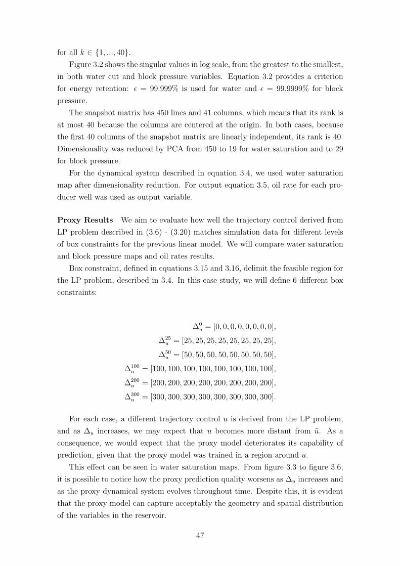
for all k ∈ {1, ..., 40}.Figure 3.2 shows the singular values in log scale, from the greatest to the smallest,

in both water cut and block pressure variables. Equation 3.2 provides a criterion

for energy retention: ε = 99.999% is used for water and ε = 99.9999% for block

pressure.

The snapshot matrix has 450 lines and 41 columns, which means that its rank is

at most 40 because the columns are centered at the origin. In both cases, because

the first 40 columns of the snapshot matrix are linearly independent, its rank is 40.

Dimensionality was reduced by PCA from 450 to 19 for water saturation and to 29

for block pressure.

For the dynamical system described in equation 3.4, we used water saturation

map after dimensionality reduction. For output equation 3.5, oil rate for each pro-

ducer well was used as output variable.

Proxy Results We aim to evaluate how well the trajectory control derived from

LP problem described in (3.6) - (3.20) matches simulation data for different levels

of box constraints for the previous linear model. We will compare water saturation

and block pressure maps and oil rates results.

Box constraint, defined in equations 3.15 and 3.16, delimit the feasible region for

the LP problem, described in 3.4. In this case study, we will define 6 different box

constraints:

∆0u = [0, 0, 0, 0, 0, 0, 0, 0],

∆25u = [25, 25, 25, 25, 25, 25, 25, 25],

∆50u = [50, 50, 50, 50, 50, 50, 50, 50],

∆100u = [100, 100, 100, 100, 100, 100, 100, 100],

∆200u = [200, 200, 200, 200, 200, 200, 200, 200],

∆300u = [300, 300, 300, 300, 300, 300, 300, 300].

For each case, a different trajectory control u is derived from the LP problem,

and as ∆u increases, we may expect that u becomes more distant from u. As a

consequence, we would expect that the proxy model deteriorates its capability of

prediction, given that the proxy model was trained in a region around u.

This effect can be seen in water saturation maps. From figure 3.3 to figure 3.6,

it is possible to notice how the proxy prediction quality worsens as ∆u increases and

as the proxy dynamical system evolves throughout time. Despite this, it is evident

that the proxy model can capture acceptably the geometry and spatial distribution

of the variables in the reservoir.

47

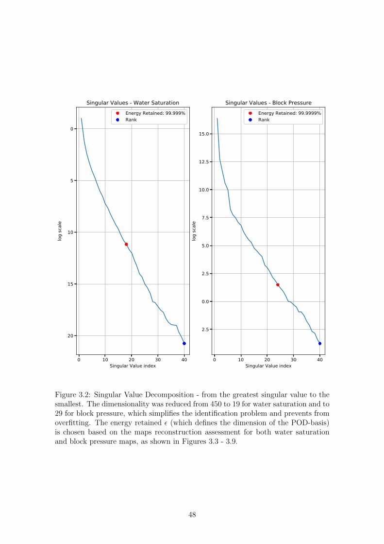
0 10 20 30 40Singular Value index

−20

−15

−10

−5

0

log scale

Singular Values - Water SaturationEnergy Retained: 99.999%Rank

0 10 20 30 40Singular Value index

−2.5

0.0

2.5

5.0

7.5

10.0

12.5

15.0

log scale

Singular Values - Block PressureEnergy Retained: 99.9999%Rank

Figure 3.2: Singular Value Decomposition - from the greatest singular value to thesmallest. The dimensionality was reduced from 450 to 19 for water saturation and to29 for block pressure, which simplifies the identification problem and prevents fromoverfitting. The energy retained ε (which defines the dimension of the POD-basis)is chosen based on the maps reconstruction assessment for both water saturationand block pressure maps, as shown in Figures 3.3 - 3.9.

48

0 months - proxy 10 months - proxy 20 months - proxy 30 months - proxy 40 months - proxy

0 months - simulated 10 months - simulated 20 months - simulated 30 months - simulated 40 months - simulated

0 months - difference (%) 10 months - difference (%) 20 months - difference (%) 30 months - difference (%) 40 months - difference (%)

0.0

0.2

0.4

0.6

0.8

1.0

0.0

0.2

0.4

0.6

0.8

1.0

0.0

0.2

0.4

0.6

0.8

1.0

0.0

0.2

0.4

0.6

0.8

1.0

0.0

0.2

0.4

0.6

0.8

1.0

0.0

0.2

0.4

0.6

0.8

1.0

0.0

0.2

0.4

0.6

0.8

1.0

0.0

0.2

0.4

0.6

0.8

1.0

0.0

0.2

0.4

0.6

0.8

1.0

0.0

0.2

0.4

0.6

0.8

1.0

0.00

0.01

0.02

0.03

0.04

0.05

0.00

0.01

0.02

0.03

0.04

0.05

0.00

0.01

0.02

0.03

0.04

0.05

0.00

0.01

0.02

0.03

0.04

0.05

0.00

0.01

0.02

0.03

0.04

0.05

Figure 3.3: The first row shows water saturation evolution according to the proxymodel, the second according to the simulated model and the last row shows thedifference between the two, for the case in which the box constraint allows zero(∆0

u) deviation from reference trajectory.

49




0.0

0.2

0.4

0.6

0.8

1.0

0.0

0.2

0.4

0.6

0.8

1.0

0.0

0.2

0.4

0.6

0.8

1.0

0.0

0.2

0.4

0.6

0.8

1.0

0.0

0.2

0.4

0.6

0.8

1.0

0.0

0.2

0.4

0.6

0.8

1.0

0.0

0.2

0.4

0.6

0.8

1.0

0.0

0.2

0.4

0.6

0.8

1.0

0.0

0.2

0.4

0.6

0.8

1.0

0.0

0.2

0.4

0.6

0.8

1.0

0.00

0.01

0.02

0.03

0.04

0.05

0.00

0.01

0.02

0.03

0.04

0.05

0.00

0.01

0.02

0.03

0.04

0.05

0.00

0.01

0.02

0.03

0.04

0.05

0.00

0.01

0.02

0.03

0.04

0.05

Figure 3.4: The first row shows water saturation evolution according to the proxymodel, the second according to the simulated model and the last row shows thedifference between the two, for the case in which the box constraint allows deviation±100 barrels per day (∆100

u ) from reference trajectory.

50




0.0

0.2

0.4

0.6

0.8

1.0

0.0

0.2

0.4

0.6

0.8

1.0

0.0

0.2

0.4

0.6

0.8

1.0

0.0

0.2

0.4

0.6

0.8

1.0

0.0

0.2

0.4

0.6

0.8

1.0

0.0

0.2

0.4

0.6

0.8

1.0

0.0

0.2

0.4

0.6

0.8

1.0

0.0

0.2

0.4

0.6

0.8

1.0

0.0

0.2

0.4

0.6

0.8

1.0

0.0

0.2

0.4

0.6

0.8

1.0

0.00

0.01

0.02

0.03

0.04

0.05

0.00

0.01

0.02

0.03

0.04

0.05

0.00

0.01

0.02

0.03

0.04

0.05

0.00

0.01

0.02

0.03

0.04

0.05

0.00

0.01

0.02

0.03

0.04

0.05



51




0.0

0.2

0.4

0.6

0.8

1.0

0.0

0.2

0.4

0.6

0.8

1.0

0.0

0.2

0.4

0.6

0.8

1.0

0.0

0.2

0.4

0.6

0.8

1.0

0.0

0.2

0.4

0.6

0.8

1.0

0.0

0.2

0.4

0.6

0.8

1.0

0.0

0.2

0.4

0.6

0.8

1.0

0.0

0.2

0.4

0.6

0.8

1.0

0.0

0.2

0.4

0.6

0.8

1.0

0.0

0.2

0.4

0.6

0.8

1.0

0.00

0.01

0.02

0.03

0.04

0.05

0.00

0.01

0.02

0.03

0.04

0.05

0.00

0.01

0.02

0.03

0.04

0.05

0.00

0.01

0.02

0.03

0.04

0.05

0.00

0.01

0.02

0.03

0.04

0.05



52

In figures 3.7 to figure 3.9, similar phenomena are observed for the block pressure

variable. It is worth pointing out that the block pressure variable presents more

difficulty to be explained by a linear model compared to water saturation variable,

and requires more energy to be retained. In fact, the block pressure map presents

bigger relative errors compared to water saturation ones. This may be due to the

fact that the total compressibility of the reservoir system is quite small, which causes

larger changes in dynamics in response to pressure changes.

Even though the proxy model was trained centered at u with amplitude ∆u =

[50, 50, 50, 50, 50, 50, 50, 50], as depicted in figure 3.1, for ∆100u , ∆200

u , ∆300u , the results

shown in figures 3.4, 3.5 and 3.6 for water saturation maps suggests good capability

of generalization. Unlike water saturation maps, block pressure maps do not perform

so well for deviations from the reference control trajectory larger than ±50 barrels

per day.

Figure 3.10 represents the case where u = u. In fact, this is the case where the

proxy model presents the best match with simulation results in terms of output

results, whereas from figure 3.11 to 3.13, we observe a slight deterioration in the

proxy performance.

Even though a linear proxy model is not completely able to represent all complex-

ity of the reservoir simulation, it is consistently able to indicate how the dynamical

system evolves. The Trust Region Algorithm 1 makes use of this capability in order

to handle the non linear problem as a sequence of linear problems.

53




2000

2250

2500

2750

3000

3250

3500

3750

4000

2000

2250

2500

2750

3000

3250

3500

3750

4000

2000

2250

2500

2750

3000

3250

3500

3750

4000

2000

2250

2500

2750

3000

3250

3500

3750

4000

2000

2250

2500

2750

3000

3250

3500

3750

4000

2000

2250

2500

2750

3000

3250

3500

3750

4000

2000

2250

2500

2750

3000

3250

3500

3750

4000

2000

2250

2500

2750

3000

3250

3500

3750

4000

2000

2250

2500

2750

3000

3250

3500

3750

4000

2000

2250

2500

2750

3000

3250

3500

3750

4000

0.00

0.01

0.02

0.03

0.04

0.05

0.00

0.01

0.02

0.03

0.04

0.05

0.00

0.01

0.02

0.03

0.04

0.05

0.00

0.01

0.02

0.03

0.04

0.05

0.00

0.01

0.02

0.03

0.04

0.05

Figure 3.7: The first row shows block pressure (in psi) evolution according to theproxy model, the second according to the simulated model and the last row showsthe difference between the two, for the case in which the box constraint allows zerodeviation (∆0

u) from reference trajectory.

54




2000

2250

2500

2750

3000

3250

3500

3750

4000

2000

2250

2500

2750

3000

3250

3500

3750

4000

2000

2250

2500

2750

3000

3250

3500

3750

4000

2000

2250

2500

2750

3000

3250

3500

3750

4000

2000

2250

2500

2750

3000

3250

3500

3750

4000

2000

2250

2500

2750

3000

3250

3500

3750

4000

2000

2250

2500

2750

3000

3250

3500

3750

4000

2000

2250

2500

2750

3000

3250

3500

3750

4000

2000

2250

2500

2750

3000

3250

3500

3750

4000

2000

2250

2500

2750

3000

3250

3500

3750

4000

0.00

0.01

0.02

0.03

0.04

0.05

0.00

0.01

0.02

0.03

0.04

0.05

0.00

0.01

0.02

0.03

0.04

0.05

0.00

0.01

0.02

0.03

0.04

0.05

0.00

0.01

0.02

0.03

0.04

0.05

Figure 3.8: The first row shows block pressure (in psi) evolution according to theproxy model, the second according to the simulated model and the last row showsthe difference between the two, for the case in which the box constraint allows adeviation of ±25 barrels per day (∆25


55




2000

2250

2500

2750

3000

3250

3500

3750

4000

2000

2250

2500

2750

3000

3250

3500

3750

4000

2000

2250

2500

2750

3000

3250

3500

3750

4000

2000

2250

2500

2750

3000

3250

3500

3750

4000

2000

2250

2500

2750

3000

3250

3500

3750

4000

2000

2250

2500

2750

3000

3250

3500

3750

4000

2000

2250

2500

2750

3000

3250

3500

3750

4000

2000

2250

2500

2750

3000

3250

3500

3750

4000

2000

2250

2500

2750

3000

3250

3500

3750

4000

2000

2250

2500

2750

3000

3250

3500

3750

4000

0.00

0.01

0.02

0.03

0.04

0.05

0.00

0.01

0.02

0.03

0.04

0.05

0.00

0.01

0.02

0.03

0.04

0.05

0.00

0.01

0.02

0.03

0.04

0.05

0.00

0.01

0.02

0.03

0.04

0.05

Figure 3.9: The first row shows block pressure (in psi) evolution according to theproxy model, the second according to the simulated model and the last row showsthe difference between the two, for the case in which the box constraint allows adeviation of ±50 barrels per day (∆50


56

time (month)0

200

400

600

800

1000

1200

BPD

PRO-01Output - ProxyOutput - SimulatedControl

time (month)0

500

1000

1500

2000

2500

3000

BPD

PRO-02

Output - ProxyOutput - SimulatedControl

time (month)0

500

1000

1500

2000

2500

3000

BPD

PRO-03


time (month)0

500

1000

1500

2000

2500

3000

BPD

PRO-04


time (month)0

500

1000

1500

2000

2500

3000

BPD

PRO-05


time (month)0

200

400

600

800

1000

BPD


0 5 10 15 20 25 30 35 40time (month)

5400

5600

5800

6000

BPD

INJ-01Control

0 5 10 15 20 25 30 35 40time (month)

5400

5600

5800

6000

BPD

INJ-02Control

Figure 3.10: For all producer wells, the output variable is oil production rate. Thefigure compares the output of the proxy model with the simulated one. In green, thecontrol (liquid production rate) resulted from the LP problem is shown in the casein which the box constraint allows zero deviation (∆0

u) from reference trajectory.

57

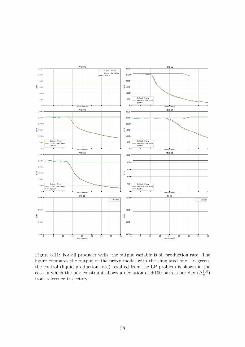
time (month)0

200

400

600

800

1000

1200

BPD


time (month)0

500

1000

1500

2000

2500

3000

BPD

PRO-02


time (month)0

500

1000

1500

2000

2500

3000

BPD

PRO-03


time (month)0

500

1000

1500

2000

2500

3000

BPD

PRO-04


time (month)0

500

1000

1500

2000

2500

3000

BPD

PRO-05


time (month)0

200

400

600

800

1000

BPD

PRO-06


0 5 10 15 20 25 30 35 40time (month)

5400

5600

5800

6000

BPD

INJ-01Control

0 5 10 15 20 25 30 35 40time (month)

5400

5600

5800

6000

BPD

INJ-02Control

Figure 3.11: For all producer wells, the output variable is oil production rate. Thefigure compares the output of the proxy model with the simulated one. In green,the control (liquid production rate) resulted from the LP problem is shown in thecase in which the box constraint allows a deviation of ±100 barrels per day (∆100

u )from reference trajectory.

58

time (month)0

200

400

600

800

1000

1200

BPD


time (month)0

500

1000

1500

2000

2500

3000

BPD

PRO-02


time (month)0

500

1000

1500

2000

2500

3000

BPD

PRO-03


time (month)0

500

1000

1500

2000

2500

3000

BPD

PRO-04


time (month)0

500

1000

1500

2000

2500

3000

BPD


time (month)0

200

400

600

800

1000

BPD

PRO-06


0 5 10 15 20 25 30 35 40time (month)

5400

5600

5800

6000

BPD

INJ-01Control

0 5 10 15 20 25 30 35 40time (month)

5400

5600

5800

6000

BPD

INJ-02Control


u )from reference trajectory.

59

time (month)0

200

400

600

800

1000

1200

BPD


time (month)0

500

1000

1500

2000

2500

3000

BPD

PRO-02


time (month)0

500

1000

1500

2000

2500

3000

BPD

PRO-03


time (month)0

500

1000

1500

2000

2500

3000

BPD

PRO-04


time (month)0

500

1000

1500

2000

2500

3000

BPD


time (month)0

200

400

600

800

1000

BPD


0 5 10 15 20 25 30 35 40time (month)

5400

5600

5800

6000

BPD

INJ-01

Control

0 5 10 15 20 25 30 35 40time (month)

5400

5600

5800

6000

BPD

INJ-02

Control


u )from reference trajectory. As the allowed deviation is larger, the proxy model tendsto present larger deviations from the simulation model.

60

3.5.2 Optimization Results

As previously discussed, we aim to maximize the Net Present Value (NPV) by choice

of the trajectory control. Table 3.1 presents the range chosen for each well: PRO-

01 and PRO-06 ranges are different from the others due to their locally smaller

permeability values.

The objective of this discussion is to present the results of the Trust Region

algorithm (algorithm 1), showing how the controls can vary according to different

capacity constraints (3.14).

The interest rate defined in this problem is 1% per month, Op is 80 dollars per

barrel, Wc is 10 dollar per barrel and Ic is zero. The slew rate (equation 3.18) is 50

BPD. Secondary controls (BHP bounds) are addressed internally in the simulation

model using a standard specification.

Table 3.1: Liquid Rate Bounds (BPD)

Well MIN MAX

PRO-01 500 1200PRO-02 2000 3000PRO-03 2000 3000PRO-04 2000 3000PRO-05 2000 3000PRO-06 500 1000INJ-01 5000 8000INJ-02 5000 8000

Let the initial condition be

u = [600, 2500, 2500, 2500, 2500, 750, 5675, 5675],

with liquid capacity constraint equals 11350 BPD. We start from an initial condition

respecting this constraint and we aim to find how liquid rates are balanced among

producer wells, as well as the injector trajectory controls.

Figure 3.14 shows a fast evolution of the net present value in the first 5 iterations.

The algorithm stopped due to the criterion ∆min = [10, 10, 10, 10, 10, 10, 10, 10],

which was reached in 15 iterations. The simulator was called 17 times: 15 times in

line 8 of algorithm 1 and 2 times in line 4, where system identification procedure

with PRBS excitation is performed.

NPV has increased by 9.10%, from 19.71 to 21.51 MM dollars. Cumulative oil

production at month 40 evolved from 9.04 to 9.80 MM of barrels, which means an

increase by 8.37% in the recovery factor.

Furthermore, the liquid capacity constraint is active during the whole period

considered, which makes the problem more interesting. In fact, the optimization

61

1 3 5 7 9 11 13 15iterations

590

600

610

620

630

640

MM dollars

Net Present Value (NPV)

0 5 10 15 20 25 30 35 40Time - months

0

2

4

6

8

10

MM

BBL

Cumulative Oil Production (NP)Initial ConditionSolution

0 5 10 15 20 25 30 35 40Time - months

10000

10500

11000

11500

12000

12500

BPD

Total Liquid Production RateLiquid Capacity Constraintsolution

0 5 10 15 20 25 30 35 40Time - months

10000

10500

11000

11500

12000

12500

BPD

Total Injection Ratesolution

Figure 3.14: The first graph shows the rapid initial increase of the NPV due to theoptimization algorithm achieving 9.1% overall gain. The second graph comparesoptimal cumulative oil production (blue curve) and initial solution (black curve).The third graph shows Total Liquid Production Rate attaining its upper bound(Liquid Capacity Constraint) and the fourth graph shows Total Injection Rate.

62

algorithm decides how to distribute the controls among the wells in order to optimize

the reservoir water front efficiency as a consequence of maximizing the NPV. An

important aspect of this methodology is to handle operational constraints in the

optimization problem itself, not internally in the simulator, which may result in

more significant gains.

Figures 3.15 and 3.16 show how the trajectory control evolves in the optimization

procedure. The solution found for the wells PRO-01 and PRO-06 are stuck in the

upper bound. This is quite reasonable due to the fact that their permeability are

smaller, which makes them less efficient in terms of fluid production.

The wells PRO-02 and PRO-05 present the optimized trajectory control with

smaller liquid rate control values than the initial one. This may be due to the

existence of a preferred permeability path, as can be seen in figure 2.4. Because of

this, figure 3.17 shows a breakthrough delay of 2 months for PRO-02 and PRO-05,

which is desirable. Henceforth, the term water breakthrough delay will be used to

refer to the delay in water breakthrough caused by the use of an optimal control.

Thus, larger water breakthrough delays represent gains in oil production.

The wells PRO-03 and PRO-04 seem to balance each other such that liquid

capacity constraint is reached. PRO-03 presents a smaller control value compared

to the initial condition, which delays the water breakthough by 3 months. On the

other hand, PRO-04 balances it and its water breakthrough occurs 4 months before

in the optimal case. In spite of this, most wells presented a larger breakthrough

delay in the improved case and their water cuts are kept smaller.

The injector wells respect an optional constraint, which was used in this work,

namely that total injection rate is bigger than total liquid production. Interestingly,

at time step 25, water injection in INJ-02 is increased, followed by a liquid production

rate increase in PRO-04, which presents the smallest water cut among all producer

wells of approximately 20%.

63

5 10 15 20 25 30 35 40

500

600

700

800

900

1000

1100

1200

BPD

LPR PRO-01iter 1iter 2iter 3iter 4iter 5iter 6iter 7iter 8iter 9iter 10iter 11iter 12iter 13iter 14iter 15upper boundlower bound

5 10 15 20 25 30 35 40

2000

2200

2400

2600

2800

3000

BPD


5 10 15 20 25 30 35 40Time - month

2000

2200

2400

2600

2800

3000

BPD


5 10 15 20 25 30 35 40Time - month

2000

2200

2400

2600

2800

3000

BPD


Figure 3.15: Figure shows the evolution of the trajectory controls (liquid productionrate for producers PRO-01, PRO-02, PRO-03 and PRO-04) for all iterations in thetrust region algorithm, from the initial condition (iter 1) to the final solution (iter15).

64

5 10 15 20 25 30 35 40

2000

2200

2400

2600

2800

3000

BPD


5 10 15 20 25 30 35 40

500

600

700

800

900

1000

BPD


5 10 15 20 25 30 35 40Time - month

5000

5500

6000

6500

7000

7500

8000

BPD

WIR INJ-01iter 1iter 2iter 3iter 4iter 5iter 6iter 7iter 8iter 9iter 10iter 11iter 12iter 13iter 14iter 15upper boundlower bound

5 10 15 20 25 30 35 40Time - month

5000

5500

6000

6500

7000

7500

8000

BPD

WIR INJ-02iter 1iter 2iter 3iter 4iter 5iter 6iter 7iter 8iter 9iter 10iter 11iter 12iter 13iter 14iter 15upper boundlower bound

Figure 3.16: Figure shows the evolution of the trajectory control (liquid productionrate for producers PRO-05 and PRO-06 and water injection rate for injector INJ-01and INJ-02) for all iterations in the trust region algorithm, from the initial condition(iter 1) to the final solution (iter 15).

65

0 5 10 15 20 25 30 35 40Time - month

0.0

0.2

0.4

0.6

0.8

1.0

PRO-01

Initial ConditionSolution

0 5 10 15 20 25 30 35 40Time - month

0.0

0.2

0.4

0.6

0.8

1.0

PRO-02


0 5 10 15 20 25 30 35 40Time - month

0.0

0.2

0.4

0.6

0.8

1.0

PRO-03


0 5 10 15 20 25 30 35 40Time - month

0.0

0.2

0.4

0.6

0.8

1.0

PRO-04


0 5 10 15 20 25 30 35 40Time - month

0.0

0.2

0.4

0.6

0.8

1.0

PRO-05


0 5 10 15 20 25 30 35 40Time - month

0.0

0.2

0.4

0.6

0.8

1.0

PRO-06


Figure 3.17: For a liquid capacity constraint of 11350 BPD, the graph indicates thewater cut for all producer wells. For most wells, the solution derived from the trustregion algorithm results in water breakthrough being delayed, which explains thegains in field cumulative oil production and the net present value (NPV).

66

Sensitivity Analysis Table 3.2 presents the results for sensitivity analysis in

terms of total liquid capacity production. The last case (14200 BPD) represents an

unconstrained case with respect to total liquid production because the sum of the

upper bounds for all producer wells is 14200.

An advantage of this methodology is the fact that a significant NPV gain is

reached in few iterations, with very little computational effort compared to derivative

free algorithms or methods based on gradient estimation using ensembles (as related

in [22], [23]).

In fact, for instance, in the unconstrained case, 18 evaluations of the objective

function were required using the reservoir simulation model in 15 iterations. This

means that the proxy model was re-assessed only 3 times, each of them requiring

a new simulation, which implies that most of the consistent gains found in trust

region method throughout the optimization process (see figure 3.14) were found

with a single proxy model.

For the sake of comparison, ensemble optimization algorithm (EnOpt) requires a

similar number of simulations used in column # of Simulations in table 3.2 in order

to just estimate a descent direction.

In figure 3.19, for all cases, the control trajectories for PRO-01 and PRO-06 are

stuck at the upper bound, which is reasonable because their water cuts are close to

zero. Moreover, as the capacity constraint increases, the injector wells also inject

more, and INJ-02 presents bigger injection rates than INJ-01 for all cases.

In terms of total liquid production rates, liquid capacity constraint is active in

cases 11350, 12000 and 13000 BPD. Interestingly, in the unconstrained problem

(14200 BPD), the solution found no longer reaches total production of 14200 BPD

for the whole period considered in this study case.

Table 3.2: Sensitivity Analysis

Liquid Capacity (BPD) NPV Gain (%) # of Simulations # of Iterations

11350 9.10 18 1512000 10.55 28 2413000 12.27 11 8

14200 (unconstrained) 13.31 13 10

67

11500 12000 12500 13000 13500 14000Total Liquid Capacity Production (BPD)

9

10

11

12

13

%

NPV Gain

0 5 10 15 20 25 30 35 40time - months

11500

12000

12500

13000

13500

14000

BPD

Total Liquid Rate ProductionCapacity: 11350 BPDCapacity: 12000 BPDCapacity: 13000 BPDCapacity: 14200 BPD

Figure 3.18: In the first graph, the sensitivity analysis shows the NPV Gain evolutionwhen the Total Liquid Capacity constraint is increased. The second graph showsthe total liquid production for different total liquid capacities. Interestingly, whenthe capacity is 14200 BPD, this constraint is not active during the entire period.

68

5 10 15 20 25 30 35 40

500

600

700

800

900

1000

1100

1200

BPD

LPR PRO-01

Capacity: 11350 BPDCapacity: 12000 BPDCapacity: 13000 BPDCapacity: 14200 BPDupper boundlower bound

5 10 15 20 25 30 35 402000

2200

2400

2600

2800

3000

BPD

LPR PRO-02


5 10 15 20 25 30 35 402000

2200

2400

2600

2800

3000

BPD

LPR PRO-03


5 10 15 20 25 30 35 402000

2200

2400

2600

2800

3000

BPD

LPR PRO-04


5 10 15 20 25 30 35 402000

2200

2400

2600

2800

3000

BPD

LPR PRO-05


5 10 15 20 25 30 35 40

500

600

700

800

900

1000

BPD

LPR PRO-06


5 10 15 20 25 30 35 40Time - month

5000

5500

6000

6500

7000

7500

8000

BPD

WIR INJ-01Capacity: 11350 BPDCapacity: 12000 BPDCapacity: 13000 BPDCapacity: 14200 BPDupper boundlower bound

5 10 15 20 25 30 35 40Time - month

5000

5500

6000

6500

7000

7500

8000

BPD

WIR INJ-02


Figure 3.19: For all wells, both producers and injectors, the graph shows the tra-jectory controls (liquid production rate for producers and water injection rates forinjectors) for different total liquid capacity constraints. Notice that the trajectorycontrols are not intuitively obvious, especially for different scenarios.

69

Chapter 4

Conclusions and Future Work

In chapter 2, polynomial structures ARX and ARMAX are presented. Based on the

results presented, the main conclusions from this chapter are:

• From the test results, the ARX model structure and its uncertainty assessment

provides acceptable results when it comes to forecasting.

• The gaussianity assumption about the model estimation is realistic, as far

as the test set is concerned. Moreover, the results found by sampling in the

ellipsoid of uncertainties with σ = 3 presents results very similar to Monte

Carlo Simulation.

• No big improvements over the ARX model were found by using an ARMAX

model in the presented case study, even though the residual analysis presents

a better result when the noise is modelled.

• The step response provides a meaningful interpretation when it comes to es-

tablishing connections between the wells based only on the data driven model

derived from system identification procedure.

• A drawback of modeling the water cut evolution using the RLS-ARX filter is

the fact that water breakthrough is not predicted by the filter itself. In fact,

the water cut signal does not reveal any value different from zero until the

water breakthrough occurs. However, the filter presents quick adaptation and

the results found in one year ahead prediction are quite similar to what the

simulation model indicates, especially in the mature stage of field development,

during which the filter needs to adapt less quickly.

• Forgetting factor choice in the RLS filter should be close enough to unity to

preserve the filter stability.

70

• Prior knowledge used in the filter initial condition can improve its adaptation

and it is a means by which physical information from a numerical simulation

can contribute to the purely data driven approach.

The main topics for future work are as follows:

• Develop a closed-loop optimization framework, in which a filter (adaptive

proxy model) can be used together with a MPC (model predictive controller)

in order to maximize, for instance, the NPV.

• Use real observed field data and its measurement uncertainties, which were

not available for this dissertation.

• Consider LASSO regression for feature selection, such that the regressors for

each well are chosen automatically.

• Use more sophisticated structures, which may represent the entire range of

simulation, such as more complex neural networks, Echo-State Networks, and

so forth.

In chapter 3, we present a method that considers geometrical and physical aspects

of a model simulation, by taking into account the state variables and attempting to

describe them by a linear model. The main results of this chapter are:

• POD (or PCA) technique suitably reduces dimensionality, more easily for wa-

ter saturation variables than block pressure in the case study used in this

dissertation.

• The map reconstructions, as well as the output variables, tend to represent well

the results found by the simulator using the trajectory controls derived from a

LP problem in a region ∆u around the current trajectory control, which means

the proxy model is able to generate improved trajectory controls successfully.

• NPV gain from 9.10% was found using approximately 1% of the estimated

number of simulations used in ensemble-based methods. Moreover, larger

water breakthrough delays were observed in most wells in the optimal case.

Notice that the optimal control methodology provides the balance among the

producer rates such that the liquid capacity constraint is respected and this is

a non intuitive result.

• The control trajectories can be easily implemented in daily field operations

due to the slew rate constraint, which imposes smoothness in injection rates,

which is highly desirable from an operational viewpoint.

71

As future work, there are many subjects worth studying:

• Identification of state space matrices promoting sparsity in the original dimen-

sion, with no dimensionality reduction.

• Use of prior knowledge about matrix structure, for instance, block pentadiag-

onal, or block diagonal matrices, as shown in CARDOSO [9].

• Use of the linear Kalman Filter for data assimilation and medium-term pre-

dictions.

• Use of non linear representations, in cases in which a linear model is unable

to represent the dynamical system suitably.

• Use of the proposed method for a benchmark optimization case study of a

larger problem.

72

Bibliography

[1] ZHOU, D. P., HU, Q., TOMLIN, C. J. “Quantitative Comparison of Data-Driven

and Physics-Based Models for Commercial Building HVAC Systems”,

American Control Conference, v. 978-1-5090-5992-8, pp. 2900–2906, 2017.

[2] ARPS, J. “Analysis of decline curves”, Transactions of the AIME, v. 160, n. 1,

pp. 228–247, 1945.

[3] EVENSEN, G. “Sequential data assimilation with a nonlinear quasigeostrophic

model using Monte Carlo Methods to forecast error statistics”, Journal

of Geophysical Research, v. 99, n. 65, pp. 10143–10162, 1994.

[4] VAN LEEUWEN, P. J., EVENSEN, G. “Data Assimilation and Inverse Meth-

ods in Terms of a Probabilistic Formulation”, Monthly Weather Review,

v. 124, pp. 2898–2913, 1996.

[5] EMERICK, A. A., REYNOLDS, A. C. “Investigation on the Sampling Per-

formance of Ensemble-based Methods with a Simple Reservoir Model”,

Computational Geosciences, v. 17, pp. 325–350, 2013.

[6] NEGASH, B. M., TUFA, L. D., RAMASAMY, M., et al. “System Identification

Based Proxy Model of a Reservoir under Water Injection”, Modelling and

Simulation in Engineering, 2017.

[7] HOURFAR, F. “Adaptive modeling of waterflooding process in oil reservoirs”,

Journal of Petroleum Science and Engineering, 2016.

[8] WEBER, D. The Use of Capacitance-Resistance Models to Optimize Injection

Allocation and Well Location in Water Floods. PhD thesis, The University

of Texas at Austin, Austin, Texas, USA, 2009.

[9] CARDOSO, M. A. Development and application of reduced-order modeling pro-

cedures for reservoir simulation. PhD thesis, Stanford University, 2009.

[10] AGUIRRE, L. A. Introducao a Identificacao de Sistemas. 4 ed. Belo Horizonte,

editora UFMG, 2015.

73

[11] LORENTZEN, R. J., BERG, A., NAEVDAL, G., et al. “A New Approach for

Dynamic Optimization of Waterflooding Problems”, Proceedings of the

SPE Intelligent Energy Conference and Exhibition, , n. SPE 99690, 2006.

[12] CHEN, Y., OLIVER, D. S., ZHANG, D. “Efficient Ensemble-Based Closed-

Loop Production Optimization”, SPE Journal, v. 14, n. 4, pp. 634–645,

2009.

[13] CONN, A. R., GOULD, N. I. M., TOINT, PH. L. Trust-Region Methods.

Philadelphia, PA, USA, SIAM, 2000.

[14] FRAGOSO, M. J. Aplicacoes de um modelo substituto de ordem reduzida a

estudos de gerenciamento de reservatorios de petroleo. M.Sc. dissertation,

UFPE, 2014.

[15] DIAMOND, S., BOYD, S. “CVXPY: A Python-Embedded Modeling Language

for Convex Optimization”, Journal of Machine Learning Research, v. 17,

n. 83, pp. 1–5, 2016.

[16] LOPEZ, C. I. Implementation of optimization-based controllers for industrial

processes. M.Sc. dissertation, Escola Tecnica Superior d’Enginyeria In-

dustrial de Barcelona, 2017.

[17] STRANG, G. Linear Algebra and its applications. 2 ed. New York, Cengage

Learning, 2010.

[18] BILLINGS, S. A. Nonlinear System Identification: NARMAX Methods in the

Time, Frequency, and Spatio–Temporal Domains. New York, John Wiley

Sons, Ltd., 2013.

[19] MOSTAFA, Y. A., MAGDON-ISMAIL, M., LIN, H.-T. Learning from Data.

AMLBook, 2012.

[20] EMERICK, A. A. “Theoretical Fundamentals of Assisted History Matching”,

Course notes, 2018.

[21] PINNAU, R. “Model Reduction via Proper Orthogonal Decomposition”. In:

Wilhelmus H.A. Schilders, Henk A. van der Vorst, J. R. (Ed.), Model Or-

der Reduction: Theory, Research Aspects and Applications, Berlin, Ger-

many, Springer-Verlag, 2008.

[22] SILVA, V. L. S. Ajuste de Historico e Otimizacao da Producao sob Incertezas -

Aplicacao do Gerenciamento de Reservatorios em Malha Fechada. M.Sc.

dissertation, UFRJ/COPPE, 2016.

74

[23] OLIVEIRA, D. F. B. A New Hierarchical Multiscale Optimization Method:

Gradient and non-gradient approaches for Waterflooding Optimization.

PhD thesis, The University of Tulsa, 2014.

75

optimization and control of reservoir models using system

Documents