optimization of phev power split gear ratio to minimize fuel
TRANSCRIPT

University of WindsorScholarship at UWindsor
Electronic Theses and Dissertations
2013
Optimization of PHEV Power Split Gear Ratio toMinimize Fuel Consumption and Operation CostYanhe Li
Follow this and additional works at: http://scholar.uwindsor.ca/etd
This online database contains the full-text of PhD dissertations and Masters’ theses of University of Windsor students from 1954 forward. Thesedocuments are made available for personal study and research purposes only, in accordance with the Canadian Copyright Act and the CreativeCommons license—CC BY-NC-ND (Attribution, Non-Commercial, No Derivative Works). Under this license, works must always be attributed to thecopyright holder (original author), cannot be used for any commercial purposes, and may not be altered. Any other use would require the permission ofthe copyright holder. Students may inquire about withdrawing their dissertation and/or thesis from this database. For additional inquiries, pleasecontact the repository administrator via email ([email protected]) or by telephone at 519-253-3000ext. 3208.
Recommended CitationLi, Yanhe, "Optimization of PHEV Power Split Gear Ratio to Minimize Fuel Consumption and Operation Cost" (2013). ElectronicTheses and Dissertations. Paper 4750.

Optimization of PHEV Power Split Gear Ratio to
Minimize Fuel Consumption and Operation Cost
by
Yanhe Li
A Thesis
Submitted to the Faculty of Graduate Studies
through Electrical and Computer Engineering
in Partial Fulfillment of the Requirements for
the Degree of Master of Applied Science at the
University of Windsor
Windsor, Ontario, Canada
2012
© 2012 Yanhe Li

Optimization of PHEV Power Split Gear Ratio to Minimize Fuel
Consumption and Operation Cost
by
Yanhe Li
APPROVED BY:
______________________________________________
Dr. Nader Zamani
Department of Mechanical Automotive & Material Engineering
______________________________________________
Dr. Xiang Chen
Department of Electrical and Computer Engineering
______________________________________________
Dr. Narayan C. Kar, Advisor
Department of Electrical and Computer Engineering
______________________________________________
Dr. Jonathan Wu, Chair of Defense
Department of Electrical and Computer Engineering

iii
DECLARATION OF ORIGINALITY
I hereby certify that I am the sole author of this thesis and that no part of this thesis has
been published or submitted for publication.
I certify that, to the best of my knowledge, my thesis does not infringe upon anyone’s
copyright nor violate any proprietary rights and that any ideas, techniques, quotations, or
any other material from the work of other people included in my thesis, published or
otherwise, are fully acknowledged in accordance with the standard referencing practices.
Furthermore, to the extent that I have included copyrighted material that surpasses the
bounds of fair dealing within the meaning of the Canada Copyright Act, I certify that I
have obtained a written permission from the copyright owner(s) to include such
material(s) in my thesis and have included copies of such copyright clearances to my
appendix.
I declare that this is a true copy of my thesis, including any final revisions, as approved
by my thesis committee and the Graduate Studies office, and that this thesis has not been
submitted for a higher degree to any other University or Institution.

iv
ABSTRACT
A Plug-in Hybrid Electric Vehicle (PHEV) is a vehicle powered by a combination of an
internal combustion engine and an electric motor with a battery pack. The battery pack
can be charged by plugging the vehicle to the electric grid and from using excess engine
power. The research activity performed in this thesis focused on the development of an
innovative optimization approach of PHEV Power Split Device (PSD) gear ratio with the
aim to minimize the vehicle operation costs.
Three research activity lines have been followed:
Activity 1: The PHEV control strategy optimization by using the Dynamic
Programming (DP) and the development of PHEV rule-based control strategy
based on the DP results.
Activity 2: The PHEV rule-based control strategy parameter optimization by
using the Non-dominated Sorting Genetic Algorithm (NSGA-II).
Activity 3: The comprehensive analysis of the single mode PHEV architecture to
offer the innovative approach to optimize the PHEV PSD gear ratio.

v
DEDICATION TO MY WIFE AND MY DAUGHTER

vi
ACKNOWLEDGEMENTS
I would like to express my earnest gratitude to my advisor, Dr. Narayan C. Kar. His
guidance, assistance, patience, and encouragement have been of enormous importance to
my research and the completion of the thesis. I would also like to thank my other
committee members, for their helpful advice and comments.
It has been a great pleasure working in the CHARGE Lab at University of Windsor as a
Master student. Many thanks to my fellow graduate students for their help, discussion,
and all the good times we have had in the office: Anas Labak, Saeedeh Hamidifar, Seyed
Mahdi Mousavi Sangdehi, Syeda Fatima Ghousia, Debarshi Biswas, Tudor Julien
Carciumaru, James E. Kettlewell, Matthew L. Hurajt, Maryam Kazerooni, Golam Md.
Zubaer Kaiser Khan and Xiaomin (Sherry) Lu.
Finally, my deepest thanks to my wife Shan for all the love, encouragement, support and
understanding she has given me.

vii
TABLE OF CONTENTS
DECLARATION OF ORIGINALITY .............................................................................. iii
ABSTRACT ....................................................................................................................... iv
DEDICATION TO MY WIFE AND MY DAUGHTER ....................................................v
ACKNOWLEDGEMENTS ............................................................................................... vi
NOMENCLATURE ............................................................................................................x
LIST OF TABLES .......................................................................................................... xvii
LIST OF FIGURES ....................................................................................................... xviii
CHAPTER
I. INTRODUCTION
1.1 Motivation .......................................................................................1
1.2 HEV Technologies Introduction .....................................................7
1.3 Power Split Device Architecture Introduction .............................12
1.4 Literature Review .........................................................................14
1.4.1 Modeling power-split system ....................................................14
1.4.2 Energy management optimization of power-split HEVs ...........15
1.4.3 Control strategy of power-split HEVs .......................................16
1.5 Contribution ..................................................................................18
1.6 Outline of the Thesis .....................................................................20
II. MODELING PHEV SYSTEMS
2.1 Introduction ...................................................................................21
2.2 Engine Model ................................................................................22
2.3 Motor/Generator Model ................................................................23
2.4 Battery Model ...............................................................................26
2.5 PSD Model....................................................................................28
2.6 Powertrain Dynamic Model ..........................................................29
2.7 Vehicle Model ..............................................................................31
2.8 Summary .......................................................................................32
III. OPTIMAL CONTROL OF PHEV
3.1 Introduction ...................................................................................33
3.2 Mathematic Model of Optimal Control ........................................33

viii
3.3 Dynamic Programming .................................................................35
3.4 Reduction of Dynamic Programming Grid Size ...........................39
3.5 Simulation Results ........................................................................40
3.6 Summary .......................................................................................41
IV. PHEV RULE-BASED CONTROL STRATEGY
4.1 Introduction ...................................................................................45
4.2 PHEV Torque Balance Control ....................................................46
4.3 PHEV Operation Modes ...............................................................47
4.4 Design of PHEV Energy Management Control Strategy .............48
4.5 Simulation Results ........................................................................53
4.6 Summary .......................................................................................56
V. RULE BASED CONTROL STRATEGY PARAMETERS
OPTIMIZATION
5.1 Introduction ...................................................................................57
5.2 GA Terminology and Definition ..................................................59
5.3 NSGA-II Description ....................................................................60
5.4 NSGA-II Objective Functions ......................................................66
5.5 Simulations ...................................................................................69
5.5.1. Baseline simulation ...................................................................69
5.5.2. Objective optimization for PSD gear ratio =3.0 .......................69
5.5.3. Control strategy parameters optimization for PSD gear ratio
=3.0 ...........................................................................................72
5.6 Summary .......................................................................................79
VI. OPTIMAL DESIGN OF PSD GEAR RATIO
6.1 Introduction ...................................................................................80
6.2 Determination of Initial PSD Gear Ratio ......................................81
6.3 PSD Planetary Gear Ratio Numerical Analysis ............................83
6.3.1. Initial planetary gear ratio .........................................................83
6.4 Planetary Gear Condition of Assembly ........................................86
6.5. PSD Gear Ratio Optimization Design .........................................87
6.6 Summary .......................................................................................95
VII. CONCLUSIONS AND FUTURE WORKS
7.1 Summary and Conclusion .............................................................97
7.2 Future Works ................................................................................99
APPENDICES ................................................................................................................100

ix
APPENDIX A PHEV Vehicle Specification .........................................................100
APPENDIX B UDDS and HWFET Driving Cycles .............................................101
REFERENCES ...............................................................................................................103
VITA AUCTORIS ........................................... ERROR! BOOKMARK NOT DEFINED.

x
NOMENCLATURE
List of Abbreviation
AERO All Electric Operation Range
AHS Allison Hybrid System
CAA Clean Air Act
CAFÉ Corporate Average Fuel Economy
CARB California Air Resources Board
CD Charge-Depleting
CS Charge-Sustaining
CVT Continuously Variable Transmission
DP Dynamic Programming
ECM Equivalent Fuel Consumption Minimization
ECMS Equivalent Consumption Minimization Strategy
EIA Energy Information Administration
EPA Environmental Protection Agency
EV Electric Vehicles
EVT Electric Variable Transmission
GA Genetic Algorithm
HEV Hybrid Electric Vehicles
HWFET Highway Fuel Economy Drive Schedule

xi
LPG Liquefied Petroleum Gas
NSGA Non-dominated Sorting Genetic Algorithm
PHEV Plug-in Hybrid Electric Vehicles
PMP Pontryagin’s Minimum Principle
PSD Power Split Device
RESS Rechargeable Energy Storage System
SOC State of Charge
SQP Sequential Quadratic Programming
THS Toyota Hybrid System
UDDS Urban Dynamometer Drive Schedule
ULEVs Ultra Low Emission Vehicles
VTB Virtual Test Bed
ZEVs Zero Emission Vehicles
List of Symbols
FA Frontal area of vehicle
DC Coefficient of aerodynamic drag
F PSD internal foce
Fad Aerodynamic drag force

xii
Fg Local gravitation force
Fr Rolling resistance force
Ft, , Force required at the vehicle wheel
lvH Lower heating value of fuel
i Gear ratio between sun gear and carrier
Ic Inertia of carrier
idistance Crowding distance
Ie Inertia of engine
Ig Inertia of generator
Im Inertia of motor
Ir Inertia of ring gear
irank Nondomination rank
Is Inertia of sun gear
eI Combined inertia of engine
mI Combined inertia of motor
gI Combined inertia of generator
m Vehicle mass

xiii
fm Engine fuel mass flow rate
O() Computation burden
Pbatt Battery power output
fuelP Fuel consumption rate in MJ in MJ/time step
electricP Power through the battery in MJ/time step
Pdem Demanded power
PMG MG power
Pt Population
Q Battery capacity
Qt Population after selection, crossover, and mutation
Rint Internal resistance
Rt Combined population
Rtire Radius of tire
SOCmax Lowest desired battery SOC
SOCmin Highest desired battery SOC
Tbrake Torque of hydraulic brake
Tc Torque of carrier
Td Demanded torque

xiv
Te Engine torque
Te_dr Torque from engine to driveline
Te_max Engine maximum torque
Te_min_opt Engine optimal lower torque
Te_opt Engine optimal torque
Te_start Engine start torque
Te-off Engine shut off torque
fT Torque of final driveline
TMG MG torque
Tm-hi Maximum motor driving torque
Tm-lo Maximum motor driven torque
Tr Torque of ring gear
Treq Toque required on the wheel
Ts Torque of sun gear
Twheel Wheel torque
u Normal vector of plane A
v Normal vector of plane B
VOC Open circuit voltage

xv
Zc Tooth number of carrier
Zf, Final gear ratio
Zr Tooth number of ring gear
Zs Tooth number of sun gear
Gradient of road
αe_opt_high Desired engine highest torque coefficient
αe_opt_low Desired engine lowest torque coefficient
αg_charge Desired generator charge torque coefficient
αm_discharge Desired motor discharge torque coefficient
fuel Fuel convert energy consumption in MJ/time step
electric Electricity convert energy consumption in MJ/time step
Energy price ratio
ωe_lau Engine Lowest speed
e Engine speed
MG MG speed
s Speed of sun gear
r Speed of ring gear
c Speed of carrier

xvi
s Acceleration of sun gear
r Acceleration of ring gear
c Acceleration of carrier
laue _ Engine launch speed
1 Engine directly driving efficiency
2 Motor directly driving efficiency
e Engine efficiency at specified torque and speed
MG MG efficiency at specified torque and speed
Grid Charging efficiency
),( BA Angle between plane A and B
Air density
n Crowded-comparison operator

xvii
LIST OF TABLES
Table 1.1. Euro VI – 2011/582/EC Engine Emission Standard ...........................................2
Table 1.2. Heavy Duty Highway Compression-Ignition Engines & Urban Buses -
Exhaust Emission Standards ................................................................................................3
Table 1.3. Comparison of Emissions and Fuel Cost of X-vehicles .....................................9
Table 3.1. The Selected Grid Points in DDP .....................................................................41
Table 4.1 PHEV Operation Mode Analysis .......................................................................49
Table 4.2 Parameters of the PHEV Rule-based Control Strategy .....................................51
Table 4.3. Baseline Parameters of Rule–based PHEV Control Strategy ...........................51
Table 4.4. PHEV “IF-THEN” Rule-based Control Strategy .............................................52
Table 5.1. NSGA-II Elitism Procedure ................................................................................65
Table 5.2. PHEV Operations Costs and Fuel Consumptions with Baseline Rule–based
Control Strategy .................................................................................................................73
Table 5.3. Objectives of the Output – 20 Tradeoff Solutions for 3 HWFET Driving
Cycles .................................................................................................................................74
Table 5.4. PHEV NSGA-II Simulation Results in UDDS Driving Cycles – Control
Strategy Parameters and Operations Costs ........................................................................77
Table 5.5. PHEV NSGA-II Simulation Results in HWFET Driving Cycles – Control
Strategy Parameters and Operations Costs ........................................................................78
Table 6.1. The Tooth Number Which Meet the Condition of Assembly From Gear Ratio
2.6 to 3.4 ............................................................................................................................86
Table 6.2. The Differences of the Maximum and Minimum Fuel consumptions at Gear
Ratio 2.6 to 3.4 ...................................................................................................................88
Table A.1. PHEV Vehicle Specification..........................................................................100
Table B.1. Driving Cycles Specification .........................................................................102

xviii
LIST OF FIGURES
Figure 1.1. World crude oil price have increased over 400% since 1998 (EIA, 2011) .......4
Figure 1.2. US HEV Sales ...................................................................................................7
Figure 1.3. HEV Configurations ........................................................................................11
Figure 1.4. Single mode PSD system (Source: adapted from [5]) .....................................14
Figure 1.5. Dual mode PSD system (Source: adapted from [5]) .......................................14
Figure 1.6. PHEV configuration and energy flow .............................................................18
Figure 2.1. Flow diagram of the backward-looking model ...............................................21
Figure 2.2. Flow diagram of the forward-looking model ..................................................21
Figure 2.3. Inputs and outputs of the engine model ...........................................................22
Figure 2.4. Engine fuel consumption map .........................................................................23
Figure 2.5. Inputs and outputs of the Motor/Generator model ..........................................24
Figure 2.6. Generator efficiency map ................................................................................25
Figure 2.7. Electric motor efficiency map .........................................................................25
Figure 2.8. Inputs and outputs of the battery model ..........................................................26
Figure 2.9. Battery electrical equivalent circuit .................................................................26
Figure 2.10 Battery internal resistance map with SOC ......................................................27
Figure 2.11. Battery open circuit voltage map with SOC ..................................................27
Figure 2.12. PHEV planetary gear set ...............................................................................28
Figure 2.13. Free body diagram of planetary gear set .......................................................30
Figure 2.14. Free body diagram of powertrain ..................................................................30
Figure 2.15. Vehicle free body diagram ............................................................................31
Figure 3.1. Numerical dynamic programming algorithm ..................................................38
Figure 3.2. The limit trajectory boundaries .......................................................................40
Figure 3.3. The limit trajectory boundaries for UDDS Driving cycle ...............................42

xix
Figure 3.4. DP simulation results – SOC ...........................................................................43
Figure 3.5 DP simulation results – Motor Torque .............................................................43
Figure 3.6. DP simulation results – Engine Torque ...........................................................44
Figure 3.7. DP simulation results – Power ........................................................................44
Figure 4.1. PHEV basic operation modes ..........................................................................48
Figure 4.2. Rule-based Control Strategy simulation results – SOC ...................................54
Figure 4.3. Rule-based Control Strategy simulation results – Motor Torque ....................54
Figure 4.4. Rule-based Control Strategy simulation results – Engine Torque ..................55
Figure 4.5. Rule-based Control Strategy simulation results – Power ................................55
Figure 5.1. Pareto optimal front .........................................................................................60
Figure 5.2. Crowding-distance calculation ........................................................................63
Figure 5.3. NSGA-II Procedure .........................................................................................64
Figure 5.4. The flowchart of multi-objective optimization algorithm of NSGA-II ...........67
Figure 5.5. NSGA-II Pareto optimal results for UDDS .....................................................75
Figure 5.6. NSGA-II Pareto optimal results for HWFET ..................................................76
Figure 6.1. Flow chat of six-step approach to design PHEV PSD gear ratio ....................81
Figure 6.2. Relationship between characteristic speed plane with maximum vehicle
performance plane ..............................................................................................................82
Figure 6.3. Planetary gear ratio versus maximum ring gear speed (r,max) .......................84
Figure 6.4. Planetary gear ratio versus maximum carrier speed (c,max) ...........................84
Figure 6.5. Planetary gear ratio versus maximum sun gear speed (s,max) ........................85
Figure 6.6. Initial PSD gear ratio .......................................................................................85
Figure 6.7. Fuel consumption and operation cost for 1 UDDS driving for various PSD
gear ratios ...........................................................................................................................89
Figure 6.8. Fuel consumption and operation cost for 2 UDDS driving cycle for various
PSD gear ratios ..................................................................................................................90

xx
Figure 6.9. Fuel consumption and operation cost for 3 UDDS driving cycles for various
PSD gear ratios ..................................................................................................................91
Figure 6.10. Fuel consumption and operation cost for 1 HWFET cycle for various PSD
gear ratios ...........................................................................................................................92
Figure 6.11. Fuel consumption and operation cost for 2 HWFET driving cycles for
various PSD gear ratios ......................................................................................................93
Figure 6.12. Fuel consumption and operation cost for 3 HWFET driving cycles for
various PSD gear ratios ......................................................................................................94
Figure B.1. Urban dynamometer drive schedule (UDDS) driving cycle .........................101
Figure B.2. Highway fuel economy drive schedule (HWFET) driving cycle .................101

1
CHAPTER 1
INTRODUCTION
1.1 Motivation
The automobile has been making great contribution to our civilization since it was
invented over a century ago. It has become the necessary choice of transportation in our
daily life. In most countries, the automotive industry also has become one of the most
important segments. However, automobiles also are bringing the serious energy and
environmental problems to our communities due to the large amount of green-house gas
emissions accompany with the huge energy consumption. In the five major fuel
consuming sectors contributing to CO2 emission from fossil fuel combustion, 33% is
from the transportation sector in 2009 [1].
Because of the recognition of the influence of automotive to the environment, most of the
countries enacted the stringent emission standards. The European Union introduced the
emission Directive 2005/55/EC and its implementing Directive 2005/78/EC as amended
by 2006/51/EC, 2008/74/EC and 2011/582/EC and applies to all trucks, lorries and buses
sold in the EU market. This Directive lays down limit values for emissions of gaseous
and particulate pollutants and for the opacity of exhaust fumes from diesel, natural gas
and liquefied petroleum gas (LPG) engines, known as Euro IV, Euro V and Euro VI.
Table 1.1 is the Euro VI – 2011/582/EC which is the latest EU directive engine emission
enacted by European Union. The application date of Euro VI is December 31, 2012.

2
The US emission standards were set by the Environmental Protection Agency (EPA),
which was formed in 1970 to develop and enforce regulations to protect the environment.
These standards focus on limiting the production of harmful tailpipe pollutants. Table 1.2
lists the heavy duty highway compression-ignition engines & urban buses exhaust
emission standards. The standards adopted after 2007 are more stringent levels on
NMHC, NOx, and PM compared with those between 2004 and 2006.
At the same time, because of decreasing global crude oil supplies, the price of crude oil,
according to the US Energy Information Administration (EIA) (2011) [2], is over 500%
higher than ten years ago (Figure 1.1) and is likely to continue to surge in the future
Table 1.1. Euro VI – 2011/582/EC Engine Emission Standard
Note: 1) Admissible level of NO2 may be defined later
2) Measurement procedure to be introduced by Dec. 31, 2012
3) Particle number limit shall be introduced by Dec. 31, 2012
C.I. - Compression Ignition; P.I. - Positive Ignition
WHTC - World Heavy Duty Transient Cycle
WHSC - World Heavy Duty Steady State Cycle
CO HC NMHC H4 NOx 1)
NH3 PM Mass PM Number 2)
mg/kWh ppm mg/kWh #/kWh
WHSC (C.I.) 1500 130 400 10 10 8×10¹¹
WHTC (C.I.) 4000 160 460 10 10 6×10¹¹
WHTC (P.I.) 4000 160 500 460 10 10 3)

3
Table 1.2. Heavy Duty Highway Compression-Ignition Engines & Urban Buses -
Exhaust Emission Standards
Year
HC NMHC NMHC+NOx NOx PM CO Idle CO Smoke Useful Life Warranty Period
(g/bhp-hr) (% exhaust
gas flow) (%)
(hrs/yrs/mile
s) (yrs/miles)
2004-
2006 -
2.4 (or 2.5 with
a limit of 0.5 on
NMHC)
- 0.05 15.5 0.5 20/15/50
LHDDE:
-/10/110,000
MHDDE:
-/10/185,000
HHDDE:
22,000/10/
435,000
LHDDE:
5/50,000
All other HDDE:
5/100,000 2007+ - 0.14
2.4 (or 2.5 with
a limit of 0.5 on
NMHC)
0.2 0.01 15.5 0.5 20/15/50
Note: HHDDE - Heavy Heavy-Duty Diesel Engines
MHDDE - Medium Heavy-Duty Diesel Engines
LHDDE - Light Heavy-Duty Diesel Engines
because of shrinking oil supplies. Although Corporate Average Fuel Economy (CAFE)
was enacted by the US Congress in 1975 and sets fuel economy standards for cars and
light trucks (trucks, vans, and sport utility vehicles) sold in the US. The discussion of
reduction of fuel consumption is significant in the past fifteen years regarding shrinking
oil supplies and increasing oil demands. Future legislation is focused on reducing fuel
consumption and greenhouse gas emissions starting in 2013 based on EPA program
announcement. The program will include a range of targets which are specific to the
diverse vehicle types and purposes. Vehicles are divided into three major categories:
combination tractors (semi-trucks), heavy-duty pickup trucks and vans, and vocational
vehicles (like transit buses and refuse trucks). Within each of those categories, even more
specific targets are laid out based on the design and purpose of the vehicle. This flexible

4
structure allows serious but achievable fuel efficiency improvement goals charted for
each year and for each vehicle category and type. By the 2018 model year, the program is
expected to achieve significant savings relative to current levels, across vehicle types.
Certain combination tractors – commonly known as big-rigs or semi-trucks – will be
required to achieve up to approximately 20 percent reduction in fuel consumption and
greenhouse gas emissions by model year 2018, saving up to 4 gallons of fuel for every
100 miles traveled. For heavy-duty pickup trucks and vans, separate standards are
required for gasoline-powered and diesel trucks. These vehicles will be required to
achieve up to approximately 15 percent reduction in fuel consumption and greenhouse
gas emissions by model year 2018. Under the finalized standards a typical gasoline or
diesel powered heavy-duty pickup truck or van could save one gallon of fuel for every
100 miles traveled. Vocational vehicles – including delivery trucks, buses, and garbage
trucks – will be required to reduce fuel consumption and greenhouse gas emissions by
approximately 10 percent by model year 2018. These trucks could save an average of one
gallon of fuel for every 100 miles traveled.
So the studies on fuel-saving and emission-reduction have been popular in recent years.
Most of the auto makers are looking the solutions from the Hybrid Electric Vehicles
(HEV), Plug-in Hybrid Electric Vehicles (PHEV), or Electric Vehicles (EV).

5
Figure 1.1. World crude oil price have increased over 400% since 1998 (EIA, 2011)
Shortly after the US Congress adopted the 1990 Clean Air Act (CAA) Amendments,
California state passed the “Low Emission Vehicle/Clean Fuel” program. California’s
emission limitation plan [3] was created by California Air Resources Board (CARB) and
sets a more stringent emission standard for CO, NOx, and formaldehyde. All the vehicles
sold in California by a manufacturer in a given year must meet an overall "fleet average"
emission requirement. The fleet average emissions requirement took effect in 1994 and
declines each year until 2003. Fleet averaging allows automobile manufacturers
flexibility to determine the volume and class of vehicle to manufacture and sell. The only
mandatory vehicle requirement for fleet averaging is a sales quota for Zero Emission
Vehicles (ZEVs). Two percent of all vehicles certified for sale in California must be

6
ZEVs in 1998, increasing to five percent in 2001 and to ten percent in 2003. Although the
auto makers invested a large amount of the money to develop the ZEVs, the public did
not show the enthusiasm to the pure battery powered vehicles. Honda announced to stop
the manufacture the EV-plus after 2 years launch, and GMC also did not make the EV1
after 2000 because of the low market demands.
Because of the major barriers to the immediate introduction of the electric vehicle:
insufficient battery capacity, lack of needed infrastructure, unresolved problems about the
safety, consumer resistance, and significantly higher purchase prices than conventional
automobiles, CARB revised the mandatory vehicle requirement for ZEVs and allowed
60% of the ZEVs can be replaced by the Ultra Low Emission Vehicles (ULEVs). Toyota
successfully introduced its HEV car Prius on the Japanese, European, and US markets
and proved that HEV is the new generation of the energy-saving vehicles and easy to be
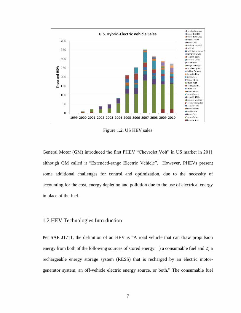
accepted by the customers. HEV sales in US is growing steadily (Figure 1.2) [4]. From
1999, the first HEV sold in US, to 2010, almost 2 millions HEV on US roads. Although
there are still many unsolved challenges on the technologies and markets, the HEV,
particularly PHEV seems to be the most promising short-term solutions to reduce the fuel
consumption and emissions.
PHEVs with oversized batteries that can also be recharged using electric power from the
grid, have recently become a hot topic in the automotive industrial because of the
undoubted advantages in terms of emissions and fuel consumption deriving from the
possibility to be driven for a relatively extended driving range using only electricity.
7
Figure 1.2. US HEV sales
General Motor (GM) introduced the first PHEV “Chevrolet Volt” in US market in 2011
although GM called it “Extended-range Electric Vehicle”. However, PHEVs present
some additional challenges for control and optimization, due to the necessity of
accounting for the cost, energy depletion and pollution due to the use of electrical energy
in place of the fuel.
1.2 HEV Technologies Introduction
Per SAE J1711, the definition of an HEV is “A road vehicle that can draw propulsion
energy from both of the following sources of stored energy: 1) a consumable fuel and 2) a
rechargeable energy storage system (RESS) that is recharged by an electric motor-
generator system, an off-vehicle electric energy source, or both.” The consumable fuel

8
that is covered in this study is limited to the gasoline. RESS that is covered in this study
is the battery.
Comparing with the conventional vehicles, HEVs or PHEVs not only reduce the green-
house gas emissions, but also have less fuel cost (Table 1.3) [5]. HEVs were categorized
into serial and parallel HEV on the conventional concept. As the HEV development
getting more and more attentions, various designs and technologies emerge and were
applied to the production vehicles. The categorization and evaluation of HEV have been
an important project to be studied to direct the HEV development and research [6-9].
Considering the HEV powertrain functions, architectures, and vehicle packages, the
design of the HEV powertrain has a high level of degree of freedom. These designs can
be categorized by their degrees of hybridization or their powertrain configurations.
Based on the degree of hybridization, the HEVs can be categorized full hybrid and mild
hybrid. The hybridization always is determined into the ratio of the power of the
propulsion motor to that of the engine. A full hybrid, sometimes also called a strong
hybrid, is a vehicle that can run on just the engine, just the batteries, or a combination of
both. The full HEV can be operated at different distinct regimes: electric mode, cruise
mode, overdrive mode, battery charge mode, power boost mode, and negative split mode.
Mild hybrids are essentially conventional vehicles with some degree of hybrid hardware,
but with limited hybrid feature utilization. Typically they are a parallel system with start-
stop only or possibly in combination with modest levels of engine assist or regenerative
braking features. Unlike full hybrids, Mild hybrids generally cannot provide ICE-OFF

9
Table 1.3. Comparison of Emissions and Fuel Cost of X-vehicles
Emissions and Fuel Cost for a 100-Mile Trip
Vehicle Greenhouse Gas Emissions Total Fuel Cost
(compact sedans) (pounds of CO2 equivalent) (U.S. Dollars)
Conventional 87 lb CO2 $13.36
Hybrid Electric 57 lb CO2 $8.78
Plug-in Hybrid Electric 62 lb CO2 $7.10
All-Electric 54 lb CO2 $3.74
all-electric propulsion. A plug-in hybrid electric vehicle is one of the full hybrids, able to
run in electric-only mode, with larger batteries and the ability to recharge from the
electric power grid. And can be parallel or series hybrid designs. They are also called
gas-optional, or griddable hybrids. Their main benefit is that they can be gasoline-
independent for daily commuting, but also have the extended range of a hybrid for long
trips. Basically, the higher the hybridization the vehicle is, the more improvement of the
fuel economy and emissions are. The hybridization of Honda Civic is 15.9% which is the
mild hybrid. The hybridization of Toyota Prius is 62.3% which is the full hybrid.
Based on the powertrain system design, several kinds of hybrid electric vehicles have
been conceived, usually distinguished by their architecture, which is related to the path
that the power flow follows from the energy sources to the wheels. They are (see Figure
1.3): series hybrid, parallel hybrid, and power-split hybrid.
The series configuration is the simplest architecture in the hybrid electric vehicles. The
engine directly drives the generator which transforms the mechanical power from engine

10
into the electric power and supplies the power to the power storage device through the
inverter, or to the propulsion motor directly. The serial HEV is driven by the propulsion
motor. The engine, as the auxiliary driving unit, extends the driving range of the vehicle.
The motor power is supplied by either a power-storage device, or a generator, or the
combination of both with a split ratio determined by the power management controller.
Since the engine operation is independent of the vehicle speed and road condition, it is
controlled to operate near its optimal condition most of the time. In addition, because the
mechanical power transition path is eliminated, the energy loss due to the torque
converter and the transmission is avoided. However, because of more processes to
convert and transform, the energy from the engine to the wheels results in the lower
efficiency. In addition, all of the serial elements, such as the engine, generator, and motor,
need the extra stand-by powers to meet the vehicle dynamics requirements.
In a parallel configuration, the single electric motor and the engine are installed such that
they can power the vehicle either individually or together. The engine mainly supplies the
power to drive the vehicle. Meanwhile the motor works as the auxiliary power unit. The
role of the motor is to assist the engine to operate efficiently and to capture regenerative
braking energy. Comparing with the series HEV, the engine is larger and more powerful,
while the motor is smaller and less powerful. The main advantage of the parallel hybrid
vehicle is the relatively high efficiency. The engine power is directly transferred to the
wheels and therefore no power conversion is needed. The main disadvantage of the
parallel hybrid vehicle is the engine speed is directly coupled to the vehicle speed and
road condition and therefore the engine can not be operated in the most economic point
continuously.

11
a) Series Hybrid
b) Parallel hybrid
c) Power-split hybrid
Figure 1.3. HEV configurations
B: Battery
E: Engine
G: Generator
I: Inverter
M: Motor
T: Transmission
W: Wheel
-: Electric Link
=: Mechanical Link

12
The power-split configuration (also called series-parallel HEV) combines the parallel and
series powertrains. The power from the engine is split. One part of the power is
transferred to the wheels through a mechanical path. The other part flows to the wheels
via the electric path, which consists of the generator and the electric motor. A power split
device (PSD), which is a planetary gear set, connects the engine, motor, and generator to
work as a continuously variable transmission (CVT) and provides the advantage of
adjusting the engine in the economic operation range. The generator is used to control the
engine speed, the motor controls the engine torque. The generator is also used to convert
excessive engine power to electric power that can be stored in the battery. The motor is
operated for the power supply and for the recovery of energy during braking. Since only a
small part of the engine power flows through the electric path, most of the power will be
directly transferred to the wheels via a mechanical connection. This mechanical
connection has a high efficiency. Therefore, the efficiency of the power-split
configuration is high compared to the series.
1.3 Power Split Device Architecture Introduction
The earliest development of the power split mechanisms can be tracked back to 1969 [10].
But this power-split concept was not applied to passenger vehicles until the late 1990s.
The first production power-split passenger vehicle is the Toyota Hybrid System (THS)
[11] (Figure 1.4) which is known as the single mode PSD system. THS is vastly applied
on the Toyota HEVs, such as Prius, and becomes the front-runner on the market. The
advantage of the THS PSD is its relative simplicity and its increased performance over
competing hybrid designs. However, the performance and fuel economy at high speeds
and on steep grades is not outstanding due to the undersized engine and low efficiency at

13
high speed. This is common to many vehicle types, because actual driving conditions are
different than the idealized conditions in the laboratory testing, such as faster
accelerations and higher top speeds.
Another major design for power-split HEV on the market is the Allison Hybrid System
(AHSII) (Figure 1.5) [12] which is invented by GM as a dual-mode PSD system in 2003.
The main difference between single mode and dual mode PSD is the addition of clutches
and/or brakes to create different transmission configurations. This increases the number
of possible power flow paths through the transmission. The clutches are engaged and
disengaged based on the system information such as the engine/motor efficiency maps,
battery SOC, road load and driver demand to determine the operation mode. The dual-
mode PSD system provides more efficient performance over a wider range of vehicle
loads than that achieved by the single-mode design. However, the additional mechanical
components will certainly increase both capital and maintenance costs.
Many other power split designs are developed by different companies. Bosch developed a
power split transmission with circulating power for the hybrid electric vehicles [13] in
2004. GETRAG tested their democar with axle-split and torque-split hybrid
transmissions to reduce the fuel consumption 24% and 35% respectively [14]. Ford
Motor Company installed the power split transmission in Ford Escape Hybrid and
brought to the market in 2004. Renault also developed a dual mode power split
transmission [15].

14
Figure 1.4. Single mode PSD system (Source: adapted from [13])
Figure 1.5. Dual mode PSD system (Source: adapted from [13])
1.4 Literature Review
1.4.1 Modeling power-split system
The proper modeling and simulation tools can shorten the vehicle development timing,
reduce the development cost, validate the HEV control strategy, evaluate the vehicle
performance, etc. in the early design and analysis stage. A considerable amount of work has

15
been done in the power split system modeling and simulation. A dynamic model (Zhang et
al.) was created to evaluate an electric variable transmission (EVT) developed by Allison
Transmission Division of General Motors [16]. The model is based on Kane's equations,
and the concept of generalized velocity is used. The EVT performance was simulated by
using the model. A mathematical model [17] of a vehicle with a power-split device based on
the steady-state performance was presented by the researchers from Michigan Technological
University (Rizoulis et al.). A math-based universal model [18] that presents different
designs of power-split powertrains was created (Liu). This universal model presents the
powertrain dynamics regardless of the various connections of engine-to-gear, motor-to-
gear, and clutch-to-gear. A dynamic model (Zanasi et al.) of a planetary gear with
internal elasticity [19] was presented. The model of the whole vehicle is given using the
Power-Oriented Graphs approach. A dynamic model [20] of a multi-regime hybrid
vehicle powertrain architecture (Wishart et al.) was presented to focus on the formulae
governing the operation of the planetary gear systems in the powertrain and on the
performance of a more complex heavy-duty vehicle with varying loading conditions.
1.4.2 Energy management optimization of power-split HEVs
The research of the energy management optimizations has been done on the different
configuration of HEVs design. The global optimization and the local optimization of the
HEV energy management are two major research directions. The typical represents of the
global optimization are the Dynamic Programming (DP) [21]-[25] and Pontryagin’s
Minimum Principle (PMP) [26]-[29]. The typical example of the local optimization is
Equivalent Fuel Consumption Minimization (ECM) [30]-[34]. Many papers about the power

16
split HEVs energy management optimization have been published. Banvait et al. [35]
studied the energy control strategy of the plug-in hybrid electric vehicle with PSD using
particle swarm optimization. Liu [36], [37] presented a stochastic dynamic programming
method and the equivalent consumption minimization strategy to optimize the single
mode power split HEV. Both approaches determine the engine power based on the
overall vehicle efficiency and apply the electrical machines to optimize the engine
operation. The performance of these two algorithms is assessed by comparing against the
simulation results. Bole [23] also presented a dynamic programming method and the
equivalent consumption minimization strategy to optimize the dual mode power split
HEV. The optimization results of dynamic programming and equivalent consumption
minimization compared with the developed rule-based control strategy simulation results.
Moura [24] presented a dynamic programming method with consideration of trade-off of
the fuel and electricity of usage and the fuel-to-electricity pricing to optimize the single
mode PHEV energy management.
1.4.3 Control strategy of power-split HEVs
The supervisory control system represents the vehicle level controller that coordinates the
sub-systems to satisfy certain performance targets. Control Strategy is the algorithm to make
the controller to achieve the vehicle energy management and control the power systems. It is
the vehicle “brain” and is the ultimate factor to determine the success or failure of a HEV
development. So far, most of the research on the HEV control strategy is still on the
computer simulation stage, particularly for the instantaneous optimal control strategy and the
global optimal control strategy. It is difficult for them to be applied on the commercial

17
vehicles because of the heavy burden computation and very expensive high performance
CPU. Although some vehicle OEMs, such as Toyota, GMC, Honda, are selling the HEVs
with developed control strategies, those control strategies are companies’ core technical
secrets and can not be published.
Most of the early HEV control strategies are the speed – based control algorithms [38], [39]
because it is simple and easy to be understood. The vehicle speed is the critical parameter in
the control strategy. When the vehicle speed is lower then the threshold setup, the engine will
be turned off. When the vehicle speed is higher then the threshold setup, the engine will be
started. However, the disadvantage of the speed-based control strategy is that when the
vehicle is driven at the high speed cruise, the engine may operate at the low efficiency zone.
The current control strategy is the torque-based control algorithm. The torque-based control
strategy reasonably distributes the torque required by vehicle wheel between the engine,
motor and generator to minimize the vehicle fuel consumption and emissions. The objective
of the control strategy is to improve the vehicle fuel economy and reduce the emissions, so
the rules to develop the control strategy are as follows:
Control the engine to be operated at high efficiency zone.
Keep the motor to be operated at high efficiency zone.
Maintain the battery SOC to be within the specific range.
The current presented torque-base HEV control strategies include:
Rule-based control strategy by adjusting the engine operation zone.
Instantaneous optimal control strategy by real time calculating to determine the
engine and motor/generator optimal operation points.

18
Global optimal control strategy by applying the optimal control theory.
Fuzzy logic or neural network intelligent control system.
Despite the early efforts, to my knowledge, the effects of the power-split planetary gear
ratios to the vehicle fuel consumptions and operation costs do not yet exist in the
literature. It is important and significant to optimize the PSD gear ratio to minimize the
vehicle fuel consumptions and operation costs.
1.5 Contribution
This thesis focuses on the process of the single mode power-split PHEV (Figure 1.6)
modeling, energy management optimization, ruled-based control strategy development,
Figure 1.6. PHEV configuration and energy flow. (E– engine, G – generator, M – motor,
W – wheel, I – Inverter, B - Battery).

19
and investigation of the effects of PSD gear ratios to the PHEV fuel consumptions and
operation costs. A dynamic power-split PHEV simulation model is derived. By using this
model, an optimal solution for the power-split PHEV with its benchmark performance is
provided through the dynamic programming. The rule-based control strategy is then
developed and the control strategy parameters are optimized by using the genetic
algorithm. The effects of PSD gear ratios to the PHEV fuel consumptions and operation
costs at the different driving cycles are finally discussed in this thesis. The main
contributions of the thesis include the following:
A backward-looking dynamic model of the power-split PHEV powertrain systems
is created. The engine, power-split device, motor/generator, battery, and vehicle
dynamics are integrated to perform a simulation. This simulation tool can be used
to analyze the interaction between sub-systems and evaluate vehicle performance
using measures such as fuel economy and operation costs.
An optimal control design procedure based on dynamic programming (DP) is
adopted in the power-split HEV fuel efficiency optimization study. DP is
employed to find the optimal operation of the power-split system and achieve the
benchmarks. The results are then applied to develop the real time control strategy
designs.
A rule-based control strategy based on the DP optimal results is developed. The
comparisons between the rule-based control strategy and optimal benchmarks are
discussed at different driving cycles. The developed rule-based control strategy is
then applied to investigate the PSD gear ratios to PHEV fuel consumptions and
operation costs at the different driving cycles.

20
The rule-based control strategy parameters of the power-split PHEV are
optimized by using non-dominated sorting genetic algorithm (NSGA-II). NSGA-
II is employed to find the optimal control strategy parameters to minimize the
vehicle fuel consumptions and operation costs. The results provide the engineers
the fast and economic vehicle control strategy tunings.
An innovative six-step approach to design the power split PHEV planetary gear
ratio to minimize the fuel consumption and operation cost is presented.
1.6 Outline of the Thesis
The organization of this thesis is as follows. After the introduction in Chapter 1, the
development of an integrated model for power-split plug-in hybrid electric vehicles is
presented in Chapter 2. The optimal control by using dynamic programming is presented
in Chapter 3. Chapter 4 presents the development of the rule-based control strategy for
PHEV. Chapter 5 presents the optimization of rule-based control strategy parameters by
using genetic algorithm NSGA-II. An innovative design approach to optimize the PSD
gear ratio to minimize the vehicle fuel consumption and operation cost is developed in
Chapter 6. Finally, a summary of this thesis and suggested future work are presented in
Chapter 7.

21
CHAPTER 2
MODELING PHEV SYSTEMS
2.1 Introduction
Based on the level of details of the each modeled component, the vehicle model may be
steady-state, quasi-steady, or dynamic. For example, the ADVISOR [40], [41] model can
be categorized as a steady-state model, the PSAT [42] model as quasi-steady one, and
PSIM [43] and Virtual Test Bed (VTB) [44] models as dynamic. On the other hand,
based on the direction of calculation, vehicle models can be classified as forward-looking
models or backward facing models [40] (See Figure 2.1 and Figure 2.2). In a forward-
looking model, vehicle speed is controlled to follow a driving cycle during the analysis of
fuel economy, thus facilitating the controller development.
Figure 2.1. Flow diagram of the backward-looking model
Figure 2.2. Flow diagram of the forward-looking model

22
When using backward-looking models, the control logic does not have to be considered
complicated system constraints because the models calculate the exact torque or speed
that a system requires and allow the controller to have only feasible control options. In
contrast, in forward-looking models, the controller considers constraints and component
losses and instantaneously makes decisions for the entire system. Therefore, the
controller needs to collect the information required from the components and produces a
control signal according to time-forward strategies. In this chapter, a backward-looking
simulation model is developed for the power-split plug-in hybrid vehicles. The simulation
model is implemented in the Matlab environment.
2.2 Engine Model
Figure 2.3 is the diagram of the inputs and outputs of the engine model. The inputs
include the engine output torque and speed, and the outputs required are engine operation
efficiency, fuel consumption rate, emissions, operation fuel cost. The inputs and outputs
of the engine model are just considered during analysis the PHEV energy management.
The theoretical engine model is not superior to the experimental engine model because of
the accuracy caused by the many assumptions and the expensive computer operation cost.
So the experimental engine model always used to simulate the HEV powertrain system.
Figure 2.3. Inputs and outputs of the engine model

23
In order to support the computation over long driving cycles, a look-up table is used that
provides torque as a function of engine speed and mass of fuel injected per cycle. The
engine dynamics are ignored. The assumption is made that the working condition is at
constant average level. The fuel consumption is evaluated by (2.1):
t t
t lve
eeee
t
ffH
TdtTfdtmm
0 00
),(
(2.1)
The fuel consumption map, in g, of the engine as function of the engine speed and engine
torque is shown in Figure 2.4.
2.3 Motor/Generator Model
Figure 2.5 is the diagram of the inputs and outputs of the motor/generator model. The
input is the motor/generator output speed. The model outputs include the motor/generator
output torque, power, efficiency and electricity operation cost.
0200
400600
800
0
50
1000
1
2
3
4
5
x 10-3
Speed (rad/s)Torque (Nm)
Fu
el C
0n
sum
pti
on
(g
)
Figure 2.4. Engine fuel consumption map

24
Figure 2.5. Inputs and outputs of the Motor/Generator model
Same as the engine model, the inputs and outputs of the motor/generator model are just
considered during analysis the PHEV energy management. The look-up tables provide
efficiency of the motor/generator as a function of the torque and speed. The
motor/generator is the function of torque and speed, η=f(T, ω). When motor/generator
consumes the energy, which means the power flows from battery to the motor/generator,
the consumed power is represented by (2.2).
MG
MGMGMG
TP
(2.2)
When the motor/generator generates electrical energy, which means the power flows
from motor/generator to the battery pack, the generated power is represented by:
MGMGMGMG TP (2.3)
Equations (2.2) and (2.3) will be used for the battery State-of-Charge (SOC) calculation.
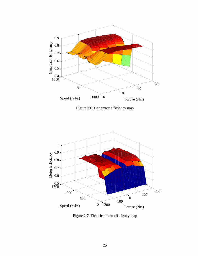
Figure 2.6 and Figure 2.7 are the efficiency maps for the Toyota Prius motor and
generator which are at 15 kW and 35 kW respectively.
25
0
20
40
60
-1000
0
10000.4
0.5
0.6
0.7
0.8
0.9
Torque (Nm)Speed (rad/s)
Gen
eraa
tor
Eff
icie
ncy
Figure 2.6. Generator efficiency map
-200-100
0100
200
0
500
1000
15000.5
0.6
0.7
0.8
0.9
1
Torque (Nm)Speed (rad/s)
Mo
tor
Eff
icie
ncy
Figure 2.7. Electric motor efficiency map

26
2.4 Battery Model
Figure 2.8 is the relationship of the input and output of the battery model. The inputs
include the battery capacity Q, internal resistance Rint , open circuit voltage VOC, and
battery power output Pbatt. The output is the battery SOC. The battery model is
represented by an equivalent circuit with an internal resistance, as shown in Figure 2.9.
The battery Rint is the function of the SOC and the current direction Ibatt (Figure 2.10):
),(int battISOCfR
(2.4)
The battery SOC is the function of the VOC (Figure 2.11):
)( OCVfSOC (2.5)
Both functions are obtained through the curve fitting based on the battery test results.
Figure 2.8. Inputs and outputs of the battery model
Figure 2.9. Battery electrical equivalent circuit
ernalRint BattI
BattPOCV

27
Figure 2.10 Battery internal resistance map with SOC
Figure 2.11. Battery open circuit voltage map with SOC
The battery pack dynamics are associated with SOC, and SOC depends on the equivalent
battery capacity Q and the current flowing through the battery IBatt:
QI
COS Batt (2.6)
The battery output power is a function of VOC, IBatt, and Rint:
int
2 RIIVP BattBattOCbatt (2.7)

28
This expression may be written in terms of SOC and solved to obtain the equation for
SOC:
int
int
2
2
4
QR
RPVVCOS
BattOCOC
(2.8)
The power required from the battery will be:
k
C
k
MGMGMGBatt TP (2.9)
Where, k=1 when power flows to the battery and k=-1 when power flows away from the
battery.
2.5 PSD Model
The planetary gear set is the core of the power split transmission as shown in Figure 2.12.
The planetary gear set consists of a ring gear, a sun gear, a carrier, and pinion gears
where the engine is connected to the carrier, the generator to the sun gear, and the motor
to the ring gear and final driveline. The basic gear ratio of the planetary gear set follows:
kR
R
s
r
cr
cs
(2.10)
Figure 2.12. PHEV planetary gear set

29
The relationships between the torques are:
cs Tk
kT
1 (2.11)
k
TTT c
rf
1
(2.12)
Figure 2.13 shows the free body diagram of planetary gear set. The relationships between
the torques are:
ssss
rsccc
rrrr
TFZI
ZZFTI
TFZI
)( (2.13)
2.6 Powertrain Dynamic Model
Figure 2.14 shows the free body diagram of the powertrain. The torques determine the
rotational speeds in the transmission. The powertrain dynamic equations are following:
dfmrfrrm
sggg
ceee
TZTTZII
TTI
TTI
)()(
(2.14)
Combining equations (2.10)–(2.14), and only considering the vehicle dynamics along the
longitidinal direction which is the dominating factor for the fuel economic, the
powertrain dyamic model can be derived:
00
00
020
00
g
f
dm
e
s
r
e
srsr
ssg
rrm
srce
T
Z
TT
T
FRRRR
RII
RII
RRII
(2.15)
Where:
tiretd RFT (2.16)

30
Figure 2.13. Free body diagram of planetary gear set
Figure 2.14. Free body diagram of powertrain

31
2.7 Vehicle Model
Figure 2.15. Vehicle free body diagram
The propulsion system produces mechanical energy that is stored in the vehicle. The
amount of mechanical energy consumed while driving the vehicle depends on the
following effects:
The aerodynamic friction losses
The uphill driving losses
The rolling friction losses
The vehicle model is derived from the basic equation of solid-body motions (Figure 2.15):
rgadt FFFFdt
dvm (2.17)
25.0 VACF FDad (2.18)

32
sinmgF g (2.19)
cosmgfF rr (2.20)
2.8 Summary
The backward-looking model of PHEV was created in this chapter under Matlab
environment. It provided the necessary platform to simulate the PHEV fuel consumption
and study the control strategy. The main study in this chapter focused on following:
1. The look-up table based PHEV engine, motor/generator, and battery models were
created. Those models represent the static state of the systems. However, the
simulations will focus on the PHEV energy consumptions, so the model accuracy
is enough.
2. The dynamic PSD and powertrain system models were created based on the
system loads balances.
3. The vehicle model was created by applying the vehicle longitudinal dynamics.

33
CHAPTER 3
OPTIMAL CONTROL OF PHEV
3.1 Introduction
The optimal energy management of HEV is a global optimization problem whose
objective is to determine the power split between the engine and the motor to minimize
the vehicle fuel consumption and operation cost. Comparing with other optimal
approaches, such as Pontryagin’s Minimum Principle (PMP) [45], [46], the Equivalent
Consumption Minimization Strategy (ECMS) [35], [46], the DP approach guarantees the
global optimal results and the results are unbeatable under the given driving cycles. In
this study, the DP approach was used to optimize the PHEV control strategy to minimize
the fuel consumption and operation cost.
3.2 Mathematic Model of Optimal Control
Figure 1.4 shows the PHEV configuration in this study. From the Figure 2.12 and
equation (2.14) and (2.15), the relationship of the torque on the wheels with the engine
torque and motor/generator torque can be derived:
f
d
fgr
s
fer
srg
g
se
e
sr
m
gr
s
er
srrr
fgr
sm
fer
srm
T
iIZ
Z
iIZ
ZZT
I
ZT
I
ZZ
TIZ
Z
IZ
ZZZ
iIZ
ZI
iIZ
ZZI
22
2222
)()(
)()(
(3.1)
The same routine to derive the relation of the engine speed and the engine torque:

34
f
d
m
rg
g
sm
m
fr
e
gsr
s
msr
fr
esr
gsr
se
msr
fre
T
I
ZT
I
ZT
I
ZZT
IZZ
Z
IZZ
ZZ
ZZIZZ
ZI
IZZ
ZZI
)()(
)()()(
22
22
(3.2)
The relation of the motor speed and vehicle speed is written:
ftire
mZR
v
(3.3)
The constrains of the components are as following:
max,min, eee TTT (3.4)
max,min, eee (3.5)
max,min, ggg TTT (3.6)
max,min, ggg (3.7)
max,min, mmm (3.8)
max,min, mmm TTT (3.9)
For a given drive cycle, the vehicle speed at the given time is known. Considering
equations (3.1) - (3.3), there are only two independent variables: motor torque Tm and
generator torque Tg. The engine torque Te can be derived from the motor torque Tm and
generator torque Tg. The engine speed can be derived from the engine torque Te.
The state variable of the PHEV is defined as following:
)]([)( tSOCtx (3.10)

35
SOC(t) is the battery state of charge at the time t. it meets following constrain:
maxmin SOCSOCSOC (3.11)
The control variables are determined:
)](),([)( tTtTtu gm (3.12)
And they meet the constrains of (3.4) to (3.9).
Given the driving cycle, the PHEV optimal control can be expressed: it is desired to
determine a control law to minimize the performance measurement, from the initial state
)]0([)0( SOCx to the end of state )]([)( ff tSOCtx at the driving cycle time
ft . The optimal function of the PHEV is:
ft
dttutxLJ0
))(),(( (3.13)
For the PHEV, the fuel consumption function includes the fuel consumption and
electricity consumption during the vehicle operation. The fuel consumption function can
be described:
)()()(),(( telectrictfueltutxL electric (3.14)
3.3 Dynamic Programming
Dynamic Programming (DP) [47] which was developed by Bellman is a powerful tool to
transform the complex decision-making problem to a series of sub-problems by the

36
global optimization. For a given driving cycle, the optimal operation strategy to minimize
fuel consumption, or combined cost of fuel/electricity consumption can be obtained.
Due to the nonlinear characteristics of the hybrid powertrain, it is not possible to solve
DP analytically. Instead, DP has to be solved numerically by some approximations.
Equation (3.13) is a continuously operating system which can be approximated by a
discrete system by considering N equally spaced time increments in the interval
ftt 0 . Due to the fact that the system level dynamics are the main concern to
evaluate fuel economy over a long driving cycle, dynamics that are much faster than 1 Hz
could be ignored [48]. The sample time for the main-loop control problem is selected to
be 1 second. The discrete-time model of PHEV can be described as:
kukxfkx ,1 (3.15)
The state variable is SOC: )(),()(1 kTkTfkSOCkSOC gm . (3.16)
The cost function of the PHEV powertrain can be expressed as:
1
0
1
0
),(
N
kGrid
Battelectricfuelfuel
N
k
PP
kukxLJ
(3.17)
Assume that the fuel price ratio is β=0.65, which is consistent with the energy price in the
year 2010: $2.77 USD per gallon of gasoline and $0.1145 USD per kWh of electricity
[49].

37
The optimization goal is to find the control variable, u(k), to minimize the cost function.
The optimization problem is subject to a set of inequality constraints arising from the
component speed, torque and SOC characteristics. The constraints for state X:
maxmin SOCSOCSOC
edischbatteryech PPP argarg
max,min, MMM
max,min, GGG
max,min, GGG TTT
The constraints for control U:
max,min, MMM TTT
max,min, eee TTT
max,min, eee
In addition, one equality constraint for optimization problem is imposed the drivability,
GMedem PPPP (3.18)
Based on Bellman’s principle, the DP algorithm is presented as follows:
))]1(),1(([min)1(
*
1
NuNxLJNu
N (3.19)
Step k, for 0≤k<N-1:
))]1(())(),(([min))(( *
1)1(
*
kxJkukxLkxJ kNu
k (3.20)
and:
0))((* NxJk (3.21)

38
The dynamic programming process consists of two parts. The first part can be
characterized as a backward procedure, because it travels through the states starting from
the destination and finishing at the origin. The recursive equation is solved backwards
from step N-1 to 0 in order to find the optimal control policy. Each of the minimizations
is performed subject to the constraints above and the driving cycle. The optimal
performance measurement ))((* kxJk and optimal control u(k) can be obtained at every
step under the related state. Similarly, the second part is a forward procedure which
traverses the states starting from the origin and moving towards the destination to
determine the optimal control policy and optimal trajectory.
A standard way to solve equation (3.20) numerically is to use quantization and
interpolation [50]-[52]. For continuous state space and control space, the state and control
values are first discretized into finite grids. At each step of the optimization
Figure 3.1. Numerical dynamic programming algorithm

39
search, the function is evaluated only at the grid points of the state variables. If the next
state does not fall exactly on a quantized value, then the values of in equation (3.20) as
well as in equation (3.19) are determined through linear interpolation.
3.4 Reduction of Dynamic Programming Grid Size
In order to reduce the computation burden of dynamic programming, the “limit
trajectories” [53], [54] approach is used to reduce the grid size. If the initial state x(0) is
defined, it is possible to bound a region in the state space by means of the limit
trajectories. Those state space trajectories obtained apply the extreme controls to the
system equations. The only states to be explored are confined in the region defined by
these trajectories and the constraints. Because the state variable is SOC, the SOC limit
trajectories are determined as follows:
When the wheel torque wheelT > 0, the maximum electricity consumption will be based on
the maximum motor torque )(_ kT him . )(_ kT him is the smallest of the following three:
1) i
kTwheel )(
;
2) The maximum motor torque provided by the motor;
3) The maximum output motor torque under the limitation of the battery discharge
capacity;
When the wheel torque wheelT < 0, the maximum electricity generated by the motor will be
based on the maximum motor torque )(_ kT lom . )(_ kT lom is the largest of the following
three:

40
1) i
kTwheel )(
;
2) The maximum motor torque provided by the motor;
3) The maximum output motor torque under the limitation of the battery charge
capacity;
Figure 3.2 shows the SOC limit trajectories. The state SOC will be explored in the limit
trajectory boundaries. In this way, the calculation burden is greatly reduced.
3.5 Simulation Results
The DP optimal control is applied to PHEV in appendix I to calculate the vehicle fuel
consumption. Figure 3.3 shows the SOC limit trajectories of UDDS driving cycle.
Because the PHEV battery is charged before the operation, and considering the battery
operation range, the highest SOC value is set to 0.9 and the lowest is set to 0.32. The grid
size of the state variables and the control signals will directly influence the simulation
accuracy and computational cost. Small grid sizes lead to longer computation time but more
accurate optimization results and larger grid sizes save computational cost but may obtain
Figure 3.2. The limit trajectory boundaries

41
Table 3.1. The Selected Grid Points in DDP
States
SOC 0.32:0.005:0.9
Controls Inputs
Motor Torque [Nm] -300:15:300
Generator Torque [Nm] -55:5:55
inaccurate results. Also, the state and input grids need to be coherent. A state grid may not be
reached by the control. The selected grid points are shown in Table 3.1.
Figure 3.4-3.6 are the simulation results of SOC, motor torque, engine torque and powers
in two (2) driving cycles. The fuel consumption of 2 UDDS driving cycles is 273.93g
(1.55L/100km) which is the best fuel economy that the PHEV can achieve. Any other
control strategies can’t compete this result.
3.6 Summary
The optimal control model of PHEV was created under the condition of given driving
cycles to optimize the vehicle fuel consumption and operation cost in this chapter. The
optimal control strategy was obtained by the DP approach. The optimal control strategy
not only can evaluate the real time control strategy, but also direct the real time control
strategy optimization. The purpose of this study is to determine the global optimal fuel
consumption and operation cost as the benchmark of the real-time PHEV control
strategy. The main study in this chapter focused on following:
The optimal control model of PHEV was created. The state variable of the
optimal control model is SOC, the control variables are the motor and generator

42
torques. In order to reduce the computation burden, the “limit trajectories”
approach is used to reduce the grid size.
The step was set to 1 second which was determined based on the given driving
cycles. The assumption was made that the vehicle fuel consumption is constant
within each steps, therefore changing the continuous optimal control to a series of
sub-problems.
The optimal results are the best PHEV fuel consumptions by using DP approach.
Figure 3.3. The limit trajectory boundaries for UDDS Driving cycle

43
0.3
0.4
0.5
0.6
0.7
0.8
0.9
1
0 400 800 1200 1600 2000 2400 2800
Time (s)
SO
C
Figure 3.4. DP simulation results – SOC
-250
-200
-150
-100
-50
0
50
100
150
200
250
300
0 400 800 1200 1600 2000 2400 2800
Time (s)
Mo
tor
To
rqu
e (N
m)
Figure 3.5 DP simulation results – Motor Torque

44
0
10
20
30
40
50
60
70
80
90
100
0 400 800 1200 1600 2000 2400 2800
Time (s)
En
gin
e to
rqu
e (N
m)
Figure 3.6. DP simulation results – Engine Torque
-40000
-30000
-20000
-10000
0
10000
20000
30000
40000
0 400 800 1200 1600 2000 2400 2800
Time (s)
Po
wer
(W
)
Engine Power
Motor Power
Required Power
Figure 3.7. DP simulation results – Power

45
CHAPTER 4
PHEV RULE-BASED CONTROL STRATEGY
4.1 Introduction
Due to the multiple-power-source nature and the complex configuration and operation
modes, the PHEV energy management is implemented by effectively controlling of the
multiple power sources. The algorithm of the vehicle energy management and power
systems control is called the control strategy. The PHEV control strategy and the vehicle
controller are the vehicle nerve center and more complicated than that of an engine-only
vehicle. The main function of the control strategy is the power management, i.e., the
design of the high-level control algorithm that determines the proper power split between
the motor and the engine to minimize fuel consumption and emissions, while satisfying
constraints such as drivability, charge sustaining and component reliability.
The HEV control strategy studies mainly focus on the three areas: rule-based control
strategy [55], [56], real time local optimization [57], [58], and fuzzy-logic/neural network
intelligent control strategy [59], [60]. Because of the expensive computer operation cost
of the real time local optimization, it currently cannot be applied on the commercial
HEV. The popular control strategy used in the commercial vehicles is the rule-based
control strategy [61], [62]. The fuzzy-logic/neural network intelligent control strategy has
been applied in different engineering fields. The fuzzy logic control strategy is also used
on the HEV.

46
In this chapter, a rule-based control strategy for PHEV will be developed based on the
PHEV optimal control strategy created in Chapter III.
4.2 PHEV Torque Balance Control
From equation 2.16, the torque on the driveline is tiretd RFT . The energy management
control strategy should meet the requirement of the torque demanded from vehicle
wheels. The energy management control strategy will determine the power split ratio of
the engine to the motor. When the torque on the driveline dT is positive, then:
mdred TTT _ (4.1)
gdree TTT _ (4.2)
Where gme TTT ,, are the torques of the engine, the motor and the generator. dreT _ is the
torque which is transferred from the engine to the driveline. The torque of the generator is
always negative to adjust the engine torque based on the engine efficiency map. When
the torque on the driveline dT is negative, then:
brakemd TTT (4.3)
Where brakem TT , are the torques of the motor and the hydraulic brake.
The goal of the control strategy is to choose an operating point that minimizes the
engine’s fuel consumption and emissions. The engine will be operated in the economic
area which follows opteT _ curve. When the engine torque falls below the limit offeT _ , the
engine will be shut off. At the same time, the negative generator torque adjusts the engine
always operate upper the opteT min__ .

47
In order to determine the engine economic area, the engine directly driving efficiency and
the motor driving efficiency would be compared, therefore determining opteT min__ and
offeT _ .The engine directly driving efficiency:
de1 (4.3)
The motor driving efficiency with the energy from the engine:
dminvgopte _2 (4.4)
If 21 , then the engine operation point is not in the economic area. The engine should
be shut off and the engine torque would be offeT _ . If just considering the battery charging,
the minimum optimal engine torque opteT min__ would be determined. However, the torques
would be setup as the final control strategy parameters by optimization and calibration on
the vehicle. The control strategy parameters optimization will be discussed in next
chapter.
4.3 PHEV Operation Modes
Most of the rule-based control strategies are based on “IF-THEN” type of the control
rules and perform the load balancing between the power sources. The typical PHEV
control strategy is PSAT control strategy which is based on charge-depleting (CD) mode
and charge-sustaining (CS) mode. The global energy management optimization of PHEV
and PHEV control strategy testing show that the blended control strategy has better
energy efficiency compared with the electric-only control strategy. The PHEV uses 6
operation modes to achieve the most efficient operation in response to the driving
conditions based on the blended control strategy in this study.
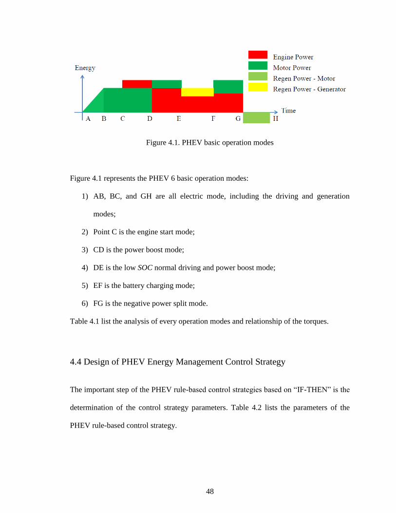
48
Figure 4.1. PHEV basic operation modes
Figure 4.1 represents the PHEV 6 basic operation modes:
1) AB, BC, and GH are all electric mode, including the driving and generation
modes;
2) Point C is the engine start mode;
3) CD is the power boost mode;
4) DE is the low SOC normal driving and power boost mode;
5) EF is the battery charging mode;
6) FG is the negative power split mode.
Table 4.1 list the analysis of every operation modes and relationship of the torques.
4.4 Design of PHEV Energy Management Control Strategy
The important step of the PHEV rule-based control strategies based on “IF-THEN” is the
determination of the control strategy parameters. Table 4.2 lists the parameters of the
PHEV rule-based control strategy.
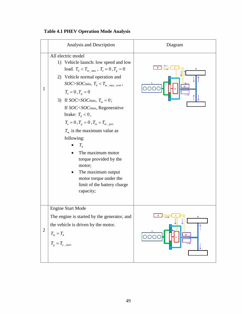
49
Table 4.1 PHEV Operation Mode Analysis
Analysis and Description Diagram
1
All electric model
1) Vehicle launch: low speed and low
load. max_md TT , 0eT , 0gT
2) Vehicle normal operation and
SOC>SOCmin, contmd TT max__ ,
0eT , 0gT
3) If SOC>SOCmax, 0mT ;
If SOC<SOCmax, Regenerative
brake:
0dT ,
0eT , 0gT , genmm TT _
mT is the maximum value as
following:
dT
The maximum motor
torque provided by the
motor;
The maximum output
motor torque under the
limit of the battery charge
capacity;
2
Engine Start Mode
The engine is started by the generator, and
the vehicle is driven by the motor.
dm TT
starteg TT _

50
Table 4.1 PHEV operation mode analysis (Cont.)
3
Power Boost Mode:
Motor is main power source and engine is
the power boost source
High load and SOC>SOCmin: max_md TT
max_mm TT
mddre TTT _
dreeg TTT _
4
Low SOC normal driving mode:
Engine is main power source and motor is
the power boost source, SOC<SOCmin:
max__0 dred TT
dred TT _ , 0mT
drege TTT _
5
Battery charging mode:
Vehicle speed v=0:
ge TT
6 Negative power split mode:
When SOC>SOCmin:
max_max__ mdred TTT
optee TT _
max_mm TT

51
Table 4.2 Parameters of the PHEV Rule-based Control Strategy
Item Parameters Descriptions
1 SOCmin Highest desired battery SOC
2 SOCmax Lowest desired battery SOC
3 αg_charge Desired generator charge torque coefficient
4 αm_discharge Desired motor discharge torque coefficient
5 αe_opt_low Desired engine lowest torque coefficient
6 αe_opt_high Desired engine highest torque coefficient
7 ωe_lau Engine Lowest speed
The baseline parameters of rule-based PHEV control strategy are determined based on
the DP simulation results (Table 4.3). Combining the PHEV operation mode analysis,
also considering that the engine can’t be started in 2 seconds after it is shut down, the
PHEV “IF-THEN” rule-based control strategy are listed in Table 4.4.
Table 4.3. Baseline Parameters of Rule–based PHEV Control Strategy
Item Parameters Baseline Values Actual Values
1 SOCmin 0.3 -
2 SOCmax 0.9 -
3 αg_charge 1 43 Nm
4 αm_discharge 0.76 116 Nm
5 αe_opt_low 0.6 55 Nm
6 αe_opt_high 1 93 Nm
7 αωe_lau 1 1,200 rpm

52
Table 4.4. PHEV “IF-THEN” Rule-based Control Strategy
Item Condition Engine Motor Generator
1 0<Td≤Tm_discharge & Engine ON Min
Time Met & SOC>SOCmin Te=0 Tm=Td Tg=0
3
0<Td≤Tm_discharge & Engine ON Min
Time NOT Met & SOC>SOCmin &
Te_opt_low>Td
Te=Te_opt_low Tm=0 Tg=Te_opt_low-Td
4
0<Td≤Tm_discharge & Engine ON Min
Time NOT Met & SOC>SOCmin &
Te_opt_low<Td<Te_opt_high
Te=Te_dr Tm=0 Tg= Te_g
5 0<Td≤Tm_discharge & ωe <ωe_lau &
SOC>SOCmin Te=0 Tm=Td Tg=0
6
Td>Tm_discharge & Engine OFF Min Time
Met & SOCmin<SOC<SOCmax &
ωe >ωe_lau
Te=Te_opt_low Tm=Tm_discharge Tg=Te_opt_low- Td
+Tm_discharge
7
Tm_discharge<Td<Tm_max & Engine OFF
Min Time NOT Met &
SOCmin<SOC<SOCmax & ωe >ωe_lau
Te=0 Tm=Td Tg=0
8
Td>Tm_max & Engine OFF Min Time
NOT Met & SOCmin<SOC<SOCmax &
ωe >ωe_lau
Te=0 Tm=Tm_max Tg=Tm_max-Td
9 Td<Te_opt_low &SOC<SOCmin &
ωe >ωe_lau
Te=max(Te_opt_low,
Td+Te_g) Tm=0 Tg=Te_g
10 Te_opt_low<Td<Te_opt_high &SOC<SOCmin
& ωe >ωe_lau
Te=max(Te_opt_high,
Treq+Te_g) Tm=0 Tg=Te_g
11 Td>Te_max+Tm_charge & SOC>SOCmin &
ωe >ωe_lau Te=Te_max Tm=Tm_discharge
Tg_dr= Td -
Tde_dr- Tm
12 Td<0 & SOC<SOCmax Te=0 Tm=min(Td,
Battery limit) Tg=0

53
4.5 Simulation Results
The PHEV rule-based control strategy was simulated in the Matlab environment. 2
UDDS driving cycles were used. The PSD gear ratio was set to 3.0. Figure 4.2 – Figure
4.5 show the simulation results.
From Figure 4.2, at second 1670 the SOC reduces to 0.32 which is set to minimum SOC
value, the vehicle control strategy is changed from CD mode to CS mode. From Figure
4.3 and 4.4, the motor operation time reduces and the engine operation time increases.
This is because the engine becomes the main power source after the second 1670.
Before the second 1670, the engine always operates around lower limit of the engine
economy zone. After the second 1670, the engine always operates around higher limit of
the engine economy zone. In this way, the engine not only can operate at the high
efficiency zone, but also provide the power to charge the battery. Figure 4.5 shows the
power relationship between the engine power, motor power and the required power. At
some points, the engine power is larger than the required power after the second 1670.
The fuel consumption based on the rule-based control strategy is 309.53 g (1.75 L/100
km). Comparing with the fuel consumption based on the DP simulation results, the fuel
consumption increases 12.98%.

54
0
0.1
0.2
0.3
0.4
0.5
0.6
0.7
0.8
0.9
1
0 400 800 1200 1600 2000 2400 2800
Time (s)
SO
C
Figure 4.2. Rule-based control strategy simulation results – SOC
-100
-50
0
50
100
150
0 400 800 1200 1600 2000 2400 2800
Time (s)
Mo
tor
To
rqu
e (N
m)
Figure 4.3. Rule-based control strategy simulation results – Motor Torque

55
0
10
20
30
40
50
60
70
80
90
0 400 800 1200 1600 2000 2400 2800
Time (s)
En
gin
e T
orq
ue
(Nm
)
Figure 4.4. Rule-based control strategy simulation results – Engine Torque
-40000
-30000
-20000
-10000
0
10000
20000
30000
40000
0 400 800 1200 1600 2000 2400 2800
Time (s)
Po
wer
(W
)
Engine Power
Motor Power
Required Power
Figure 4.5. Rule-based control strategy simulation results – Power

56
4.6 Summary
The power split HPEV rule-based control strategy was studied in this chapter. Because it
is difficult to create the accurate math models of the vehicle systems and components and
complex to coordinate the operations between the vehicle systems, the rule-based is still
the key method to design the control strategy. The main study in this chapter focused on
following:
1. Analysed the power split PHEV energy management control strategy, determined
the direction to minimize the PHEV fuel consumption is to control the engine to
operate at the economy zone, defined the control strategy to ensure the engine
operate at the economy zone is through the adjustment of the generator load.
2. Studied the vehicle operation modes and relationships between the loads to
provide the base to create the rule-based control strategy.
3. Determined the rule-based control strategy parameters based on the vehicle
system characteristics and DP simulation results.
4. Simulated the rule-based control strategy using the vehicle model created in
Chapter II. The control strategy can coordinate and control the torque output of
the engine, motor, and generator to ensure the fuel energy conversion efficiency
as high as possible.

57
CHAPTER 5
RULE BASED CONTROL STRATEGY PARAMETERS
OPTIMIZATION
5.1 Introduction
The common problem during the design of the control strategy is the optimization of
control strategy parameters. The general method to determine the parameters is to
initially set up the parameters, then validate by trail-and-error. If trail-and-error is
implemented on the vehicle, the parameters calibration cycle is around 30 minutes,
including the parameters adjustment and driving cycle vehicle running. This method
spends a lot of time and money to get the final parameters, but also has difficulty
searching for the optimal solution. The improved method is to introduce the gradient-
based Sequential Quadratic Programming (SQP) to optimize the control strategy
parameters [63], [64]. However, for the HEV system objective function, it is difficult to
make the assumptions, such as continuity, differentiability, and satisfaction of the
Lipschitz condition etc. to determine the objective function gradients.
Genetic algorithm (GA), as a powerful and broadly applicable stochastic search and
optimization technique, has turned much of its attention to optimization problems in
industrial engineering, resulting in a fresh body of research and applications. Recently,
GA is also widely applied in the optimization of HEV control strategy parameters [65]-
[68]. Because HEV has a number of control strategy parameters, as well as multiple
objective functions, which are conflicting, the optimization of HEV control strategy

58
parameters can be formulated to multi-objective constrained nonlinear optimization
problem.
Multiple-objective optimization models have been solved by many researchers. The
classical optimization methods convert multi-objective optimization into a single
objective optimization by allocating weights to each of the objective functions which
reflect their importance in the overall problem and focusing on a particular optimal
solution at one time [69]. In fact, it is always difficult to find the suitable weights capable
of accurately indicating the actual situation. Adopting such procedures does not only
entail repetition of the same process many times to find multiple solutions, but also lacks
quality solutions. Therefore, this method has been replaced by the multi-objective
evolutionary algorithms (MOEAs) Pareto optimal solutions in a single simulation run.
Non-dominated Sorting Genetic Algorithm (NSGA) [70] is one of MOEAs and a popular
non-domination based genetic algorithm for multi-objective optimization. It is a very
effective algorithm but has been generally criticized for its computational complexity,
lack of elitism and for choosing the optimal parameter value for sharing parameter σshare.
An improved version of NSGA, utilizing parameter less elitist approach named NSGA-II,
was proposed by Deb et al. [71]. NSGA-II has a better sorting algorithm, incorporates
elitism and does not require a sharing parameter to be chosen a priori.
In this paper, the rule-based control strategy parameters based on the blended operation
are optimized by using NSGA-II.

59
5.2 GA Terminology and Definition
Chromosome : A solution vector x∈X is called an individual, or Chromosome.
Genes : Chromosomes are made of discrete units called Genes. Each gene controls one or
more features of the chromosome.
Encoding : Normally, a chromosome corresponds to a unique solution x in the solution
space. This requires a mapping mechanism between the solution space and the
chromosomes. This mapping is called an encoding. In fact, GA works on the encoding of
a problem, not on the problem itself.
Population : GA operates with a collection of chromosomes, called a population. The
population is normally randomly initialized.
Crossover and Mutation : GA use two operators to generate new solutions from existing
ones: crossover and mutation.
Parents and Offspring : In crossover, generally two chromosomes, called parents, are
combined together to form new chromosomes, called offspring.
Fitness Function : Fitness Function is the function to be optimized.
Definition 1: Dominating: A feasible solution x is said to dominate another feasible
solution y (x y), if and only if, )()( yfxf kk for k=1, 2 … p, and )()( yfxf mm for least
one objective function m.
Definition 2: Pareto optimal: A solution is said to be Pareto optimal if it is not
dominated by another solution in the solution space.

60
5.3 NSGA-II Description
Without loss of generality, a multiple-objective optimization problem can be represented
formally as follows:
njxxx
mixg
ts
xfxfxfxfy
jjj
i
p
,...,2,1,
,...2,1,0)(
..
)(),...,(),(),(min
maxmin
321
(5.1)
where:
pRxf )( is a vector of p objective functions, nRx is a vector of n decision variables,
)(xg is m inequality constrain functions. The set of Pareto optimal solutions forms a
Pareto front P (Figure 5.1). Where Y is the solution space (possible solution area); P is
the Pareto front; 21, ff are the objective functions; A, B, C, D are the optimal solutions for
the corresponding objective functions.
Figure 5.1. Pareto optimal front

61
The ultimate goal of a multi-objective optimization algorithm is to identify solutions in
the Pareto optimal set. However, identifying the entire Pareto optimal set, for many
multi-objective problems, is practically impossible due to its size. In addition, for many
problems, especially for combinatorial optimization problems, proof of solution
optimality is computationally infeasible. Therefore, a practical approach to multi-
objective optimization is to investigate a set of solutions (the best-known Pareto set) that
represent the Pareto optimal set as much as possible. With these concerns in mind, a
multi-objective optimization approach should achieve the following three conflicting
goals:
1. The best-known Pareto front should be as close possible as to the true Pareto front.
Ideally, the best-known Pareto set should be a subset of the Pareto optimal set.
2. Solutions in the best-known Pareto set should be uniformly distributed and
diverse over of the Pareto front in order to provide the decision maker a true
picture of trade-offs.
3. In addition, the best-known Pareto front should capture the whole spectrum of the
Pareto front. This requires investigating solutions at the extreme ends of the
objective function space.
In order to maintain sustainable diversity in a population with appropriate setting of its
associated parameters, the density-estimation metric and the crowded-comparison
operator are used in NSGA-II.

62
1) Density Estimation: To get an estimate of the density of solutions surrounding a
particular solution in the population, we calculate the average distance of two points on
either side of this point along each of the objectives. This quantity cedisi tan serves as an
estimate of the perimeter of the cuboid formed by using the nearest neighbors as the
vertices (call this the crowding distance). In Figure 4.2, the crowding distance of the ith
solution in its front (marked with solid circles) is the average side length of the cuboid
(shown with a dashed box). The crowding-distance computation requires sorting the
population according to each objective function value in ascending order of magnitude.
Thereafter, for each objective function, the boundary solutions (solutions with smallest
and largest function values) are assigned an infinite distance value. All other intermediate
solutions are assigned a distance value equal to the absolute normalized difference in the
function values of two adjacent solutions. This calculation is continued with other
objective functions. The overall crowding-distance value is calculated as the sum of
individual distance values corresponding to each objective. Each objective function is
normalized before calculating the crowding distance. The algorithm as shown at the
bottom of the page outlines the crowding-distance computation procedure of all solutions
in an nondominated set I .
After all population members in the set I are assigned a distance metric, we can compare
two solutions for their extent of proximity with other solutions. A solution with a smaller
value of this distance measure is, in some sense, more crowded by other solutions. This is
exactly what we compare in the proposed crowded-comparison operator, described below.
Although Figure 5.2 illustrates the crowding-distance computation for two objectives, the
procedure is applicable to more than two objectives as well.

63
Figure 5.2. Crowding-distance calculation. Points marked in filled circles are solutions of
the same nondominated front
2) Crowded-Comparison Operator: The crowded-comparison operator ( n ) guides the
selection process at the various stages of the algorithm toward a uniformly spread-out
Paretooptimal front. Assume that every individual i in the population has two attributes:
1) nondomination rank ( ranki );
2) crowding distance ( cedisi tan ).
We now define a partial order n as
ji n if ( )rankrank ji
Or ( )( rankrank ji and ( )tantan cediscedis ji )
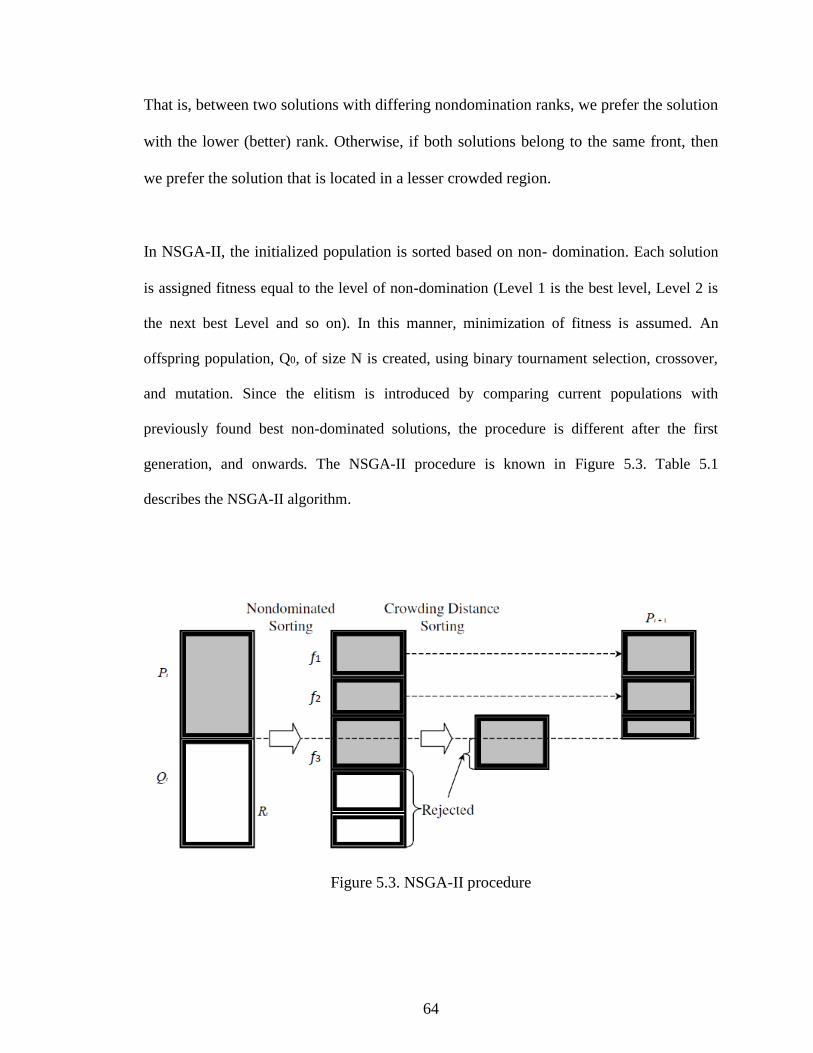
64
That is, between two solutions with differing nondomination ranks, we prefer the solution
with the lower (better) rank. Otherwise, if both solutions belong to the same front, then
we prefer the solution that is located in a lesser crowded region.
In NSGA-II, the initialized population is sorted based on non- domination. Each solution
is assigned fitness equal to the level of non-domination (Level 1 is the best level, Level 2 is
the next best Level and so on). In this manner, minimization of fitness is assumed. An
offspring population, Q0, of size N is created, using binary tournament selection, crossover,
and mutation. Since the elitism is introduced by comparing current populations with
previously found best non-dominated solutions, the procedure is different after the first
generation, and onwards. The NSGA-II procedure is known in Figure 5.3. Table 5.1
describes the NSGA-II algorithm.
Figure 5.3. NSGA-II procedure

65
Table 5.1. NSGA-II Elitism Procedure
ttt QPR
f=fast-nondomimated-sort( tR )
1tP =0 and i=1
Until NfP it 1
Crowding-distance-assignment( if )
itt fPP 11
i=i+1
sort( nif , )
)](:1[ 111 titt PNfPP
1tQ =make-new-pop( 1tP )
t=t+1
The NSGA-II algorithm is simple and straightforward. First, a combined population
ttt QPR is formed. The population tR is of size 2N. Then, the population tR is sorted
according to nondomination. Since all previous and current population members are
included in tR , elitism is ensured. Now, solutions belonging to the best nondominated set
1f are of best solutions in the combined population and must be emphasized more than
any other solution in the combined population. If the size of 1f is smaller then N, we
definitely choose all members of the set 1f for the new population 1tP . The remaining
members of the population 1tP are chosen from subsequent nondominated fronts in the
order of their ranking. Thus, solutions from the set 2f are chosen next, followed by
solutions from the set 3f , and so on. This procedure is continued until no more sets can
be accommodated. Say that the set kf is the last nondominated set beyond which no
other set can be accommodated. In general, the count of solutions in all sets from 1f to

66
kf would be larger than the population size. To choose exactly N population members,
we sort the solutions of the last front kf using the crowded-comparison operator n in
descending order and choose the best solutions needed to fill all population slots. The
new population 1tP of size N is now used for selection, crossover, and mutation to create
a new population 1tQ of size N. The individuals are selected by using a binary
tournament selection with crowed-comparison-operator. Real-coded GAs use Simulated
Binary Crossover (SBX) operator for crossover and polynomial mutation. Figure 5.4
shows the flow chart of the NSGA-II algorithm.
Comparing with NSGA, the overall complexity of the algorithm and the computation
burden of NSGA-II has reduced from O(pN3) of NSGA to O(pN
2), which is governed by
the nondominated sorting part of the algorithm.
5.4 NSGA-II Objective Functions
The power split PHEV rule-based control strategy optimization is a multi-objective
problem which has two major objectives under the constraints. The mathematical
description of the multi-objective optimization problems is as follows:
Optimization objectives of the PHEV powertrain are to reduce the fuel consumption cost
and the electricity cost. Two functions about the fuel consumption cost and the electricity
cost can be expressed as:

67
Figure 5.4. The flowchart of multi-objective optimization algorithm of NSGA-II
1
0
1
0
min
min
N
k Grid
Battelectricelec
N
kfuelfuelfuel
Pf
Pf
(5.2)
where,
),,,
,,,(,
_____arg_
arg_maxmin
lauehighoptelowopteedischm
echgelecfuel SOCSOCfff
(5.3)

68
Generally, the constraints of multi-objective problems for the power split PHEV include
the vehicle performance, such as accelerating ability and gradeability, and energy balance
between energy sources and sinks of PHEV. This study mainly focuses on the PHEV
energy management and operation cost, so the constraint considered in this study is as
follows:
GMedem PPPP (5.4)
The optimization parameters of multi-objective problems for the power split PHEV in
Table II have a critical influence over PHEV fuel economy and operation cost. The
parameters of PHEV and their range are listed follows:
6.03.0 min SOC
9.07.0 max SOC
1.17.0 arg_ echg
8.07.0 arg_ edischm
7.04.0 __ lowopte
1.19.0 __ highopte
12501010 _ laue
In this study, the population N is initially set to 20. The initialized population is sorted
based on non-domination. The total generation of NSGA-II algorithm is set to 100. The
crossover probability is 0.9 and the mutation probability is 0.01. When the generation
meets the criteria, the final populations and related objectives will be obtained.

69
5.5 Simulations
This section presents the rule-based control strategy parameters optimization results
through the different driving cycles and the PSD ratios effects to the vehicle operation
cost based on the optimization results. Two typical driving cycles - UDDS and HWFET
driving cycles are used in the simulation. Two driving cycles specification can be found
in appendix B. The influence of different numbers of the driving cycles on the rule-based
control strategy parameters are studied through the simulations. Following are driving
cycles schedule during the simulation to evaluate the driving cycle numbers effects to the
operation costs including fuel consumptions and electricity costs:
CASE I: UDDS – 1, 2, 3 driving cycles.
CASE II: HWFET – 1, 2, 3 driving cycles.
5.5.1. Baseline simulation
The baseline of the PHEV rule-based control strategy parameters is shown in Table 4.3.
The fuel consumptions and total operation costs for 1 UDDS driving cycle, 2 UDDS
driving cycles, 3 UDDS driving cycles, 1 HWFET driving cycle, 2 HWFET driving
cycles and 3 HWFET driving cycles are listed in Table 5.2.
5.5.2. Objective optimization for PSD gear ratio =3.0
The PHEV control strategy parameter optimization is carried out according to the
parameters setting given in Chapter 4.4. The PSD gear ratio is set to 3.0. Table 5.7 only
shows the optimization results of 3 HWFET driving cycles. The Pareto optimal results for

70
1 UDDS driving cycle, 2 UDDS driving cycles, and 3 UDDS driving cycles are shown in
Figure 5.5. The Pareto optimal results for 1 HWFET driving cycle, 2 HWFET driving
cycles and 3 HWFET driving cycles are shown in Fig 5.6.
The purpose of NSGA-II is to find a bunch of trade-off solutions which are termed
optimal. However, there also exist a number of poor schemes that can be substituted by
other superior ones whose objectives are non-inferior to, and at least one objective better
than theirs. From Table 5.3, the total costs of all of the Pareto optimal solutions are less
than 0.898 (USD) which is the baseline total cost. 17 Pareto optimal solutions have the
better fuel consumptions than 661.25 g, which is the baseline fuel consumption. This
means that most of the Pareto solutions are better than the baseline. Better here means
both of the objectives are smaller than the baseline. Though this fact cannot sufficiently
demonstrate that the 20 solutions are true Pareto solutions, it does demonstrate that the
solutions are at least better than the baseline.
The range of each objective in the Pareto set for 3 HWFET driving cycles is as follows:
Fuel Consumption: [510, 655] g.
Total operation cost: [0.6606, 0.7414] (USD).
Figure 5.5 and 5.6 show the relationships between the fuel consumption and electricity
cost as the distribution of the Pareto optimal solutions with the different driving cycles,
when PSD is 3.0. A set of alterative optimal PHEV parameter solutions can be obtained.
In order to compare with the baseline, the best total operation cost and best fuel

71
consumption of the Pareto results for the UDDS and HWFET driving cycle with the
different numbers of driving cycles are listed in Table 5.4 and 5.5, respectively.
For the UDDS driving cycles, when considering the best operation cost solution only, the
operation costs reduce 2.98%, 2.82%, and 2.74%, respectively, for 1 UDDS driving cycle,
2 UDDS driving cycles, 3 UDDS driving cycles. The fuel consumption increases 5.35%
and 3.58% for 2 UDDS driving cycles and 3 UDDS driving cycles, although it reduces
27.12% for 1 UDDS driving cycle. When considering the best fuel consumption solution
only, both fuel consumption and the operation cost reduce for 1 UDDS driving cycle, 2
UDDS driving cycles, and 3 UDDS driving cycles. The fuel consumptions reduce
27.12%, 3.53%, and 3.62%. The operation costs reduce 2.98%, 1.94%, and 2.53%,
respectively, for 1 UDDS driving cycle, 2 UDDS driving cycles, and 3 UDDS driving
cycles.
For the HWFET driving cycles, when considering the best operation cost solution only,
the operation costs reduce 24.22%, 25.04%, and 26.5%, respectively, for 1 HWFET
driving cycle, 2 HWFET driving cycles, and 3 HWFET driving cycles. The fuel
consumption increases 797.25% and 4.9% for 1 HWFET driving cycle and 2 HWFET
driving cycles, although it reduces 11.17% for 3 HWFET driving cycles. When
considering the best fuel consumption solution only, both fuel consumption and the
operation costs reduce for 1 HWFET driving cycle, 2 HWFET driving cycles, and 3
HWFET driving cycles. The fuel consumptions reduce 6.07%, 21.64%, and 22.87%. The
operation costs reduce 0.00%, 11.58%, and 18.26%, respectively, for 1 HWFET driving
cycle, 2 HWFET driving cycles, and 3 HWFET driving cycles.

72
Based on the analysis above, the conclusion can be made that the fuel consumption is the
critical objective to determine which Pareto optimal solutions will be chosen as the final
setting parameters.
5.5.3. Control strategy parameters optimization for PSD gear ratio =3.0
Although the optimal control strategy parameters are different with the different driving
cycles, the trends to setup the parameters still can be obtained.
For HWFET driving cycles, in order to get the best fuel consumptions, the ranges
between maximum SOC and minimum SOC are 0.6, 0.599, and 0.552, respectively for 1
HWFET driving cycle, 2 HWFET driving cycles, and 3 HWFET driving cycles.
However, in order to have the best total operation cost, the ranges between maximum
SOC and minimum SOC are 0.212, 0.208, and 0.233, respectively. The desired generator
charge torque will be higher to get the best fuel consumption, compared to the torque for
the best total operation cost. However, the desired motor discharge torque and the desired
engine lowest torque will be lower to get the best fuel consumption. The engine’s lowest
speed is almost same for the best operation cost and the best fuel consumption.
For the UDDS driving cycles, the best operation cost and the best fuel consumption
achieve the best simultaneously for 1 UDDS driving cycle. But for 2 UDDS driving
cycles and 3 UDDS driving cycles, the optimal control strategy parameters have the same
trend as the HWFET driving cycles.

73
Most researchers only used 1 driving cycle to optimize the control strategy parameters of
HEV by using GA, because they assume that the number of driving cycles will not affect
the control strategy parameters. But for PHEV, the number of driving cycles will
obviously influence the control strategy parameters. When determining the control
strategy parameters, at least three driving cycles should be considered based on the
battery capacity in this study.
Table 5.2. PHEV Operations Costs and Fuel Consumptions with Baseline Rule–
based Control Strategy
Item 1 UDDS 2 UDDS 3 UDDS 1 HWT. 2 HWT. 3 HWT.
Baseline Total Cost($) 0.235 0.568 0.949 0.289 0.587 0.898
Baseline Fuel(g) 46.13 309.53 714.81 14.16 330.65 661.25

74
Table 5.3. Objectives of the Output – 20 Tradeoff Solutions for 3 HWFET Driving
Cycles
No. SOCmax SOCmin αg_charge αm_discharge αe_opt_low αe_opt_high αωe_lau Fuel Cons.(g) Elec. Cost($US) Total Cost($US)
1 0.8931 0.3415 0.7000 0.7267 0.5655 1.0915 0.8622 587.4029 0.2546 0.7344
2 0.7000 0.6000 0.7123 0.7808 0.6262 1.0012 0.8500 617.2907 0.0464 0.7133
3 0.7000 0.4673 0.7195 0.7000 0.7000 1.0547 0.8509 604.2579 0.1079 0.6606
4 0.7000 0.5996 0.7113 0.7772 0.6221 1.0027 0.8500 628.7101 0.0471 0.6801
5 0.8752 0.3719 0.7061 0.7000 0.5449 1.1000 0.8500 672.7689 0.2324 0.7399
6 0.8318 0.5050 0.7196 0.7552 0.6212 1.0994 0.8509 651.4669 0.1513 0.6844
7 0.8215 0.5084 0.7201 0.7626 0.6224 1.0993 0.8500 655.2454 0.1450 0.6903
8 0.8422 0.4036 0.7084 0.7028 0.6158 1.0975 0.8532 639.8811 0.2026 0.7150
9 0.7003 0.5230 0.7511 0.7004 0.6921 1.0582 0.8752 566.531 0.0822 0.6843
10 0.8088 0.4172 0.7158 0.7047 0.6128 1.0961 0.8549 667.3826 0.1810 0.7077
11 0.7044 0.5766 0.7510 0.7000 0.7000 1.0811 0.8774 616.8726 0.0593 0.6872
12 0.7039 0.5133 0.7105 0.7028 0.6995 1.0614 0.8637 579.6275 0.0882 0.6798
13 0.8324 0.4088 0.7083 0.7035 0.6161 1.1000 0.8531 559.7747 0.1958 0.7121
14 0.8691 0.3432 0.7001 0.7305 0.5602 1.0935 0.8618 559.4005 0.2426 0.7414
15 0.7000 0.4952 0.7112 0.7402 0.6680 1.1000 0.8500 548.7519 0.0953 0.6761
16 0.7050 0.5599 0.7304 0.7005 0.6734 1.0508 0.8689 708.7293 0.0673 0.6802
17 0.7000 0.4676 0.7193 0.7000 0.7000 1.0533 0.8509 544.5978 0.1078 0.6763
18 0.8107 0.4154 0.7159 0.7046 0.6122 1.0949 0.8549 510.0097 0.1827 0.7090
19 0.7003 0.4679 0.7194 0.7000 0.7000 1.0534 0.8518 539.349 0.1078 0.6882
20 0.7050 0.5603 0.7298 0.7005 0.6724 1.0503 0.8688 530.1569 0.0671 0.6836

75
0.00
0.05
0.10
0.15
0.20
0.25
0.00 0.10 0.20 0.30
Fuel Cost ($US)
Ele
ctri
city
Co
st (
$U
S)
(a)
0.00
0.05
0.10
0.15
0.20
0.25
0.30
0.20 0.40 0.60 0.80
Fuel Cost ($US)
Ele
ctri
city
Co
st (
$U
S)
(b)
0.00
0.05
0.10
0.15
0.20
0.25
0.30
0.60 0.80 1.00 1.20
Fuel Cost ($US)
Ele
ctri
city
Co
st (
$U
S)
(c)
Figure 5.5. NSGA-II Pareto optimal results for UDDS. (a) 1 UDDS driving cycle. (b) 2
UDDS driving cycles. (c) 3 UDDS driving cycles.

76
0.00
0.05
0.10
0.15
0.20
0.25
0.30
0.00 0.05 0.10 0.15 0.20 0.25
Fuel Cost ($US)E
lect
rici
ty C
ost
($
US
)
(a)
0.00
0.05
0.10
0.15
0.20
0.25
0.30
0.20 0.30 0.40 0.50
Fuel Cost ($US)
Ele
ctri
city
Co
st (
$U
S)
(b)
0.00
0.05
0.10
0.15
0.20
0.25
0.30
0.45 0.55 0.65
Fuel Cost ($US)
Ele
ctri
city
Co
st (
$U
S)
(c)
Figure 5.6. NSGA-II Pareto optimal results for HWFET: (a)1 HWFET driving cycle. (b)
2 HWFET driving cycles. (c) 3 HWFET driving cycles.

77
Table 5.4. PHEV NSGA-II Simulation Results in UDDS Driving Cycles – Control
Strategy Parameters and Operations Costs
Item Best Total Costs Best Fuel Consumptions
1 UDDS 2 UDDS 3 UDDS 1 UDDS 2 UDDS 3 UDDS
SOCmax 0.869 0.894 0.863 0.869 0.900 0.900
SOCmin 0.443 0.364 0.373 0.443 0.300 0.300
αg_charge 0.794 0.877 0.920 0.794 0.867 0.998
αm_discharge 0.800 0.799 0.794 0.800 0.710 0.800
αe_opt_low 0.561 0.572 0.700 0.561 0.668 0.644
αe_opt_high 1.095 1.049 1.064 1.095 0.901 1.100
αωe_lau 0.850 0.851 0.951 0.850 1.100 0.917
Tot. Cost ($) 0.228 0.552 0.923 0.228 0.557 0.925
Cost Comparison 2.98% 2.82% 2.74% 2.98% 1.94% 2.53%
Fuel (g) 33.62 326.1 740.4 33.62 298.60 688.9
Fuel Comparison 27.12% -5.35% -3.58% 27.12% 3.53% 3.62%

78
Table 5.5. PHEV NSGA-II Simulation Results in HWFET Driving Cycles – Control
Strategy Parameters and Operations Costs
Item Best Total Costs Best Fuel Consumptions
1 HWT. 2 HWT. 3 HWT. 1 HWT. 2 HWT. 3 HWT.
SOCmax 0.717 0.791 0.700 0.900 0.899 0.893
SOCmin 0.505 0.583 0.467 0.300 0.300 0.341
αg_charge 0.916 0.729 0.720 1.036 0.942 0.700
αm_discharge 0.800 0.799 0.700 0.745 0.789 0.727
αe_opt_low 0.700 0.693 0.700 0.615 0.648 0.566
αe_opt_high 1.100 1.100 1.055 0.906 1.036 1.091
αωe_lau 0.850 0.852 0.851 0.850 0.852 0.862
Tot. Cost ($) 0.219 0.440 0.660 0.289 0.519 0.734
Cost Comparison 24.22% 25.04% 26.50% 0.00% 11.58% 18.26%
Fuel (g) 127.05 346.85 587.40 13.30 259.09 510.01
Fuel Comparison -797.25% -4.90% 11.17% 6.07% 21.64% 22.87%
79
5.6 Summary
The PHEV rule-based control strategy parameter optimization based on the genetic
algorithm NSGA-II was studied in this chapter. It will save the vehicle controller
calibration time and reduce the development cost to apply this approach as off-line
optimization. The main study in this chapter focused on following:
The NSGA-II objective functions were created based on the PHEV rule-based
control strategy vehicle model. The constrains of the rule-based control strategy
parameters were determined by evaluating the performance of the components
and systems. The total generation of NSGA-II algorithm is set to 100. The
crossover probability is 0.9 and the mutation probability is 0.01.
The simulations of the baseline vehicle (PSD gear ratio = 3.0) for 1, 2, and 3
UDDS and HWFET driving cycles were implemented and the optimal simulations
of the baseline vehicle at the different driving cycles also were discussed.
Comparing the optimal simulation results with the baseline, the best fuel
consumptions are improved at all of the driving cycles. However, the best total
cost only are improved at 1 UDDS driving cycle and 3 HWFET driving cycles.
80
CHAPTER 6
OPTIMAL DESIGN OF PSD GEAR RATIO
6.1 Introduction
The HEVs perfectly combine the advantages of the conventional vehicles and electric
vehicles. The power split HEVs are the highlight in the HEV family. Same as the other
vehicles, the power split device (Transmission – e-CVT) design is one of the most
important parts during the development of the power split HEV. The power split device
gear ratio is one of the most critical parameters. The basic power split device gear ratio
design is based on the vehicle performance requirements [72]. The gear ratio should
ensure the vehicle to meet the acceleration, gradeability, maximum top speed
requirements. With the development of the HEV study, the optimal methods [73], [74]
are implemented to optimize the planetary gear parameters to lower the fuel
consumption. However, because of the condition of assembly of planetary gear set, the
series gear ratios are not continuous. The simulation results cannot meet the practice
requirements.
An innovative six step design approach to optimize the PSD gear ratio to minimize the
fuel consumption and operation cost is presented in this chapter. Figure 6.1 shows the
flow chart of the design procedure. The related study from step 2 to step 5 has been
discussed in Chapter 2 to Chapter 5. This chapter will focus on step 1 and step 6.

81
Figure 6.1. Flow chat of six-step approach to design PHEV PSD gear ratio
6.2 Determination of Initial PSD Gear Ratio
Rearranging (2.10) to express the speed function of planetary gear components as
following:
crs kk )1( (6.1)
(6.1) is a plane equation, which is called the Characteristic Speed Plane (CSP), in the
Cartesian Coordinate System, r, c, s represented by the x, y and z axes, respectively
(Figure 6.2).

82
Figure 6.2. Relationship between characteristic speed plane with maximum vehicle
performance plane
The CSP shows the working range of the planetary gear. The plane A in Figure 6.2
represents the CSP, where A1A2 is located at plane abcd, which is parallel to the plane xy,
and represents the speed relationship between the carrier and the ring gear when the sun
gear is running at highest speed. A2A3 is located at plane bcgf, which is parallel to the
plane xz, and represents the speed relationship between the sun gear and the ring gear
when the carrier gear is running at highest speed. A3A4 is located at plane cdgh, which is
parallel to the plane yz, and represents the speed relationship between the carrier and the
sun gear when the ring gear is running at highest speed. Plane B was created when
r=r,max, c=c,max and s=s,max. The normal vector of plane A and B are u=[k, -(k+1),
1] and v=(2/r,max, -2/=c,max, 1/=s,max).

83
In order to have better vehicle performance, the engine and motor should have a wider
range of speed regulation. This means the smaller the angle between plane A and B is the
better the vehicle performance will be. The angle between plane A and B can be
calculated as follows:
vu
vuBA
1cos),( (6.2)
6.3 PSD Planetary Gear Ratio Numerical Analysis
6.3.1. Initial planetary gear ratio
From (6.2), the analyses to the planetary gear ratio variation with the maximum speeds of
the traction motor, the engine and the generator/motor are illustrated in Figures 6.3, 6.4
and 6.5. The optimal planetary gear ratio affects the maximum speeds of the engine, the
traction motor and the generator/motor. The optimal planetary gear ratio will be
decreased with the increase of the designed maximum traction motor speed (Figure 6.3),
the decrease of the designed maximum engine speed (Figure 6.4), and the decrease of the
designed maximum generator/motor speed (Figure 6.5).
Based on the vehicle information of Appendix I, the curve of the angle between plane A
and B with the planetary gear ratio was determined in Figure 6.6. The minimum angle is
0.03 (rad) at k=3.08. The gear ratios from 2.6 to 3.4 were considered for the further
simulation.

84
0
0.2
0.4
0.6
0.8
1
0 2 4 6 8 10
PSD Gear Ratio
An
gle
.
9000rpm
7000rpm
5000rpm
Figure 6.3. Planetary gear ratio versus maximum ring gear speed (r,max)
0
0.2
0.4
0.6
0.8
1
0 2 4 6 8 10
PSD Gear Ratio
An
gle
.
4000rpm
5000rpm
6000rpm
Figure 6.4. Planetary gear ratio versus maximum carrier speed (c,max)

85
0
0.2
0.4
0.6
0.8
1
0 2 4 6 8 10PSD Gear Ratio
An
gle
.8000rpm
10000rpm
12000rpm
Figure 6.5. Planetary gear ratio versus maximum sun gear speed (s,max)
0
0.2
0.4
0.6
0.8
1
0 2 4 6 8 10
PSD Gear Ratio
An
gle
.
Figure 6.6. Initial PSD gear ratio

86
6.4 Planetary Gear Condition of Assembly
Consideration of the condition of assembly [75], the determination of the tooth number of
the planetary gear train will be based on the gear ratio. Assuming that the ring gear is
fixed when designing the tooth number of the planetary gear train, the sun gear is the
driving gear, and the carrier is the driven component. From equation (2.10), the gear ratio
between the sun gear and the carrier i is:
i=1+k (6.3)
The relationship between the tooth number of planetary gear train – Zs, Zr, and Zc – is:
s
src Z
iZZZ
2
1
2
(6.4)
Based on the condition of assembly:
C
n
ZZ sr (6.5)
Combining the equations from (6.3) to (6.5):
n
ii
iCZZZ rcs :)1(:
2
2:1:::
(6.6)
Table 6.1. shows all of the gear ratio which meet the equation (6.6) from k=2.6 to k=3.4.
Table 6.1. The Tooth Number Which Meet the Condition of Assembly From Gear
Ratio 2.6 to 3.4
k C Za Zb Zc
2.60 24 20 52 16
2.75 20 16 44 14
2.90 26 20 58 19
3.00 24 18 54 18
3.20 28 20 64 22
3.25 34 24 78 27
3.40 22 15 51 18

87
6.5. PSD Gear Ratio Optimization Design
The optimization simulations of the power split PHEV at different gear ratios are carried
out through NSGA-II for the UDDS and HWFET driving cycles. The different numbers
of the driving cycles are used in the simulations to evaluate the influence on the rule-
based control strategy parameters. Following are driving cycles used during the
simulation to evaluate the driving cycle numbers effects to the operation costs including
fuel consumptions and electricity costs at different planetary gear ratios between 2.6 to
3.4:
CASE I: UDDS – 1, 2, 3 driving cycles.
CASE II: HWFET – 1, 2, 3 driving cycles.
Based on the driving cycle numbers and the gear ratios from 2.6 to 3.4, the simulation
matrix is set up. Figure 6.7- Figure 6.12 show the simulation results.
For 1 UDDS driving cycle, both fuel consumptions and operation costs decrease with the
increase of gear ratios. For 2 UDDS driving cycles, the fuel consumptions decrease with
the increase of the gear ratios. However, both of the lowest operation costs and fuel
consumptions still are at gear ratio 3.4. For 3 UDDS driving cycles, the lowest economy
fuel consumption and operation cost can be found at gear ratio 2.9.
For 1 HWFET driving cycle, both fuel consumption and operation costs have the same
trend as the UDDS driving cycles, as they decrease with the increase of the gear ratio. For
2 and 3 UDDS driving cycles, the economy fuel consumption can be found at gear ratio
3.0 and 3.2, respectively. The economy operation costs are shown at gear ratio 3.25 or 3.4.

88
Table XI shows the differences of the maximum and minimum optimal fuel
consumptions between gear 2.6 and 3.4. When the number of driving cycles increases,
the difference also increases. This is because the vehicle was run at CD mode at the first
or first and a half driving cycle, and CS mode at the third driving cycle.
From the simulation results above, the designed all electric operation range (AEOR) will
influence the PSD gear ratio selection. In other word, the battery capacity will influence
the PSD gear ratio selection. If the designed AERO is larger and the more battery
capacity will be chosen, the higher PSD gear ratio will be selected. If the designed AERO
is lower and the less battery capacity will be chosen, the lower PSD gear ratio will be
selected.
However, the PSD planetary gear design is a trade-off process. When designing a power
split PHEV planetary gear, not only are the fuel consumption and operation costs
considered, but also the vehicle performance, emission, gear weight, strength, standards
etc.
Table 6.2. The Differences of the Maximum and Minimum Fuel consumptions at
Gear Ratio 2.6 to 3.4
# of Driving Cycle 1 2 3
UDDS 3.40 11.35 25.89
HWFET 2.54 27.85 62.28

89
31
32
33
34
35
36
37
2.6 2.75 2.9 3 3.2 3,25 3.4
Gear Ratio
Fuel
Consu
mptions
(g)
(a)
0.2260
0.2265
0.2270
0.2275
0.2280
0.2285
0.2290
0.2295
0.2300
0.2305
2.6 2.75 2.9 3 3.2 3,25 3.4
Gear Ratio
Op
erat
ion
Co
st($
US
)
(b)
Figure 6.7. Fuel consumption and operation cost for 1 UDDS driving for various PSD
gear ratios. (a) Best fuel consumptions. (b) Best operation costs.

90
290
292
294
296
298
300
302
304
306
308
310
2.6 2.75 2.9 3 3.2 3,25 3.4
Gear Ratio
Fuel
Consu
mptions
(g)
(a)
0.5300
0.5350
0.5400
0.5450
0.5500
0.5550
0.5600
2.6 2.75 2.9 3 3.2 3,25 3.4
Gear Ratio
Op
erat
ion
Co
st (
$U
S)
(b)
Figure 6.8. Fuel consumption and operation cost for 2 UDDS driving cycle for various
PSD gear ratios. (a) Best fuel consumptions. (b) Best operation costs.

91
665
670
675
680
685
690
695
700
705
710
2.6 2.75 2.9 3 3.2 3,25 3.4
Gear Ratio
Fuel
Consu
mptions
(g)
(a)
0.9050
0.9100
0.9150
0.9200
0.9250
0.9300
0.9350
0.9400
2.6 2.75 2.9 3 3.2 3,25 3.4
Gear Ratio
Op
erat
ion
Co
st (
$U
S)
(b)
Figure 6.9. Fuel consumption and operation cost for 3 UDDS driving cycles for various
PSD gear ratios. (a) Best fuel consumptions. (b) Best operation costs.

92
0
2
4
6
8
10
12
14
16
2.6 2.75 2.9 3 3.2 3,25 3.4
Gear Ratio
Fuel
Consu
mptions
(g)
(a)
0.2000
0.2050
0.2100
0.2150
0.2200
0.2250
0.2300
0.2350
0.2400
2.6 2.75 2.9 3 3.2 3,25 3.4
Gear Ratio
Op
erat
ion
Co
st($
US
)
(b)
Figure 6.10. Fuel consumption and operation cost for 1 HWFET cycle for various PSD
gear ratios. (a) Best fuel consumptions. (b) Best operation costs.

93
200
220
240
260
280
300
320
340
2.6 2.75 2.9 3 3.2 3,25 3.4
Gear Ratio
Fuel
Consu
mptions
(g)
(a)
0.4100
0.4200
0.4300
0.4400
0.4500
0.4600
0.4700
0.4800
2.6 2.75 2.9 3 3.2 3,25 3.4
Gear Ratio
Op
erat
ion
Co
st (
$U
S)
(b)
Figure 6.11. Fuel consumption and operation cost for 2 HWFET driving cycles for
various PSD gear ratios. (a) Best fuel consumptions. (b) Best operation costs.

94
450
460
470
480
490
500
510
520
530
540
550
2.6 2.75 2.9 3 3.2 3,25 3.4
Gear Ratio
Fuel
Consu
mptions
(g)
(a)
0.6200
0.6300
0.6400
0.6500
0.6600
0.6700
0.6800
0.6900
0.7000
0.7100
0.7200
2.6 2.75 2.9 3 3.2 3,25 3.4
Gear Ratio
Op
erat
ion
Co
st (
$U
S)
(b)
Figure 6.12. Fuel consumption and operation cost for 3 HWFET driving cycles for
various PSD gear ratios. (a) Best fuel consumptions. (b) Best operation costs.

95
6.6 Summary
An innovative PSD gear ratio design approached of the single mode power split PHEV
was presented in this chapter. The NSGA-II algorithm was used to optimize the rule-
based control strategies parameters at the different diving cycles and different gear ratios.
An important conclusion obtained is that the designed AEOR is the key parameter to
determine the PSD gear ratio. The main study in this chapter focused on following:
The initial PSD gear ratio determination was presented. It was based on the main
power sources maximum speed to ensure the engine and motor to have the wider
operation ranges.
The condition of assembly of PSD planetary gear was discussed and the available
gear ratios were analysed at a reasonable range.
The fuel consumptions and operation costs were simulated by NSGA-II, therefore
determining the best PSD gear ration to minimum the PHEV fuel consumption
and operation cost.
From the above chapters discussed, the innovative PSD gear ratio design approached of
the single mode power split PHEV can be summarized as following :
Step 1 – Designing the initial planetary gear ratio of PHEV: the gear ratio range
was be determined based on the vehicle performance requirements.
Step 2 – Modeling the vehicle systems: the dynamic PSD and powertrain models
were used for the PHEV energy management simulations.
Step 3 – Determining the ideal PHEV control strategy: DP was employed to
optimize the control strategy.
96
Step 4 – Developing the real time control strategy: the rule based control strategy
was developed based on DP simulation results:
Step 5 – Optimizing the rule-based control strategy parameters: NSGA-II was
used to optimize the rule-based control parameters.
Step 6 – Determining the final PHEV planetary gear ratio: two typical driving
cycles - the UDDS and HWFET - were used to determine the PSD gear ratio.

97
CHAPTER 7
CONCLUSIONS AND FUTURE WORKS
7.1 Summary and Conclusion
The main objective of this study was to present an innovative design approach to
optimize the single mode power split PHEV PSD gear ratio to minimize the vehicle fuel
consumption and operation cost in this thesis.
The works that have been done on this research and main conclusions are summarized as
follows:
The backward-looking power split PHEV model was effectively created under the
Matlab environment based on the power source testing results. It provided a
simulation platform for the vehicle control strategy development. The interaction
between the sub-systems can be analyzed, the vehicle performance, such as fuel
economy and drivability, can be evaluated, the components size also can be
studied by using this vehicle model. The model accurate is enough for the energy
consumption simulations. It also laid the solid foundation for the close-loop
forward looking vehicle model simulation.
The DP optimal control model of PHEV was created under the condition of given
driving cycles to optimize the vehicle fuel consumption and operation cost. The
state variable of the optimal control model is SOC, the control variables are the
motor and generator torques. The step was determined based on the given driving
cycles. The assumption was made that the vehicle consumption is constant within
each steps, therefore changing the continuous optimal control to a series of sub-

98
problems. The optimal control strategy was obtained by the DP approach. The
purpose of this study is to determine the global optimal fuel consumption and
operation cost as the benchmark of the real-time PHEV control strategy.
The rule-based PHEV control strategy was developed by studying the vehicle
operation modes. The control strategy parameters were determined based on the
engine, motor, battery internal resistance, and the DP simulation results.
Comparing with the fuel consumption based on the DP simulation results, the fuel
consumption increases 12.98%.
The multi-objective optimal model for the PHEV rule-based control strategy
parameters was presented based on the non-dominated sorting genetic algorithm
(NSGA-II). The control strategy parameters were optimized by using the
backward looking vehicle model to calculate the objectives and constrains. The
simulation results show that the optimized rule-based control strategy can reduce
the vehicle fuel consumption 3.53% for 2 UDDS driving cycles and 21.64% for 2
HWFET driving cycles.
An innovative design method for the single mode power split PHEV PSD gear
ratio was discussed. The purpose of this study is to find an approach to design the
PSD gear ratio by considering the vehicle performance and fuel consumptions.
The significant of this method is not only improve vehicle performance and fuel
consumptions, but also to reduce the vehicle PSD development time and save the
cost.

99
7.2 Future Works
The PHEV technology is still a new area for the automotive industry. There are many
problems to be solved in the future. For this study, the further research is as following:
Forward-looking vehicle model development: In order to describe the vehicle
operate in the real conditions, the forward looking vehicle model should be
developed. The forward looking vehicle model is a close loop control system,
including the driver model to simulate the actions of brake and acceleration
pedals. The model should include the transient characteristics of the sub-system,
such as clutches on and off. Some sub-system model should be improved. The
engine emission did not consider in this study. The future work should consider
the engine fuel consumption and emissions.
Adaptive control strategy study: Because the driver operations and road
conditions are random, it is difficult to apply the specific driving cycle optimal
control strategy to the actual vehicle. In order to simulate the random driver
operations and road conditions, the fuzzy control logic or neural network can be
used. The real time on line recognition function to the driver intention, driving
cycle characteristic parameters should be considered in the control strategy.

100
APPENDICES
APPENDIX A PHEV Vehicle Specification
Table A.1. PHEV Vehicle Specification
Vehicle Mass [kg] Coefficient of Aerodynamic
Drag
Frontal Area of Vehicle
[m2]
1,250 0.30 2.52
Wheel Radius [m] Coefficient of Rolling
Resistance Air Density [kg/m
3]
0.287 0.015 1.184
Engine
Max Power [kW] Max torque [Nm] Max Speed [rpm]
57 @ 4,500 rpm 111 @ 4,200 rpm 5,000
Motor I
Rated Power [kW] Rated Torque [Nm] Max Speed [rpm]
35 @ 940 to 2,000
[rpm] 305 @ 0 to 940 [rpm] 7,000
Motor II
Rated Power [kW] Rated Torque [Nm] Max Speed [rpm]
15 60 11,000
Battery
Voltage [V] Capacity [Ah]
312 13

101
APPENDIX B UDDS and HWFET Driving Cycles
0 500 1000 15000
5
10
15
20
25
30
Time
Vehic
le S
peed (
m/s
)
Urban Dynamometer Driving Schedule (UDDS)
Figure B.1. Urban dynamometer drive schedule (UDDS) driving cycle
0 100 200 300 400 500 600 700 8000
5
10
15
20
25
30
Time
Veh
icle
Spe
ed (
m/s
)
Highway Fueleconomy Driving Schedule (HWFET)
Figure B.2. Highway fuel economy drive schedule (HWFET) driving cycle

102
Table B.1. Driving Cycles Specification
Driving cycle UDDS HWFET
Max. Speed (km/h) 91.24 96.39
Ave. Speed (km/h) 31.53 76.27
Distance (km) 11.99 16.51
Time (s) 1369 779

103
REFERENCES
1. U.S. Environmental Protection Agency, “INVENTORY OF U.S. GREENHOUSE
GAS EMISSIONS AND SINKS: 1990 – 2009”, EPA 430-R-11-005 APRIL 15,
2011
2. http://www.eia.gov/
3. D. Bennett, “Zero Emission Vehicles: The Air Pollution Messiah? Northeastern
States Mandate ZEVs Without Considering the Alternatives or Consequences”,
Volume 20, William & Mary Environmental Law & Policy Review, 1996.
4. www.afdc.energy.gov/afdc/data/
5. http://www.afdc.energy.gov/
6. K.Morita, “Automotive power source in 21st century,” JSAE Review, 2003, 24(1):
3-7
7. K. Okamoto, “Overview of current and future hybrid technology,” Proc of the
Symposium on Advanced Automotive Powerplants and Energy Resources,
Beijing: China SAE, 2002. 89-94
8. C. Chan, “The state of the art of electric and hybrid vehicles,” Proc of IEEE,
2002, 90(2): 247-275
9. A.Wyczalek, “ Hybrid electric vehicles year 2000 status,” IEEE AES Systems
Magazine, 2001, 16(3): 15-19
10. W.G. Livezey, “Input-split-power, Output-split-power, Compound-split-power,
Power Train,” US Patent 3,470,769, issued Nov. 1969.
11. S. Abe, S. Sasaki, H. Matsui, K. Kubo, “Development of Hybrid System for Mass
Productive Passenger Car,” JSAE Proc. 9739543, pp. 21-24.
12. T. M. Grewe, B. M. Conlon, A. G. Holmes, “Defining the General Moto 2-Mode
Hybrid Transmission,” SAE Paper 2007-01-0273.
13. M. Schulz, “Circulating Mechnical Power in a Power-split Hybrid Electric
Vehicle Transmission,” Proc. Instn Mech. Engrs., Vol. 208, Part D: J.
Automotive Engineering, 2004.
14. http://www.getrag.de/

104
15. J. M. Miller, “Hybrid Electric Vehicle Propulsion System Architectures of the e-
CVT Type,” IEEE Transactions on Power Electronics, Vol. 21, No. 3, May,
2006.
16. D. Zhang, J. Chen, T. Tsieh, J. Rancourt, M.R. Schmidt, “Dynamic Modeling and
Simulation of Two-Mode Electric Variable Transmission,” Proc. of IMechE Vol 215,
pp. 1217-1223, 2001.
17. D. Rizoulis, J. Burl, and J. Beard, “Control Strategies for a Series-Parallel Hybrid
Electric Vehicle,” SAE Paper 2001-01-1354, 2001.
18. J. Liu, “Modelling, Configuration and Control Optimization of Power-split Hybrid
Vehicles,”Dissertation, University of Michigan.
19. R. Zanasi, and F. Grossi, “Modeling and control of Power-split Hybrid electric
Vehicle,” In Proc. Of IEEE Vehicle Power and Propulsion Conference (VPPC),
Sept. 1-3, 2010
20. J. Wishart, Y. Zhou, Z. Dong, and F. Firmani, “Dynamic Modeling and
Simulation of a multi-regime Hybrid Vehicle Powertrain Architecture,” Proc. Of
International Journal of Electric and Hybrid Vehicles, Vol. 1 Page 188-219, 2008
21. M. P. O’Keefe and T. Markel, “Dynamic programming applied to investigate
energy management strategies for a plug-in HEV,” National Renewable Energy
Lab., CO, Report No. NREL/CP- 540-40376, 2006.
22. C.-C. Lin, H. Peng, and J. Grizzle, “A stochastic control strategy for hybrid
electric vehicles,” in Proceedings of the American Control Conference, 2004.
23. B. Bole, S. Coogan, C. Cubero-Ponce, D. Edwards, R. Melsert, D. Taylor, “
Energy Management Control of a Hybrid Electric Vehicle with Two-Mode
Electrically Variable Transmission,” EVS26 International Battery, Hybrid and
Fuel Cell Electric Vehicle Symposium, Los Angeles, California, May 6 - 9, 2012
24. S. Moura, H. Fathy, D. Callaway, J. Stein, “A Stochastic Optimal Control
Approach for Power Management in Plug-In Hybrid Electric Vehicles” IEEE
Trans. Contr. Sys. Techn. 19(3): 545-555, 2011
25. C-C. Lin, H. Peng, J.W. Grizzle, “Power management strategy for a parallel
hybrid electric truck,” IEEE Transactions on Control Systems Technology, 2003,
11 (6): 839-849

105
26. N. Kim S. Cha, and H. Peng, “Optimal Control of Hybrid Electric Vehicles Based
on Pontryagin’s Minimum Peinciple,” IEEE Transactions on Control System
Technology, Vol. 19, No. 5, 1279-1287, September 2011.
27. L. Serrao, G. Rizzoni, “Optimal Control of Power Split for a Hybrid Electric
Refuse Vehicle,” in Proc. 2008 American Control Conf., Seattle, WA, 2008, pp
4498-4503.
28. G. Rousseau, D. Sinoquet, P. Rouchon, “Constrained Optimization of Energy
Management for a Mild-Hybrid Vehicle,” Oil-Gas Science and Technology, IFP,
Vol. 62, No. 4, 2007, pp. 623-624.
29. X. Wei, L. Guzzella, V. I. Utkin, G. Rizzoni, “Model-Based Fuel Optimal Control
of Hybrid Electric Vehicle Using of Hybrid Electric Vehicle Using Variable
Structure Control Systems,” ASME J. Dynamic Syst., Meas., Control, vol. 129,
No. 1, January 2007, pp. 13-19.
30. C. Kim, E. NamGoong, and S. Lee, “Fuel Economy Optimization for Parallel Hybrid
Vehicles with CVT,” SAE Paper 1999-01-1148, 1999.
31. G. Paganelli, T.M. Guerra, S. Delprat, J.J. Santin, M. Delhom, E. Combes,
“Simulation and Assessment of Power Control Strategies for a Parallel Hybrid Car,”
J. Automobile Engineering, also in Proc. Of the Institution of Mechanical Engineers
IMechE, SAE International, 214, pp. 705-718, 2000.
32. G. Paganelli, G. Ercole, A. Brahma, Y. Guezennec, G. Rizzoni, “General Supervisory
Control Policy for the Energy Optimization of Charge-Sustaining Hybrid Electric
Vehicles,” JSAE Review, Vol. 22, No. 4, pp. 511-518, 2001.
33. G. Paganelli, M. Tateno, A. Brahma, G. Rizzoni, and Y. Guezennec,
“ContrDevelopment for a Hybrid-Electric Sport-Utility Vehicle: Strategy,
Implementation and Field Test Results,” Proceedings of the American Control
Conference, Arlington, VA, 2001.
34. C. Musardo, G. Rizzoni, and B. Staccia, “A-ECMS: An Adaptive AlgoHybrid
Electric Vehicle Energy Management,” Proc. of IEEE Conference on Decision and
Control, Seville, Spain, 2005.
35. H. Banvait, X. Lin, S. Anwar, and Y. Chen, “Plug-in Hybrid Electric Vehicle
Energy Management System Using Particle Swarm Optimization,” World Electric
Vehicle Journal, Vol. 3 - ISSN 2032-6653, 2009.
36. J. Liu and H. Peng, “Modeling and Control of Power-split Hybrid Vehicle,” IEEE
Transactions on Control System Technology, Vol. 16, No. 6, November 2008.

106
37. J. Liu, and H. Peng, “Control Optimization for a Power-Split Hybrid Vehicle,”
Proceedings of the 2006 American Control Conference, Minneapolis, MN, 2006.
38. K. L. Butler, K. M. Stevens, M. Ehsani, “A versatile computer simulation tool for
design and analysis of electric and hybrid drive trains,” SAE Paper 970199, 1997.
39. M. R. Cuddy, K. B.Wipke, “Analysis of the fuel economy benefit of drivetrain
hybridization,” SAE Paper 970289, 1997.
40. K. B. Wipke, M. R. Cuddy, and S. D. Burch, “ADVISOR 2.1: A user-friendly
advanced powertrain simulation using a combined backward/forward approach,”
IEEE Trans. Vehicular Technol., vol. 48, no. 6, pp. 1751–1761, Nov. 1999.
41. T. Markel, A. Brooker, T. Hendricks, V. Johnson, K. Kelly, B. Kramer, M.
O’Keefe, S. Sprik, and K.Wipke, “ADVISOR: A systems analysis tool for
advanced vehicle modeling,” J. Power Sources, vol. 110, no. 2, pp. 255–266,
Aug. 2002.
42. “PSAT Training,” http://www.anl.gov/
43. http://www.powersimtech.com/
44. http://vtb.engr.sc.edu/vtbwebsite/#/Overview
45. Won, J. S., Langari, R., and Ehsani, M., (2005), “An Energy Management and
Charge Sustraining Strategy for a Parallel Hybrid Vehicle With CVT,” IEEE
Transactions on Control System Technology, Vol. 13, No. 2, pp. 313-320.
46. P. Pisu, G. Rizzoni, C. Musardo, and B. Staccia, “A Comparative Study of
Su;ervisory Control Strategies for Hybrid Electric Vehicles,” Proc. Of International
Mechanical Engineering Congress and Exposition, Anaheim, CA, 2004.
47. R. Bellman, “Dynamic Programming,” Princeton University Press, 1957.
48. C.-C. Lin, H. Peng, J. Grizzle, and J.-M. Kang, “Power management strategy for a
parallel hybrid electric truck,” IEEE Transactions on Control Systems
Technology, vol. 11, no. 6, pp. 839–849, 2003.
49. http://www.eia.doe.gov
50. P. Rutquist, “Optimal control for the energy storage in a hybrid electric vehicle,”
Proceedings of the 19th International Electric Vehicle Symposium, Busan, Korea,
2002. 1133-1139
51. R. E. Larson, J. L. Casti, “Principles of dynamic programming. Part I: Basic
analytic and computational methods,” New York: Marcel Dekker, Inc. 1978

107
52. D. P. Bertsekas, Dynamic Programming and Optimal Control. Belmont, MA:
Athena Scientific, 1995.
53. A. P. De Madrid, S. Dormido, F. Morilla, “Reduction of the dimensionality of
dynamic programming: a case study,” Proc. American Control Conference, San
Diego, California, USA, 1999. 2852-2856
54. R. Luus, “Optimal control by dynamic programming using systematic reduction
in grid size,” Int. Journal of Control, 1990, 51(5): 995-1013
55. N. Jalil, A. Kheir and M. Salman, “A Rule-Based Energy Management Strategy
for a series Hybrid Vehicle”, Proc. of American Control conference, pp. 689-693,
June 1997.
56. B. Harpreetsingh, S. Anwar, Y. Chen, “A Rule-based Energy Management
Strategy for Plug-in Hybrid Electric Vehicle (PHEV),”in Proc. of the American
Control Conference, St. Louis. USA, June 10-12, 2009.
57. V. Johnson, K. Wipke, D. Rausen, “HEV Control Strategy for Real-Time
Optimization of Fuel Economy and Emissions”, SAE Technical Paper 2000-01-
1543, 2000.
58. D. Karboeski, A. Rousseau, B. Pagerit, and P. Sharer “Plug-in Vehicle Control
Strategy: From Global Optimization to Real-time Application,” in Proc. of the
EVS22, October, 2004.
59. N. Schouten, M. Salman, N. Kheir, “Fuzzy logic control for parallel hybrid
vehicles,” IEEE Transactions on Control Systems Technology, 2002, 10(3): 460-
468
60. A. Rousseau, S. Pagerit, and, D. Gao, “Plug-in Hybrid Electric Vehicle Control
Strategy Parameter Optimization,” Journal of Asian Electric Vehicles, Volume 6,
December 2008.
61. S. Hiramatsu, Y. Nakayama, Y. Kikuchi, “Development of the battery ECU for
the Toyota hybrid system.” Proceedings of the 15th International Electric Vehicle
Symposium, Brussels, Belgium, 1998
62. K. Kelly, A. Rajagopalan, “Benchmarking of OEM hybrid electric vehicles at
NREL,” Technical Report NREL/TP-540-31086, National Renewable Energy
Laboratory, USA, 2001

108
63. Y. Zhu, Y. Chen, G. Tian, H. Wu, Q. Chen, “A Four-step Method to Design an
Energy Management Strategy for Hybrid Vehicles”, Proceeding of the 2004
American Control Conference, Boston, Massachusetts June 30 - July 2, 2004
64. R. Zhang, Y. Chen, “Control of Hybrid Dynamical Systems for Electrical
Vehicles”, Proceeding of the 2004 American Control Conference, pp. 2884-2889
Vol. 4, 2001
65. A. Piccolo, L. Ippolito, V. Galdi, A. Vaccaro, “Optimization of Energy Flow
Management in Hybrid Electric Vehicles via Genetic Algorithm,” 2001 IEEE
/ASME International Conference on Advanced Intelligent Mechatronics
Proceedings, Como, Italy, July 2001.
66. C. Desai, S. Williamson, “Optimal design of a parallel Hybrid Electric Vehicle
using multi-objective genetic algorithms.” in Proc. of the IEEE Vehicle Power
and Propulsion Congress, 2009.
67. A. Wang, W. Yang, “Design of Energy Management Strategy in Hybrid Electric
Vehicles by Evolutionary Fuzzy System, Part II: Tuning Fuzzy Controller by
Genetic Algorithms,” Proceedings of the 6th World Congress on Intelligent
Control and Automation, June 21 - 23, 2006, Dalian, China.
68. M. Jain, C. Desai, N. Kharma, and S. S. Williamson, “Optimal powertrain component
sizing of a fuel cell plug-in hybrid electric vehicle using multi-objective genetic
algorithm,” in Proc. IEEE Annual Conf. of the Industrial Electronics Society, Porto,
Portugal, Nov. 2009, pp. 3741-3746.
69. B. Huang, Z. Wang, Y, Xu, “Multi-Objective Genetic Algorithm for Hybrid
Electric Vehicle Parameter Optimization,” Proceedings of the 2006 IEEE/RSJ
International Conference on Intelligent Robots and Systems, October 9 - 15, 2006,
Beijing, China
70. N. Srinivas and K. Deb. “Multiobjective Optimization Using Nondominated
Sorting in Genetic Algorithms.” Evolutionary Computation, 2(3):221 - 248, 1994
71. K. Deb, A. Pratap, S. Agarwal, and T. Meyarivan, “A Fast Elitist Multi-objective
Genetic Algorithm: NSGA-II,” IEEE Transactions on Evolutionary Computation,
6(2):182 - 197, April 2002
72. Y. Yu, Y. Gao, H. Peng, Q. Wang, “Parametric Design of Power-split HEV Drive
Train,”in Proc. of the IEEE Vehicle Power and Prop. Congress, 2009.

109
73. K. L. Cheong, P. Y. Li and T. R. Chase, “Optimal Design of Power-Split
Transmissions for Hydraulic Hybrid Passenger Vehicles,” Proc. American
Control Conference, San Francisco, CA, USA, 2011
74. H.A. Borhan, A. Vahidi, A.M. Philips, M.L. Kuang, I.V. Kolmanovsky,
“Predictive Energy Management of a Power-split Hybrid Electric Vehicle,” Proc.
American Control Conference, 2009, ACC ’09, page 3970 – 3976.
75. F. Litvin and A. Fuentes, “Gear Geometry and Applied Theory”, Cambridge
University Press, 2004.

110
VITA AUCTORIS
Name; Yanhe Li
Born: Zhuolu, China, 1968
Education: 2002-2006 Bachelor of Applies Science
Department of Mechanical engineering, University of Windsor
1990-1193 Master of Science
Department of automotive engineering, Wuhan Institute of Technology
(Now; Wuhan University of Technology)
1986-1990 Bachelor of Applies Science
Department of automotive engineering, Wuhan Institute of Technology
(Now; Wuhan University of Technology