optimum design of steel structures with the...

COMPDYN 2011 3rd ECCOMAS Thematic Conference on

Computational Methods in Structural Dynamics and Earthquake Engineering M. Papadrakakis, M. Fragiadakis, V. Plevris (eds.)

Corfu, Greece, 25–28 May 2011

OPTIMUM DESIGN OF STEEL STRUCTURES WITH THE PARTICLE SWARM OPTIMIZATION METHOD BASED ON EC3

Vagelis Plevris, Apostolis Batavanis, Manolis Papadrakakis

Institute of Structural Analysis and Anti Seismic Research School of Civil Engineering, National Technical University of Athens

Iroon Polytechniou 9, 15780 Zografou, Greece [email protected], [email protected], [email protected]

Keywords: Optimum Design, Steel Structures, Particle Swarm Optimization, EC3

Abstract. A number of optimization algorithms have been used in structural design optimization in the past, ranging from gradient-based mathematical algorithms to probabilistic-based search algo-rithms, for addressing global non-convex optimization problems. Many probabilistic-based algorithms have been inspired by natural phenomena, such as Evolutionary Programming (EP), Genetic Algo-rithms (GA), Evolution Strategies (ES), among others. Recently, a family of optimization methods has been developed based on the simulation of social interactions among members of a specific species.

One of these methods is the Particle Swarm Optimization (PSO) method that is based on the behavior reflected in flocks of birds, bees and fish that adjust their physical movements to avoid predators and seek for food. In PSO, as in GA, a population of potential solutions is considered and utilized to search within the design space. However, its members do not reproduce but rather communicate with each other their knowledge of solutions in order to reach the optimum. Each “particle”, “flies” through the multi-dimensional design space, with a certain velocity vector for each iteration.

In this study, a discrete PSO algorithm is employed for the optimization of 2D and 3D steel frames and the results are compared to the ones obtained with a discrete GA. Both methods are applied in single-objective, discrete, constrained structural engineering optimization problems where the aim is to minimize the weight of the steel structure under various constraints on displacements and forces (biaxial bending with axial force and shear force) which are based on Eurocode 3.

The constraints are checked by performing a Finite Element analysis for every candidate optimum design. A new linear analysis software tool for three-dimensional frames has been developed, featur-ing some distinct characteristics. The applied loads can be nodal or elemental (uniform, triangular or trapezoidal in any direction within an element), while any release (translational or rotational) can be implemented at an end of any element, in any of the 6 Degrees Of Freedom (DOFs). The output of the analysis program includes the constraint reactions, nodal displacements, forces at the ends of the ele-ments, plus the displacements of the released DOFs of all elements with releases, and any displace-ment or any force at any given point within an element. The accuracy of the analysis results is verified by a direct comparison to the corresponding results of a reliable commercial finite element software program.

For each method, the performance, functionality and effect of different setting parameters are studied. After a fine tuning of the parameters, the results are compared to each other. The comparison is done with regard to the speed of convergence, in terms of number of objective function evaluations, and accuracy of the solution. Various 2D and 3D steel structures are considered as test examples.

V. Plevris, A. Batavanis, M. Papadrakakis

2

1 DESIGN OPTIMIZATION

1.1 Formulation of a single-objective optimization problem

The formulation of a generic single-objective optimization problem can be written as fol-lows:

T1min ( ), [ , , ] ,

Subject to

( ) 0,

( ) 0,

for 1,...,

n n

p

q

i i

f x x f

x X i n

xx x

g x g

h x h

(1)

where:

x =[x1, …, xn]T is a vector of length n containing the design variables.

Xi is the set of xi, which may be continuous, discrete or integer. The whole design space for the n design variables can be denoted as X.

f(x): n is the objective function, which returns a scalar value to be minimized.

g(x)T =[g1(x), …, gp(x)] is the vector function of p inequality constraints.

h(x)T =[h1(x), …, hq(x)] is the vector function of q equality constraints.

In structural design optimization, inequality constraints are mainly used, since equality

constraints are not applicable for real-world problems. If the objective function is the weight of the structure, it is given by

e

1

( )

N

i ii

f A Lx (2)

where ρ is the material density, Ne is the number of elements of the model and Ai, Li are the

cross sectional area and the length of each element, respectively.

1.2 Discrete and continuous formulations

In structural design optimization, due to manufacturing limitations, the design variables are not described by continuous functions but are discrete variables [1] since cross-sections have usually to belong to a certain predefined set provided by the manufacturers. There are also cases where the design variables are mixed, continuous and discrete, e.g. in a topology-sizing optimization problem where the design variables include nodal coordinates (continuous) as well as beam cross-sectional sizes (discrete).

With the general formulation of Eq. (1), the design variables may have continuous, dis-crete or integer values, or a combination of them, with the restriction

for 1,...,i ix X i n (3)


3

where Xi is the set of the design variable xi, which may be continuous or discrete. When dis-crete design variables are only used, then the available set of values is clearly defined. When continuous design variables are considered, then the above restriction is usually written as

x x xL U (4)

where xL and xU are two vectors of length n containing the lower and upper bounds of the de-sign variables, respectively.

Various methods have been proposed for dealing with mixed problems, with continuous and discrete design variables [2]. Usually discrete variables are handled as equivalent contin-uous variables, and at the end of the optimization process the design variables are given the appropriate discrete values, as close as possible to the optimal continuous values [3]. In case of a discrete problem where the design space can be univocally arranged for all the character-istics of the cross sections, the above method can give a good approximation of the discrete optimum solution. Nevertheless, in realistic engineering problems this may not be the case. Most of the methods that have been proposed convert the mixed problem to a series of con-tinuous problems that are solved consecutively [4-6].

In the present study, a discrete optimization problem is studied, where the design variables are the cross sections of the elements of the steel structure, which belong to predefined sets given by the manufacturers, as described in detail in the numerical examples section.

1.3 Particle Swarm Optimization (PSO)

Many probabilistic-based search algorithms have been inspired by natural phenomena, such as Evolutionary Programming, Genetic Algorithms, Evolution Strategies, among others. Recently, a family of optimization methods has been developed based on the simulation of social interactions among members of a specific species looking for food or resources in gen-eral. One of these methods is the Particle Swarm Optimization (PSO) method that is based on the behavior reflected in flocks of birds, bees and fish that adjust their physical movements to avoid predators and seek for food. The method has been given considerable attention in recent years among the optimization research community.

A swarm of birds or insects or a school of fish searches for food, resources or protection in a very typical manner. If a member of the swarm discovers a desirable path to go, the rest of the swarm will follow quickly. Every member searches for the best in its locality, learns from its own experience as well as from the others, typically from the best performer among them. Even human beings show a tendency to behave in this way as they learn from their own expe-rience, their immediate neighbors and the ideal performers in the society. The PSO method mimics the behavior described above. The algorithm was first proposed by Kennedy and Eberhart [7]. It is a population-based optimization method built on the premise that social sharing of information among the individuals can provide an evolutionary advantage.

PSO has been found to be highly competitive for solving a wide variety of optimization problems [8-14]. A number of advantages over other algorithms make PSO a prospective candidate to be used also in structural optimization problems. It can handle non-linear, non-convex design spaces with discontinuities. Compared to other non-deterministic optimi-zation methods it is considered efficient in terms of number of function evaluations as well as robust since it usually leads to better or the same quality of results. Its easiness of implemen-tation makes it more attractive as it does not require specific domain knowledge information, while being a population-based algorithm, it can be straight forward implemented in parallel computing environments leading to a significant reduction of the total computational cost.


4

Compared to GA, PSO is easier to implement and there are only a few parameters to adjust. PSO has been successfully applied to many fields, such as mathematical function optimiza-tion, artificial neural network training and fuzzy system control. Promising results have been presented in the areas of structural shape optimization [15, 16] as well as topology optimiza-tion [17]. Perez and Behdinan [13, 18] implemented the PSO algorithm for constrained struc-tural optimization of plane and space truss structures while Li et al. [19] tried a heuristic PSO scheme for the optimization of truss structures.

The general concept of the PSO method involves a swarm, modeled as a number of indi-vidual particles, moving through the search space in search of the global optimum. The parti-cles communicate with their neighbors the progress made so far and adjust their moving velocity according to that information. In the beginning, a population of candidate solutions is created randomly, each of which is considered to be a particle moving through the multi-dimensional design space in search of the position of the global optimum. The particle can be characterized by its physical position in the space and its velocity vector, while it has the abil-ity to remember two things. The first is the best position it has “seen” so far (local best or LBest) and the second is the best position that any particle of the swarm has “seen” so far (global best or GBest). The latter is possible because each particle has the ability to communi-cate with a number of neighboring particles, which are defined by a predetermined network topology. The fitness of each particle shows the quality of each solution and is evaluated by a fitness function. In every iteration, the velocity of the particle is adjusted stochastically in combination with those two quantities that the particle remembers and its new position is de-termined by the old one and the new velocity vector. The update equations for the speed and position of a particle are:

Pb, Gb1 1 2 2( 1) ( ) ( ) ( )j j j j jt w t c t c t v v r x x r x x (5)

( 1) ( ) ( 1)j j jt t t x x v (6)

where w is the inertia weight, vj(t) denotes the velocity vector of particle j at time t, xj(t) rep-resents the position vector of particle j at time t, vector xPb,j is the memory of particle j at cur-rent iteration (the personal best ever position of the particle, corresponding to the objective function value Pbestj), and vector xGb is the global best location found by the entire swarm up to the current iteration (corresponding to the objective function value Gbest, the same for all particles). The acceleration coefficients c1 and c2 represent “trust” settings which indicate the degree of confidence in the best solution found by the individual particle (c1 - cognitive pa-rameter) and by the whole swarm (c2 - social parameter), respectively, while r1 and r2 are two vectors containing random numbers with uniform distribution in the interval [0, 1].

The symbol " " denotes the Hadamard product (entry-wise vector or matrix multiplica-tion). For instance, for two matrices A and B with size 2×2 the Hadamard product is the fol-lowing:

11 11 12 12

21 21 22 22

a b a bA B

a b a b

(7)

The basic parameters of the PSO algorithm and their common values are presented in Ta-

ble 1.


5

Symbol Description Details

NP Number of particles A typical range is 10-40. For most problems 10 particles is sufficient enough to get acceptable results. For some difficult or special problems the number can be increased to 50-100.

n Dimension of particles It is determined by the optimization problem.

w Inertia weight Usually is set to a value less than 1. It can also be updated during iterations. A linear, decreasing variation is common.

xL, xU Vectors containing the lower and upper bounds of the n design variables, respectively

They are determined by the problem to be optimized. Different ranges for different dimensions of particles can be applied in general.

vmax Vector containing the maximum allowable velocity for each dimension during one iteration

Usually is set as half the length of the allowable interval for the given dimension. Different values for different dimensions of particles can be applied in general.

max

2

U Lx xv

c1, c2 Cognitive and social

parameters They represent "trust" settings which indicate the degree of confidence in the best solution found by the individual particle (c1 - cognitive parameter) and by the whole swarm (c2 - social parameter). Usually c1 = c2 = 2 but other values can also be used, provided that 0 < c1+c2 < 4 [18]

Table 1: Main PSO parameters.

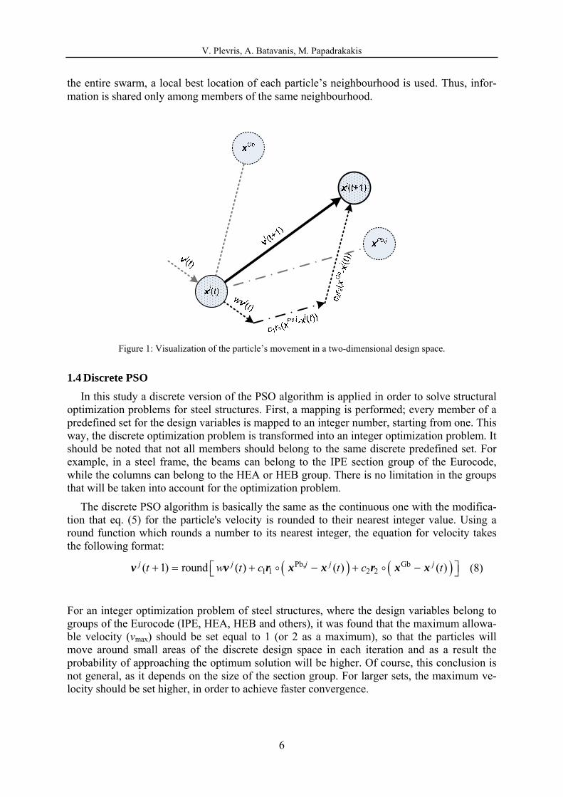
Figure 1 depicts a particle’s movement, in a two-dimensional design space, according to

Eqs. (5) and (6). The particle’s current position xj(t) at time t is represented by the dotted cir-cle at the lower left of the drawing, while the new position xj(t+1) at time t+1 is represented by the dotted bold circle at the upper right-hand corner of the drawing. It can be seen how the particle’s movement is affected by: (i) it’s velocity vj(t); (ii) the personal best ever position of the particle, xPb,j, at the right of the figure; and (iii) the global best location found by the entire swarm, xGb, at the upper left of the figure.

In the above formulation, the global best location found by the entire swarm up to the cur-rent iteration (xGb) is used. This is called a fully connected topology (fully informed PSO), as all particles share information with each other about the best performer of the swarm. Other topologies have also been used in the past where instead of the global best location found by


6

the entire swarm, a local best location of each particle’s neighbourhood is used. Thus, infor-mation is shared only among members of the same neighbourhood.

Figure 1: Visualization of the particle’s movement in a two-dimensional design space.

1.4 Discrete PSO

In this study a discrete version of the PSO algorithm is applied in order to solve structural optimization problems for steel structures. First, a mapping is performed; every member of a predefined set for the design variables is mapped to an integer number, starting from one. This way, the discrete optimization problem is transformed into an integer optimization problem. It should be noted that not all members should belong to the same discrete predefined set. For example, in a steel frame, the beams can belong to the IPE section group of the Eurocode, while the columns can belong to the HEA or HEB group. There is no limitation in the groups that will be taken into account for the optimization problem.

The discrete PSO algorithm is basically the same as the continuous one with the modifica-tion that eq. (5) for the particle's velocity is rounded to their nearest integer value. Using a round function which rounds a number to its nearest integer, the equation for velocity takes the following format:

Pb, Gb1 1 2 2( 1) round ( ) ( ) ( )j j j j jt w t c t c t v v r x x r x x (8)

For an integer optimization problem of steel structures, where the design variables belong to groups of the Eurocode (IPE, HEA, HEB and others), it was found that the maximum allowa-ble velocity (vmax) should be set equal to 1 (or 2 as a maximum), so that the particles will move around small areas of the discrete design space in each iteration and as a result the probability of approaching the optimum solution will be higher. Of course, this conclusion is not general, as it depends on the size of the section group. For larger sets, the maximum ve-locity should be set higher, in order to achieve faster convergence.


7

1.5 Genetic Algorithm

The Genetic Algorithm (GA) method is the most widely used type of Evolutionary Algo-rithm. In a genetic algorithm, a population of strings (called chromosomes or genotype), which encode candidate solutions (called individuals or phenotypes) of the optimization prob-lem, evolves toward better solutions. Traditionally, solutions are represented in binary form as strings of 0s and 1s, but other encodings are also possible. The evolution usually starts from a population of randomly generated individuals and takes place in generations. In each genera-tion, the fitness of every individual in the population is evaluated, multiple individuals are stochastically selected from the current population based on their fitness, and modified to form a new population. The new population is then used in the next iteration of the algorithm and this procedure goes on until the optimum solution is found or a convergence criterion has been satisfied. Commonly, the algorithm terminates when either a maximum number of gen-erations has been reached, or a satisfactory fitness value has been achieved for a member of the population. The GA method consists of the following processes:

a) Encoding of the information carried by the chromosomes using fixed-length binary strings.

b) Fitness evaluation, where the objective function value is calculated. c) Selection of members who will become parents and will produce the next genera-

tion (Tournament selection, Ranking selection, Roulette Wheel). d) Crossover operator (Scattered crossover, One-point crossover, Two-point crossover,

Uniform crossover, Arithmetic crossover, Heuristic crossover). e) Mutation operator, which is an operator that inserts a small probability that a single

binary bit in a given chromosome will be changed from its initial value. The main purpose of the mutation operator is to maintain diversity within the population and inhibit premature convergence.

f) Termination of the algorithm, when convergence has been achieved.

In a structural constrained optimization problem the steps of the Genetic Algorithm are briefly shown in the following figure

1. Initialization: Selection of parent vectors of the design variables, usually randomly. 2. Analysis and Evaluation: Evaluation of the parents by the fitness function. 3. Feasibility Check: If not all parents are feasible, modification of infeasible parents and

back to step 2. 4. Genetic Operators: Mutation of all members and crossover of parents to produce off-

spring. 5. Analysis and Evaluation: Evaluation of the offspring by the fitness function. 6. Feasibility Check: If not all offspring are feasible, discard infeasible offspring and

back to step 4. 7. Genetic Operators: Selection, mutation and crossover of the next generation parents. 8. Termination Criterion: If any one of the termination criteria is reached then stop, else

go back to step 4.

Figure 2: GA steps in constrained optimization problems.


8

1.6 Constraint Handling Technique for PSO

The structural optimization problems are subjected to a number of inequality constraints. These constraints impose limitations to the values that the design variables can take and limit the available search space in which the optimum solution can be searched and found. In gen-eral, different optimization methods handle constraints in different ways. In this study a penal-ty method will be used to handle the constraints of the PSO problem and in particular the penalty method proposed by Plevris [20] which is proven to be a simple and effective method which in the case of a typical constraint has the following form:

,( ) ( ) 0k k allow kg q q x x (9)

where ( )kq x is a response measure (usually displacement, stress or strain) for design vector

x and ,allow kq its maximum allowable absolute value.

In this case the penalty function ( )k x for the typical constraint is the following:

,

, ,

( )1 1

( )( ) ( )

1

k

allow k

k

k k

allow k allow k

qif

q

q qif

q q

x

xx x

(10)

Having calculated the penalty function for all violated constraints, the penalized fitness value of a design x is obtained by multiplying the objective function to be minimized (struc-tural weight) by the maximum penalty factor among all constraints:

( ) ( ) max ( )p kf f x x x (11)

where ( )pf x is the new penalized objective function and max ( )k x the maximum value

of the penalty function among all active constraints of the optimization problem. Using the previous method, there is a case where the penalized objective function can ob-

tain a better value compared to the optimum solution found at the iteration n of the algorithm, GBestn. This undesirable case resets the best solution into the infeasible areas of the design space. To avoid this problem, the penalty is imposed on the optimum solution instead of the new objective function, as shown in the following equations:

( ) ( ) max ( ) max ( ) 1 ( )

( ) max ( ) max ( ) 1 ( )

p k k n

p n k k n

f f x if and f Gbest

f Gbest x if and f Gbest

x x x x

x x x(12)

2 LINEAR STATIC ANALYSIS TOOL

A new software tool for the linear static analysis of three-dimensional frames has been de-veloped, featuring some distinct characteristics. The applied loads can be nodal or elemental (uniform, triangular or trapezoidal in any direction - x, y, z - within an element), while any release (translational or rotational) can be implemented at an end of any element, in any of the 6 Degrees Of Freedom (DOFs), either translational or rotational. The input file of the program contains the information that is shown in Table 1.


9

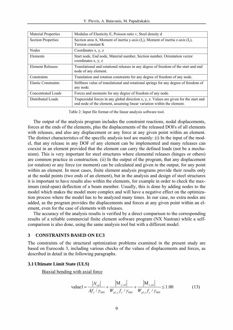
Material Properties Modulus of Elasticity E, Poisson ratio v, Steel density d

Section Properties Section area A, Moment of inertia y-axis (Iy), Moment of inertia z-axis (Iz), Torsion constant K

Nodes Coordinates x, y, z

Elements Start node, End node, Material number, Section number, Orientation vector coordinates x, y, z

Element Releases Translational and rotational releases in any degree of freedom of the start and end node of any element.

Constraints Translation and rotation constraints for any degree of freedom of any node.

Elastic Constraints Stiffness value of translational and rotational springs for any degree of freedom of any node.

Concentrated Loads Forces and moments for any degree of freedom of any node.

Distributed Loads Trapezoidal forces in any global direction x, y, z. Values are given for the start and end node of the element, assuming linear variation within the element.

Table 2: Input file format of the linear analysis software tool.

The output of the analysis program includes the constraint reactions, nodal displacements, forces at the ends of the elements, plus the displacements of the released DOFs of all elements with releases, and also any displacement or any force at any given point within an element. The distinct characteristics of the specific analysis tool are mainly: (i) In the input of the mod-el, that any release in any DOF of any element can be implemented and many releases can coexist in an element provided that the element can carry the defined loads (not be a mecha-nism). This is very important for steel structures where elemental releases (hinges or others) are common practice in construction. (ii) In the output of the program, that any displacement (or rotation) or any force (or moment) can be calculated and given in the output, for any point within an element. In most cases, finite element analysis programs provide their results only at the nodal points (two ends of an element), but in the analysis and design of steel structures it is important to have results also within the elements, for example in order to check the max-imum (mid-span) deflection of a beam member. Usually, this is done by adding nodes to the model which makes the model more complex and will have a negative effect on the optimiza-tion process where the model has to be analyzed many times. In our case, no extra nodes are added, as the program provides the displacements and forces at any given point within an el-ement, even for the case of elements with releases.

The accuracy of the analysis results is verified by a direct comparison to the corresponding results of a reliable commercial finite element software program (NX Nastran) while a self-comparison is also done, using the same analysis tool but with a different model.

3 CONSTRAINTS BASED ON EC3

The constraints of the structural optimization problems examined in the present study are based on Eurocode 3, including various checks of the values of displacements and forces, as described in detail in the following paragraphs.

3.1 Ultimate Limit State (ULS)

Biaxial bending with axial force

, ,

0 , 0 , 0

value1 1.00/ / /

y sd z sdsd

y pl y y pl z y

N

Af W f W f

(13)


10

Shear force (Y-axis)

,

y

, 0

value2 1.003

y sd

y y

V

A f (14)

Shear force (Z-axis)

,

z

, 0

value2 1.003

z sd

z y

V

A f (15)

where:

sdN , ,y sd , ,z sd : Axial force, bending moment around y - axis and bending moment around

z - axis, respectively

,y sdV , ,z sdV : y - shear force and z - shear force, respectively

,pl yW , ,pl zW : Plastic section modulus around y and z - axis, respectively

A : Section area

yf : Yield stress of steel

0 : The partial safety factor ( 0 1.00 according to EC3)

, yA , , zA : Shear area for y - axis and z - axis, respectively

The above ULS constraints are checked for the following load combinations:

a) 1.35G +1.50Q + 0.60W

b) 1.35G +1.50W + 0.60Q

c) 1.00G +0.30Q + E

Where G are the deal loads, Q are the live loads, W are the wind loads and E are the earth-quake loads on the structure which are imposed using the equivalent static method of the Greek Seismic Code (EAK2000), which is similar to the lateral force method of the Eurocode 8.

3.2 Serviceability Limit State (SLS)

Serviceability check for full loading:

250

value3 1.00zv

L (16)

for the following load combinations:


11

a) 1.00G +1.00Q + 0.60W

b) 1.00G +1.00W + 0.70Q

Serviceability check for live loading only (without dead loads):

300

value4 1.00zv

L (17)

for the following load combinations:

a) 1.00Q + 0.60W

b) 1.00W + 0.70Q

where vz is the vertical displacement at the middle of a beam element.

The constraint values are calculated for every element of the steel frame, in various posi-tions within the element (L/10, 2L/10, etc). The objective function of the structural optimiza-tion problem is the weight of the structure, to be minimized, which is described in Eq. (2).

4 NUMERICAL EXAMPLES

4.1 Verification of the linear static analysis tool

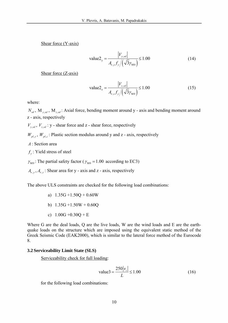
A Finite Element analysis of a three-dimensional frame is performed. The model (A) is de-picted in Figure 3.

Figure 3: Three-dimensional analysis model A for verification purposes.


12

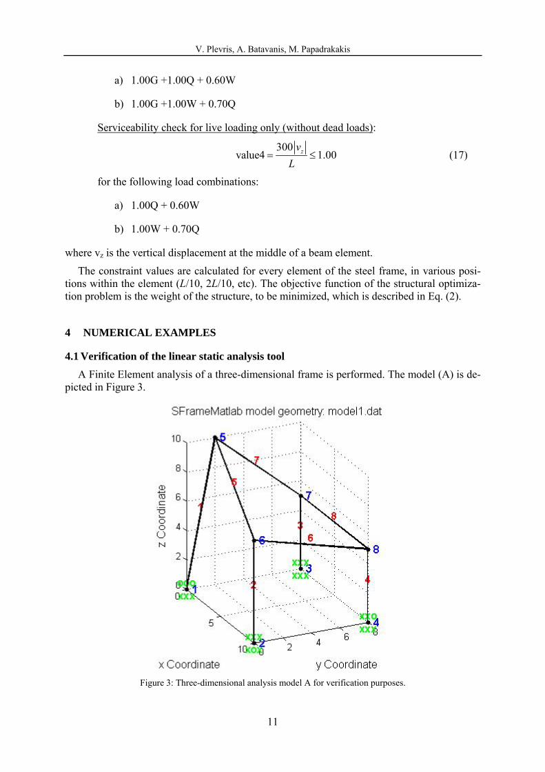
Various types of loads, releases and springs are applied, as shown in the tables below.

Node Node Coordinates (m) Constraints

x y z Translations Rotations Description

1 0 0 0 ΧΧΧ ΟΟΟ Hinge

2 10 0 0 ΧΟΧ ΧΧΧ Y-Translation allowed

3 0 8 0 ΧΧΧ ΧΧΧ Fixed

4 10 8 0 ΧΧΧ ΧΧΟ Z-Rotation allowed

5 0 2 10 - - -

6 10 0 7 - - -

7 0 8 5 - - -

8 10 8 5 - - -

Table 3: Nodal data of the analysis model A (X denotes restriction of the DOF, O denotes free DOF.

Element Start Node End Node Coordinates of Orientation Vector (R)

xR yR zR

1 1 5 0 8 5

2 2 6 10 8 5

3 3 7 0 2 10

4 4 8 10 0 7

5 5 6 0 8 5

6 6 8 0 2 10

7 5 7 10 8 5

8 7 8 10 0 7

Table 4: Elemental data of the analysis model A.

Element Start Node End Node Release Description

Translations Rotations Translations Rotations

4 000 000 100 001 X-translation and Z-

rotation at the end node of the element

5 000 000 001 010 Z-translation and Y-

rotation at the end node of the element

Table 5: Elemental releases of the analysis model A.

Node Degree Of Freedom Stiffness value Description

6 1 5000 Translational Spring (X-

axis)

8 4,5,6 2000 Rotational Springs

(X,Y,Z axes)

Table 6: Spring data of the analysis model A.


13

Node Fx (kN) Fy (kN) Fz (kN) Mx (kNm) My (kNm) Mz (kNm)

5 10 -25 -20 0 25 50

6 10 -20 -10 50 0 0

7 10 -10 10 0 -50 30

8 -20 10 30 0 0 0

Table 7: Nodal loads of the analysis model A (global system).

Element ixF

(kN/m)

jxF

(kN/m)

iyF

(kN/m)

jyF

(kN/m)

izF

(kN/m)

jzF

(kN/m)

5 -20 35 15 -30 0 0

7 10 -10 -25 15 0 0

Table 8: Elemental loads of the analysis model A.

Material properties: 8 22.1 10 kN/m , 0.3E v

Section properties: 3 2 5 4 6 4 7 45 10 m , 8 10 m , 6 10 m , 2 10 my zA I I K

Results The analysis tool calculates the displacements, forces and moments at any given interme-

diate point of any element. Having calculated the displacements at any given point of the ele-ment, the software provides a figure of the deformed shape of the analysis model, which for model A is shown in Figure 4.

Figure 4: Deformed shape of the analysis model A.


14

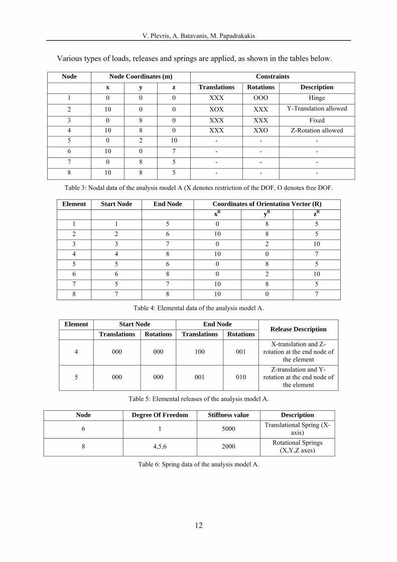
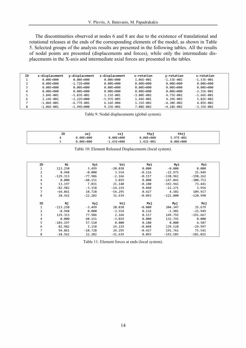
The discontinuities observed at nodes 6 and 8 are due to the existence of translational and rotational releases at the ends of the corresponding elements of the model, as shown in Table 5. Selected groups of the analysis results are presented in the following tables. All the results of nodal points are presented (displacements and forces), while only the intermediate dis-placements in the X-axis and intermediate axial forces are presented in the tables.

ID x‐displacement y‐displacement z‐displacement x‐rotation y‐rotation z‐rotation 1 0.00E+000 0.00E+000 0.00E+000 1.06E‐001 ‐1.33E‐002 ‐1.53E‐001 2 0.00E+000 ‐1.72E+000 0.00E+000 0.00E+000 0.00E+000 0.00E+000 3 0.00E+000 0.00E+000 0.00E+000 0.00E+000 0.00E+000 0.00E+000 4 0.00E+000 0.00E+000 0.00E+000 0.00E+000 0.00E+000 ‐3.35E‐002 5 3.84E‐001 ‐5.83E‐001 1.15E‐001 ‐3.80E‐002 4.75E‐002 ‐1.66E‐001 6 2.14E‐002 ‐2.22E+000 ‐5.97E‐005 1.44E‐001 4.39E‐003 5.02E‐002 7 ‐1.06E‐001 ‐6.77E‐001 6.16E‐004 1.31E‐002 ‐4.30E‐002 4.85E‐002 8 ‐1.06E‐001 ‐1.99E+000 9.33E‐001 7.08E‐002 ‐4.18E‐002 ‐3.35E‐002

Table 9: Nodal displacements (global system).

ID uxj vzj thyj thzj 4 0.00E+000 0.00E+000 0.00E+000 5.97E‐001 5 0.00E+000 ‐1.65E+000 1.42E‐001 0.00E+000

Table 10: Element Released Displacements (local system).

ID Ni Vyi Vzi Mxi Myi Mzi 1 113.250 3.499 ‐20.038 0.000 ‐0.000 0.000 2 8.948 ‐0.000 3.554 ‐0.116 ‐22.975 25.949 3 ‐129.313 ‐77.986 ‐2.166 ‐0.157 ‐138.961 ‐198.262 4 0.000 ‐60.151 3.019 0.000 ‐147.841 ‐300.753 5 13.197 7.031 21.140 ‐0.180 ‐192.942 73.441 6 ‐82.982 ‐3.158 ‐14.219 0.048 ‐22.271 3.956 7 ‐64.861 10.728 ‐54.295 0.427 4.502 109.917 8 18.562 ‐22.202 31.639 ‐0.093 ‐122.800 ‐120.998

ID Nj Vyj Vzj Mxj Myj Mzj 1 ‐113.250 ‐3.499 20.038 ‐0.000 204.347 35.679 2 ‐8.948 0.000 ‐3.554 0.116 ‐1.901 ‐25.949 3 129.313 77.986 2.166 0.157 149.792 ‐191.667 4 0.000 60.151 ‐3.019 0.000 132.745 0.000 5 ‐103.197 57.510 0.000 0.180 0.000 4.507 6 82.982 3.158 14.219 ‐0.048 139.528 ‐29.997 7 94.861 ‐10.728 29.295 ‐0.427 191.761 75.541 8 ‐18.562 22.202 ‐31.639 0.093 ‐193.585 ‐101.025

Table 11: Element forces at ends (local system).


15

ID N(0) N(L/10) N(2L/10) N(3L/10) N(4L/10) N(L/2) 1 113.250 113.250 113.250 113.250 113.250 113.250 2 8.948 8.948 8.948 8.948 8.948 8.948 3 ‐129.313 ‐129.313 ‐129.313 ‐129.313 ‐129.313 ‐129.313 4 0.000 0.000 0.000 0.000 0.000 0.000 5 13.197 ‐6.603 ‐20.003 ‐27.003 ‐27.603 ‐21.803 6 ‐82.982 ‐82.982 ‐82.982 ‐82.982 ‐82.982 ‐82.982 7 ‐64.861 ‐78.661 ‐90.061 ‐99.061 ‐105.661 ‐109.861 8 18.562 18.562 18.562 18.562 18.562 18.562

ID N(6L/10) N(7L/10) N(8L/10) N(9L/10) N(L) 1 113.250 113.250 113.250 113.250 113.250 2 8.948 8.948 8.948 8.948 8.948 3 ‐129.313 ‐129.313 ‐129.313 ‐129.313 ‐129.313 4 0.000 0.000 0.000 0.000 0.000 5 ‐9.603 8.997 33.997 65.397 103.197 6 ‐82.982 ‐82.982 ‐82.982 ‐82.982 ‐82.982 7 ‐111.661 ‐111.061 ‐108.061 ‐102.661 ‐94.861 8 18.562 18.562 18.562 18.562 18.562

Table 12: Axial forces at various positions within the elements (local system).

ID u(0) u(L/10) u(2L/10) u(3L/10) u(4L/10) u(L/2) 1 0.00E+000 1.75E‐002 3.64E‐002 5.77E‐002 8.28E‐002 1.13E‐001 2 0.00E+000 3.23E‐004 1.24E‐003 2.69E‐003 4.59E‐003 6.86E‐003 3 0.00E+000 ‐1.04E‐003 ‐4.16E‐003 ‐9.38E‐003 ‐1.67E‐002 ‐2.62E‐002 4 0.00E+000 ‐1.10E‐003 ‐4.37E‐003 ‐9.80E‐003 ‐1.74E‐002 ‐2.70E‐002 5 3.84E‐001 3.36E‐001 2.85E‐001 2.33E‐001 1.78E‐001 1.20E‐001 6 2.14E‐002 ‐1.86E‐002 ‐5.57E‐002 ‐8.87E‐002 ‐1.16E‐001 ‐1.38E‐001 7 3.84E‐001 4.34E‐001 4.36E‐001 3.99E‐001 3.31E‐001 2.43E‐001 8 ‐1.06E‐001 ‐1.06E‐001 ‐1.06E‐001 ‐1.06E‐001 ‐1.06E‐001 ‐1.06E‐001

Table 13: x-displacements (axial) at various positions within the elements (local system).

Results verification: 1. Comparison with NX Nastran

The results obtained by this new tool (nodal displacements and element forces) are com-

pared to the ones obtained with NX Nastran, a reliable commercial finite element software. The corresponding results of NX Nastran for the analysis model A are given in the tables be-low.

ID. T1 T2 T3 R1 R2 R3 1 G 0. 0. 0. 1.063808E‐1 ‐1.334909E‐2 ‐1.534051E‐1 2 G 0. ‐1.718393E+0 0. 0. 0. 0. 3 G 0. 0. 0. 0. 0. 0. 4 G 0. 0. 0. 0. 0. ‐3.351714E‐2 5 G 3.841538E‐1 ‐5.827316E‐1 1.154246E‐1 ‐3.800689E‐2 4.746852E‐2 ‐1.655687E‐1 6 G 2.141272E‐2 ‐2.222949E+0 ‐5.965523E‐5 1.441588E‐1 4.390469E‐3 5.023001E‐2 7 G ‐1.060799E‐1 ‐6.774387E‐1 6.157757E‐4 1.308552E‐2 ‐4.296919E‐2 4.848347E‐2 8 G ‐1.062567E‐1 ‐1.989106E+0 9.326228E‐1 7.083541E‐2 ‐4.175385E‐2 ‐3.351714E‐2

Table 14: NX Nastran results - Nodal displacements (global system).


16

STAT DIST ‐ BENDING MOMENTS ‐ ‐ WEB SHEARS ‐ AXIAL MOM PLANE 1 MOM PLANE 2 SHR PLANE 1 SHR PLANE 2 FORCE TOT TORQUE

0.000 ‐1.421085E‐14 0. ‐3.498626E+0 2.003789E+1 ‐1.132500E+2 2.886580E‐15 1.000 3.567912E+1 ‐2.043472E+2 ‐3.498626E+0 2.003789E+1 ‐1.132500E+2 2.886580E‐15

0.000 ‐2.594859E+1 ‐2.297478E+1 0. ‐3.553616E+0 ‐8.948283E+0 1.159154E‐1 1.000 ‐2.594859E+1 1.900531E+0 0. ‐3.553616E+0 ‐8.948283E+0 1.159154E‐1

0.000 1.982624E+2 ‐1.389613E+2 7.798593E+1 2.166048E+0 1.293129E+2 1.566389E‐1 1.000 ‐1.916673E+2 ‐1.497916E+2 7.798593E+1 2.166048E+0 1.293129E+2 1.566389E‐1

0.000 3.007529E+2 ‐1.478412E+2 6.015058E+1 ‐3.019295E+0 0. 0. 1.000 0. ‐1.327447E+2 6.015058E+1 ‐3.019295E+0 0. 0.

0.000 ‐7.344055E+1 ‐1.929415E+2 ‐7.031394E+0 ‐2.113989E+1 ‐1.319692E+1 1.801822E‐1 1.000 4.507202E+0 0. 5.751010E+1 0. ‐1.031969E+2 1.801822E‐1

0.000 ‐3.955989E+0 ‐2.227148E+1 3.157955E+0 1.421944E+1 8.298228E+1 ‐4.790572E‐2 1.000 ‐2.999715E+1 ‐1.395280E+2 3.157955E+0 1.421944E+1 8.298228E+1 ‐4.790572E‐2

0.000 ‐1.099169E+2 4.501728E+0 ‐1.072832E+1 5.429548E+1 6.486137E+1 ‐4.271201E‐1 1.000 7.554063E+1 ‐1.917606E+2 ‐1.072832E+1 2.929548E+1 9.486137E+1 ‐4.271201E‐1

0.000 1.209979E+2 ‐1.227998E+2 2.220228E+1 ‐3.163852E+1 ‐1.856227E+1 9.328829E‐2 1.000 ‐1.010250E+2 1.935853E+2 2.220228E+1 ‐3.163852E+1 ‐1.856227E+1 9.328829E‐2

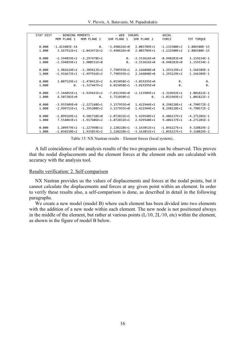
Table 15: NX Nastran results – Element forces (local system)..

A full coincidence of the analysis results of the two programs can be observed. This proves that the nodal displacements and the element forces at the element ends are calculated with accuracy with the analysis tool. Results verification: 2. Self-comparison

NX Nastran provides us the values of displacements and forces at the nodal points, but it cannot calculate the displacements and forces at any given point within an element. In order to verify these results also, a self-comparison is done, as described in detail in the following paragraphs.

We create a new model (model B) where each element has been divided into two elements with the addition of a new node within each element. The new node is not positioned always in the middle of the element, but rather at various points (L/10, 2L/10, etc) within the element, as shown in the figure of model B below.


17

Figure 5: Analysis model B with the addition of new intermediate nodes.

By adjusting the loads, releases, etc, model B has been made equivalent to the first model A. By performing the new analysis, the corresponding results at the nodal points are found to coincide. Also, the intermediate results of the model A at various positions within the ele-ments can now be checked, as in model B there are nodes at these points. By performing the analysis, and doing the corresponding comparisons, it is proven that the results coincide again, as the displacements and forces at the intermediate points within each element are the same as the nodal results of the corresponding new nodes of model B.

4.2 Structural Optimization Problems

One plane and one space steel frame are examined. The optimization results of the discrete PSO method are compared to the ones obtained with a discrete GA. In the discrete structural optimization problems that are examined, three steel section groups have been taken into ac-count, namely the IPE, HEA, HEB section groups of the Eurocode, while it is easy to add other section groups also. In all test examples, the earthquake loading has been taken into ac-count with the equivalent static load method of the Greek Seismic Code (EAK2000), where a peak ground acceleration of 0.36g has been taken into consideration.

The parameters of the GA and PSO algorithms, used in this study, are presented in the fol-lowing tables.

Population size 20

Generations 100

Crossover function Scattered

Table 16: GA parameter values.


18

Swarm size 20

Iterations 100

maxv 1

maxw 0.95

minw 0.8

1 2,c c 2

Table 17: PSO parameter values.

Optimization example 1

The first optimization test example is a plane frame that is depicted in Figure 6. The details of the model are given in the tables below.

Element Dead distributed loads

(kN/m) Live distributed loads

(kN/m) Wind distributed loads

(kN/m)

izG j

zG izQ j

zQ ixW j

xW

1-5 - - - - 3 3

21-35 -2 -2 -0.5 -0.5 - -

Table 18: Load types and values of model 1.

Design variable Elements Section category

1 Beams

21-22, 26-27, 31-32 IPE

2 Beams

23-25, 28-30, 33-35 IPE

3 Columns

1-2, 6-7, 11-12, 16-17 HEA

4 Columns

3-5, 8-10, 13-15, 18-20 HEB

Table 19: Design variables of model 1.


19

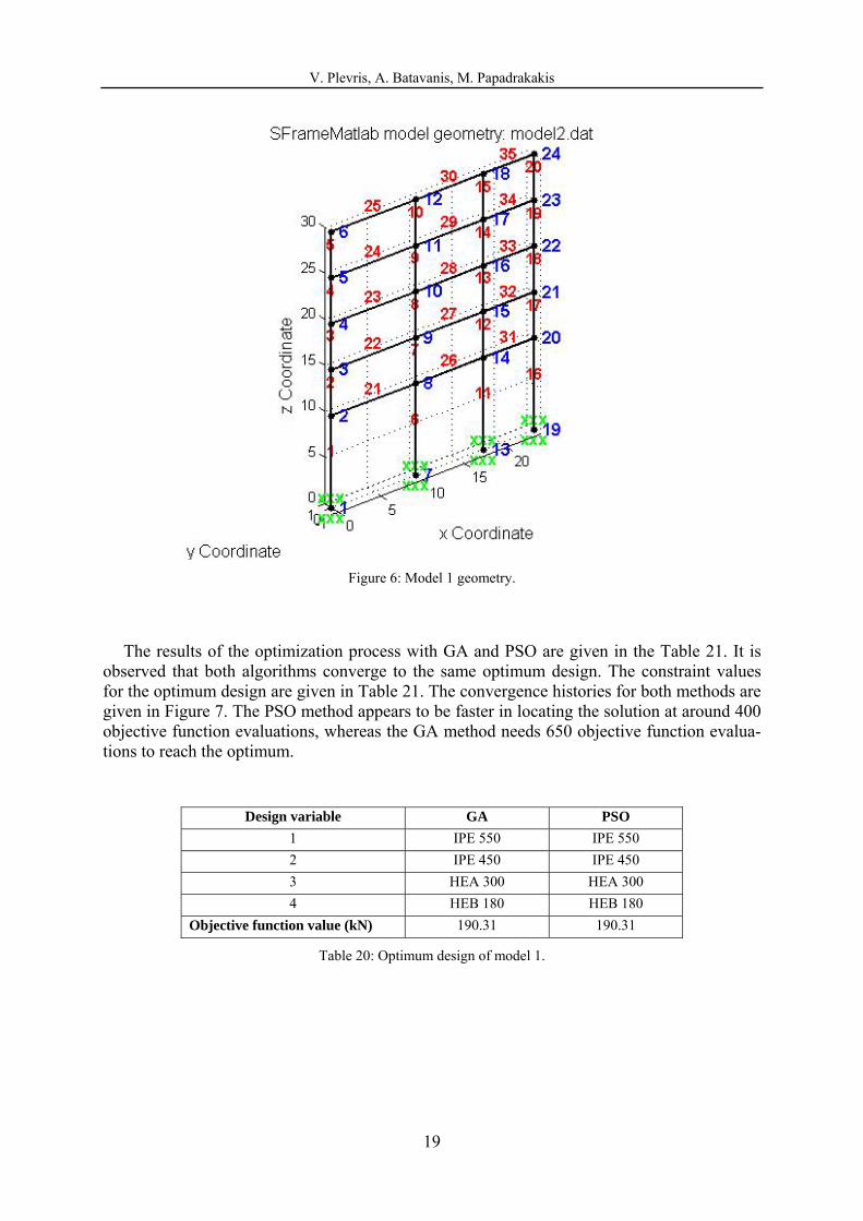
Figure 6: Model 1 geometry.

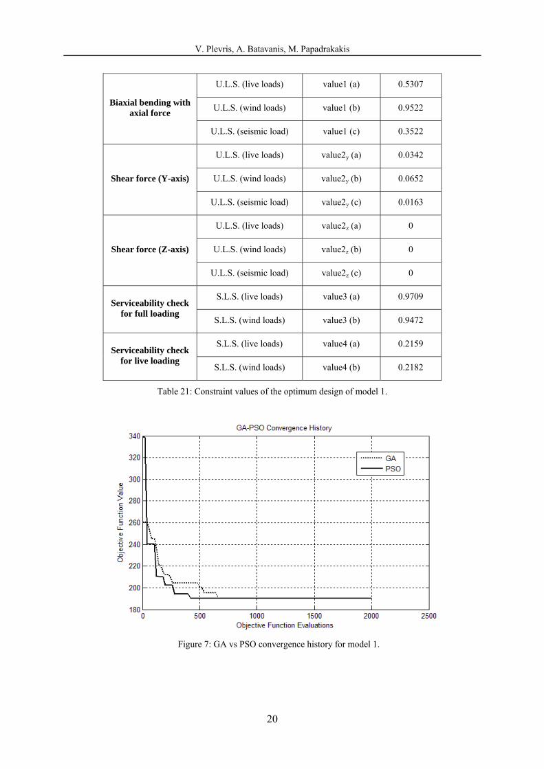
The results of the optimization process with GA and PSO are given in the Table 21. It is observed that both algorithms converge to the same optimum design. The constraint values for the optimum design are given in Table 21. The convergence histories for both methods are given in Figure 7. The PSO method appears to be faster in locating the solution at around 400 objective function evaluations, whereas the GA method needs 650 objective function evalua-tions to reach the optimum.

Design variable GA PSO

1 IPE 550 IPE 550

2 IPE 450 IPE 450

3 HEA 300 HEA 300

4 HEB 180 HEB 180

Objective function value (kN) 190.31 190.31

Table 20: Optimum design of model 1.


20


U.L.S. (live loads) value1 (a) 0.5307

U.L.S. (wind loads) value1 (b) 0.9522

U.L.S. (seismic load) value1 (c) 0.3522


U.L.S. (live loads) value2y (a) 0.0342

U.L.S. (wind loads) value2y (b) 0.0652

U.L.S. (seismic load) value2y (c) 0.0163


U.L.S. (live loads) value2z (a) 0

U.L.S. (wind loads) value2z (b) 0

U.L.S. (seismic load) value2z (c) 0

Serviceability check for full loading

S.L.S. (live loads) value3 (a) 0.9709

S.L.S. (wind loads) value3 (b) 0.9472

Serviceability check for live loading



Table 21: Constraint values of the optimum design of model 1.

Figure 7: GA vs PSO convergence history for model 1.


21

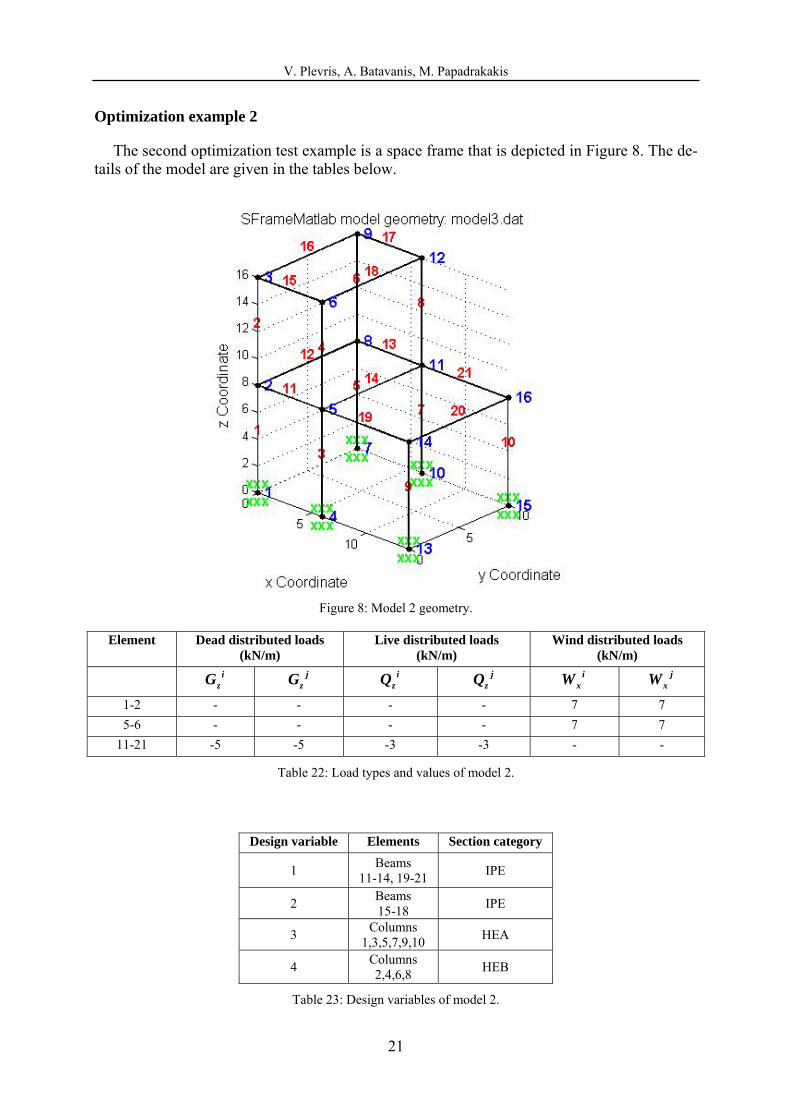
Optimization example 2

The second optimization test example is a space frame that is depicted in Figure 8. The de-tails of the model are given in the tables below.

Figure 8: Model 2 geometry.

Element Dead distributed loads (kN/m)

Live distributed loads (kN/m)

Wind distributed loads (kN/m)

izG j

zG izQ j

zQ ixW j

xW

1-2 - - - - 7 7

5-6 - - - - 7 7

11-21 -5 -5 -3 -3 - -

Table 22: Load types and values of model 2.

Design variable Elements Section category

1 Beams

11-14, 19-21 IPE

2 Beams 15-18

IPE

3 Columns

1,3,5,7,9,10 HEA

4 Columns 2,4,6,8

HEB

Table 23: Design variables of model 2.


22

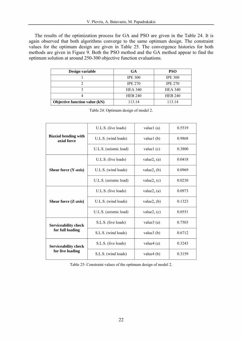
The results of the optimization process for GA and PSO are given in the Table 24. It is again observed that both algorithms converge to the same optimum design. The constraint values for the optimum design are given in Table 25. The convergence histories for both methods are given in Figure 9. Both the PSO method and the GA method appear to find the optimum solution at around 250-300 objective function evaluations.

Design variable GA PSO

1 IPE 300 IPE 300

2 IPE 270 IPE 270

3 HEA 340 HEA 340

4 HEB 240 HEB 240

Objective function value (kN) 113.14 113.14

Table 24: Optimum design of model 2.


U.L.S. (live loads) value1 (a) 0.5519

U.L.S. (wind loads) value1 (b) 0.9868

U.L.S. (seismic load) value1 (c) 0.3800


U.L.S. (live loads) value2y (a) 0.0418

U.L.S. (wind loads) value2y (b) 0.0969

U.L.S. (seismic load) value2y (c) 0.0230


U.L.S. (live loads) value2z (a) 0.0973

U.L.S. (wind loads) value2z (b) 0.1323

U.L.S. (seismic load) value2z (c) 0.0551

Serviceability check for full loading



Serviceability check for live loading



Table 25: Constraint values of the optimum design of model 2.


23

Figure 9: GA vs PSO convergence history of model 2.

5 CONCLUSIONS

The linear static analysis tool that has been developed proved to be a very useful and accu-rate tool for the analysis of three-dimensional frames. The advantage of the software tool is its generality, as it can handle nodal or elemental loads (uniform, triangular or trapezoidal in any direction within an element), any release (translational or rotational) can be implemented at an end of any element, in any of the 6 Degrees Of Freedom (DOFs), while the output of the analysis program includes the displacements of the released DOFs of all elements with releas-es, and any displacement or any force at any given point within an element. The accuracy of the analysis results is verified by a direct comparison to the corresponding results of a reliable commercial finite element software program as well as by performing a self-comparison using an enhanced model with additional nodes.

Both PSO and GA methods proved to be accurate in finding the optimum design almost every single time. GA has a larger computational cost than PSO which exhibited in general better performance in terms of convergence speed. This fact is due to the more complex and time consuming procedures of GA as part of the genetic operators of the algorithm (selection, crossover, mutation). Also the quantity of random numbers generated for each iteration of the algorithm is larger in GA, which makes it slower for a single iteration.

The accuracy of the discrete version of PSO used in this study was quite satisfactory, alt-hough in a small percentage of the tests that were performed, the algorithm was trapped in local optima. Further investigation may be needed for the fine-tuning of the discrete PSO pa-rameters for the optimization problem at hand.

The constraints used in the present study were based on Eurocode 3, but in fact not all Eu-rocode 3 constraints for steel structures have been implemented in the test examples. Most importantly, additional buckling constraints need to be taken into account, as they are many times critical in real world steel structures design. The implementation of these constraints is straight forward given the analysis and optimization frameworks that have been developed, and will be a subject for future research.


24

REFERENCES

[1] Makris, P.A., C.G. Provatidis, and D.A. Rellakis, Discrete variable optimization of frames using a strain energy criterion. Structural and Multidisciplinary Optimization, 2006. 31(5): p. 410-417.

[2] Bremicker, M., P.Y. Papalambros, and H.T. Loh, Solution of mixed-discrete structural optimization problems with a new sequential linearization algorithm. Computers and Structures, 1990. 37(4): p. 451-461.

[3] Hager, K. and R. Balling, New approach for discrete structural optimization. Journal of Structural Engineering (ASCE), 1988. 114(5): p. 1120 - 1133.

[4] Cai, J. and G. Thierauf, Discrete structural optimization using evolution strategies, in Neural Networks & Combinatorial Optimization in Civil & Structural Engineering, B.H.V. Topping and A.I. Khan, Editors. 1993, Civil-Comp Press: Edinburgh.

[5] Cai, J. and G. Thierauf, Discrete optimization of structures using an improved penalty function method. Engineering Optimization, 1993. 21(4): p. 293-306.

[6] Fu, J.-F., R.G. Fenton, and W.L. Cleghorn, A mixed integer-discrete-continuous programming method and its application to engineering design optimization. Engineering Optimization, 1991. 17: p. 263-280.

[7] Kennedy, J. and R. Eberhart, Particle swarm optimization, in IEEE International Conference on Neural Networks. 1995: Piscataway, NJ, USA. p. 1942–1948.

[8] Bochenek, B. and P. Foryś, Structural optimization for post-buckling behavior using particle swarms. Structural and Multidisciplinary Optimization, 2006. 32(6): p. 521-531.

[9] He, Q. and L. Wang, An effective co-evolutionary particle swarm optimization for constrained engineering design problems. Engineering Applications of Artificial Intelligence, 2007. 20(1): p. 89-99.

[10] Liang, J.J. and P.N. Suganthan, Dynamic Multi-Swarm Particle Swarm Optimizer with a Novel Constraint-Handling Mechanism, in Evolutionary Computation, 2006. CEC 2006. IEEE Congress on. 2006. p. 9-16.

[11] Mezura-Montes, E. and B.C. Lopez-Ramirez, Comparing bio-inspired algorithms in constrained optimization problems, in Evolutionary Computation, 2007. CEC 2007. IEEE Congress on. 2007. p. 662-669.

[12] Munoz-Zavala, A.E., et al., PESO+ for Constrained Optimization, in Evolutionary Computation, 2006. CEC 2006. IEEE Congress on. 2006. p. 231-238.

[13] Perez, R.E. and K. Behdinan, Particle Swarm Optimization in Structural Design, in Swarm Intelligence: Focus on Ant and Particle Swarm Optimization, F.T.S. Chan and M.K. Tiwari, Editors. 2007, Itech Education and Publishing: Vienna, Austria. p. 373-394.

[14] Ye, D., Z. Chen, and J. Liao, A New Algorithm for Minimum Attribute Reduction Based on Binary Particle Swarm Optimization with Vaccination, in Advances in Knowledge Discovery and Data Mining. 2007. p. 1029-1036.

[15] Fourie, P.C. and A. Groenwold, The particle swarm optimization algorithm in size and shape optimization. Structural and Multidisciplinary Optimization, 2002. 23(4): p. 259–267.

[16] Venter, G. and J. Sobieszczanski-Sobieski, Multidisciplinary optimization of a transport aircraft wing using particle swarm optimization. Structural and Multidisciplinary Optimization, 2004. 26: p. 121-131.


25

[17] Fourie, P. and A. Groenwold, The particle swarm optimization in topology optimization, in Fourth world congress of structural and multidisciplinary optimization. 2001: Dalian, China.

[18] Perez, R.E. and K. Behdinan, Particle swarm approach for structural design optimization. Computers and Structures, 2007. 85: p. 1579-1588.

[19] Li, L.J., et al., A heuristic particle swarm optimizer for optimization of pin connected structures. Computers and Structures, 2007. 85: p. 340-349.

[20] Plevris, V., Innovative Computational Techniques for the Optimum Structural Design Considering Uncertainties, in School of Civil Engineering. 2009, National Technical University of Athens (NTUA): Athens.

optimum design of steel structures with the...

Documents