comparative assessment on modeling...

COMPDYN 2011

3rd ECCOMAS Thematic Conference on

Computational Methods in Structural Dynamics and Earthquake Engineering M. Papadrakakis, M. Fragiadakis, V. Plevris (eds.)

Corfu, Greece, 25–28 May 2011

COMPARATIVE ASSESSMENT ON MODELING APPROACHES FOR

THE SEISMIC RESPONSE OF RC SHEAR WALLS

C. Stathi1*

, M. Fragiadakis2, A. Papachristidis

1 and M. Papadrakakis

1

1 Department of Civil Engineering, NTUA, Iroon Polytechneiou 9, 15780, Zografou, Athens, Greece

e-mail: {cstathi, aristidi, mpapadra}@central.ntua.gr

2 Department of Civil and Environmental Engineering, University of Cyprus, P.O. Box 20537, 1678

Nicosia, Cyprus

[email protected]

Keywords: Shear Walls, Shear Deformations, Fiber Elements, RC Structures, Slender Walls.

Abstract. Shear deformations may considerably affect the capacity and the failure mode of

reinforced concrete members. Simplified beam-column models typically are not able to cap-

ture this effect and usually are suitable only for members that exhibit a flexure-dominated re-

sponse. Modeling approaches of increasing complexity for the simulation of reinforced

concrete shear walls are compared in this work. More specifically, we compare the common

fiber beam element, a simplified fiber beam element based on the Timoshenko theory that

considers separately shear and bending deformations and a third Timoshenko beam element

where a multidimensional concrete law is used. The various approaches are discussed and

compared against experimental results. It is worth noting that experiments implemented for

the comparison exhibit different failure modes, flexural as well as shear failure. The numeri-

cal study provides an insight to the efficiency of the above methods in terms of computing de-

mand, accuracy and ease of implementation.

C. Stathi, M. Fragiadakis, A. Papachristidis and M. Papadrakakis

2

1 INTRODUCTION

Recent earthquakes have demonstrated that often reinforced concrete (RC) members fail

under shear. Moreover, shear walls increase the stiffness and the deformation capacity of RC

structures when subjected to inelastic cyclic deformations such as those imposed by strong

seismic ground motions. Therefore, proper modeling of members of the effect of shear is es-

sential for the seismic capacity assessment of RC structures.

Four alternative modeling approaches for the simulation of reinforced concrete frame

members are here compared. The first approach is the common fiber-based beam element

where shear effects are neglected. The second approach is also a fiber beam-column formula-

tion, based on the Timoshenko theory. This element uses the fiber approach to capture bend-

ing and a separate shear force-shear strain relationship (V-γ) to capture the shear in the section

level. Since separate laws are used for the fibers and the shear effect, this approach is called

the “decoupled approach” [1, 2]. A more elaborate approach, also based on a Timoshenko fi-

ber beam-column formulation, is adopted. In the latter case, a three-dimensional constitutive

law for the concrete fibers is used, thus offering a full coupling between bending and shear

strains [2, 3]. Our study includes also the Multiple-Vertical-Line-Element Model (MVLEM)

approach as discussed by Massone and Wallace [4]. MVLEM is a macro-model element, able

to incorporate important response parameters such as confinement, nonlinear shear behavior

and migration of the neutral axis.

After a brief presentation of the models adopted, a comparative assessment on RC mem-

bers subjected to different loading is presented. To evaluate the effectiveness and the reliabil-

ity of the modeling approaches, our results are compared with available experimental data.

2 FINITE ELEMENT FORMULATIONS

The beam-column formulations implemented follow the force-based formulation, also

known as flexibility formulation [5] for fiber-based, beam-column elements. Compared to

displacement-based elements, this approach improves considerably the accuracy and the effi-

ciency of the analysis [2, 3]. According to the force-based approach, the element flexibility

matrix is calculated after integrating the section stiffnesses ksec, as:

1

1T

N sec

1

d

F b k b (1)

where FN is the element flexibility matrix and b(ξ) is the force shape function matrix which

calculates the section forces from the element forces. The element natural stiffness matrix is

therefore calculated as:

1

N N

K F (2)

The element Cartesian stiffness is obtained from the expression:

N N N

TK a K a (3)

where aN contains algebraic calculations and relates the displacements in the local cartesian

and the natural system. The section stiffness matrix ksec of Equation (1) is obtained as the par-

tial derivative of the section forces Dsec over the section deformations dsec, and is calculated as

[2,3]:

T

sec S s

A

dA k a Ca (4)

where C is the material constitutive matrix and as is the section strain distribution matrix.


3

sec

( ) ( ) ( ), , ,s

y z y zε a d (5)

More details about the fiber element formulation and the notation used above can be found in

[2, 3].

2.1 Fiber element based on Euler-Bernoulli beam theory

The simplest force-based fiber element formulation (Bernoulli EB) is based on the Euler-

Bernoulli assumption and therefore shear deformations are neglected. In this case, the section

stiffness will be:

2

, ,

1 2

i i i i i i i infib

T

s EB s EB i i i i i i i i i isec

iA

i i i i i i i i i i

=

E A y E A z E A

dA y E A y E A y z E A

z E A y z E A z E A

a Cak (6)

where C is a scalar and equal to the tangent Young modulus Ei of the ith

fiber, Ai is the area of

the fiber, and yi, zi denote the coordinates of the fibers with respect to the centroid of the

cross-section.

In Eq. (6) as,EB is the section strain distribution matrix of Eq. (5) which here takes the

form:

,( , ) 1

s EBy z y z a . (7)

2.2 Decoupled fiber element

This model consists of a shear spring connected in series with a beam-column element.

This idea was initially presented by Marini and Spacone [1]. In order to take into considera-

tion shear strains, a phenomenological V-γ shear law is implemented at the section level, and

therefore the shear strains are uncoupled from axial and bending strains. This is a simplifying

assumption that maintains all the advantages of fiber elements in terms of robustness and

simplicity of the material laws adopted. The section stiffness will be:

sec

0 0

/ 0

0 /

EB

sec y xy

z xz

dV d

dV d

k

k 0

0

. (8)

where sec

EBk is the stiffness matrix of Eq. (6) and dV/dγ is the slope of the V-γ relationship.

Α bilinear or a trilinear V-γ relationship can be used as discussed in a following section.

In the linear elastic range dV/dγ is equal to the product of the shear modulus times the area of

the section (GA). It is noted that since this approach (Decoupled TB) is based on the Timo-

shenko assumption, the elastic stiffness of the element is different than that of the Euler-

Bernoulli case.

2.3 Shear-Deformable fiber element

Compared to the previous two elements this is a more elaborate formulation that considers

the axial-moment-shear interaction. In this case the material matrix C has dimensions 3×3 and

is given by the expression:

11 12 13

21 22 23

31 32 33

y

z

C C C

C q C C

C C q C

C =

σ

ε. (9)


4

In Eq. (9) in order to take into consideration that the shear stresses are not constant

throughout the section, as Timoshenko beam theory assumes, the scaled shear stress distribu-

tion factors qy, qz are introduced. Moreover, the section strain distribution matrix of Eq. (5)

takes the form:

,

( )

1 0 0 0 0

0 0 0 1 0 1 0

0 10 0 0 0 1

s EB

s

y z

y, z

a

a 0

0

. (10)

Eq. (10) leads to the section stiffness matrix:

11 , , 21 , 31 ,

21 , 22 23

1

31 , 32 33

i T i i

s EB s EB s EB s EBnfib

T i T i i

s s s EB ysec

i i T i iA

s EB z

C C C

dA C q C C

C C q C

a a a a

a Ca ak

a

. (11)

where y and z are the coordinates of an arbitrary point in the section.

Complicated materials are often described in the 3D continuum, thus hampering their ap-

plication to structural elements such as beams, plates or shells. In order to incorporate a 3D

material law we impose a condition of transverse equilibrium at every monitoring section [6].

, , , , , ,

0 0y c y c y s y s y c y s

A A

. (12)

where σy,c and σy,s are the stresses developed in the concrete and the stirrups respectively, Ay,c

and Ay,s are the area of concrete and the stirrups, respectively, in the monitoring vertical sec-

tion and ρν is the shear reinforcement ratio.

2.4 The Multiple-Vertical-Line-Element Model approach

The generic Multi-Vertical-Line-Element model (Figure 1) consists of a series of truss el-

ements (or macro-fibers) connected to infinitely rigid beams at their top and bottom. The

number of truss elements can be increased to obtain a more refined description of the wall

cross section. The shear response of the wall element is simulated with a horizontal spring, as

originally suggested by Vulcano et al. [7].

The relative rotation between the top and bottom end of the wall element occurs around a

point placed on the central axis of the element at height hc=c×h, where h is the height of the

shear wall. A suitable value of parameter c is based on the expected curvature distribution

along the element height. Although an accurate assessment of c is not necessary, if we use a

moderate number of MVLEM elements within the yielding region are used, a value of c=0.4

is recommended based on experimental results [8, 9].


5

Figure 1: Schematic representation of the MVLEM.

The shear wall is modeled as a stack of m elements, placed one upon the other [4, 8]. A

single two-dimensional MVLEM has 6 degrees of freedom, located at the center of the rigid

beams of its top and its bottom cross-sections (Figure 1). In order to calculate the strains of

the truss elements, it is assumed that the top and bottom sections remain plane. The stiffness

matrix of an MVLEM element, will be:

T

eK e Ke . (13)

where e is a transformation matrix used to extract the extension and the relative rotations at

the two ends from the element Cartesian degrees of freedom (Figure 1). The transformation

matrix e is given by the formula:

0 1 0 0 1 1

1 / 0 1 1 / 0 0

1 / 0 0 1 / 0 1

h h

h h

e (14)

and the element stiffness matrix Ke of Eq. 14 will be:

1 1 1

2 2 2 2 2

1 1 1

22 2 2 2

1 1 1

1

1 1

n n n

i i i i i

i i i

n n n

i i H i i H i i

i i i

n n n

i i H i i H i i

i i i

k k x k x

k x k c h k x k c c h k x

k x k c c h k x k c h k x

K =

(15)

where kH is the stiffness of the horizontal spring, ki is the stiffness of the ith

truss element and

xi is the distance of the ith

truss element to the central axis of the MVLEM element.

3 MATERIAL MODELS

The uniaxial stress-strain relationship used for the concrete fibers follows the modified

Kent and Park model [10]. In the coupled shear-deformable fiber element where a 3D material


6

law is necessary, the same relationship for each of the principal axes is adopted, while in or-

der to take fracture into consideration, a three-dimensional rotating crack model is employed

[2, 3]. Although this is not strictly a multidimensional concrete law, this approach is able to

yield robust results of increased accuracy. The hysteretic response of reinforcing steel follows

according to the stress–strain relationship proposed by Menegotto and Pinto [11], as extended

by Filippou et al. [12] to include isotropic strain hardening.

When a shear V-γ law is used for the decoupled–shear deformable beam element, a bilinear

curve is defined. Two different approaches for calculating the V-γ law were examined. The

first approach is based on the shear law proposed by Gerin and Adebar [13] and the second

approach is discussed in Mergos and Kappos [14]. The two different V-γ curves are shown in

Figure 2.

Figure 2: Shear force versus shear strain (V-γ) relationship used for the shear component is obtained as discussed

in [13] and [14].

According to the first approach [13], the envelope is primarily defined by the shear stress

and strain at yield, which are used to estimate the ultimate shear strain. The first branch con-

nects the origin with the peak point (VRd, γy). The section shear capacity VRd was calculated

according to Eurocode 2 (2004) [15], while the shear strain at yield is given by the following

equation:

4y y y

ys v s c

f v n vγ

E ρ E E

(16)

where fy is the reinforcement yield stress, Es is the reinforcement modulus of elasticity, vy is

the applied shear stress(at yield), n is the vertical axial compression, ρv is the vertical rein-

forcement ratio and Ec is the tangent stiffness of the concrete. The ultimate shear strain γu is

obtained using the shear strain at yield from the following relationship for the shear strain

ductility μγ:

4 12u

c

vγμ

fγ

y

y

(17)

Here perfect plasticity is assumed, so the section shear capacity at ultimate strain coincides

with that of the shear strain at yield (VRd=Vu).


7

According to the second approach discussed in [14], the bilinear curve is defined by a

cracking point and the failure point. The shear force at cracking is given by the relationship of

Sezen and Moehle [16]:

1/

0.80ctm

cr g

s ctm g

f NV A

L h f A

(18)

where fctm is the mean concrete tensile strength, N is the compressive axial load, Ls/h is the

shear span ratio, and Ag is the gross area of the concrete section. Assuming a parabolic shear

strength distribution along the cross section, the initial shear stiffness GAeff is calculated as

GAeff = G∙(0.80Ag) where G is the elastic shear modulus. The second and third branches share

the same slope, connecting the cracking point to the failure point, and separated at the flexural

yielding point (Vy,γy). The mean shear strain γu is estimated using the truss analogy [17, 18]:

,

2 3

1

' cot sin cos cot

Rd scr

ueff

cs sw

VV sγ

G Ad d E A E b

(19)

where Asw is the area of the transverse reinforcement oriented parallel to the shear force, d-d’

is the distance between the centers of the longitudinal reinforcement, s the spacing of trans-

verse reinforcement, b is the width of the cross-section, Ec is the elastic modulus of concrete,

Es the elastic modulus of steel, θ is the angle defined by column axis and the direction of the

diagonal compression struts and VRd,s is the shear strength contributed by the transverse rein-

forcement [15].

4 NUMERICAL EXAMPLES

A numerical investigation has been carried out using two RC shear walls and an RC col-

umn specimen. The two shear walls (denoted as SW30 and SW33) were tested under mono-

tonic and cyclic loading by Lefas and Kotsovos [19], while the RC column was subjected to

cyclic loading by Xiao et al. [20].

The dimensions and the arrangement of the reinforcement of the wall specimens are shown

in Figure 3. They are 0.65m wide, 1.3m high and their thickness is 0.065m. Both walls were

monolithically connected to a beam in their base. The vertical and the horizontal reinforce-

ment comprises of high-tensile deformed steel bars of 8mm and 6.25mm diameter, respective-

ly. Additional reinforcement in the form of stirrups confine the wall edges using mild steel

bars of 4mm diameter. The properties of the reinforcing bars are shown in Table 1. The cube

strength fcu at the day of testing was 30.1 MPa for the SW30 and 49.2 MPa for the SW33

shear wall.


8

Diameter(mm) syf (MPa)

suf (MPa)

8 470 565

6.25 520 610

4 420 490

Table 1: Properties of the reinforcing bars.

Figure 3: Geometry and reinforcement of the shear

wall specimens.

The SW30 wall was modeled using the Bernoulli EB, Decoupled TB and Shear-

deformable TB simulation with a single force-based element. For all elements five Gauss-

Lobatto integration points were used. For the MVLEM approach, one macroelement has been

adopted. The analysis results of all models are compared to experimental results and are

summarized in Figure 4. Considerable differences between numerical and experimental re-

sults for both stiffness and ultimate strength are observed for the Bernoulli EB model. The

Decoupled TB model curve gives improved results but still is not able to closely predict the

experimental results. The curve obtained by the shear-deformable fiber element exhibits good

accuracy compared to the experimental curve. Implementing the MVLEM approach, the dis-

crepancy for the ultimate strength is reduced, but the stiffness is overestimated for displace-

ments between 5 and 10 mm.

Figure 4: Experimental and numerical results for specimen SW30.


9

The sensitivity of the numerical results to the shear law assigned to the shear spring for the

Decoupled TB element is shown in Figure 5. The results correspond to the to the two different

envelope curves of Figure 2 and are compared with experimental results and those of the

common fiber element (Bernoulli EB). It can be observed that numerical models overestimate

the initial stiffness and the ultimate strength of the wall compared to the experimental results.

However, they give a more representative response compared to Bernoulli EB model, since

shear deformations have been taken into consideration, even though the model neglects the

interaction between moment and shear.

Figure 5: Influence of the shear – law used for the decoupled shear–deformable element on SW30 shear wall.

Figure 6: Influence of the number of MVLEM elements used for the uncoupled shear–deformable element on

SW30 shear wall.

A parametric study on the sensitivity on the number of MVLEM elements is shown in Fig-

ure 6. The initial stiffness is correctly calculated regardless of the number of MVLEM ele-

ments. Contrary to the initial stiffness, the ultimate strength is affected by the number of

elements. When one MVLEM element is implemented, the ultimate strength is overestimated,

while increasing the number of elements leads to underestimating it. The more elements are

implemented for the analysis, the underestimation is increased and converges to the curve of


10

the 100 elements. It is worth noting that analyses with 20, 27, 42 MVLEM elements was con-

ducted and the results were similar to those of the 100 elements.

The second shear wall specimen (SW33) is similar to the first but is subjected to cyclic in-

stead of monotonic loading. The history of the displacement which was forced at the top of

the wall is shown in Figure 7.

Figure 7: The displacement history adopted of the cyclic tests.

Figure 8: Experimental and numerical results for specimen SW33 of the Bernoulli EB model.

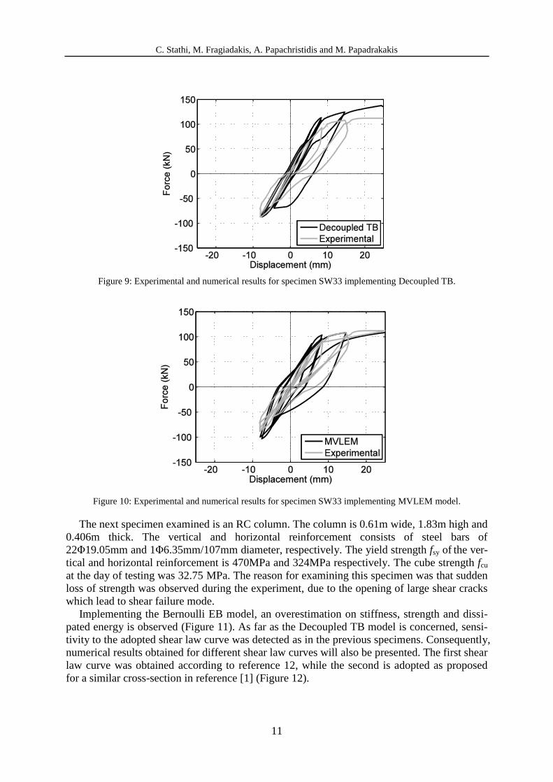
According to Figure 8, the Bernoulli EB model overestimates both stiffness and ultimate

strength. When the Decoupled TB (Figure 9) is implemented, a clear improvement on the

stiffness prediction can be observed. However, again the ultimate strength is overestimated.

Good agreement with experimental results in the prediction of the wall flexural behavior has

been obtained with the MVLEM (Figure 10). The difference on the ultimate strength has been

reduced, while the stiffness is predicted sufficiently in comparison with the Bernoulli EB and

the Decoupled TB models.


11

Figure 9: Experimental and numerical results for specimen SW33 implementing Decoupled TB.

Figure 10: Experimental and numerical results for specimen SW33 implementing MVLEM model.

The next specimen examined is an RC column. The column is 0.61m wide, 1.83m high and

0.406m thick. The vertical and horizontal reinforcement consists of steel bars of

22Φ19.05mm and 1Φ6.35mm/107mm diameter, respectively. The yield strength fsy of the ver-

tical and horizontal reinforcement is 470MPa and 324MPa respectively. The cube strength fcu

at the day of testing was 32.75 MPa. The reason for examining this specimen was that sudden

loss of strength was observed during the experiment, due to the opening of large shear cracks

which lead to shear failure mode.

Implementing the Bernoulli EB model, an overestimation on stiffness, strength and dissi-

pated energy is observed (Figure 11). As far as the Decoupled TB model is concerned, sensi-

tivity to the adopted shear law curve was detected as in the previous specimens. Consequently,

numerical results obtained for different shear law curves will also be presented. The first shear

law curve was obtained according to reference 12, while the second is adopted as proposed

for a similar cross-section in reference [1] (Figure 12).


12

Figure 11: Experimental and numerical results for specimen SW33 implementing Bernoulli EB.

Figure 12: Shear force versus shear strain (V-γ) relationship used for the shear component (I: Gerin and Adebar

[13], II: Marini and Spacone [1].

Despite the fact that strength is underestimated, a clear improvement is noticed in the pre-

diction of stiffness and energy dissipated when Decoupled TB model (I and II) is adopted

compared to Bernoulli EB model (Figures 13 and 14). According to Figures 13 and 14 the

load-displacement curves follow the trends imposed by the shear V-γ curves, since the failure

mode of this specimen is shear.


13

Figure 13: Experimental and numerical results for RC column specimen implementing the Decoupled TB shear

law I [12].

Figure 14: Experimental and numerical results for RC column implementing the Decoupled TB shear law II [1].

When the MVLEM (I and II) model is adopted (Figures 15 and 16), considerable underes-

timation of the strength was again observed, while the calculation of the stiffness and energy

dissipation is improved compared to Bernoulli EB model, regardless of the shear model. The

results shown has been obtained with the V-γ curve of reference [12, 1].


14

Figure 15: Experimental and numerical results for RC column specimen implementing MVLEM shear law I [12].

Figure 16: Experimental and numerical results for specimen R5 implementing MVLEM shear law II [12].

5 CONCLUSIONS

Several modeling approaches for the modeling of RC shear walls have been compared. In

order to validate the numerical results monotonic and cyclic experimental data were adopted.

The analyzed walls exhibited flexural as well as shear failure modes. It is shown that the beam

element based on the Euler-Bernoulli theory, although suitable for its simplicity, is not capa-

ble to properly simulate various phenomena related to shear effects and therefore produced

erroneous predictions. No particular advantage was observed implementing beam element

based on Timoshenko beam theory, with no coupling between shear and flexural deformations,

despite the fact that a slight improvement in stiffness prediction is apparent compared to the

Euler-Bernoulli EB model. The MVLEM model predicts relatively accurately the wall re-

sponse as identified from the previous seen work. However, no damaging effects were cap-

tured. Sufficient results were obtained but still there are differences from the experimental

results. The shear-deformable fiber element proved to be more suitable to predict the inelastic

static behavior of slender walls. It successfully balances the simplicity of a beam model and


15

the refinements offered by a 3D law, while it enables modeling some important features

which are ignored by other models.

ACKNOWLEDGMENTS

The work presented in this paper is co-financed by Greece and the European Union in the

frame of Operational Programme Education and Lifelong Learning “HRAKLEITOS ІІ”.

REFERENCES

[1] A. Marini, E. Spacone, Analysis of Reinforced Concrete Elements Including Shear Ef-

fects, ACI Structural Journal,106, 645-655, 2006.

[2] A. Papachristidis, M. Fragiadakis, M. Papadrakakis, A 3D fiber beam-column element

with shear modeling for the inelastic analysis of steel structures, Comput. Mech., 45,

553-572, 2010.

[3] A. Papachristidis, M. Fragiadakis, M. Papadrakakis, Inelastic Analysis of Frames under

Combined Bending, Shear and Torsion, Computational Methods in Earthquake Engi-

neering, M. Papadrakakis, M. Fragiadakis, N.D. Lagaros (Eds.), Springer-Verlag, Ber-

lin, 2011 .

[4] L. Massone, J. Wallace, Load-Deformation Responses of Slender Reinforced Concrete

Walls, ACI Structural Journal, 101, 103-113, 2004.

[5] E. Spacone, F.C. Filippou, F.F. Taucer, Fibre Beam-Column Element for Nonlinear

Analysis of R/C Frames, Part І. Formulation. Earthquake Eng Struct Dyn 25, 711-725,

1996.

[6] M. Petrangeli, V. Ciampi, Equilibrium based Iterative Solutions for the Non-Linear

Beam Problem, Int J Numer Methods Eng 40, 423-437, 1997.

[7] A. Vulcano, V.V. Bertero, V. Colotti, Analytical Modeling of RC Structural Walls, Pro-

ceedings, 9th

World Conference on Earthquake Engineering, V. 6, Tokyo-Kyoto, Japan,

1988.

[8] K. Orakcal, J.W. Wallace, J.P. Conte, Nonlinear Modeling and Analysis of Reinforced

Concrete Structural Walls, ACI Structural Journal, 101, 688-698, 2004 .

[9] K. Orakcal, J.W. Wallace, Modeling of Slender Reinforced Concrete Walls, Proceed-

ings, 13th

World Conference on Earthquake Engineering; Vancouver, Canada, 2004,

paper No. 555.

[10] Kent D.C., Park R., Flexural members with confined concrete, Journal of structural Di-

vision ASCE, 97, 1964-1990, 1971 .

[11] M. Menegotto, E. Pinto , Method of Analysis for Cyclically Loaded Reinforced Con-

crete Plane Frames Including Changes in Geometry and Non-Elastic Behavior of Ele-

ments Under Combined Normal Force and Bending, IABSE Symposium on Resistance

and Ultimate Deformability of Structures Acted on by Well-Defined Repeated Loads,

Lisbon, Portugal, 1973, (15-22).

[12] F.C. Filippou, E.G. Popov, V.V. Bertero, Effects of Bond Deterioration in Hysteretic

Behavior of Reinforced Concrete Joints , EERC Report No. UCB/EERC-83/19, Earth-


16

quake Engineering Research Center, University of California, Berkeley, Calif., 1983,

184 pp.

[13] M. Gerin, P. Adebar, Accounting for Shear in Seismic Analysis of Concrete Structures,

Proceedings, 13th

World Conference on Earthquake Engineering, Vancouver, B.C.

Canada, August 1-6 2004, Paper No.1747.

[14] P.E. Mergos, A.J. Kappos, A Distributed Shear and Flexural Flexibility Model with

Shear-Flexure Interaction for R/C Members subjected to Seismic Loading, Earthquake

Engng Struct. Dyn., 37, 1349-1370, 2008 .

[15] Eurocode 2 (2004): Design of concrete structures ENV 1992-1-1, European Standard,

European Committee Standardization.

[16] H. Sezen, JP. Moehle, Shear Strength Model for Lightly Reinforced Concrete Columns,

Journal of Structural Engineering, 130, 1692-1703, 2004.

[17] R. Park, T. Paulay, Reinforced Concrete Structures, Wiley: New York, 1975.

[18] MJ. Kowalsky, MJN. Priestley, Shear Behaviour of Lightweight Concrete Columns un-

der Seismic Conditions, Report No. SSRP-95/10, University of San Diego, San Diego,

CA, 1995.

[19] D. Lefas, M. Kotsovos, Strength and Deformation Characteristics of Reinforced Con-

crete Walls under Load Reversals, ACI Structural Journal, 87,716-726, 1990.

[20] Y. Xiao, MJN. Priestley and F. Seible, Steel jacket retrofit for enhancing shear strength

of short rectangular reinforced concrete columns, Report No. SSRP-92/07, University of

California, San Diego, 1993.

comparative assessment on modeling...

Documents