Options for Achieving Deep Reductions in Carbon Emissions in

Philadelphia by 2050

Prepared by Drexel University for The Philadelphia Mayor’s Office of Sustainability

November 2015

Photograph credits clockwise top left: M. Edlow, B. Krist, R. Kennedy, B. Krist for Visit Philadelphia

2

3

Executive Summary

This report reviews approaches for achieving reductions in greenhouse gas emissions in Philadelphia that are commensurate with the goal of achieving an 80% reduction in emissions by the year 2050. The analysis includes emissions occurring within city limits and emissions due to electricity generated outside the city but consumed within city limits. The analysis does not consider emissions from the manufacture of products outside the city but consumed within the city. Technological options are reviewed in three sectors: energy use in buildings, electricity generation, and transportation. In all three sectors, technologically feasible options for reducing emissions by 80% or more are identified. Rough cost estimates were developed, but given that costs depend on technological change over time there are substantial uncertainties in these costs.

An alternate goal for emissions reductions is developed that accounts for the fact that per capita emissions from Philadelphia are already lower than the overall U.S. average emissions. Philadelphia’s current greenhouse gas (GHG) emissions are roughly 21 million tonnes CO2 equivalent (CO2e) per year or 13.7 tonnes/capita which compares favorably to the 23.6 tonnes/capita average for the U.S. (Mayor’s Office of Sustainability, 2009). If Philadelphia is to achieve emissions of 4.7 tonnes per capita, corresponding to an 80% decrease from the national average, then a 66% reduction from current levels would be required. The emphasis in this report is on identifying strategies for obtaining 80% reductions from current emissions levels, but a 66% reduction from current levels is considered as an alternate goal, given that this would allow Philadelphia to meet the overall U.S. target for per capita emissions.

Energy use in buildings currently accounts for 60% of Philadelphia’s greenhouse gas emissions. A set of ambitious building retrofits aimed at achieving 30 to 50% reductions in energy use were considered. If the reductions found in the sectors considered here could be replicated throughout all building sectors, then energy use in buildings would be cut by 47% and greenhouse gas emissions would be cut by 80% at an average cost of $55/tonne of CO2 equivalent emissions averted. The reduction in greenhouse gas emissions is greater than the overall demand reduction because the demand reduction was applied to fossil fuel generated electricity rather than electricity from nuclear and renewable sources.

The cost effectiveness of these ambitious retrofits varied. Hospitals, schools, grocery stores, and retail establishments all have net savings from lower utility bills due to the retrofits and should be a priority for retrofit efforts. Offices with an abatement cost of $6/tonne also appear to be a favorable target for retrofits. Retrofits in these five sectors have the potential to reduce electricity demand by 1.1 TWh/year or 7.6% of Philadelphia’s electricity demand.

Ambitious retrofits for residential housing and several other commercial sectors appeared less favorable. While there are likely many opportunities for demand reduction even in these sectors, a more selective approach may be required in which only the most favorable energy conservation measures are implemented and additional funds are instead invested in switching building electricity use to lower carbon sources which costs an estimated $23/tonne. A 66% reduction in emissions from buildings can be met through the use of carbon-free electricity without any building efficiency improvements. This reduction corresponds to the goal of bringing Philadelphia’s per capita emissions down to the target for U.S. per capita emissions. If the goal is to reduce Philadelphia’s per capita emissions 80% from current levels, then this cannot be achieved through the use of carbon free electricity alone. If 100% of the electricity emissions are eliminated by adopting carbon-free electricity sources, a

4

reduction in gas use of 41% is required to meet the overall goal of 80% emissions reductions in the buildings sector.

The transportation sector produces roughly 19% of Philadelphia’s emissions. A variety of emissions reduction measures were investigated alone and in combinations. The emissions reduction measures included greater use of walking, bicycling, public transportation, shifting of buses to low-carbon electricity, use of plug-in hybrid electric vehicles, and use of fully electric automobiles. A reduction of 80% was found to be technically achievable through an ambitious combination of substantial mode shifts, use of electric buses, and electric automobiles. Additional electricity demand due to the increased use of electric vehicles could amount to 10.8 TWh/year, 92% of which would be drawn from outside the city limits. The cost implications of these abatement measures are complex and have not been well studied. The mode shifts would tend to decrease direct expenses but would have important impacts on travel time, convenience, and health that are difficult to monetize. A substantial portion of the reductions could be achieved through the use of plug-in hybrid electric vehicles which have an estimated abatement cost of $90/tonne for vehicles anticipated to be available by 2020.

Nuclear power currently provides about 40% of Philadelphia’s electricity supply, coal provides 35%, and natural gas 21%. Four options for low-carbon electricity are reviewed: nuclear, solar, wind, and carbon capture and sequestration. Intermittent sources (solar and wind) are considered feasible as long as their overall portion of the mix does not exceed 30%, and battery storage options are included for intermittent sources that would be expected to exceed 30% of total supply. An example electricity generation mix is presented which achieves 97% reduction in greenhouse gas emissions at an incremental cost of 12 $/MWh while constraining the intermittent portion of the mix to 30%. This would increase electricity costs roughly 10% and achieve emissions reductions at an average abatement cost of $23/tonne.

The most cost-effective emission abatement options should be pursued first with progressively more costly options adopted as needed to meet reduction goals. The retrofit of select commercial building sectors, switching of transportation modes, and use of on-shore wind power are estimated to have economic benefits even without consideration of greenhouse gas reductions. Additional commercial building retrofits and the de-carbonization of the electricity supply are estimated to be achievable at modest costs that are substantially below the social cost of carbon. While it is technically feasible to reduce emissions by 80% in the building and transportation sectors, it is more cost effective to achieve 80% reductions by fully decarbonizing the electricity supply. If an 80% reduction is targeted, then fully decarbonizing the electricity supply allows one to avoid some of the most expensive building retrofits, including retrofits in the residential sector and in some commercial sectors, but the full 80% reduction in transportation emissions would be required. A target of 66% reduction in emissions would substantially reduce the required adoption of plug-in hybrid electric vehicles in the transportation sector.

A set of priorities for research and policy discussions are identified including studies of sectors not considered in this report, such as waste disposal, fugitive emissions from landfills, industrial processes and many other areas. More detailed follow up studies are also needed in many areas considered by this report, such as whether nuclear power and carbon capture and sequestration should be part of greenhouse gas emissions reduction efforts. Discussion of greenhouse gas emissions reductions plans may emphasize that options for achieving greenhouse gas emissions reductions are currently feasible and do not involve foregoing the benefits of modern technology. Further development of technology over time may provide new and less expensive means of achieving these emissions reduction goals.

5

Climate change policy making by cities is a relatively recent development and established performance benchmarks for emissions reductions are not available in any systematic form. However, it is possible to compare frameworks for policy making and identify strategies for consideration in Philadelphia’s efforts. This report reviews the approaches taken by ten large U.S. cities, including Philadelphia. Five of the ten cities, including Philadelphia, have adopted an approach of mainstreaming climate action throughout city government and seeking broad public-private partnership action. This approach appears well suited to the broad action needed to achieve ambitious emissions reduction goals.

0

TABLE OF CONTENTS Executive Summary .......................................................................................................................................... 3

1 Introduction ................................................................................................................................................... 3

1.1 Background ............................................................................................................................................. 3

1.2 Approach ................................................................................................................................................. 4

2 Buildings......................................................................................................................................................... 5

2.1 Abstract ................................................................................................................................................... 5

2.2 Introduction ............................................................................................................................................. 5

2.3 Approach ................................................................................................................................................. 5

2.4 Population and Employment Growth ...................................................................................................... 6

2.5 Industrial Processes ................................................................................................................................. 7

2.6 Residential Sector .................................................................................................................................... 7

2.6.1 Low and Mid-rise Homes: Pre-1950 ............................................................................................... 9

2.6.2 Low- and Mid-rise Residential: 1950-1980 .................................................................................... 9

2.6.3 Low and Mid-Rise Homes: Post-1980 .......................................................................................... 10

2.6.4 Residential High Rise .................................................................................................................... 10

2.7 Commercial and Industrial Electricity and Gas Use ............................................................................. 11

2.7.1 Office Buildings ............................................................................................................................ 12

2.7.2 Hospitals ........................................................................................................................................ 12

2.7.3 K-12 School Buildings .................................................................................................................. 12

2.7.4 Hotels ............................................................................................................................................ 13

2.7.5 Warehouse Buildings .................................................................................................................... 13

2.7.6 Retail Buildings ............................................................................................................................. 13

2.7.7 Grocery Stores ............................................................................................................................... 14

2.7.8 Other Commercial and Industrial Sectors ..................................................................................... 14

2.8 Fuel Switching ...................................................................................................................................... 14

2.9 Total Emissions Reductions .................................................................................................................. 15

2.10 Impact on Electricity Demand............................................................................................................... 15

3 Transportation ............................................................................................................................................. 17

3.1 Abstract ................................................................................................................................................. 17

3.2 Introduction ........................................................................................................................................... 18

3.3 Methodology ......................................................................................................................................... 19

3.3.1 Trip information ............................................................................................................................ 20

1

3.3.2 Emission Factors ........................................................................................................................... 24

3.3.3 Estimation of Base Case (2012) and Business as Usual (2050) Emissions................................... 25

3.3.4 Scenario Analysis for 2050 ........................................................................................................... 26

3.4 Results ................................................................................................................................................... 28

3.4.1 Base case (2012) and Business as Usual (2050) ........................................................................... 28

3.4.2 Emission Reductions under Policy Scenarios Compared with 2012 Base Case Emissions .......... 31

3.5 Cost of Carbon Abatement .................................................................................................................... 32

3.6 Conclusions ........................................................................................................................................... 32

3.7 Acknowledgements ............................................................................................................................... 33

4 Energy sources and Electricity generation ............................................................................................... 34

4.1 Abstract ................................................................................................................................................. 34

4.2 Introduction ........................................................................................................................................... 35

4.3 Electricity Generation Baseline ............................................................................................................. 35

4.3.1 Electricity Sources......................................................................................................................... 35

4.3.2 Veolia Steam Loop and Cogeneration........................................................................................... 36

4.3.3 Local Generation ........................................................................................................................... 37

4.4 Assessment of Individual Fuel Emissions ............................................................................................. 37

4.4.1 Methodology ................................................................................................................................. 37

4.4.2 Current Emissions and sensitivity to fuel changes ........................................................................ 37

4.5 Cost Analysis ........................................................................................................................................ 38

4.5.1 Cost of Energy by Source .............................................................................................................. 38

4.5.2 Cost of externalities by Energy Source ......................................................................................... 39

4.6 Low-carbon Electricity Options ............................................................................................................ 39

4.6.1 Nuclear .......................................................................................................................................... 40

4.6.2 Hydroelectric ................................................................................................................................. 41

4.6.3 Solar Power ................................................................................................................................... 41

4.6.4 Wind Power ................................................................................................................................... 45

4.6.5 Carbon Capture and Sequestration ................................................................................................ 47

4.6.6 Fugitive Emissions ........................................................................................................................ 51

4.7 Assembling a Low-Carbon Electricity Mix .......................................................................................... 51

5 Comparison of options ................................................................................................................................ 53

5.1 Abstract ................................................................................................................................................. 53

5.2 Comparing Sectors ................................................................................................................................ 53

2

5.3 Next Steps ............................................................................................................................................. 55

6 Policy ............................................................................................................................................................ 58

6.1 Abstract ................................................................................................................................................. 58

6.2 Introduction ........................................................................................................................................... 58

6.3 Climate Policy Process Categories ........................................................................................................ 59

6.4 Climate Change Policy Processes in Ten U.S. Cities............................................................................ 61

6.5 Electricity, Building Energy, and Transportation: Policy Challenges for Getting to 80x50 ................. 62

7 References .................................................................................................................................................... 64

8 Appendix A .................................................................................................................................................. 74

9 Appendix B .................................................................................................................................................. 88

10 Appendix C .................................................................................................................................................. 96

Buildings

3

1 INTRODUCTION

1.1 Background With atmospheric carbon dioxide levels exceeding 400 ppm in early 2015 and as scientific consensus coalesces, it is clear that drastic reductions in carbon emissions must be achieved in order to avoid the potentially catastrophic consequences of human induced climate change. Cities, as population and economic centers, are responsible for generating about 75% of the carbon dioxide that is driving global warming; however, what makes cities part of the problem also makes them part of the solution; the implementation of large scale mitigation and deep de-carbonization strategies in metropolitan areas, therefore, would have tremendous beneficial effects at the global scale.

The current trend in atmospheric carbon concentrations can only be reversed by comprehensive measures that significantly reduce current emission levels. Additionally, reductions in emissions could be complimented through the simultaneous creation of carbon sinks. While achieving carbon neutrality on a global scale and concurrently sequestering the current excess carbon is nearly impossible in the short term, pathways that can help us reduce global emissions and maintain atmospheric carbon content to a tolerable limit can, and should, be identified. For this reason, many large cities have subscribed to an “80 by 50” goal, that is, to achieve 80% emissions reduction by year 20501.

In this study a set of potential strategies to achieve deep reductions in carbon emissions, reductions of 80% compared to 2010, by 2050 in Philadelphia, PA, is explored. Carbon emission reduction strategies are investigated for three key sectors:

- Buildings - Transportation - Electricity generation

Buildings and transportation account for 79% of emissions (Mayor’s Office of Sustainability, 2015b). Electricity generation overlaps substantially but not completely with those categories as electricity is used largely in buildings but also in industrial processes and public works. Substantial emissions are derived from sectors not covered in this report, including industrial processes, solid waste transport and disposal, fugitive emissions from landfills, water and wastewater transport and treatment, and street lighting (Mayor’s Office of Sustainability, 2015b). Further study is required to assess whether 80 by 50 goals can be achieved in these sectors.

Philadelphia’s current greenhouse gas (GHG) emissions are roughly 21 million tonnes CO2 equivalent (CO2e) per year (Mayor’s Office of Sustainability, 2015a) or 13.7 tonnes/capita which compares favorably to the 23.6 tonnes/capita average for the U.S (Mayor’s Office of Sustainability, 2009). Major urban areas tend to have lower than average emissions per capita (Glaeser 2009), reflecting the inherent efficiency advantages of dense development. A review of emissions from cities (Sugar et al. 2015) found a range of 10.5 tonnes/capita (New York City) to 21.5 tonnes/capita (Denver) for eight U.S. cities evaluated. Climate, population density, and availability of public transit are all factors that contribute to the variability in emissions among cities (Kennedy et al., 2009). If Philadelphia is to achieve emissions of 4.7 tonnes per capita, corresponding to an 80% decrease from the national average, then a 66% reduction from current levels would be required. The emphasis in this 1 An 80% emission reduction target by 2050 actually corresponds to an 88% reduction per capita and 97% reduction per unit GDP, according to projections of population and economic activity.

Buildings

4

report is on identifying strategies for obtaining an 80% reduction from current emissions levels, but a 66% reduction from current levels is considered as a secondary goal, given that this would allow Philadelphia to meet the overall U.S. target for per capita emissions.

The policy context in Philadelphia is analyzed and discussed with the goal of providing both an outline of the current policy measures towards climate change issues as well as identifying approaches and incentives that could support the implementation of the technical strategies reviewed in this study.

Emission baselines for this study are extracted from various sources, including the City’s Greenworks Plan (Mayor's Office of Sustainability, 2015a; Mayor's Office of Sustainability, 2015b), a six year effort aimed at making Philadelphia one of the greenest city in the United States. As part of that plan a detailed greenhouse gas (GHG) emissions inventory has been developed by the City of Philadelphia every year since 2009. Unless otherwise specified, this study uses the year 2010 as the baseline to estimate current emissions and future targets.

1.2 Approach Every stage of economic activity, from energy production and usage to manufacturing and transportation, is responsible for greenhouse gas (GHG) emissions. The GHG protocol for cities (World Resources Institute, 2014) distinguishes three general sources or scopes of emissions:

- Scope 1: Direct GHG emissions from sources located within the city boundary (e.g. vehicle emissions, fossil fuel combustion, etc.).

- Scope 2: Indirect GHG emissions occurring as a consequence of the use of grid-supplied electricity, or purchased heat, steam, and cooling within the city boundary.

- Scope 3: All other GHG emissions that occur outside the city boundary as a result of activities taking place within the city boundary (e.g. emissions associated with the extraction of fossil fuels, aviation, and other outsourced services).

Following the approach of similar studies, this effort will focus primarily on Scope 1 and Scope 2 emissions. The initial chapters of this report each focus on a specific sector. General literature sources are used in concert with region-specific analyses to identify the most promising strategies of emissions reductions for each of the analyzed sectors. Wherever applicable, a number of scenarios are explored and discussed. An analysis of the costs of each proposed strategy is also provided wherever supported by available data or literature. A subsequent chapter examines interactions among the sectors, particularly how de-carbonization of the electricity supply may assist with meeting reduction targets in the buildings and transportation sector.

The emissions reduction measures considered in study are explicitly and by intention specific technological options with some consideration of how demand change in one section might affect other sectors. This study does not consider how market equilibria may be altered by different measures, nor does it consider large-scale changes to transportation infrastructure or to settlement and land use patterns. This report is not intended to be a roadmap to what Philadelphia’s energy infrastructure should be in 2050. The technology-specific approach undertaken here is intended only to serve as an initial guide to what options appear promising given current technological capabilities and market conditions.

Buildings

5

2 BUILDINGS 2.1 Abstract

Energy consumption in buildings accounts for 10.6 million tonnes CO2e/year or about 60% of Philadelphia’s overall emissions. A variety of energy conservation measures are available to reduce building energy demand. In this chapter extensive retrofits consisting of multiple energy conservation measures targeted at achieving 30-50% reductions in energy demand are identified for a variety of building sectors. The retrofit costs and energy savings are estimated. The annualized retrofit costs are offset by the annual energy cost savings and the remainder of the costs are assigned to greenhouse gas emissions reduction. Residential costs range from $123-$416/tonne, while commercial sectors vary from savings of $72/tonne to costs of $510/tonne. This analysis considered 7 building uses that account for about 21% of commercial and industrial utility-supplied energy. If proportionate reductions could be achieved in other sectors then overall building energy demand could be reduced 47% and greenhouse gas emissions could be reduced by 8.4 million tonnes or 80% at an average cost of $55/tonne. The reduction in greenhouse gas emissions is greater than the reduction in energy demand, because the electricity demand reduction is taken from fossil fuel electricity generation and not from low-carbon sources. This would reduce the city’s electricity demand by 7.3 TWh or 51%. If only retrofits identified as more cost effective than the low carbon electricity mix developed in Chapter 4 are implemented, then electricity demand would be reduced by 1.1 TWh or 7.6%.

Hospitals, schools, grocery stores, and retail establishments all have net savings due to decreased utility bills due to the retrofits and should be a priority for retrofit efforts. Offices with an abatement cost of $6/tonne also appear to be a favorable target for retrofits. Other sectors may require a more selective approach in which less ambitious retrofits are undertaken and funds are instead invested in switching building electricity use to lower carbon sources which costs an estimated $23/tonne. However, even if 100% of the electricity emissions are eliminated by adopting carbon-free electricity sources, a reduction in gas use of 41% is required to meet the overall goal of 80% emissions reductions in the buildings sector. In contrast, the target of 66% emissions reductions, which would allow Philadelphia to meet the U.S. average per capita emissions target for 2050 could be achieved by switching to carbon-free electricity.

2.2 Introduction Energy consumption in buildings in Philadelphia produces 60% of Philadelphia’s greenhouse gas (GHG) emissions (Mayor's Office of Sustainability, 2014; Mayor's Office of Sustainability, 2015b) or about 10.6 million tonnes CO2e/year. An additional 1.6 million tonnes is emitted by industrial processes. Much of Philadelphia’s building stock is old and was constructed without regard to energy efficiency. A wide variety of energy conservation measures (ECMs), such as insulation upgrades, high efficiency windows, occupancy sensors, etc., are available but have not yet been widely adopted. This chapter evaluates the costs and GHG emissions reductions achieved by an aggressive program of investment in Philadelphia’s buildings.

2.3 Approach The analysis begins with a consideration of population and employment growth expected in Philadelphia by 2050. Then the industrial, residential, and commercial building sectors are each considered in turn. Industrial emissions are projected by assuming that historical trends towards greater energy efficiency continue to hold. For both the residential and commercial sectors, a set of energy efficiency retrofits are then identified for

Buildings

6

different building types based on guidance in the technical literature. The retrofits are made up of combinations of various individual ECMs. In keeping with the ambitious aim of achieving 80% reduction in GHG emissions by 2050, the retrofits chosen were extensive, achieving 30-50% reduction in energy use intensity (EUI). Energy savings for the ECM packages are based on literature estimates for the packages while retrofit costs are computed by estimating costs of the individual energy conservation measures and summing these to obtain the total cost of the retrofit. In computing the costs and emissions reductions for these retrofits, the following framework is adopted:

- Natural gas usage was converted to CO2e using an emission factor of 53 CO2e kg/MMBtu (EPA, 2015). - Baseline electricity demand is converted to CO2e using a conversion factor of 134 CO2e kg/MMBtu,

which is based on the current electrical grid for the Mid-Atlantic region (Figure 5 of EPA, 2015). - Savings in electricity are converted to CO2e using a conversion factor of 270 CO2e kg/MMBtu, which

is based on a weighted average emissions from gas and coal-fire electricity (see Chapter 4 for details). This assumes that demand reductions are used to reduce electricity generated from gas and coal in the proportion to their current shares of the generation mix. The result of this preferential reduction in fossil fuel use is that reductions in building energy use have disproportionately large impacts on GHG emissions.

- Reductions in energy intensity in commercial buildings are apportioned 55% to electricity demand and 45% to natural gas demand based on the reported usage of electricity (32 trillion Btu) and natural gas (26.4 trillion Btu) (Mayor’s Office of Sustainability, 2013a).

- Reductions in energy intensity in residential buildings are apportioned 27% to electricity demand and 73% to gas demand based on the reported usage of electricity (13.3 trillion Btu) and natural gas (36.6 trillion Btu) (Mayor’s Office of Sustainability, 2013a).

- Capital costs of energy efficiency upgrades are based on the marginal costs of incrementally more energy efficient options (e.g., the cost of retrofitting a building with a high efficiency boiler is not the full cost of a high efficiency boiler but is the difference between the cost of the high efficiency boiler and a typical boiler).

- Capital costs are annualized at an interest rate of 3% over a time period of 35 years. - Annualized costs of upgrades are offset by savings in electricity of 125 $/MWh (average residential rate

for 2014; EIA 2015a) and gas savings at 11.40 $/MMBtu (average cost of 11.68 $/MCF in 2014 for Pennsylvania and 1MCF=1.02MMBTU; EIA, 2015b).

- The literature estimate of percent reduction achieved by different retrofits is applied which may be conservative in that poorly performing sectors might actually see greater improvements due to retrofits.

- It is acknowledged that climate change may change building energy consumption patterns. However, effects of climate change on building energy use have not been included in this analysis.

2.4 Population and Employment Growth At the time of the 2010 census, Philadelphia’s population was 1.53 million, and employment was estimated as 721,000 (Delaware Valley Regional Planning Commission, 2013b). The 2010 figure is notable in that it showed modest growth over the 2000 census, reversing a decade long trend of declining population in the city. Projections by DVRPC are for continued but modest growth with population reaching 1.63 million in 2040 and employment reaching 768,000 in 2040 (Delaware Valley Regional Planning Commission, 2013a, 2013b). If the forecasted growth from 2010 to 2040 is extrapolated linearly to 2050 then one arrives at estimates of 1.67 million for population and 785,000 for jobs, representing a cumulative growth from the 2010 figures of 9.5% for

Buildings

7

population and 8.9% for employment. These values are relatively small compared to the large uncertainties in conditions decades into the future. For this reason growth in demand is not considered in this chapter. In general, the emphasis is on per unit costs in most of this report and modest changes in quantity should have only modest impacts on the per unit costs. However, future efforts that seek to more precisely detail expected quantities may need to more fully explore the impacts of growth, including the consideration of a number of alternative scenarios for the city’s growth (Delaware Valley Regional Planning Commission, 2013a, 2013b).

2.5 Industrial Processes Industrial process emissions are not dealt with in detail in this report for a number of reasons:

- Industrial activities are diverse. Each specific industry would need to be analyzed in detail for GHG reduction potential. This study does not have the resources to conduct a separate technical analysis for each industrial sector.

- Industrial production tends to involve large scale activities and have correspondingly large distribution networks. This makes it more feasible for activities to be shifted from one location to another. It also makes it more problematic to associate the emissions solely with the point of production of a product, rather than the point of consumption for this product (that is, the Scope 3 emissions become more relevant for industrial production).

Rather than conducting a detailed, industry by industry analysis, this report extrapolates historical trends in industrial emissions. Baseline 2010 GHG emissions from industry in Philadelphia are 1,596 million metric tons CO2e emissions. Between 1990 and 2007 U.S. industrial emissions declined by 3.9% or 0.22% per year (Dept. of State, 2010). A simplistic application of this trend to Philadelphia and extrapolation over 40 years suggests a decline of 8.6% in emissions due to progressive, industry-specific technological change. This amounts to emissions reductions of 138,000 metric tons of CO2e at no increased cost.

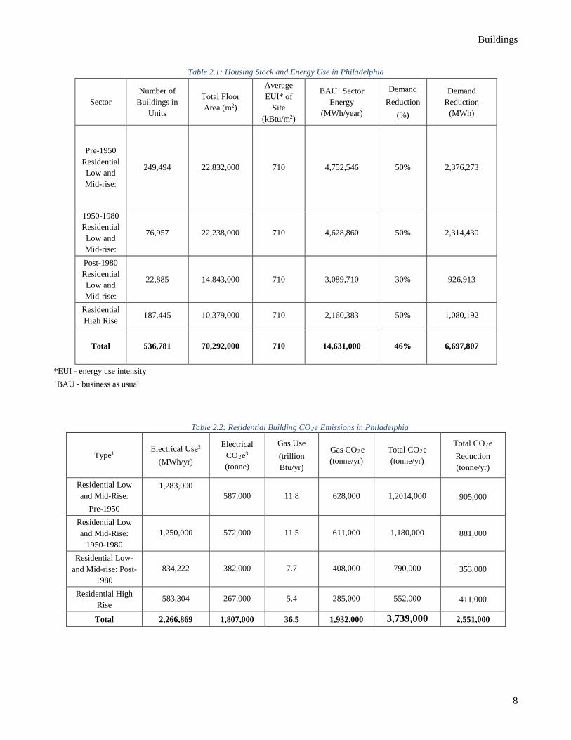
2.6 Residential Sector Residential energy use accounts for 13,482,750 MMBtu of total electricity use, 36,453,361 MMBtu of total gas use, and produces roughly 3.7 million tonnes CO2e/year. The total number of housing units was separated into 4 categories: mid-rise and low-rise buildings constructed before 1950, mid-rise and low-rise buildings constructed from 1950-1980, mid-rise and low-rise buildings constructed after 1980, and all high-rise buildings with high-rise comprising buildings greater than five stories high. The number of buildings in each residential sector was based on the United States Census Bureau data (Census 2015), while the floor areas of the different types of housing units were provided by the Mayor's Office of Sustainability (Mayor's Office of Sustainability, 2013b). Aggregate energy use for the residential sector was also supplied by the Mayor’s Office of Sustainability. However, energy use by category of housing unit was not available. The total energy use was divided among the four categories of residential housing in proportion to the floor area of each category, leading to a uniform energy use intensity of 66 kBtu/ft2 (Table 2.1). Baseline emissions (shown in Table 2.2) were then estimated by apportioning the energy use 73% towards gas and 27% towards electricity and applying emissions factors of 53 CO2e kg/MMBtu for gas use and 134 CO2e kg/MMBtu for electricity (EPA, 2015). Costs and energy use intensity reductions estimated for each of the categories of residential buildings are described below.

Buildings

8

Table 2.1: Housing Stock and Energy Use in Philadelphia

Sector Number of

Buildings in Units

Total Floor Area (m2)

Average EUI* of

Site (kBtu/m2)

BAU+ Sector Energy

(MWh/year)

Demand Reduction

(%)

Demand Reduction

(MWh)

Pre-1950 Residential Low and Mid-rise:

249,494 22,832,000 710 4,752,546 50% 2,376,273

1950-1980 Residential Low and Mid-rise:

76,957 22,238,000 710 4,628,860 50% 2,314,430

Post-1980 Residential Low and Mid-rise:

22,885 14,843,000 710 3,089,710 30% 926,913

Residential High Rise

187,445 10,379,000 710 2,160,383 50% 1,080,192

Total 536,781 70,292,000 710 14,631,000 46% 6,697,807

*EUI - energy use intensity +BAU - business as usual

Table 2.2: Residential Building CO2e Emissions in Philadelphia

Type1 Electrical Use2

(MWh/yr)

Electrical CO2e3 (tonne)

Gas Use (trillion Btu/yr)

Gas CO2e (tonne/yr)

Total CO2e (tonne/yr)

Total CO2e Reduction (tonne/yr)

Residential Low and Mid-Rise:

Pre-1950

1,283,000

587,000 11.8 628,000 1,2014,000 905,000

Residential Low and Mid-Rise:

1950-1980 1,250,000 572,000 11.5 611,000 1,180,000 881,000

Residential Low- and Mid-rise: Post-

1980 834,222 382,000 7.7 408,000 790,000 353,000

Residential High Rise

583,304 267,000 5.4 285,000 552,000 411,000

Total 2,266,869 1,807,000 36.5 1,932,000 3,739,000 2,551,000

Buildings

9

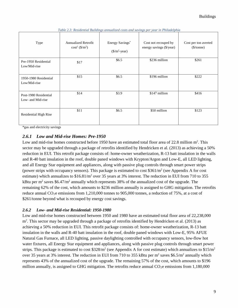
Table 2.3: Residential Buildings annualized costs and savings per year in Philadelphia

Type

Annualized Retrofit cost1 ($/m2)

Energy Savings*

($/m2-year)

Cost not recouped by energy savings ($/year)

Cost per ton averted ($/tonne)

Pre-1950 Residential Low/Mid-rise

$17 $6.5 $236 million $261

1950-1980 Residential Low/Mid-rise

$15 $6.5 $196 million $222

Post-1980 Residential Low- and Mid-rise

$14 $3.9 $147 million $416

Residential High Rise $11

$6.5 $50 million $123

*gas and electricity savings

2.6.1 Low and Mid-rise Homes: Pre-1950 Low and mid-rise homes constructed before 1950 have an estimated total floor area of 22.8 million m2. This sector may be upgraded through a package of retrofits identified by Hendricken et al. (2013) as achieving a 50% reduction in EUI. This retrofit package consists of: home-owner weatherization, R-13 batt insulation in the walls and R-40 batt insulation in the roof, double paned windows with Krypton/Argon and Low-E, all LED lighting, and all Energy Star equipment and appliances, along with passive plug controls through smart power strips (power strips with occupancy sensors). This package is estimated to cost $361/m2 (see Appendix A for cost estimate) which annualizes to $16.81/m2 over 35 years at 3% interest. The reduction in EUI from 710 to 355 kBtu per m2 saves $6.47/m2 annually which represents 38% of the annualized cost of the upgrade. The remaining 62% of the cost, which amounts to $236 million annually is assigned to GHG mitigation. The retrofits reduce annual CO2e emissions from 1,210,000 tonnes to 905,000 tonnes, a reduction of 75%, at a cost of $261/tonne beyond what is recouped by energy cost savings.

2.6.2 Low- and Mid-rise Residential: 1950-1980 Low and mid-rise homes constructed between 1950 and 1980 have an estimated total floor area of 22,238,000 m2. This sector may be upgraded through a package of retrofits identified by Hendricken et al. (2013) as achieving a 50% reduction in EUI. This retrofit package consists of: home-owner weatherization, R-13 batt insulation in the walls and R-40 batt insulation in the roof, double paned windows with Low-E, 95% AFUE Natural Gas Furnace, all LED lighting, passive daylighting controlled with occupancy sensors, low-flow hot water fixtures, all Energy Star equipment and appliances, along with passive plug controls through smart power strips. This package is estimated to cost $328/m2 (see Appendix A for cost estimate) which annualizes to $15/m2 over 35 years at 3% interest. The reduction in EUI from 710 to 355 kBtu per m2 saves $6.5/m2 annually which represents 43% of the annualized cost of the upgrade. The remaining 57% of the cost, which amounts to $196 million annually, is assigned to GHG mitigation. The retrofits reduce annual CO2e emissions from 1,180,000

Buildings

10

tonnes to 881,000 tonnes, a reduction of 75%, at a cost of $222/tonne beyond what is recouped by energy cost savings.

2.6.3 Low and Mid-Rise Homes: Post-1980 Low and mid-rise homes constructed after 1980 have an estimated total floor area of 14,843,000 m2. These more recently constructed homes tend to already have some ECMs, which makes it more difficult to achieve further reductions in energy consumption. Based on a review of the Hendricken et al. (2013) study it was determined that 50% reduction would be difficult to achieve, but a package capable of achieving 30% reduction in energy use was identified. This package consists of home-owner weatherization, R-13 batt insulation in the walls and white roof, 95% AFUE (annual fuel utilization efficiency) natural gas furnace, Energy Star central air conditioner (COP-5), all CFL lighting, passive lighting control using occupancy sensors, all Energy Star equipment and appliances, along with passive plug controls through smart power strips. This package is estimated to cost$302/m2 (see Appendix A for cost estimate) which annualizes to $14/m2 over 35 years at 3% interest. The reduction in EUI from 710 to 497 kBtu per m2 saves $3.9/m2 annually which represents 28% of the annualized cost of the upgrade. The remaining 72% of the cost, which amounts to $147 million annually, is assigned to GHG mitigation. The retrofits reduce annual CO2e emissions from 790,000 tonnes to 353,000 tonnes, a reduction of 45%, at a cost of $416/tonne beyond what is recouped by energy cost savings.

2.6.4 Residential High Rise Residential high rises have an estimated total floor area of 10,379,000 m2. This sector may be upgraded to achieve a 50% reduction in EUI through a package of retrofits identified by Hendricken (2014). This package consists of: R-9 + 5 inches of continuous insulation in the envelope and R-30 in the roof, with packaged terminal heat pumps with direct current cooling and electrical heating, passive daylighting controlled with occupancy sensors, low-flow water fixtures, all Energy Star equipment and appliances, and occupancy master control (a single switch that enables electrical devices in the home to be switched off upon leaving the residence). This package is estimated to cost $243/m2 (see Appendix A for cost estimate) which annualizes to $11/m2 over 35 years at 3% interest. The reduction in EUI from 710 to 355 kBtu per m2 saves $6.5/m2 annually which represents 59% of the annualized cost of the upgrade. The remaining 41% of the cost, which amounts to $50 million annually, is assigned to GHG mitigation. The retrofits reduce annual CO2e emissions from 552,000 tonnes to 411,000 tonnes, a reduction of 74%, at a cost of $123/tonne beyond what is recouped by energy cost savings.

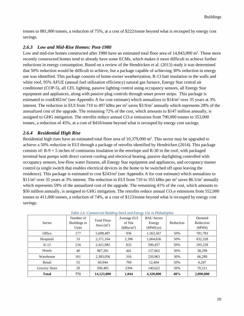
Table 2.4: Commercial Building Stock and Energy Use in Philadelphia

Sector Number of

Buildings in Units

Total Floor Area (m2)

Average EUI of Site

(kBtu/m2)

BAU Sector Energy

(MWh/yr) Reduction

Demand Reduction

(MWh) Office 177 5,698,487 936 1,563,567 50% 781,783

Hospitals 33 2,371,164 2,396 1,664,656 50% 832,328 K-12 216 2,421,982 832 590,457 50% 295,228

Hotels 40 987,281 441 127,662 30% 38,299 Warehouse 161 2,383,056 316 220,963 30% 66,289

Retail 55 60,944 700 12,494 50% 6,247 Grocery Store 29 200,485 2394 140,622 50% 70,311

Total 771 14,123,000 1,044 4,320,000 48% 2,090,000

Buildings

11

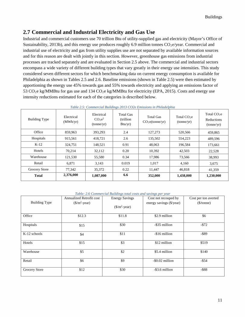
2.7 Commercial and Industrial Electricity and Gas Use Industrial and commercial customers use 70 trillion Btu of utility-supplied gas and electricity (Mayor’s Office of Sustainability, 2013b), and this energy use produces roughly 6.9 million tonnes CO2e/year. Commercial and industrial use of electricity and gas from utility supplies use are not separated by available information sources and for this reason are dealt with jointly in this section. However, greenhouse gas emissions from industrial processes are tracked separately and are evaluated in Section 2.5 above. The commercial and industrial sectors encompass a wide variety of different building types that vary greatly in their energy use intensities. This study considered seven different sectors for which benchmarking data on current energy consumption is available for Philadelphia as shown in Tables 2.5 and 2.6. Baseline emissions (shown in Table 2.5) were then estimated by apportioning the energy use 45% towards gas and 55% towards electricity and applying an emissions factor of 53 CO2e kg/MMBtu for gas use and 134 CO2e kg/MMBtu for electricity (EPA, 2015). Costs and energy use intensity reductions estimated for each of the categories is described below.

Table 2.5: Commercial Buildings 2013 CO2e Emissions in Philadelphia

Building Type Electrical (MWh/yr)

Electrical CO2e2

(tonne/yr)

Total Gas (trillion Btu/yr)

Total Gas CO2e(tonne/yr)

Total CO2e (tonne/yr)

Total CO2e Reductions (tonne/yr)

Office 859,963 393,293 2.4 127,273 520,566 459,865 Hospitals 915,561 418,721 2.6 135,502 554,223 489,596

K-12 324,751 148,521 0.91 48,063 196,584 173,661 Hotels 70,214 32,112 0.20 10,392 42,503 22,528

Warehouse 121,530 55,580 0.34 17,986 73,566 38,993 Retail 6,871 3,143 0.019 1,017 4,160 3,675

Grocery Store 77,342 35,372 0.22 11,447 46,818 41,359 Total 2,376,000 1,087,000 6.6 352,000 1,438,000 1,230,000

Table: 2.6 Commercial Buildings total costs and savings per year

Building Type Annualized Retrofit cost

($/m2-year) Energy Savings

($/m2-year)

Cost not recouped by energy savings ($/year)

Cost per ton averted ($/tonne)

Office $12.3 $11.8 $2.9 million $6

Hospitals $15 $30 -$35 million -$72

K-12 schools $4 $11 -$16 million -$89

Hotels $15 $3 $12 million $519

Warehouse $5 $2 $5.4 million $140

Retail $6 $9 -$0.02 million -$54

Grocery Store $12 $30 -$3.6 million -$88

Buildings

12

2.7.1 Office Buildings Philadelphia currently has 5.7 million m2 of office space. Office buildings account for 859,963 MWh of total electricity and 703,606 MWh of total gas usage, which results in an average EUI of 936 kBtu/m2 and produces 520,566 million metric tons of CO2e emissions per year.

This sector may be upgraded through a package of retrofits identified by Hendricken et al. (2012) as achieving 50% reduction in EUI. This retrofit package consists of: weatherization, double pane low emissivity windows, R-14 wall insulation, white roof, R-20 roof insulation, electrical heat pump with COP 3.3 for space heating and COP5 for space cooling, LED lights, passive daylighting controlled with occupancy sensors, light shelves, and task lighting where suitable. This package is estimated to cost $265/m2 (see Appendix A for cost estimate) which annualizes to $12.3/m2 over 35 years at 3% interest. The reduction in EUI from 936 to 468 kBtu/m2 saves $11.8/m2 annually which represents 96% of the annualized cost of the upgrade. The remaining 4% of the cost, which amounts to $2.9 million annually is assigned to GHG mitigation. The retrofits reduce annual CO2e emissions from 520,566 tonnes to 459,865 tonnes, a reduction of 88%, at a cost of $6/tonne.

2.7.2 Hospitals Philadelphia currently has 2,371,164 m2 of hospitals. Hospitals account for 915,561 MWh of total electricity usage and 2,599,141 MMBtu of total gas usage, which results in an average EUI of 2,396 kBtu/m2 and produces 554,223 tonnes of CO2e emissions.

This sector may be upgraded through a package of retrofits identified by ASHRAE (2012) as achieving 50% reduction in EUI. This retrofit package consists of R13 + 7.5 inches of continuous insulation in the walls, R-38 insulation in the floor, R-30 insulation in the roof, central air handling unit with 6.5 COP, 90% boiler efficiency and variable frequency drive on cooling tower fans, continuous air barrier, all LED lighting, pumps and fans fitted with variable frequency drives, and Energy Star equipment and appliances, including all traction elevators.

This package is estimated to cost $331/m2 (see Appendix A for cost estimate) which annualizes to $15/m2 over 35 years at 3% interest. The reduction in EUI from 2,396 to 1,198 kBtu/m2 saves $30/m2 annually which represents 150% of the annualized cost of the upgrade. The energy savings beyond the cost of the upgrade amount to $35 million annually and are assigned to GHG mitigation as a negative cost. The retrofits reduce annual CO2e emissions from 554,223 tonnes to 489,596 tonnes, a reduction of 88%, at a cost of $-72/tonne.

2.7.3 K-12 School Buildings Philadelphia currently has 26,070 kft2 of primary and secondary educational buildings. Educational buildings account for 1,108,384 MMBtu of total electricity usage and 906,860 MMBtu of total gas usage, which results in an average EUI of 832 kBtu/m2 and produces 196,534 tonnes of CO2e emissions.

This sector may be upgraded through a package of retrofits identified by ASHRAE (2011) as achieving a 50% reduction in EUI. This retrofit package consists of R13 + 7.5 inches of continuous insulation in the walls, R-38 insulation in the floor, and R-30 in the roof, ground source heat-pump, or a variable air volume air-handling system with a dedicated outdoor air system, T8 and T5 lighting with daylight zone controls, pumps and fans fitted with variable frequency drives, and Energy Star equipment and appliances.

This package is estimated to cost $88/m2 (see Appendix A for cost estimate) which annualizes to $4/m2 over 35 years at 3% interest. The reduction in EUI from 832 to 416 kBtu/m2 saves $11/m2 annually which represents 375% of the annualized cost of the upgrade. The energy savings beyond the cost of the upgrade amount to $16

Buildings

13

million annually and are assigned to GHG mitigation as a negative cost. The retrofits reduce annual CO2e emissions from 196,534 tonnes to 173,661 tonnes, a reduction of 88%, at a cost of -$89/tonne beyond.

2.7.4 Hotels Philadelphia currently has 10,627 kft2 of hotels. Hotels account for 617,780 MMBtu of total electricity use and 505,457 MMBtu of total gas use, which results in an average EUI of 441 kBtu/m2per square meter and produces 42,503 tonnes of CO2e emissions.

This sector may be upgraded through a package of retrofits identified by ASHRAE (2009) as achieving 30% reduction in EUI. This retrofit package consists of R-13 + 7.5 inches of continuous insulation in the walls, R-10 insulation in the floor, and R-20 in the roof, with electric 13.0 SEER heat pump cycle or 80% gas-fired furnace and 13 SEER Air Conditioner, T5HO, or T8 lighting with master control, and 90% efficient gas water heater.

This package is estimated to cost $326/m2 (see Appendix A for cost estimate) which annualizes to $15/m2 over 35 years at 3% interest. The reduction in EUI from 441 to 132.3 kBtu/m2per m2 saves $3/m2 annually which represents 20% of the annualized cost of the upgrade. The remaining 80% of the cost, which amounts to $2 million annually, is assigned to GHG mitigation. The retrofits reduce annual CO2e emissions from 42,503 tonnes to 22,528 tonnes, a reduction of 53%, at a cost of $519/tonne.

2.7.5 Warehouse Buildings Philadelphia currently has 25,651 kft2 of warehouse buildings. Warehouse buildings account for 324,774 MMBtu of total electricity use and 265,725 MMBtu of total gas use, , which results in an average EUI of 316 kBtu/m2MMBtu per thousand square meter and produces 73,566 tonnes of CO2e emissions.

This sector may be upgraded through a package of retrofits identified by ASHRAE (2008) as achieving 30% reduction in EUI. This retrofit package consists of R19 insulation in the walls, and R-20 insulation in the roof, with electric 13.0 SEER heat pump cycle or 80% gas-fired furnace and 13 SEER Air Conditioner, T5HO or T8 lighting with master control, and 90% efficient gas water heater.

This package is estimated to cost $101/m2 (see Appendix A for cost estimate) which annualizes to $5/m2 over 35 years at 3% interest. The reduction in EUI from 316 to 94.8 kBtu/m2 saves $2/m2 annually which represents 40% of the annualized cost of the upgrade. The remaining 60% of the cost, which amounts to $5.4 million annually is assigned to GHG mitigation. The retrofits reduce annual CO2e emissions from 73,566 tonnes to 38,993 tonnes, a reduction of 53%, at a cost of $140/tonne.

2.7.6 Retail Buildings Philadelphia currently has 6,561 kft2 of retail buildings. Retail buildings account for 414,769 MMBtu of total electricity use and 339,357 MMBtu of total gas usage, which results in an average EUI of 700 kBtu/m2per square meter and produces 4,160 tonnes of CO2e emissions. This sector may be upgraded through a package of retrofits identified by ASHRAE (2014) as achieving a 50% reduction in EUI. This retrofit package consists of R13 + 7.5 inches of continuous insulation in the walls, R-30 insulation in the floors, and R-20 insulation. in the roof, electric 13.0 SEER heat pump cycle or 80% gas-fired furnace and 13 SEER air conditioner, T5HO or T8 lighting with master control, 3% of roof area used for sky lights, and 90% efficient water heater.

This package is estimated to cost $120/m2 (see Appendix A for cost estimate) which annualizes to $6/m2 over 35 years at 3% interest. The reduction in EUI from 700 to 350 kBtu/m2Btu saves $9/m2 annually which represents

Buildings

14

150% of the annualized cost of the upgrade. The energy savings, which amount to $0.02 million annually are assigned to GHG mitigation as a negative cost. The retrofits reduce annual CO2e emissions from 4,160 tonnes to 3,675 tonnes, a reduction of 88%, at a cost of -$54/tonne.

2.7.7 Grocery Stores Philadelphia currently has 2,158 kft2 of grocery stores. Grocery Stores account for 263,945 MMBtu of total electricity use and 215,955 MMBtu of total gas uses, which results in an average EUI of 2,394 kBtu/m2per square meter and produces 46,818 tonnes of CO2e emissions. This sector may be upgraded through a package of retrofits identified by ASHRAE (2015) as achieving a 50% reduction in EUI. This retrofit package consists of R13 + 7.5 inches of continuous insulation in the walls, R-30 insulation in the floor, R-30 insulation in the roof, continuous air barrier with a distributed mixed air, single zone, variable air volume, direct expansion packaged roof top unit, LED lighting with occupancy master control, and a 94% efficient gas water heater (ASHRAE, 2015).

This package is estimated to cost $262/m2 (see Appendix A for cost estimate) which annualizes to $12/m2 over 35 years at 3% interest. The reduction in EUI from 2,394 to 1,197 kBtu/m2 saves $30/m2 annually which represents 250% of the annualized cost of the upgrade. The energy savings beyond the cost of the upgrade amount to $3.6 million annually and are assigned to GHG mitigation as a negative cost. The retrofits reduce annual CO2e emissions from 46,818 tonnes to 41,359 tonnes, a reduction of 88%, at a cost of -$88/tonne.

2.7.8 Other Commercial and Industrial Sectors The seven sectors considered above account for 14.7 trillion Btu or 21% of commercial and industrial use of utility-supplied electricity and gas. A total reduction of 1.2 million tonnes of CO2e emissions could be achieved by the retrofits identified here. If the proportionate reduction could be achieved in the remaining sectors, which account for 79% of energy use, then 5.9 million tonnes of CO2e emissions could be averted at an average cost of -$28/tonne.

2.8 Fuel Switching Rather than reducing demand one might substitute a low GHG source of energy for existing sources. Low-carbon electricity could be substituted for either gas or the existing electricity mix. The costs of a lower carbon electricity mix are considered in Chapter 4 and a scenario is developed in which a lower carbon electricity mix is substituted for the existing mix at a cost of $23 per tonne CO2e averted. This compares favorably with all of the residential demand reduction options considered here. Residential property owners might achieve greater impacts in purchasing low carbon electricity, rather than investing in highly ambitious upgrades to reduce their energy consumption by 50%. While the entire retrofit package needed to achieve 50% reduction may not be cost effective, specific ECMs may still be justified. Thus homeowners should carefully screen each ECM for cost effectiveness when making retrofit decisions.

Cost for carbon abatement in commercial buildings range from negative to very large positive values. Thus, depending on the specific commercial sector it may be more or less favorable to reduce demand as compared to switching to low carbon electricity. It is notable that the largest single sector considered here, office buildings, has a carbon abatement cost from energy efficiency of $6.35 per tonne. This is very favorable relative to alternative electricity and demonstrates how important opportunities for demand reduction exist in the buildings sector.

Buildings

15

Another fuel switching option would be to replace natural gas with low carbon electricity. Reducing an MMBtu of gas use would require 0.293 MWh if the electricity is used with equal efficiency to that of the gas. If the gas use is 70% effective and the electricity use is 100% effective, then only 0.21 MWh is required. At a cost of 136 $/MWh for nearly carbon free electricity (see Chapter 4), this would cost $27.89 or $16.50 more than an MMBtu of natural gas. It would avert 53 kg of carbon emissions if the electricity is completely carbon free for a cost of $311/tonne averted. Many other opportunities to abate carbon emissions are available at costs less than this, indicating that switching natural gas to low carbon electricity is not a favorable strategy at this point.

Generally energy efficiency has been seen as the most attractive emissions reduction strategies and to a considerable extent this remains true (Rumsey, 2015) as evidenced by the negative abatement costs for the retrofits considered here for hospitals, schools, groceries, and retail buildings. However, decreases in the price of renewable electricity have made some energy efficiency measures less attractive than switching to low-carbon electricity sources (Rumsey, 2015). In cases where the packages identified here are not cost effective, then this does not mean that energy efficiency investments should be avoided. Instead less expensive retrofit packages should be considered, even if these packages do not meet as ambitious goals as the packages considered here. Many demand reduction measures remain more cost effective than low-carbon electricity generation (Rumsey, 2015).

2.9 Total Emissions Reductions For the purpose of estimating whether an 80% reduction in building energy use is feasible, the demand reduction of 2.5 million tonnes from the residential analysis was summed with the demand reduction of 5.9 million tonnes obtained from the analysis of utility supplied power for commercial and industrial users to obtain a total reduction of 8.4 million tonnes or 80% of emissions from buildings, excluding process-based industrial emissions. This would require an overall energy use reduction of 47% and have an average cost of $55/tonne averted. This leads to the conclusion that reducing emissions by 80% from buildings is technically feasible through a program of ambitious retrofits that would reduce energy use intensity by 30-50%. The emissions reductions are greater than the decrease in energy use intensity as electricity savings would be applied exclusively to reduce the demand for fossil fuel derived electricity, allowing nuclear and renewables to form a larger portion of the electricity mix. If all electricity emissions were eliminated through the use of carbon-free electricity sources, then this would reduce emissions by 7 million tonnes/year or 66% and hence fall short of the 80% target. In addition to the elimination of carbon emissions from electricity use, a decrease in natural gas use of 41% would be required to reduce overall emissions in the building sector by 80%. In contrast, the target of 66% emissions reductions, which would allow Philadelphia to meet the U.S. average per capita emissions target for 2050, corresponds very closely to the emissions reduction that could be achieved by switching to carbon-free electricity.

It reality the demand reductions considered here should be pursued selectively. In cases where the packages of ECMs considered here are not cost-effective relative to fuel switching, then the packages should be disaggregated and subsets of ECMs that are cost-effective can be implemented.

2.10 Impact on Electricity Demand As discussed in Section 2.8., reduction in electricity demand is an alternative to the development of low-carbon electricity generation capacity. If the full 80% reduction in GHG emissions were implemented as described in Section 2.9 then the electricity demand averted would be 7,290,000 MWh/year or 51% of the city’s current annual electricity use. If only the portion of demand reduction that is more cost-effective than the $23/tonne cost

Buildings

16

of emissions reductions for the low-carbon electricity mix developed in Chapter 4, is implemented (that is, retrofits of schools, hospitals, groceries, retail stores, and offices), then the demand reduction amounts to 1,090,000 MWh/year or 7.6% of the city’s demand. It is acknowledged that demand reductions can lead to lower prices that stimulate energy use and ultimately displace consumption to other sectors and uses, a phenomenon often referred to as rebound. One study estimated that energy efficiency measures in buildings might lead to a 20% rebound effect (that is, 20% of the demand reductions are offset by demand increases for other energy uses) (Copenhagen Economics 2012). In an 80 by 50 scenario, energy costs might actually increase despite demand reductions (for example, an aggressive de-carbonization option considered in Chapter 4 involves roughly 10% higher electricity costs) which would remove that classic impetus for rebound, lower prices. However, 80 by 50 scenarios involve substantial changes to energy consumption patterns and the precise impacts cannot realistically be foreseen at this time. For example, it is possible that increased electricity demand in the transportation sector due to demands from plug-in electric hybrid vehicles could be on the same scale as the demand reduction achieved in the building sector (see Chapter 3 for transportation scenarios).

Transportation

17

3 TRANSPORTATION 3.1 Abstract The aim of this report is to investigate the possibility of achieving a reduction of 80% in transport emissions in Philadelphia compared to current emissions. Our base case is 2012, which coincides with the most recent Household Travel Survey (HTS) that constitutes a fundamental building block of our analysis. Using trip information in the HTS, we first quantified daily lifecycle emissions generated by the Greater Philadelphia Region in 2012 and projected these emissions to 2050 accounting for population growth and future trends in vehicle technology. We then extracted emissions associated with the City of Philadelphia. We also investigated the effects of twelve different policy scenarios on regional GHG emissions in 2050 compared to 2012. Our scenarios incorporate the effects of alternative fuels as well as mode shift towards public transit and active transportation. We observe that reductions of 80% are technically feasible and that large reductions in emissions can only be achieved through a combination of active transportation, cleaner fuels for public transit vehicles, and a significant market penetration of battery electric vehicles. Additional electricity demand associated with greater use of electric vehicles could amount to 10.8 TWh/year, 92% of which would be drawn from outside the city limits. Costs of abatement are difficult to determine but plug-in hybrid electric vehicles constitute a substantial portion of the emissions reductions considered here and have been estimated to have an abatement cost of $90/tonne in the year 2020.

Transportation

18

3.2 Introduction The transportation sector accounts for about 19% of Philadelphia’s emissions (Mayor’s Office of Sustainability, 2015b). The significant contribution of transportation to greenhouse gas emissions (GHG) is a subject that has received much attention. The literature swells with recent research demonstrating the role and potential of urban transportation in the reduction of anthropogenic GHG emissions. In 2012, transportation in the US was responsible for 1,837 Teragrams of GHG emissions, which account for 28% of the total GHG emissions. Among this portion, 84% of the transportation GHG emissions are associated with road transportation with light duty vehicles being responsible for 62%, and medium and heavy duty trucks responsible for 22% (Office of Transportation and Air Quality, 2015). The climate change and sustainability agenda have added a new dimension to transport policy in metropolitan areas throughout North America and around the world. In light of the recent challenges brought by global warming issues and the need to curb environmental degradation and promote sustainable transportation in urban areas, planners and policy-makers are faced with a major challenge. This challenge involves the development and implementation of transport policy that can reduce GHGs and air pollutant emissions while at the same time promoting economic growth and offering new transportation alternatives ranging from the promotion of alternative fuels to investments in transit infrastructure and encouraging the use of active transportation. The City of Philadelphia is committed to achieving a significant decrease in transport emissions of GHG by 2050 compared to current emissions and is interested in investigating the effects of various strategies in reducing emissions by 80% in 2050. .

Across the US, a large number of metropolitan areas have recently gone through an exercise of estimating the carbon footprint of urban transportation and investigating the reduction potential of various transportation alternatives.

New York City has recently set a goal of reducing total GHG emissions by 90% in 2050 compared to 2010, while for transportation the target is to reduce emissions by 54% (Urban Green Council, 2013). In 2010, New York’s annual GHG emissions from transportation were approximately 11.3 million tons of which 68% were attributed to gasoline passenger cars and 8.33% to gasoline light-duty trucks, and the remaining from other modes of transportation. By 2050 New York has a target of reducing total transportation GHG emissions by 73% focusing on the (1) electrification and expansion of passenger and freight rail, (2) conversion of on-road vehicles to electric, hybrid, and turbo diesel vehicles; and (3) redistribution of public transit passengers to more energy efficient modes such as electric trolley buses and electric rail.

The City of Fort Collins, Colorado committed to reduce GHG emissions by 80% in 2050 compared to 2005. In 2012, the total annual fuel consumption of transportation fuels was estimated at 58 million gallons, and in 2030 it is projected to reach 45 million gallons under business as usual (BAU) conditions; this decrease is associated with the expected improvements in vehicle fuel efficiency. Compared to 2030-BAU conditions, the authors estimated potential reductions in total fuel consumption of about 48%, leaving a net benefit of $480 million in reduced vehicle costs and maintenance (Rocky Mountain Institute, 2014). This reduction can be achieved by (1) decreasing personal vehicle mileage, (2) using electric and fuel-efficient vehicles, (3) converting heavy-duty trucks to natural gas and bio fuels, and (4) using battery electric vehicles

The state of California has also set a target to reduce its GHG emissions by 80% in 2050 compared to 1990. A recent study estimated that California currently generates about 440 million tons of GHG (in 2010) and estimated about 40 million tons in 2050, a reduction of 83.33% in 40 years (Yang, Yeh, Zakerinia, Ramea, &

Transportation

19

McCollum, 2015). Such a reduction rests upon investments in low-carbon electricity, alternative fueled vehicles, and efficiency improvements across many sectors.

The City of Boston has also set a reduction target of 80% by 2050 compared to 2005 emissions. It was estimated that between 2005 and 2013, total GHG emissions have been reduced by 17%, mostly due to a cleaner electric grid (City of Boston, 2015a, City of Boston 2015b). Transportation emissions were reduced by 8.3%. The study also highlights the challenges behind achieving 2050 targets and stresses the importance of energy and transportation infrastructure, including improved fuel economy, reduced vehicle miles traveled, car/ride share, parking freeze, and improved transit.

Finally, the Delaware Valley Regional Planning Commission (DVRPC) has set a target of reducing regional GHG emissions to 50 percent below 2005 levels by the year 2035 and calls for a 60 percent drop by 2040 in order to achieve an 80 percent reduction by 2050. In July 2013, DVRPC launched a plan entitled: “Connections 2040: Plan for Greater Philadelphia”. The region was estimated to generate 26.1 million tons of GHG in 2010 from the “mobile energy use” sector which includes on-road motor vehicles, rail, marine, aviation, and off-road motorized vehicles and equipment (DVRPC, 2014b). Between 2005 and 2010, transportation-related GHG emissions decreased from 27.3 million tons to 26.1 million tons, a reduction of 4.4%. On-road vehicles are responsible for around 80% of total transportation emissions, and between 2005 and 2010 the reduction was only by 1%. In order to achieve the target reductions, DVRPC proposes road and transit expansions and operational improvements (DVRPC, 2014a). In 2012, the local transit provider, Southeastern Pennsylvania Transport Authority (SEPTA), initiated an energy action plan to reduce its energy intensity by 10% and its annual GHG intensity by 5% by 2015 compared to 2009 (SEPTA, 2012). On a per passenger basis, emissions decreased by about 4.25% per year between 2009 and 2012 (SEPTA, 2015). A similar trend was also observed for total emissions, whereby total GHG emissions generated by SEPTA buses decreased from 0.421 million tons to 0.416 million tons between 2009 and 2013.

The aim of this report is to investigate the possibility of achieving a reduction of 80% in transport emissions in Philadelphia compared to current emissions. Our base case is 2012, which coincides with the most recent Household Travel Survey (HTS) that constitutes a fundamental building block of our analysis. In this respect, it is important to note that our analysis was restricted to daily household travel and did not include commercial vehicle movements. We also did not account for emissions from air travel. Therefore, our inventory is expected to underestimate real emissions. Yet, since municipal transport policies are most likely to target daily household travel decisions, we can demonstrate the effects of strategies on GHG emissions. Using the trip diary information in the HTS, we first quantified daily lifecycle emissions generated by the Greater Philadelphia Region in 2012 and projected these emissions to 2050 accounting for population growth and projected trends in vehicle technology. We then extracted emissions associated with the City of Philadelphia. We also investigated the effects of twelve different policy scenarios in reducing GHG emissions in 2050 compared to 2012. Our scenarios incorporate the effects of alternative fuels as well as mode shift towards public transit and active transportation.

3.3 Methodology The methodology adopted to calculate GHG emissions from the transportation sector in Philadelphia includes three main elements: 1) processing transportation data, 2) developing emission factors (EFs) per vehicle and mile travelled, and 3) merging travel data with EFs in order to estimate total emissions. It is important to note at the onset that the GHG emissions were estimated only for household travel and did not include commercial

Transportation

20

vehicle movements. Because of the large number of trips originating or destined outside of the city, our methodology included estimating transportation emissions generated by residents of Southern New Jersey and Southeastern Pennsylvania; the emissions associated with the city were then extracted and compared with the regional emissions.

3.3.1 Trip information We obtained information about trips in the region from the 2012 HTS sponsored by the DVRPC, the Metropolitan Planning Organization (MPO) for the Greater Philadelphia Region. The HTS is a trip diary survey whereby individuals and households complete a diary of all trips conducted within a day. The survey targets a random sample of the region’s population and is conducted approximately every 10 years (DVRPC, 2015).

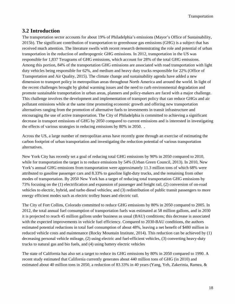
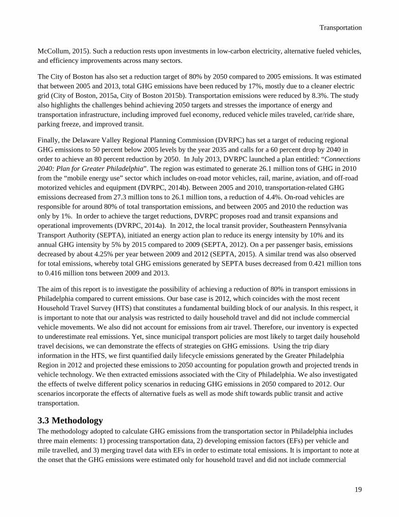
In the most recent survey, conducted in 2012, travel data for 20,216 individuals (and 9,235 households) were collected. We obtained disaggregate, individual-level data including zone of residence, and attributes for each trip including: origin and destination, mode used, vehicle type (model year and make if a private vehicle was used), modeled trip distance, and modeled travel time and average speed. We also obtained two different factors or weights associated with each trip: one weight which allowed us to expand the survey sample up to the total population and another which allowed us to correct for under-reported trip lengths. Table 3.1 provides the total numbers of individuals, households, and trips included in the survey. Based on the trip records included within the survey, 80% of the trips are conducted using private vehicles while 5% rely on public transit. Figure 3.1 presents the distribution of travel modes.

Table 3.1: 2012 Household Travel Survey (HTS) public database

Total number of households 9,235

Total number of individuals 20,216

Average household size 2.19

Total number of trips per day 61,725

Average number of individuals per household 2.19

Average number of trips per household per day 8.87

Average number of trips per individual per day 4.05

Average person weight 264.63

Average trip factor 1.145

Transportation

21

Figure 3.1: Distribution of travel modes across the 2012 Household Travel Survey (HTS)

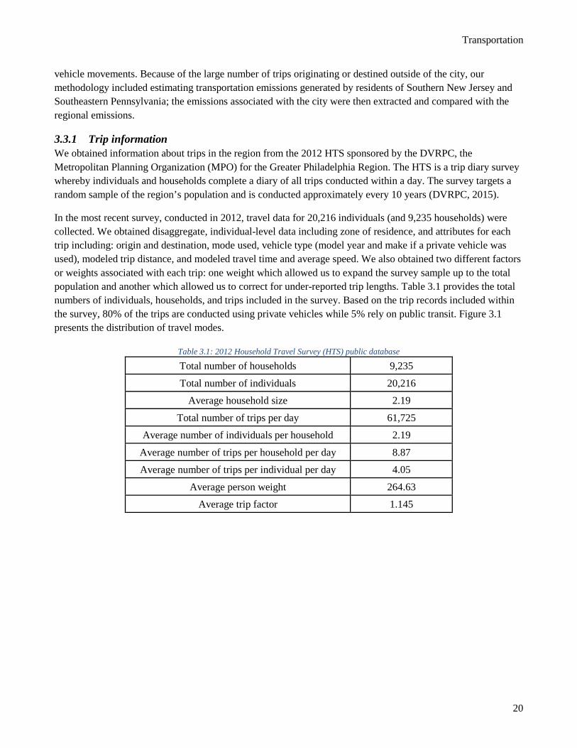
Mean trip lengths (in miles and minutes) across the major modes (private vehicle, public transit, school bus, walk, and bike) are summarized in Figure 3.2. While the mean trip distance for public transit is slightly lower than that of private vehicles, the mean duration is almost twice on public transit compared to the private vehicle. Figure 3.3 illustrates that over 30% of the trips conducted by private vehicles are shorter than 11 minutes. This relatively short travel time by car indicates that it could be possible to shift some of these trips to public transit without a large negative effect on the duration of the trip. Of course, such a shift depends on the origin of these trips (e.g. whether they start at a location served by transit) and their place within an individual’s daily tour (e.g. if they are followed by a trip that involves serving a dependent).

Figure 3.2: Distribution of trip lengths across major modes

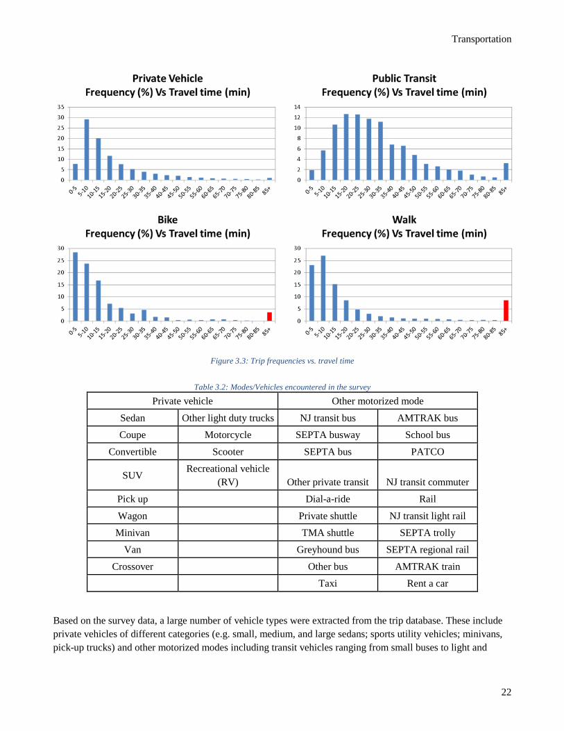
Transportation

22

Figure 3.3: Trip frequencies vs. travel time

Table 3.2: Modes/Vehicles encountered in the survey

Private vehicle Other motorized mode

Sedan Other light duty trucks NJ transit bus AMTRAK bus

Coupe Motorcycle SEPTA busway School bus

Convertible Scooter SEPTA bus PATCO

SUV Recreational vehicle

(RV) Other private transit NJ transit commuter

Pick up Dial-a-ride Rail

Wagon Private shuttle NJ transit light rail

Minivan TMA shuttle SEPTA trolly

Van Greyhound bus SEPTA regional rail

Crossover Other bus AMTRAK train

Taxi Rent a car

Based on the survey data, a large number of vehicle types were extracted from the trip database. These include private vehicles of different categories (e.g. small, medium, and large sedans; sports utility vehicles; minivans, pick-up trucks) and other motorized modes including transit vehicles ranging from small buses to light and

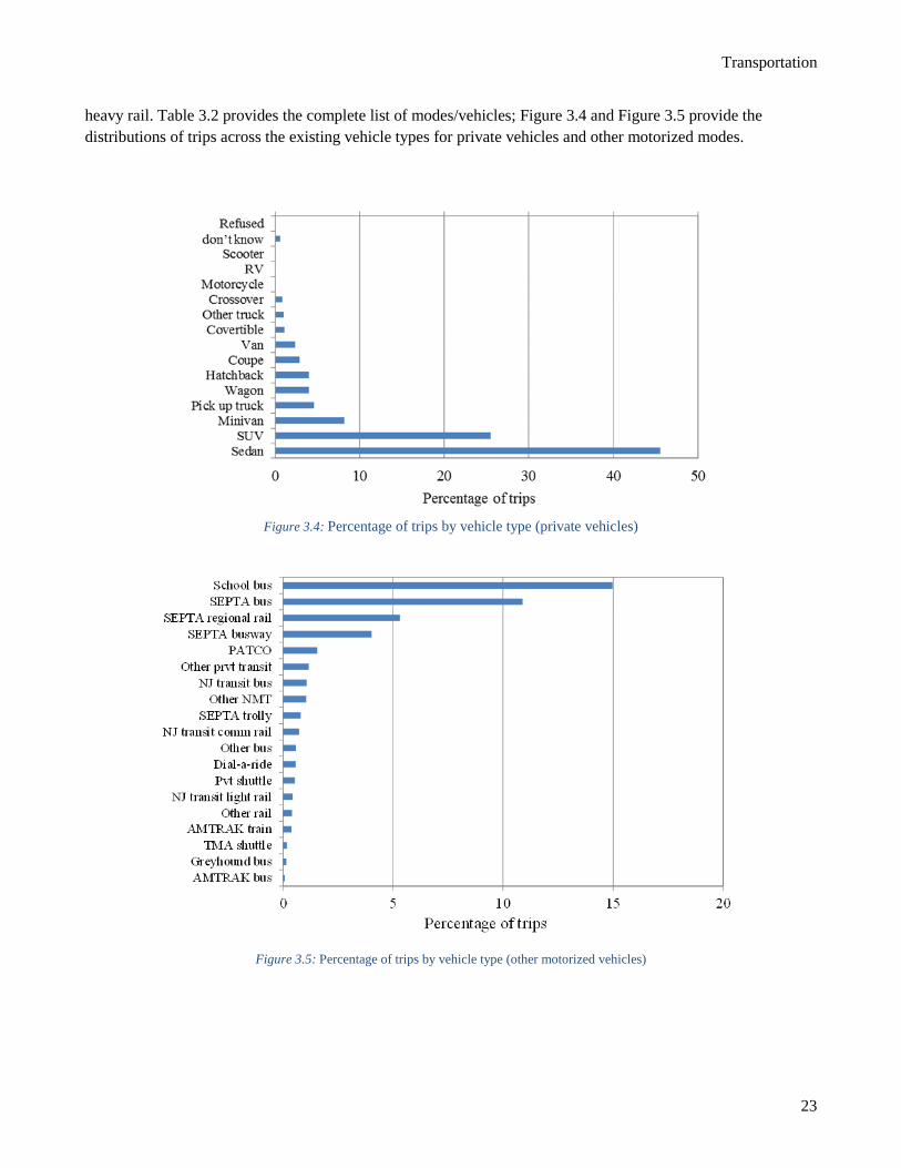
Transportation

23

heavy rail. Table 3.2 provides the complete list of modes/vehicles; Figure 3.4 and Figure 3.5 provide the distributions of trips across the existing vehicle types for private vehicles and other motorized modes.

Figure 3.4: Percentage of trips by vehicle type (private vehicles)

Figure 3.5: Percentage of trips by vehicle type (other motorized vehicles)

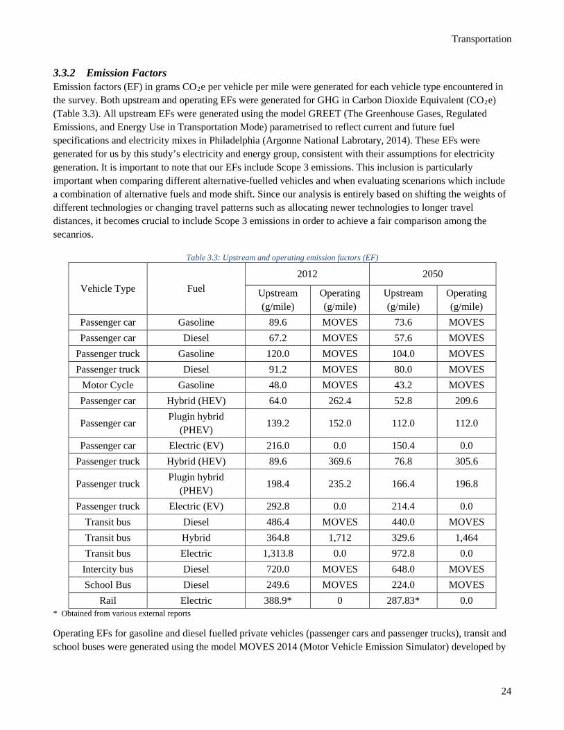
Transportation

24

3.3.2 Emission Factors Emission factors (EF) in grams CO2e per vehicle per mile were generated for each vehicle type encountered in the survey. Both upstream and operating EFs were generated for GHG in Carbon Dioxide Equivalent (CO2e) (Table 3.3). All upstream EFs were generated using the model GREET (The Greenhouse Gases, Regulated Emissions, and Energy Use in Transportation Mode) parametrised to reflect current and future fuel specifications and electricity mixes in Philadelphia (Argonne National Labrotary, 2014). These EFs were generated for us by this study’s electricity and energy group, consistent with their assumptions for electricity generation. It is important to note that our EFs include Scope 3 emissions. This inclusion is particularly important when comparing different alternative-fuelled vehicles and when evaluating scenarions which include a combination of alternative fuels and mode shift. Since our analysis is entirely based on shifting the weights of different technologies or changing travel patterns such as allocating newer technologies to longer travel distances, it becomes crucial to include Scope 3 emissions in order to achieve a fair comparison among the secanrios.

Table 3.3: Upstream and operating emission factors (EF)

Vehicle Type Fuel 2012 2050

Upstream (g/mile)

Operating (g/mile)

Upstream (g/mile)

Operating (g/mile)

Passenger car Gasoline 89.6 MOVES 73.6 MOVES Passenger car Diesel 67.2 MOVES 57.6 MOVES

Passenger truck Gasoline 120.0 MOVES 104.0 MOVES Passenger truck Diesel 91.2 MOVES 80.0 MOVES

Motor Cycle Gasoline 48.0 MOVES 43.2 MOVES Passenger car Hybrid (HEV) 64.0 262.4 52.8 209.6

Passenger car Plugin hybrid

(PHEV) 139.2 152.0 112.0 112.0

Passenger car Electric (EV) 216.0 0.0 150.4 0.0 Passenger truck Hybrid (HEV) 89.6 369.6 76.8 305.6

Passenger truck Plugin hybrid

(PHEV) 198.4 235.2 166.4 196.8

Passenger truck Electric (EV) 292.8 0.0 214.4 0.0 Transit bus Diesel 486.4 MOVES 440.0 MOVES Transit bus Hybrid 364.8 1,712 329.6 1,464 Transit bus Electric 1,313.8 0.0 972.8 0.0

Intercity bus Diesel 720.0 MOVES 648.0 MOVES School Bus Diesel 249.6 MOVES 224.0 MOVES

Rail Electric 388.9* 0 287.83* 0.0 * Obtained from various external reports

Operating EFs for gasoline and diesel fuelled private vehicles (passenger cars and passenger trucks), transit and school buses were generated using the model MOVES 2014 (Motor Vehicle Emission Simulator) developed by

Transportation

25

EPA’s Office of Transportation and Air Quality (OTAQ) (EPA, 2014). We chose to use MOVES to estimate operating emissions of gasoline- and diesel-fuelled vehicles because MOVES accounts for the effect of speed on emissions. This is particularly important for private vehicles whereby the emissions of trips conducted during congested vs. uncongested periods would be different. Operating emissions of alterative-fuelled vehicles were estimated using GREET since MOVES does not calculate EFs for these vehicle types. In this case, EFs were not speed dependent but were estimated for a single average speed.

The various vehicles types listed in Table 3.2 were consolidated into a smaller set of vehicles for emission estimation purposes. For example, private vehicles were divided into passenger cars, passenger trucks, and motorcycles. Other vehicles included transit buses, school buses, intercity buses and rail (electric and diesel). The final consolidated list of vehicles encountered in the 2012 survey is presented in Table 3.3.

It is important to note that we did not add new vehicle/fuel types to the list in 2050. Our 2050 EFs are based on projected improvements in vehicle technology and in electricity mix in Philadelphia under business as usual conditions and are derived for the existing vehicle types in 2012. In our scenario analysis, we investigate the effects of greater market penetration for these same vehicles with the most plausible emissions in 2050 assuming a business as usual evolution in the mix for electricity generation. We also investigate the effects of this same market penetration rate with improved EFs assuming a more optimistic projection for electricity generation.

In this context, it is important to mention the assumptions behind the electricity mix in 2050, which formed the basis for the GREET model emission factors for electric vehicles (EV), plug-in hybrid vehicles (PHEV), hybrid electric vehicles (HEV) and electric transit buses. The electricity mix in the 2012 base case scenario reflects current conditions in Philadelphia, which sources its electricity from the RFC regional electricity grid mix (see Chapter 4). The business as usual projection for both 2012 and 2050 assume the fuel mix of: 1% residual oil and biomass, 2% renewables, 23.6% coal, 26.9% nuclear, and 45.5% natural gas. Finally, a more optimistic electricity mix for 2050 was developed including: 0% coal, 1% residual oil, 10% natural gas, 40% nuclear, and 49% renewables.

3.3.3 Estimation of Base Case (2012) and Business as Usual (2050) Emissions Base case emissions were calculated for each trip based on the mode, vehicle type, and average speed (when calculating operating emissions of gasoline and diesel vehicles). For each trip, emissions were first multiplied by a correction factor (accounting for under-reporting of trips), then multiplied by trip-based weights representing each trip’s weight in the total population (Figure 3.6). Total emissions were then aggregated per traffic analysis zone (TAZ) using two different schemes:

1) Summing all individual emissions and associating them with the household residential location. This aggregation provides us with daily emissions generated by residents of each TAZ irrespective of where these emissions occur.

2) For each trip, emissions are divided in two; one half is assigned to the TAZ of origin and another to the TAZ of destination. This aggregation provides us with a “proxy” for the location of daily emissions.

In the two aggregation schemes, we investigated the regional emissions as well as the emissions associated with the City of Philadelphia. As such, method 1 provided us with the emissions generated by the residents of the city throughout their daily trips while the second method provided us with the emissions “occurring” in the city both from the residents and travelers living outside the city and visiting the city (for business, leisure, shopping, etc.)

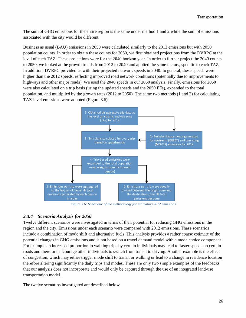
Transportation

26

The sum of GHG emissions for the entire region is the same under method 1 and 2 while the sum of emissions associated with the city would be different.

Business as usual (BAU) emissions in 2050 were calculated similarly to the 2012 emissions but with 2050 population counts. In order to obtain these counts for 2050, we first obtained projections from the DVRPC at the level of each TAZ. These projections were for the 2040 horizon year. In order to further project the 2040 counts to 2050, we looked at the growth trends from 2012 to 2040 and applied the same factors, specific to each TAZ. In addition, DVRPC provided us with their projected network speeds in 2040. In general, these speeds were higher than the 2012 speeds, reflecting improved road network conditions (potentially due to improvements to highways and other major roads). We used the 2040 speeds in our 2050 analysis. Finally, emissions for 2050 were also calculated on a trip basis (using the updated speeds and the 2050 EFs), expanded to the total population, and multiplied by the growth rates (2012 to 2050). The same two methods (1 and 2) for calculating TAZ-level emissions were adopted (Figure 3.6)

Figure 3.6: Schematic of the methodology for estimating 2012 emissions

3.3.4 Scenario Analysis for 2050 Twelve different scenarios were investigated in terms of their potential for reducing GHG emissions in the region and the city. Emissions under each scenario were compared with 2012 emissions. These scenarios include a combination of mode shift and alternative fuels. This analysis provides a rather coarse estimate of the potential changes in GHG emissions and is not based on a travel demand model with a mode choice component. For example an increased proportion in walking trips by certain individuals may lead to faster speeds on certain roads and therefore encourage other individuals to switch from transit to driving. Another example is the effect of congestion, which may either trigger mode shift to transit or walking or lead to a change in residence location therefore altering significantly the daily trips and modes. These are only two simple examples of the feedbacks that our analysis does not incorporate and would only be captured through the use of an integrated land-use transportation model.

The twelve scenarios investigated are described below.

Transportation

27

Scenario 1: all individuals with a total daily travel distance below 5 miles would convert all their trips to walking. While this scenario does not take into account the locations of the trips or whether they involve serving a dependent, it provides an optimistic estimate of anticipated GHG reductions if a growing proportion of the population switched to active transportation.

Scenario 2: all individuals with a total daily travel distance below 10 miles would convert all their trips to cycling. This scenario does not take into account the presence of bicycle facilities, the location of trips, the age of the individual making the trip, or whether the trip involves serving a dependent.

Scenario 3: all drivers of private vehicles who conduct only two trips per day (starting and ending at home) would convert to public transit. It was observed that 25% of the individuals in the survey conduct only two trips per day by private vehicle. This scenario considers both the decrease in private vehicle emissions and the increase in transit emissions. It is assumed that suitable public transit options are available.

Scenario 4: all drivers of private vehicles with the 80th percentile daily travel distance (more than 41.28 miles driven per day) replace their current private vehicle by a PHEV. The EF for PHEV is presented in Table 3.3 (112 g/veh.mile upstream and 112 g/veh.mile operating emissions in 2050) and assumes business as usual projections for electricity mix. In this scenario we also calculated the total electricity consumption.

Scenario 5: all drivers of private vehicles with the 60th percentile daily travel distance (more than 26.21 miles driven per day) replace their current private vehicle by a PHEV. The EF for PHEV is presented in Table 3.3 (112 g/veh.mile upstream and 112 g/veh.mile operating emissions in 2050) and assumes business as usual projections for electricity mix. In this scenario we also calculated the total electricity consumption.

Scenario 6: Scenario 4 was repeated assuming a more optimistic assumption for the electricity mix in 2050 leading to lower emissions for PHEV (36.8 g/veh.mile upstream and 112 g/veh.mile operating).

Scenario 7: is a combination of Scenarios 3 and 4 whereby “extreme commuters” replace their vehicles by PHEV and the share of transit increases. As with Scenario 3, increased emissions from public transit are considered and suitable public transit options are assumed to be available.

Scenario 8: Scenario 5 was repeated assuming a more optimistic scenario for electricity mix in 2050 leading to lower emissions for PHEV (36.8 g/veh.mile upstream and 112 g/veh.mile operating).

Scenario 9: Scenario 7 was repeated while considering all SEPTA buses as electric (with a 972.8 g/veh.mile upstream and 0 g/veh.mile operating emissions).

Scenario 10: Scenarios 3 and 8 were combined considering all SEPTA transit buses as electric (with a 972.8 g/veh.mile upstream and 0 g/veh.mile operating emissions).

Scenario 11: is a combination of Scenarios 1, 2 and 10 whereby walking and biking are coupled with other improvements (drivers of private vehicles with the 60th percentile daily travel distance replace their current private vehicle by a PHEV, optimistic electricity mix assumption, and electric SEPTA buses).

Scenario 12: Scenario 11 was repeated while replacing all PHEV cars as battery electric cars having 150 g/veh.mile upstream and 0 g/veh.mile operating emissions.

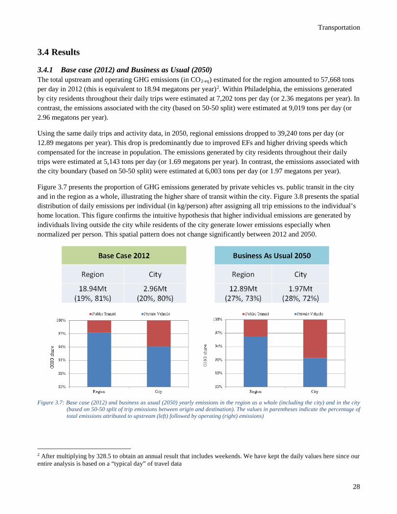
Transportation

28

3.4 Results

3.4.1 Base case (2012) and Business as Usual (2050) The total upstream and operating GHG emissions (in CO2-eq) estimated for the region amounted to 57,668 tons per day in 2012 (this is equivalent to 18.94 megatons per year)2. Within Philadelphia, the emissions generated by city residents throughout their daily trips were estimated at 7,202 tons per day (or 2.36 megatons per year). In contrast, the emissions associated with the city (based on 50-50 split) were estimated at 9,019 tons per day (or 2.96 megatons per year).

Using the same daily trips and activity data, in 2050, regional emissions dropped to 39,240 tons per day (or 12.89 megatons per year). This drop is predominantly due to improved EFs and higher driving speeds which compensated for the increase in population. The emissions generated by city residents throughout their daily trips were estimated at 5,143 tons per day (or 1.69 megatons per year). In contrast, the emissions associated with the city boundary (based on 50-50 split) were estimated at 6,003 tons per day (or 1.97 megatons per year).

Figure 3.7 presents the proportion of GHG emissions generated by private vehicles vs. public transit in the city and in the region as a whole, illustrating the higher share of transit within the city. Figure 3.8 presents the spatial distribution of daily emissions per individual (in kg/person) after assigning all trip emissions to the individual’s home location. This figure confirms the intuitive hypothesis that higher individual emissions are generated by individuals living outside the city while residents of the city generate lower emissions especially when normalized per person. This spatial pattern does not change significantly between 2012 and 2050.

Figure 3.7: Base case (2012) and business as usual (2050) yearly emissions in the region as a whole (including the city) and in the city

(based on 50-50 split of trip emissions between origin and destination). The values in parentheses indicate the percentage of total emissions attributed to upstream (left) followed by operating (right) emissions)

2 After multiplying by 328.5 to obtain an annual result that includes weekends. We have kept the daily values here since our entire analysis is based on a “typical day” of travel data

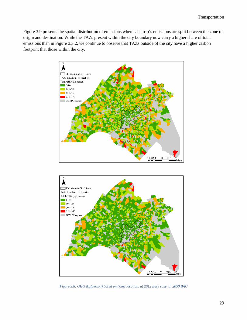
Transportation

29

Figure 3.9 presents the spatial distribution of emissions when each trip’s emissions are split between the zone of origin and destination. While the TAZs present within the city boundary now carry a higher share of total emissions than in Figure 3.3.2, we continue to observe that TAZs outside of the city have a higher carbon footprint that those within the city.

Figure 3.8: GHG (kg/person) based on home location. a) 2012 Base case. b) 2050 BAU

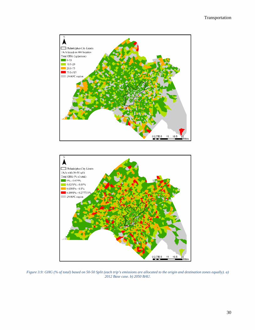
Transportation

30

Figure 3.9: GHG (% of total) based on 50-50 Split (each trip’s emissions are allocated to the origin and destination zones equally). a)

2012 Base case. b) 2050 BAU.

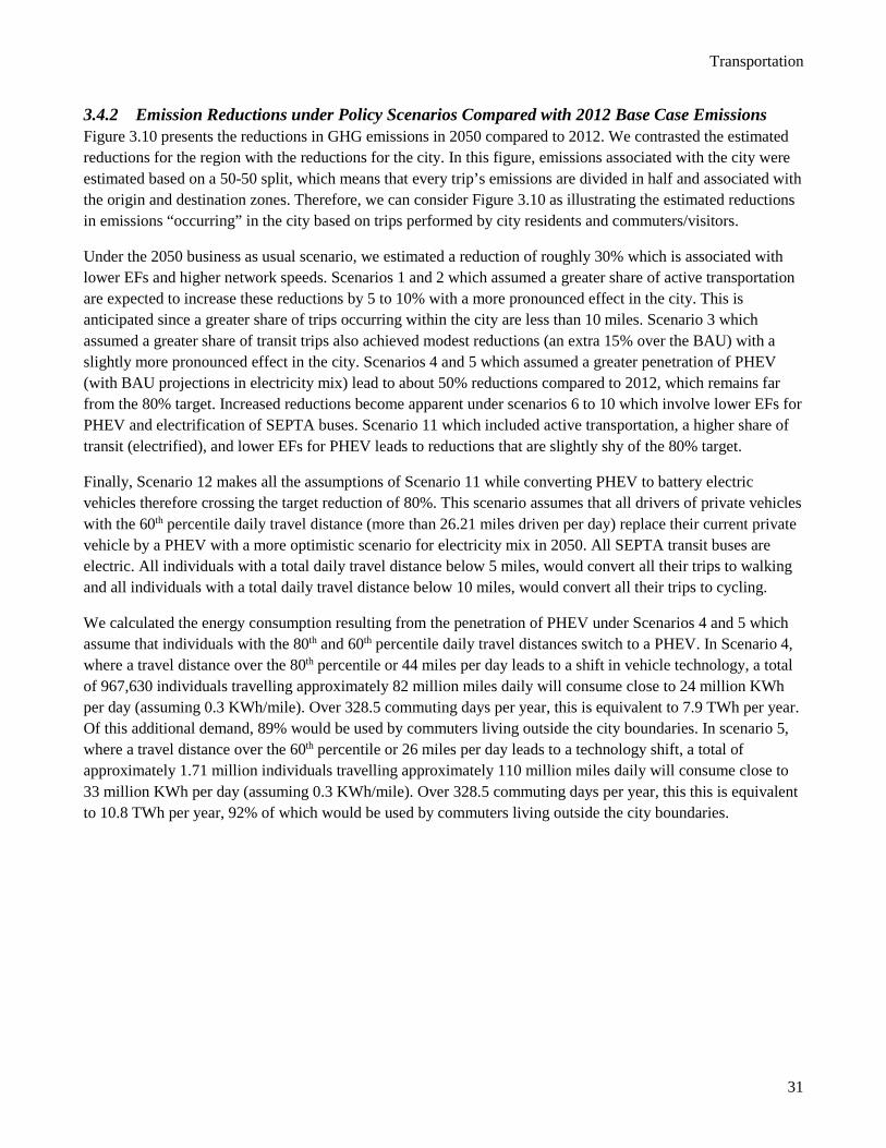
Transportation

31

3.4.2 Emission Reductions under Policy Scenarios Compared with 2012 Base Case Emissions Figure 3.10 presents the reductions in GHG emissions in 2050 compared to 2012. We contrasted the estimated reductions for the region with the reductions for the city. In this figure, emissions associated with the city were estimated based on a 50-50 split, which means that every trip’s emissions are divided in half and associated with the origin and destination zones. Therefore, we can consider Figure 3.10 as illustrating the estimated reductions in emissions “occurring” in the city based on trips performed by city residents and commuters/visitors.

Under the 2050 business as usual scenario, we estimated a reduction of roughly 30% which is associated with lower EFs and higher network speeds. Scenarios 1 and 2 which assumed a greater share of active transportation are expected to increase these reductions by 5 to 10% with a more pronounced effect in the city. This is anticipated since a greater share of trips occurring within the city are less than 10 miles. Scenario 3 which assumed a greater share of transit trips also achieved modest reductions (an extra 15% over the BAU) with a slightly more pronounced effect in the city. Scenarios 4 and 5 which assumed a greater penetration of PHEV (with BAU projections in electricity mix) lead to about 50% reductions compared to 2012, which remains far from the 80% target. Increased reductions become apparent under scenarios 6 to 10 which involve lower EFs for PHEV and electrification of SEPTA buses. Scenario 11 which included active transportation, a higher share of transit (electrified), and lower EFs for PHEV leads to reductions that are slightly shy of the 80% target.

Finally, Scenario 12 makes all the assumptions of Scenario 11 while converting PHEV to battery electric vehicles therefore crossing the target reduction of 80%. This scenario assumes that all drivers of private vehicles with the 60th percentile daily travel distance (more than 26.21 miles driven per day) replace their current private vehicle by a PHEV with a more optimistic scenario for electricity mix in 2050. All SEPTA transit buses are electric. All individuals with a total daily travel distance below 5 miles, would convert all their trips to walking and all individuals with a total daily travel distance below 10 miles, would convert all their trips to cycling.

We calculated the energy consumption resulting from the penetration of PHEV under Scenarios 4 and 5 which assume that individuals with the 80th and 60th percentile daily travel distances switch to a PHEV. In Scenario 4, where a travel distance over the 80th percentile or 44 miles per day leads to a shift in vehicle technology, a total of 967,630 individuals travelling approximately 82 million miles daily will consume close to 24 million KWh per day (assuming 0.3 KWh/mile). Over 328.5 commuting days per year, this is equivalent to 7.9 TWh per year. Of this additional demand, 89% would be used by commuters living outside the city boundaries. In scenario 5, where a travel distance over the 60th percentile or 26 miles per day leads to a technology shift, a total of approximately 1.71 million individuals travelling approximately 110 million miles daily will consume close to 33 million KWh per day (assuming 0.3 KWh/mile). Over 328.5 commuting days per year, this this is equivalent to 10.8 TWh per year, 92% of which would be used by commuters living outside the city boundaries.

Transportation

32

Figure 3.10: Summary of emission reductions compared with 2012 base case based on a 50-50 split

(each trip’s emissions are allocated to the origin and destination zones equally).

3.5 Cost of Carbon Abatement The cost effectiveness of these options is not well researched. Scenarios 1 through 3 are mode switching options in which personal automobiles are used less and walking, bicycling, and public transit are used more. These options likely have negative direct costs as all three modes are less expensive than personal automobiles. However, if a valuation is attached to factors, such as time in transit, comfort, and ease of use, and health benefits associated with greater activity, then the net effect is difficult to judge and likely highly heterogeneous. Scenarios 4 through 11 rely substantially on bus electrification and PHEVs. As bus electrification is likely to be less expensive on a per user per mile basis due to economies of scale relative to a personal vehicle, PHEV costs would constitute likely the marginal costs of obtaining the emissions reductions. NYC (2013) estimates abatement costs for PHEV at $90/tonne for the year 2020 with a substantial decrease in costs resulting in negative abatement costs by 2030. Costs for other sectors have been based on current technological options so for comparability the $90/tonne value is used here. Scenario 12 adds in fully electric cars. While these would be expected to constitute the marginal cost of reaching 80% emissions reductions in transportation, they constitute only the final 5-10% emissions reductions. Thus we conclude that a substantial portion of the emissions reductions available in transportation can be achieved through PHEV technology and $90/tonne is proposed as representative of the cost-effectiveness of much of the abatement the transportation sector.

3.6 Conclusions This reports documents an exercise aiming at calculating the carbon footprint of road transportation in Philadelphia and investigating the potential of different policy scenarios at reducing GHG emissions. We considered household travel using data from the 2012 HTS.

The scenarios with the greatest promise for the expected reductions in GHG emissions entail a greater penetration and performance of alternative vehicle technologies as well as increased shares of active

Transportation

33

transportation and transit usage. Meaningful reductions were estimated with lower EFs for PHEV and electrification of SEPTA buses. The 80% reduction target was only achieved with a combination of active transportation, a higher share of transit (electrified), and replacing PHEV with battery electric vehicles.

Although our estimates illustrate that scenarios involving increased walking, cycling, and use of public transit are only associated with modest reductions in GHG emissions, it is crucial to highlight the context in which these scenarios are evaluated. Since our methodology is based on the use of trip information from HTS to calculate individual-level GHG emissions, the interactions between transportation and land-use are ignored. Modeling such interactions in the context of an integrated land-use and transportation model is key to investigating the full effects of such policies. Increasing the share of active transport and transit use can only be achieved by increasing the density and land-use mix within the city and along transit corridors, providing better infrastructure for active transport (bicycle lanes, sidewalks, etc.) and strengthening the link between active transport and public transit by ensuring possibilities to walk or bike at origin and destination transit stops (as well as availability of bicycles at both ends). When such land-use and infrastructure changes occur, it is highly likely that the share of transit and active transportation that we have assumed would increase.

It is also important to caution that while investments in alternative fueled vehicles provide much promise for reducing transport's GHG emissions, they fail to address some of the most important challenges of private vehicle mobility. For example, even after addressing issues such as electricity generation and infrastructure to support the adoption and use of electric vehicles, the latter will not solve congestion problems and might even encourage further expansions of urban areas. Reducing the carbon footprint of transportation through a sole focus on alternative fuels will not guarantee the achievement of sustainable mobility. Urban planning is key to the achievement of sustainable transportation. Policies encouraging the densification of urban areas, limiting sprawl and encouraging infill development are crucial to promote a change in travel decisions at the individual and household level.

3.7 Acknowledgements We wish to acknowledge Robert Graff, Benjamin Gruswitz, and Matt Gates from DVRPC for their valuable input over the course of this project in addition to providing us with HTS data including trip travel times and future population projections.

Energy Sources and Electricity Generation

34

4 ENERGY SOURCES AND ELECTRICITY GENERATION

4.1 Abstract In 2010 Philadelphia consumed about 14.4 TWh of electricity. Nuclear power provides 40% of the city’s electricity, coal provides 35%, and natural gas 21%. This chapter first summarizes both direct and external costs associated with switching from carbon-intensive to low-carbon electricity generation sources. Then a set of low-carbon electricity generation options are developed including additional nuclear capacity, rooftop solar, utility-scale solar, on-shore wind, off-shore wind, and use of carbon capture and sequestration with fossil fuel generation. For each option considered the cost of electricity, extent of the resource available, and cost-effectiveness of emissions averted are estimated. Intermittent sources are considered feasible as long as their overall portion of the mix does not exceed 30%, and battery storage options are included for intermittent sources that would be expected to exceed 30% of total supply. The information presented in this chapter may be used to assemble a low-carbon mix of electricity sources by selecting from the options presented here and rescaling them as appropriate. An example mix is presented which achieves 97% reduction in greenhouse gas emissions at an average abatement cost of $23/tonne and an incremental electricity cost of 12 $/MWh while constraining the intermittent portion of the mix to 30%. This would increase electricity costs roughly 10%.

Energy Sources and Electricity Generation

35

4.2 Introduction Electricity generation is a major source of greenhouse gas (GHG) emissions both globally and regionally, and decarbonization of the electricity supply represents an essential component of efforts to reduce GHG emissions. Currently, Philadelphia consumes an estimated 14.4 TWh/year of electricity which, based on emissions factors for the regional electricity grid, produces 8,363,000 tonnes CO2e. Given that most of such facilities fall outside of Philadelphia’s city limits, electricity generation contributes primarily to Scope 2 emissions and relatively little to Scope 1 emissions.

Steam and natural gas are two other utilities that have a considerable impact on GHG emissions. However, while the presence of old, inefficient systems can have a negative impact on GHG emission levels, new centralized steam plants may facilitate the adoption of cogeneration (generation of heat and electricity) or trigeneration (generation of heat, cooling, and electricity) strategies, which offer the potential to improve overall efficiency. In all cases, however, the adoption of natural gas involves varying degrees of fugitive emissions of methane, a potent GHG.

This chapter begins with a summary of the current electricity generation mix for Philadelphia and the current centralized steam supply system. A business as usual (BAU) projection is then developed, using historical trends to project future electricity demand. Several technological approaches to reducing GHG emissions associated with electricity generation are then described, including nuclear power, wind power, carbon capture and sequestration, rooftop solar power, utility scale solar power, and improved natural gas pipelines to reduce fugitive methane emissions. These different technological options (e.g. adoption of renewable energy sources, carbon sequestration, etc.) are often referred to as “wedges”, to reflect the offset that their adoption would represent from the BAU trajectory (Pacala & Socolow, 2004). The potential size of the offset available from each technology and the marginal costs relative to the BAU scenario are estimated for each wedge.

4.3 Electricity Generation Baseline

4.3.1 Electricity Sources Through its Emissions & Generation Resource Integrated Database (eGRID), the U.S. Environmental Protection Agency (EPA) has identified a set of interconnected power generation subregions across the United States, as shown in Figure 4.1. For this analysis, it is assumed that Philadelphia’s fuel mix for electricity production is the same as the fuel mix of the eGRID subregion to whom it belongs, namely the Reliability First Corporation East (RFCE) subregion.

The 2010 generation mix for the RFCE eGRID subregion, shown in Figure 4.1, will be used as the baseline mix for the estimation of current carbon emission as well for the identification of the 2050 target reductions. The 2010 RFCE mix is dominated by nuclear and fossil fuels (coal and natural gas) with a very limited contribution from renewable sources.

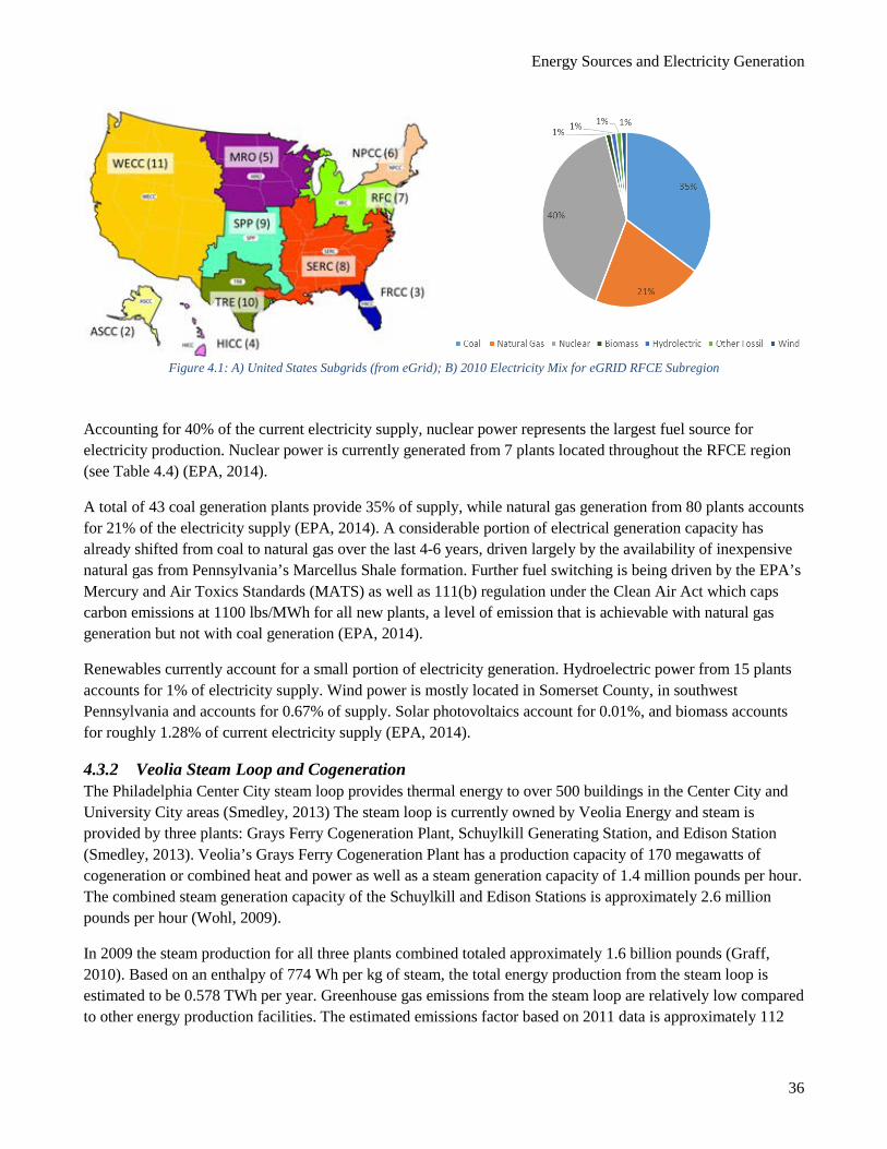
Energy Sources and Electricity Generation

36

Figure 4.1: A) United States Subgrids (from eGrid); B) 2010 Electricity Mix for eGRID RFCE Subregion

Accounting for 40% of the current electricity supply, nuclear power represents the largest fuel source for electricity production. Nuclear power is currently generated from 7 plants located throughout the RFCE region (see Table 4.4) (EPA, 2014).

A total of 43 coal generation plants provide 35% of supply, while natural gas generation from 80 plants accounts for 21% of the electricity supply (EPA, 2014). A considerable portion of electrical generation capacity has already shifted from coal to natural gas over the last 4-6 years, driven largely by the availability of inexpensive natural gas from Pennsylvania’s Marcellus Shale formation. Further fuel switching is being driven by the EPA’s Mercury and Air Toxics Standards (MATS) as well as 111(b) regulation under the Clean Air Act which caps carbon emissions at 1100 lbs/MWh for all new plants, a level of emission that is achievable with natural gas generation but not with coal generation (EPA, 2014).

Renewables currently account for a small portion of electricity generation. Hydroelectric power from 15 plants accounts for 1% of electricity supply. Wind power is mostly located in Somerset County, in southwest Pennsylvania and accounts for 0.67% of supply. Solar photovoltaics account for 0.01%, and biomass accounts for roughly 1.28% of current electricity supply (EPA, 2014).

4.3.2 Veolia Steam Loop and Cogeneration The Philadelphia Center City steam loop provides thermal energy to over 500 buildings in the Center City and University City areas (Smedley, 2013) The steam loop is currently owned by Veolia Energy and steam is provided by three plants: Grays Ferry Cogeneration Plant, Schuylkill Generating Station, and Edison Station (Smedley, 2013). Veolia’s Grays Ferry Cogeneration Plant has a production capacity of 170 megawatts of cogeneration or combined heat and power as well as a steam generation capacity of 1.4 million pounds per hour. The combined steam generation capacity of the Schuylkill and Edison Stations is approximately 2.6 million pounds per hour (Wohl, 2009).

In 2009 the steam production for all three plants combined totaled approximately 1.6 billion pounds (Graff, 2010). Based on an enthalpy of 774 Wh per kg of steam, the total energy production from the steam loop is estimated to be 0.578 TWh per year. Greenhouse gas emissions from the steam loop are relatively low compared to other energy production facilities. The estimated emissions factor based on 2011 data is approximately 112

Energy Sources and Electricity Generation

37

pounds eCO2 per MMBtu (Graff, 2010). Based on the emissions factor and the total steam generation data, a total of 104,531 tons eCO2 was emitted in 2010 from the steam loop system operation (Graff, 2010), corresponding to about 1% of the total Scope 2 emissions.

4.3.3 Local Generation In 2013, 5.1 GWh of renewable energy was generated within the City of Philadelphia by a combination of small, mostly private solar photovoltaic projects and larger institutional projects (Mayor's Office of Sustainability, 2013c). In the public sector, the Philadelphia Water department (PWD) operates a 5.6 MW biogas cogeneration project at the Northeast Water Pollution Control Plant and a 250KW solar PV plant at the Southeast Pollution Control Plant (Mayor's Office of Sustainability, 2013c). While there are currently no utility-scale PV plants within the city limits, several projects ranging from 1 to 6 MW’s have been built in the greater Philadelphia area with the support of Power Purchase Agreements (PPA’s) signed by off-takers within the city including universities and professional sports teams (Solar Energy Industries Association, 2014).

4.4 Assessment of Individual Fuel Emissions

4.4.1 Methodology Argonne National Laboratory’s GREET fuel cycle model was used to determine the lifecycle emissions for various electric grid mixes, including the 2010 baseline RFCE mix. Greenhouse gas emissions from each energy source are calculated as the total emissions starting with the collection and transportation of the feedstock to the operation of the generation plant. Fuel cycle emissions are calculated in GREET using emissions factors from the Energy Information Administration (EIA) for electricity generation from residual oil, coal, natural gas, biomass, nuclear, and renewables, which includes hydroelectric, geothermal, wind, and solar PV. All greenhouse gas emissions are expressed in terms of CO2e per kWh of energy produced. Emissions for coal and natural gas power generation are calculated with the assumption of no carbon capture and sequestration.

4.4.2 Current Emissions and sensitivity to fuel changes Through GREET, it was possible to determine the sensitivity of emissions to changes in fuel sources, that is, the change in emissions that would occur when a unit of energy (i.e. 1 kWh) is produced with one fuel rather than another. This sensitivity analysis is aimed at estimating the emissions tradeoffs between fuel sources and aid the identification of future mix scenarios compatible with target reductions.

The analysis considered switching energy sources to and from natural gas, coal, nuclear, biomass, and renewables. For this analysis renewables include solar, wind, geothermal, and hydroelectric energy sources. The renewable energy sources were grouped together as GREET designates all electricity production from these sources as having zero upstream and in use carbon emissions.

The results of the sensitivity analysis are summarized in Table 4.1. Negative values indicate a decrease in greenhouse gas emissions whereas positive values indicate an increase. Results are shown in units of grams CO2e per kWh of energy produced by each respective source. This analysis indicates that most greenhouse gas emissions savings would come from adopting alternative energy sources in lieu of coal. More specifically, the greatest savings would be achieved by switching from coal to either renewables or nuclear power. From these sensitivities, it is possible to determine which electric grid mixes could be used in the future to achieve target reductions.

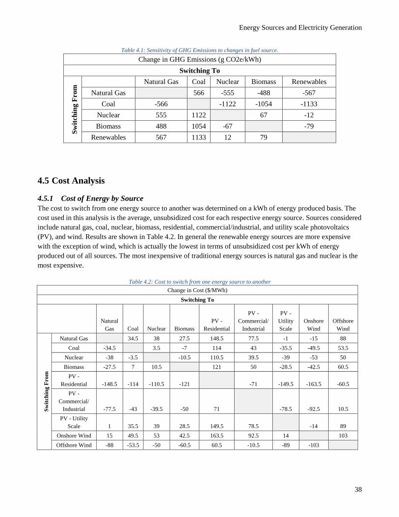
Energy Sources and Electricity Generation

38

Table 4.1: Sensitivity of GHG Emissions to changes in fuel source. Change in GHG Emissions (g CO2e/kWh)

Switching To Sw

itchi

ng F

rom

Natural Gas Coal Nuclear Biomass Renewables Natural Gas 566 -555 -488 -567

Coal -566 -1122 -1054 -1133 Nuclear 555 1122 67 -12 Biomass 488 1054 -67 -79

Renewables 567 1133 12 79

4.5 Cost Analysis

4.5.1 Cost of Energy by Source The cost to switch from one energy source to another was determined on a kWh of energy produced basis. The cost used in this analysis is the average, unsubsidized cost for each respective energy source. Sources considered include natural gas, coal, nuclear, biomass, residential, commercial/industrial, and utility scale photovoltaics (PV), and wind. Results are shown in Table 4.2. In general the renewable energy sources are more expensive with the exception of wind, which is actually the lowest in terms of unsubsidized cost per kWh of energy produced out of all sources. The most inexpensive of traditional energy sources is natural gas and nuclear is the most expensive.

Table 4.2: Cost to switch from one energy source to another Change in Cost ($/MWh)

Switching To

Natural

Gas Coal Nuclear Biomass PV -

Residential

PV - Commercial/

Industrial

PV - Utility Scale

Onshore Wind

Offshore Wind

Switc

hing

Fro

m

Natural Gas 34.5 38 27.5 148.5 77.5 -1 -15 88 Coal -34.5 3.5 -7 114 43 -35.5 -49.5 53.5

Nuclear -38 -3.5 -10.5 110.5 39.5 -39 -53 50 Biomass -27.5 7 10.5 121 50 -28.5 -42.5 60.5

PV - Residential -148.5 -114 -110.5 -121 -71 -149.5 -163.5 -60.5

PV - Commercial/

Industrial -77.5 -43 -39.5 -50 71 -78.5 -92.5 10.5 PV - Utility

Scale 1 35.5 39 28.5 149.5 78.5 -14 89 Onshore Wind 15 49.5 53 42.5 163.5 92.5 14 103 Offshore Wind -88 -53.5 -50 -60.5 60.5 -10.5 -89 -103

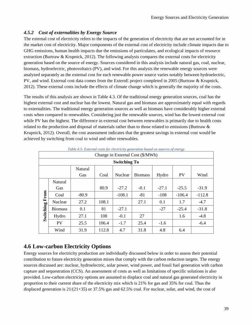
Energy Sources and Electricity Generation

39

4.5.2 Cost of externalities by Energy Source The external cost of electricity refers to the impacts of the generation of electricity that are not accounted for in the market cost of electricity. Major components of the external cost of electricity include climate impacts due to GHG emissions, human health impacts due the emissions of particulates, and ecological impacts of resource extraction (Burtraw & Krupnick, 2012). The following analysis compares the external costs for electricity generation based on the source of energy. Sources considered in this analysis include natural gas, coal, nuclear, biomass, hydroelectric, photovoltaics (PV), and wind. For this analysis the renewable energy sources were analyzed separately as the external cost for each renewable power source varies notably between hydroelectric, PV, and wind. External cost data comes from the ExternE project completed in 2005 (Burtraw & Krupnick, 2012). These external costs include the effects of climate change which is generally the majority of the costs.

The results of this analysis are shown in Table 4.3. Of the traditional energy generation sources, coal has the highest external cost and nuclear has the lowest. Natural gas and biomass are approximately equal with regards to externalities. The traditional energy generation sources as well as biomass have considerably higher external costs when compared to renewables. Considering just the renewable sources, wind has the lowest external cost while PV has the highest. The difference in external cost between renewables is primarily due to health costs related to the production and disposal of materials rather than to those related to emissions (Burtraw & Krupnick, 2012). Overall, the cost assessment indicates that the greatest savings in external cost would be achieved by switching from coal to wind and other renewables.

Table 4.3: External costs for electricity generation based on sources of energy Change in External Cost ($/MWh)

Switching To

Natural

Gas Coal Nuclear Biomass Hydro PV Wind

Switc

hing

Fro

m

Natural Gas 80.9 -27.2 -0.1 -27.1 -25.5 -31.9 Coal -80.9 -108.1 -81 -108 -106.4 -112.8

Nuclear 27.2 108.1 27.1 0.1 1.7 -4.7 Biomass 0.1 81 -27.1 -27 -25.4 -31.8 Hydro 27.1 108 -0.1 27 1.6 -4.8

PV 25.5 106.4 -1.7 25.4 -1.6 -6.4 Wind 31.9 112.8 4.7 31.8 4.8 6.4

4.6 Low-carbon Electricity Options Energy sources for electricity production are individually discussed below in order to assess their potential contribution to future electricity generation mixes that comply with the carbon reduction targets. The energy sources discussed are: nuclear, hydroelectric, solar power, wind power, and fossil fuel generation with carbon capture and sequestration (CCS). An assessment of costs as well as limitations of specific solutions is also provided. Low-carbon electricity options are assumed to displace coal and natural gas generated electricity in proportion to their current share of the electricity mix which is 21% for gas and 35% for coal. Thus the displaced generation is 21/(21+35) or 37.5% gas and 62.5% coal. For nuclear, solar, and wind, the cost of

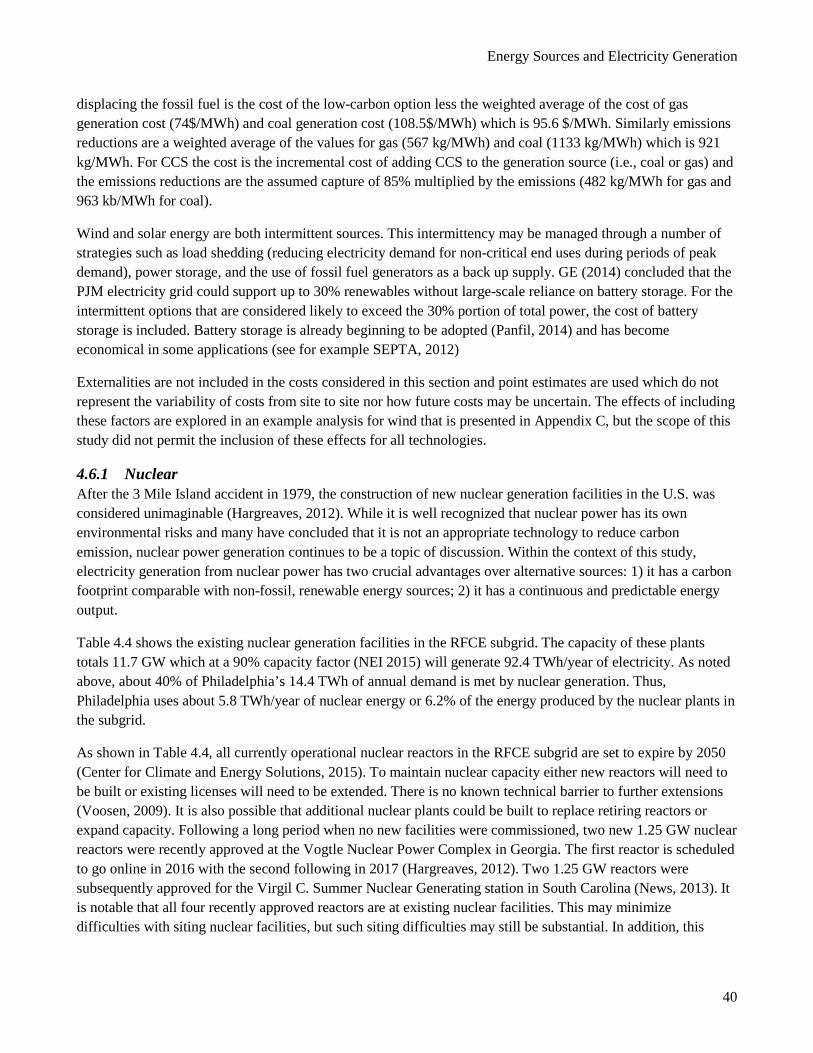
Energy Sources and Electricity Generation

40

displacing the fossil fuel is the cost of the low-carbon option less the weighted average of the cost of gas generation cost (74$/MWh) and coal generation cost (108.5$/MWh) which is 95.6 $/MWh. Similarly emissions reductions are a weighted average of the values for gas (567 kg/MWh) and coal (1133 kg/MWh) which is 921 kg/MWh. For CCS the cost is the incremental cost of adding CCS to the generation source (i.e., coal or gas) and the emissions reductions are the assumed capture of 85% multiplied by the emissions (482 kg/MWh for gas and 963 kb/MWh for coal).

Wind and solar energy are both intermittent sources. This intermittency may be managed through a number of strategies such as load shedding (reducing electricity demand for non-critical end uses during periods of peak demand), power storage, and the use of fossil fuel generators as a back up supply. GE (2014) concluded that the PJM electricity grid could support up to 30% renewables without large-scale reliance on battery storage. For the intermittent options that are considered likely to exceed the 30% portion of total power, the cost of battery storage is included. Battery storage is already beginning to be adopted (Panfil, 2014) and has become economical in some applications (see for example SEPTA, 2012)

Externalities are not included in the costs considered in this section and point estimates are used which do not represent the variability of costs from site to site nor how future costs may be uncertain. The effects of including these factors are explored in an example analysis for wind that is presented in Appendix C, but the scope of this study did not permit the inclusion of these effects for all technologies.

4.6.1 Nuclear After the 3 Mile Island accident in 1979, the construction of new nuclear generation facilities in the U.S. was considered unimaginable (Hargreaves, 2012). While it is well recognized that nuclear power has its own environmental risks and many have concluded that it is not an appropriate technology to reduce carbon emission, nuclear power generation continues to be a topic of discussion. Within the context of this study, electricity generation from nuclear power has two crucial advantages over alternative sources: 1) it has a carbon footprint comparable with non-fossil, renewable energy sources; 2) it has a continuous and predictable energy output.

Table 4.4 shows the existing nuclear generation facilities in the RFCE subgrid. The capacity of these plants totals 11.7 GW which at a 90% capacity factor (NEI 2015) will generate 92.4 TWh/year of electricity. As noted above, about 40% of Philadelphia’s 14.4 TWh of annual demand is met by nuclear generation. Thus, Philadelphia uses about 5.8 TWh/year of nuclear energy or 6.2% of the energy produced by the nuclear plants in the subgrid.

As shown in Table 4.4, all currently operational nuclear reactors in the RFCE subgrid are set to expire by 2050 (Center for Climate and Energy Solutions, 2015). To maintain nuclear capacity either new reactors will need to be built or existing licenses will need to be extended. There is no known technical barrier to further extensions (Voosen, 2009). It is also possible that additional nuclear plants could be built to replace retiring reactors or expand capacity. Following a long period when no new facilities were commissioned, two new 1.25 GW nuclear reactors were recently approved at the Vogtle Nuclear Power Complex in Georgia. The first reactor is scheduled to go online in 2016 with the second following in 2017 (Hargreaves, 2012). Two 1.25 GW reactors were subsequently approved for the Virgil C. Summer Nuclear Generating station in South Carolina (News, 2013). It is notable that all four recently approved reactors are at existing nuclear facilities. This may minimize difficulties with siting nuclear facilities, but such siting difficulties may still be substantial. In addition, this

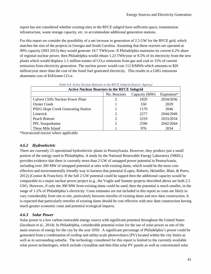
Energy Sources and Electricity Generation

41

report has not considered whether existing sites in the RFCE subgrid have sufficient space, transmission infrastructure, waste storage capacity, etc. to accommodate additional generation stations.

For this report we consider the possibility of a net increase in generation of 2.5 GW for the RFCE grid, which matches the size of the projects in Georgia and South Carolina. Assuming that these reactors are operated at 90% capacity (NEI 2015) they would generate 19.7 TWh/year. If Philadelphia maintains its current 6.2% share of regional nuclear power, then Philadelphia would obtain 1.23 TWh/year or 8.5% of its electricity from the new plants which would displace 1.1 million tonnes of CO2e emissions from gas and coal or 15% of current emissions from electricity generation. The nuclear power would cost 112 $/MWh which amounts to $20 million/year more than the cost of the fossil fuel generated electricity. This results in a GHG emissions abatement cost of $18/tonne CO2e.

Table 4.4: Active Nuclear Reactors in the RFCE Subgrid (Source: Agency) Active Nuclear Reactors in the RFCE Subgrid

No. Reactors Capacity (MW) Expiration* Calvert Cliffs Nuclear Power Plant 2 1829 2034/2036 Oyster Creek 1 550 2029 PSEG Hope Creek Generating Station 1 1170 2046 Limerick 2 2277 2044/2049 Peach Bottom 2 2319 2033/2034 PPL Susquehanna 2 2596 2042/2044 Three Mile Island 1 976 2034

*first/second reactor where applicable

4.6.2 Hydroelectric There are currently 15 operational hydroelectric plants in Pennsylvania. However, they produce just a small portion of the energy used in Philadelphia. A study by the National Renewable Energy Laboratory (NREL) provides evidence that there is currently more than 2 GW of untapped power potential in Pennsylvania, including over 300 MW of untapped potential at sites with existing dams, which would be the most cost-effective and environmentally friendly way to harness that potential (Lopez, Roberts, Heimiller, Blair, & Porro, 2012) (Connor & Francfort). If the full 2 GW potential could be tapped then the additional capacity would be comparable to a major nuclear power project (e.g., the Vogtle and Sumner projects described above are both 2.5 GW). However, if only the 300 MW from existing dams could be used, then the potential is much smaller, in the range of 1-2% of Philadelphia’s electricity. Costs estimates are not included in this report as costs are likely to vary considerably from site to site, particularly between retrofits of existing dams and new dam construction. It is expected that particularly retrofits of existing dams should be cost effective with new dam construction having much greater economic costs and potential ecological impacts.

4.6.3 Solar Power Solar power is a low carbon renewable energy source with significant potential throughout the United States (Jacobson et al., 2014). In Philadelphia, considerable potential exists for the use of solar power as one of the main sources of energy for the city by the year 2050. A significant percentage of Philadelphia’s power could be generated from a combination of rooftop and utility-scale photovoltaics (PV) located within the city limits as well as in surrounding suburbs. The technology considered for this report is limited to the currently available solar power technologies, which include crystalline and thin-film solar PV panels as well as concentrated solar

Energy Sources and Electricity Generation

42

power (CSR). The National Renewable Energy Laboratory (NREL) provided estimates of the annual average solar resource potential, based on the Climatological Solar Radiation Model, which takes into account seasonal variations in cloud cover and atmospheric conditions, such as concentration of trace gases and aerosols (Roberts, 2012). NREL estimates that the CSR resource potential for Philadelphia and its surrounding counties is less than 5 kWh/m2/day, which is below the threshold recommended for CSR implementation. Therefore, CSR technology is not considered to be viable for electricity generation in Philadelphia and its suburbs. Both crystalline and thin-film PV panels are considered feasible for this region (Lopez et al., 2012).

Given the potential for both rooftop and utility scale photovoltaic in the region, solar energy will represent a significant component in the future energy mix developed in this report. In fact, the technical potential for solar energy in the area served by the RFCE grid would be theoretically sufficient to power the entire grid. However, technical limitations (e.g. a power grid cannot rely solely on intermittent renewable energy sources) and political and socio-economic obstacles suggest using a mix of electricity generation sources. Accordingly the extent of solar power development considered in this report is ambitious but still well below the physical potential of the resource. Five different options for solar photovoltaics are considered: residential rooftops, commercial and industrial rooftops, vacant land in Philadelphia, utility scale without storage in surrounding counties, and utility scale with storage in surrounding counties. The potential of each of these options is describe below with results summarized in Table 4.5.

4.6.3.1 Rooftop Photovoltaics The following analysis provides an estimate for the potential annual energy generation from rooftop PV located within Philadelphia’s city limits. An average solar resource potential of 4.75 kWh/m2/day was used for the calculations.

Geographic Information System (GIS) datasets from 2004 and 2011 were used to estimate the rooftop area available in Philadelphia for solar power systems installation. Both datasets were obtained from the Pennsylvania Spatial Data Clearinghouse (PASDA). The first dataset from 2004 was developed by the Philadelphia Water Department (PWD) and is a planimetric coverage of building footprints in Philadelphia ("Pennsylvania Spatial Data Access ", 2015). The second dataset is polygon coverage depicting land use by parcel in Philadelphia. The land use dataset is from 2011 and was developed by the City of Philadelphia ("Pennsylvania Spatial Data Access ", 2015).

Equation 4.1 was used to calculate the total annual energy generation for rooftop PV:

P = A * E * L * 4.75 kWh/m2-day * 365 days/year * 10-9 (4.1)

where P is the total annual energy generation in TWh, A is total rooftop area available for PV in m2, E is average efficiency of the solar panel modules, and L is the estimated average DC-to-AC conversion factor.

Given that conversion factors, as well as the fraction of usable rooftop surface, differ between residential and commercial/industrial rooftop systems, separate estimates were developed for residential and commercial/industrial PV systems. Another key assumption of this analysis is that building growth or turnover between 2004 and 2050 would not be significant enough to substantially alter the results.

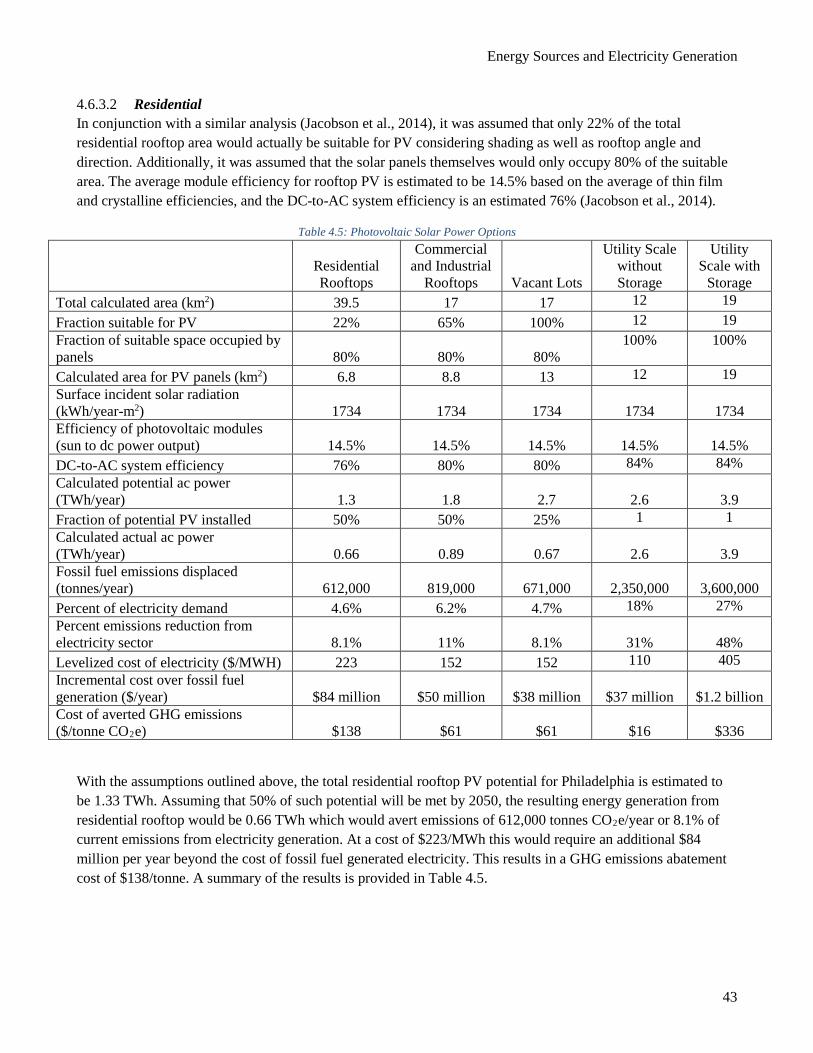
Energy Sources and Electricity Generation

43

4.6.3.2 Residential In conjunction with a similar analysis (Jacobson et al., 2014), it was assumed that only 22% of the total residential rooftop area would actually be suitable for PV considering shading as well as rooftop angle and direction. Additionally, it was assumed that the solar panels themselves would only occupy 80% of the suitable area. The average module efficiency for rooftop PV is estimated to be 14.5% based on the average of thin film and crystalline efficiencies, and the DC-to-AC system efficiency is an estimated 76% (Jacobson et al., 2014).

Table 4.5: Photovoltaic Solar Power Options

With the assumptions outlined above, the total residential rooftop PV potential for Philadelphia is estimated to be 1.33 TWh. Assuming that 50% of such potential will be met by 2050, the resulting energy generation from residential rooftop would be 0.66 TWh which would avert emissions of 612,000 tonnes CO2e/year or 8.1% of current emissions from electricity generation. At a cost of $223/MWh this would require an additional $84 million per year beyond the cost of fossil fuel generated electricity. This results in a GHG emissions abatement cost of $138/tonne. A summary of the results is provided in Table 4.5.

Residential Rooftops

Commercial and Industrial

Rooftops Vacant Lots

Utility Scale without Storage

Utility Scale with

Storage Total calculated area (km2) 39.5 17 17 12 19 Fraction suitable for PV 22% 65% 100% 12 19 Fraction of suitable space occupied by panels 80% 80% 80%

100% 100%

Calculated area for PV panels (km2) 6.8 8.8 13 12 19 Surface incident solar radiation (kWh/year-m2) 1734 1734 1734

1734

1734

Efficiency of photovoltaic modules (sun to dc power output) 14.5% 14.5% 14.5%

14.5%

14.5%

DC-to-AC system efficiency 76% 80% 80% 84% 84% Calculated potential ac power (TWh/year) 1.3 1.8 2.7

2.6

3.9

Fraction of potential PV installed 50% 50% 25% 1 1 Calculated actual ac power (TWh/year) 0.66 0.89 0.67

2.6

3.9

Fossil fuel emissions displaced (tonnes/year) 612,000 819,000 671,000

2,350,000

3,600,000

Percent of electricity demand 4.6% 6.2% 4.7% 18% 27% Percent emissions reduction from electricity sector 8.1% 11% 8.1%

31%

48%

Levelized cost of electricity ($/MWH) 223 152 152 110 405 Incremental cost over fossil fuel generation ($/year) $84 million $50 million $38 million

$37 million

$1.2 billion

Cost of averted GHG emissions ($/tonne CO2e) $138 $61 $61

$16

$336

Energy Sources and Electricity Generation

44

4.6.3.3 Commercial/Industrial In the case of commercial/industrial rooftop area, it was assumed that 65% of the total area would be suitable for PV. Again, it was assumed that only 80% of the suitable area would be occupied by solar panels. The average module efficiency is again 14.5%. The estimated DC-to-AC system efficiency for commercial/industrial module set-ups is 80% (Jacobson et al., 2014).

The total potential estimated for commercial/industrial rooftop PV in Philadelphia is approximately 1.7 TWh. Assuming again that PV will be installed on 50% of the available area, the resulting energy generation comes to 0.84 TWh which would avert emissions of 819,000 tonnes CO2e/year or 11% of current emissions from electricity generation. At a cost of $152/MWh this would require an additional $50 million per year beyond the cost of fossil fuel generated electricity. This results in a GHG emissions abatement cost of $61/tonne. A summary of the results is provided in Table 4.5.

4.6.3.4 Photovoltaics on urban vacant land Philadelphia has a considerable amount of vacant land that might be used for the photovoltaic power generation. Many such small lots would offer economies of scale similar to residential photovoltaics, which are not particularly favorable (abatement cost of $130/tonne as described above). For this reason only lots of at least 18,000 m2 (134 m x 134m) were considered here. These lots were considered of sufficient size to achieve the economies of scale associated with the commercial and industrial application, but not with utility-scale applications. GIS was used to estimate the total area of vacant lots having a contiguous surface of at least 18,000 m2 in Philadelphia as 16.7 km2. All undeveloped, empty lots in the city were considered to be vacant. The area does not include lots with unoccupied or abandoned buildings nor does it include lots that are used for recreational purposes.

Equation 1 was used to estimate the annual power generation. It was assumed that all vacant lot area would be suitable for PV, but again only 80% of the area would actually be occupied with panels. The average module efficiency for the panels is the same as the module efficiency for rooftop PV. DC-to-AC conversion system efficiency is estimated to be 84% for utility-scale module arrangements (Jacobson et al., 2014).

If utility-scale PV plants were installed on all vacant lots in Philadelphia the annual power generation potential would be approximately 2.82 TWh. It is recognized that this scenario is extremely unlikely so it was estimated that only 25% of the available vacant lots would be developed into PV plants giving a generation potential of 0.70 TWh. which would avert emissions of 671,000 tonnes CO2e/year or 8.1% of current emissions from electricity generation. At a cost of $152/MWh (it is assumed that economies of scale are similar to commercial and industrial rooftop applications) this would require an additional $38 million per year beyond the cost of fossil fuel generated electricity. This results in a GHG emissions abatement cost of $61/tonne. Note that these costs do not account for additional land acquirement costs that might apply in an urban setting. A summary of the results can be seen in Table 4.5.

4.6.3.5 Utility-scale Photovoltaics Utility-scale PV offers considerable economies of scale over rooftop PV applications. As a conservative measure, these more favorable economics were not applied to PV within the city limits but it was considered feasible to achieve implement larger scale PV generation in the surrounding counties. A total of 6.5 TWh/year was set which would provide for 45% of Philadelphia’s current electricity demand. To assess whether the land

Energy Sources and Electricity Generation

45

requirements would be feasible, Equation 4.1 above was manipulated so that the amount of land area could be calculated relative to a known amount of power generation. Approximately 38.5 km2 of rural open land would be required to generate 6.50 TWh through the use of utility-scale PV. This amounts to approximately 1.2% of the total land area of Delaware, Montgomery, and Bucks counties, an amount that was considered feasible.

The provision of 6.5 TWh/year from solar power would substantially exceed the 30% of electricity that can be supplied by intermittent sources without the use of storage (GE 2014). Thus, there are two distinct costs associated with utility-scale PV. The first cost is for provision as an intermittent source and is applicable to the portion of utility scale generation that fits within the 30% limit for intermittent sources. It was assumed that onshore wind (described below) would account for 6.1% of electricity demand and commercial rooftop PV (described above) would account for 6.2% of electricity demand. Minimal adoption of residential PV was assumed given its less favorable economics compared to commercial rooftop PV. Minimal use of vacant lots in Philadelphia was assumed, although any that is developed could be substituted for either commercial rooftop (at small sites where economies of scale are limited) or utility scale (if the sites in the city are large enough then land in the city could be used rather than land in surrounding counties). Subtracting the onshore wind and commercial rooftop PV from the 30% available for intermittent power sources left 17.7% of current demand or 2.6 TWh/year that could be supplied by utility scale solar without the use of storage. This amount of solar power would avert emissions of 2,350,000 tonnes CO2e/year or 31% of current emissions from electricity generation. Lazard (2014) indicates that the average LCOE for utility-scale solar is 79 $/MWh which is less than the cost of fossil fuel generation. However, many current utility-scale generation facilities are in areas with low land costs and high solar radiation. Germany has extensively developed solar power despite modest insolation rates. Kost et al. (2013) found that utility scale PV in Germany had a LCOE of roughly 0.08 to 0.115 Euros per kWh. The midpoint of this range, 0.0975, equates to 0.11 $/kWh or 110$/MWh at an exchange rate of 1 Euro=$1.12. This is a marginal cost of 14$/kWh compared to fossil fuel generation which amounts to an additional $37 million per year beyond the cost of fossil fuel generated electricity. This results in a GHG emissions abatement cost of $16/tonne.

Of the total 6.5 TWh/year of utility scale solar, the remaining 3.9 TWh/year is assumed to require battery storage. This 3.9 TWh/year would avert emissions of 3.6 million tonnes/year of CO2e.or 48% of current emissions from electricity generation. The storage adds 295 $/MWh to the cost for a marginal cost of 309 $/MWh which amounts to $1.2 billion beyond the cost of fossil fuel generated electricity. This results in a GHG emissions abatement cost of $336/tonne. Lazard (2014) forecasts that batter storage costs may decline by 40% by 2017 which would reduce the abatement cost to $208/tonne. A summary of the results is provided in Table 4.5.

4.6.4 Wind Power Wind power is a relatively inexpensive, carbon-free means of energy production with significant onshore potential in Pennsylvania and offshore potential on the east coast of the United States. As in the case of solar power, while the combined onshore and offshore wind potential would exceed Philadelphia’s 2050 demand for electricity, given the uncertainties in future policy and in the interest of providing a balance between future energy sources, the fraction of such potential that could reasonably be exploited is likely much lower. As with solar, the extent of wind development considered is ambitious but well below the physical potential of the resource. On-shore and off-shore options are discussed below with results summarized in Table 4.6.

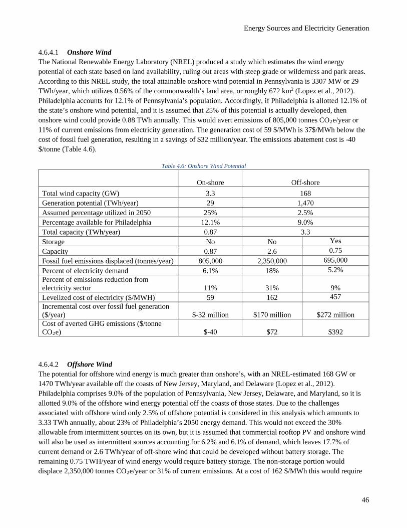
Energy Sources and Electricity Generation

46

4.6.4.1 Onshore Wind The National Renewable Energy Laboratory (NREL) produced a study which estimates the wind energy potential of each state based on land availability, ruling out areas with steep grade or wilderness and park areas. According to this NREL study, the total attainable onshore wind potential in Pennsylvania is 3307 MW or 29 TWh/year, which utilizes 0.56% of the commonwealth’s land area, or roughly 672 km2 (Lopez et al., 2012). Philadelphia accounts for 12.1% of Pennsylvania’s population. Accordingly, if Philadelphia is allotted 12.1% of the state’s onshore wind potential, and it is assumed that 25% of this potential is actually developed, then onshore wind could provide 0.88 TWh annually. This would avert emissions of 805,000 tonnes CO2e/year or 11% of current emissions from electricity generation. The generation cost of 59 $/MWh is 37$/MWh below the cost of fossil fuel generation, resulting in a savings of $32 million/year. The emissions abatement cost is -40 $/tonne (Table 4.6).

Table 4.6: Onshore Wind Potential

On-shore

Off-shore Total wind capacity (GW) 3.3 168 Generation potential (TWh/year) 29 1,470 Assumed percentage utilized in 2050 25% 2.5% Percentage available for Philadelphia 12.1% 9.0% Total capacity (TWh/year) 0.87 3.3 Storage No No Yes Capacity 0.87 2.6 0.75 Fossil fuel emissions displaced (tonnes/year) 805,000 2,350,000 695,000 Percent of electricity demand 6.1% 18% 5.2% Percent of emissions reduction from electricity sector 11% 31%

9%

Levelized cost of electricity ($/MWH) 59 162 457 Incremental cost over fossil fuel generation ($/year) $-32 million $170 million

$272 million

Cost of averted GHG emissions ($/tonne CO2e) $-40 $72

$392

4.6.4.2 Offshore Wind The potential for offshore wind energy is much greater than onshore’s, with an NREL-estimated 168 GW or 1470 TWh/year available off the coasts of New Jersey, Maryland, and Delaware (Lopez et al., 2012). Philadelphia comprises 9.0% of the population of Pennsylvania, New Jersey, Delaware, and Maryland, so it is allotted 9.0% of the offshore wind energy potential off the coasts of those states. Due to the challenges associated with offshore wind only 2.5% of offshore potential is considered in this analysis which amounts to 3.33 TWh annually, about 23% of Philadelphia’s 2050 energy demand. This would not exceed the 30% allowable from intermittent sources on its own, but it is assumed that commercial rooftop PV and onshore wind will also be used as intermittent sources accounting for 6.2% and 6.1% of demand, which leaves 17.7% of current demand or 2.6 TWh/year of off-shore wind that could be developed without battery storage. The remaining 0.75 TWH/year of wind energy would require battery storage. The non-storage portion would displace 2,350,000 tonnes CO2e/year or 31% of current emissions. At a cost of 162 $/MWh this would require

Energy Sources and Electricity Generation

47

an additional $170 million per year beyond the cost of fossil fuel generated electricity which results in a GHG abatement cost of $72/tonne. The portion requiring storage would displace 695,000 tonnes CO2e/year or 9% of emissions from electricity generation. At a cost of 457 $/MWh this would require $170 million per year above the cost of fossil fuel generated electricity, which results in a GHG abatement cost of $392/tonne.

4.6.5 Carbon Capture and Sequestration Carbon capture and sequestration (CCS) involves using conventional fossil fuels (coal and natural gas) to generate electricity but avoiding the release of the CO2 into the atmosphere. The process is inherently less energetically efficient than atmospheric release of CO2 as additional energy is needed to separate the CO2 from other flue gases, to transport the CO2 to a reservoir, and to inject the CO2 into the reservoir. In the absence of hard constraints on carbon emissions the process is not economically favored, and there have been only limited applications of the technology. Current estimates for carbon capture from power production range from $60 to $114 per ton of CO2 avoided, largely based on type of power plant ("Report of the Interagency Task Force on Carbon Capture and Storage," 2013).

4.6.5.1 Carbon Capture Various commercially available CCS technologies are currently being utilized in the power generation industry both nationally and internationally ("Phase II Final Report," 2011) ("Report of the Interagency Task Force on Carbon Capture and Storage," 2013). CCS technologies are typically geared towards pulverized coal (PC), integrated coal gasification combined cycle (IGCC), or natural gas (NG) plants ("Report of the Interagency Task Force on Carbon Capture and Storage," 2013). Carbon can be captured either pre- or post-combustion, or through a process known as oxy-combustion ("Report of the Interagency Task Force on Carbon Capture and Storage," 2013). Regardless of the technology used, typical capture efficiencies are around 90% of carbon produced (2013).

Pre-combustion is generally only applicable to IGCC, where the coal is converted to gaseous components (“syngas”). The cost of electricity (COE) from IGCC is higher than from PC, which, based on a review of the eGRID energy database, is assumed to be the only operational coal source within Philadelphia’s energy grid ("eGRID 9th Edition Version 1.0," 2014). COE is expected to increase by 40% at an IGCC plant implementing CCS technology. An IGCC plant implementing CCS technology would experience an energy penalty of 20% due to the energy necessary to capture and compress 90% of the carbon produced. The energy demands and losses inherent in these process changes would result in a 40% increase in COE ("Report of the Interagency Task Force on Carbon Capture and Storage," 2013). This stands in contrast to a PC plant, where COE is expected to rise by nearly 80% with the addition of a post-combustion amine scrubber for carbon capture, and would result in an energy penalty close to 30% ("Report of the Interagency Task Force on Carbon Capture and Storage," 2013).

Oxy-combustion is a relatively new technology that combusts the fuel in a stream of purified O2 mixed with recycled CO2. Oxy-combustion comes with some important technical and economic advantages that ultimately reduce both carbon capture cost and emission of other criteria pollutants such as NOx, SOx, and Hg. An oxy-combustion coal-fired power plant equipped for carbon capture would increase COE by about 60% at an energy penalty of roughly 25% compared to a similar plant without carbon capture technology ("Report of the Interagency Task Force on Carbon Capture and Storage," 2013).

Energy Sources and Electricity Generation

48

4.6.5.2 Existing Applications Globally, carbon capture and geologic sequestration has been demonstrated at the commercial scale at four primary locations: Sleipner in the North Sea, Snøhvit in the Barents Sea, In Salah in Algeria, and Weyburn in Canada ("Phase II Final Report," 2011) ("Report of the Interagency Task Force on Carbon Capture and Storage," 2013). Combined, these four projects represent over 25 years of carbon capture and geologic storage experience. A coal-fired power plant with carbon capture technology is under construction in Kemper County Mississippi and is expected to be fully operational in 2016 (Kemper Project, 2016). Proponents note that this is among the most cost-effective ways to reduce atmospheric emissions while others raise concerns over risks of transporting CO2 and potential for release from geologic reservoirs in the long term or even in the shorter term (Richard, 2006).

4.6.5.3 Carbon Storage Potential Carbon dioxide can be sequestered over relatively long periods either geologically or terrestrially. Geologic surveys of the Midwest region (stretching from Kentucky to New York) indicate that there is capacity to permanently contain hundreds of years of CO2 emissions from the region. Pennsylvania alone is estimated to house approximately 33.7 billion metric tons of geologic storage space ("Phase II Final Report," 2011). Deep saline formations provide the commonwealth’s largest storage capacity at 30.1 billion metric tons, while the remainder comes from depleted oil and gas reservoirs, organic shale layers, and coalbeds ("Phase II Final Report," 2011). At Philadelphia’s current average electricity consumption of 14.4 TWh/year which produces 7.6 million tonnes CO2e , Pennsylvania’s geologic carbon storage capacity would last approximately 478 years given that Philadelphia’s population represents about 12.5% of the state’s total and assuming that a proportional amount of storage would be allocated for carbon storage ("eGRID 9th Edition Version 1.0," 2014).

Enhanced oil recovery (EOR) is the engineered injection of CO2 into a producing oil or gas well in order to improve the overall production efficiency. This process re-pressurizes the reservoir, which increases the mobility of the fuel reserves held within while also providing an economic incentive for CCS deployment. As CO2 is currently in limited supply for these operations, increased CO2 capture would lower the barriers to effective implementation of EOR ("Report of the Interagency Task Force on Carbon Capture and Storage," 2013). Pennsylvania’s EOR storage capacity is estimated at 2.8 billion metric tons ("Phase II Final Report," 2011) or 45 years of emissions from electricity supply for Philadelphia.

Coalbed methane is locally captured from more than 24 sources in Pennsylvania. These gassy coal deposits, in combination with so-called ‘unmineable’ coal seams, provide the potential for additional carbon storage, while also generating economic incentive in the form of additional natural gas production ("Phase II Final Report," 2011) ("Report of the Interagency Task Force on Carbon Capture and Storage," 2013). Pennsylvania is estimated to contain 66 million tons of coalbed carbon storage ("Phase II Final Report," 2011), sufficient for 1.1 years of emissions from Philadelphia.

Pennsylvania has widespread regions containing thick layers of organic shale. Oftentimes, these shale layers can act as unconventional oil and gas reservoirs while also providing a seal for the underlying reservoirs. Similar to coalbed methane capture, CO2 injection could be used to enhance existing oil and gas production in these shales. In total, Pennsylvania is estimated to contain 726 million tons of shalebed carbon storage ("Phase II Final Report," 2011), sufficient for 12 years of emissions. Furthermore, laboratory testing indicates that these organic shales are expected to adsorb CO2, providing long term carbon sequestration potential. While laboratory testing

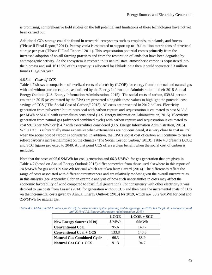
Energy Sources and Electricity Generation

49

is promising, comprehensive field studies on the full potential and limitations of these technologies have not yet been carried out.

Additional CO2 storage could be found in terrestrial ecosystems such as croplands, minelands, and forests ("Phase II Final Report," 2011). Pennsylvania is estimated to support up to 19.1 million metric tons of terrestrial storage per year ("Phase II Final Report," 2011). This sequestration potential comes primarily from the increased adoption of no-till farming practices and from the restoration of lands that have been degraded by anthropogenic activity. As the ecosystem is restored to its natural state, atmospheric carbon is sequestered into the biomass and soil. If 12.5% of this capacity is allocated for Philadelphia then it could sequester 2.3 million tonnes CO2e per year.

4.6.5.4 Costs of CCS Table 4.7 shows a comparison of levelized costs of electricity (LCOE) for energy from both coal and natural gas with and without carbon capture, as outlined by the Energy Information Administration in their 2015 Annual Energy Outlook (U.S. Energy Information Administration, 2015). The social costs of carbon, $39.81 per ton emitted in 2015 (as estimated by the EPA) are presented alongside these values to highlight the potential cost savings of CCS ("The Social Cost of Carbon," 2013). All costs are presented in 2012 dollars. Electricity generation from pulverized bituminous coal with carbon capture and sequestration is estimated to cost $133.8 per MWh or $140.6 with externalities considered (U.S. Energy Information Administration, 2015). Electricity generation from natural gas (advanced combined cycle) with carbon capture and sequestration is estimated to cost $91.3 per MWh or $94.7 with externalities considered (U.S. Energy Information Administration, 2015). While CCS is substantially more expensive when externalities are not considered, it is very close to cost neutral when the social cost of carbon is considered. In addition, the EPA’s social cost of carbon will continue to rise to reflect carbon’s increasing impact on the climate ("The Social Cost of Carbon," 2013). Table 4.8 presents LCOE and SCC figures projected to 2040. At that point CCS offers a clear benefit when the social cost of carbon is included.

Note that the costs of 95.6 $/MWh for coal generation and 66.3 $/MWh for gas generation that are given in Table 4.7 (based on Annual Energy Outlook 2015) differ somewhat from those used elsewhere in this report of 74 $/MWh for gas and 109 $/MWh for coal which are taken from Lazard (2014). The differences reflect the range of costs associated with different circumstances and are relatively modest given the overall uncertainties in this analysis (see Appendix C for an example analysis of how such uncertainties in costs may affect the economic favorability of wind compared to fossil fuel generation). For consistency with other electricity it was decided to use costs from Lazard (2014) for generation without CCS and then base the incremental costs of CCS on the incremental costs given by Annual Energy Outlook (2015) for 2019, which are 38.2 $/MWh for coal and 25$/MWh for natural gas.

Table 4.7: LCOE and SCC values for 2019 (This assumes that system planning and design begin in 2015, but the plant is not operational until 2019) (U.S. Energy Information Administration, 2015)

LCOE LCOE + SCC New Energy Source (2019) $/MWh $/MWh Conventional Coal 95.6 140.7 Conventional Coal + CCS 133.8 140.6 Natural Gas Combined Cycle 66.3 88.9 Natural Gas CC + CCS 91.3 94.7

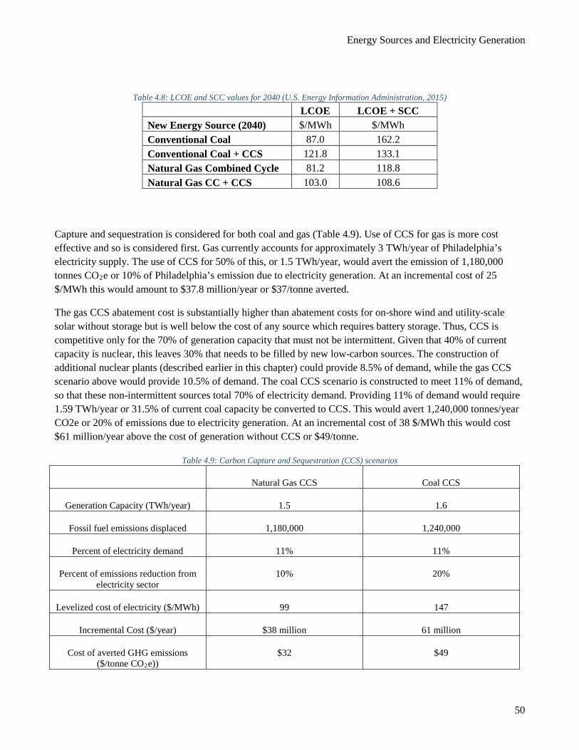
Energy Sources and Electricity Generation

50

Table 4.8: LCOE and SCC values for 2040 (U.S. Energy Information Administration, 2015) LCOE LCOE + SCC

New Energy Source (2040) $/MWh $/MWh Conventional Coal 87.0 162.2 Conventional Coal + CCS 121.8 133.1 Natural Gas Combined Cycle 81.2 118.8 Natural Gas CC + CCS 103.0 108.6

Capture and sequestration is considered for both coal and gas (Table 4.9). Use of CCS for gas is more cost effective and so is considered first. Gas currently accounts for approximately 3 TWh/year of Philadelphia’s electricity supply. The use of CCS for 50% of this, or 1.5 TWh/year, would avert the emission of 1,180,000 tonnes CO2e or 10% of Philadelphia’s emission due to electricity generation. At an incremental cost of 25 $/MWh this would amount to $37.8 million/year or $37/tonne averted.

The gas CCS abatement cost is substantially higher than abatement costs for on-shore wind and utility-scale solar without storage but is well below the cost of any source which requires battery storage. Thus, CCS is competitive only for the 70% of generation capacity that must not be intermittent. Given that 40% of current capacity is nuclear, this leaves 30% that needs to be filled by new low-carbon sources. The construction of additional nuclear plants (described earlier in this chapter) could provide 8.5% of demand, while the gas CCS scenario above would provide 10.5% of demand. The coal CCS scenario is constructed to meet 11% of demand, so that these non-intermittent sources total 70% of electricity demand. Providing 11% of demand would require 1.59 TWh/year or 31.5% of current coal capacity be converted to CCS. This would avert 1,240,000 tonnes/year CO2e or 20% of emissions due to electricity generation. At an incremental cost of 38 $/MWh this would cost $61 million/year above the cost of generation without CCS or $49/tonne.

Table 4.9: Carbon Capture and Sequestration (CCS) scenarios

Natural Gas CCS Coal CCS

Generation Capacity (TWh/year) 1.5 1.6

Fossil fuel emissions displaced 1,180,000 1,240,000

Percent of electricity demand 11% 11%

Percent of emissions reduction from electricity sector

10% 20%

Levelized cost of electricity ($/MWh) 99 147

Incremental Cost ($/year) $38 million 61 million

Cost of averted GHG emissions ($/tonne CO2e))

$32 $49

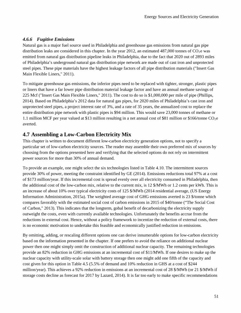
Energy Sources and Electricity Generation

51

4.6.6 Fugitive Emissions Natural gas is a major fuel source used in Philadelphia and greenhouse gas emissions from natural gas pipe distribution leaks are considered in this chapter. In the year 2012, an estimated 487,000 tonnes of CO2e was emitted from natural gas distribution pipeline leaks in Philadelphia, due to the fact that 2020 out of 2893 miles of Philadelphia’s underground natural gas distribution pipe network are made out of cast iron and unprotected steel pipes. These pipe materials have the highest leakage factors of all pipe distribution materials ("Insert Gas Main Flexible Liners," 2011).

To mitigate greenhouse gas emissions, the inferior pipes need to be replaced with tighter, stronger, plastic pipes or liners that have a far lower pipe distribution material leakage factor and have an annual methane savings of 225 Mcf ("Insert Gas Main Flexible Liners," 2011). The cost to do so is $1,000,000 per mile of pipe (Phillips, 2014). Based on Philadelphia’s 2012 data for natural gas pipes, for 2020 miles of Philadelphia’s cast iron and unprotected steel pipes, a project interest rate of 3%, and a rate of 35 years, the annualized cost to replace the entire distribution pipe network with plastic pipes is $94 million. This would save 23,000 tonnes of methane or 1.1 million MCF per year valued at $13 million resulting in a net annual cost of $81 million or $166/tonne CO2e averted.

4.7 Assembling a Low-Carbon Electricity Mix This chapter is written to document different low-carbon electricity generation options, not to specify a particular set of low-carbon electricity sources. The reader may assemble their own preferred mix of sources by choosing from the options presented here and verifying that the selected options do not rely on intermittent power sources for more than 30% of annual demand.

To provide an example, one might select the six technologies listed in Table 4.10. The intermittent sources provide 30% of power, meeting the constraint identified by GE (2014). Emissions reductions total 97% at a cost of $173 million/year. If this incremental cost is spread evenly over all electricity consumed in Philadelphia, then the additional cost of the low-carbon mix, relative to the current mix, is 12 $/MWh or 1.2 cents per kWh. This is an increase of about 10% over typical electricity costs of 125 $/MWh (2014 residential average, (US Energy Information Administration, 2015a). The weighted average cost of GHG emissions averted is 23 $/tonne which compares favorably with the estimated social cost of carbon emissions in 2015 of $40/tonne (“The Social Cost of Carbon," 2013). This indicates that the longterm, gobal benefit of decarbonizing the electricity supply outweight the costs, even with currently available technologies. Unfortunately the benefits accrue from the reductions in external cost. Hence, without a policy framework to incentize the reduction of external costs, there is no economic motivation to undertake this feasible and economically justified reduction in emissions.

By omitting, adding, or rescaling different options one can derive innumerable options for low-carbon electricity based on the information presented in the chapter. If one prefers to avoid the reliance on additional nuclear power then one might simply omit the construction of additional nuclear capacity. The remaining technologies provide an 82% reduction in GHG emissions at an incremental cost of $11/MWh. If one desires to make up the nuclear capacity with utility-scale solar with battery storage then one might add one fifth of the capacity and cost given for this option in Table 4.5 (5.5% of demand and 10% reduction in GHS at a cost of $244 million/year). This achieves a 92% reduction in emissions at an incremental cost of 28 $/MWh (or 21 $/MWh if storage costs decline as forecast for 2017 by Lazard, 2014). It is far too early to make specific recommendations

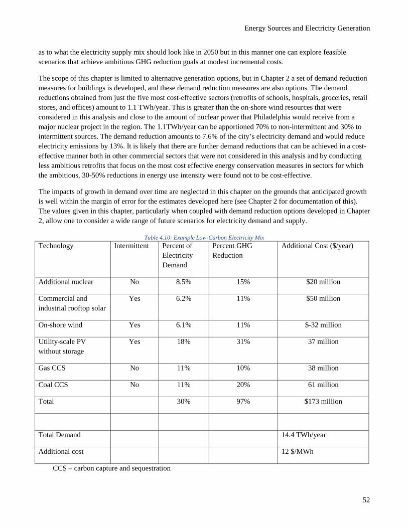
Energy Sources and Electricity Generation

52

as to what the electricity supply mix should look like in 2050 but in this manner one can explore feasible scenarios that achieve ambitious GHG reduction goals at modest incremental costs.

The scope of this chapter is limited to alternative generation options, but in Chapter 2 a set of demand reduction measures for buildings is developed, and these demand reduction measures are also options. The demand reductions obtained from just the five most cost-effective sectors (retrofits of schools, hospitals, groceries, retail stores, and offices) amount to 1.1 TWh/year. This is greater than the on-shore wind resources that were considered in this analysis and close to the amount of nuclear power that Philadelphia would receive from a major nuclear project in the region. The 1.1TWh/year can be apportioned 70% to non-intermittent and 30% to intermittent sources. The demand reduction amounts to 7.6% of the city’s electricity demand and would reduce electricity emissions by 13%. It is likely that there are further demand reductions that can be achieved in a cost-effective manner both in other commercial sectors that were not considered in this analysis and by conducting less ambitious retrofits that focus on the most cost effective energy conservation measures in sectors for which the ambitious, 30-50% reductions in energy use intensity were found not to be cost-effective.

The impacts of growth in demand over time are neglected in this chapter on the grounds that anticipated growth is well within the margin of error for the estimates developed here (see Chapter 2 for documentation of this). The values given in this chapter, particularly when coupled with demand reduction options developed in Chapter 2, allow one to consider a wide range of future scenarios for electricity demand and supply.

Table 4.10: Example Low-Carbon Electricity Mix Technology Intermittent Percent of

Electricity Demand

Percent GHG Reduction

Additional Cost ($/year)

Additional nuclear No 8.5% 15% $20 million

Commercial and industrial rooftop solar

Yes 6.2% 11% $50 million

On-shore wind Yes 6.1% 11% $-32 million

Utility-scale PV without storage

Yes 18% 31% 37 million

Gas CCS No 11% 10% 38 million

Coal CCS No 11% 20% 61 million

Total 30% 97% $173 million

Total Demand 14.4 TWh/year

Additional cost 12 $/MWh

CCS – carbon capture and sequestration

Policy

53

5 COMPARISON OF OPTIONS 5.1 Abstract Emissions reductions options in different sectors are reviewed to identify the least costly set of steps that can achieve targeted reductions. The retrofit of hospitals, schools, grocery stores, and retail establishment, increased use of walking, bicycling, and public transport, and use of on-shore wind power are estimated to have negative abatement costs. Additional commercial building retrofits and the decarbonization of the electricity supply are estimated to be achievable at modest costs that are substantially below the social cost of carbon. While 80% emissions reductions from the building energy and transportation sector are technically feasible, it is more cost effective to achieve 80% reductions by fully decarbonizing the electricity supply. If an 80% reduction is targeted, then fully decarbonizing the electricity supply allows one to avoid some of the most expensive building retrofits (including retrofits in the residential sector and some commercial sectors) but the full 80% reduction in transportation emissions would be required. A target of 66% reduction in emissions would substantially reduce the required adoption of plug-in hybrid electric vehicles in the transportation sector. Current cost estimates for plug-in hybrids exceed estimates of the current social cost of carbon, but subsequent technology development is expected to reduce costs.

A set of priorities for research and policy discussions are identified, including studies of sectors not considered in this report, such as waste disposal, fugitive emissions from landfills, industrial processes and many other areas. More detailed follow up studies are also needed in many areas considered by this report, such as whether nuclear power and carbon capture and sequestration should be part of greenhouse gas emissions reduction efforts. Discussion of emissions reduction plans may emphasize that options for achieving greenhouse gas emissions reductions are currently feasible and do not involve foregoing the benefits of modern technology. Further development of technology over time may provide new and less expensive means of achieving these emissions reduction goals.

5.2 Comparing Sectors In this chapter the abatement costs of the different option are compared across sectors to identify where reduction may be made in a cost-effective manner. While this analysis cannot identify the set of technologies that should be adopted in 2050 with certainty, it is intended to identify priorities for consideration and study.

The first step in seeking to cut emissions is to identify any areas where emissions abatement costs are negative, as such emissions reductions should yield cost savings. In this analysis three areas with negative abatement costs were identified.

1) Four of the seven commercial building types considered had negative emissions abatement costs (Hospitals, schools, grocery stores, and retail establishments). Reduction in these sectors alone would save 4.6% of all energy used in the building sector and reduce GHG emissions by 6.7%. If similar opportunities could be found in the sectors not considered in detail in this report, then demand reductions of 22% and emissions reductions of 32% would be achieved.

2) On-shore wind power is a second area where emissions abatements may be negative, as long as the percentage of total intermittent sources is small enough that storage is not required. This study suggested that meeting 6.1% of demand might be feasible, which would reduce emissions from the electricity sector by 11%.

Policy

54

3) Transportation mode shifts away from automobiles and toward walking, bicycling, and greater use of public transit likely have negative abatement costs in many cases, but an economic analysis of these options would be complicated by the intangibles involved and variability in individual circumstances. Very ambitious assumptions of greater use of these modes yield roughly a 10% drop in emissions from the transport sector. Realistically, these options are probably limited to obtaining a reduction of a few percent in transportation emissions, unless significant changes are made that encourage those mode choices, such as denser use of land, provision of additional public transit options, dedicated bicycle paths, policy measures that constrain the use of automobiles, etc.

Once areas of negative abatement costs are identified, one looks for the set of least expensive options that will achieve the desired reductions. In order these appear to be:

1. Energy efficiency upgrades for commercial offices appear favorable at $6/tonne averted. If these retrofits in the office sector are made in addition to the retrofits in the four sectors with negative abatement costs, then the total reduction in demand would amount to 7.6%. If similar opportunities could be found in sectors not studied in this report, then this would reduce demand by 36% and emissions by 53%.

2. De-carbonization of the electricity supply appears to be very attractive with an estimated abatement cost of $23/tonne for 97% reductions in this sector.

3. Transportation emissions beyond the few percentage reductions available through mode shifts rely greatly on the use of plug-in electric hybrid vehicles which have an estimated abatement cost of $90/tonne.

4. The extensive retrofits of the kind evaluated here have costs of >$100/tonne avoided for many residential and commercial sectors.

It is of interest that energy efficiency opportunities in buildings constitute among the most attractive and least attractive of the abatement strategies considered here. De-carbonization of the electricity supply is more cost-effective than a portion of the building energy demand reductions. Thus, an 80% reduction in GHG emissions can be achieved without the full 80% building energy demand reduction that is technically feasible, and in fact it would be most economically efficient to maximize the decarbonization of the electricity supply in place of conducting the least cost-effective building retrofits. If the electricity supply is fully decarbonized, then a reduction in gas use of 41% would enable the overall building sector emissions to be reduced by 80%. This study cannot provide assurances that such a substantial reduction in gas use is possible in a cost-effective manner as not all sectors were studied. However, if the same amount of demand reduction opportunities are found in the sectors not yet studied, then (as noted above) a 22% reduction in building energy demand can be justified without any consideration of GHG emissions benefits. If only gas GHG emissions reductions are counted, then the office sector has an abatement cost of $46/tonne. The remaining emissions reductions would then need to be obtained in the transportation sector with many of these abatements due to PHEV adoption which has an estimated cost of $90/tonne.

If the target reduction in GHG emissions for transportation and buildings is relaxed from 80% to 66% reduction (that is, the reduction corresponding to reducing emissions to 80% of the national per capita average), then this can almost be achieved through decarbonization of the electricity supply and a 41% reduction in gas use. The 80% reduction in the 60% of emissions associated with the buildings sector amounts to a reduction of only 61%

Policy

55

in combined emissions from both sectors (assuming transport is 19% of current emissions). A 22% reduction in transportation emissions would be necessary to provide for a combined reduction of 66%.

To summarize, based on the costs and extent of abatement opportunities found in this study, efforts to reduce GHG emissions should begin with energy efficiency retrofits in the commercial buildings sector, proceed to decarbonization of the electricity supply, then to additional building energy demand reduction efforts, and finally to the adoption of PHEVs in the transportation sector. If an 80% overall reduction is desired, then roughly 80% reductions will need to be made in transportation through widespread adoption of PHEVs; while if a 66% reduction is targeted, then more limited adoption of PHEVs would be required. Initial abatement opportunities have negative abatement costs, very substantial reductions are available in the electricity sector for well below the current social cost of carbon (average abatement cost of $23/tonne vs. current estimate of the social cost of carbon as roughly $40/tonne), and the final abatements obtained through the use of PHEVs may exceed current estimates of the social cost of carbon given currently available PHEV technology. Future innovation may reduce PHEV costs to the point where abatement costs become negative (NYC 2013). This provides a basis for delaying widespread adoption of current PHEV technologies. In contrast, decarbonization of the electricity supply appears feasible and cost-effective with current technology.

In reviewing these options it is important to be mindful of the many limitations of this analysis. While this analysis suggests that residential energy efficiency retrofits are not cost-effective, the report considered only very ambitious and expensive retrofits. Less ambitious retrofits may well be justified in the residential sector. Thus further study might be devoted to examining particular energy conservation measures that may be adopted without extensive retrofits and may be cost-effective for the residential sector. The analysis also did not consider densification of population, provision of additional public transportation infrastructure, and other large-scale changes to infrastructure. While these options are difficult to evaluate, they may offer substantial benefits.

In addition, this study did not consider all sources of emissions but rather focused on three important sectors. Achieving overall emissions reductions requires that savings from other sectors, including waste disposal, industry, etc. are able to match the emissions reductions found in the sectors considered here.

5.3 Next Steps The goal of this analysis is not to specify the technologies to be used in 2050, much less to specify a time table for the adoption of specific measures. By identifying some steps that are immediately cost-effective, the analysis may guide initial steps along the pathway to deep reductions in GHG emissions. In addition, by identifying some challenges it may point to where further study, technological development efforts, and negotiations among stakeholders are called for. Several areas where this report may inform future research, stakeholder discourse, and policy formulation are as follows:

• The report clearly identifies options for achieving 80% reductions in GHG emissions that are technologically feasible with existing technology. This conclusion may be used to counter ideas that reductions in GHG emissions involve foregoing the benefits of modern technology through reversion to a pre-industrial society.

• The incremental costs of the deepest reductions appear to exceed the social cost of carbon emissions. This is expected to no longer be the case by 2050 but may be a valid argument for

Policy

56

delaying the implementation of these measures pending both further study of technological options and the development of new technological options through research and development.

• Initial efforts at GHG reduction may focus on energy efficiency in buildings. The potential of energy efficiency varies widely. Many but not all of these measures are cost-effective based on utility bills savings alone. In contrast, some deep retrofits in the residential sector and in select commercial building types are not a cost-effective means of achieving 80% emissions reductions compared to de-carbonization of the electricity supply. The City’s building energy benchmarking program is an example of an effort to better identify where these emissions reduction opportunities exist. The information in this report may help target some sectors for further programmatic efforts, including provision of information, development of data and estimation tools to support decision making by owners, and access to capital.

• The results of this report also suggest that more detailed study is needed of other commercial sectors to assess if the energy savings found in the 7 commercial sectors studied here can also be found in other sectors not yet studied.

• Further study is also needed of the residential sector. While ambitious retrofits aimed at 30-50% reduction did not appear cost-effective, it is likely that a number of energy conservation measures are cost-effective and these less comprehensive measures may nevertheless have considerable potential when applied to the large residential housing sector.

• The report suggests that de-carbonization of the electricity supply is feasible at moderate cost with present technology. However the precise manner in which this should be accomplished has not been specified and would require considerable study and public debate. Businesses and private individuals might need to be more involved in accommodating load shedding during times of peak demand to accommodate intermittent electricity sources. A decision as to the renewal of licenses of existing nuclear plants and potentially even expansion of the nuclear portion of the electricity supply raises many technical questions and policy issues that would need to be evaluated including the location of the facilities and whether concerns over waste transport, storage, and long term disposal can be addressed satisfactorily. Similar questions arise with the use of carbon capture and sequestration which would require a large and expensive infrastructure and has its own safety concerns. Even the use of solar generation raises questions that require further technical analysis and public discussion such as the location of the facilities, the expected financial returns in an area with moderate insolation and high land costs, whether additional rights of way for transmission lines would be required, and so forth.

• Both electricity demand reductions from building energy efficiency and demand increases due to widespread adoption of PHEVs are substantial and may need to be accounted for in future planning.

• This report did not consider how additional public transportation infrastructure might affect emissions. The development of a more detailed transportation simulation model would be an important tool for analyzing such alternatives.

• This report was limited in terms of the sectors that were addressed. The additional Scope 1 emissions from sources such as the airport, port, and water/wastewater treatment were not explicitly analyzed, and options have not been developed as to how to achieve reductions in those areas. The study of these sectors is a priority for future work.

Given that this report does not provide a roadmap to achieving 80% reductions by 2050, but rather a set of priorities for study and discussion, the question becomes how such study and discussion should be carried out.

Policy

57

Climate change policy formulation is a relatively new responsibility of cities, and best practices and performance benchmarks are not yet available. However, a number of cities have undertaken climate policy formulation and the processes used in different cities may be compared to identify alternative strategies for consideration. Such a review and comparison is conducted in Chapter 6 of this report.

Policy

58

6 POLICY

6.1 Abstract While the precise set of technologies and policies needed to achieve deep cuts in greenhouse gas emissions cannot be specified at this time, what is needed now is a climate change policy process capable of identifying and implementing the most effective technologies and initiatives. Cities are becoming recognized as a vital level of climate change policy making, and many cities have already developed institutional approaches toward these efforts. This chapter reviews the approaches taken by ten large U.S. cities, including Philadelphia. Policy process structures in each city are characterized as either dedicated, in which a single entity in the city government implements climate change policy, or as mainstreaming, in which entities throughout city government implement climate change policies within their own domains. Policy implementation approaches are characterized as either governmental action, in which the city government directly takes the action, or as public-private partnership action, in which the city acts in concert with other stakeholders in the region. Five of the ten cities studied, including Philadelphia, employ a mainstreaming structure with a public-private partnership action approach to implementation. This approach appears well suited to achieving broad impacts that are required to substantially reduce carbon emissions. However, dedicated efforts may still be appropriate in certain circumstances and governmental action opportunities should not be ignored should they be available. Future efforts should include a careful observation of the policy processes undertaken by peer cities and an evaluation of the effectiveness of these different policy development approaches.

6.2 Introduction The preceding chapters develop specific scenarios for how deep emissions in carbon dioxide can be achieved in the transportation, building, and electrical generation sectors. The adoption of these measures will require far-reaching transformations of large technical systems and their attendant socio-technical relations of production and consumption. In some views these scenarios would be realized through a focused and purposeful transition, with government orchestrating society’s more or less orderly march toward a more sustainable future (Bulkeley, Catán Broto, & Edwards, 2015, p. 237). The last quarter century of climate change policy, in the United States and elsewhere, inspires little confidence in this view of innovation and change. Large technical systems and the socio-technical networks in which they are embedded have shown remarkable obduracy in the face of anthropogenic climate change. Meeting the challenge to transform these systems may require coordination and forethought beyond what the human race has manifested in the past (Dryzek, Norgaard, & Schlosberg, 2013, p. 15).

Given the global scale of the issue, international agreements, such as the Kyoto protocol, have often been seen as the mechanism for meeting this challenge. However, recent studies (Bulkeley, 2010; Bulkeley et al., 2014; Carter et al., 2015; Castán Broto & Bulkeley, 2013; Sharp et al., 2011; Uittenbroek et al., 2014) have begun to focus on the city as a main driver of climate change policy. While the uniform requirements needed to address a global issue through regulatory action would need to be negotiated among national governments, cities have a role to play as test beds of potential strategies and as information providers that may influence national governmental policy. In addition, cities must seek to prepare for a carbon constrained world by identifying pathways for emissions mitigation that will allow them to remain economically competitive and continue to provide the amenities desired by their citizens.

Policy

59

Due to all these factors, the city is now a major relevant site for creating and implementing strategies to combat climate change (Bulkeley, Edwards, & Fuller, 2014; Sharp, Daley, & Lynch, 2011). Indeed, the existence of policy networks such as the International Council for Local Environmental Initiatives (ICLEI) and the Urban Sustainability Directors Network (USDN) enable urban climate change professionals from all over the world to share data and information from their efforts. These efforts foster successful new climate mitigation and adaptation strategies, indicating that it is increasingly at the city level where innovative climate change policy decisions are being made.

To develop and implement climate change policies, cities need a deliberative process that identifies and addresses local aspects of how such policies should be implemented. The success of emissions reductions may depend greatly on the goals of the stakeholders, the governmental structure, and the process by which these policy choices are made (Uittenbroek, Janssen-Jansen, Spit, Salet, & Runhaar, 2014; Bulkeley & Betsill, 2013). This policy process may involve contestation and cooperation with and across Philadelphia’s socio-technical networks. The need for cooperation is self-evident, given the multitude of actors and institutions at various scales - public, private, local, state, and federal - that are implicated in large technical systems and that must work together in order to move forward. Contestation, however, could help turn governance networks into more productive deliberative systems by bringing to the fore explicitly normative questions about sustainable urban infrastructure: What do we want it to be? Who is it for? Is it effective, but also just? (Dryzek, Norgaard, and Schlosberg, 2013, p. 145). Barring massive external shocks and concerted international action, it is unlikely that large technical systems, urban or otherwise, will somehow decarbonize themselves, and so part of the challenge for an effective urban politics of climate change is to open up expert-dominated infrastructure networks to a wider spectrum of stakeholders and to public contestation.

Many cities are currently engaged in a variety of efforts to tackle the challenges of climate change (Castán Broto & Bulkeley, 2013). Efforts are also underway to benchmark the progress of cities toward achieving emissions reductions (GGP, 2015). However, data on the actual performance of different cities on achieving climate change mitigation goals is not generally available. In the absence of systematic performance data, a review of institutions may provide some insight into what cities are establishing the capability to formulate policy processes that will lead to emissions reductions. With this goal in mind, this chapter compares the climate change policy formulation processes used in ten major U.S. cities. The chapter first describes different categories of climate change policy processes and then applies this classification system to the climate change policy processes of ten U.S. cities, including Philadelphia. Finally, Philadelphia’s policy processes are compared with those of the other cities and potentially beneficial approaches, as well as remaining challenges, are identified.

6.3 Climate Policy Process Categories Uittenbroek et al. have identified two main organizational structures that municipal governments use to respond to climate change: the dedicated organizational structure and the mainstreaming organizational structure (2014). In the dedicated approach, “climate adaptation is presented as a new policy domain,” (Uittenbroek et al., 2014) apart from other policy domains such as housing, transportation, employment. The mainstreaming approach, on the other hand, “aims to integrate climate adaptation into existing policy domains such as spatial planning, water management, and public health” (Uittenbroek et al., 2014). Essentially, if a city’s Office of Planning were to include energy efficiency and GHG emissions considerations as part of its standard decision-making process—if a given city department or agency is able to act on climate change in the course of its standard operations, to integrate climate change considerations with those operations—then that is an example of the mainstreaming

Policy

60

approach. Here, policy entrepreneurs find ways to synergize climate change policy with these preexisting city commitments.

Both the dedicated and the mainstreaming governmental structures have advantages and disadvantages. For example, the dedicated approach can serve as a boon for climate change planning in that, should a political leader champion the importance of this policy arena, there will be a visible organizational structure for action, and the politicians involved can be held accountable for the results. The dedicated approach, if utilized well, could also result in swift and direct action on climate change. The downside to this approach, however, is that given “the uncertainty and long-term character of climate change, the limited carrying capacity of an agenda, and limited resources” (Uittenbroek et al., 2014), the climate change policies enacted can vary widely or even be neglected completely depending on what person occupies the relevant political leadership position at a given point in time. In other words, there is little institutional assurance that one mayor, for example, will continue to act on climate change as vigorously as his or her predecessor did. A major advantage of the mainstreaming approach, by contrast, is that indirect political commitment to climate change action, dispersed throughout city government and beyond, can be more sustainable over time because it is somewhat less dependent on high-level political leadership. Because municipal climate change action in the mainstreaming approach is somewhat insulated from the whims of elected leaders, there is a greater ability to establish continuity and implement longer-term actions. The downside is that, in the absence of political pressure and sustainable structures, even the most innovative policy entrepreneurs and agency staff may be unable on their own to reallocate resources to meet climate change goals, particularly the ambitious actions needed to substantially reduce emissions. While the mainstreaming approach may lead to a more integrated and sustainable climate change response, its capacity to enact bold new policies may be limited.

Too close a focus only on a city government’s capacity to act on climate change neglects the many ways that individuals and organizations outside city government can also do so. If action on climate change is understood as the implementation of climate change policy by the relevant, affected entities, then the contemporary American city has at its disposal a host of action capabilities within and outside formal governmental structure. In their assessment of urban climate change policy implementation Bulkeley and Betsill (2013) have identified two methods of action: “municipal voluntarism” which we will refer to as “governmental action” in this document and “strategic urbanism” which we will refer to as “public-private partnership action.”

Governmental action is a policy implementation process characterized by individuals within a municipal government recognizing the potential and need to act on climate change and offering responses from within that government structure (Bulkeley & Betsill, 2013). This is a relatively straightforward process, where actors within a city undertake responses to climate change based on either individual or institutional determinations of necessity. This was the standard for urban climate change policy implementation until the early 2000s (Bulkeley & Betsill, 2013). But where the municipal government alone may have been “lacking the political will…to introduce new forms of regulation and [has had] a minimal role in how critical infrastructure systems and utility services were provided,” cities developed “an enabling mode of governing through which business and communities were encouraged to act in, and on behalf of, the city” (Bulkeley & Betsill, 2013). Municipal governments distributed “resources, competencies, and power… horizontally through other spheres of authority and the consequent effects on urban climate governance” (Bulkeley & Betsill, 2013). This sharing of the authority to act on climate change by city governments with “a range of actors, sites and processes through which climate change is being addressed” (Bulkeley & Betsill, 2013) is the basic idea behind the concept of public-private partnership action. With the emergence of this form of policy implementation in American cities,

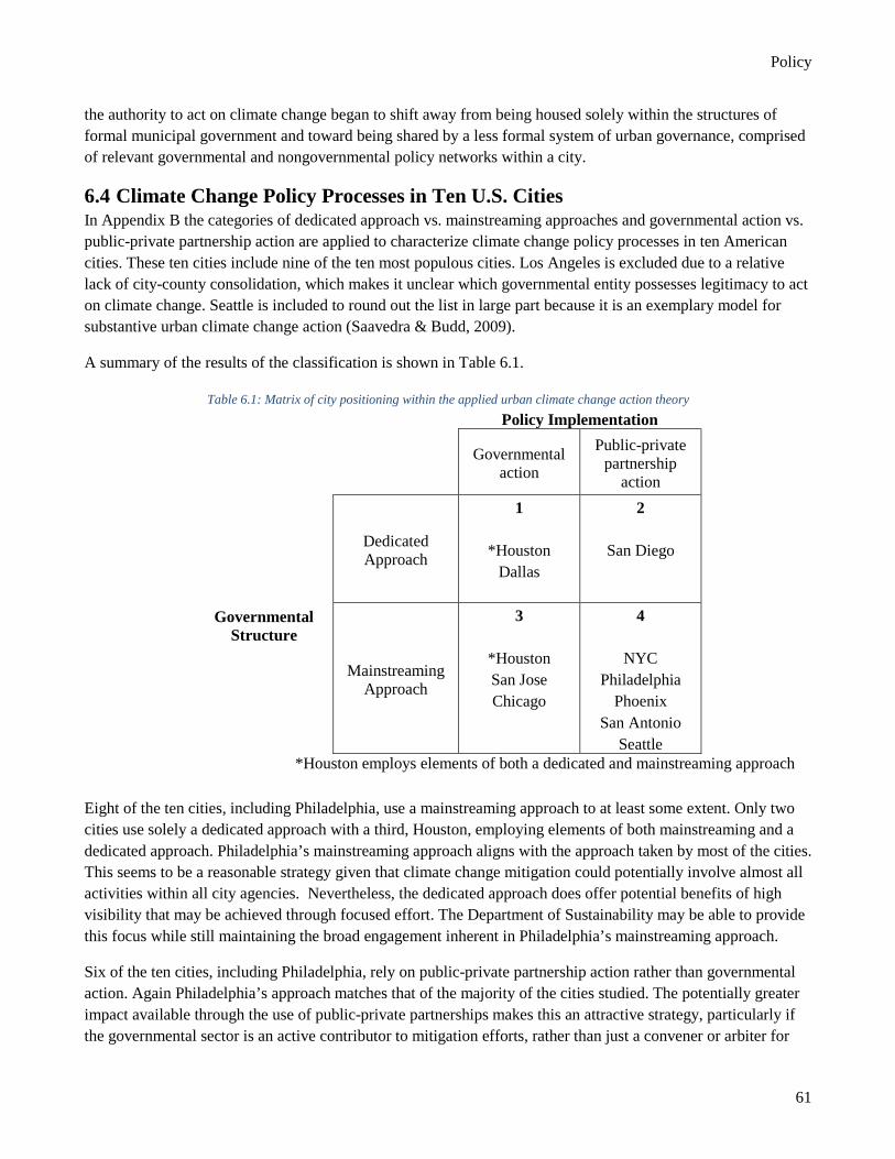
Policy

61

the authority to act on climate change began to shift away from being housed solely within the structures of formal municipal government and toward being shared by a less formal system of urban governance, comprised of relevant governmental and nongovernmental policy networks within a city.

6.4 Climate Change Policy Processes in Ten U.S. Cities In Appendix B the categories of dedicated approach vs. mainstreaming approaches and governmental action vs. public-private partnership action are applied to characterize climate change policy processes in ten American cities. These ten cities include nine of the ten most populous cities. Los Angeles is excluded due to a relative lack of city-county consolidation, which makes it unclear which governmental entity possesses legitimacy to act on climate change. Seattle is included to round out the list in large part because it is an exemplary model for substantive urban climate change action (Saavedra & Budd, 2009).

A summary of the results of the classification is shown in Table 6.1.

Table 6.1: Matrix of city positioning within the applied urban climate change action theory

Policy Implementation

Governmental action

Public-private partnership

action

Governmental Structure

Dedicated Approach

1

*Houston Dallas

2

San Diego

Mainstreaming Approach

3

*Houston San Jose Chicago

4

NYC Philadelphia

Phoenix San Antonio

Seattle *Houston employs elements of both a dedicated and mainstreaming approach

Eight of the ten cities, including Philadelphia, use a mainstreaming approach to at least some extent. Only two cities use solely a dedicated approach with a third, Houston, employing elements of both mainstreaming and a dedicated approach. Philadelphia’s mainstreaming approach aligns with the approach taken by most of the cities. This seems to be a reasonable strategy given that climate change mitigation could potentially involve almost all activities within all city agencies. Nevertheless, the dedicated approach does offer potential benefits of high visibility that may be achieved through focused effort. The Department of Sustainability may be able to provide this focus while still maintaining the broad engagement inherent in Philadelphia’s mainstreaming approach.

Six of the ten cities, including Philadelphia, rely on public-private partnership action rather than governmental action. Again Philadelphia’s approach matches that of the majority of the cities studied. The potentially greater impact available through the use of public-private partnerships makes this an attractive strategy, particularly if the governmental sector is an active contributor to mitigation efforts, rather than just a convener or arbiter for

Policy

62

such efforts. Again the Department of Sustainability may be able to play a key role as facilitator of the public private partnership negotiations, while at the same time ensuring that governmental action is not neglected.

Five of the ten cities, including Philadelphia employ both a mainstreaming and public-private partnership action approach. These two approaches, which maximize the involvement of both city agencies (through mainstreaming) and non-governmental stakeholders (through public-private partnerships), appear to have the greatest potential to produce the broad changes necessary to achieve dramatic reductions in greenhouse gas emissions. However, follow-up is needed to observe if these approaches perform better than other approaches and if any of these approaches are able to facilitate the required transformation to urban energy use.

6.5 Electricity, Building Energy, and Transportation: Policy Challenges for Getting to 80x50

The deep GHG emission reductions proposed here have to contend not only with the obduracy of large technical systems but also with the persistence of the postindustrial urban economic condition. Reducing building energy, for example, will require massive capital investment in what is in many cases a deteriorated housing infrastructure. A poverty rate of around 25% makes Philadelphia the poorest of America’s ten largest cities, and rates of home ownership declined fairly steeply in the wake of the Great Recession. Both of these factors are substantial barriers to investing in a dramatic upgrade of housing stock, particularly in the city’s persistently poor neighborhoods, where real estate development remains an unlikely prospect. It is difficult to see how technological innovation alone could fundamentally alter this stark economic reality—even if some retrofitting technologies likely will become marginally more cost effective due to technological progress.

On the electricity side, one major challenge is that in the absence of concerted national and international action, there are few incentives to embrace a dramatic, though likely feasible transformation in the energy supply mix. Continued switching to natural gas could show some further modest benefits for carbon emissions and might satisfy the EPA’s existing standards for carbon pollution from new and existing power plants, but will not achieve 80% reduction. Extending the operating licenses of the region’s nuclear plants appears to be feasible, but without retrofits and new plant construction there is considerable uncertainty in the ability to maintain nuclear capacity beyond 2050. Whether nuclear energy’s 80x50-relevant advantages (low-carbon, base-load power reliability) can overcome its liabilities (facility siting, waste disposal, weakening long-term demand) is very much an open question. If the share of nuclear power were to decline following plant decommissioning, electricity generation might—absent other developments—become more carbon intensive rather than less carbon intensive. Fortunately, technological innovation is likely to make electricity generation from renewable sources—wind, solar—preferable to fossil fuels on economic grounds, but for renewables to exceed 30% of the energy supply mix may require a significant breakthrough on storage costs. Integrating wind and solar into the energy supply mix is also hampered by current utility business models. Current renewable technology and falling prices are already making distributed resources extremely competitive, and as storage prices fall they will become even more so. However, utilities need to be supported by state and federal regulation to allow them to be “paid” for grid services, unbundled from the volume of electrons they sell. Put simply, they will need to be compensated for maintaining the grid and for balancing supply and demand as they integrate distributed resources.

Transportation and transportation planning are rife with examples of the stubborn persistence of large technical systems and the momentum of the status quo. Rolling out alternative fuel vehicles promises significant reductions in GHG emissions, but such vehicles fail to address some of the key challenges associated with

Policy

63

private vehicle mobility. For example, even after addressing issues such as electricity generation and infrastructure to support the widespread adoption of electric vehicles, the latter will not solve congestion problems and might even encourage further expansions of urban areas. In this way, reducing the carbon footprint of privately owned vehicles may actually impede rather than advance the achievement of sustainable mobility. Urban planning is key to the achievement of sustainable transportation. Policies encouraging the densification of urban areas, limiting sprawl, and encouraging infill development will affect travel decisions at the individual and household level. Transit investments, the densification of urban development around transit corridors, and investments in infrastructure supporting active mobility, are examples of policies that are often associated with small GHG reductions when evaluated in exercises like this one. This is because we tend to be conservative in our projections of future investments in transit (or other) infrastructure considering its high capital costs borne by governments. Future transit expansion scenarios are limited by “what is already on the table” in terms of planned transit projects. It is difficult to identify and evaluation feasible alternative futures with drastically different urban transportation and transit structures.

This report does not offer specifics for addressing these barriers, nor could a single report surmount all of them. Instead it seeks to affirm that alternative technologies do exist that could effectively provide energy while dramatically reducing carbon emissions. Selecting from these infrastructures and policies is not the work of a single report written in 2015 but of an ongoing process. This chapter is intended to inform the continuation and strengthening of this process by reviewing how Philadelphia’s efforts align with those of other cities. Ongoing comparisons and exchanges with other cities can further inform Philadelphia’s efforts in the future.

References

64

7 REFERENCES Argonne National Labrotary. (2014). GREET model: Transportation Technology R & D Center, US Department

of Energy. ASHRAE. (August, 2008). "Advanced Energy Design Guide for Small Warehouses and Self Storage Buildings: Achieving 50% Energy Savings Toward a Net Zero Energy Building". American Society of Heating, Refrigeration, and Air-Conditioning Engineers. ASHRAE. (April, 2011). "Advanced Energy Design Guide for Small to Medium Office Buildings: Achieving 50% Energy Savings Toward a Net Zero Energy Building". American Society of Heating, Refrigeration, and Air-Conditioning Engineers. ASHRAE. (September, 2011). "Advanced Energy Design Guide for K-12 School Building: Achieving 50% Energy Savings Toward a Net Zero Energy Building". American Society of Heating, Refrigeration, and Air-Conditioning Engineers. ASHRAE. (May, 2012). "Advanced Energy Design Guide for Large Hospitals: Achieving 50% Energy Savings Toward a Net Zero Energy Building." American Society of Heating, Refrigeration, and Air-Conditioning Engineers. ASHRAE. (April, 2014). "Advanced Energy Design Guide for Medium to Big Box Retail Buildings: Achieving 50% Energy Savings Toward a Net Zero Energy Building." American Society of Heating, Refrigeration, and Air-Conditioning Engineers. ASHRAE. (March, 2015). "Advanced Energy Design Guide for Grocery Stores: Achieving 50% Energy Savings Toward a Net Zero Energy Building". American Society of Heating, Refrigeration, and Air-Conditioning Engineers. Bhatia, A., B.E. “HVAC Made Easy: A Guide to Heating & Cooling Load Estimation.” PDH Online, 2012.

Retrieved August 1, 2015 from http://www.pdhonline.org/courses/m196/m196.htm. Bloomberg, M. (2006). "Long Term Planning in New York City -- Challenges and Goals." Gotham Gazette.

Retrieved 28 Jan., 2015, from http://www.gothamgazette.com/index.php/open-government/3441-long-term-planning-in-new-york-city-challenges-and-goals-#

Bulkeley, H. (2010). Cities and the Governing of Climate Change. Annual Review of Environment and

Resources, 35(1), 229-253. doi: doi:10.1146/annurev-environ-072809-101747 Bulkeley, H., & Betsill, M. M. (2013). Revisiting the urban politics of climate change. Environmental Politics,

22(1), 136-154. doi: http://dx.doi.org/10.1080/09644016.2013.755797 Bulkeley, H., Edwards, G. A. S., & Fuller, S. (2014). Contesting climate justice in the city: Examining politics

and practice in urban climate change experiments. Global Environmental Change, 25(0), 31-40. doi: http://dx.doi.org/10.1016/j.gloenvcha.2014.01.009

Burtraw, D., & Krupnick, A. (2012). The True Cost of Electric Power. Center for Energy Economics and Policy,

Resources for the Future, Retrieved September 6, 2015,

References

65

from: http://www.ren21.net/Portals/0/documents/Resources/RFF-Rpt-BurtrawKrupnick.TrueCosts_Summary_web.pdf

Carter, J. G., Cavan, G., Connelly, A., Guy, S., Handley, J., & Kazmierczak, A. (2015). Climate change and the

city: Building capacity for urban adaptation. Progress in Planning, 95(0), 1-66. doi: http://dx.doi.org/10.1016/j.progress.2013.08.001

Castán Broto, V., & Bulkeley, H. (2013). A survey of urban climate change experiments in 100 cities. Global

Environmental Change, 23(1), 92-102. doi: http://dx.doi.org/10.1016/j.gloenvcha.2012.07.005 Census Bureau. (2015). Philadelphia County QuickFacts. Center for Climate and Energy Solutions. (2015). EPA Regulation of Greenhouse Gas Emissions from New

Power Plants. from http://www.c2es.org/federal/executive/epa/ghg-standards-for-new-power-plants Citizens Environmental Advisory Committee. (2014). sanantonio.gov. Retrieved 28 Jan., 2015,

from http://www.sanantonio.gov/sustainability/OrdinancesAndGovernance/EnvironmentalAdvisoryCommittee.aspx

City of Boston. (2015a). Greenovate Boston. 2014 Climate Action Plan Update Retrieved September 20, 2015, From http://plan.greenovateboston.org/

City of Boston. (2015b). Boston's Greenhouse Gas Emissions. Retrieved May 03, 2015,

from http://www.cityofboston.gov/climate/progress/tracking.asp City of Chicago. (2008). Chicago Climate Action Plan. Chicago, IL: City of Chicago. City of Chicago. (2015) Sustainable Chicago Action Agenda 2015 Chicago Sustainability Council. City of

Chicago, Chicago, IL. City of Houston. (2008). Green Houston: Emissions Reduction Plan, August 2008. Houston, Texas: City of

Houston. Retrieved from: http://www.greenhoustontx.gov/reports/emissionreduction20080909.pdf. City of Houston. (2009). Green Houston: Emissions Reduction Plan Updated, December 2009. Houston, Texas:

City of Houston. Retrieved from: http://www.greenhoustontx.gov/reports/emissionreduction20091217.pdf.

City of Houston. (2015). About the Sustainability Director. greenhoustontx.gov. Retrieved 28 Jan., 2015,

from http://www.greenhoustontx.gov/spanjian.html. City of Philadelphia. (2015). About the Mayor's Office of Sustainability. retrieved from Retrieved 28 Jan., 2015,

from http://www.phila.gov/green/about.html. City of Phoenix Organizational Chart. (2015). phoenix.gov. Retrieved 28 Jan., 2015, from

https://www.phoenix.gov/citymanagersite/Documents/CityofPhoenixOrganizationChart.pdf City of Phoenix. (2015). Climate Change. Retrieved from: https://www.phoenix.gov/oep/environment/climate City of San Diego Departments. (2015). City of San Diego. Retrieved 28 Jan., 2015,

from http://www.sandiego.gov/

References

66

City of San Diego Planning Department. (2005). Climate Protection Adaptation Plan. City of San Diego. City of San Diego Environmental Services Department. Connections. (2015). sandiego.gov. Retrieved 28 Jan.,

2015, from http://www.sandiego.gov/environmental-services/sustainable/connect.shtml City of San Diego Environmental Services Department. Index. (2015). sandiego.gov. Retrieved 28 Jan., 2015,

from http://www.sandiego.gov/environmental-services/sustainable/index.shtml Climate Change. (2015). seattle.gov/environment. Retrieved 28 Jan., 2015,

from http://www.seattle.gov/environment/climate-change Climate Change: Programs & Policies. (2015). seattle.gov/environment. Retrieved 28 Jan., 2015,

from http://www.seattle.gov/environment/climate-change/programs-and-policies CMD. (2015). “Elevators Cost Estimating Tips,” Smart Building Index, Construction Market Data, retrieved on

September 22, 2015 from http://www.cmdgroup.com/smartbuildingindex/elevators/costs/. Connor, A. M., & Francfort, J. E. U.S. Hydropower Resource Assessment for Pennsylvania. Copengagen Economics. (2012). Multiple benefits of investing in energy efficient renovation of buildings.

Copenhagen Economics. Delaware Valley Regional Planning Commission (2013a). Analytic Data Report 19: Regional, County, and

Municipal Employment Forecasts, 2010-204. Retrieved October 1, 2015 from http://www.dvrpc.org/reports/ADR019.pdf.

Delaware Valley Regional Planning Commission (2013b). Analytical Data Report 18-A: Regional, County, and

Municipal Employment Forecasts, 2010-2040. Retrieved October 1, 2015 from http://www.dvrpc.org/reports/ADR018-A.pdf.

Delaware Valley Regional Planning Commission. (2014a). Amended transportation investments: Connections

2040-Plan for greater Philadelphia: Delaware Valley Regional Planning Commission. Delaware Valley Regional Planning Commission. (2014b). Energy use and greenhouse gas emissions in greater

Philadelphia: 2010 summary: Delaware Valley Regional Planning Commission. Delaware Valley Regional Planning Commission. (2015). 2012 Household Travel Survey. Retrieved March

02, 2015, from http://www.dvrpc.org/Transportation/Modeling/Data.htm Deputy City Manager Rick Naimark. (2015). phoenix.gov. Retrieved 28 Jan., 2015, from

https://www.phoenix.gov/citymanager/executive-team/rick-naimark eGRID 9th Edition Version 1.0. (2014). Retrieved March 31, 2015 Energy Alliances. (2015). sandiego.gov. Retrieved 28 Jan., 2015, from http://www.sandiego.gov/environmental-

services/energy/programsprojects/alliances.shtml Energy Star. (2015). "ES Lighting Lifetime Savings." EnergyStar, retrieved August 1, 2015

from http://www.energystar.gov/ia/products/images/ES_Lighting_LifetimeSavings.jpg.

References

67

Energy Star Portfolio Manager (2014). Technical Reference: Greenhouse Gas Emissions. Energy Star 2013. Energy Star Certified Homes, Version 3, Costs & Savings Estimates. U.S. Environmental

Protection Agency, retrieved on September 14, 2015 from: https://www.energystar.gov/ia/partners/bldrs_lenders_raters/downloads/EstimatedCostandSavings.pdf?0544-2a1e

Environmental Coordinating Council. (2015). greenhoustontx.gov. Retrieved 28 Jan., 2015,

from http://www.greenhoustontx.gov/ecc.html Environmental Management System. (2015). dallascityhall.com. Retrieved 28 Jan., 2015,

from http://dallascityhall.com/departments/OEQ/Pages/ems.aspx Environmental Quality Commission Initiatives. (2015). phoenix.gov. Retrieved 28 Jan., 2015, from

https://www.phoenix.gov/oep/eqc/initiatives Environmental Quality Commission Member Profiles. (2015). phoenix.gov. Retrieved 28 Jan., 2015, from

https://www.phoenix.gov/oep/eqc/member-profiles Environmental Protection Agency. (2012). Mercury and Air Toxics Standard. Environmental Protection

Agency, March 27, 2012, from http://www.epa.gov/mats/ Environmental Protection Agency. (2014). Emissions & Generation Resource Integrated Database,

Environmental Protection Agency Environmental Protection Agency. (2014). What EPA is Doing. Environmental Protection Agency, Retrieved

June 4, 2015, from http://www2.epa.gov/carbon-pollution-standards/what-epa-doing Environmental Protection Agency. (2015). Greenhouse Gas Emissions, Energy Star Portfolio Manager,

Environmental Protection Agency, Retrieved August 26, 2015 from https://portfoliomanager.energystar.gov/pdf/reference/Emissions.pdf

General Electric. (2014). PJM Renewable Integration Study, Executive Summary Report, Revision 05, General

Electric International, Inc., retrieved September 8, 2015, from http://www.pjm.com/~/media/committees-groups/subcommittees/irs/postings/pris-executive-summary.ashx

GGP. (2015). GHG Protocol for Cities, Greenhouse Gas Protocol, Retrieved October 2, 2015 from:

http://www.ghgprotocol.org/city-accounting. Glaeser, E.L. (2009). "Green Cities, Brown Suburbs", City Journal, retrieved October 5, 2015 from:

http://www.city-journal.org/2009/19_1_green-cities.html. Graff, R. (2010). Municipal Steam Loop Calculations: Office of Energy and Climate Change Initiatives Green Vision Goals. (2014). sanjoseca.gov. Retrieved 28 Jan., 2015,

from http://www.sanjoseca.gov/index.aspx?NID=2737 Green Vision: Climate Change. (2014). sanjoseca.gov. Retrieved 28 Jan., 2015,

from http://www.sanjoseca.gov/index.aspx?NID=2740

References

68

Hargreaves, S. (2012). First New Nuclear Reactors OK's in Over 30 Years. CNN Money Hendricken, L., K. Otto, J. Wen, P. Gurian, W. Sisson. 2012. “Capital Costs and Energy Savings Achieved by

Energy Conservation Measures for Office Buildings in the Greater Philadelphia Region,” SimBuild 2012, August 1-3, 2012.

Hendricken, L., R. T., Patrick Casey, Michael Hamilton, Patrick Gurian, Jin Wen, Vivian Loftness, Erica

Cochran, Alex Waegel, William Sisson. (2013). Pareto Efficient Retrofit Package Selection for Multi-Family Buildings in the Philadelphia Metropolitian Region. Paper presented at the Future Build 2013, Bath, UK.

Hendricken, L. (2014). MFH_D CREATOR_Final.xlsx, unpublished analysis obtained by personal

communication from the author, October 10, 2014. Honeywell. (2015). Air Barriers in Building Construction. Honeywell, Inc., retrieved September 22, 2015 from

http://www.airbarrier.org/library/Honeywell%202010%20-%20White%20Paper_Air%20Barriers%20-%20SPF.pdf.

Houston Advanced Research Center (HARC). (2015). Our Work: City of Houston Sustainability Action Plan.

Retrieved September 18, 2015 from http://www.harc.edu/work/COH_Sustainability_Action_Plan Houston Facts and Figures. (2015). houstontx.gov. Retrieved Jan 28., 2015,

from http://www.houstontx.gov/abouthouston/houston-facts-and-figures How the City Works. (2015). phoenix.gov. Retrieved 28 Jan., 2015, from

https://www.phoenix.gov/citymanager/how-city-organized Insert Gas Main Flexible Liners. (2011): Partner Reported Opportunities (PROs) for Reducing Methane

Emissions Fact Sheet No. 402. Environmental Protection Agency Jacobson, M. Z., Bazouin, G., Bauer, Z. A. F., Heavey, C. C., Fisher, E., Hutchinson, E. C., . . . Yeskoo, T. W.

(2014). 100% Wind, Water, Sunlight (WWS) All-Sector Energy Plans for the 50 United States.

Kemper Project. (2016). Kemper on Track for Full Production in First Half of 2016, The Kemper Project, Retrieved September 24, 2015 from kemperproject.org/blog/2015/08/17/kemper-on-track-for-full-production-in-first-half-of-2016/

Kennedy, C., J. Steinberger, B. Gasson, Y. Hansen, T. Hillman, M. Havranek, D. Pataki, A. Phdungsilp, A. Ramaswami, G. Mendez (2009). "Greenhouse Gas Emissions from Global Cities", Environ. Sci. Technol., 43, 7297–7302.

KMD. (2003). UCSF Mt. Zion Masterplan Study Summary Book, KMD Architects, retrieved September 22,

2015 from campusplanning.ucsf.edu/pdf/MTZionPlan-Guidelines.pdf. Kost, C., Mayer, J.N., Thomsen, J., Hartman, N., Senkpiel, C., Philipps, S., Nold, S. Lude, S. Saas, N. Schlegl,

T. (2013). Levelized Cost of Electricity, Renewable Energy Technologies Study, November 2013. Fraunhofer Institut for Solar Energy Systems ISE, Retrieved September 8, 2015 from: https://www.ise.fraunhofer.de/en/publications/veroeffentlichungen-pdf-dateien-en/studien-und-konzeptpapiere/study-levelized-cost-of-electricity-renewable-energies.pdf

References

69

Lazard. (2014). Levelized Cost of Energy Analysis - Version 8.0. (8.0 ed.). Retrieved from http://www.seia.org/research-resources/lazards-levelized-cost-energy-analysis-v80

Lopez, A., Roberts, B., Heimiller, D., Blair, N., & Porro, G. (2012). U.S. Renewable Energy Technical

Potentials: A GIS-Based Analysis. Golden, Colorado: NREL. Mayor's Office of Sustainability. (2009). Greenworks Plan. Mayor's Office of Sustainability, City of

Philadelphia, retrieved September 21, 2015 from: http://www.phila.gov/green/greenworks/pdf/Greenworks_OnlinePDF_FINAL.pdf

Mayor's Office of Sustainability. (2013a). Building Energy Use Data 2006-2013. personal communication from

Mayor's Office of Sustainability, City of Philadelphia. Mayor's Office of Sustainability. (2013b). Philadelphia Building Benchmarking Year One Report.

Mayor's Office of Sustainability, City of Philadelphia, retrieved September 14, 2015 from http://www.phillybuildingbenchmarking.com/images/uploads/documents/2012-philly-benchmarking-resultsFINAL.pdf

Mayor's Office of Sustainability. (2013c). Greenworks Philadelphia, 2013 Progress Report, Mayor's Office of Sustainability, City of Philadelphia. retrieved October 30, 2015 from: http://www.phila.gov/green/PDFs/Greenworks2013ProgressReport_Web.pdf

Mayor's Office of Sustainability (2014). City of Philadelphia Energy Benchmarking Report 2014. Mayor's

Office of Sustainability, City of Philadelphia, retrieved September 14. 2015 from http://www.phillybuildingbenchmarking.com/images/uploads/documents/BnchMrk_ExecSumm_FINAL.pdf

Mayor's Office of Sustainability. (2015a). Greenworks, Philadelphia, 2015 Progress Report, Mayor's Office of

Sustainability, City of Philadelphia, retrieved August, 25, 2015 from: http://www.phila.gov/green/PDFs/Greenworksprogressreport.pdf

Mayor's Office of Sustainability. (2015b). Philadelphia Citywide Greenhouse Gas Inventory, 2012. retrieved

October 5, 2015 from: http://www.phila.gov/green/pdfs/Citywide%20GHG%20Emissions%20Inventory.pdf

McGovern, S. J. (2009). Mobilization on the Waterfront: The Ideological/Cultural Roots of Potential Regime

Change in Philadelphia. Urban Affairs Review, 44(5), 663-694. doi: 10.1177/1078087408323943 Mission Statement. (2014). sanantonio.gov. Retrieved 28 Jan., 2015,

from http://www.sanantonio.gov/sustainability/About/MissionStatement.aspx National Response Center. NRC Database Environmental Protection Agency. NCEF. (2015). Data & Statistics, National Clearinghouse for Educational Facilities, retrieved September 22,

2015 from http://www.ncef.org/ds/statistics.cfm. Nemes, J. (2011). Chicago shutting Environment Department, adding eco-friendly measures to new budget.

Crain's Chicago Business. Retrieved 28 Jan., 2015, from http://www.chicagobusiness.com/article/20111013/NEWS02/111019914/chicago-shutting-environment-department-adding-eco-friendly-measures-to-new-budget

References

70

News, W. N. (2013). Construction Officially Starts at Summer. World Nuclear News. NREL. (2015). National Residential Energy Efficiency Database, National Renewable Energy Laboratory,

retrieved September 22, 2015 from http://www.nrel.gov/ap/retrofits/group_listing.cfm Nuclear Energy Institute. (2015). US Nuclear Capacity Factors. Nuclear Energy Institute. Retrieved September

7, 2015 from http://www.nei.org/Knowledge-Center/Nuclear-Statistics/US-Nuclear-Power-Plants/US-Nuclear-Capacity-Factors

NYC. (2014b). Inventory of New York City Greenhouse Gas Emissions, November 2014, Mayor’s Office of Long-Term Planning and Sustainability, City of New York, retrieved September 14, 2015 from http://www.nyc.gov/html/planyc/downloads/pdf/NYC_GHG_Inventory_2014.pdf

NYC. 2013. New York City’s Pathways to Deep Carbon Reductions, City of New York, Mayor’s Office of

Long-term Planning and Sustainability. NYC. (2014a). Mayor De Blasio Commits to 80 Percent Reduction of Greenhouse Gas Emissions by 2050.

Office of the Mayor, City of New York. Retrieved September 14, 2015 from http://www1.nyc.gov/office-of-the-mayor/news/451-14/mayor-de-blasio-commits-80-percent-reduction-greenhouse-gas-emissions-2050-starting-with#/0.

Office of Environmental Quality. (n.d.). Emissions Reduction Strategies for the Private Sector. City of Dallas,

Texas Retrieved from http://dallascityhall.com/departments/OEQ/DCH%20Documents/emission_reduction_strategies.pdf.

Office of Environmental Quality. (2015). dallascityhall.com. Retrieved 28 Jan., 2015,

from http://dallascityhall.com/departments/OEQ/pages/default.aspx Office of Transportation and Air Quality. (2015). U.S. Transportation Sector Greenhouse Gas Emissions 1990-

2012: US Environemntal Protection Agency. Office of Sustainability & Environment. (2013). Seattle Climate Action Plan. Seattle, WA: GGLO Retrieved

from http://www.seattle.gov/Documents/Departments/OSE/2013_CAP_20130612.pdf. Pacala, S., & Socolow, R. (2004). Stabilization Wedges: Solving the Climate Problem for the Next 50 Years

with Current Technologies. Science, 305(5686), 968-972. doi: 10.1126/science.1100103. Panfil, M. (2014). New Jersey to Make Grid Smarter, More Flexible with Energy Storage. Environmental

Defense Fund, Retrieved October 5, 2015 from: http://blogs.edf.org/energyexchange/2014/03/24/new-jersey-to-make-grid-smarter-more-flexible-with-energy-storage/

Pennsylvania Spatial Data Access (2015): Penn State Institutes of Energy and the Environment. Phase II Final Report. (2011): Midwest Regional Carbon Sequestration Partnership Philadelphia Home Rule Charter. (1951). Philadelphia Home Rule Charter, annotated: Adopted by the electors

April 17, 1951. Philadelphia Charter Commission Retrieved from http://www.amlegal.com/nxt/gateway.dll/Pennsylvania/philadelphia_pa/philadelphiahomerulecharter?f=templates$fn=default.htm$3.0.

References

71

Phillips, S. (2014). Leaking city gas pipes pose climate hazard. Report of the Interagency Task Force on Carbon Capture and Storage. (2013): United States Office of Fossil

Energy Richard, M. G. (2006). Why Carbon Sequestration Won't Save Us. Roberts, B. J. (2012). Concentrating Solar Resource of the United States National Renewable Energy

Laboratory Rocky Mountain Institute. (2014). Stepping up: Benefits and cost of accelerating Fort Collins' energy and

climate goals: City of Fort Collins.

RSMeans. (2014). RSMeans Building Construction Cost Data 2014, 72nd Edition. RS Means.

Rumsay, P. (2015) "In an Age of Cheap Solar Does Efficiency Still Matter?", RMI Outlet, Rocky Mountain Institute, Retrieved September 15, 2015 from http://blog.rmi.org/blog_2015_09_01_in_age_of_cheap_solar_does_efficiency_still_matter

SA2020. (2014). sanantonio.gov. Retrieved 28 Jan., 2015,

from http://www.sanantonio.gov/sustainability/SA2020.aspx Saavedra, C., & Budd, W. W. (2009). Climate change and environmental planning: Working to build

community resilience and adaptive capacity in Washington State, USA. Habitat International, 33(3), 246-252. doi: http://dx.doi.org/10.1016/j.habitatint.2008.10.004

San Antonio Organizational Chart. (2015). sanantonio.gov. Retrieved 28 Jan., 2015,

from http://www.sanantonio.gov/sustainability/SA2020.aspx San Jose Environmental Innovation Center. (2014). sanjoseca.gov. Retrieved 28 Jan., 2015,

from http://www.sanjoseca.gov/index.aspx?NID=4022 Schuhmann, T.M. (2009). “Hospital Capital Spending”, Healthcare Financial Management, November 2009.

Retrieved September 22, 2015 from https://www.costreportdata.com/HFM-CapitalSpending_NOV09.pdf

SEPTA. (2012). SEPTA Introduces New Model for Wayside Energy Storage, Southeastern Pennsylvania

Transportation Authority. Retrieved October 5, 2015 from: http://www.septa.org/sustain/blog/2011/07-06.html.

Sharp, E. B., Daley, D. M., & Lynch, M. S. (2011). Understanding Local Adoption and Implementation of

Climate Change Mitigation Policy. Urban Affairs Review, 47(3), 433-457. doi: http://dx.doi.org/10.1177/1078087410392348

Smedley, M. (2013). Veolia Energy Green Steam Solar Energy Industries Association (2014, 2/23/15). Major Solar Projects List. Major Solar Projects List.

Retrieved 5/29/15, 2015, from http://www.seia.org/research-resources/major-solar-projects-list

References

72

Standards of Performance for Greenhouse Gas Emissions From New Stationary Sources: Electric Utility Generating Units (2014).

Steffes. 2015 "Heat Loss Calculations: Rule of Thumb Shortcut Methods." Steffes, Retrieved August 1, 2015

from http://www.steffes.com/_literature_31172/Rule_of_Thumb Sugar, L., D. Hoornweg, and C. Kennedy. (2015). Greenhouse Gas Emissions from Cities Comparison of

International Inventory Frameworks. UNEP. Retrieved October 2, 2015 from http://siteresources.worldbank.org/INTUWM/Resources/340232-1303927718626/GHG_ReportingDraftAnnex_1.pdf

Sustainability - About SustainPHX. (2015). phoenix.gov. Retrieved 28 Jan., 2015,

from https://www.phoenix.gov/sustainability Sustainability Solution Services at Arizona State University. (2013). 2012 Greenhouse Gas Emissions Reduction

Report. Arizona State University, Phoenix, Arizona. Retrieved from: https://www.phoenix.gov/Documents/106458.pdf

The Social Cost of Carbon. (2013). Retrieved October 2, 2015

from: http://www.epa.gov/climatechange/EPAactivities/economics/scc.html Uittenbroek, C. J., Janssen-Jansen, L. B., Spit, T. J. M., Salet, W. G. M., & Runhaar, H. A. C. (2014). Political

commitment in organising municipal responses to climate adaptation: the dedicated approach versus the mainstreaming approach. Environmental Politics, 23(6), 1043-1063. doi: 10.1080/09644016.2014.920563

Urban Green Council. (2013). 90 by 50: NYC can reduce its carbon footprint 90% by 2050: US Green Building

Council Chapter. U.S. Department of State. (2010). U.S. Climate Action Report 2010 (pp. 35). Retrieved August 26, 2015,

from: http://www.state.gov/documents/organization/140636.pdf U.S. Energy Information Administration. (2015). Annual Energy Outlook 2015 Washington, D.C.: U.S. Energy

Information Administration. Retrieved October 2, 2015 from: http://www.eia.gov/forecasts/aeo/pdf/0383(2015).pdf

U.S. Energy Information Administration. (2015a). Electric Power Monthly. Energy Information Administration,

Retrieved August 26, 2015, from: http://www.eia.gov/electricity/monthly/epm_table_grapher.cfm?t=epmt_5_03

U.S. Energy Information Administration. (2015b). Natural Gas. Energy Information Agency, Retrieved August

26, 2015, from: http://www.eia.gov/dnav/ng/ng_pri_sum_a_EPG0_PRS_DMcf_a.htm U.S. Environmental Protection Agency. (2014). Motor Vehicle Emission Simulator (MOVES): User Guide for

MOVES2014: Office of Transportation and Air Quality. Voosen, P. (2009). "How Long Can a Nuclear Reactor Last", Scientific American. November, 20, 2009,

retrieved September 6, 2015 from http://www.scientificamerican.com/article/nuclear-power-plant-aging-reactor-replacement-/

Wohl, J. (2009). Veolia Energy North America: Overview of the Philadelphia District Energy System.

References

73

World Resources Institute. (2014). Global Protocol for Community-Scale Greenhouse Gas Emission Inventories

(GPC). Yang, C., Yeh, S., Zakerinia, S., Ramea, K., & McCollum, D. (2015). Achieving California's 80% greenhouse

gas reduction target in 2050: Technology, policy and scenario analysis using CA-TIMES energy economic systems model. Energy Policy, 77(0), 118-130. doi: http://dx.doi.org/10.1016/j.enpol.2014.12.006

Appendix

74

8 APPENDIX A 8.1 Building Retrofit Cost Estimates Introduction This appendix summarizes the cost estimates for the building energy efficiency packages described in Chapter 2. Separate cost estimates were prepared for the different types of buildings. Costs were based on RS Means (2014), Energy Star (2013), and NREL (2015) data as well as vendor quotes. Where RS Means data were used, values were adjusted with regional cost multipliers to reflect how Philadelphia costs differ from the national averages. Values of 98.9% and 133.4% were used for materials and labor, respectively (RS Means, 2014). Assumptions about building square footage, dimensions, window area, lighting, HVAC requirements, etc. were based on the example row home modeled by Hendricken et al. (2013). Description of Upgrades The specific energy conservation measures included in each building energy efficiency retrofit package differed depending on the building type. However, most packages include improvement in the following areas: insulation, windows, lighting, occupancy sensors, weatherization, and addition of low flow water fixtures. Each of these is described briefly below. Insulation can be increased in the walls, roofs, and floors. It is pivotal that the building be in good structural condition to ensure that insulation performs as intended as any moisture infiltration inside homes can severely impact performance. Additionally white roofs can increase a building’s heat reflectivity, and can be used to bring about further demand reduction as well. The cost of implementing these packages, and the strategy used to do so are given in Table A.1. Another energy conservation measure implemented was to install more energy efficient windows. Through the use of multiple panes, low-E, or use of inert gases like Argon, or a combination of these, energy efficient windows reduce the heat transferred into the building during the summer, or heat removed from the building during the winter. This reduces the overall heat load on the building heating and cooling system. Our cost analysis assumed that the existing windows had to be demolished and replaced with the new energy efficient windows. It also assumed that for residential row homes there is a total of 0.12 m2 of windows per every 325 ft2 of floor space. This ratio was used for all building types to determine the cost per m2 for upgrading the windows. The original cost for the windows was taken from Home Depot for 3’x3’ windows. Another energy load on buildings is lighting. Incandescent bulbs not only use older technology that has a high power to lumens ratio, but they also heat the building, increasing the overall cost of cooling. Incandescent bulbs can be replaced with more energy efficient bulbs like LED or CFL lights. Buying them in bulk can offset the cost of LED or CFL lights. A summary of the lifetime analysis for these bulbs, as performed by Energy Star (2015) can be seen in Figure A.1.

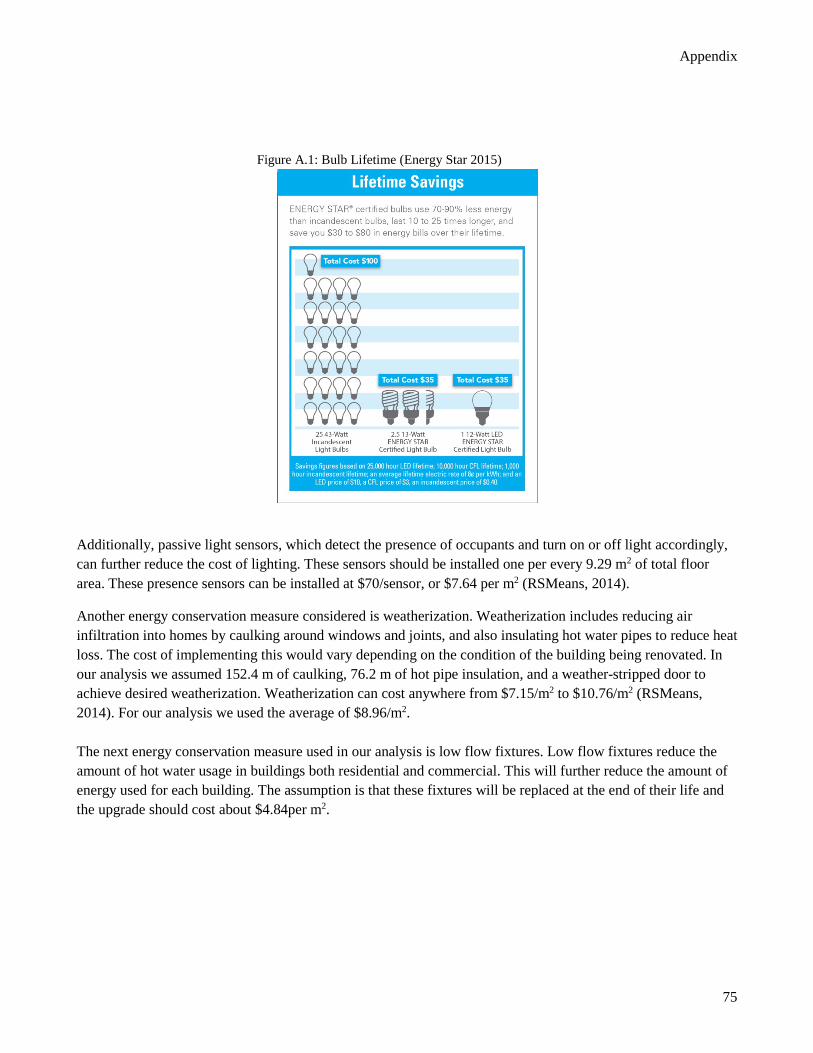
Appendix

75

Figure A.1: Bulb Lifetime (Energy Star 2015)

Additionally, passive light sensors, which detect the presence of occupants and turn on or off light accordingly, can further reduce the cost of lighting. These sensors should be installed one per every 9.29 m2 of total floor area. These presence sensors can be installed at $70/sensor, or $7.64 per m2 (RSMeans, 2014).

Another energy conservation measure considered is weatherization. Weatherization includes reducing air infiltration into homes by caulking around windows and joints, and also insulating hot water pipes to reduce heat loss. The cost of implementing this would vary depending on the condition of the building being renovated. In our analysis we assumed 152.4 m of caulking, 76.2 m of hot pipe insulation, and a weather-stripped door to achieve desired weatherization. Weatherization can cost anywhere from $7.15/m2 to $10.76/m2 (RSMeans, 2014). For our analysis we used the average of $8.96/m2. The next energy conservation measure used in our analysis is low flow fixtures. Low flow fixtures reduce the amount of hot water usage in buildings both residential and commercial. This will further reduce the amount of energy used for each building. The assumption is that these fixtures will be replaced at the end of their life and the upgrade should cost about $4.84per m2.

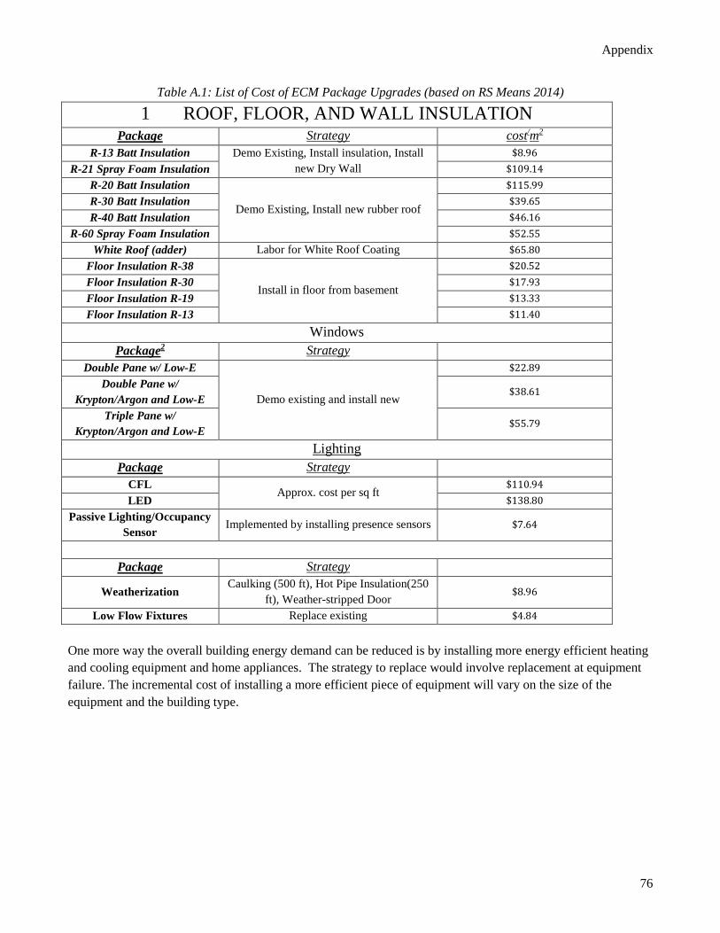
Appendix

76

Table A.1: List of Cost of ECM Package Upgrades (based on RS Means 2014)

1 ROOF, FLOOR, AND WALL INSULATION Package Strategy cost/m2

R-13 Batt Insulation Demo Existing, Install insulation, Install new Dry Wall

$8.96 R-21 Spray Foam Insulation $109.14

R-20 Batt Insulation

Demo Existing, Install new rubber roof

$115.99 R-30 Batt Insulation $39.65 R-40 Batt Insulation $46.16

R-60 Spray Foam Insulation $52.55 White Roof (adder) Labor for White Roof Coating $65.80

Floor Insulation R-38

Install in floor from basement

$20.52 Floor Insulation R-30 $17.93 Floor Insulation R-19 $13.33 Floor Insulation R-13 $11.40

Windows Package2 Strategy

Double Pane w/ Low-E

Demo existing and install new

$22.89 Double Pane w/

Krypton/Argon and Low-E $38.61

Triple Pane w/ Krypton/Argon and Low-E

$55.79

Lighting Package Strategy

CFL Approx. cost per sq ft

$110.94 LED $138.80

Passive Lighting/Occupancy Sensor

Implemented by installing presence sensors $7.64

Package Strategy

Weatherization Caulking (500 ft), Hot Pipe Insulation(250

ft), Weather-stripped Door $8.96

Low Flow Fixtures Replace existing $4.84 One more way the overall building energy demand can be reduced is by installing more energy efficient heating and cooling equipment and home appliances. The strategy to replace would involve replacement at equipment failure. The incremental cost of installing a more efficient piece of equipment will vary on the size of the equipment and the building type.

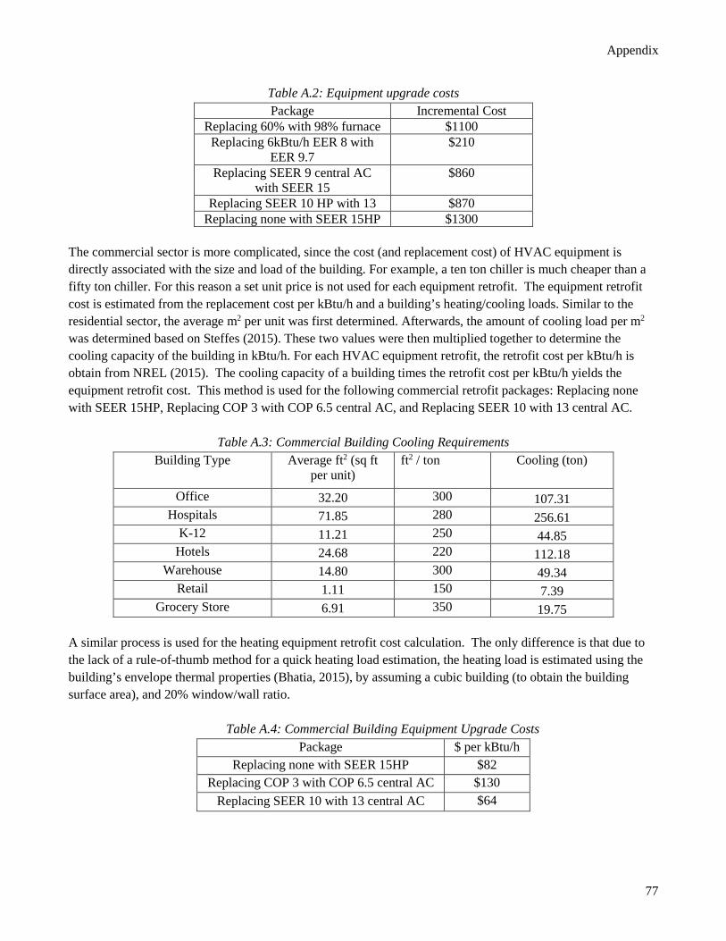
Appendix

77

Table A.2: Equipment upgrade costs Package Incremental Cost

Replacing 60% with 98% furnace $1100 Replacing 6kBtu/h EER 8 with

EER 9.7 $210

Replacing SEER 9 central AC with SEER 15

$860

Replacing SEER 10 HP with 13 $870 Replacing none with SEER 15HP $1300

The commercial sector is more complicated, since the cost (and replacement cost) of HVAC equipment is directly associated with the size and load of the building. For example, a ten ton chiller is much cheaper than a fifty ton chiller. For this reason a set unit price is not used for each equipment retrofit. The equipment retrofit cost is estimated from the replacement cost per kBtu/h and a building’s heating/cooling loads. Similar to the residential sector, the average m2 per unit was first determined. Afterwards, the amount of cooling load per m2 was determined based on Steffes (2015). These two values were then multiplied together to determine the cooling capacity of the building in kBtu/h. For each HVAC equipment retrofit, the retrofit cost per kBtu/h is obtain from NREL (2015). The cooling capacity of a building times the retrofit cost per kBtu/h yields the equipment retrofit cost. This method is used for the following commercial retrofit packages: Replacing none with SEER 15HP, Replacing COP 3 with COP 6.5 central AC, and Replacing SEER 10 with 13 central AC.

Table A.3: Commercial Building Cooling Requirements Building Type Average ft2 (sq ft

per unit) ft2 / ton Cooling (ton)

Office 32.20 300 107.31 Hospitals 71.85 280 256.61

K-12 11.21 250 44.85 Hotels 24.68 220 112.18

Warehouse 14.80 300 49.34 Retail 1.11 150 7.39

Grocery Store 6.91 350 19.75 A similar process is used for the heating equipment retrofit cost calculation. The only difference is that due to the lack of a rule-of-thumb method for a quick heating load estimation, the heating load is estimated using the building’s envelope thermal properties (Bhatia, 2015), by assuming a cubic building (to obtain the building surface area), and 20% window/wall ratio. Table A.4: Commercial Building Equipment Upgrade Costs

Package $ per kBtu/h Replacing none with SEER 15HP $82

Replacing COP 3 with COP 6.5 central AC $130 Replacing SEER 10 with 13 central AC $64

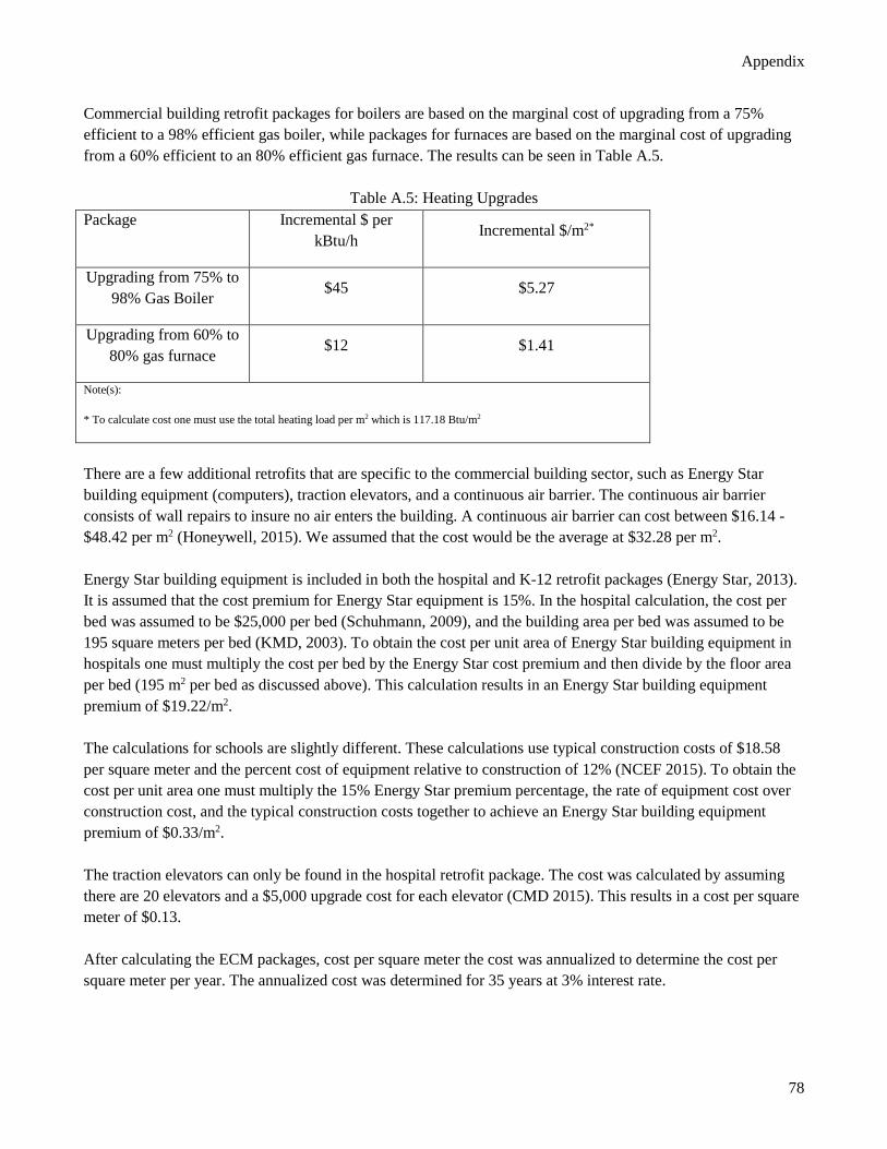
Appendix

78

Commercial building retrofit packages for boilers are based on the marginal cost of upgrading from a 75% efficient to a 98% efficient gas boiler, while packages for furnaces are based on the marginal cost of upgrading from a 60% efficient to an 80% efficient gas furnace. The results can be seen in Table A.5.

Table A.5: Heating Upgrades Package Incremental $ per

kBtu/h Incremental $/m2*

Upgrading from 75% to 98% Gas Boiler $45 $5.27

Upgrading from 60% to 80% gas furnace $12 $1.41

Note(s):

* To calculate cost one must use the total heating load per m2 which is 117.18 Btu/m2

There are a few additional retrofits that are specific to the commercial building sector, such as Energy Star building equipment (computers), traction elevators, and a continuous air barrier. The continuous air barrier consists of wall repairs to insure no air enters the building. A continuous air barrier can cost between $16.14 - $48.42 per m2 (Honeywell, 2015). We assumed that the cost would be the average at $32.28 per m2. Energy Star building equipment is included in both the hospital and K-12 retrofit packages (Energy Star, 2013). It is assumed that the cost premium for Energy Star equipment is 15%. In the hospital calculation, the cost per bed was assumed to be $25,000 per bed (Schuhmann, 2009), and the building area per bed was assumed to be 195 square meters per bed (KMD, 2003). To obtain the cost per unit area of Energy Star building equipment in hospitals one must multiply the cost per bed by the Energy Star cost premium and then divide by the floor area per bed (195 m2 per bed as discussed above). This calculation results in an Energy Star building equipment premium of $19.22/m2. The calculations for schools are slightly different. These calculations use typical construction costs of $18.58 per square meter and the percent cost of equipment relative to construction of 12% (NCEF 2015). To obtain the cost per unit area one must multiply the 15% Energy Star premium percentage, the rate of equipment cost over construction cost, and the typical construction costs together to achieve an Energy Star building equipment premium of $0.33/m2. The traction elevators can only be found in the hospital retrofit package. The cost was calculated by assuming there are 20 elevators and a $5,000 upgrade cost for each elevator (CMD 2015). This results in a cost per square meter of $0.13. After calculating the ECM packages, cost per square meter the cost was annualized to determine the cost per square meter per year. The annualized cost was determined for 35 years at 3% interest rate.

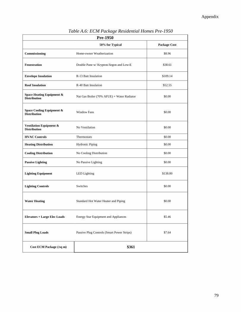
Appendix

79

Table A.6: ECM Package Residential Homes Pre-1950 Pre-1950

50% for Typical Package Cost

Commissioning Home-owner Weatherization $8.96

Fenestration Double Pane w/ Krypton/Argon and Low-E $38.61

Envelope Insulation R-13 Batt Insulation $109.14

Roof Insulation R-40 Batt Insulation $52.55

Space Heating Equipment & Distribution Nat Gas Boiler (70% AFUE) + Water Radiator $0.00

Space Cooling Equipment & Distribution Window Fans $0.00

Ventilation Equipment & Distribution No Ventilation $0.00

HVAC Controls Thermostats $0.00

Heating Distribution Hydronic Piping $0.00

Cooling Distribution No Cooling Distribution $0.00

Passive Lighting No Passive Lighting $0.00

Lighting Equipment LED Lighting $138.80

Lighting Controls Switches $0.00

Water Heating Standard Hot Water Heater and Piping $0.00

Elevators + Large Elec Loads Energy Star Equipment and Appliances $5.46

Small Plug Loads Passive Plug Controls (Smart Power Strips) $7.64

Cost ECM Package (/sq m) $361

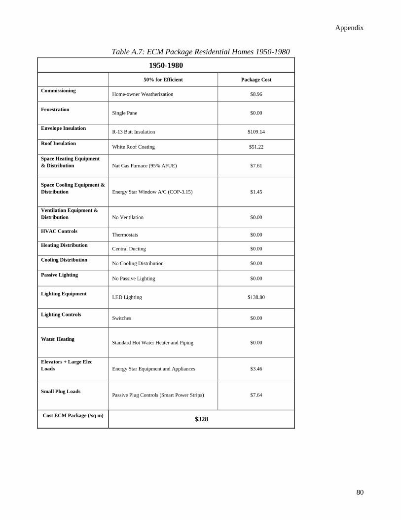
Appendix

80

Table A.7: ECM Package Residential Homes 1950-1980

1950-1980

50% for Efficient Package Cost

Commissioning Home-owner Weatherization $8.96

Fenestration Single Pane $0.00

Envelope Insulation R-13 Batt Insulation $109.14

Roof Insulation White Roof Coating $51.22

Space Heating Equipment & Distribution Nat Gas Furnace (95% AFUE) $7.61

Space Cooling Equipment & Distribution Energy Star Window A/C (COP-3.15) $1.45

Ventilation Equipment & Distribution No Ventilation $0.00

HVAC Controls Thermostats $0.00

Heating Distribution Central Ducting $0.00

Cooling Distribution No Cooling Distribution $0.00

Passive Lighting No Passive Lighting $0.00

Lighting Equipment LED Lighting $138.80

Lighting Controls Switches $0.00

Water Heating Standard Hot Water Heater and Piping $0.00

Elevators + Large Elec Loads Energy Star Equipment and Appliances $3.46

Small Plug Loads Passive Plug Controls (Smart Power Strips) $7.64

Cost ECM Package (/sq m) $328

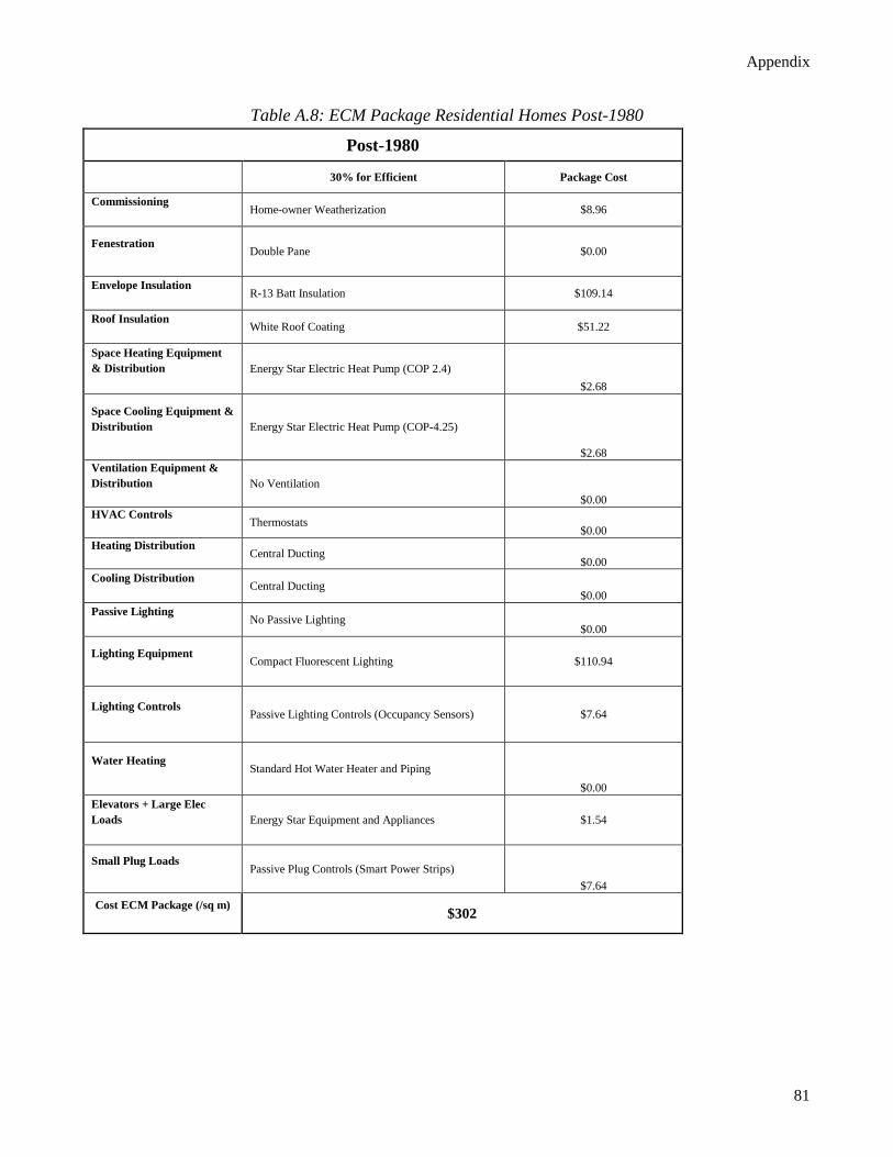
Appendix

81

Table A.8: ECM Package Residential Homes Post-1980

Post-1980

30% for Efficient Package Cost

Commissioning Home-owner Weatherization $8.96

Fenestration Double Pane $0.00

Envelope Insulation R-13 Batt Insulation $109.14

Roof Insulation White Roof Coating $51.22

Space Heating Equipment & Distribution Energy Star Electric Heat Pump (COP 2.4)

$2.68

Space Cooling Equipment & Distribution Energy Star Electric Heat Pump (COP-4.25)

$2.68 Ventilation Equipment & Distribution No Ventilation

$0.00 HVAC Controls

Thermostats $0.00

Heating Distribution Central Ducting

$0.00 Cooling Distribution

Central Ducting $0.00

Passive Lighting No Passive Lighting

$0.00

Lighting Equipment Compact Fluorescent Lighting $110.94

Lighting Controls Passive Lighting Controls (Occupancy Sensors) $7.64

Water Heating Standard Hot Water Heater and Piping

$0.00 Elevators + Large Elec Loads Energy Star Equipment and Appliances $1.54

Small Plug Loads Passive Plug Controls (Smart Power Strips)

$7.64 Cost ECM Package (/sq m) $302

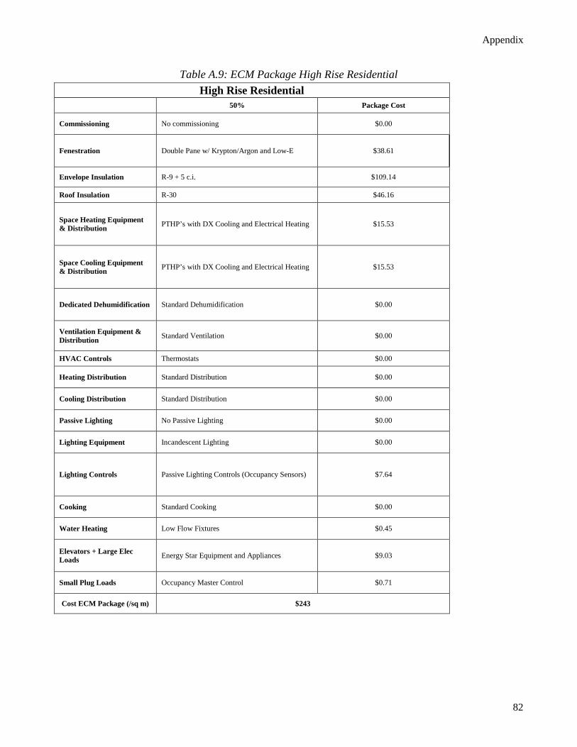
Appendix

82

Table A.9: ECM Package High Rise Residential High Rise Residential

50% Package Cost

Commissioning No commissioning $0.00

Fenestration Double Pane w/ Krypton/Argon and Low-E $38.61

Envelope Insulation R-9 + 5 c.i. $109.14

Roof Insulation R-30 $46.16

Space Heating Equipment & Distribution PTHP’s with DX Cooling and Electrical Heating $15.53

Space Cooling Equipment & Distribution PTHP’s with DX Cooling and Electrical Heating $15.53

Dedicated Dehumidification Standard Dehumidification $0.00

Ventilation Equipment & Distribution Standard Ventilation $0.00

HVAC Controls Thermostats $0.00

Heating Distribution Standard Distribution $0.00

Cooling Distribution Standard Distribution $0.00

Passive Lighting No Passive Lighting $0.00

Lighting Equipment Incandescent Lighting $0.00

Lighting Controls Passive Lighting Controls (Occupancy Sensors) $7.64

Cooking Standard Cooking $0.00

Water Heating Low Flow Fixtures $0.45

Elevators + Large Elec Loads Energy Star Equipment and Appliances $9.03

Small Plug Loads Occupancy Master Control $0.71

Cost ECM Package (/sq m) $243

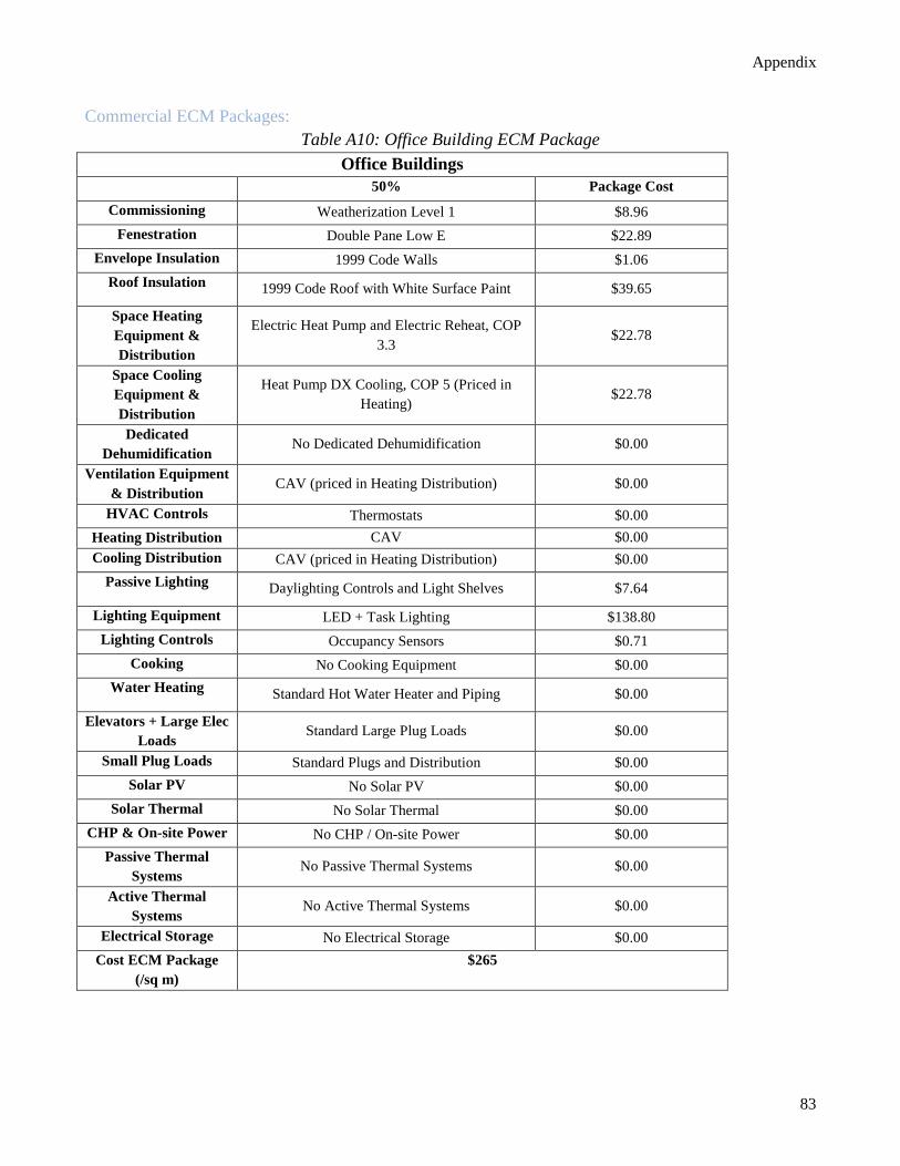
Appendix

83

Commercial ECM Packages: Table A10: Office Building ECM Package

Office Buildings 50% Package Cost

Commissioning Weatherization Level 1 $8.96 Fenestration Double Pane Low E $22.89

Envelope Insulation 1999 Code Walls $1.06 Roof Insulation 1999 Code Roof with White Surface Paint $39.65

Space Heating Equipment & Distribution

Electric Heat Pump and Electric Reheat, COP 3.3

$22.78

Space Cooling Equipment & Distribution

Heat Pump DX Cooling, COP 5 (Priced in Heating)

$22.78

Dedicated Dehumidification

No Dedicated Dehumidification $0.00

Ventilation Equipment & Distribution

CAV (priced in Heating Distribution) $0.00

HVAC Controls Thermostats $0.00 Heating Distribution CAV $0.00 Cooling Distribution CAV (priced in Heating Distribution) $0.00

Passive Lighting Daylighting Controls and Light Shelves $7.64

Lighting Equipment LED + Task Lighting $138.80 Lighting Controls Occupancy Sensors $0.71

Cooking No Cooking Equipment $0.00 Water Heating Standard Hot Water Heater and Piping $0.00

Elevators + Large Elec Loads

Standard Large Plug Loads $0.00

Small Plug Loads Standard Plugs and Distribution $0.00 Solar PV No Solar PV $0.00

Solar Thermal No Solar Thermal $0.00 CHP & On-site Power No CHP / On-site Power $0.00

Passive Thermal Systems

No Passive Thermal Systems $0.00

Active Thermal Systems

No Active Thermal Systems $0.00

Electrical Storage No Electrical Storage $0.00 Cost ECM Package

(/sq m) $265

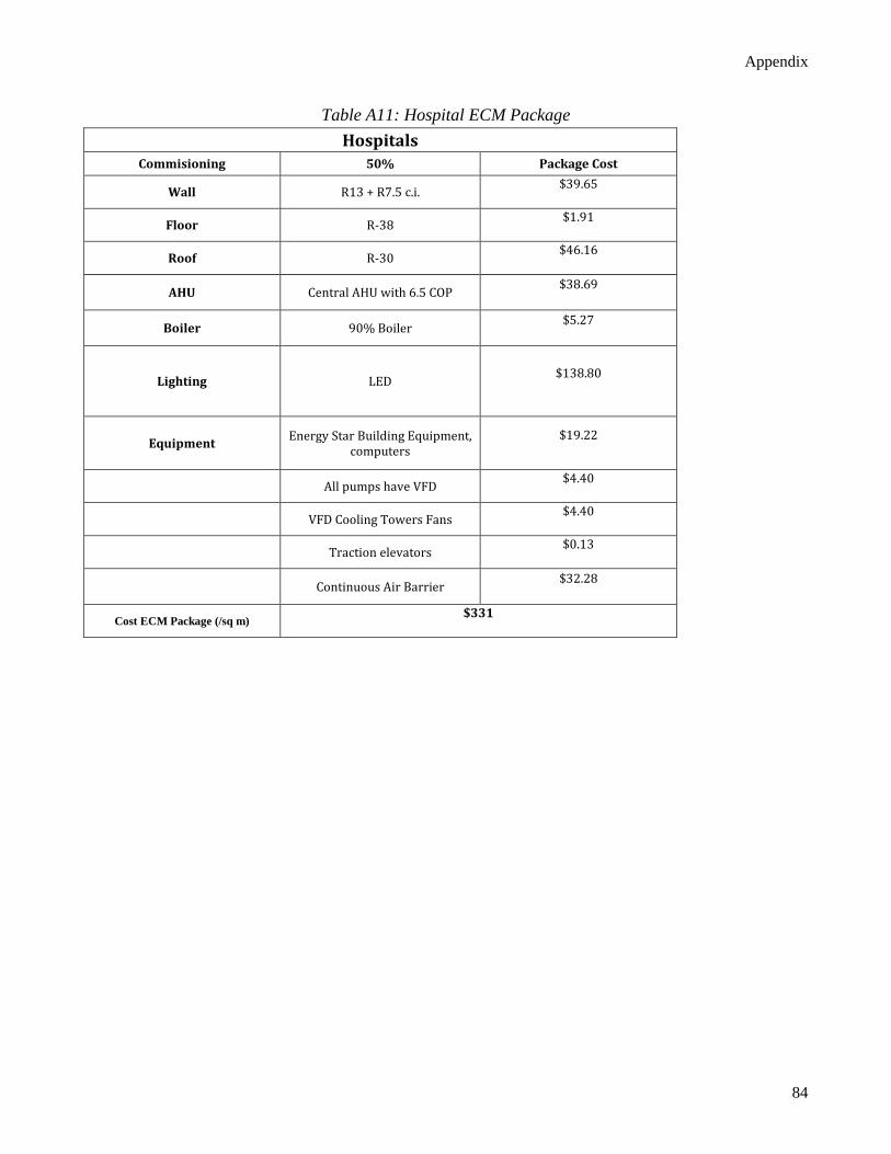
Appendix

84

Table A11: Hospital ECM Package Hospitals

Commisioning 50% Package Cost

Wall R13 + R7.5 c.i. $39.65

Floor R-38 $1.91

Roof R-30 $46.16

AHU Central AHU with 6.5 COP $38.69

Boiler 90% Boiler $5.27

Lighting LED $138.80

Equipment Energy Star Building Equipment, computers

$19.22

All pumps have VFD $4.40

VFD Cooling Towers Fans $4.40

Traction elevators $0.13

Continuous Air Barrier $32.28

Cost ECM Package (/sq m) $331

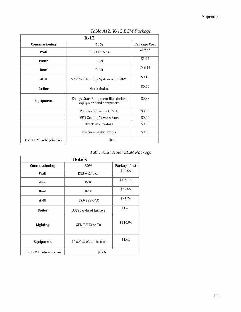
Appendix

85

Table A12: K-12 ECM Package K-12

Commissioning 50% Package Cost

Wall R13 + R7.5 c.i. $39.65

Floor R-38 $1.91

Roof R-30 $46.16

AHU VAV Air-Handling System with DOAS $0.10

Boiler Not included $0.00

Equipment Energy Start Equipment like kitchen equipment and computers

$0.33

Pumps and fans with VFD $0.00

VFD Cooling Towers Fans $0.00

Traction elevators $0.00

Continuous Air Barrier $0.00

Cost ECM Package (/sq m) $88

Table A13: Hotel ECM Package

Hotels Commissioning 30% Package Cost

Wall R13 + R7.5 c.i. $39.65

Floor R-10 $109.14

Roof R-20 $39.65

AHU 13.0 SEER AC $24.24

Boiler 80% gas-fired furnace $1.41

Lighting CFL, T5HO or T8 $110.94

Equipment 90% Gas Water heater $1.41

Cost ECM Package (/sq m) $326

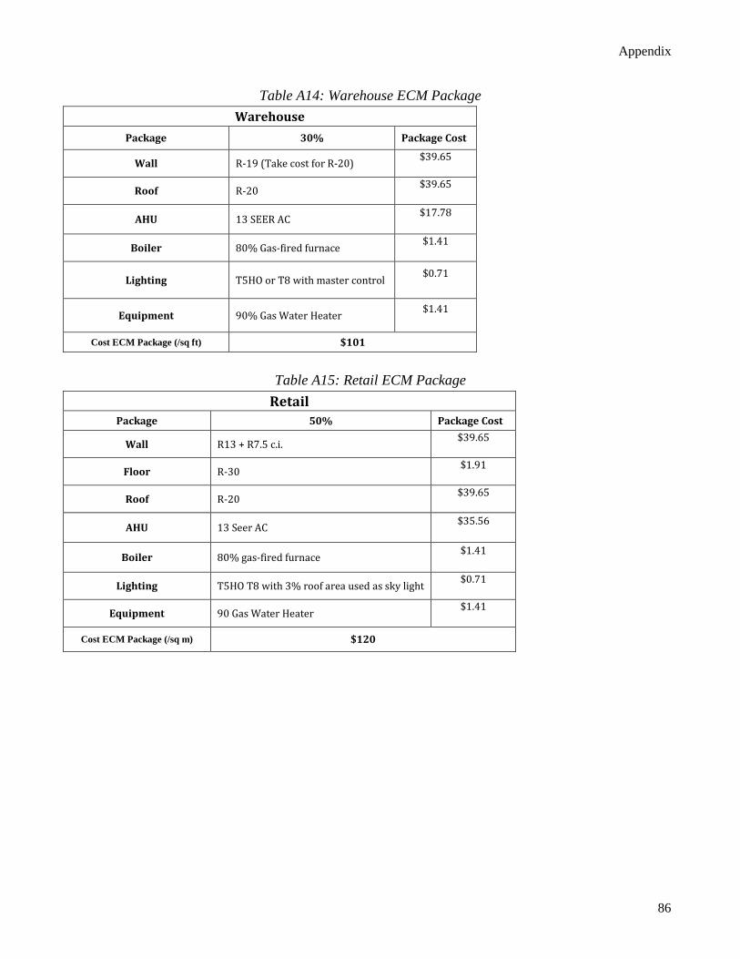
Appendix

86

Table A14: Warehouse ECM Package Warehouse

Package 30% Package Cost

Wall R-19 (Take cost for R-20) $39.65

Roof R-20 $39.65

AHU 13 SEER AC $17.78

Boiler 80% Gas-fired furnace $1.41

Lighting T5HO or T8 with master control $0.71

Equipment 90% Gas Water Heater $1.41

Cost ECM Package (/sq ft) $101

Table A15: Retail ECM Package

Retail Package 50% Package Cost

Wall R13 + R7.5 c.i. $39.65

Floor R-30 $1.91

Roof R-20 $39.65

AHU 13 Seer AC $35.56

Boiler 80% gas-fired furnace $1.41

Lighting T5HO T8 with 3% roof area used as sky light $0.71

Equipment 90 Gas Water Heater $1.41

Cost ECM Package (/sq m) $120

Appendix

87

Table A16: Grocery Store ECM Package Grocery Store

Package 50% Package Cost

Wall R13 + R7.5 c.i. $39.65

Floor R-30 $1.91

Roof R-30 $46.16

Boiler MA SZVAV DC Package RTU $0.00

Lighting ALL LED Lighting with occupancy master control $1.41

Equipment 94% Gas Water Heater $138.80

Continuous Air Barrier $32.28

Cost ECM Package (/sq ft) $262

Appendix

88

9 APPENDIX B 9.1 Climate Policy Approaches by City

This appendix summarizes a review of the climate change policy approaches of ten U.S. cities. The climate change policy apparatus is first described and then categorized as mainstreaming vs. dedicated and governmental action vs. public private partnership action.

City Office/Position Climate Change Project

New York, NY Mayor’s Office of Long-term

Planning &Sustainability Mayor’s Office of Long-term

Planning & Sustainability New York City has an ambitious climate change effort, including a commitment to reducing GHG emissions 80% from 2005 by 2050 (NYC 2014a). As of 2013 emissions had been reduced 19% from the 2005 baseline largely through fuel switching to natural gas for electricity generation and building heating (NYC 2014b).

New York’s climate change efforts are led by the Mayor’s Office of Long-term Planning & Sustainability. While the mission of this office is to “Improve New York City’s quality of life, environmental sustainability, and resilience to climate change by developing plans and programs based on rigorous analysis and measurable action steps” ("Office of Environmental Quality," 2015), and therefore may appear to be reflect a dedicated approach, the office is actually structured within the bounds of mainstreaming. It is partnered with more than 15 city agencies (Bloomberg, 2006) to “develop and oversee implementation of PlaNYC, the City’s integrated sustainability plan for a greener, greater New York, and related Mayoral interagency initiatives” ("Office of Environmental Quality," 2015). The Mayor’s Office of Long-term Planning & Sustainability works with other city agencies to devise these “interagency initiatives.” The authority to act on climate change in the policy implementation process appears to be diffuse and horizontally integrated among various relevant actors within the city. “[I]ndependent scientists, think tank scholars, respected academics and city planners, and innovative green builders… neighborhood activists, public interest advocates, labor leaders, and others from the private and non-profit sectors” focus on “community-based strategic planning, not central planning,” to craft New York City’s response to climate change (Bloomberg, 2006). It is therefore reasonable to conclude that the New York is a mainstreaming/public private partnership action city.

City Office/Position Climate Change Project Chicago, IL Chief Sustainability Officer Sustainable Chicago

Chicago’s climate change policy efforts were initiated in 2008 under Mayor Richard M. Daley, who appointed a Climate Task Force with the goal of developing a plan for significant and achievable reductions in the city’s greenhouse gas emissions. This effort identified twenty-six mitigation or emissions reduction actions. An overall goal was set of achieving an 80 percent reduction below 1990 GHG emissions level by the year 2050 (Chicago, 2008). In 2011, Rahm Emanuel was elected as mayor, and the City drafted the Sustainable Chicago plan which outlined 24 goals with a much shorter time horizon of 2015. The goal by 2015 is to improve citywide efficiency by 5 percent, and create at least an additional 20 MW of renewable energy. The 6 month progress report of Sustainable Chicago plan notes that the city has proactively made concrete progress on 22 or the 24 goals initially outlined (Chicago, 2015).

Appendix

89

Underlying these different efforts is a transition in Chicago’s response to the issue of climate change. Chicago had once been a model for a dedicated/governmental action city. Under Mayor Richard M. Daley, all of the city’s efforts to mitigate and/or adapt to climate change came out of the Department of Environment. When current Mayor Rahm Emanuel took office in 2011, however, one of his first acts in office was to appoint a Chief Sustainability Officer (CSO) and disband the Department of Environment (Nemes, 2011). The Department of Environment staff that remained after the restructuring were moved to the city’s General Services, Transportation, and Public Health Departments, in what the City’s CSO dubbed a “a strategic move to elevate and embed sustainability into everything we do in the city of Chicago” (Nemes, 2011). This is a very clear-cut example of a city’s transition from a dedicated to mainstreaming governmental structure for climate change action. But while Chicago seems to have made that transition well, it is appears to be less enthusiastically pursuing a shift from governmental action style of policy implementation to that of public private partnership action. For example, the Chicago Sustainability Council, which oversees Sustainable Chicago and publishes its progress reports, is entirely comprised of municipal government staff. On the other hand, the city is also actively working to “[r]ecruit companies and individuals with the most innovative clean energy and sustainability solutions to Chicago” (Chicago, 2012), ostensibly to share in the responsibility of creating and implementing the policies housed within the Sustainable Chicago plan. What remains unclear, however, is how fully these non-governmental entities will actually be integrated into climate change policy planning and implementation. For these reasons, it is appropriate to consider Chicago a mainstreaming/governmental action city.

City Office/Position Climate Change Project

Houston, TX Office of Sustainability / Director of Sustainability

Green Houston

Houston has a longstanding climate change mitigation effort. The city developed an emissions reduction plan as early as the year 2000 and updated the plan in the year 2005. In 2008, the City drafted a new Multi-Pollutant Emission Reduction Plan (MERP) which outlined emissions targets for 2010 and strategies to achieve these goals. This report uses 2005 as the baseline year. Then the emissions of each pollutant for each source category were calculated. Pollutants targeted in the report were greenhouse gases, nitrogen oxides, and volatile organic compounds. The 2010 goals are conservative because they are “based solely on readily quantifiable emission reductions attributable to strategies developed through mid-2008.” (Houston, 2008). In 2009 Houston produced an update to this 2008 MERP plan which addresses fourteen additional strategies implemented by the City to assist with reaching the emissions reduction goals. (Houston, 2009). Currently, the City of Houston is working with Houston Advanced Research Center (HARC) on an updated city-wide Sustainable Action Plan. This plan will provide updated strategies to continue the City’s energy efficiency and renewable energy programs as well as incorporate additional mitigation and adaptation strategies (HARC, 2015)

Houston’s city government has a rather unique approach for how it is structured to act on climate change. In one way, Houston employs the dedicated approach to climate change action within government in that the mayor appoints a sustainability director who is a member of the mayor’s staff and is “responsible for directing and coordinating projects and initiatives that improve air, land and water quality; and support and expand renewable energy, energy efficiency, green buildings, recycling and composting, alternative and clean transportation, local food production and more livable and vibrant neighborhoods” (City of Houston, 2015). But it would be inaccurate to label Houston’s municipal climate change structure as simply dedicated. Running parallel to the dedicated, executive-led sustainability efforts mentioned above is the existence of an Environmental

Appendix

90

Coordinating Council (ECC), which embodies the principles of the mainstreaming approach. The ECC is comprised of city employees from each of the city’s departments, and is tasked with “coordinating environmental investigations and enforcement work across departments… enhancing cross-departmental environmental education… [and] coordinating communications regarding environmental matters” ("Environmental Coordinating Council," 2015). Of the ten cities examined here, Houston is the only one that houses two parallel governmental structures for dealing with climate change, each of which serves as a prime example of its corresponding theoretical models. It would not be unfair to say that Houston is therefore utilizing both the dedicated approach and the mainstreaming approach to government action on climate change.

Houston’s climate change policy implementation apparatus, however, falls much more neatly into one camp. As opposed to one comprehensive project, Green Houston is actually series of smaller, actionable initiatives, generally led by “volunteers” within a number of different municipal departments ("Climate Change," 2015). While one of these initiatives, the “Green Office Challenge,” seems to meet the criteria for public private partnership action—in that it relies on the cooperation of governmental and nongovernmental actors, each operating in their respective fields, in order to meet its goal of more energy and resource efficient commercial property ("Climate Change: Programs & Policies," 2015)—it is nonetheless difficult to make the case that Houston employs a public private partnership action policy implementation apparatus, given that most of Green Houston’s other initiatives are government-generated. A possible explanation for the general lack of involvement in climate change policy implementation by nongovernmental city actors is that Houston is home to “more than 5,000 energy related firms” ("Houston Facts and Figures," 2015), most of which are unlikely to support any effort to wean society off fossil fuel reliance. Thus, the city of Houston’s approach is characterized as having a dedicated & mainstream/governmental action structure.

City Office/Position Climate Change Project

Phoenix, AZ Office of Environmental Programs; Environmental

Quality Commission

Climate Action Plan – SustainPHX

The City of Phoenix developed a Climate Action Plan in 2009 which identified methods to reduce GHG emissions from city operations to 5% the 2005 levels. By 2012, the city had already reduced emissions to 7.2% below the 2005 levels (678,150 to 629,504 metric tons CO2e) as indicated in the 2012 Greenhouse Gas Emissions Reduction Report (Sustainable Solution Services, 2013). Subsequently, the city has adopted a more recent goal to reduce greenhouse gas (GHG) emissions from city operations to 15% by 2015 (City of Phoenix, 2015).

Phoenix is the first council-manager system of municipal government in our comparison. As such, a city manager runs the daily operations of the city and heads the city’s executive branch of government ("How the City Works," 2015). Under the city manager are a number of deputy managers and assistants who are each responsible for various city activities ("City Organizational Chart," 2015). The deputy city manager in charge of the Office of Environmental Programs (OEP) also oversees water services, public transit, and planning & development operations ("Deputy City Manager Rick Naimark," 2015). This municipal system of government lends itself to the mainstreaming approach. By consolidating separate city spheres of operations under the direction of one person, this person can, in principle, structure operations so as to weave consideration of climate change action into the fabric of many types of city operations.

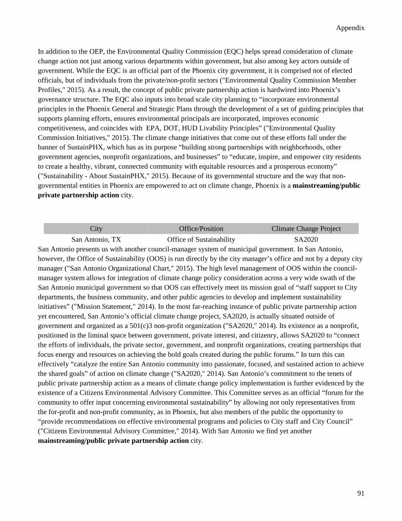
Appendix

91

In addition to the OEP, the Environmental Quality Commission (EQC) helps spread consideration of climate change action not just among various departments within government, but also among key actors outside of government. While the EQC is an official part of the Phoenix city government, it is comprised not of elected officials, but of individuals from the private/non-profit sectors ("Environmental Quality Commission Member Profiles," 2015). As a result, the concept of public private partnership action is hardwired into Phoenix’s governance structure. The EQC also inputs into broad scale city planning to “incorporate environmental principles in the Phoenix General and Strategic Plans through the development of a set of guiding principles that supports planning efforts, ensures environmental principals are incorporated, improves economic competitiveness, and coincides with EPA, DOT, HUD Livability Principles” ("Environmental Quality Commission Initiatives," 2015). The climate change initiatives that come out of these efforts fall under the banner of SustainPHX, which has as its purpose “building strong partnerships with neighborhoods, other government agencies, nonprofit organizations, and businesses” to “educate, inspire, and empower city residents to create a healthy, vibrant, connected community with equitable resources and a prosperous economy” ("Sustainability - About SustainPHX," 2015). Because of its governmental structure and the way that non-governmental entities in Phoenix are empowered to act on climate change, Phoenix is a mainstreaming/public private partnership action city.

City Office/Position Climate Change Project San Antonio, TX Office of Sustainability SA2020

San Antonio presents us with another council-manager system of municipal government. In San Antonio, however, the Office of Sustainability (OOS) is run directly by the city manager’s office and not by a deputy city manager ("San Antonio Organizational Chart," 2015). The high level management of OOS within the council-manager system allows for integration of climate change policy consideration across a very wide swath of the San Antonio municipal government so that OOS can effectively meet its mission goal of “staff support to City departments, the business community, and other public agencies to develop and implement sustainability initiatives” ("Mission Statement," 2014). In the most far-reaching instance of public private partnership action yet encountered, San Antonio’s official climate change project, SA2020, is actually situated outside of government and organized as a 501(c)3 non-profit organization ("SA2020," 2014). Its existence as a nonprofit, positioned in the liminal space between government, private interest, and citizenry, allows SA2020 to “connect the efforts of individuals, the private sector, government, and nonprofit organizations, creating partnerships that focus energy and resources on achieving the bold goals created during the public forums.” In turn this can effectively “catalyze the entire San Antonio community into passionate, focused, and sustained action to achieve the shared goals” of action on climate change ("SA2020," 2014). San Antonio’s commitment to the tenets of public private partnership action as a means of climate change policy implementation is further evidenced by the existence of a Citizens Environmental Advisory Committee. This Committee serves as an official “forum for the community to offer input concerning environmental sustainability” by allowing not only representatives from the for-profit and non-profit community, as in Phoenix, but also members of the public the opportunity to “provide recommendations on effective environmental programs and policies to City staff and City Council” ("Citizens Environmental Advisory Committee," 2014). With San Antonio we find yet another mainstreaming/public private partnership action city.

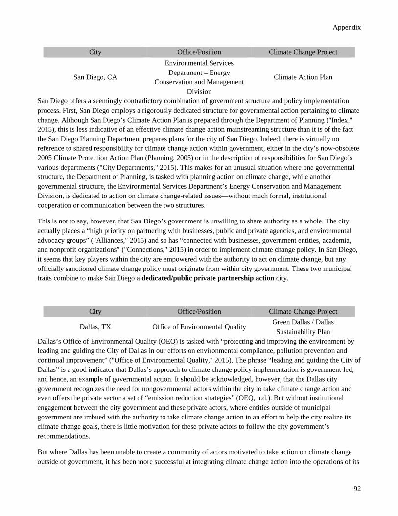
Appendix

92

City Office/Position Climate Change Project

San Diego, CA

Environmental Services Department – Energy

Conservation and Management Division

Climate Action Plan

San Diego offers a seemingly contradictory combination of government structure and policy implementation process. First, San Diego employs a rigorously dedicated structure for governmental action pertaining to climate change. Although San Diego’s Climate Action Plan is prepared through the Department of Planning ("Index," 2015), this is less indicative of an effective climate change action mainstreaming structure than it is of the fact the San Diego Planning Department prepares plans for the city of San Diego. Indeed, there is virtually no reference to shared responsibility for climate change action within government, either in the city’s now-obsolete 2005 Climate Protection Action Plan (Planning, 2005) or in the description of responsibilities for San Diego’s various departments ("City Departments," 2015). This makes for an unusual situation where one governmental structure, the Department of Planning, is tasked with planning action on climate change, while another governmental structure, the Environmental Services Department’s Energy Conservation and Management Division, is dedicated to action on climate change-related issues—without much formal, institutional cooperation or communication between the two structures.

This is not to say, however, that San Diego’s government is unwilling to share authority as a whole. The city actually places a “high priority on partnering with businesses, public and private agencies, and environmental advocacy groups” ("Alliances," 2015) and so has “connected with businesses, government entities, academia, and nonprofit organizations” ("Connections," 2015) in order to implement climate change policy. In San Diego, it seems that key players within the city are empowered with the authority to act on climate change, but any officially sanctioned climate change policy must originate from within city government. These two municipal traits combine to make San Diego a dedicated/public private partnership action city.

City Office/Position Climate Change Project

Dallas, TX Office of Environmental Quality Green Dallas / Dallas Sustainability Plan

Dallas’s Office of Environmental Quality (OEQ) is tasked with “protecting and improving the environment by leading and guiding the City of Dallas in our efforts on environmental compliance, pollution prevention and continual improvement” ("Office of Environmental Quality," 2015). The phrase “leading and guiding the City of Dallas” is a good indicator that Dallas’s approach to climate change policy implementation is government-led, and hence, an example of governmental action. It should be acknowledged, however, that the Dallas city government recognizes the need for nongovernmental actors within the city to take climate change action and even offers the private sector a set of “emission reduction strategies” (OEQ, n.d.). But without institutional engagement between the city government and these private actors, where entities outside of municipal government are imbued with the authority to take climate change action in an effort to help the city realize its climate change goals, there is little motivation for these private actors to follow the city government’s recommendations.

But where Dallas has been unable to create a community of actors motivated to take action on climate change outside of government, it has been more successful at integrating climate change action into the operations of its

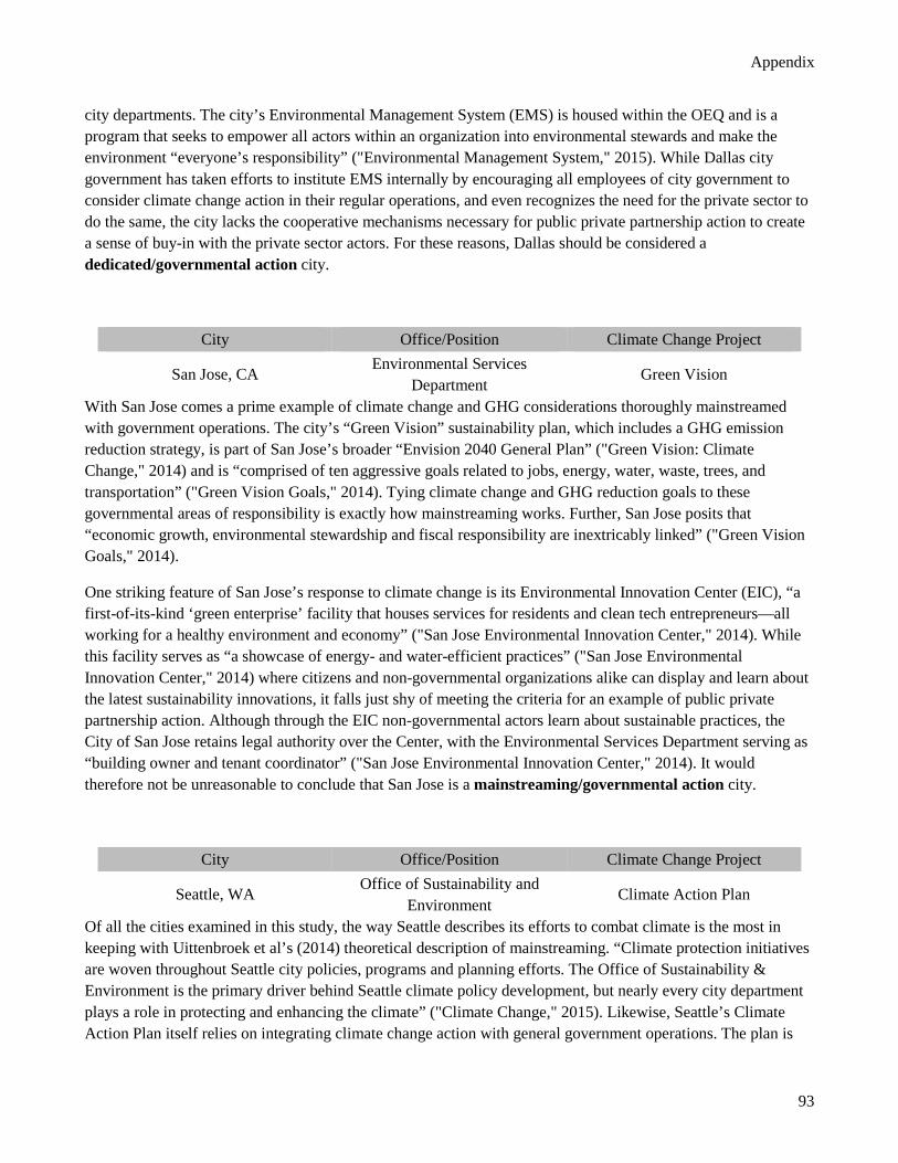
Appendix

93

city departments. The city’s Environmental Management System (EMS) is housed within the OEQ and is a program that seeks to empower all actors within an organization into environmental stewards and make the environment “everyone’s responsibility” ("Environmental Management System," 2015). While Dallas city government has taken efforts to institute EMS internally by encouraging all employees of city government to consider climate change action in their regular operations, and even recognizes the need for the private sector to do the same, the city lacks the cooperative mechanisms necessary for public private partnership action to create a sense of buy-in with the private sector actors. For these reasons, Dallas should be considered a dedicated/governmental action city.

City Office/Position Climate Change Project

San Jose, CA Environmental Services Department

Green Vision

With San Jose comes a prime example of climate change and GHG considerations thoroughly mainstreamed with government operations. The city’s “Green Vision” sustainability plan, which includes a GHG emission reduction strategy, is part of San Jose’s broader “Envision 2040 General Plan” ("Green Vision: Climate Change," 2014) and is “comprised of ten aggressive goals related to jobs, energy, water, waste, trees, and transportation” ("Green Vision Goals," 2014). Tying climate change and GHG reduction goals to these governmental areas of responsibility is exactly how mainstreaming works. Further, San Jose posits that “economic growth, environmental stewardship and fiscal responsibility are inextricably linked” ("Green Vision Goals," 2014).

One striking feature of San Jose’s response to climate change is its Environmental Innovation Center (EIC), “a first-of-its-kind ‘green enterprise’ facility that houses services for residents and clean tech entrepreneurs—all working for a healthy environment and economy” ("San Jose Environmental Innovation Center," 2014). While this facility serves as “a showcase of energy- and water-efficient practices” ("San Jose Environmental Innovation Center," 2014) where citizens and non-governmental organizations alike can display and learn about the latest sustainability innovations, it falls just shy of meeting the criteria for an example of public private partnership action. Although through the EIC non-governmental actors learn about sustainable practices, the City of San Jose retains legal authority over the Center, with the Environmental Services Department serving as “building owner and tenant coordinator” ("San Jose Environmental Innovation Center," 2014). It would therefore not be unreasonable to conclude that San Jose is a mainstreaming/governmental action city.

City Office/Position Climate Change Project

Seattle, WA Office of Sustainability and Environment

Climate Action Plan

Of all the cities examined in this study, the way Seattle describes its efforts to combat climate is the most in keeping with Uittenbroek et al’s (2014) theoretical description of mainstreaming. “Climate protection initiatives are woven throughout Seattle city policies, programs and planning efforts. The Office of Sustainability & Environment is the primary driver behind Seattle climate policy development, but nearly every city department plays a role in protecting and enhancing the climate” ("Climate Change," 2015). Likewise, Seattle’s Climate Action Plan itself relies on integrating climate change action with general government operations. The plan is

Appendix

94

“not a stand-alone plan. With focus areas of transportation/land use, building energy and waste, the actions identified in the Seattle Climate Action Plan are being implemented across multiple City departments” ("Climate Change: Programs & Policies," 2015).

Both San Jose and Seattle very clearly fall within the bounds of a mainstreaming governmental structure with respect to climate change consideration. Where these cities differ, however, is in the policy implementation process. Where the San Jose city government specifically coordinates the projects that unfold in the EIC, Seattle seems to more liberally empower non-governmental entities to act independently in support of the city’s sustainability goals. “Recognizing that there is no shortage of community ingenuity or ability to inspire action, but that there is often a shortage of resources, the City supports community driven climate action through grants and contracts” (OSE, 2013). By using these grants and contracts, Seattle city government does not have to expend resources to coordinate the implementation of policies for different non-governmental entities across a variety of sectors. Instead, Seattle simply funds those private projects which serve to further the city’s overall sustainability goals.

Seattle’s explicit efforts to integrate sustainability practices with general government operations and its ability to empower non-governmental actors to implement climate change policies combine to make Seattle a mainstreaming/public private partnership action city.

City Office/Position Climate Change Project Philadelphia, PA Department of Sustainability Greenworks

Philadelphia employs a mayor-council system, with the mayor elected every four years, separately from the council, and the city council itself comprised of representatives from ten council districts, plus seven at-large council members elected city-wide (Charter, 1951). The mayor, however, may appoint and approve all city department and agency heads (Charter, 1951). This form of government gives the mayor considerable latitude in forging a governing coalition from among the city’s major interest groups and in championing the particular issues or causes that appeal to members of that coalition (McGovern, 2009).

The concepts of climate change mitigation and sustainability were essentially absent from Philadelphia city government until Michael Nutter was sworn in as Mayor in 2008 (McGovern, 2009). Early on in his administration Nutter created the Mayor’s Office of Sustainability (MOS) and appointed a Director of Sustainability (City of Philadelphia, 2015). Much as in New York, these early actions on climate change represented a dedicated approach to government action on climate change, where a popularly elected political leader trumpeted the issue and placed it on the political agenda. Targets of reducing both municipal government and city-wide emissions 20% below 1990 levels by 2015 were set. While the initial organizational efforts were characteristic of a dedicated approach, MOS staff, however, quickly began to mainstream climate change action goals into city departmental operations. As opposed to the MOS rolling out climate change policies for other city departments to implement, the Director of Sustainability, serving largely in a supporting role, empowered departments to design their own policies. For example, the Director of Sustainability initiated an inter-departmental working group with high-ranking leadership from twelve city departments to help them find effective ways to integrate climate change goals—and specifically GHG emission reduction—in their day-to-day operations (personal interview). GHG reduction was framed in the context of finding ways for city departments to protect urban infrastructure and to improve “common sense efficiency” in government (personal

Appendix

95

interview). Philadelphia voters rewarded this transition toward mainstreaming and public private partnership action around urban sustainability and resilience by approving a 2014 ballot measure to create a permanent Department of Sustainability (DOS). By 2012 city-wide emissions had been reduced 1%, and by 2013 municipal government’s emissions had been reduced by 15% (Mayor’s Office of Sustainability, 2015a). Switching electricity generation sources from coal to natural gas and renewables played a role in achieving these reductions as did a program of energy efficiency in city-owned buildings which reduced energy consumption from 2006 levels by 12% by 2013 (Mayor’s Office of Sustainability, 2015a).

Appendix

96

10 APPENDIX C 10.1 Example Analysis of Impacts of Externalities and Uncertainties on Wind

Electricity Generation In determining the costs associated with implementing the low carbon energy scenarios developed in Section 4.6 of Chapter 4, there are many variables that must be accounted for, including the cost of fossil fuels, government subsidies for renewables, estimations of external savings, efficiency of wind turbines, and many other factors. The analysis in Section 4.6 of Chapter 4 did not consider externalities or variability in costs. While it was not feasible within the scope of the study to consider these effects for all electricity sources, an example analysis is conducted here for wind energy.

The Lazard (2014) study provides a range of costs for onshore wind energy from $37 to $81 per MWh, as well as an average cost for offshore wind energy of $162 per MWh. Lazard’s range for coal is $66 to $151 per MWh, and for natural gas the range is $61 to $87 per MWh.

Additionally, there are external costs associated with all forms of electricity sources, due to their life cycle impact on human health, agriculture, ecosystems, and climate change. In this respect, wind power produces significant cost savings when compared to coal and natural gas. Particularly, switching from natural gas to wind saves 31.9 $/MWh, while switching from coal to wind saves 112.8 $/MWh. The total costs and savings associated with switching to 19% wind without battery storage (the wind is assume to consist of roughly twice as much off-shore generation as on-shore generation) are tabulated in Table C.1.

Table C.1: Wind Power Costs in Millions Wind Power Costs ($/MWh)

Low

Estimate Average

High Estimate

Fossil Fuel Cost 51 74 96 Wind Cost 130 129 129 External Cost Savings

26 59 91

Total Cost for Wind 104 71 37 Net Additional Cost 52 -3 -59

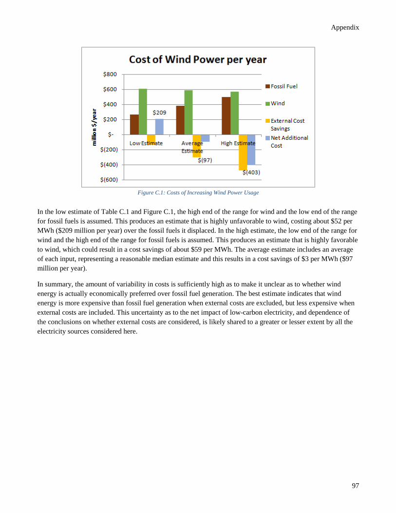
Appendix

97

Figure C.1: Costs of Increasing Wind Power Usage

In the low estimate of Table C.1 and Figure C.1, the high end of the range for wind and the low end of the range for fossil fuels is assumed. This produces an estimate that is highly unfavorable to wind, costing about $52 per MWh ($209 million per year) over the fossil fuels it displaced. In the high estimate, the low end of the range for wind and the high end of the range for fossil fuels is assumed. This produces an estimate that is highly favorable to wind, which could result in a cost savings of about $59 per MWh. The average estimate includes an average of each input, representing a reasonable median estimate and this results in a cost savings of $3 per MWh ($97 million per year).

In summary, the amount of variability in costs is sufficiently high as to make it unclear as to whether wind energy is actually economically preferred over fossil fuel generation. The best estimate indicates that wind energy is more expensive than fossil fuel generation when external costs are excluded, but less expensive when external costs are included. This uncertainty as to the net impact of low-carbon electricity, and dependence of the conclusions on whether external costs are considered, is likely shared to a greater or lesser extent by all the electricity sources considered here.