ordered probit - purdue universityweb.ics.purdue.edu/~jltobias/674/oprobit.pdf · ordered probit...

Ordered Probit

Econ 674

Purdue University

March 9, 2009

Justin L. Tobias (Purdue) Ordered Probit March 9, 2009 1 / 25

In some cases, the variable to be modeled has a natural ordinalinterpretation.

Some examples include:

1 Education, measured categorically, (e.g. 1 =< HS, 2 = HS , 3 =Some college, etc.).

2 Income, also measured categorically.

3 Survey responses, coded as a degree of opinion (e.g. 1 = StronglyDisagree, 2= Disagree, 3 = Agree, 4 = Strongly Agree.

4 These are in contrast to other choices such as type of insurance orselected mode of transportation, for example, that are not ordered.

In this lecture we discuss ordinal choice models, and focus on theordered probit in particular.


The Ordered Probit Model

Suppose that the variable to be modeled, y takes on J different values,which are naturally ordered:

yi =

12...J

, i = 1, 2, . . . , n.

As with the probit model, we assume that the observed y is generated by alatent variable y∗, where

The link between the latent and observed data is given as follows:



The αj are called cutpoints or threshold parameters. They are estimatedby the data and help to match the probabilities associated with eachdiscrete outcome.

Without any additional structure, the model is not identified. In particular,there are too many cutpoints and some restrictions are required. The mostcommon way to achieve identification is to set:

and retain an intercept parameter in the model.

What happens, for example when J = 2 and these restrictions areimposed?



The likelihood for the ordered probit is simply the product of theprobabilities associated with each discrete outcome:

L(β, α) =n∏

i=1

Pr(yi = j |xi ),

whereα = [α3 α4 · · · αJ ].

The i th observation’s contribution to the likelihood is



Therefore,

L(β, α) =n∏

i=1

Φ(αyi +1 − xiβ)− Φ(αyi − xiβ)

and

For purposes of computing the MLE, it can be useful to define

Zij = I (yi = j).

Thus, we can write:

L(β, α) =n∑

i=1

J∑j=1

zij (log [Φ(αj+1 − xiβ)− Φ(αj − xiβ)]) .

(Some textbooks present the material this way, though we will not makeuse of this here).



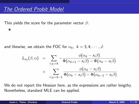
This yields the score for the parameter vector β:

and likewise, we obtain the FOC for αk , k = 3, 4, · · · , J:

Lαk(β, α) =

∑i :yi =k

− φ(αk − xiβ)

Φ(αk+1 − xiβ)− Φ(αk − xiβ)

+∑

i :yi =k−1

φ(αk − xiβ)

Φ(αk − xiβ)− Φ(αk−1 − xiβ)

We do not report the Hessian here, as the expressions are rather lengthy.Nonetheless, standard MLE can be applied.


Marginal Effects

To fix ideas, consider the case of an ordered probit model with J = 3, inwhich case we have:

From these, we obtain the category-specific marginal effects:


Marginal Effects

What do we learn from this simple model?

1 Like the probit, the marginal effects depend on x . We can evaluatethese at sample means, or take a sample average of the marginaleffects.

2 Unlike the probit, the signs of the “interior” marginal effects areunknown and not completely determined by the sign of βk .

3 We can, however, sign the effects of the lowest and highest categoriesbased on βk . The others, however, can not be known by the readersimply by looking at a table of point estimates.


Interpretation

Continue to consider the case with J = 3 and suppose there are nocovariates and only an intercept parameter is included.In this case we have

Pr(yi = 1) = 1− Φ(β)

Pr(yi = 2) = Φ(α− β)− [1− Φ(β)] = Φ(α− β)− Φ(−β)

Pr(yi = 3) = 1− Φ(α− β)

What do you think will happen in terms of the MLE’s?The likelihood is:

L(α, β) =∏

i :yi =1

[1− Φ(β)]∏

i :yi =2

[Φ(α− β)− Φ(−β)]∏

i :yi =3

[1− Φ(α− β)]

which reduces to


Interpretation

In the last slide, we have defined nj as the number of observations forwhich yi = j and also note that n1 + n2 + n3 = n.Thus we obtain the log-likelihood

L(α, β) = n1 log[1−Φ(β)]+n2 log[Φ(α−β)−Φ(−β)]+n3 log[1−Φ(α−β)].

The α FOC gives:

with P̂j denoting the fitted probability for category j .


Interpretation

Likewise, we get an FOC for β:

−n1φ(β̂)

1− Φ(β̂)+ n2

φ(β̂)− φ(α̂− β̂)

Φ(α̂− β̂)− Φ(−β̂)+ n3

φ(α̂− β̂)

1− Φ(α̂− β̂)= 0.

Grouping terms, and using our α FOC, the β FOC can be shown to imply:

n2

P̂2

=n1

P̂1

.


interpretation

Noting thatP̂1 + P̂2 + P̂3 = 1

andn1 + n2 + n3 = n,

these two FOC’s can be manipulated to yield:

That is, the parameters will be selected so that the fitted values of eachcategory exactly match the observed frequencies of outcomes in thatcategory. Note that this generalizes to any J and any link function!For β̂, for example, we obtain:

1− Φ(β̂) = n1/n

or

β̂ = Φ−1

(n − n1

n

).


−2.5 −2 −1.5 −1 −0.5 0 0.5 1 1.5 2 2.50

0.1

0.2

0.3

0.4

0.5

0.6

0.7

0.8

0.9

1

1 − Φ (β)

Φ (α − β)

Pr(y=1)

Pr(y=2)

Pr(y=3)


Ordered Probit and the EM Algorithm

Suppose that J = 3 and consider the following model:

y∗i = xiβ + εi , εi |xiiid∼ N (0, 1)

and

yi =

1 if y∗i ≤ 02 if 0 < y∗i ≤ α3 if y∗i > α.

Let



This reparameterization defines an equivalent model:

where

Note that, in this representation, there are no unknown cutpoints.



Step 1: E-StepNote that

and thus

L(δ, σ2; z∗) = constant − n

2log(σ2)− 1

2σ2(z∗ − X δ)′(z∗ − X δ).

The E-step is completed by taking expectations over z∗|θ = θt , y :

E [L(δ, σ2; z∗)] ≡ constant− n

2log(σ2)− 1

2σ2Ez∗|θ=θt ,y (z∗−X δ)′(z∗−X δ).



Step 2: M-Step:To implement the M− step, we must evaluate this expectation and thenmaximize over δ and σ2.

You will probably recognize the δ-part of this exercise. It will followsimilarly to the probit, where:

with


To evaluate this mean, suppose

and we seek

That is,



Applying this result, we can evaluate µ(δt , σ2t , y)

µ(δt , σ2t , yi ) =

xiδt − σ φ(xiδt/σt)Φ(−xiδt/σt) if yi = 1

xiδt + σ φ(xiδt/σt)−φ([1−xiδt ]/σt)Φ([1−xiδt ]/σt)−Φ(−xiδt/σt) if yi = 2

xiδt + σ φ([1−xiδt ]/σt)1−Φ([1−xiδt ]/σt) if yi = 3

Thus, the parameters δ are easily updated.



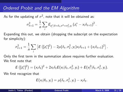
As for the updating of σ2, note that it will be obtained as:

σ2t+1 =

1

n

∑i

Ez∗i |δ=δt ,σ2=σ2t ,yi

(z∗i − xiδt+1)2 .

Expanding this out, we obtain (dropping the subscript on the expectationfor simplicity):

σ2t+1 =

1

n

∑i

[E([z∗i ]2

)− 2µ(δt , σ

2t , yi )xiδt+1 + (xiδt+1)2

].

Only the first term in the summation above requires further evaluation.We first note that

E([z∗i ]2

)= (xiδt)2 + 2xiδtE (vi |δt , σ2

t , yi ) + E (v 2i |δt , σ2

t , yi ).

We first recognize that

E (vi |θt , yi ) = µ(δt , σ2t , yi )− xiδt .



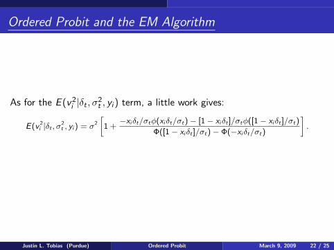
As for the E (v 2i |δt , σ2

t , yi ) term, a little work gives:

E(v 2i |δt , σ2

t , yi ) = σ2

[1 +−xiδt/σtφ(xiδt/σt)− [1− xiδt ]/σtφ([1− xiδt ]/σt)

Φ([1− xiδt ]/σt)− Φ(−xiδt/σt)

].



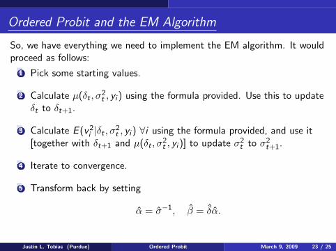
So, we have everything we need to implement the EM algorithm. It wouldproceed as follows:

1 Pick some starting values.

2 Calculate µ(δt , σ2t , yi ) using the formula provided. Use this to update

δt to δt+1.

3 Calculate E (v 2i |δt , σ2

t , yi ) ∀i using the formula provided, and use it[together with δt+1 and µ(δt , σ

2t , yi )] to update σ2

t to σ2t+1.

4 Iterate to convergence.

5 Transform back by setting

α̂ = σ̂−1, β̂ = δ̂α̂.



We use n = 139 law school applications from 1985.

The dependent variable is the rank of the law school with y = 1 if therank is less than or equal to 25, y = 2 if the rank is between 25 and 50and y = 3 if the rank exceeds 50.

The independent variables include the applicant’s LSAT score, GPA andstudent/faculty ratio (the latter is rather questionable).

In the following slides, we present the EM ordered probit estimates (whichmatched STATA’s EXACTLY and were obtained faster!) We report somestatistics evaluated at the sample mean of the x’s and also setting LSATand GPA to their maximum sample values.



β̂ = [49.1 − .24 − 2.73 − .01], α̂ = 1.00.

Category Fitted Probability Marginal Effectxbar xmax LSAT/xbar LSAT/ xmax GPA/ xbar

y = 1 .04 .99 .02 .003 .25y = 2 .20 .01 .05 -.003 .59y = 3 .76 .00 -.08 .000 -.85


ordered probit - purdue universityweb.ics.purdue.edu/~jltobias/674/oprobit.pdf · ordered probit...

Documents