outcome uncertainty and attendance demand in sport: the ... · probability model for match outcomes...
TRANSCRIPT

..........
.....
......
.....
.....
.....
......
.....
.....
.....
......
.....
.....
.....
......
.....
......
.....
.....
.
Outcome uncertainty and attendance demand in sport:the case of English soccer
Forrest, D., & Simmons, R. (2002)Journal of the Royal Statistical Society
Presenter: Sarah Kim2019.01.25

..........
.....
......
.....
.....
.....
......
.....
.....
.....
......
.....
.....
.....
......
.....
......
.....
.....
.
Introduction
▶ Uncertainty of outcome:A situation where a given contest within a league structure has a degree ofunpredictability about the result.
▶ Using betting odds by bookmakers, we set up a measure of uncertainty ofoutcome.
▶ Given suitable controls, we find that soccer match attendances are indeedmaximized where the uncertainty of outcome is greatest.

..........
.....
......
.....
.....
.....
......
.....
.....
.....
......
.....
.....
.....
......
.....
......
.....
.....
.
Data
1. Attendace data▶ We collected data for all matches played on Sat. between 1997.10 and
1998.05 and excluded the Augest and September period because weintended to use as regressors.
▶ We consider only the 872 matches played in divisions 1, 2 and 3 of theFootball League.
2. Betting data▶ Fixed odds betting: British bookmakers set the odds of scoccer bets several
days before a match and then these remain unaltered through the bettingperiod.
▶ For each match in our sample, we collected the odds for a home team win,draw and away team win.

..........
.....
......
.....
.....
.....
......
.....
.....
.....
......
.....
.....
.....
......
.....
......
.....
.....
.
Probability model for match outcomes
▶ First using an ordered probit model, we regress match outcomes (homewin, 0; draw, 1; away win, 2) on BOOKPROB(H) and DIFFATTEND:
▶ BOOKPROB(H):= podds(H)/∑
e∈{H, D, A} podds(e) for e ∈ {H, D, A},and podds is the probability odds (e.g. 3 : 1 becomes 0.25).
▶ DIFFATTEND:= (the mean home club home attendance for the previousseason)−(the mean away club home attendance for the previous season).
▶ We have a latent regression given by
y∗ = β1BOOKPROB(H) + β2DIFFATTEND + ϵ,
where y∗ is an unobserved latent variable, and ϵ is a normally distributederror term.

..........
.....
......
.....
.....
.....
......
.....
.....
.....
......
.....
.....
.....
......
.....
......
.....
.....
.
Probability model for match outcomes
▶ We observe▶ RESULT = 0 if y∗ ≤ 0,
▶ RESULT = 1 if 0 < y∗ ≤ µ,
▶ RESULT = 2 if µ ≤ y∗,
where µ is a threshold parameter to be estimated.▶ We have the following probabilities:
▶ Prob(RESULT = 0) = 1− Φ(β′x)▶ Prob(RESULT = 1) = Φ(µ− β′x)− Φ(−β′x)▶ Prob(RESULT = 2) = 1− Φ(µ− β′x),
where x = [BOOKPROB(H),DIFFATTEND].

..........
.....
......
.....
.....
.....
......
.....
.....
.....
......
.....
.....
.....
......
.....
......
.....
.....
.
Probability model for match outcomes
▶ The ordered probit regression equation was used to generate estimatedprobabilities of home wins and away wins.
▶ In the 872 matches, the predicted probability of an away win exceededthat of a home win in only 72 (8.2%) cases.
▶ Let “PROBRATIO” be the estimated ratio of the probability of a homewin to the probability of an away win.
▶ PROBRATIO is our measure of match uncertainty of outcome.

..........
.....
......
.....
.....
.....
......
.....
.....
.....
......
.....
.....
.....
......
.....
......
.....
.....
.
Attendance demand model
▶ Denote dependent variable LOGATTENDANCE by Ai where i is a hometeam identifier.
▶ Attendance demand model
Ai = α+ γ1PROBRATIOi + γ2PROBRATIO2i
+ γ3HOMEPOINTSi + γ4AWAYPOINTSi + γ5DISTi + γ6DIST2i
+ month dummies + error,
where DIST is the distance between grounds of competing teams.
▶ We include month dummay variables to capture the effects of weather,alternative seasonal attractions.

..........
.....
......
.....
.....
.....
......
.....
.....
.....
......
.....
.....
.....
......
.....
......
.....
.....
.
Results
..........
.....
......
.....
.....
.....
......
.....
.....
.....
......
.....
.....
.....
......
.....
......
.....
.....
.
Results
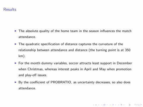
▶ The absolute quality of the home team in the season influences the matchattendance.
▶ The quadratic specification of distance captures the curvature of therelationship between attendance and distance (the turning point is at 350km).
▶ For the month dummy variables, soccer attracts least support in Decemberwhen Christmas, whereas interest peaks in April and May when promotionand play-off issues.
▶ By the coefficient of PROBRATIO, as uncertainty decreases, so also doesattendance.

..........
.....
......
.....
.....
.....
......
.....
.....
.....
......
.....
.....
.....
......
.....
......
.....
.....
.
On determining probability forecasts from betting odds
Štrumbelj, E. (2014)International journal of forecasting

..........
.....
......
.....
.....
.....
......
.....
.....
.....
......
.....
.....
.....
......
.....
......
.....
.....
.
Introduction
▶ There is substantial empirical evidence that betting odds are the mostaccurate publicly-available source of probability forecasts for spots.
▶ There are tow issues:1. Which method should be used to determine probability forecasts from raw
betting odds?2. Does it make a difference as to which bookmaker or betting exchange we
choose?

..........
.....
......
.....
.....
.....
......
.....
.....
.....
......
.....
.....
.....
......
.....
......
.....
.....
.
Determining outcome probabilities from betting odds1. Basic normalization
▶ Let o = (o1, . . . , on) be the quoted odds for a match with n ≥ 2 possibleoutcomes, and let oi > 1 for all i = 1, . . . , n.
▶ For each i, define a inverse odds πi =1oi
.
▶ Let β =∑n
i=1 πi be the booksum. Dividing by the booksum, pi =πiβ
canbe interpreted as outcome probabilites.
▶ We refer to this as basic normalization.

..........
.....
......
.....
.....
.....
......
.....
.....
.....
......
.....
.....
.....
......
.....
......
.....
.....
.
Determining outcome probabilities from betting oddsAssumptions of Shin’s model
▶ Shin’s model is based on the assumption that bookmakers odds whichmaximize their expected profit in the presence of uninforme bettors and aknown proportion of insider traders.
▶ The bookmaker and the uninformed bettors share the probabilistic beliefsp = (p1, . . . , pn), while the insiders know the actual outcome.
▶ W.L.O.G., assume that the total volume of bets is 1, of which 1− z comesfrom uninformed bettors and z from insiders.

..........
.....
......
.....
.....
.....
......
.....
.....
.....
......
.....
.....
.....
......
.....
......
.....
.....
.
Determining outcome probabilities from betting odds2. Shin’s model
▶ Conditional outcome i occuring, the expected volume bet on the ithoutcome is pi(1− z) + z.
▶ If the bookmaker quotes oi =1πi
for outcome i, the expected liability forthe outcome 1
πi(pi(1− z) + z).
▶ By assuming that the bookmaker has probabilistic beliefs p, thebookmaker’s unconditional expected liabilities is
∑ni=1
piπi(pi(1− z) + z),
and the total expected profit
T(π, p, z) = 1−n∑
i=1
piπi(pi(1− z) + z).
▶ The bookmaker sets π to maximize the expected profit, subject to0 ≤ πi ≤ 1.

..........
.....
......
.....
.....
.....
......
.....
.....
.....
......
.....
.....
.....
......
.....
......
.....
.....
.
Determining outcome probabilities from betting odds3. Regression analysis
▶ Use a statistical model to predict the outcome probabilities from odds.
▶ For sports with three outcomes (home, draw, away), we use an orderedlogistic regression model with (inverse) betting odds as input variables.
..........
.....
......
.....
.....
.....
......
.....
.....
.....
......
.....
.....
.....
......
.....
......
.....
.....
.
Comparison
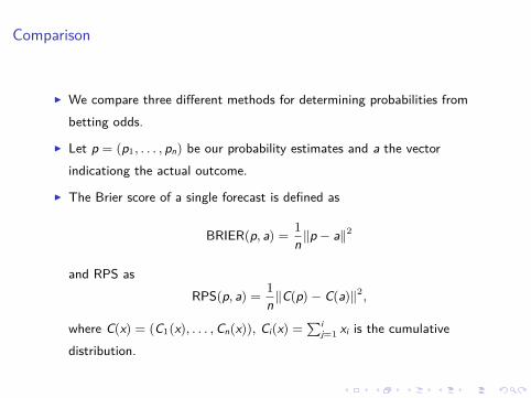
▶ We compare three different methods for determining probabilities frombetting odds.
▶ Let p = (p1, . . . , pn) be our probability estimates and a the vectorindicationg the actual outcome.
▶ The Brier score of a single forecast is defined as
BRIER(p, a) = 1
n∥p − a∥2
and RPS asRPS(p, a) = 1
n∥C(p)− C(a)∥2,
where C(x) = (C1(x), . . . ,Cn(x)), Ci(x) =∑i
j=1 xi is the cumulativedistribution.

..........
.....
......
.....
.....
.....
......
.....
.....
.....
......
.....
.....
.....
......
.....
......
.....
.....
.
Comparison
Figure : Comparison of three models using the Brier scores

..........
.....
......
.....
.....
.....
......
.....
.....
.....
......
.....
.....
.....
......
.....
......
.....
.....
.
Comparison
Figure : Comparison of bookmakers using the mean and median RPS scores