Organization and regulation of financial

systems

S8 DMC

Renaud Bourlès

Outline

B IntroductionILessons from the crisisIWhat is a bank and what do banks do?

BModels for banking regulationIDeposit insuranceILender of last resort: a simple model

BCapital reserves: the case of insuranceIOptimal choice of capital reserveIFailure risk and insurance demand

Grading

BThe evaluation of the course will be based onI an oral presentation

I by groups of 3 to 4 studentsI on a theme linked to real-world regulation

BThe list of themesI is available on Moodle

(the allocation taking place there)ITwo groups will work independently on each theme

Lessons from the (last) crisissee Tirole, in "Balancing the Banks", or

Beneplanc and Rochet: "Risk management in turbulent times"

BLast crisisI since 1970: 112 banking crises, affecting 93 countriesI 51 international crises (affecting several countries)

BFinancial madness?

IECON 101: all economic agents(incl. managers and employees in financial industries)

I react to the information and incentivesBBad incentives + bad information ⇒ Bad behavior

What happened?

BOrigin : home loans marketB then:

I sale of assets at fire-sale prices

I unprecedented aversion to risk

I freezing of interbank and bond marketB "government" reaction: bail-out ("renflouement") of some

of the largest banks and a major insurance company

An example: AIG

BBeginning of 2007I $ 1 trillion of assetsI $ 110 billion revenueI 74 million customers

B September 2008: emergency government assistanceI 2-year emergency loan of $ 85 billionI gvt hold 79.9% of shares

⇒ 50% of U.S. GDP has been guaranteed, lent or spentby the Fed, the US Treasury and other federal agencies

The role of subprime mortgages

BSubprime mortgages ("prêt hypothécaires"): loans w/ dif-ficulties in maintaining repayment scheduleI higher interest rateI less favorable terms (collateral)

to compensate for high risk

B losses on the US subprime market small relative to previ-ous figures ($1,000 billion, 4% of NYSE capitalization)

= detonator for a sequence of incentives and market failures(asym. info. betw/ contracting parties) exacerbated by badnews

Other issues

B bad regulation → incentives to take risk

B political resolution to favor real estate(to promote acquisition of homes by households)

Bmonetary policy: short term interest rate low

B excessive liquidityI international savings → US ⇒ excess liquidity⇒ securization ("titrisation") to answer the demand

Securization

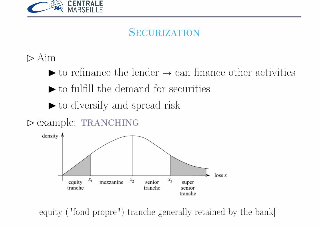
BAimI to refinance the lender → can finance other activitiesI to fulfill the demand for securitiesI to diversify and spread risk

B example: tranching

[equity ("fond propre") tranche generally retained by the bank]

Securization: CDO

BCollateralized Debt ObligationI the bank issues bonds against investmentI prioritized by different tranches

I ex: 3 loans of nominal 1, each w/ proba 10% of defaultand 0 recovery in case of default

IP(i defaults) =(in

)pi(1− p)n−i

P(1 d) = 24.3%, P(2 d) = 2.7%, P(3 d) = 0.1%

I equity tranche: loss up to 1mezzanine tranche: loss between x1 = 1 and x2 = 2

senior: losses above x2 = 2

Securization: CDS

BCredit Default SwapI contract between two partiesI the protection buyers pays a period premiumI to the protection seller who, in exchange,I commit to pay a fixed sum if a credit instrument

(a bond or a loan) default

B different for insuranceI the buyer doesn’t necessarily own the credit in-

strumentI the seller is not a regulated entity

Securization: Issues

B shift the responsibility away from the lender⇒ less incentive to control

B asymmetry of information

B laxity of credit-rating agencies

B excessive maturity transformation

The Northern Rock example

B strategy: invest in (apparently) safe tranches of Residen-tial Mortgage Backed Securities (RMBS)

B financed by short term deposit

B problem: rumors (risk on RMBS) ⇒ panic ⇒ bank run

⇒ nationalization: injection of £23 billion

B lack of liquidity also led to default of Lehman Brothers(biggest default in the US history: $ 613 bn of debt)

How to regulate?

BBasel accords: requirement regarding the minimal levelof capital or equity ("fonds propres")

BBasel I: requires 8% of bank credit risk

BProblemsIOther risks? Liquidity risks? Off balance-sheet?IRisk measure?I InformationI Incentives. Ex: managerial incentives (stock op-

tions). The CEO of Lehman Brothers earned $ 250million between 2004 and 2007

ISystemic institutions: Too Big To Fail

Basel II

B published in 2004, "implemented" in 2008

Pillar I Pillar II Pillar IIIMinimal Capital Supervisory DisclosureRequirement Review Process requirement

B Credit Risk B Regulatory framework B Disclosure onI Internal cap. adequacy capital, risk exposures,I Risk management risk assessment process

B Market Risk B Supervisory framework capital adequacyI Evaluation of internal

B Operational Risk systems B ComparabilityI Assessment of risk profile

BBasel III published in 2010, not yet fully implementedB tries to also account for liquidity risk

B and SIFIs (Systemically important financial institutions)

What is a bank and what do banks do? (1)see Freixas and Rochet: "Microeconomics of banking"

BBanking operations varied and complex

BBut a simple operational def (used by regulators) is"a bank is an institution whose current operations consist ingranting loans and receiving deposits from the public"Bcurrent important: most firms occasionally lend money

to customers or borrow from suppliers.BBoth loans and deposits important: combination of

lending and borrowing typical of commercial banks. Financea significant share of loans through deposits → fragility.

B public: not armed (6= professional investors) to assess safetyfinancial institutions. Public good (access to safe and effi-cient payment system) provided by private institutions

What is a bank and what do banks do? (2)

BProtection of depositors + safety and efficiency of paymentsystem → public intervention

BCrucial role in allocation of capitalI efficient life-cycle allocation of household consumptionI efficient allocation of capital to its most productive use

B before performed by banks alone; now fin. markets alsoB 4 functions performed by banks

IOffering liquidity and payment servicesITransforming assetsIManaging risksIProcessing information and monitoring borrowers

Liquidity and Payment Services

BWithout transaction costs (Arrow-Debreu): no need for money.B frictions → more efficient to exchange goods for money.B commodity money ("m. marchandise") → fiat money ("m.

fiduciaire"): medium of exchange, intrinsically useless,guaranteed by some institution

BRole of banksImoney change (exchange between different currencies

issued by distinct institutions) ⇒ dvlp of trade+management of deposits (less liquid, safer)I payment services: species inadequate for large or at

distance payments→ banks played an important part in clearing positions

Transforming Assets

Asset transformation can be seen from three viewpoints:

B convenience of denomination (size). Ex: small deposi-tors facing large investors willing to borrow indivisible amounts.

Bquality transformation: better risk-return characteristicsthan direct investments (diversified portfolio, better info)

Bmaturity transformation: transforms short maturities (de-posits) into long maturities (loans) → risk of illiquiditySolution: interbank lending and derivative financial in-struments (swaps, futures)

Managing risk

BCredit risk ⇒ use of collateral

BLiquidity risk ⇒ interest rate

BOff-Balance-sheet risk: competition ⇒ more sophisti-cated contractsI loan commitment, credit linesI guarantees and swaps (CDS)I hedging contracts ("opération de couverture")

B not real liability (or asset): conditional commitment

⇒ need of careful regulation

Monitoring and information processing

BProblems resulting from imperfect information on bor-rowers.

⇒ Banks invest in technologies that allow themI to screen loan applicants andI to monitor their projects

BLong-term relationships: mitigates moral hazard

A simple model with moral hazardBFirms seek to finance investment projects of a size 1BRisk-free rate of interest normalized to zero.BFirms have choice between

I a good technology: G with proba. ΠG (0 otherwise)I a bad technology: B with proba. ΠB (0 otherwise)

BOnly G proj. have positive net (expected) present value:ΠGG > 1 > ΠBB

but B > G, (which implies ΠG > ΠB)B Success verifiable, not choice of techno. (nor return)→ can promise to repay R (nominal debt) only if success+ no other source of cash → repayment zero if failsB value of R determines choice of technology

In the absence of monitoringB chooses G techno. iif gives higher expected profit:

ΠG(G−R) > ΠB(B −R)

B Since ΠG > ΠB this is equivalent toR < RC ≡ ΠGG−ΠBB

ΠG−ΠB

⇒Proba Π of repayment depends on R:

Π(R) =

{ΠG if R ≤ RCΠB if R > RC

BCompetitive equilibrium → Π(R).R = 1

B as ΠBR < 1 ∀R < B, only possible eq.: GBworks only if: ΠGRC ≥ 1, i.e. RC high enough↔ if moral hazard not too importantB otherwise: no trade (no credit market)

Including monitoring

B at cost C, banks can prevent from using bad techno⇒ new equilibrium interest rate: ΠGRm = 1 + C

B bank lending appear at equilibrium if (as Rm < G):I ΠGG > 1 + C ↔ monitoring cost lower than the NPVI ΠGRC < 1 ↔ direct lending (less expensive) not possible

B that is for intermediate values of ΠG:

ΠG ∈[

1 + C

G,

1

RC

]

Conclusion

BAssuming the monitoring cost C small enough so that1

RC>

1 + C

G

B 3 possible regimes of the credit market at equilibrium:

I if ΠG > 1RC

: firms issue direct debt at rate R1 = 1ΠG

I if ΠG ∈[

1+CG , 1

RC

]: borrow from banks at rate R2 = 1+C

ΠG

I if ΠG < 1+CG : credit market collapses (no trade eq.)

Possible extensions

BDynamic model (2 dates) with reputationI repayment at t = 1 → possibility of (cheaper) direct

loan at t = 2

IRt=1 < RC (reputation ↓ moral hazard); Rt=2U > RC

BUse of capital (choice between capital and debt)Iwell capitalized → direct loanI intermediate capitalization → bank loanI under-capitalized → no loan

→ substituability between capital and monitoring

Recall: why to regulate? (1)

B In general: Welfare theoremsBRegulation iif market failures:

externalities, asymmetric informationBBanks (or fin. intermediaries) solve some of these problemsBBUT create others:

I liquidity risk: assets illiquid, liabilities liquidAssets Liabilities

DepositsLoans

Capital (bonds)Reserves

Recall: why to regulate? (2)

B to protect clients (small depositors)I 6= other institutions: creditors = public→ no monitoring powerI creditor of other firms: BANKS (can monitor)

+conflict of interests btw/ manager and depositorsmanagers take too much risk (not their mean of payment)

+cost of failure: contagion + confidence on the sys-tem of payment

⇒Deposit Insurance + Lender of last resort +Capital ratio (+ Takeover ultimately)

Deposit InsuranceB to avoid bank panics and their social costsB governments have established deposit insurance schemes:

banks pay a premium to a deposit insurance fundB ex Federal Deposit Insurance Corporation in the U.S.

I created in 1933I in reaction to hundreds of failure in the 20s and 30s

Bmostly public schemesB pros

I systemic risk → private sector not "credible"I take-off decisions = public

B cons: lack of competitionI less incentive to extract info and price accurately

Deposit Insurance: a modelsee Freixas and Rochet: "Microeconomics of banking" (section 9.3)

B 2 dates: t = 0 and t = 1

B at t = 0 the bank:I issues equity E

I receives deposits DI loans LI pays deposit insurance premiums P

Assets LiabilitiesLoans L Deposits D

Insurance Premiums P Equity E

B normalize the risk-free rate to 0

B at t = 1 the bank is liquidatedB depositors compensated if bank’s assets insufficient

Assets LiabilitiesLoan repayments L1 Deposits DInsurance payments S Liquidation value V

B from t = 0: V , S and L1 are stochastic: V , S and L1

Bwith V = L1 −D + S

B insurance pays difference betw/ deposits (to "pay back")and loan repayments:

S = max(0, D − L1)

Bmoreover from t = 0: D = L + P − E

B therefore:V = E + (L1 − L) + [max(0, D − L1)− P ]

B shareholders’ value of the bank = its initial value + theincrease in the value of loans + net subsidy (<0 or >0)received from deposit insurance.

B if for example

L1 =

{X with prob. θ0 with prob. 1− θ

B the expected gain for the bank’s shareholders isE(Π) ≡ E

(V)− E

= (θX − L)︸ ︷︷ ︸net present value of loans

+ ((1− θ)D − P )︸ ︷︷ ︸net subsidy from insurance

E(Π) = (θX − L) + ((1− θ)D − P )

BProblem: create moral hazardI Suppose P fixed, andI banks choose characteristics (θ,X) of projectsIThen, within projects with same NPV: θX − L = cstI they choose those with lowest θ (i.e. highest risk)

BWhy?I P/D (premium rate) does not depend risk takenI as it was the case in the United States until 1991I then new system with risk-related premiums

Lender of Last Resort: a solution tocoordination failure

see Rochet and Vives, JEEA 2004

Motivation

BRole of government (or IMF):B lend to banks "illiquid but solvent"!B redundant w/ interbank market?

IYes! If the market works wellI i.e. without asymmetric informationI if it can recognize solvent banks

Lender of Last Resort: the model3 dates: τ = 0, 1, 2

B at τ = 0

I bank possesses own funds EI collects uninsured deposits D0 normalized to 1

give D > 1 when withdrawn (independ. of the date)I used to finance investment I in risky assets (loans)I the rest is held in cash reserves K

B under normal circumstances: I → R.I at τ = 2

deposits are reimbursed and shareholders get the differenceBBUT anticipated withdrawals (at τ = 1) can occur

depending on the signal received by depositors on R

B if proportion x > K: bank has to sell part of its assets

Assumptions

BWithdrawal decision taken by fund managersI in general they prefer not to do soIBUT are penalized by the investors if the bank fails

B consistent with observationsImajority of deposits held by collective investment fundsI remuneration of fund managers based on size not return

BModel: remun. based on whether take the "right decision"I if withdraw and not fail → −CI if withdraw and fail → B

B noting P the probability that bank fails: withdraw if

PB − (1− P )C > 0⇔ P > γ ≡ C

B + C

Signals and failure

At τ = 1

Bmanager i privately observes a signal si = R + εiwith εi i.i.d. and indep. from R

⇒ x% of the managers decide to withdraw

B if x > K/D the bank has to sell a volume y of its asset(repurchase agreement ∼ collateralized loan)I if y > I: the bank fails at τ = 1

I if R(I − y) < (1− x)D: the bank fails at τ = 2

Interbank market

B in case of liquidity shortage at τ = 1

I sell asset on repurchase agreement (or repo) marketI informationally efficient: resale price depend on R

IBUT cost (λ) of fire-sale (or liquidity premium)the bank only gets a fraction 1

1+λ of its asset value⇒ y / Ry

1+λ = [xD −K]+

⇔ y = (1 + λ)[xD−K]+

R

B λ is key to this analysisB reflects e.g. moral hazard: 2 reasons for selling asset

I needs liquidity or wants to get rid of bad loans (value 0)I 1

1+λ is then the proba of the former

Aim of the model

Bwant to show that interbank market does not suffice

B to prevent early closure of the bankB and so that we need a Lender of Last Resort

B if R small (close to insolvency) or λ large (liquidity shortage)B even with interbank market: early closure at τ = 1

BNow: early closure → physical liquidation of assets⇒ cost of liquidation (6= λ)Bmodel: if a bank closes at τ = 1, liquidation value νR withν << 1

1+λ

Bank runs and solvency (1)

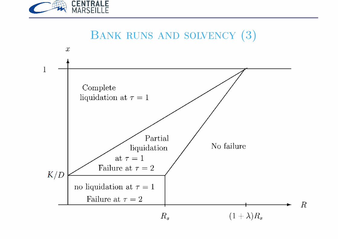
B if xD ≤ K: no sale of assets at τ = 1

⇒ failure at τ = 2 iif RI + K < D ⇔ R < D−KI ≡ RS

B if K < xD ≤ K + RI1+λ: partial sale of assets at τ = 1

⇒ failure at τ = 2 iifRI−(1+λ)(xD−K) < (1−x)D ⇔ R < RS+λ

xD −KI

≡ RF (x)

→Because of λ, solvent banks (R > RS) can failif R > (1 + λ)RS, never fails (even x = 1): super solvent

B if xD > K + RI1+λ: failure at τ = 1

⇔R < (1 + λ)xD−KI ≡ REC(x)

Bank runs and solvency (2)

B using the liquidity ratio: k = K/D, we have:

RS = 1−kI D, RF (x) = RS

(1 + λ

[x−k]+1−k

), REC(x) = RS (1 + λ)

[x−k]+1−k

B x ≤ 1⇒ RF (x) > REC(x)

B early closure implies failure(the converse is not true)

Bank runs and solvency (3)

Equilibrium of the Investors’ Game

BHow is x determined?Bwithout loss of generality, assume a threshold strategy

for all managersBwithdraw if signal s < t

B i.e. with proba: P(R + ε < t) = F (t−R)

where F is the c.d.f of εB this proba. also equals the proportion of withdrawals x(R, t)

Bmoreover, we assumed that managers withdraw ifB the probability of failure: P (s, t) > γ

⇔P(R < RF (x(R, t)) | s

)> γ ⇔ G(RF (t) | s) ≥ γ

where G(. | s) is the c.d.f. of R conditional on signal s

B now, as x(R, t) = F (t−R), RF is implicitly defined by:R = RS

(1 + λ

[F (t−R)−k

1−k

]+

)

Bwith t0/RF = RS, i.e. t0 = RS + F−1(k)

if t ≥ t0, "too many" failures → need for a LOLR

Strategic complementarity

B natural to assume G(r | s) decreasing in s:the higher s, the lower the proba that R < r

⇒ P (s, t) decreasing in s, increasing in t

(P (s, t): proba. of failure when signal s and threshold t)

⇒ P (s, t) > γ ⇔ s < s with s/P (s, t) = γ, i.e. s = S(t)

with S′(t) = −∂P/∂t∂P/∂s

≥ 0

⇒ a higher threshold t by others induces a manager to usea higher threshold also

Bayesian equilibrium (1)

Bwe look for a strategy such that the equilibriumis consistent with the beliefs

BManagers withdraw if P (s, t) > γ and withdraw if s < t

Bconsistent iif t∗/P (t∗, t∗) = γ

B then, as P (s, t) decreasing in s:I s < t∗ ⇒ P (s, t∗) > γ ⇒ withdrawI s > t∗ ⇒ P (s, t∗) < γ ⇒ not withdraw

Bayesian equilibrium (2)

BThe equilibrium (R∗F , t∗), where

I t∗ is the equilibrium withdrawal thresholdIR∗F is the equilibrium return threshold

is therefore determined by:{G(R∗F | t

∗) = γ

R∗F = RS

(1 + λ

[F (t∗−R∗F )−k

1−k

]+

)B 1st eq: if s = t∗, P(R < R∗F | s) = γ (def of t∗)B 2nd eq.: given t∗, R∗F is the return threshold, below which

failure occurs (def of R∗F )

Gaussian case

B to go further, we assumeBR ∼ N

(R, 1/α

)B ε ∼ N (0, 1/β) ⇒ F (x) = Φ(

√βx)

Bwe look for G(R | s) = G(R | R + ε). AsIR + ε ∼ N

(R, 1/α + 1/β

), and

I cov(R,R + ε) = Var(R) = 1/α

Bwe have R | R + ε ∼ N(αR+βsα+β , 1

α+β

)B that is G

(R∗F | t

∗) = Φ

(√α + βR∗F −

αR+βt∗√α+β

)

The equilibrium

BThe equilibrium is then characterizedB by a pair (t∗, R∗F ) such that Φ

(√α + βR∗F −

αR+βt∗√α+β

)= γ

R∗F = RS

(1 + λ

Φ(√β(t∗−R∗F ))−k

1−k

)B and we can prove (proof omitted) that

Proposition. When β (precision of private signal) largeenough relative to α (prior precision):

β ≥ 1

2π

(λαD

I

)2

≡ β0

unique t∗ such that P (t∗, t∗) = γ. The investor’s game thenhas a unique equilibrium: a strategy with threshold t∗.

Coordination failure

BFailure caused by illiquidity (coordination failure) if t∗ > t0

Bwith t∗ such that: Φ

(√α + βR∗F −

αR+βt∗√α+β

)= γ

B if t∗ ≤ t0: no coordination failure, i.e. R∗F = RS.In this case:

t∗ =1

β

((α + β)RS −

√α + βφ−1(γ)− αR

)B as t0 = RS + 1√

βφ−1(k)

B an equilibrium with t∗ ≤ t0 occurs iif:(α + β)RS ≤

√α + βφ−1(γ) + αR + βRS +

√βφ−1(k)

Liquidity ratio and coordination failure

BThat is iif:

k ≥ Φ

(α√β

(RS −R

)−√

1 +α

βΦ−1(γ)

)≡ k

Proposition. There is a critical liquidity ratio k of thebank such that, for k = K

D ≥ k only insolvent banksfail (there is no coordination failure).

B if k < k solvent but illiquid banks fail

Probability of failureB In this last case R∗F is defined by: Φ

(√α + βR∗F −

αR+βt∗√α+β

)= γ

R∗F = RS

(1 + λ

Φ(√β(t∗−R∗F ))−k

1−k

)⇔{−√α + βΦ−1(γ) + (α + β)R∗F − αR− βt

∗ = 0

t∗ = R∗F + 1√β

Φ−1(

1−kλRS

(R∗F −RS

)+ k)

⇔ α(R∗F −R

)− βΦ−1

(1−kλRS

(R∗F −RS

)+ k)−√α + βΦ−1(γ) = 0

BAs the l.h.s is decreasing in R∗F for β ≥ β0 we have

Proposition. R∗F – and therefore the proba of failure –is decreasing in the liquidity ratio k, the critical withdrawalprobability γ, and of the expected return R and increasingin the fire-sale premium λ and the face value of debt D.

How to avoid failure caused by illiquidity?

B theoretical possibility of a solvent bank being illiquid as aresult of coordination failure on the interbank market.

B 2 possibilities (for a central bank or a gvt) to eliminate that:I lower bond on the liquidity ratio k: kI decrease λ through:

liquidity injection (as for ex after Sept 11)discount-rate lending (ex. Fed ’08, low rate but stigma)

Discount-rate lending (1)

B fixing k ≥ k: costly in terms of "returns":I + K = 1 + E ⇒ high K means low investment

Bwhat to do if k < k?I assume that the central bank lends at rate r ∈ (0, λ)

without limit, BUT only to solvent banksICentral bank not supposed to subsidize: r > 0

I and assumed to perfectly observe R ← supervision

⇒Optimal strat. for a bank = lend exactly D(x− k)+

→ failure in τ = 2 iifRI < (1− x)D + (1 + r)(x− k)D

Discount-rate lending (2)

BThat is, as RS = D−KI =

D(1−k)I , iif

R < RS

(1 + r

[x− k]+1− k

)≡ R∗

(same as R∗F with r instead of λ)⇒ fully efficient (R∗ = RS) if r arbitrarily close to 0

+ central bank loses no money (loan repaid at τ = 2)as only lends to solvent banks (R > RS)

⇒ possible!

Possible extensions

B including moral hazardI investment in risky assets requires supervisionI supervision effort by bank manager e = {0, 1}, e = 1 costlyI e = 0⇒ R ∼ N

(R0,

1α

); e = 1⇒ R ∼ N

(R, 1

α

)with R > R0

IResult: the use of short-term debt is optimalallowing withdraw at τ = 1 discipline bank managers

B endogenizing k = K/D (reserves chosen by the bank)

Insurance, failure and reservessee Rees, Gravelle and Wambach, The Microeconomics of Insurance,

section 3.2

B insurance = promise (against a premium)to pay coverage in case of accident

B how to make sure this promise is kept?i.e. the insurance has enough reserve to pay coverage?

B has to ensure insurance doesn’t fail

B as banks: creditors of insurance companies are policy-holders

→cannot monitor their insurance company

⇒Existence of solvency rules and regulation authorities

The model

B an insurer offers a contract to n identical individualssame risk (distribution of claims identical), same preferences

B assume: independent risks (→ i.i.d.)not necessary to determine aggregate loss but simplifies

B Ci distrib of ind claims i.i.d.: mean µ and variance σ2

⇒ Cn =∑n

i=1 Ci distrib of aggregate claims, random var ofmean nµ

⇒ if premium sets to µ ("fair" premium) on each contractand insurance costs are zeroit will just break even ("rentable") in expected value:

E(Profit) = E(nµ− Cn

)= nµ−E

(Cn)

= 0

The need of reserves

BHoweverVar(Profit) = Var

(Cn)

= E((∑n

i=1 Ci − nµ)2)

= E[{∑n

i=1

(Ci − µ

)}2]

=∑n

i=1E[(Ci − µ

)2]

= nσ2

is positive and linearly increasing in n

B no convergence: ∀n, we can have Cn <> n.µ

⇒ to avoid insolvency

(when claims costs exceed funds available to meet them)insurance have to carry reserves.

Ruin probability (1)

B reasonable to assume maximum cover Cmax per contract⇒maximum possible aggregate claims cost: nCmax

⇒ if premium P and reserves Kmax = n(Cmax − P ):zero probability of insolvency

BHowever, in practice:I proba. total claims near nCmax extremely smallI raising capital of Kmax extremely costly

⇒ insurers choose a so-called ruin probability ρ

and given the distribution of Cn choose a level of reserves:K(ρ) = Cρ − nP with Cρ / P

(Cn > Cρ

)= ρ

Ruin probability (2)

B reserves / proba. ρ to be insolvent

B that is, when P = µ (fair premium)

How is ρ determined?

BTrade-off betweenI the costs associated with the risk of insolvency

depends on buyers’ perceptions of this riskI and the cost of holding reserves

B explored in more detail in the next sections

The implications of the Law of Large Numbers

B let C1, C2, ..., Cn the realizations of claims for n ind.(random sample from a distrib with mean µ and var σ2)

B let Cn = 1n

∑ni=1Ci be the sample mean

or the average loss per contract

BLaw of Large Numbers → ∀ε > 0, limn→∞

P(| Cn − µ |< ε

)= 1:

for sufficiently large n, virtually certain that the loss percontract equals µ, mean of individual loss distribution

BMoreover, Var(Cn)

= E((

1n

∑Ci − µ

)2)

= 1n

∑ni=1 σ

2 = σ2n

⇒ the variance of realized loss per contract goes to 0 as n→∞

Interpretation

B as the number of contracts sold becomes very large,B risk that realized loss per contract exceeds fair premium

becomes vanishingly small.

≈ economy of scaleI although variance of aggregate claims increases with n→ the reserves have to increase in absolute amount)

I the required reserve per contract tends toward zero

B required reserves increase less than proportionatelywith size of the insurer (number of contracts)

ExerciseConsider a portfolio of 400,000 identical contracts for whichB the number of accidents per contract (Ni) can be approxi-

mated by a P(0, 07)

B the expected value of claims per accident E(Cij) = 14500 e

Bwith a standard error σ(Cij) = 130000 e

BNi are assumed to be i.i.d ; Cij are assumed to be indep.from Ni, ∀j ; given Ni, Cij are assumed to be i.i.d ∀i, jICalculate the fair premium of a contractICalculate the standard error of the annual claims on a

contactICalculate the amount of reserves that makes the ruin

probability lower than 5% (assuming fair premia)

Optimal choice of reservessee Rees and Wambach, The Microeconomics of Insurance, section 3.5

B regulation: protect policyholders against risk of failureBreverse production cycle → risk of fraud:

once premiums paid insurer can run off

BBut large, well-established companiesI that wish to remain in business for the long termIwould not need detailed regulatory intervention,I to ensure they carry enough reserves to meet obligations

Bwant to model these effects

The key assumptions

1.Limited liability ("engagement limité")I a shareholder is liable for the debts of a company

only up to the value of his shareholding⇒ unregulated insurer may find optimal to put no reserves

and fail as soon as claims exceed collected premiums(more so if reserves are costly)

2. Increasing failure rated

dC

f (C)

1− F (C)> 0

met by virtually all insurance loss-claims distributions

The model (1)

B consider an insurance company in business for the long termB so taking decisions over an infinite time horizon

Bwith a sequence of discrete time periods (say years).

BAt the beginning of each year

B decide on a level of reserve capital KB given the distribution of claims C: F (C)

with (differentiable) density f (C), defined over [0, Cmax]

Bcostless reserves: owns (enough) capital but has to decidewhether to invest or to commit it in the insurance business

The model (2)

B premium income P exogenous (independent of K)buyers do not perceive relationship reserves and insolvencyand act as if no solvency risk

B P collected at the beginning of the periodand invested with K in riskless asset (return r > 1)

⇒At the end of the period assets: A = (P + K)r

I if A > C: remains in businessand receives continuation value V (expected present valueof returns from insurance business over all future periods)

I if A < C: defaultsA used to pay claims, loses Vlimited liability: doesn’t pay claims above A

Optimal reserves (1)

BC < Cmax⇒ can always choose to guarantee solvencyBQuestion: will insurers choose to stay solvent?

B it maximizes expected present value of future revenueB i.e. chooses at each period K ∈ [0, Kmax]

with Kmax = Cmaxr − P that

maxK

V0(K) =

∫ A

0

(V

r+ K + P − C

r

)f (C)dC −K

(if solvent at t = 1: r(K + P )− C + V )

B limited liability ⇒ upper limit Aif C > A: insolvent, pays out A, loses V ⇒ integrand = 0

Optimal reserves (2)

B infinite horizon: future identical at begin. of each period⇒ V = V0(K) and:

V0(K) =

[∫ A

0

(K + P − C

r

)f (C)dC −K

]/

[1− F (A)

r

]B put another way: at each period, if solvent,

i.e. with proba F (A) gets[∫ A

0

(K + P − C

r

)f (C)dC −K

]next period (discounted at rate 1/r):

V0(K) =

+∞∑t=0

(F (A)

r

)t[∫ A

0

(K + P − C

r

)f (C)dC −K

]

Corner solution

Proposition. If the claims distribution exhibits theincreasing failure rate property then the solution of theoptimization program of the insurer is a corner solution:

K = 0 or K = Kmax

Proof: There is no interior maximum:if ∃K∗ ∈ (0, Kmax)/V

′

0(K∗) = 0 then, under the assumption ofincreasing failure rate, V ′′0 (K∗) > 0

Proof (1): First order condition

V0(K) =

[∫ r(P+K)

0

(K + P − C

r

)f (C)dC −K

]/

[1− F (r(P+K))

r

]⇒ V

′

0(K) = 1(1−F (A)

r

)2(

(−1 + F (A) + 0).

(1− F (A)

r

)+ f (A)V0(K).

(1− F (A)

r

))(ddx

∫ u(x)

0f (x)dx =

∫ u(x)

0f ′(x)dx + f (u(x))u′(x)

)⇒ V

′

0(K∗) = 1

1−F (A)r

[V0(K∗)f (A)− (1− F (A))] = 0

where A = r(P + K)

Proof (2): Second order condition

⇒ V′′

0 (K) = 1

(1−Fr )

2

((V′

0(K)f + rV0(K)f ′ + rf).

(1− F (A)

r

)+ (V0(K)f − (1− F )) .f

)= 1

(1−Fr )

[V′

0(K)f + rV0(K)f ′ + rf + V′

0(K).f]

⇒ V′′

0 (K∗) = r(1−F

r )

[V0(K∗)f ′ + f

]Bwhat gives using the FOC V

′′

0 (K∗) = r(1−F

r )

[(1−F )f f ′ + f

]B now the assumption of increasing failure rate d

dCf (C)

1−F (C)>

0 gives (1− F )f ′ + f2 > 0

B 6 ∃K∗/V ′(K∗) = 0 and V′′(K∗) ≤ 0

Which corner?

⇒ no interior solutionB but continuous function on (0, Kmax) ⇒ ∃ maximum⇒ corner solution.BWhich corner? Compare V0(0) and V0(Kmax)

V0(0) =F (rP )

(rP − C0

)r − F (rP )

V0(Kmax) =rP − Cr − 1

with C ≡ E(C)

and C0 ≡ 1

F (rP )

∫ rP

0

CdF = E(C | C ≤ rP ) < C

Comparison

BAdvantage not to put any reserve:I decrease expected claim costs (C0 < C)I due to limited liability

BDisadvantageI risk 1− F (rP ) > 0 of going out of business

B In general, cannot say that a corner always better

Limitations of the model

B interest rate independent of the amount of capital raised

B no costs associated with raising capital

B exogeneity of premium: willingness to pay for insur-ance independent of insolvency riskI relaxed in the next model

Failure risk and insurance demand:see Rees, Gravelle and Wambach, Regulation of Insurance Markets,

GPRIT 1999

BAssume now that policyholders perfectly observe thereserves of their insurer

B and can infer from it its failure probability

BFirst: simplest case of just one insurance buyer withincome y (earned at end of period → "borrow" P )loss distribution F (.) on [0, Cu]

and utility function u(.) with u′> 0 and u

′′< 0

⇒ in the absence of insurance: expected utility:

u0 ≡∫ Cu

0

u(y − C)dF

Insurance demandBAssume insurer makes a "take-it-or-leave-it" offerB "full cover" (repayment=loss) at a premium P

BHowever, the buyer observes KB so the premium has to satisfy "participation constraint":∫ A

0

u(y − rP )dF +

∫ Cu

A

u(y − C − rP + A)dF ≥ u0

B note P0 the maximal premium the buyer accepts whenthe insurer has no capital: A = rP0:

P0 : F (rP0)u(y − rP0) +

∫ Cu

rP0

u(y − C)dF = u0

and Pu the maximal premium the buyer accepts whenthe insurer has maximum capital: A = Cu:Pu : u(y − rPu) = u0

Which corner?

Proposition. When the insurance buyer is fully in-formed about the insurer’s choice of capital; the in-surer’s expected value is larger at (Pu, Ku) than at(P0, K = 0).

Proof: we want to show that:1

r − 1

∫ Cu

0

(rPu − C)dF >1

r − F (rP0)

∫ rP0

0

(rP0 − C)dF

as r − 1 < r − F , a sufficient condition would be

rPu −∫ Cu

0

CdF > F (rP0)rP0 −∫ rP0

0

CdF

or rPu > F (rP0)rP0 +

∫ Cu

rP0

CdF

Proof: Jensen inequality (1)

B define P /u(y − rP ) = 11−F (rP0)

∫ Cu

rP0

u(y − C)dF

B Jensen: u(.) concave ⇒ ∀ random var. x : u(E(x)

)> E(u(x))

⇒ rP > 11−F (rP0)

∫ Cu

rP0

CdF ⇒ (1− F (rP0))rP >

∫ Cu

rP0

CdF

BMoreover:

(1− F (rP0))u(y − rP ) =

∫ Cu

rP0

u(y − C)dF

= u0 − F (rP0)u(y − rP0)

= u(y − Pu)− F (rP0)u(y − rP0)

⇒ u(y − rPu) = F (rP0)u(y − rP0) + (1− F (rP0))u(y − rP )

Proof: Jensen inequality (2)

BUsing again Jensen’s inequality, we have:rPu > F (rP0)rP0 + (1− F (rP0))rP

Bwhat implies using previous result that:

rPu > F (rP0)rP0 +

∫ Cu

rP0

CdF

Q.E.D

(a similar result can be proved for any K < Ku)

Intuition

BDue to risk aversion (u(.) concave)B policyholder always prepared to pay more than fair premiumB to insure against insurer’s insolvency

⇒ the insurer (risk-neutral) gains at selling this⇒ he must put up enough capital to remain solvent

(For now only shown in the simple case of only one buyer)

Generalization to N policyholders

B need more assumptionsI on individual riskI on how A is shared in case of failure

Bwe assumeI i.i.d risk of losing L(< y) with proba p: C ∼ L ∗ B(n, p)

I in case of failure by the insurer, each policyholder• receive indemnity in full w/ proba A/C• receive noting with proba (1− A/C)

Participation constraint

B a policyholder willing to pay P for full coverage if:

(1− p)u(y − rP ) + p

{(1− π)u(y − rP )

+ π[

(1− θ)u(y − rP ) + θu(y − rP − L)]}≥ u0

with π: proba insurer insolvent given he suffers the lossand θ: proba he receives nothing in this case

B that is, noting q ≡ pπθ

(1− q)u(y − rP ) + qu(y − rP − L) ≥ u0

Reserve and failure

B Suppose insurer chooses reserves to meet a given num-ber n < N of loses. Then:

q = p

N−1∑m=n−1

(N − 1

m

)pm(1− p)N−1−m

(1− n

m + 1

)B can then prove equivalent result to previous Proposition

Proposition. If buyers know the probability q thatthey will not be compensated, the insurer maximizes hisexpected value by choosing a capital Km so that thereis no default risk (q = 0).

Km =N(L−rPm)

r w/ Pm largest acceptable premium for q = 0

Proof (similar)

Bwe want to show that, ∀q > 01

r − 1N(rPm − pL) >

1

r − (1− d)N(rPq − (p− q)L)

w/ d: default proba; Pq: largest acceptable premium for qB as q > 0⇒ r − 1 < r − (1− d), sufficient to show that

rPm ≥ rPq + qL

B by definition:u(y − rPm) = (1− q)u(y − rPq) + qu(y − rPq − L) = u0

B and Jensen’s inequality gives:rPm > (1− q)rPq + q(rPq + L) = rPq + qL

Q.E.D

Intuition (similar)

B policyholders always willing to pay more than the fairpremium

B to insure against insurer’s insolvency,B the insurer finds it profitable to sell him thisB but requires to put enough capital to remain solvent

Conclusions

B if policyholders naively believe that the their insurer wouldremain solventImight be optimal for insurers not to hold reserves

and to bear failure risk

BBut if policyholders perfectly informed about insur-ers failure riskI always optimal for insurers to reduce this risk to zero

⇒Principe of regulation: provide policyholders w/ in-formation about insurers failure riskIdisclosure on capital, risk exposure,...+minimal capital requirement ≈ maximal failure proba

Limitations of the model

B interest rate independent of the amount of capital raised

B no costs associated with raising capital

B impossibility to recapitalize at the end of each periodafter claims realization, if A < C, insurer might want toraise some capital to remain solvent

Allowing for recapitalizationsee Bourlès and Henriet, 2009

BRecall: Why to regulate?I asymmetric information → solution = disclosureI conflict of interest betw/ shareholders & policyholders

B for the insurer to fail:I not only reserves has to be insufficientI but also has to be suboptimal to recapitalize

B Including shareholders in the model, new choices:I if solvent: take dividend or increase reserves (new shares)I if insolvent: failure or recapitalize (increase reserves)

⇒ information on reserve not sufficientB failure also depends on recap policy ⇒ credibility issue

Full commitment

B In such a model, the insurance company has to chooseI how much capital it holds (K)I a recapitalization policy:

the interval of claims that will be indemnified (I)I an issuance and dividend policy

Bmoreover assume that capital is costly:return on reserves lower than interest rate

BFrom previous analysis:I if insurer can commit ex-ante on a recap. policyI it commit never to defaultI costly capital → K = 0, I = [0,+∞)

No commitment

B If insurer cannot credibly commit on I, ex-post:I insurer optimally default if amount needed to continueI is larger than the present value of the insurance company

BWhen reserves are unobservable, we can show thatI insurer never holds reserves: K∗ = 0

I shareholders take dividends as soon as possible(never leave money in the insurance company)

I failure occurs optimally when claims exceed the value ofthe company

No commitment - observable reserves

BWhen reserves are observableI optimal to hold reserves: K∗ > 0

I as it increases the maximal acceptable premiumI failure occurs optimally when claims exceed the value of

the companyIBut: threshold higher than in previous case:

higher premium → higher value⇒ lower proba of failure

Implications for regulation

B information disclosure gets part of the way

Breserve requirement can also be useful:by ↑ the value of the company, it ↓ the probability of failure

BBut best regulation would beI to make credible the commitment to always recap.I for ex. by setting a guarantee fundI but... would introduce moral hazard for shareholders

(no incentives to hold reserves)

Insurance regulatory framework:Solvency I

B "Current" European regulation: Solvency II established in 1973, amended in 2002I solvency margin requirements (SMR)I financial guarantee in addition to provisionsI reserves > SMR = 4% of provisions + 3%� of capital

at riskBSimple and robust framework BUT

I no "true" measure of risk taken by the insurerI no qualitative requirement (quality of data)I no diversification effectI no role for information

Insurance regulatory framework:Solvency II

BNew European regulation: Solvency IIIReform adopted in 2009 by the European ParliamentI came into effect on 1 January 2016

(after having been scheduled for 01/01/13 and 01/01/14...)

BRelies as Basel accords on 3 pillars:IPillar I: Quantitative requirementsIPillar II: Qualitative requirementsIPillar III: disclosure and transparency requirements

Pillar I Pillar II Pillar IIIQuantitative Qualitative Disclosurerequirement requirement requirement

B Asset evaluation B Internal control B Requirementfor standardized

B Risk definition B Risk management information formarket authority

B Evaluations of B Reinforcement and regulators, investorsI technical provisions harmonization of and policyholdersI "target" capital (SCR) external controlI minimum capital (MCR) at EU level B transparency of

financial reporting

Two levels of capital requirement

B SCR (Solvency Capital Requirement)I capital required to ensure that insurance company ableI to absorb significant unexpected events

(bicentennial event)I and guarantee solvency in face of such eventsI If capital < SCR: insurance is required to ↑ capitalITargeted value of capital

BMCR (Minimal Capital Requirement)I level for which insurer’s activity pose anIunacceptable risk to policyholdersI If capital < MCR: license withdrawn

& liabilities transferred to another insurer

How is the SCR calculated?

BRisk measureIV@R: value at riskIPotential loss to be suffered on a portfolio over a given

period with a given probability α

I= quantile of loss-and-profit distribution X

(asset variation; in our model X = nP − C):P(V@R1−α < X

)= α

BCalibration of the SCRI SCR = Value-at-Risk at 99.5% over 1-yearI failure probability on 1 year < 0.5%I able to absorb bicentennial (adverse) event

Value at Risk at 99.5%

Is it a good measure of risk?