orientation robust transmit polarisation diversity … · chapter 1 introduction 1 1.1 ... 1.5...
TRANSCRIPT

Orientation Robust Transmit
Polarisation Diversity Techniques
Brian Yu-Chieh Huang
B. Eng (Hons)
A Thesis Submitted in Fulfilment
of the Requirements for the Degree of
Doctor of Philosophy
at the
Queensland University of Technology
Networks and Communications
Science and Engineering Faculty
March 2014


Keywords
Polarisation diversity, power correlation coefficient, cross polarisaion discrimina-
tion, branch power ratio, multi carrier code division multiple access, multiple
access interference, antenna orientation, circular polarisation, elliptical polarisa-
tion.


Abstract
Multipath fading adversely effects mobile communication because erratic varia-
tions in signal intensity across short distances degrades communication quality
and interferes with signal detection. Diversity techniques counteract fading by
combining multiple signals affected by independent channel distortions to min-
imise signal nulls. Effective diversity performance require these signals to exhibit
equal average power and have uncorrelated fading.
Polarisation diversity is a form of antenna diversity that captures signals re-
siding in orthogonal polarisations using polarisation sensitive antennas. These
antennas can be mounted in close proximity, allowing for spatially compact an-
tenna structures. This property makes polarisation diversity the only option for
spatially confined applications.
The major disadvantage of traditional polarisation diversity is that the av-
erage power between captured signals is severely imbalanced. This imbalance is
influenced by channel depolarisation and geometries of the transmitter and re-
ceiver antennas. Existing research using specific antenna geometries in the mobile
uplink fails to account for varible transmitter and receiver orientations which also
contributes to the average power imbalance.
The solution for power balanced polarisation diversity branches that also
negate orientation effects is the combined use of specialised antenna geometries
and channel specific elliptically polarised signals. This research allows polarisa-
tion diversity to counteract signal fading more effectively, and therefore guaran-
tees greater reliability in mobile communications.


Table of Contents
Abstract iii
Table of Contents v
List of Figures ix
List of Tables xiii
List of Acronyms and Abbreviations xv
List of Publications xvii
Statement of Original Authorship xix
Acknowledgements xxi
Chapter 1 Introduction 1
1.1 Signal fading . . . . . . . . . . . . . . . . . . . . . . . . . . . . . 2
1.1.1 Average path loss . . . . . . . . . . . . . . . . . . . . . . . 2
1.1.2 Shadow fading . . . . . . . . . . . . . . . . . . . . . . . . . 3
1.1.3 Multipath fading . . . . . . . . . . . . . . . . . . . . . . . 3
1.2 The conditions for micro diversity . . . . . . . . . . . . . . . . . . 5
1.2.1 Fading correlation . . . . . . . . . . . . . . . . . . . . . . . 6
1.2.2 Average branch powers . . . . . . . . . . . . . . . . . . . . 6
1.3 Modes of micro diversity . . . . . . . . . . . . . . . . . . . . . . . 8
1.3.1 Time diversity . . . . . . . . . . . . . . . . . . . . . . . . . 8
1.3.2 Frequency diversity . . . . . . . . . . . . . . . . . . . . . . 9
1.3.3 Antenna diversity . . . . . . . . . . . . . . . . . . . . . . . 11
1.4 Thesis objectives and contributions . . . . . . . . . . . . . . . . . 14

TABLE OF CONTENTS
1.5 Organisation of this thesis . . . . . . . . . . . . . . . . . . . . . . 16
Chapter 2 Principles of Polarisation Diversity 19
2.1 A brief history . . . . . . . . . . . . . . . . . . . . . . . . . . . . . 20
2.2 Branch power ratio and power imbalance . . . . . . . . . . . . . . 22
2.3 Fading correlation coefficient . . . . . . . . . . . . . . . . . . . . . 25
2.4 Measures of diversity performance . . . . . . . . . . . . . . . . . . 27
2.5 Comparing spatial and polarisation diversity . . . . . . . . . . . . 29
2.6 Addressing the power imbalance problem . . . . . . . . . . . . . . 31
2.7 Power imbalance and orientation sensitivity . . . . . . . . . . . . 33
Chapter 3 Acceptable Bounds for Diversity Parameters 37
3.1 The MC-CDMA scheme . . . . . . . . . . . . . . . . . . . . . . . 38
3.2 Synchronous MC-CDMA . . . . . . . . . . . . . . . . . . . . . . . 42
3.3 Asynchronous MC-CDMA . . . . . . . . . . . . . . . . . . . . . . 48
3.4 Asynchronous MC-CDMA with polarisation diversity . . . . . . . 51
3.5 Summary . . . . . . . . . . . . . . . . . . . . . . . . . . . . . . . 56
Chapter 4 Model of the Generalised Polarisation Diversity System 59
4.1 System model . . . . . . . . . . . . . . . . . . . . . . . . . . . . . 60
4.1.1 Transmitter component . . . . . . . . . . . . . . . . . . . . 60
4.1.2 Polarisation channel . . . . . . . . . . . . . . . . . . . . . 61
4.1.3 Polarisation diversity receiver . . . . . . . . . . . . . . . . 62
4.2 Diversity parameters . . . . . . . . . . . . . . . . . . . . . . . . . 63
4.2.1 Branch power ratio . . . . . . . . . . . . . . . . . . . . . . 63
4.2.2 Correlation coefficient . . . . . . . . . . . . . . . . . . . . 64
4.3 Simulation parameters and procedures . . . . . . . . . . . . . . . 65
4.4 Summary . . . . . . . . . . . . . . . . . . . . . . . . . . . . . . . 66
Chapter 5 Polarisation Diversity using Linear Polarisation 69
5.1 Traditional polarisation diversity . . . . . . . . . . . . . . . . . . 70
5.1.1 Transmitter orientation for power balanced diversity branches 72
5.1.2 Performance of traditional polarisation diversity . . . . . . 73
5.2 Symmetric polarisation diversity . . . . . . . . . . . . . . . . . . . 74
5.2.1 Modifying the receiver orientation for power balance . . . 75
5.2.2 Performance of the symmetric polarisation diversity . . . . 76
5.3 Summary . . . . . . . . . . . . . . . . . . . . . . . . . . . . . . . 79
vi

Table of Contents
Chapter 6 Reducing Excess Correlation With Circular Polarisa-
tion 83
6.1 System model and diversity parameters . . . . . . . . . . . . . . . 84
6.1.1 Mobile uplink . . . . . . . . . . . . . . . . . . . . . . . . . 84
6.1.2 Mobile downlink . . . . . . . . . . . . . . . . . . . . . . . 86
6.2 Results . . . . . . . . . . . . . . . . . . . . . . . . . . . . . . . . . 88
6.2.1 Mobile uplink . . . . . . . . . . . . . . . . . . . . . . . . . 88
6.2.2 Mobile downlink . . . . . . . . . . . . . . . . . . . . . . . 89
6.3 Summary . . . . . . . . . . . . . . . . . . . . . . . . . . . . . . . 91
Chapter 7 Adaptive Elliptical Polarisation for Polarisation Diver-
sity 95
7.1 Downlink . . . . . . . . . . . . . . . . . . . . . . . . . . . . . . . 96
7.1.1 System model . . . . . . . . . . . . . . . . . . . . . . . . . 96
7.1.2 Optimising diversity parameters . . . . . . . . . . . . . . . 97
7.1.3 Downlink results . . . . . . . . . . . . . . . . . . . . . . . 100
7.2 Uplink . . . . . . . . . . . . . . . . . . . . . . . . . . . . . . . . . 107
7.2.1 System model . . . . . . . . . . . . . . . . . . . . . . . . . 107
7.2.2 Optimum parameters . . . . . . . . . . . . . . . . . . . . . 108
7.2.3 Uplink results . . . . . . . . . . . . . . . . . . . . . . . . . 111
7.3 Summary . . . . . . . . . . . . . . . . . . . . . . . . . . . . . . . 113
Chapter 8 Conclusion and future research 117
8.0.1 Future research . . . . . . . . . . . . . . . . . . . . . . . . 120
Appendix A Power Correlation Coefficient for the Generalised Po-
larisation Diversity Model 123
A.1 Moments E [R21] and E [R2
2] . . . . . . . . . . . . . . . . . . . . . 124
A.1.1 Moments E [R2x] and E
[R2
y
]. . . . . . . . . . . . . . . . . 125
A.1.2 Moment E[RxR
∗y +R∗
xRy
]. . . . . . . . . . . . . . . . . . 126
A.2 Joint Moment E [R21R
22] . . . . . . . . . . . . . . . . . . . . . . . . 127
A.2.1 Moment E [R4x] . . . . . . . . . . . . . . . . . . . . . . . . 128
A.2.2 Moment E[R4
y
]. . . . . . . . . . . . . . . . . . . . . . . . 129
A.2.3 Moment E[R2
xR2y
]. . . . . . . . . . . . . . . . . . . . . . 132
A.2.4 Moment E[R2
x
(RxR
∗y +R∗
xRy
)]. . . . . . . . . . . . . . . 132
A.2.5 Moment E[R2
y
(RxR
∗y +R∗
xRy
)]. . . . . . . . . . . . . . . 133
vii

TABLE OF CONTENTS
A.2.6 Moment E[(RxR
∗y +R∗
xRy
)2]. . . . . . . . . . . . . . . . 133
A.3 Simplification of E [R1R2]− E [R1]E [R2] . . . . . . . . . . . . . . 134
A.4 Moment E [R41] . . . . . . . . . . . . . . . . . . . . . . . . . . . . 135
A.5 Moment E [R42] . . . . . . . . . . . . . . . . . . . . . . . . . . . . 136
A.6 Simplification of E [R41]− E2 [R2
1] . . . . . . . . . . . . . . . . . . 136
A.7 Simplification of E [R42]− E2 [R2
2] . . . . . . . . . . . . . . . . . . 137
A.8 Generalised Correlation Coefficient Expression . . . . . . . . . . . 137
References 139
viii

List of Figures
1.1 Envelope of a 1.2 GHz signal subject to multipath fading. . . . . . . 4
1.2 Two signal envelopes with uncorrelated fading. . . . . . . . . . . . . 7
1.3 Two signal envelopes with correlated fading. . . . . . . . . . . . . . . 8
1.4 Diversity performance of independent and correlated fading. . . . . . 9
1.5 Diversity performance of average power balanced and imbalanced cases. 10
2.1 Probability distribution of a signal with Rayleigh fading. . . . . . . . 29
2.2 Diversity gain of a theoretical two branch selection combiner . . . . . 30
2.3 Comparison of performance between diversity schemes. . . . . . . . . 31
3.1 Overlapping OFDM frequency subcarriers. . . . . . . . . . . . . . . . 40
3.2 The synchronous MC-CDMA . . . . . . . . . . . . . . . . . . . . . . 43
3.3 Comparison of the BER between synchronous MC-CDMA systems
using equal gains and MAI cancellation gains . . . . . . . . . . . . . 47
3.4 The asynchronous MC-CDMA. . . . . . . . . . . . . . . . . . . . . . 48
3.5 BER performance of the asynchronous MC-CDMA. . . . . . . . . . . 51
3.6 Asynchronous MC-CDMA with polarisation diversity. . . . . . . . . . 52
3.7 BER performance of asynchronous MC-CDMA with polarisation di-
versity, under different levels of branch power imbalance. . . . . . . . 56
4.1 Generalised model of the transmitter component. . . . . . . . . . . . 60
4.2 Generalised model of the polarisation diversity receiver. . . . . . . . . 61
4.3 Generalised model of the polarisation diversity receiver. . . . . . . . . 62
5.1 The traditional polarisation diversity in the mobile uplink. . . . . . . 70
5.2 BPR simulation for the traditional polarisation diversity . . . . . . . 73
5.3 Correlation coefficient simulation for the traditional polarisation di-
versity . . . . . . . . . . . . . . . . . . . . . . . . . . . . . . . . . . . 74

LIST OF FIGURES
5.4 BPR simulation as a function of the receiver orientation ψ in an urban
environment. . . . . . . . . . . . . . . . . . . . . . . . . . . . . . . . 77
5.5 Correlation coefficient as a function of the receiver orientation ψ in
uncorrelated channels. . . . . . . . . . . . . . . . . . . . . . . . . . . 78
5.6 Correlation coefficient as a function of the receiver orientation ψ in
correlated channels. . . . . . . . . . . . . . . . . . . . . . . . . . . . . 78
6.1 Polarisation diversity using circular polarisation with variable trans-
mitter orientation in the mobile uplink. . . . . . . . . . . . . . . . . . 85
6.2 Polarisation diversity using circular polarisation with variable receiver
orientation in the mobile downlink. . . . . . . . . . . . . . . . . . . . 86
6.3 BPR simulation for the mobile uplink with circular polarisation . . . 89
6.4 Correlation coefficient simulation for the mobile uplink with circular
polarisation . . . . . . . . . . . . . . . . . . . . . . . . . . . . . . . . 90
6.5 BPR simulation for the mobile downlink with circular polarisation . . 91
6.6 Simulation of the correlation coefficient in the uncorrelated downlink.
Circular polarisation was transmitted. . . . . . . . . . . . . . . . . . 92
6.7 Simulation of the correlation coefficient in the correlated downlink.
Circular polarisation was transmitted. . . . . . . . . . . . . . . . . . 92
7.1 Downlink polarisation diversity with elliptical polarisation. . . . . . . 96
7.2 BPR of the linear, circular and elliptical polarisations in the urban
downlink. . . . . . . . . . . . . . . . . . . . . . . . . . . . . . . . . . 101
7.4 BPR of the linear, circular and elliptical polarisations in the rural
downlink . . . . . . . . . . . . . . . . . . . . . . . . . . . . . . . . . . 102
7.3 BPR of the linear, circular and elliptical polarisations in the suburban
downlink . . . . . . . . . . . . . . . . . . . . . . . . . . . . . . . . . . 102
7.5 Simulation of the correlation coefficient in an uncorrelated urban down-
link. . . . . . . . . . . . . . . . . . . . . . . . . . . . . . . . . . . . . 103
7.6 Simulation of the correlation coefficient in an uncorrelated suburban
downlink. . . . . . . . . . . . . . . . . . . . . . . . . . . . . . . . . . 104
7.7 Simulation of the correlation coefficient in an uncorrelated rural down-
link. . . . . . . . . . . . . . . . . . . . . . . . . . . . . . . . . . . . . 104
7.8 Simulation of the correlation coefficient in a correlated urban downlink.105
7.9 Simulation of the correlation coefficient in a correlated suburban down-
link. . . . . . . . . . . . . . . . . . . . . . . . . . . . . . . . . . . . . 106
x

List of Figures
7.10 Simulation of the correlation coefficient in a correlated rural downlink. 106
7.11 Uplink polarisation diversity with elliptical polarisation. . . . . . . . 107
7.12 Uplink simulation of the XPD as a function of the transmitter orien-
tation in an urban environment. . . . . . . . . . . . . . . . . . . . . . 112
7.13 Uplink simulation of the correlation coefficient as a function of the
transmitter orientation in an uncorrelated urban environment. . . . . 113
7.14 Uplink simulation of the correlation coefficient as a function of the
transmitter orientation in a correlated urban environment. . . . . . . 114
xi


List of Tables
4.1 Polarisation channel relative power ratios. . . . . . . . . . . . . . . . 66
5.1 Transmitter orientations for power balanced BPR. . . . . . . . . . . . 72
6.1 XPD obtained in each environment under circular polarisation . . . . 86
7.1 Operating parameters of elliptical polarisation . . . . . . . . . . . . . 101
7.2 Operating parameters for a mobile transmitter in an urban environ-
ment orientated at angles 20◦, 40◦ and 60◦. . . . . . . . . . . . . . . . 111


LIST OF ACRONYMS AND ABBREVIATIONS
List of Acronyms and
Abbreviations
4G The fourth generation of mobile communication systems
AWGN Additive white Gaussian noise
BER Bit error rate
bps Bits per second
BPSK Binary phase shift keying
BPR Branch power ratio
CDMA Code division multiple access
DS-CDMA Direct-sequence CDMA
EGC Equal gain combining
FFT Fast Fourier transform
Hpol Horizontal polarisation
HSPA+ Evolved high speed packet access
ICI Inter-channel interference
i.i.d. Independent and identically distributed
ISI Inter-symbol interference
LOS Line of sight
LTE Long term evolution
MAI Multiple access interference
MC-CDMA Multicarrier CDMA
NLOS No line-of-sight
OFDM Orthogonal frequency division multiplexing
PDF Probability density function
RMS Root mean square
RSSI Received signal strength indicator
SNR Signal-to-noise ratio
Vpol Vertical polarisation
XPD Cross polarisation discriminationxvi

List of Publications
Conference papers
• X. Li, Y.C. Huang and B. Senadji, “MAI Analysis of an Asynchronous
MC-CDMA System With Polarization Diversity”, The 1st International
Conference on Signal Processing and Communication Systems (ICSPCS
2007), Gold Coast, 2007.
• Y.C. Huang and B. Senadji, “Orientation Invariant Diversity Gain Using
Transmit Polarization Diversity”, The 2nd International Conference on Sig-
nal Processing and Communication Systems (ICSPCS 2008), Gold Coast
2008.
• Y.C. Huang and B. Senadji, “Orientation Adaptive Transmit Polarization
Diversity for Branch Power Equalization”, The 5th International Wire-
less Communications and Mobile Computing Conference (IWCMC 2009),
Leipzig, 2009.
• Y.C. Huang and B. Senadji, “A Simple Orientation Robust Transmit Po-
larization Signalling Scheme”, The 10th International Conference on Infor-
mation Sciences, Signal Processing and their Applications (ISSPA 2010),
Kuala Lumpur, 2010.
Papers submitted to journals
• Y.C. Huang, B. Senadji, J. Cotzee, D. Jayalath “Mobile Orientation Invari-
ant Power Balanced Polarization Diversity”, Electronics Letters, [Submit-
ted].


Statement of Original Authorship
The work contained in this thesis has not been previously submitted to meet
requirements for an award at this or any other higher education institution. To
the best of my knowledge and belief, the thesis contains no material previously
published or written by another person except where due reference is made.
Signature:
Date: 25 March, 2014
QUT Verified Signature


Acknowledgements
I would like to thank my supervisors Associate Professor Bouchra Senadji, Dr.
Dhammika Jayalath, and Dr. Tee Tang for their continuous support throughout
my candidature. I would especially like to thank Bouchra and Dhammika for
helping me overcome the technical challenges throughout my candidature.
I would also like to thank Karyn Gonano for her encouragement and friendship
during the last four months of the candidature.
I would also like to extend my gratitude to my friends in the lab, Xuan (Leo)
Li, Daniel Chen, David Wang, and Kevin Chang. It has been an absolute pleasure
working with you all.
Last but not least, I would like to thank my family and all of my friends for
their kind support throughout my candidature.


Chapter 1
Introduction
The challenge to provide undistorted, reliable and seamless communications whilst
on the move is a complex problem that continues to confront mobile communi-
cations engineers. The hostile and highly lossy nature of the mobile channel is
often regarded as the main reason for the difficulty of the task.
Signals in mobile communications are relayed between the transmitter and
receiver through the broadcast of radio waves into a shared wireless medium.
Signal coverage is established as the radio wave propagates throughout the cel-
lular region. However, there are no dedicated physical paths through which the
transmitted signals are guided, causing the majority of the transmit power to be
lost. Only a fraction of this power is ever recovered by the receiver.
Complications arising from the lossy nature of the mobile channel are fur-
ther exacerbated by the elevated levels of signal interference, imposing signal
distortions and disrupting the detection process. Interference is caused by the
emission of electromagnetic radiation from spurious currents which induce alter-
ations to the original signal. Examples include microwave background radiation,
co-channel interference, adjacent channel interference, inter-symbol interference,
inter-modulation interference, multi-user interference and hostile radio jamming
interference [86].
The already difficult task of establishing reliable communications in the mobile
channel is further worsened when signal fading, a consequence of the way signals
propagate in the mobile channel, impose further deteriorations on the transmitted
signal.

CHAPTER 1. Introduction
1.1 Signal fading
Signal fading is the loss of signal power due to the nature of signal propagation
within the mobile environment. Fading is generally characterised to exhibit both
large scale and small scale phenomena. Their classification depends on the dis-
tances considered across the duration of observation [43]. This allows for the
description of separate mechanisms which contribute to signal fading. The large
scale fading effects are characterised by path loss and shadow fading, while the
small scale fading is described by the multipath fading model.
1.1.1 Average path loss
The average path loss is a large scale fading effect that is observed when the
distances considered are in the order of several kilometres. This kind of fading is
primarily attributed to the loss of power density as propagating radio wavefronts
expand in space [56,93].
Theoretical and experimentally based path loss models in the literature agree
upon the logarithmic attenuation of signal power as a function of the distance
separating the transmitter and the receiver [29, 38, 100]. A popular model of the
log-distance path loss is based upon the Frii’s transmission formula
L (d) = L (d0) + 10n log10
(d
d0
), (1.1)
where L (d) is the average path loss in decibels (dB), d is the distance between the
transmitter and the receiver, and L (d0) is the reference path loss at a distance
d0 from the transmitter [79]. The path loss exponent n describes the rate at
which the average power density is lost as a function of distance. For free space
propagation, n is equal to 2, and the signal intensity is seen to be inversely
proportional to the square of the distance [82]. However, these values have been
reported to vary from 1.8 to 6, depending on the propagation environment [3,12,
29,77,79,93].
Accurate knowledge of the average path loss is important since it determines
the effective range of base stations and predicts the boundaries of cellular regions.
The strategic placement of base stations remains the most effective way to ensure
a reliable cellular coverage [40].
2

1.1 Signal fading
1.1.2 Shadow fading
Shadow fading is another large scale fading effect. This kind of fading is seen when
distances considered are in the order of several hundred meters. Shadow fading
describes the loss of power density as the transmitted signals engage with large
terrestrial obstacles over irregular terrain [72]. Major features of the environment
such as hills, and water surfaces can become refracting edges or reflecting sur-
faces that causes the average signal intensity to fluctuate randomly about a mean
intensity level previously predicted through the average path loss [79]. Though
shadow fading is predominantly influenced by major geographical features, ob-
jects along the path of propagation with the physical dimensions comparable to
the transmitted signal wavelength has the potential to influence the severity of
shadow fading [56].
Experimental measurements taken in the field demonstrate that amplitude
fluctuations are log-Normally distributed about a mean value predicted by the
average path loss [8,20,93]. The shadow fading component is incorporated math-
ematically into the average power loss with the addition of the shadow fading
component Xσ,
L (d) = L (d0) + 10n log10
(d
d0
)+Xσ , (1.2)
where Xσ is expressed in dB, and is modelled as a zero mean Gaussian random
variable, with a standard deviation σ which is also expressed in dB. Typical
values of σ can range from 6 dB to 8 dB and depends on the location [93]. An
effective way to counteract shadow fading is to assign multiple base stations to
simultaneously service a given cellular region [49].
1.1.3 Multipath fading
Small scale fading is observed when distances over a few tens of wavelengths are
considered. Small scale fading is sometimes also called multipath fading, as the
observed amplitude fluctuations are direct consequences of the constructive and
destructive interference caused by the multipath nature of signal propagation [39].
Multipath propagation occurs when radio signals broadcast by the transmit-
ter diverge and propagate over a number of independent routes before arriving
at the receiver. Signals in each route traverse different distances and converge on
3

CHAPTER 1. Introduction
0 50 100 150 200−50
−40
−30
−20
−10
0
10
Time (ms)
Sig
nal I
nten
sity
(dB
abo
ut R
MS
)
Figure 1.1: Envelope of a 1.2 GHz signal subject to multipath fading.
the receiver with different time delays and phase offsets. These wavefronts su-
perimpose upon arrival at the receiver and produce a standing wave environment
that exhibits peaks and nulls in the signal intensity [69]. Extreme variations in
the instantaneous power of the received signal occur across very short distances.
Fig. 1.1 illustrates the simulated envelope of a 1.2 GHz signal captured by a
mobile terminal travelling at 100 km/hr within a multipath fading environment.
Constructive interference may yield temporary peaks in the signal intensity, but
destructive interference can reduce intensity levels to 45 dB below the mean. Sig-
nal fades occur frequently, with successive instances appearing quasi periodically
at intervals of every half wavelength [79]. The rate at which signal nulls occur for
a mobile terminal travelling at this speed is in the order of a few hundred cycles
per second.
What can be inferred from such an observation is that the occurrence of
the deep fades will be at least an order of magnitude less frequent for mobiles
travelling at slower speeds. However, this does not mean that the degree of the
fades will have become any less severe. A reduction of the fading rate consequently
increases the duration of deep fades. Furthermore, if the mobile unit was to
4
1.2 The conditions for micro diversity
become stationary, there is always the possibility that it would land within one
of these deep fades [42], ultimately terminating any means of communications.
Given both the severity and frequency of the amplitude fluctuations, reliable
communications on the move becomes a formidable task. Preserving the link
quality is especially problematic since noise levels do not reduce following sudden
fades in signal strength.
1.2 The conditions for micro diversity
While the strategic placement of base stations to create overlapping cell tessel-
lations for better signal coverage can be used to negate large scale fading, small
scale fading can not be addressed in this manner. This is because small scale
fading is not the result of the dispersive loss of power, but rather the direct sig-
nal cancellation from the superposition of incoming signal wavefronts. Multipath
propagation still gives rise to the problem of small scale fading, irrespective of
the number of additional base stations installed.
Micro diversity techniques can be used to alleviate the effects of small scale
fading by addressing the problem with the objective of minimising the occurrences
of destructive interference [43]. This can be achieved if multiple independently
distorted copies of the transmitted signal are obtained and appropriately com-
bined. The fundamental principle at work is that a simultaneous signal null
across all received copies is significantly less probable compared with any indi-
vidual copy [96]. For instance, if two independently received signals subject to
unique fading effects each have a 10% probability of being within a -10 dB fade,
the probability of such event occurring simultaneously reduces significantly to
1%.
The improvement in fading reduction with this example is only possible on
the condition that the separate diversity signals are available, exhibit statisti-
cally independent fading, and have equal average signal power [14]. If fading
characteristics are not independent, the fading is said to be correlated, and the
effectiveness of diversity reduces since simultaneous fades become more likely.
A balanced average signal power is also important, as it ensures that diversity
sources can contribute equally in reducing the probability of the fades.
5

CHAPTER 1. Introduction
1.2.1 Fading correlation
Fading correlation measures the similarity of distortions observed between two
diversity signals. The correlation coefficient quantifies this similarity with a score
between 1 and -1 [74]. When the correlation coefficient equals 1, the fading is
said to be completely correlated, and exhibits no differences between the received
signals. On the other extreme, when the correlation coefficient is -1, the signal
fades are said to be anti-correlated. Theoretically, an anti-correlated pair of
equal power diversity signals with a selection combiner would negate the problem
of fading completely, since as one copy fades, the alternative copy peaks [90,96].
Although negative correlation coefficients have been observed in the literature
[15,27,59,97], these values have been close to 0. For Rayleigh channels, negative
correlation is impossible, and the case of statistically independent, or uncorrelated
fading with a coefficient of 0 is the best achievable outcome [97].
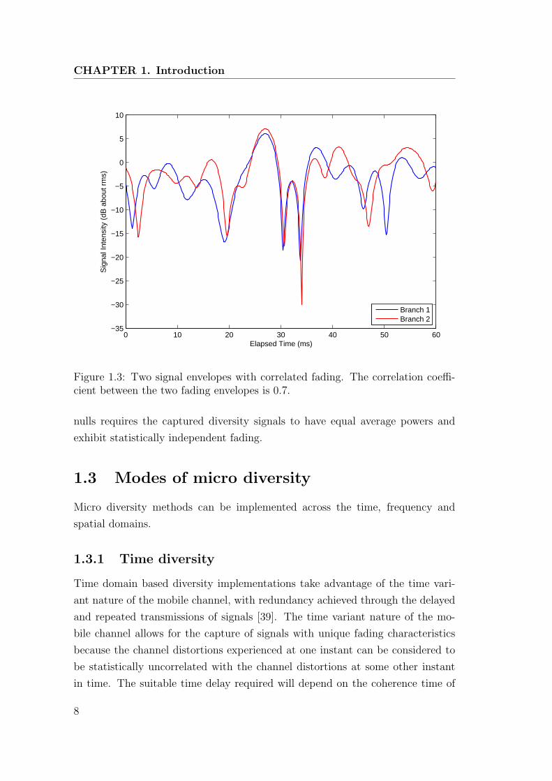
Fig. 1.2 and Fig. 1.3 are presented to illustrate the cases for correlated
and uncorrelated fading. The former features two envelopes with uncorrelated
fading, while the latter shows two envelopes subject to correlated fading with a
correlation coefficient of 0.7. Simultaneous fades are more likely to occur in the
latter case.
Diversity performance to alleviate the effects of fading decreases with increas-
ing fading correlation [54, 76]. Fig. 1.4 compares the probability distributions of
the signal envelope post recombination for the correlated and uncorrelated cases.
The correlation coefficient for the correlated case was set to 0.7, while the inde-
pendent case had its correlation coefficient set to 0. The single branch Rayleigh
distribution was included for reference. The figure shows that the probability
for the signal envelope to fall 15 dB below the mean is 0.1% in the uncorrelated
case, but increases to 0.3% for the correlated case. In the case of no diversity,
this probability is higher still, at 3%. The consensus in the literature for the
threshold of acceptable diversity is to maintain a fading correlation coefficient
below 0.7 [2, 31,43,47,48,94].
1.2.2 Average branch powers
A balanced average signal power ensures that uncorrelated diversity signals are
used to their full potential [35]. Diversity signals that exhibit equal average
power contribute equally in reducing the probability of fades. The comparison
6

1.2 The conditions for micro diversity
0 10 20 30 40 50 60−50
−40
−30
−20
−10
0
10
Elapsed Time (ms)
Sig
nal I
nten
sity
(dB
abo
ut r
ms)
Branch 1Branch 2
Figure 1.2: Two signal envelopes with uncorrelated fading.
of the average branch powers is quantified by the Branch Power Ratio (BPR),
and is defined as the quotient of the average power between two contributing
diversity signals, expressed in dB. The optimum case where branch powers are
equal corresponds to a BPR equal to 0 dB. Diversity performance is severely
compromised when the BPR is large because the weaker signal branch does not
contribute to reduce the probability of fades. In extreme cases, no diversity is
achieved [96].
The effects of power imbalance is illustrated in Fig. 1.5, which compares the
probability distribution functions of signal envelopes post diversity recombina-
tion. The standard two branch diversity with signal powers σ1 and σ2 has been
set to exhibit different levels of imbalance. As the imbalance increases, the prob-
ability distributions functions continues to push towards the left and approach
the scenario of the single branch Rayleigh envelope with no diversity benefits.
There appears to be little consensus as to what the threshold for an acceptable
BPR should be, with authors reporting acceptable diversity improvements despite
BPR values that are as high as 6 dB and 10 dB [24].
Optimum diversity action to most effectively minimise the occurrence of signal
7
CHAPTER 1. Introduction
0 10 20 30 40 50 60−35
−30
−25
−20
−15
−10
−5
0
5
10
Elapsed Time (ms)
Sig
nal I
nten
sity
(dB
abo
ut r
ms)
Branch 1Branch 2
Figure 1.3: Two signal envelopes with correlated fading. The correlation coeffi-cient between the two fading envelopes is 0.7.
nulls requires the captured diversity signals to have equal average powers and
exhibit statistically independent fading.
1.3 Modes of micro diversity
Micro diversity methods can be implemented across the time, frequency and
spatial domains.
1.3.1 Time diversity
Time domain based diversity implementations take advantage of the time vari-
ant nature of the mobile channel, with redundancy achieved through the delayed
and repeated transmissions of signals [39]. The time variant nature of the mo-
bile channel allows for the capture of signals with unique fading characteristics
because the channel distortions experienced at one instant can be considered to
be statistically uncorrelated with the channel distortions at some other instant
in time. The suitable time delay required will depend on the coherence time of
8

1.3 Modes of micro diversity
−30 −25 −20 −15 −10 −5 0 510
−3
10−2
10−1
100
Signal amplitude(dB)
Pro
babi
lity
that
am
plitu
de <
abs
ciss
a
RayleighReference
IndependentFading
CorrelatedFading
Figure 1.4: Diversity performance of independent and correlated fading. Fadingcorrelation coefficient was set to 0.7 for the correlated case.
the channel, defined as the duration of time where the channel can be assumed
to be stationary [86].
The major limitation of a time based scheme is evident in stationary or quasi-
static channels, where the large coherence time mandates unreasonable time de-
lays for fading decorrelation.
1.3.2 Frequency diversity
Frequency diversity introduces signal redundancy by taking advantage of the
frequency selective nature of the dispersive mobile channel [62]. Frequency selec-
tivity is the result of signal dispersion in the time, where a transmitted waveform
becomes stretched, and is smeared into the adjacent time intervals. From the
frequency domain perspective, this causes cancellation at particular frequencies,
and yields a non-flat channel frequency response.
Signal distortions imposed on signals transmitted over two different narrow
band frequencies can be assumed to be unique if there is sufficient spectral sep-
aration between the frequency bands [39, 80]. The required spectral separation
9

CHAPTER 1. Introduction
−40 −30 −20 −10 0 1010
−4
10−3
10−2
10−1
100
Signal amplitude (dB)
Pro
babi
lity
that
am
plitu
de <
abs
ciss
a
σ12 / σ
22 = −3dB
σ12 / σ
22 = −6dB
Equal Power
σ12/ σ
22 = 0dB
Single Rayleigh
σ12/σ
22 = −∞dB
Figure 1.5: Diversity performance of average power balanced and imbalancedcases. Probability distribution functions of signal envelopes after diversity com-bining with different levels of power imbalance.
depends on the coherence bandwidth, defined as the range of frequencies over
which the channel may be considered constant [79]. The coherence bandwidth is
in turn controlled by the amount of time dispersion, measured by the delay spread
defined as the duration of time through which major components of multipath
signals arrive.
The coherence bandwidth for a narrow band mobile communications system
operating at 860 MHz with a delay spread of 0.25 µs, is in the order of 500 kHz.
This suggests that for effective signal diversity, a frequency separation in the order
of at least 1 MHz to 2 MHz will be required [79]. Generally, a greater spectral
separation is desired to ensure uncorrelated fading [58].
Frequency diversity is advantageous in the sense that the diversity signals can
be relayed simultaneously, however, the additional allocation of spectra reduces
system capacity and spectral efficiency [42].
10
1.3 Modes of micro diversity
1.3.3 Antenna diversity
In antenna diversity, signal redundancy is achieved across the spatial domain us-
ing multiple antennas [43, 79, 86]. Path specific multipath wavefronts converging
on the receiver are captured separately through different antennas and recom-
bined to reduce the occurrence of fades. Antenna diversity techniques require
additional radio frequency equipment, but allows diversity signals to be captured
simultaneously, without additional allocations of spectra [96].
Antenna diversity can be further sub-categorised into antenna space, pattern
and polarisation diversity [24].
Antenna space diversity
Antenna space diversity is the most basic of the antenna diversity techniques and
captures independent multipath signals converging at the receiver using spatially
separated antennas [2, 25,27,42,47,95,96].
The fading correlation generally decreases with an increased separation be-
tween antenna elements. With enough antenna separation, the signal fading for
each of the diversity signals become uncorrelated. The required antenna separa-
tion distance depends heavily on the geometry and angular distribution of con-
verging wavefronts. For the urban downlink where mobile units are surrounded by
channel reflectors, the multipath signals converge omni-directionally and require
antenna separations in the order of 3 to 5 wavelengths to ensure fading decorrela-
tion. In contrast, base station receivers in the mobile uplink are typically placed
away from local reflectors, with signals propagating to the base station through a
much narrower angle of arrival. This means that a greater horizontal separation
in the order of 30 to 100 wavelengths will be required to ensure adequate fading
decorrelation between diversity antennas [54,95].
The relative placement of antenna elements is does not have significant ef-
fects on diversity performance. Fading decorrelation can be achieved by both
vertically or horizontally separated antenna elements [47]. Factors such as spa-
tial availability, desired signal coverage, and channel conditions ultimately de-
termine the choice of implementation between either configuration [25, 71]. For
example, a vertically separated spatial diversity system may be necessary if an
omni-directional coverage in the azimuth plane is desired [2]. Nevertheless, spa-
tial availability remains the deciding factor as to which of the configurations are
employed. For instance, signals in terrestrial mobile communications are hor-
11

CHAPTER 1. Introduction
izontally propagating plane waves, which means horizontal antenna separation
can generally achieve the same signal decorrelation with more compact antenna
profiles.
Even though smaller antenna profiles can be achieved with a horizontal sep-
aration of antenna elements, the required antenna separations are still often im-
plausible. The PCS-1900 system operating in the 1.9 GHz frequency band is one
such example, where one wavelength is approximately 15 cm. Which means that
adequate decorrelation can only be achieved if antenna elements have a spatial
separation in the order of 45 cm and 4.5 m for the mobile and base stations re-
spectively. If even lower operating frequencies are considered, such as Telstra’s
adoption of the 850 MHz band for its Long Term Evolution and Evolved High
Speed Packet Access (LTE/HSPA+) services [1], the antenna separations would
need to be doubled accordingly. This makes antenna space diversity difficult to
implement, especially in spatially confined applications.
In situations where the limited spatial availability will not allow for a large
antenna profile, it is not advisable to compromise for a reduced antenna sepa-
ration. This is because the recommended antenna separations are often already
given as the minimum distances for which the fading correlation coefficient does
not exceed 0.7 [2,31,54]. Further spatial reduction would increase the fading cor-
relation coefficient above the acceptable threshold and hence increase the system
susceptibility to fading.
Synthetic antenna arrays have been promoted [9, 23, 50] as an alternative
to avoid the large spatial requirements of antenna space diversity. Synthetic
antenna arrays can be regarded as a combination of time and space diversity
methods, which attempts to provide multiple independent diversity with only
a single antenna. Physical movement of the receiver antenna is mandatory for
this kind of diversity so that a time static channel can be decorrelated in space.
However, diversity benefits are severely diminished for slowly moving terminals
and absent for stationary terminals.
The antenna pattern diversity and antenna polarisation diversity techniques
are alternative antenna diversity techniques which can be implemented with sig-
nificantly smaller antenna profiles.
12

1.3 Modes of micro diversity
Antenna pattern diversity
Antenna pattern diversity uses directional antennas to capture signals arriving
from different directions for signal redundancy [24,56,65,75,98]. The spatial sepa-
ration of antenna elements can be reduced because fading correlation is controlled
by the extent of overlap between the antenna beam patterns. As long as the beam
patterns are directed at distinct non-overlapping regions in space, fading correla-
tion is kept at a minimum regardless of the physical separation between antennas.
Pattern diversity can be especially effective for mobile stations located within an
urban environment surrounded by local reflectors since multipath components are
expected to arrive omni-directionally. Antenna pattern diversity has been shown
to outperform space diversity in spatially limited situations where space diversity
antennas can not guarantee the required fading decorrelation [65].
The limitations of antenna pattern diversity emerge at the base station re-
ceiver in the mobile uplink. Multipath signals converge at the base station
through a narrower angle of arrival making the placement of non overlapping
radiation patterns more difficult. One possibility is to compromise, and imple-
ment partially overlapping antenna beam patterns. However, this reduces the
ability to discriminate incoming multipath components and hence increases fad-
ing correlation. Conversely, if non overlapping radiation patterns are enforced,
the main antenna beam patterns must be carefully aligned to receive diversity
signals that have comparable average powers [75].
Antenna polarisation diversity
Polarisation diversity is the third subcategory of antenna diversity and achieves
signal redundancy by discriminating incoming multipath signals residing across
orthogonal polarisations [7, 10, 14, 35, 44, 47, 48, 51, 55, 97, 99]. The polarisation of
a signal is defined as the direction of the electric field vector in a propagating
electromagnetic wave [82]. As the transmitted signal propagates through the
mobile channel in a multipath fashion, interactions with channel obstacles causes
some of the power initially residing within the transmitted polarisation to be
transferred into the orthogonal polarisation [55]. These signals can be extracted
by the receiver using polarisation sensitive antennas, and then recombined to
reduce the probability of deep fades.
There are no spatial constraints placed on the antenna separation as diversity
is achieved in the polarisation domain. This means that antenna elements can be
13

CHAPTER 1. Introduction
co-located with overlapping beam patterns, resulting in a very compact antenna
profile. This feature is advantageous over space and pattern diversity techniques
in spatially limited applications.
Polarisation diversity relies heavily on the mobile channel to redistribute
power from the transmitted polarisation to its orthogonal polarisation. How-
ever, even in obstacle rich urban environments, an adequate redistribution of
power between the polarisations is not guaranteed [97]. This is a problem for
diversity because there would be an average power imbalance between diversity
branches. Besides the mobile channel, the antenna geometries at the transmitter
and receiver sites will also influence the severity of the average branch power
imbalance [99].
The approach of using fixed antenna geometries that promote the conditions
for equal average power between diversity branches [48] is really only feasible
at the base station. Mobile terminals are hand held devices which typically
have random orientations. Implementation of an effective polarisation diversity
system would therefore require variable antenna orientations to be taken into
consideration.
This thesis focuses on polarisation diversity because of its feasibility in spa-
tially confined applications over spatial and pattern diversity techniques. How-
ever, its limitations in the orientation sensitive nature of power imbalance needs
to be addressed before it can be used as a viable form of antenna diversity.
1.4 Thesis objectives and contributions
The objective of this research is to improve the effectiveness of polarisation di-
versity and therefore enhance the reliability of mobile communications.
The technical contributions of this thesis are summarised as follows;
1. The validity of acceptable performance parameters for polarisation diversity
are evaluated through the example of the Multiple Carrier (MC) - Code
Division Multiple Access (CDMA). Existing parameter bounds established
as prerequisite for effective diversity action are challenged. In particular,
the current acceptable levels of power imbalance between diversity branches
are demonstrated to be too high and need to be significantly reduced.
2. Development of a generalised polarisation diversity model that accounts
14

1.4 Thesis objectives and contributions
for variable orientations at both the transmitter and receiver units. The
feature of this model is that the antenna structures at both ends of the
communication link utilises two linearly polarised elements mounted in an
orthogonal manner. This symmetry allows for the flexibility of analysing
the uplink and downlink scenarios. Another significance of this model is
that it allows for the transmission of circularly and elliptically polarised
signals to be easily analysed.
3. The performance of existing polarisation diversity techniques in the pres-
ence of antenna orientation are examined. Diversity parameters are demon-
strated to exceed acceptable bounds with variations in the antenna orien-
tation.
4. The transmission of circularly polarised signals is used to eliminate the
influence of transmitter antenna orientation in the mobile uplink. The re-
sulting diversity parameters are independent of the transmitter orientation,
but are still at the mercy of the channel.
5. Diversity parameters for the mobile uplink are optimised using elliptically
polarised signals. Operating parameters calculated using second order chan-
nel statistics and a measured mobile orientation allows for optimum diver-
sity performance at the base station receiver. Operating parameters are
however, transmitter orientation specific and means that diversity perfor-
mance does not remain transmitter orientation invariant. Nevertheless, di-
versity performance is robust to small changes in the transmitter orientation
within an angle of ±20◦.
6. The transmission of elliptically polarised signals can also be used for the
mobile downlink to optimise diversity performance and eliminate the in-
fluence of receiver orientation. The operating parameters of the elliptical
polarisation are calculated using a different procedure to the elliptical po-
larisation used for the mobile downlink, and requires only the second order
channel statistics.
The outcome of this research allows polarisation diversity to counteract sig-
nal fading more effectively, and therefore guarantees greater reliability in mobile
communications.
15

CHAPTER 1. Introduction
1.5 Organisation of this thesis
The technical contributions of this thesis has been developed over eight chapters.
Chapter 1 introduces the fundamental concepts of signal fading and presents
diversity techniques as an effective way to alleviate signal distortions caused by
signal fading. Diversity techniques utilising the time, frequency and spatial do-
mains are listed and briefly explained. Spatial diversity was established to be
an especially attractive option because diversity is achieved without additional
allocations of spectra. Spatial diversity can be further categorised into antenna
separation, antenna pattern and antenna polarisation. Each of these implemen-
tations are also introduced and explained.
This thesis focuses specifically on antenna polarisation diversity, which utilises
polarisation sensitive antenna elements to capture diversity signals residing in
orthogonal polarisations. The exploitation of signal polarisation in the spatial
domain allows the physical dimensions of diversity antennas to be significantly
reduced. This property is particularly advantageous for spatially limited appli-
cations common in terrestrial mobile communications.
A literature review on the topic of polarisation diversity is presented in Chap-
ter 2. The two parameters, average branch power ratio and fading correlation
coefficient which dictate diversity performance are introduced and defined. Ide-
ally, diversity signals must exhibit no fading correlation and have an equal av-
erage branch power ratio. Experimentally obtained values for these parameters
published in the literature are analysed and were found to have very low fading
correlation within the acceptable parameter bounds, but frequently show signif-
icant levels of average power imbalance. Sensitivity of the diversity parameters
to variations in the antenna orientation is also established as a known problem
that has yet to be properly addressed in the literature.
In Chapter 3, the bounds for diversity parameters presently considered accept-
able for diversity action are challenged. The chosen example of using diversity
with MC-CDMA demonstrates a significant performance deterioration even un-
der small levels of average power imbalance. This research highlights the impor-
tance for the proper application of diversity techniques, as an overall performance
penalty occurs if conditions necessary for diversity are not be maintained or are
variable due to factors such as antenna orientation.
Chapter 4 presents the development of a generalised polarisation diversity
model that accounts for variable transmitter and receiver orientations. This
16

1.5 Organisation of this thesis
chapter forms the theoretical basis for the remainder of the thesis to address
the variations of diversity parameters caused by rotations of the transmitter and
receiver antenna orientations. The significant feature of this new model is that
it uses a pair of linearly polarised antenna elements mounted in an orthogonal
manner at both the transmitter and receiver units. Both the transmitter and
receiver orientations are assumed variables in the model and therefore allows the
flexibility to examine both the uplink and downlink. Such an antenna structure
also allows for the possibility of transmitting circularly and elliptically polarised
signals.
Chapter 5 uses this generalised polarisation diversity model to re-examine
traditional polarisation diversity techniques in the presence of a variable mobile
orientation. Variations in diversity parameters following a change in the antenna
orientation were demonstrated and described quantitatively. Importantly, these
variations were shown to exceed the parameter bounds for acceptable diversity
performance.
Chapter 6 presents the transmission of circularly polarised signals as a solution
to facilitate diversity action robust to transmitter orientations for the mobile
uplink. The electric field of a circularly polarised signal traces out a circle as a
function of time in the plane orthogonal to the direction of propagation. This
means that the geometry of the transmitted electric field can be maintained
irrespective of the transmitter antenna orientation. Diversity parameters are
demonstrated to be invariant to rotations in the transmitter orientation, but are
generally suboptimal because of their dependency on channel depolarisation.
Chapter 7 presents the combined use of specialised antenna geometries and
channel specific elliptically polarised signals to optimise diversity performance.
The objective is to calculate the suitable elliptically polarised signal for transmis-
sion to achieve optimised diversity parameters robust against variations in the
mobile orientation. Separate solutions are presented for the uplink and downlink
because transmitter orientation invariance is required in the former and receiver
orientation invariance is required in the latter.
Finally, Chapter 8 concludes the thesis with a summary of findings and direc-
tions for future research.
17


Chapter 2
Principles of Polarisation
Diversity
Energy is radiated as electromagnetic (EM) waves when oscillating electrical cur-
rents are applied across the terminals of an antenna. The polarisation of a prop-
agating EM wave is defined as the direction of the electric field vector relative to
the surface of the earth [82].
A direct line of sight (LOS) between the transmitter and receiver units is
usually not available in mobile communications. Buildings, vehicles and other
physical objects obstruct the path along the transmitter and receiver. Character-
istics of a propagating EM wave will change when it comes in contact with these
channel obstacles. The changes in wave propagation characteristics is described
by the Fresnel’s law of reflection, which stipulates that an incident wave on an
object surface will generally split into a reflected component and a refracted com-
ponent [6]. The polarisation of the original signal is generally not preserved, with
each resultant component carrying different polarisations [34]. The behaviour of
signal depolarisation is primarily determined by the dielectric properties of the
boundary materials and the geometry of the interactions [21].
Electromagnetic wave propagation occurs in a multipath fashion for terrestrial
mobile communications. The transmitted signal can take multiple independent
paths before arriving at the receiver. Each multipath components would in-
teract with the surfaces of different channel obstacles and causes the signal to
become depolarised. Some of the power originally in the transmitted polarisation
is transferred into the orthogonal polarisation. It is the exploitation of this chan-
nel depolarisation mechanism that allows polarisation diversity to function [13].

CHAPTER 2. Principles of Polarisation Diversity
Ideally, half of the power is transferred from the principal polarisation into the or-
thogonal polarisation [97]. This is because diversity signals that are subsequently
extracted from these polarisations will carry equal power.
While multipath signal propagation plays an important role in signal depo-
larisation, other physical mechanisms which also contribute to this include the
Faraday rotations induced by ionospheric effects [22], and depolarisation due to
rain precipitation [46,84].
2.1 A brief history
Some of the earliest treatments of polarisation diversity can be traced back to the
late 1940’s and early 1950’s. An extensive measurement campaign commenced
by Van Wambeck [95] at the end of the 1940’s compares the performance of two
and three branch space diversity against two branch polarisation diversity. This
work featured a very thorough investigation into the seasonal impact on diversity
performance across the 7 MHz to 16 MHz frequencies. The metric used as a basis
for performance comparison was the outage probability. The results demonstrate
a clear advantage for the three branch diversity systems over both of the two
branch diversity systems. This outcome is not surprising, since the inclusion of
an additional signal redundancy path is expected to further reduce the probability
of deep fades.
Comparing the two branch space diversity against the two branch polarisa-
tion diversity, however, showed that the former was more effective. In terms of
the diversity parameters, the inferior performance of polarisation diversity can
be attributed to higher levels of power imbalance or an increased fading correla-
tion between orthogonal polarisations. However, the study does not report this
information and therefore makes it difficult to determine the reason behind this
performance difference.
Another early treatment of polarisation diversity was published by Glaser and
Faber [35] in 1953, which examines the performance of two polarisation diversity
system operating at frequencies of 6.985 MHz and 11.66 MHz. The outage prob-
ability was also used as a basis for comparing the performance of the polarisation
diversity systems. This research demonstrated that there was a close resem-
blance between the performance of fade reduction in the 11.66 MHz polarisation
diversity system and the theoretical two branch diversity system with indepen-
20

2.1 A brief history
dent Rayleigh fading. The similarity led the authors to infer that the fading
within each polarisation diversity branch should be well described by indepen-
dent Rayleigh distributions.
Nevertheless, the 6.985 MHz polarisation diversity system did not conform to
such explanation, and an increased outage probability deviating away from the
theoretical bound for diversity improvement was observed. As with the research
of Van Wambeck [95], values for the envelope correlation and average branch
powers were not reported, and therefore does not allow the investigation for the
reason behind the deterioration in diversity performance.
Even though these two early studies have demonstrated the superiority of
space diversity, polarisation diversity was still considered by both authors to be a
viable method in minimising the occurrence of deep fades, especially for spatially
limited applications.
In the mid 1950’s, polarisation diversity was also proposed for beyond the hori-
zon communications by Altman [4]. The emphasis of this publication, however,
was placed on the theoretical treatment of the signal recombination rather than
the implementation and testing of a polarisation diversity system. The potential
performance benefits in fade reduction were analysed and presented.
During the 1960’s, polarisation diversity had especially gained attention in the
satellite communications community. Ionospheric effects on polarisation to facili-
tate diversity [90] and its applications in satellite tracking [91] were explored, both
reporting favourable results. Its effectiveness in trans-horizon communications,
however, was contested by Florman [32], who demonstrated that polarisation
diversity was vastly inferior to a spatial-frequency diversity system. The main
reason for this was shown to be the high fading correlation between the diversity
signals. The absence of a rich multipath environment in the trans-horizon link
between the Grand Bahamas and Puerto Rico may have been the cause of the
high fading correlation between diversity branches. This study, while valuable,
should not be taken as indicative of how polarisation diversity will behave in
terrestrial mobile communications.
It was not until 1972, when Lee and Yeh [55] conducted effective field experi-
ments with antenna polarisation diversity for terrestrial mobile communications.
Three very important contributions, concerning the fading distribution, fading
correlation and mean signal power were made.
Firstly, the inference made by Glaser [35], regarding the probability distribu-
21

CHAPTER 2. Principles of Polarisation Diversity
tions of the fading envelopes between polarisations was confirmed. The fading of
both the vertical and horizontal polarisations were found to be well described by
the Rayleigh distribution. The distributions were also observed to be insensitive
to the spacing between antenna elements.
The second contribution was the computation of both the short and long
term correlation profiles between the vertical and horizontal polarisations. Short
term fading correlation coefficients were measured to be less than 0.3, which is
significantly lower than the correlation coefficients obtained with generic spatial
diversity. The correlation coefficient remained consistently low irrespective of any
additional antenna separation that were subsequently introduced. The long term
fading, on the other hand, was observed to be log-Normally distributed for both
polarisations and exhibit a high level of correlation. Insensitivity to additional
antenna spacing was also observed here. The long term correlation coefficients
between the local means were recorded to be between 0.85 and 0.96.
The third contribution was the comparison of the mean signal levels between
the vertical and horizontal polarisations. A clear discrepancy between the mean
signal levels was observed between the polarisations. For the data obtained at
Maple Place, the horizontal polarisation consistently exhibited a higher local
mean that is up to 4 dB greater than the vertical polarisation for the first 375 ft of
measurements, after which the vertical polarisation dominates for the remainder
of the reading. The measurement at Idlebrook also demonstrated a difference
between the local means, with the vertical polarisation being consistently 3 dB
higher than the horizontal polarisation for the first 500 ft of measurements.
Even though the low fading correlation suggests the effectiveness of polarisa-
tion diversity, the results show a persistent average power difference between the
vertical and horizontal polarisations. These conditions are not ideal, especially if
vertical and horizontal components are to be used at the diversity receiver, since
a power imbalance problem is introduced.
2.2 Branch power ratio and power imbalance
The comparison of the relative powers between the vertical and horizontal po-
larisations is formally quantified by the cross polarisation discrimination (XPD),
and is defined as a power ratio of the vertical polarisation against the horizontal
polarisation [48, 70, 97]. For polarisation diversity receivers using linearly po-
22

2.2 Branch power ratio and power imbalance
larised antennas to capture the vertical and horizontal polarisations, the XPD is
equivalent to the BPR. Ideally, with the use of a vertically polarised transmitter,
half of the power from the vertical polarisation is transferred into the horizontal
polarisation, giving a XPD and BPR equal to one. On the other hand, with large
values of the BPR (> 15 dB) one can expect to have little scope for diversity
improvement [61,68].
While a rich multipath environment certainly facilitates signal depolarisation,
Lee’s results suggest that the power balance between orthogonal polarisations is
not guaranteed to be adequate. In fact, the observation of a large power difference
between the vertical and horizontal polarisations has been a consistent finding
across the literature. Cox in [17], [19] and [18] report values of the XPD ranging
between -2 dB to 13 dB. Emmer [28] reports a median XPD of 7 dB for suburban
Munich. Kozono [48] obtained values of the XPD ranging between -5 dB and
18 dB with a mean of 6dB in the Shibuya district of metropolitan Tokyo. Eggers
in [27] reported values of 12 dB for the suburban and 4 dB to 6 dB for the urban
settings. Lotse in [63] measured XPD values between 1 dB to 7 dB in the urban
environment, and 1 dB to 13 dB for suburban environments. Turkmani in [94]
report XPD values as high as 10.8 dB for the urban environment, 10 dB for the
suburban environment and 12.6 dB for the rural environments. Vaughan [96]
reports XPD values ranging between -6 dB and 18 dB, and remarks that the
XPD should be strictly regarded as a random variable since it can be influenced
by the orientation of the antennas and the type of terrain along the path. In
a later study, [97], Vaughan presented average XPD values in the urban and
suburban environments of 7 dB and 12 dB respectively. Lempiainen [60] reports
XPD values for semi urban and suburban environment to be 5.8 dB and 14 dB
with standard deviations 5.4 dB and 3.2 dB respectively.
There are particular instances in the literature, such as Bergmann [7], Sorensen
[88] and Joyce [45], who report unusually low values of the XPD. Both Sorensen
and Joyce report XPD values to be in the order of 0.5 dB to 2 dB. An ex-
plicit comparison was not made by Bergmann, but a visual inspection of the
plot illustrating the envelope fading under NLOS conditions confirms that the
average signal powers are well balanced. The low values of the XPD suggests
that the channel conditions at these particular locations would have promoted a
high degree of signal depolarisation. However, because the repeatability of such
observation in the literature has been rare, the XPD reported here do not appear
23

CHAPTER 2. Principles of Polarisation Diversity
to be reflective of their respective environments.
With the exception of [7], [88] and [45], the studies presented thus far for the
urban and suburban environments have demonstrated non trivial power imbal-
ances between the vertical and horizontal polarisations. With closer scrutiny, it
appears that the XPD values measured in the urban environments are usually
lower than the suburban environments. This observation is not unreasonable,
since depolarisation is expected to be more effective in the environments with a
higher density of channel obstacles.
It is therefore no surprise to see the obstacle rich indoor environments report
some of the lowest values of the XPD. Lemieux in [58] obtained XPD values which
were on average 3 dB, with the occasional increase to 5 dB when a partial LOS
component became available. Dietrich [24] and McGladdery [67] both report low
XPD values of 1.5 dB and 2.2 dB respectively. Similar experiments conducted by
Fujimori in [33] gave XPD values which were no larger than 5 dB for the entire
duration of the observation.
Despite the seemingly low values of the XPD that have been reported for spe-
cific cases, other indoor experiments have yielded conflicting results. For instance,
the measurements conducted by Buke [11] to characterise the XPD as a function
of frequency demonstrates that the power between vertical and horizontal com-
ponents can differ up to 10 dB. Similar experiments by Sanchez [83] report that
while small XPD values between 0.17 dB and 2.7 dB are achievable, the XPD can
vary dramatically as a function of the operating frequency with values as high
as 12 dB. Lukama [64] obtained average XPD values of approximately 5 dB, but
individual values have been measured to vary between 2 dB and 12 dB. Eggers
reports in [26] XPD values of an indoor environment within an urban setting to
be as high as 10.2 dB.
Two possible explanations have been suggested for the elevated values of the
XPD in the indoor environment. Firstly, the significantly smaller cell sizes may
not have allowed for a sufficient number of reflections required for power redistri-
bution, despite being an obstacle rich environment [58]. Secondly, the increased
prevalence of a LOS or at least a partial LOS between transmitter and receiver
means the principal polarisation of the transmitted signal is preserved, dominat-
ing the orthogonal polarisation from secondary reflections or specular components
emitted by the transmitter antenna [33].
Even though lower values of the XPD have been observed in the indoor en-
24

2.3 Fading correlation coefficient
vironment, the results listed above demonstrates that the adequate power redis-
tribution between orthogonal polarisations can not automatically be assumed.
The comparisons clearly illustrate the extent to which the XPD values can vary,
especially in the situations where a LOS or partial LOS between the transmitter
and receiver may become available.
The experimental treatment of the XPD in the NLOS and LOS environ-
ments have been considered by Lemieux [58], Neubauer [70], Lempiainen [60],
and Anreddy [5]. All four sets of results were in agreement and consistently
yielded higher XPD values in the LOS than the NLOS situations. For instance,
Lempiainen obtained XPD values of 14 dB for a LOS connection and 6.8 dB for
a typical suburban NLOS link. Anreddy reports that while the average XPD in
LOS scenarios can be in the order of 15 dB to 17 dB, NLOS cases had signifi-
cantly lower values between 8.3 dB and 8.6 dB. Neubauer reports in his set of
experiments, XPD of 8.1 dB in the NLOS case and 14.2 dB in the LOS case.
The treatment of the XPD in many of the publications listed thus far describe
the average power difference between the vertical and horizontal polarisations
with a single number that is assumed to be constant over the duration of obser-
vation. While the highly correlated local means as reported in [55] substantiates
this assumption of a quasi constant power ratio, the XPD should strictly be re-
garded as a random variable influenced by the environment, terrain features, and
polarisation of the transmission antenna [60,69,97]. The assumption is also best
used with caution in indoor millimetre wave communications, where local means
may no longer be highly correlated [33].
When considering polarisation diversity schemes that specifically utilise the
vertical and horizontal branches, the XPD translates directly into the BPR. The
large values of the XPD, as well as its variability, demonstrates that polarisation
diversity is at a disadvantage to space diversity, where BPR values are generally
measured to be closer to unity [24]. As for the fading correlation, however, the
reverse is true.
2.3 Fading correlation coefficient
polarisation diversity generally yields correlation coefficient values that are lower
and much closer to zero than spatial diversity. This comparison was made by
Lotse in [63] and reports that the fading correlation coefficient for spatial diversity
25

CHAPTER 2. Principles of Polarisation Diversity
was in the order of 0.2 to 0.7, while polarisation diversity was measured to be
between 0 and 0.2.
Similar results were reported by Emmer [28], who found that while spatial
diversity with antenna separation of 10 wavelengths had a correlation coefficient
less than 0.7 for 90% of the time, polarisation diversity gave correlation coefficients
no greater than 0.2 for 90% of the time. Eggers [27] was also in agreement to
this finding, obtaining values of the correlation coefficient between 0.12 and 0.7
for spatial diversity and 0.04 to 0.2 for polarisation diversity.
In another experimental evaluation of the performance comparing two branch
space and polarisation diversity, Turkmani [94] also demonstrates the low fading
correlation property of polarisation diversity. The presented probability distri-
butions show that for 95% of the time, polarisation diversity was able to achieve
fading correlations less than 0.4. On the other hand, space diversity could only
achieve correlation values less than 0.7 for 93% of the time.
Other studies that also discuss the short term fading correlation coefficient of
polarisation diversity have all reported results consistent with the observations
presented thus far. For example, Webber [101] recorded correlation coefficients
which were less than 0.5 for 90% of the time. Lukama [64] reports values which
were less than 0.4 for 90% of the time. Kozono [48] obtained values less than 0.2
for 90% of the time. Eggers in [26] report that all of the measured correlation
coefficients were below 0.25. Sorensen [88] and Serra [85] both present corre-
lation values less than 0.28. Thomas [92] reports that even though correlation
coefficients have been measured to be as high as 0.47, the event is rare, with
the majority of values observed to be in the order of 0.04. Average correlation
coefficients in the urban and suburban environments of Frejlev, Denmark, were
reported by Vaughan [97] to be -0.003 and 0.019 respectively. Narayanan [69]
and Pedersen [73] also obtained very low fading correlation in the order of 0.07
and 0.09 respectively. Wahlberg [99] found that the antenna inclinations at the
transmitter played an important role in the effectiveness of polarisation diversity,
but noted that the fading correlation coefficient remained consistently below 0.3,
which are well within the acceptable parameter bounds.
In their respective studies, Joyce [45], Hong [41], and Ruiz-Boque [81] were all
in agreement regarding the potential benefits of polarisation diversity, reporting
all measured values of the correlation coefficient to be less than 0.7. Even though
only the summary of results were presented here and compared against the bench-
26

2.4 Measures of diversity performance
mark, it acts as further confirmation for the low fading correlation property of
polarisation diversity.
The treatment of the short term fading correlation coefficient under NLOS and
LOS conditions were explored by Lempainen [59], Dietrich [24], Bergmann [7],
Anreddy [5], and Nakano [68]. Sensitivity to the presence of a LOS component was
observed by Bergmann, Dietrich, and Anreddy. Values of the fading correlation
coefficient in the NLOS scenario were reported to be significantly lower than the
LOS scenarios. The highest correlations recorded in the NLOS were 0.015, 0.26
and 0.2 by Bergmann, Dietrich and Anreddy respectively. Whereas, in the LOS
scenarios, greater correlation and variability were observed with values reported
to be 0.497 by Bergmann, between 0.15 to 0.55 by Anreddy, and 0.17 to 0.39 by
Dietrich.
Sensitivity to the presence of a LOS component, however, was not observed
in the works of Lempiainen [59], and Nakano [68]. Nakano reported correlation
coefficients which were consistently below 0.2 for both NLOS and LOS scenarios.
Lempiainen reports slightly higher correlation values between -0.3 and 0.4, but
the coefficients were insensitive to the presence of a LOS.
In other specific studies examining the urban canyon [70] and street micro-
cell scenarios [14], the fading correlation were also shown to be suitable low, with
values of 0.5 and 0.35 respectively.
2.4 Measures of diversity performance
The examination of the experimental results presented gives a clear indication
that while spatial diversity promotes a better balance between the average branch
power ratio, it is polarisation diversity that is more effective at the realisation
of diversity branches with lower fading correlation. The effectiveness of diversity
systems to minimise the occurrence of deep fades depends upon the correlation
coefficient and average branch power ratio of diversity branches. It is of interest
to be able to compare the diversity benefits of different diversity systems.
Three main metrics have been used to formally examine and compare the
performance of diversity systems. They are, the received signal strength indicator
(RSSI), the probability distribution of the signal amplitude, and the diversity
gain.
The RSSI is a measure of the power within a received radio signal. It is a
27

CHAPTER 2. Principles of Polarisation Diversity
measure that is often used in conjunction with defined quality classes. Proponents
for the use of this kind of performance metric include Laiho-Steffens [52, 53],
and Lempiainen [59]. In their studies, standards of quality were assigned to
rank the grade of the signal given particular values of the RSSI after diversity
combining. These grades were ranked between 0 and 7 for the best and worst
cases respectively and were determined based on the bit error rate (BER) of the
final signal after diversity combining. In their respective studies, eight grades of
quality were assigned to BER between 0.2% and 12.8%. The use of this metric
was an effective method to compare the performance of the various diversity
systems that were considered by individual authors. However, the results can
only be compared in a qualitative manner with other independent studies.
The probability distribution of the signal amplitude describes the probability
that the amplitude of a signal falls below a given level. This allows for the direct
comparison of outage probabilities between diversity systems. Graphically, the
cumulative probabilities are usually assigned on the y axis and plotted against
signal intensity levels on the x axis, however, some authors [47, 55] have chosen
to interchange the axes. In either case, logarithmic scales are applied on both
axes so that the distributions can appear linear. An example of this is plotted
in Fig. 2.1, and shows the probability distribution of a signal envelope that has
been subject to Rayleigh fading. It can be seen that there is a 1% probability
that signals will fall 20dB below the mean. Envelope normalisation will need
to be performed with respect to the strongest diversity branch to allow for fair
comparison against a theoretical bound.
The diversity gain is another popular measure used to describe the improve-
ment of signal quality due to diversity action. It uses the probability distribution
of the signal amplitudes and calculates the signal improvements at a given outage
probability. Formally, it is defined as the increase in the signal amplitude, or the
improvement of the signal to noise ratio (SNR), post diversity combining for a
given level of cumulative probability [24]. An example of the diversity gain at
the 10% outage probability for a theoretical two branch diversity system with
selection combining is 5.59 dB. This is illustrated in Fig. 2.2.
As with the previous performance metric, the diversity gain allows for a quan-
titative comparison between independent studies and effectively describes the
signal improvements at a given outage probability.
28

2.5 Comparing spatial and polarisation diversity
−30 −25 −20 −15 −10 −5 0 510
−3
10−2
10−1
100
Signal Amplitude (dB)
Pro
babi
lity
that
am
plitu
de <
abs
ciss
a
Figure 2.1: Probability distribution of a signal with Rayleigh fading.
2.5 Comparing spatial and polarisation diver-
sity
The consensus of the literature is that spatial diversity is generally more effective
than polarisation diversity. For example, in the results obtained by Dietrich [24],
a comparison of the diversity gain at the 1% outage level between space and
polarisation diversity reveals that the former is consistently outperforms the latter
by 1 dB to 3 dB. Similarly in Joyce [45], while diversity gains of 5.5 dB to
6 dB were observed for spatial diversity, polarisation diversity produced gains of
3 dB to 4 dB. Comparisons of the performance between space and polarisation
diversity by Lotse [63] consistently demonstrate the superiority of the former.
Diversity gains obtained by spatial diversity were between 4 dB to 5 dB, while
polarisation diversity, recorded a median value of 2.5 dB. Emmer [28] reports
consistent observations, with polarisation diversity giving values of the diversity
gain that are 2 dB to 3 dB lower than spatial diversity.
The reason behind the performance discrepancy between polarisation diversity
and spatial diversity can be examined by comparing the probability distributions
29
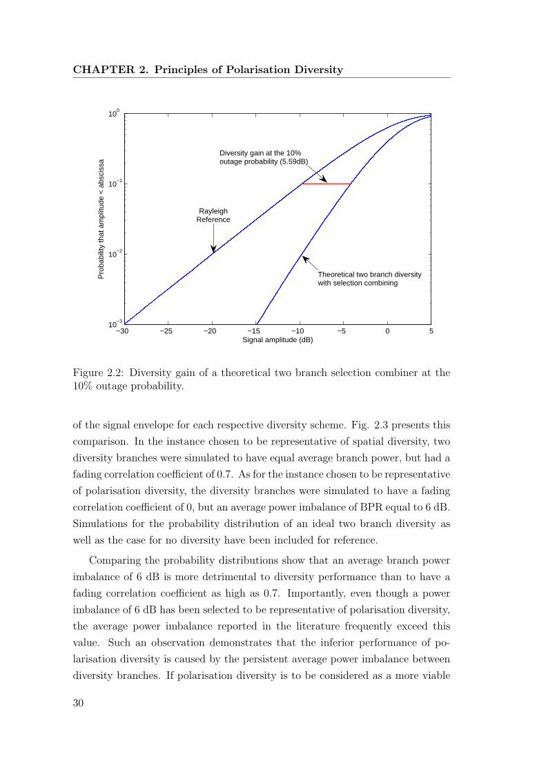
CHAPTER 2. Principles of Polarisation Diversity
−30 −25 −20 −15 −10 −5 0 510
−3
10−2
10−1
100
Signal amplitude (dB)
Pro
babi
lity
that
am
plitu
de <
abs
ciss
a
RayleighReference
Theoretical two branch diversitywith selection combining
Diversity gain at the 10%outage probability (5.59dB)
Figure 2.2: Diversity gain of a theoretical two branch selection combiner at the10% outage probability.
of the signal envelope for each respective diversity scheme. Fig. 2.3 presents this
comparison. In the instance chosen to be representative of spatial diversity, two
diversity branches were simulated to have equal average branch power, but had a
fading correlation coefficient of 0.7. As for the instance chosen to be representative
of polarisation diversity, the diversity branches were simulated to have a fading
correlation coefficient of 0, but an average power imbalance of BPR equal to 6 dB.
Simulations for the probability distribution of an ideal two branch diversity as
well as the case for no diversity have been included for reference.
Comparing the probability distributions show that an average branch power
imbalance of 6 dB is more detrimental to diversity performance than to have a
fading correlation coefficient as high as 0.7. Importantly, even though a power
imbalance of 6 dB has been selected to be representative of polarisation diversity,
the average power imbalance reported in the literature frequently exceed this
value. Such an observation demonstrates that the inferior performance of po-
larisation diversity is caused by the persistent average power imbalance between
diversity branches. If polarisation diversity is to be considered as a more viable
30

2.6 Addressing the power imbalance problem
−30 −25 −20 −15 −10 −5 0 510
−3
10−2
10−1
100
Signal amplitude (dB)
Pro
babi
lity
that
am
plitu
de <
abs
ciss
a
RayleighReference
Ideal twobranch diversity
BPR = 6dB
CorrelationCoefficient = 0.7
Figure 2.3: Comparison of performance between diversity schemes.
form of diversity, this average branch power imbalance must not be ignored.
2.6 Addressing the power imbalance problem
One method to address the power imbalance problem in polarisation diversity pro-
posed by Lukama [64] was to introduce an additional linearly polarised antenna
that is mounted orthogonal to the two existing polarisation diversity antennas. It
is true that with the extra diversity branch, some compensation may be achieved
for power imbalance, however, it does not fix the underlying problem.
Another technique to apply suitable gains to each diversity branch before
the diversity combiner for branch power equalisation was suggested by LeFevre
[57], Colburn [15], Green [36] and Sanchez [83]. These works do not explicitly
deal with the power imbalance problem of polarisation diversity, but do address
the more general problem of power imbalance between diversity branches. It
must be emphasised that this amplification procedure is not to be confused with
instantaneous power control, where the received envelopes at a particular instant
in time are amplified to have equal power. Here, only the average powers are
31

CHAPTER 2. Principles of Polarisation Diversity
amplified for average branch power equalisation. Even though equalisation can
be achieved in this way, the procedure must be exercised with caution. This is
because the amplification of a weak signal with a poor signal to noise ratio (SNR)
also raises the noise floor, which consequently introduces additional interference.
In the extreme case, amplification is counter productive and it is much better to
ignore the non contributing diversity branch.
By far the most effective solution to achieve suitable branch power balance
for polarisation diversity is the use of alternative antenna configurations at the
receiver to facilitate the capture of diversity signals with comparable power. This
concept was first propounded by Kozono in [48], who suggested the use of a
receiver antenna system with two linearly polarised elements aligned at angles
±α relative to the vertical axis instead of the traditional vertical and horizon-
tal alignment. Under high XPD situations, the geometric symmetry achieved by
such antenna placement promotes a better BPR since the power in the domi-
nant vertical polarisation is more easily distributed into the ±α antennas. This
equalisation technique was shown to be effective, at the cost of a slightly in-
creased fading correlation, which were measured to be in the order of 0.3 and
0.4. Control over the value of the correlation coefficient can be achieved with the
further modification of α. However, for α = 45◦, power loss is observed due to
polarisation misalignment.
Experimental work featuring this particular antenna configuration has been
explored extensively in publications such as [27, 28, 52, 53, 59, 69, 88, 99]. Perfor-
mance benefits over the traditional vertical and horizontal systems, especially in
high XPD scenarios, were frequently reported. For instance, Emmer [28] reports
that the diversity gain observed for the ±45◦ system was consistently 2 dB better
than the traditional vertical and horizontal polarisation system. Comparisons of
the RSSI and the grade of BER quality presented by Lempiainen [59] and Laiho-
Steffens [52, 53] show a slightly improved performance for the ±45◦ system. In
the urban areas of downtown Stockholm, Wahlberg [99] noted an additional 1 dB
diversity gain with the ±45◦ antenna alignment over the traditional vertical and
horizontal implementation. Narayanan [69] reports similar performance advan-
tages of 1.2 dB.
A comparison of the raw diversity parameters between the Kozono and tra-
ditional polarisation diversity implementations was made by Eggers in [27]. The
±45◦ antenna configuration was measured to exhibit an average branch power
32

2.7 Power imbalance and orientation sensitivity
difference of 1.6 dB, which is significantly better than the traditional vertical and
horizontal alignment, measured in the same study to be 7.6 dB. The fading cor-
relation coefficient, however, was reported to be insensitive to the variation, and
measured 0.09 for both cases.
In the three studies that were previously identified to exhibit unusually low
XPD values, [7, 45, 88], two of the authors, Sorensen [88] and Joyce [45] also
examined the use of the ±α polarisation diversity antenna configuration. Both
authors report that irrespective of the configuration used, there was no significant
difference in the performance between the two types. This is interesting, because
it verifies the speculations that power coupling and depolarisation may have been
very effective at these study locations.
Aside from the experimental work, modelling of the polarisation diversity
problem using and extending upon the ±α configuration has been equally popu-
lar. For instance, Vaughan in [97] considers an antenna alignment that is fixed at
right angles (±45◦) but are rotated about the x axis. Brown in [10] generalised
the Kozono configuration to include the joint rotation of the antenna elements.
Enhanced performance of direct sequence - code division multiple access (DS -
CDMA) using the Kozono antenna configuration was proposed by Correal [16].
Liang [61] investigated the incorporation of multi-input multi-output (MIMO)
with polarisation diversity as space effective alternatives to spatial diversity.
2.7 Power imbalance and orientation sensitivity
The number of publications that have chosen to proceed with the ±α configu-
ration is a testament to the popularity of the scheme. In the original antenna
configuration proposed by Kozono, the transmission of a principally vertically
polarised signal is assumed. However, in the mobile uplink where mobile orienta-
tion is typically random, the transmitted polarisation is not necessarily vertical,
and the symmetry between the transmitter and receiver units to facilitate power
redistribution between the diversity antennas is no longer preserved.
It can be argued that if the channel conditions continues to preserve a domi-
nating of the vertical polarisation the ±α antenna configuration would remain a
suitable diversity scheme, regardless of the transmitter polarisation. Conversely
if the channel were to be able guarantee signal depolarisation, the power bal-
ance problem is eliminated and use of either antenna configuration becomes im-
33

CHAPTER 2. Principles of Polarisation Diversity
material. The depolarisation properties of the channel is the mechanism that
ultimately dictates the effectiveness of polarisation diversity.
The evidence available in the literature, however, suggests that it is uncom-
mon for the channel be independent of the transmitter polarisation. Studies
investigating the effects of variable transmitter polarisation in both the tradi-
tional vertical-horizontal and Kozono’s ±α antenna configurations consistently
report on the variations of diversity performance as a function of the transmitter
polarisation. For example, Nakano [68] considers the transmitter orientations of
vertical (0◦), horizontal (90◦), and 60◦ in the traditional vertical and horizontal
polarisation diversity setup. The comparison demonstrates that while the diver-
sity gain of space diversity was better than polarisation diversity in the 0◦ and
90◦ orientations, polarisation diversity was better at an orientation of 60◦. A
similar investigation was conducted by Smith [87] with mobile units transmitting
with orientations 0◦, 45◦ and 90◦ from the vertical. It was reported that the hor-
izontal and vertical orientations gave the best and worst diversity performance
respectively, with 45◦ in between. The polarisation diversity antenna alignment
considered here was also of the traditional vertical and horizontal polarisation
configuration. In Lotse [63], a transmitter inclination of 70◦ from the vertical was
considered and compared against a reference vertical polarisation. It was found
that the tilted cases yielded diversity gains that were 1 dB to 2 dB higher than
the vertical cases. Consistent observations were reported by Narayanan [69], who
considers vertical and 45◦ orientations at the transmitter site. Different transmit-
ter orientations were tested for both the traditional and ±α polarisation diversity
schemes. The results demonstrate better diversity gains when transmitting with
the 45◦ orientation for both cases.
Turkmani [94] is an instance in the literature where polarisation diversity was
reported to be insensitive to various transmitter orientations. The experimental
apparatus was set up to capture polarisation diversity signals in the vertical and
horizontal planes, given different transmitter orientations of 0◦, 30◦, 45◦, 60◦, and
90◦ from the vertical axis. Despite the presented analysis emphasising orienta-
tion insensitivity, the experimental data as well as the way with which it was
presented suggests that the reader should approach the conclusions with caution
and scepticism. In all of the data that was collected and presented within the
paper (Table I and II), it is clear that the inclination of the transmitter antenna
played an important part in the power balance of the diversity system. Variations
34

2.7 Power imbalance and orientation sensitivity
in the value of the XPD can be as big as 12 dB following an orientation change of
45◦. Calculated diversity gains for the Huyton suburban area also demonstrates
a clear difference between the case of a vertical and 45◦ transmitter, which were
reported to be 2.3 dB and 5.1 dB respectively. The graphical presentation of
the data is also questionable, because if ideal theoretical diversity gains at the
10% outage probability is expected to be no greater than 6 dB, it is unclear why
the authors chose to represent this on a scale of 0 dB to 16 dB. The use of this
inappropriate scale diminishes the observable differences in diversity performance
when transmitter orientations are introduced.
The performance of polarisation diversity, as with other antenna diversity
techniques, depends on the fading correlation and the average power of the di-
versity branches. Polarisation diversity is generally at a disadvantage to space
diversity due to the large power imbalance if the vertical and horizontal polari-
sations are being used. Better power balance between diversity branches can be
achieved when particular antenna geometries are applied to introduce symmetry
between the transmitter and receiver units. The antenna symmetry, however,
may be difficult to maintain especially when random transmitter orientations
in the uplink and channel characteristics dictate the depolarisation behaviour.
Acceptable diversity performance for a specific antenna orientation may become
unsatisfactory following a change in the antenna orientations and disturbing the
antenna symmetry. Enhancing the performance of polarisation diversity and
ensuring its robust performance requires both the average BPR or the fading
correlation coefficient to be examined in light of variable antenna geometries and
orientations.
35


Chapter 3
Acceptable Bounds for Diversity
Parameters
Capturing diversity signals that have uncorrelated fading and equal average branch
power is necessary for any kind of diversity to function effectively. Quantitatively,
this translates to a power correlation coefficient equal to 0 and a branch power
ratio equal to 0 dB. The acceptable parameter bounds for diversity, as reviewed
in Chapter 2, require a power correlation coefficient below 0.7 and an average
branch power ratio below 6 dB. Failure to fulfil this requirement degrades com-
munications quality and increases the probability of losing a call.
The diversity parameters achieved by polarisation diversity fall within these
bounds, but are far from being ideal. While the power correlation coefficient
is usually close to zero, with values rarely exceeding 0.4, the average branch
power ratio is typically quite high and frequently exceeds the 6 dB limit. This is
especially true in the suburban and rural environments.
An investigation into exactly how non-ideal diversity systems would adversely
influence a communications system was the major motivation of this chapter.
The work presented in this chapter serves three objectives. Firstly, to emphasise
the importance of facilitating the capture of diversity signals that have low fad-
ing correlation and equal average branch power. Secondly to demonstrate that
suboptimal diversity conditions can lead to an overall deterioration in system
performance. Finally, to challenge the consensus of the 6 dB upper limit for an
acceptable average branch power ratio. The results of this research demonstrate
that this limit is far too high, and needs to be significantly reduced.
The asynchronous Multiple Carrier (MC)-CDMA is chosen to serve as an

CHAPTER 3. Acceptable Bounds for Diversity Parameters
example for this research. The rationale behind this choice was that the MC-
CDMA is a narrow band system, which is susceptible to multipath fading. MC-
CDMA, unlike broadband communications, does not inherently provide diversity
in the frequency domain, and requires the implementation of a separate diversity
system to alleviate multipath fading. Antenna polarisation diversity was chosen
as the system to perform this task.
The overview of this chapter is as follows. First, an introduction to MC-
CDMA is presented in Section 3.1. The reasons why separate diversity systems
should be implemented with the MC-CDMA is explained in more detail. The syn-
chronous and asynchronous cases of the MC-CDMA are explained in Sections 3.2
and 3.3 respectively. These sections introduce the mathematical notations for
MC-CDMA . This development is necessary to allow the formulation of a math-
ematically consistent model of polarisation diversity in the MC-CDMA frame-
work. Particular emphasis on the concept of multiple access interference were
also given in these two sections, as it is the key agent causing performance dete-
rioration when suboptimal polarisation diversity is applied. Section 3.4 formally
studies the application of polarisation diversity in asynchronous MC-CDMA. Per-
formance deterioration is quantified and examined from the perspective of sub-
optimal diversity parameters. Results presented here challenge the acceptable
performance bounds in current published literature. Finally, Section 3.5 con-
cludes the chapter.
3.1 The MC-CDMA scheme
The MC-CDMA was a candidate multiple access technique proposed for the
fourth generation (4G) mobile communication system. Its operation is based on
the combination of DS-CDMA and orthogonal frequency division multiplexing
(OFDM).
DS-CDMA is a spread spectrum multiple access technique that allows mul-
tiple users to simultaneously access and occupy a block of spectra at any given
moment. Individual users are assigned an unique binary pseudo random code
sequence, which possesses the wideband properties of white noise, but are orthog-
onal against all other sequences of different users. Application of this code occurs
across the time domain by modulating the code against user specific data. This
operation causes user signals to spread across the frequency domain and occupy
38

3.1 The MC-CDMA scheme
a bandwidth far greater than the original signal. Orthogonality is maintained
in the code domain, allowing multiple users to simultaneously use a transmis-
sion medium. Discrimination between different users at the receiver is performed
through the correlation procedure and only the data of the intended user will be
extracted.
One major limitation of the DS-CDMA is its susceptibility to excessive time
delays of the mobile channel. Transmitted symbols are broadened in time causing
them to overlap with adjacent pulses and causes intersymbol interference (ISI).
This is particularly problematic for DS-CDMA because the individual code sym-
bols, or code chips, have very short durations comparable to the channel delay
spread. Chip synchronisation also becomes difficult with the increase in data
rates.
Sensitivity of the DS-CDMA to excess time delay and ISI can be addressed
by combining its operation with the orthogonal frequency division multiplexing
(OFDM) technique.
OFDM is a multiple carrier modulation technique which transmits a single
serial data stream in parallel over a large number of overlapping narrowband
frequency subcarriers. The conversion from serial to parallel transmission, given
a fixed throughput, increases the duration of each symbol and suppresses any
smearing effects introduced by the excess channel delay spread. The challenges
of symbol synchronisation are also significantly simplified with extended symbol
durations.
The multiple parallel OFDM subcarriers are usually designed to overlap in
the frequency domain, providing a framework which achieves very high levels of
spectral efficiency. Fig. 3.1 illustrates an example of the overlapping OFDM
subcarriers. Subcarrier orthogonality is preserved over the entire duration of
the symbol when the frequency separation is maintained at integer multiples of
1/Ts, where Ts is the symbol duration. The use of narrowband subcarriers also
avoids the need for complex frequency equalisation, allowing the assumption of
frequency flat fading conditions [103].
The OFDM is also attractive because the modulator and demodulator stages
can be implemented efficiently with the fast Fourier transform (FFT) algorithms.
Its flexibility and scalability allows higher data rates without substantially in-
creasing the system complexity.
The OFDM, however, is a digital modulation scheme for a single user, and not
39

CHAPTER 3. Acceptable Bounds for Diversity Parameters
0 1 2 3 4 5 6 7 8 9 10
−0.2
0
0.2
0.4
0.6
0.8
1
Frequency (Hz)
Am
plitu
de
Figure 3.1: Overlapping OFDM frequency subcarriers.
designed to be a multiple access technique. Combining OFDM and DS-CDMA to
form MC-CDMA is one possibility to enable multiple access and simultaneously
address the limitations of both schemes. That is, the frequency selectivity and
synchronisation problems of DS-CDMA are addressed using OFDM by increasing
individual chip durations without compromising data throughput, while multi-
ple access with OFDM is enabled with DS-CDMA, allowing the simultaneous
occupation of frequency subcarriers by multiple users.
Though the combination of OFDM and DS-CDMA presents an advanta-
geous mode of multiple access, MC-CDMA does inherit problems of both parent
schemes and introduces new challenges. Limitations derived from OFDM in-
clude sensitivity to intercarrier interference (ICI) and high peak-to-average power
(PAP) ratios. ICI is the interference produced when OFDM subcarriers lose or-
thogonality and causes energy within a particular subcarrier to leak into adjacent
subcarriers. Suppression of ICI can be achieved with better subcarrier synchro-
nisation, or through the appropriate insertion of guard time intervals [102].
High PAP ratios arise when the set of independently modulated subcarriers
are summed coherently to produce a large peak in the instantaneous power. The
40

3.1 The MC-CDMA scheme
immediate disadvantage is the strain imposed on the RF amplifiers to operate
over such a wide dynamic range [66]. In the event that the RF amplifiers reach
saturation, signal clipping occurs and the peak amplitude becomes limited to
some maximum level. This distortion can be regarded as a multiplication of the
OFDM symbol with a rectangular window in the time domain, causing significant
amounts of energy to leak into adjacent frequency bands as a consequence of the
convolution in the frequency domain [78]. Interference of this kind can be subdued
with precoding methods to ensure that subcarriers do not sum coherently, or with
the application of pulse shaping to reduce out-of-band radiation caused by signal
clipping.
A limitation of the MC-CDMA derived from the DS-CDMA is its vulnera-
bility to the loss of orthogonality between user codes. This type of interference
is called multiple access interference (MAI). MAI can severely degrade signal
quality and is the main factor that determines the capacity of the system. MAI
is especially problematic in the mobile uplink because communication occurs in
an asynchronous manner. Different time delays between individual users do not
allow code sequences to maintain orthogonality.
A new challenge resulting from the combination of OFDM and DS-CDMA is
the need for additional signalling diversity. The application of the OFDM with
DS-CDMA transforms a wideband frequency equalisation problem into a narrow-
band multipath fading problem. Effects of multipath fading are best alleviated
using diversity techniques. Inherently, the OFDM is capable of supporting fre-
quency diversity with the dynamic allocation of additional subcarriers, at the
cost of some system capacity. However, for MC-CDMA, this dynamic allocation
is not easily achieved since user specific spreading codes have already been as-
signed across the frequency domain. For this reason, it is necessary to examine
alternative forms of diversity to counteract narrowband fading, such as antenna
polarisation diversity.
The application of antenna diversity alleviates the effects of fading by min-
imising the occurrence of deep fades and increasing the average carrier to noise
ratio (CNR). However, when applied with MC-CDMA, an improvement in the
CNR does not automatically translate into an improvement in system perfor-
mance. This is because antenna diversity indiscriminately captures both signal
and interference. The extra diversity path can lead to proportionately increased
interference, especially if equal average power between diversity branches can not
41

CHAPTER 3. Acceptable Bounds for Diversity Parameters
be maintained. The application of diversity in the presence of MAI is not well
documented in the literature. Existing parameter bounds that are established as
prerequisites for acceptable diversity assumes the absence of MAI. It is therefore
of interest to investigate the possibility of performance deterioration due to un-
intentional introduction of additional MAI through diversity. In fact, the results
found through this research challenges the validity of existing parameter bounds
for diversity.
The next two sections establish the mathematical framework and notations for
the MC-CDMA system. The synchronous MC-CDMA system is examined first
and will then be generalised into an asynchronous MC-CDMA system. The two
different types of multiple access interference, which are key variables in studying
of the adverse effects of suboptimal diversity, have been derived in the process.
These developments are necessary to demonstrate that the application of polar-
isation diversity to asynchronous MC-CDMA does not always give favourable
results.
3.2 Synchronous MC-CDMA
The synchronous MC-CDMA system is illustrated in Fig. 3.2. At the transmitter
side, there are a total of N active users, each of whom has data which needs to
be sent. The kth individual, has data represented by bk, and is assumed to be
a binary phase shift keying (BPSK) modulated waveform. In preparation for
the MC-CDMA modulator, data from a particular user is first replicated across
parallel subcarriers. The number of parallel branches required depends on the
spreading factor of the user code. Here, the number of subscribers has been
assumed to equal the spreading factor of the user codes. Such systems are said
to be operating at full capacity.
Application of the user codes occurs after replicating bk across the N parallel
subcarriers, with the ith chip of the user code being assigned to the ith subcar-
rier. For example, given the kth user with code sequence {Ck,1, Ck,2, · · · , Ck,N},subcarrier branch fk,1 is assigned with chip Ck,1, subcarrier branch fk,2 is assigned
with chip Ck,2, and so forth for all N subcarriers.
Each of the N subcarriers are then modulated to its assigned frequency with
the multiplication of cos (2πfit) and summed, before being transmitted through
the channel. This conversion from a serial chip stream into parallel transmission
42

3.2 Synchronous MC-CDMA
User k
MC-CDMA Transmitter
User 2
MC-CDMA Transmitter
bk
b2
User 1
b1
×
C1,1
C1,N
×
×
C1,2
×
×
×
cos (2πf1t)
cos (2πf2t)
cos (2πfN t)
+
+
Channel
s (t) r (t)
×
×
×
Cr,N
Cr,2
Cr,1
×
×
×
cos (2πfN t)
cos (2πf2t)
cos (2πf1t)
×
×
×
µr,N
µr,2
µr,1
+Ts∫0
dt
br (t)
Reference User Receiver
Figure 3.2: The synchronous MC-CDMA
increases the chip duration to equal the symbol duration, and suppresses the
adverse pulse smearing effects as a result of the excess channel delay spread. A
greater system tolerance against ISI is achieved.
The transmitted signal of the kth user, sk can be represented mathematically
as
sk (t) =N∑i=1
√2PbkCk,i cos (2πfit) . (3.1)
All subcarriers are assumed to carry equal power P , and all users are assumed
to be in complete time synchronisation. The combined signal from all users s (t)
equals the summation of sk (t), over k, for all N .
s (t) =N∑k=1
N∑i=1
√2PbkCk,i cos (2πfit) (3.2)
The channel model applied is a slow and frequency flat complex Gaussian
43

CHAPTER 3. Acceptable Bounds for Diversity Parameters
multipath fading channel. It is slow in the sense that the channel conditions are
assumed to remain constant over the duration of at least two symbol periods.
The channel for the ith subcarrier of the kth user, Hk,i, is expressed in polar
form as
Hk,i = Γk,iejθk,i , (3.3)
with the envelope fluctuations as a consequence of multipath fading represented
by Γ, and the random phase shift induced by the channel expressed by θ. Ap-
plication of the narrowband fading channel is performed with the multiplication
of Hk,i and s (t). The channel also introduces an additive white Gaussian noise
(AWGN) component nk,i. These are also assigned and added to each subcarrier
of every user.
Signals captured by the receiver antenna r (t) immediately after the channel
is expressed mathematically as
r (t) =N∑k=1
N∑i=1
√2PΓk,ibkCk,i cos (2πfit+ θk,i) + nk,i . (3.4)
Signal detection at the MC-CDMA receiver for a particular reference user
begins with replicating the received signal over N subcarriers. Subcarriers are de-
spread and demodulated individually with the multiplication of Cr,i and cos (2πfit).
The r subscript in Cr,i is used to identify the reference user.
Following the demodulation procedure, a gain coefficient µk,i is then applied
to each subcarrier to suppress the MAI. These gain coefficients are calculated by
first decomposing the test statistic Z at the output of the correlation receiver
into three parts,
Z =
∫ Ts
0
N∑i=1
r (t)µr,iCr,i cos (2πfit) dt (3.5)
=D + I + η , (3.6)
where D is the desired signal component, I is the interference from MAI, and η
44
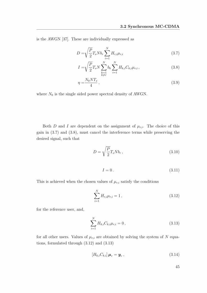
3.2 Synchronous MC-CDMA
is the AWGN [37]. These are individually expressed as
D =
√P
2TsNbr
N∑i=1
Hr,iµr,i (3.7)
I =
√P
2TsN
N∑k=1k =r
bk
N∑i=1
Hk,iCk,iµr,i , (3.8)
η =N0NTs
4, (3.9)
where N0 is the single sided power spectral density of AWGN.
Both D and I are dependent on the assignment of µr,i. The choice of this
gain in (3.7) and (3.8), must cancel the interference terms while preserving the
desired signal, such that
D =
√P
2TsNbr , (3.10)
I = 0 . (3.11)
This is achieved when the chosen values of µr,i satisfy the conditions
N∑i=1
Hr,iµr,i = 1 , (3.12)
for the reference user, and,
N∑i=1
Hk,iCk,iµr,i = 0 , (3.13)
for all other users. Values of µr,i are obtained by solving the system of N equa-
tions, formulated through (3.12) and (3.13)
[Hk,iCk,i]µr = yr , (3.14)
45

CHAPTER 3. Acceptable Bounds for Diversity Parameters
where [Hk,iCk,i] is the element by element product of Hk,i and Ck,i,
[Hk,iCk,i] =
H1,1C1,1 H1,2C1,2 . . . H1,iC1,i . . . H1,NC1,N
H2,1C2,1 H2,2C2,2 . . . H2,iC2,i . . . H2,NC2,N
......
. . .... . . .
...
Hr,1Cr,1 Hr,2Cr,2 . . . Hr,iCr,i . . . Hr,NCr,N
...... . . .
.... . .
...
HN,1HN,1 HN,2CN,2 . . . HN,iCN,i . . . HN,NCN,N
, (3.15)
and µr is the column vector of µr,i gains across all subcarriers for a particular
reference user. yr is a sparse vector with a single non-zero element at the rth
index, which is equal to 1. Assuming that [Hk,iCk,i] is non degenerate, the solution
to the system of equations is
µr = [Hk,iCk,i]−1 yr . (3.16)
The BER performance of two synchronous MC-CDMA systems are simulated
to demonstrate the MAI cancellation procedure. In one of the systems, MAI can-
cellation was not applied and the output of the demodulator stage was connected
directly into the bit detection stage. In a separate system, values of µr were
calculated and assigned to cancel the MAI interference. The BER performance
of these two systems are illustrated in Fig. 3.3. With the application of MAI
cancellation, the BER can be reduced from 10−1.7 to 10−4 at an SNR of 30 dB.
This result is evidence that MAI cancellation is mandatory for the successful
operation of synchronous MC-CDMA.
The results in Fig. 3.3 were obtained through the simulation of a 16 user
synchronous MC-CDMA operating at full capacity. Ten million independent trials
were used to calculate the BER as a function of the SNR. Each user is assumed
to be subject to an independent set of 16 complex Gaussian channels, which are
assigned to individual frequency subcarriers. Signal fading affecting subcarriers
for any individual user is assumed to be highly correlated since the spectral
separation between overlapping subcarriers is significantly less than the coherence
bandwidth. The fading correlation coefficient between subcarriers were set to 0.7
in order to reflect this condition. Correlated fading channels were generated using
the algorithm presented in [89] based on the Cholesky decomposition technique.
In this section, operation of the synchronous MC-CDMA was examined. The
46

3.2 Synchronous MC-CDMA
0 5 10 15 20 25 3010
−4
10−3
10−2
10−1
100
SNR (dB)
Bit
Err
or R
ate
µr=[H
k,iC
k,i]−1y
r
µr=1
Figure 3.3: Comparison of the BER between synchronous MC-CDMA systemsusing equal gains and MAI cancellation gains
.
mathematical framework has been established and expressions for the relevant
variables presented. In particular, expressions for the test statistic, its decom-
position into the desired, interference and AWGN components as well as the µr
user weights were derived. Performance of the synchronous MC-CDMA was also
simulated and presented.
In the next section, the asynchronous case of the MC-CDMA is established
through the generalisation of the synchronous MC-CDMA. The asynchronous
MC-CDMA occurs in the mobile uplink when timing offsets between different
users cause user codes to lose orthogonality. Expressions for the two different
kinds of MAI are derived, and shown that they cannot be eliminated with µr.
This interference is the principal cause the performance deficit when an additional
poorly performing diversity branch is introduced, the details of which will be
examined in Section 3.4.
47

CHAPTER 3. Acceptable Bounds for Diversity Parameters
User k
MC-CDMA Transmitter
User 2
MC-CDMA Transmitter
b1
bk
b2
User 1
×
C1,N
×
cos (2πfN t)
×
×
C1,1
C1,2
×
×
cos (2πf1t)
cos (2πf2t)
+
Delayτk
Delayτ2
Delayτ1
+s (t)
Channel
r (t)
×
×
×
Cr,1
Cr,2
Cr,N
×
×
×
cos (2πf1t)
cos (2πf2t)
cos (2πfN t)
×
×
×
µr,1
µr,2
µr,N
+Ts∫0
dt
br (t)
Base Station Receiver
Demodulating the Reference User
Figure 3.4: The asynchronous MC-CDMA. User delays τk are introduced imme-diately after the transmitter stage of each user.
3.3 Asynchronous MC-CDMA
Communications occurs in an asynchronous manner in the mobile uplink. Even
though users are synchronised to the base station, the time delays introduced
from the different propagation distances causes the signals from different users to
fall out of synchronisation.
User specific time delays, τk, are introduced at the transmitter side to account
for these timing discrepancies. Perfect synchronisation is assumed for the refer-
ence user with τr set to zero, and delays from all other N − 1 users evaluated
against this reference. The asynchronous MC-CDMA is illustrated in Fig. 3.4.
The structure of asynchronous MC-CDMA receiver is identical to the syn-
chronous case. However, with the introduced time delays, the expressions for
the combined signal from all users, s (t), and the signal captured by the receiver
48

3.3 Asynchronous MC-CDMA
antenna immediate after the channel, r (t), become,
s (t) =N∑k=1
N∑i=1
√2Pbk (t− τk)Ck,i cos (2πfi (t− τk)) , (3.17)
r (t) =N∑k=1
N∑i=1
√2PΓk,ibk (t− τk)Ck,i cos (2πfi (t− τk) + θk,i) + nk,i. (3.18)
Demodulation continues with the replication of r (t), over N parallel subcarriers
followed by the multiplication of Cr,i cos (2πfit)µr,i. The subcarriers are then
summed and input into the correlator, where the resultant output Z can be
calculated as a summation of a desired component D, a MAI component I and
an AWGN component η.
Z =
∫ Ts
0
N∑i=1
r (t)µr,iCr,i cos (2πfit) dt (3.19)
=D + I + η . (3.20)
The expressions D and η for the asynchronous MC-CDMA remain identical to
the expressions of D and η in the synchronous MC-CDMA, and are calculated as
D =
√P
2TsNbr
N∑i=1
Γr,iµr,i , (3.21)
η =N0NTs
4. (3.22)
The expression for I, however, it is now calculated as
I =II + IJ , (3.23)
II =
√P
2
K∑k=1k =r
N∑i=1
µr,iCk,iCr,i cos (θk,i)
· [Γk,i (−1) bk (−1) τk + Γk,i (0) bk (0) (Ts − τk)] , (3.24)
49

CHAPTER 3. Acceptable Bounds for Diversity Parameters
IJ =
√P
2
K∑k=1k =r
N∑i=1
N∑j=1j =i
µr,iCk,jCr,i
2π (i− j)· [Γk,j(−1)bk(−1)− Γk,j(0)bk(0)]
·[sin
(2π(i− j)τk
Ts+ θk,j
)− sin (θk,j)
]. (3.25)
The new MAI expression I accounts for a different type of MAI that emerges
with the loss of orthogonality between user codes caused by asynchronous timing
offsets. This expression for I consists of two parts, II and IJ , which represent
the same carrier and different carrier interference terms respectively [37]. The
formulation of II and IJ require both the current and previous transmission time
intervals be taken into account, and are identified with the (0) and (−1) time
indices respectively.
In the asynchronous case, it is impossible to select suitable values of µr which
can simultaneously eliminate interference contributions from both transmission
intervals. Partial MAI suppression, however, can still be achieved by calculating
µr with (3.16) using the conditions of the current time interval.
The Simulated performance of the asynchronous MC-CDMA is illustrated in
Fig. 3.5. Its BER as a function of the SNR has been plotted in red. The perfor-
mance of the asynchronous MC-CDMA without MAI cancellation and the syn-
chronous MC-CDMA were also plotted for comparison. The results demonstrate
that correct application of the MAI cancellation term µr, allows an improvement
for the BER with a reduction from 10−1.7 to 10−3 at an SNR of 30 dB. However,
since MAI can not be completely eliminated in the asynchronous MC-CDMA,
the BER is considerably higher than the 10−4 at SNR 30 dB achievable by the
synchronous MC-CDMA.
The parameters used for the performance simulation were identical to Section
3.2, and assumes the 16 user MC-CDMA operating at full capacity. Fading
effects were assumed independent between users but correlated with a coefficient
of 0.7 between subcarriers. The timing delay introduced in the asynchronous
communications τk, is treated as independent and identically distributed (i.i.d.),
and uniformly distributed between 0 and Ts.
The asynchronous nature of the MC-CDMA uplink introduces timing dis-
crepancies between users which creates a new form of MAI as user codes lose
orthogonality. The MAI cancellation gains, µr, established in the synchronous
case are shown to be ineffective here. Complete elimination of the MAI in the
50

3.4 Asynchronous MC-CDMA with polarisation diversity
0 5 10 15 20 25 3010
−4
10−3
10−2
10−1
100
SNR (dB)
Bit
Err
or R
ate
Asyn MCCDMA without MAI cancellationAsyn MCCDMA with MAI cancellationSynchronous Reference
Figure 3.5: BER performance of the asynchronous MC-CDMA. Cases of theasynchronous MC-CDMA with and without MAI cancellation are compared. Thestandard synchronous MC-CDMA has been included for reference.
asynchronous case is demonstrated to be impossible using this technique. The
implication of this is that the additional layer of diversity needs to be applied with
caution as diversity techniques do not discriminate between signal and interfer-
ence. Any improvements in the carrier to noise ratio would not automatically
imply a decreased BER.
In the next section, the performance deficit when polarisation diversity is
applied to asynchronous MC-CDMA is presented. These results challenge the
existing parameter bounds considered acceptable for diversity action.
3.4 Asynchronous MC-CDMAwith polarisation
diversity
The antenna polarisation diversity scheme is vulnerable to the power imbalance
condition. The review of the literature identified that signals received in the hor-
izontal polarisation can be consistently lower than the vertical polarisation. This
power imbalance is problematic in the framework of the asynchronous MC-CDMA
51

CHAPTER 3. Acceptable Bounds for Diversity Parameters
MC-CDMA
Transmitter
sr (t)
MC-CDMA
Receiver
MC-CDMA
Receiver
rv (t)
rh (t)
Hv,r,i
Hh,r,i
+
Zv
Zh
br (t)
Figure 3.6: Asynchronous MC-CDMA with polarisation diversity. Here, theMC-CDMA receiver consists of two parallel stages, one for each of the verticaland horizontal polarisations. Signal demodulation is performed independently,and the output test statistics are combined before bit detection. The transmitterstage is identical to the one in Section 3.3, however for clarity purposes, only thesignal contribution from the reference user sr (t) has been drawn.
because diversity paths with weak signal contribution will introduce proportion-
ally more interference. This section demonstrates the performance penalties as
a result of this power imbalance condition and challenges the validity of existing
parameter bounds for acceptable diversity action.
The asynchronous MC-CDMA system with polarisation diversity is illustrated
in Fig. 3.6. The structure of the MC-CDMA transmitter is identical to the one
in Section 3.3. The transmitted signal, expressed as
s (t) =N∑k=1
N∑i=1
√2Pbk (t− τk)Ck,i cos (2πfi (t− τk)) , (3.26)
are assumed to be transmitted through a vertically polarised antenna.
EM wave propagation through the mobile channel occurs in a multipath man-
ner. Interactions with the channel obstacles along the propagation route causes
signal depolarisation, where some of the signal power originally concentrated in
the vertical polarisation is transferred into the horizontal polarisation. It is this
depolarisation mechanism that allows antenna polarisation to be a mode of di-
versity.
Empirical treatment of polarisation channels in the literature shows both the
vertical and horizontal polarisations to be well modelled by complex Gaussian
channels, expressed in polar form as
Hh,k,i = Γh,k,iejθh,k,i , (3.27)
Hv,k,i = Γv,k,iejθv,k,i , (3.28)
52

3.4 Asynchronous MC-CDMA with polarisation diversity
with Γ representing the small scale fading and θ, the random phase offsets induced
by channel. Subscripts v and h indicate the vertical and horizontal polarisations
respectively. The orthogonal polarisations generally exhibit very low levels of
fading correlation, but not equal power. It is rare for correlation coefficients to
be take values larger than 0.4, but a difference between average branch power is
common and can be as high as 6 dB. The metric used to quantify the level of
power imbalance is the XPD, defined as the power ratio of the vertical polarisation
with respect to the horizontal polarisation,
XPD =E[Γ2v,k,i
]E[Γ2h,k,i
] . (3.29)
The depolarisation phenomenon is performed mathematically as the multiplica-
tion of Hv,k,i and Hh,k,i against s(t). The resultant signals in the vertical rv (t)
and horizontal rh (t) polarisations are calculated as
rv (t) =N∑k=1
N∑i=1
√2PΓv,k,ibk (t− τk)Ck,i cos (2πfi (t− τk) + θv,k,i) + nv,k,i ,
(3.30)
rh (t) =N∑k=1
N∑i=1
√2PΓh,k,ibk (t− τk)Ck,i cos (2πfi (t− τk) + θh,k,i) + nh,k,i.
(3.31)
A standard polarisation diversity receiver front end with antennas aligned along
the vertical and horizontal polarisations was used to independently capture these
signals. Such an antenna alignment means the power imbalance of the XPD
translates directly into the BPR.
Each antenna is attached to its own standard MC-CDMA receiver, indepen-
dently despreading and demodulating the captured signals. Test statistics Zv
and Zh for the vertical and horizontal polarisations generated at the output of
53
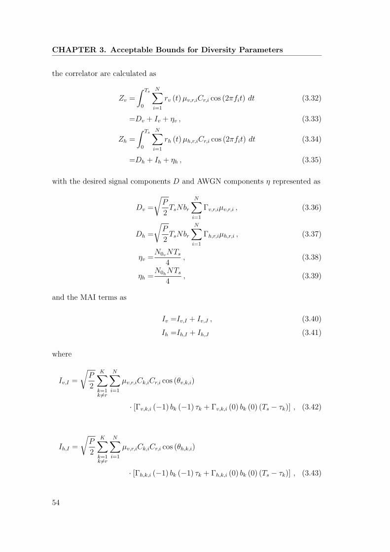
CHAPTER 3. Acceptable Bounds for Diversity Parameters
the correlator are calculated as
Zv =
∫ Ts
0
N∑i=1
rv (t)µv,r,iCr,i cos (2πfit) dt (3.32)
=Dv + Iv + ηv , (3.33)
Zh =
∫ Ts
0
N∑i=1
rh (t)µh,r,iCr,i cos (2πfit) dt (3.34)
=Dh + Ih + ηh , (3.35)
with the desired signal components D and AWGN components η represented as
Dv =
√P
2TsNbr
N∑i=1
Γv,r,iµv,r,i , (3.36)
Dh =
√P
2TsNbr
N∑i=1
Γh,r,iµh,r,i , (3.37)
ηv =N0vNTs
4, (3.38)
ηh =N0hNTs
4, (3.39)
and the MAI terms as
Iv =Iv,I + Iv,J , (3.40)
Ih =Ih,I + Ih,J (3.41)
where
Iv,I =
√P
2
K∑k=1k =r
N∑i=1
µv,r,iCk,iCr,i cos (θv,k,i)
· [Γv,k,i (−1) bk (−1) τk + Γv,k,i (0) bk (0) (Ts − τk)] , (3.42)
Ih,I =
√P
2
K∑k=1k =r
N∑i=1
µv,r,iCk,iCr,i cos (θh,k,i)
· [Γh,k,i (−1) bk (−1) τk + Γh,k,i (0) bk (0) (Ts − τk)] , (3.43)
54

3.4 Asynchronous MC-CDMA with polarisation diversity
and
Iv,J =
√P
2
K∑k=1k =r
N∑i=1
N∑j=1j =i
µv,r,iCk,jCr,i
2π (i− j)· [Γv,k,j(−1)bk(−1)− Γv,k,j(0)bk(0)]
·[sin
(2π(i− j)τk
Ts+ θv,k,j
)− sin (θv,k,j)
], (3.44)
Ih,J =
√P
2
K∑k=1k =r
N∑i=1
N∑j=1j =i
µh,r,iCk,jCr,i
2π (i− j)· [Γh,k,j(−1)bk(−1)− Γh,k,j(0)bk(0)]
·[sin
(2π(i− j)τk
Ts+ θh,k,j
)− sin (θh,k,j)
]. (3.45)
Importantly, application of the MAI cancellation coefficients µv,r and µh,r are
polarisation specific and need to be calculated using the channel conditions of
the current transmission interval.
µv,r = [Hv,k,i (0)Ck,i]−1 yr (3.46)
µh,r = [Hh,k,i (0)Ck,i]−1 yr (3.47)
Finally, at the bit detection stage, test statistics Zv and Zh are combined by
means of a sum and input into the decision device.
The simulated BER performance of the asynchronous MC-CDMA with polar-
isation diversity under different levels of power imbalance is presented in Fig. 3.7.
The results shows firstly, that if polarisation diversity branches are power bal-
anced, the performance of the asynchronous MC-CDMA can be improved with a
reduction in the BER. The BER was recorded to be 4×10⁻⁵ for a SNR of 30 dB, a
significant improvement over the BER of 2× 10⁻³ for the standard asynchronous
MC-CDMA with no diversity.
The second observation is that system performance degrades quickly with
power imbalance, clearly demonstrating that if the average branch between di-
versity branches cannot be balanced, system performance worsens with diversity.
Performance penalties occur with power imbalances as small as 3 dB, and is
attributed to the indiscriminate capture of signal and interference by diversity
branches. Without sufficient contribution into fading rejection, the additional
55

CHAPTER 3. Acceptable Bounds for Diversity Parameters
0 5 10 15 20 25 3010
−5
10−4
10−3
10−2
10−1
100
SNR (dB)
Bit
Err
or R
ate
XPD=0dBXPD=3dBXPD=6dBXPD=9dBNo Diversity
Figure 3.7: BER performance of asynchronous MC-CDMA with polarisation di-versity, under different levels of branch power imbalance. Performance of thestandard asynchronous MC-CDMA without diversity is included for reference.
diversity branch serve as a source of interference and disrupts signal detection.
The parameters used to simulate the asynchronous MC-CDMA with polari-
sation diversity assumes 16 users and operates at full capacity. For each user, a
set of fading channels is generated for each of the polarisation branches. Signal
fading is assumed to be independent between users and independent between po-
larisations, but remain highly correlated between the carriers of each user, with
the correlation coefficient set at 0.7. Values of 0 dB, 3 dB, 6 dB and 9 dB were
assigned to the XPD in order to examine the effects of branch power imbalance
on the system performance. The simulation conducted ten million independent
trials for each value of the XPD.
3.5 Summary
The validity of existing parameter bounds for effective diversity were examined
through the example of using traditional polarisation diversity with MC-CDMA.
The established acceptable diversity parameters were challenged on the basis that
existing bounds were established in the absence of additional interference such
56

3.5 Summary
as MAI. Implementing diversity improves the CNR by minimising the duration
and occurrence of deep fades, but indiscriminately captures both signal and in-
terference. An improvement in the CNR does not therefore imply an automatic
improvement in performance.
This research evaluates the validity of acceptable bounds with empirical sim-
ulations of a 16 user asynchronous MC-CDMA system operating at full capacity.
Results demonstrate that significant improvements in the BER can be achieved
if ideal diversity conditions with uncorrelated fading and equal average branch
powers are available for diversity action. This shows that there is an overall sys-
tem performance improvement when optimum diversity is achieved, even if the
extra diversity branch had introduced more MAI.
Conditions for optimum function of diversity, however, are not typically achiev-
able with the standard traditional polarisation diversity. Average power imbal-
ances between the vertical and horizontal polarisations are consistently observed
to be in excess of 6 dB. Simulations show that BER performance degrades quickly
in the presence of power imbalance. In fact, performance deficits occur with an
average power imbalance as small as 3 dB. This result is significant because it
shows definitively that having no diversity is better than an under performing
diversity system. Such research outcomes is evidence that a proper implemen-
tation of polarisation diversity necessarily requires diversity branches to capture
diversity signals have zero fading correlation and equal average branch power.
57


Chapter 4
Model of the Generalised
Polarisation Diversity System
The average power imbalance between diversity branches is one of the major lim-
itations of polarisation diversity. Average branch power between the diversity
branches depends mainly on the polarisation of the transmitted signal, the orien-
tation of the transmitter and receiver terminals, and the channel. Existing work
in the literature presents only an elementary analysis into specific symmetric an-
tenna geometries, and does not provide a detailed analysis into the variability of
diversity parameters caused by antenna orientations.
This chapter presents a generalised mathematical framework for polarisation
diversity that describes the average branch power imbalance and power corre-
lation coefficient as a function of both the transmitter and receiver terminals.
Expressions for the branch power ratio and power correlation coefficient derived
here are applicable to any generic polarisation diversity system that uses two or-
thogonally mounted linearly polarised antennas at the transmitter and receiver.
This model can be simplified to account for traditional implementations of po-
larisation diversity, and can also be extended to investigate performance of po-
larisation diversity using the transmission of circularly and elliptically polarised
signals. Unlike much of the published literature which often assumes uncorrelated
diversity branches to simplify calculations, this model maintains generality with
correlated diversity branches. This is extremely important as the further perfor-
mance improvement of polarisation diversity by optimising the power correlation
coefficient in Chapter 7 would not be possible.
Subsequent chapters of the thesis, especially Chapters 5, 6 and 7, will be using

CHAPTER 4. Model of the Generalised Polarisation DiversitySystem
x
y
V1
V2
α
Transmitter
Figure 4.1: Generalised model of the transmitter component.
this polarisation diversity model extensively.
4.1 System model
The general model describes the polarisation diversity system in three compo-
nents, the transmitter unit, the polarisation channel and the polarisation diversity
receiver.
4.1.1 Transmitter component
The transmitter unit is modelled as a device with an antenna structure that
consists of two linearly polarised antenna elements V1 and V2 mounted in an
orthogonal manner. Each antenna is injected with a complex carrier of frequency
ω, and is written as
U =
[V1
V2
]=
[A1e
jωt
A2ej(ωt−θ)
]. (4.1)
The amplitudes of each respective complex carrier are represented by A1 and
A2. The phase difference between V1 and V2 is described by θ. In general, this
transmitted signal is elliptically polarised, but appropriate values can be assigned
to A1, A2 and θ to generate linearly polarised or circularly polarised signals.
This pair of transmitting antennas are assumed to be able to rotate in the xy
plane, as illustrated in Fig. 4.1. The angle of rotation is represented by α, and
is defined as the clockwise angle subtended from the vertical y axis to antenna
60

4.1 System model
Hpol
Vpol Vpol
HpolH11
H22
H12
H21
Figure 4.2: Generalised model of the polarisation diversity receiver.
V1. Projecting the signals from V1 and V2 into the horizontal Vx and vertical Vy
polarisations accounts for the transmitter orientation. This is achieved with the
multiplication of U by a transformation matrix, calculated as
V =
[Vx
Vy
]=
[sin (α) − cos (α)
cos (α) sin (α)
][V1
V2
]. (4.2)
4.1.2 Polarisation channel
The second component is the polarisation channel, it is modelled as a 2 by 2
matrix whose elements are complex Gaussian random variables [55, 63, 70], and
written as,
H =
[H11 H12
H21 H22
]=
[Γ11e
jϕ11 Γ12ejϕ12
Γ21ejϕ21 Γ22e
jϕ22
]. (4.3)
Each element of the H matrix describes the interactions between the vertical
and horizontal polarisations. A graphical representation of this interaction is
illustrated in Fig. 4.2. The elements H11 and H22 along the main diagonal
represent the co-polar links between the horizontal to horizontal and vertical to
vertical polarisations respectively. Elements along the anti-diagonal, H21 and H12
represent the cross-polar links between the vertical to horizontal and horizontal to
vertical polarisations. When expressed in polar form, Γmn represents the envelope
fading, and is Rayleigh distributed with power E [Γ2mn]. The envelope fading
between the Γ11 and Γ21 polarisation links as well as the Γ22 and Γ12 polarisation
links are assumed to be correlated. All other combinations of Γ are regarded as
independent. The ϕmn variables represent phase offsets induced by the channel,
and are all independent random variables uniformly distributed between [0, 2π).
Signal propagation through the polarisation channel is modelled with the mul-
61

CHAPTER 4. Model of the Generalised Polarisation DiversitySystem
x
y
R1
R2
ψ
Receiver
Figure 4.3: Generalised model of the polarisation diversity receiver.
tiplication of V by H. The resultant signal residing within the horizontal Rx and
vertical Ry polarisations immediately prior to reception is calculated as,[Rx
Ry
]=
[Γ11e
jϕ11 Γ12ejϕ12
Γ21ejϕ21 Γ22e
jϕ22
][Vx
Vy
]. (4.4)
4.1.3 Polarisation diversity receiver
The polarisation diversity receiver is the final component of the system. It is also
modelled as a device with two linearly polarised antennas R1 and R2 mounted
in an orthogonal manner, and allowed to rotate in the xy plane. The angle ψ
is used to describe the orientation of the receiver antenna, and is defined to be
the clockwise angle subtended between antenna R1 and the vertical y axis. A
diagram illustrating the structure of the receiver antenna system is illustrated in
Fig. 4.3. Signals captured by the diversity receiver are calculated by projecting
the Rx and Ry components after signal propagation into antennas R1 and R2,
written as, [R1
R2
]=
[sin (ψ) cos (ψ)
− cos (ψ) sin (ψ)
][Rx
Ry
]. (4.5)
62

4.2 Diversity parameters
4.2 Diversity parameters
The two parameters which dictate the performance of diversity systems are the
fading correlation coefficient and the branch power ratio (BPR). The objective is
to obtain generalised expressions for the BPR and the correlation coefficient that
simultaneously accounts for the transmitter orientation, the receiver orientation,
and the polarisation of the transmitted signal.
4.2.1 Branch power ratio
The BPR quantifies the power difference between diversity branches and is defined
as the power ratio of R1 and R2,
BPR =E [R2
1]
E [R22]. (4.6)
The required second order moments of R1 and R2 are calculated from (4.5) as,
E[R2
1
]=sin2 (ψ)E
[R2
x
]+ cos2 (ψ)E
[R2
y
](4.7)
E[R2
2
]=cos2 (ψ)E
[R2
x
]+ sin2 (ψ)E
[R2
y
], (4.8)
and then arranged into the ratio
BPR =sin2 (ψ)E [R2
x] + cos2 (ψ)E[R2
y
]cos2 (ψ)E [R2
x] + sin2 (ψ)E[R2
y
] . (4.9)
This BPR expression can be written in terms of the XPD, by dividing both the
numerator and denominator by cos2 (ψ)E [R2x], which gives
BPR =tan2 (ψ) + XPD
1 + XPD tan2 (ψ). (4.10)
Equation (4.10) is a generalised expression of the BPR, and shares an identical
form to the BPR derived in [97] specific for a linearly polarised transmitter. How-
ever, in order to completely describe the BPR for the general case, the expression
of the XPD as a function of the transmitter orientation and the polarisation of
the transmit signal must be established.
The XPD, as previously defined, is the power ratio between the vertical and
63

CHAPTER 4. Model of the Generalised Polarisation DiversitySystem
horizontal polarisations
XPD =E[R2
y
]E [R2
x]. (4.11)
The required second order moments of Ry and Rx are obtained from (4.5), and
are calculated as
E[R2
y
]=KdE
[Γ221
]+KsE
[Γ222
](4.12)
E[R2
x
]=KdE
[Γ211
]+KsE
[Γ212
], (4.13)
with
Kd =A21 sin
2 (α) + A22 cos
2 (α)− 2A1A2 sin (α) cos (α) cos (θ) (4.14)
Ks =A21 cos
2 (α) + A22 sin
2 (α) + 2A1A2 sin (α) cos (α) cos (θ) . (4.15)
4.2.2 Correlation coefficient
The fading correlation coefficient quantifies the similarity of the signal fading
between two diversity branches R1 and R2. It is defined as the covariance of R21
and R22, normalised by the product of their respective standard deviations,
ρp =E [R2
1R22]− E [R2
1]E [R22]√
(E [R41]− E2 [R2
1]) (E [R42]− E2 [R2
2]). (4.16)
Derivation of the fading correlation coefficient follows the same procedure as the
previous section in that the required moments and joint moments of R1 and R2
are first calculated and then reassembled. The second order moments E [R21]
and E [R22] have already been established in (4.7) and (4.8). The joint moment
E [R21R
22] and the fourth order moments E [R4
1] and E [R41] are calculated in the
same manner. Importantly however, is that the joint moments between Γ11 and
Γ21; and Γ22 and Γ12 are treated as correlated random variables, and that the
fourth order moments of Γ are reduced to second order moments following the
property E [Γ4] = 2E2 [Γ2] of Rayleigh distributed random variables. The de-
tailed derivation of the correlation coefficient expression has been compiled into
Appendix A.
The simplified expression for the fading correlation coefficient is represented
as,
64
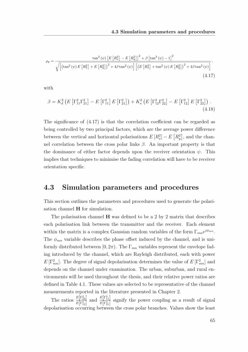
4.3 Simulation parameters and procedures
ρp =tan2 (ψ)
[E[R2
x
]− E
[R2y
]]2+ β
[tan2 (ψ)− 1
]2√[(tan2 (ψ)E
[R2x
]+ E
[R2
y
])2+ 4β tan2 (ψ)
] [(E[R2
x
]+ tan2 (ψ)E
[R2
y
])2+ 4β tan2 (ψ)
] ,(4.17)
with
β = K2d
(E[Γ211Γ
221
]− E
[Γ211
]E[Γ221
])+K2
s
(E[Γ212Γ
222
]− E
[Γ212
]E[Γ222
]).
(4.18)
The significance of (4.17) is that the correlation coefficient can be regarded as
being controlled by two principal factors, which are the average power difference
between the vertical and horizontal polarisations E [R2x]−E
[R2
y
], and the chan-
nel correlation between the cross polar links β. An important property is that
the dominance of either factor depends upon the receiver orientation ψ. This
implies that techniques to minimise the fading correlation will have to be receiver
orientation specific.
4.3 Simulation parameters and procedures
This section outlines the parameters and procedures used to generate the polari-
sation channel H for simulation.
The polarisation channel H was defined to be a 2 by 2 matrix that describes
each polarisation link between the transmitter and the receiver. Each element
within the matrix is a complex Gaussian random variables of the form Γmnejϕmn .
The ϕmn variable describes the phase offset induced by the channel, and is uni-
formly distributed between [0, 2π). The Γmn variables represent the envelope fad-
ing introduced by the channel, which are Rayleigh distributed, each with power
E [Γ2mn]. The degree of signal depolarisation determines the value of E [Γ2
mn] and
depends on the channel under examination. The urban, suburban, and rural en-
vironments will be used throughout the thesis, and their relative power ratios are
defined in Table 4.1. These values are selected to be representative of the channel
measurements reported in the literature presented in Chapter 2.
The ratiosE[Γ2
22]E[Γ2
12]and
E[Γ211]
E[Γ221]
signify the power coupling as a result of signal
depolarisation occurring between the cross polar branches. Values show the least
65

CHAPTER 4. Model of the Generalised Polarisation DiversitySystem
Urban Suburban Rural
E[Γ222]
E[Γ212]
6 dB 10 dB 12 dB
E[Γ211]
E[Γ221]
6 dB 10 dB 12 dB
E[Γ222]
E[Γ211]
3 dB 2 dB 0 dB
Table 4.1: Polarisation channel relative power ratios.
discrepancy in the urban environments as this channel is obstacle rich and best
facilitates the transfer of power between the vertical and horizontal polarisations.
The ratioE[Γ2
22]E[Γ2
11]represent the relative power difference between the vertical
and horizontal polarisations. This ratio is used to describe the asymmetric at-
tenuation between the vertical and horizontal polarisations. Electric field vectors
that are parallel to channel obstacles suffer less attenuation than those that are
orthogonal to channel obstacles [44]. In the urban environment where buildings
are upright and constitute the majority of the channel obstacles, the vertical
polarisation is expected to experience less attenuation than the horizontal polar-
isation. On the other hand, open nature of the rural environment promotes an
equal attenuation between the vertical and horizontal polarisations.
In all three environments, derivations of the envelope fading between the cross
polar links Γ11 and Γ21, and Γ22 and Γ12 have been assumed correlated to maintain
generality. In simulation, however, both correlated and uncorrelated channels will
be examined in subsequent chapters. The channel correlation assumed in each
simulation will be explicitly stated. If the channel is assumed to be correlated,
the correlation coefficient between Γ11 and Γ21; and Γ22 and Γ12 have been set
to 0.4. This is reflective of worst case scenario, since the channel correlation
coefficients, as summarised in Chapter 2 are generally closer to 0. Correlated
Rayleigh channels were generated using the algorithm presented in [30].
4.4 Summary
A generalised model of a polarisation diversity system which accounts for trans-
mitter and receiver orientations, as well as the type of polarisation of the transmit-
ted signal is established. At the transmitter, a pair of linearly polarised elements
66

4.4 Summary
mounted in an orthogonal manner with orientation α is assumed. This antenna
structure generally produces signals that are elliptically polarised, but can be
easily modified to create linearly or circularly polarised signals. The polarisation
channel is established as a 2 by 2 matrix that describes the interactions between
the vertical and horizontal polarisations. At the receiver side, two linearly po-
larised elements mounted in an orthogonal manner with orientation ψ is used to
capture diversity signals.
Generalised expressions for the branch power ratio and correlation coefficient
derived from his model serves as the basis for subsequent chapters. The param-
eters and procedures for the simulation of such diversity systems have also been
presented.
67


Chapter 5
Polarisation Diversity using
Linear Polarisation
The polarisation diversity receiver is traditionally implemented with two linearly
polarised antenna elements aligned vertically and horizontally to capture the ver-
tical and horizontal polarisations. [35,55,95]. Signals emitted from the transmitter
are typically vertically polarised signals. Diversity signals captured in this con-
figuration exhibit low fading correlation, but have an undesirable large average
power imbalance.
Resolving this power imbalance problem between the vertical and horizon-
tal polarisations can be achieved with the realignment of the receiver diversity
antennas at angles ±ψ relative to the vertical axis [28, 48]. The established an-
tenna symmetry reduces the average power difference, but is at the expense of
an increased fading correlation.
While the symmetric antenna structure is easily achievable at the base station,
the geometry is difficult to maintain for the mobile station. This is because
mobile units are hand held devices and can have variable orientations. The power
imbalance problem re-emerges when geometric symmetry of the antennas are
disturbed through changes in the antenna orientation.
The primary objective of this chapter is to quantify diversity parameters of
traditional polarisation diversity systems after antenna orientations at both the
transmitter and receiver terminals are taken into account. A key limitation in
this implementation of polarisation diversity is demonstrated, showing that diver-
sity parameters can easily exceed acceptable parameter bounds with a change in
antenna orientations. The work presented in this chapter uses the mathematical

CHAPTER 5. Polarisation Diversity using Linear Polarisation
y
x
V1α
Transmitter
H11
H22
H12
H21
Hpol
Vpol
Hpol
Vpol
Channel Receiver
y
x
R2
R1
Figure 5.1: The traditional polarisation diversity in the mobile uplink.
framework established previously in Chapter 4.
5.1 Traditional polarisation diversity
The traditional polarisation diversity scheme is implemented in the uplink and
utilises two linearly polarised antennas at the base station mounted orthogonally
to capture signals residing in the vertical and horizontal polarisations. In relation
to the generalised polarisation diversity model, this is equivalent to having the
receiver orientation is fixed at ψ = 0◦.
At the mobile transmitter, the emitted signal is usually assumed to be princi-
pally vertically polarised. This is achieved with the assignment of values A1 = A,
A2 = 0 and θ = 0 to the generalised polarisation diversity model. With such an
assignment, V1 will be the only transmitting antenna emitting a linearly polarised
signal. However, since the mobile unit is a hand held device, its orientation α
should be regarded as a variable, and free to rotate in the xy plane. Fig. 5.1
illustrates a diagram of this polarisation diversity system.
Using the generalised expressions of the BPR (4.10) and correlation coefficient
(4.17), the respective diversity parameters are calculated as,
BPR =tan2 (α)E [Γ2
21] + E [Γ222]
tan2 (α)E [Γ211] + E [Γ2
12], (5.1)
ρp =sin4 (α) (E [Γ2
11Γ221]− E [Γ2
11]E [Γ221]) + cos4 (α) (E [Γ2
12Γ222]− E [Γ2
12]E [Γ222])(
sin2 (α)E [Γ211] + cos2 (α)E [Γ2
12]) (
sin2 (α)E [Γ221] + cos2 (α)E [Γ2
22]) .
(5.2)
70
5.1 Traditional polarisation diversity
The correlation coefficient, as discussed previously in Chapter 4, can be re-
garded as an expression influenced by the power difference between the horizontal
and vertical polarisations, and the channel correlation between the cross polar
links. In the traditional polarisation diversity scheme where the alignment of the
receiver antennas are along the vertical and horizontal axes with ψ = 0◦, the
generalised expression of ρp simplifies into (5.2), a form that is influenced only
by the channel correlation between the cross polar links. Historical developments
assuming a fixed vertically polarised transmitter with α = 0◦ further implies that
the correlation coefficient becomes entirely dependent on the covariance between
Γ222 and Γ2
12. Since empirical measurements in the literature as seen in Chapter 2
indicate at worst a very weak fading correlation between these links, histori-
cal treatments have used this to justify the assumptions of uncorrelated fading
between vertical and horizontal polarisations. The implications of such an as-
sumption is significant, because the covariance between R21 and R2
2 would always
zero and therefore not allow the influence of antenna orientations to be properly
studied. Examination of the fading correlation coefficient as a function of antenna
orientations necessarily requires a generalised treatment with correlated channel
links.
For the BPR, (5.1) the significant feature here is that it is clearly influenced
by the transmitter orientation α. This means that the average branch power
of diversity branches will generally be in an unbalanced state for any arbitrary
orientation. Nevertheless, channel specific transmitter orientations that allows for
average power balance between the vertical and horizontal polarisation diversity
branches do exist and can be determined.
71

CHAPTER 5. Polarisation Diversity using Linear Polarisation
5.1.1 Transmitter orientation for power balanced diver-
sity branches
The ideal transmitter orientation for an optimal BPR is calculated from (5.1), by
setting the BPR to equal 0 dB and then solving for α
BPR = 1 =tan2 (α)E [Γ2
21] + E [Γ222]
tan2 (α)E [Γ211] + E [Γ2
12](5.3)
⇒ tan2 (α)E[Γ211
]+ E
[Γ212
]= tan2 (α)E
[Γ221
]+ E
[Γ222
](5.4)
⇒ tan2 (α) =E [Γ2
22]− E [Γ212]
E [Γ211]− E [Γ2
21](5.5)
⇒αopt = arctan
(√E [Γ2
22]− E [Γ212]
E [Γ211]− E [Γ2
21]
). (5.6)
For the previously defined urban, suburban and rural environments, these opti-
mum transmitter orientation are calculated to be 54.73◦, 51.54◦ and 45◦ respec-
tively. These results have been summarised in Table 5.1.
Urban Suburban Rural
αopt 54.73◦ 51.54◦ 45◦
Table 5.1: Transmitter orientations for power balanced BPR.
The achieved average power balance between R1 and R2 however, is only
temporary and can be lost following a variation in α. This can be demonstrated
by calculating the gradient of the BPR as a function of the transmitter orientation,
dBPR
dα=
2 tan (α) sec2 (α) (E [Γ221]E [Γ2
12]− E [Γ222]E [Γ2
11])
(tan2 (α)E [Γ211] + E [Γ2
12])2 . (5.7)
At the ideal transmitter orientation α = αopt, the gradient of the BPR is gen-
erally non zero. In particular, the rate of change evaluated in linear scale are
−2.546, −3.3597 and −3.5252 for the urban, suburban and rural environments
respectively. This demonstrates that power balance can easily be lost following a
change in the transmitter orientation.
72

5.1 Traditional polarisation diversity
0 10 20 30 40 50 60 70 80 90−15
−10
−5
0
5
10
15
Transmitter Orientation α (degrees)
BP
R (
dB)
Urban SimulatedUrban TheoreticalSuburban SimulatedSuburban TheoreticalRural SimulatedRural Theoretical
54.73°
Optimal BPR
51.54°
45°
Figure 5.2: BPR simulation for the traditional polarisation diversity as a functionof the transmitter orientation in different environments. Optimum transmitterorientations for power balanced BPR are marked by the dotted lines.
5.1.2 Performance of traditional polarisation diversity
The performance of the traditional polarisation diversity is demonstrated through
computer simulations of the average BPR and fading correlation coefficient.
In Fig. 5.2, the average BPR in the urban, suburban and rural environments
are plotted as a function of the transmitter orientation α. The angles at which
the power balanced BPR are achieved have also been marked. It can be seen that
small change in the transmitter orientation causes power balance to be lost. In
the urban environment, a ±10◦ variation away from αopt causes a corresponding
shift in the BPR by approximately ±2 dB. The loss of power balance is even more
severe in the suburban and rural environments, where a ±10◦ variation away from
αopt causes the BPR to shift by ±2.5 dB and ±3 dB respectively.
Simulated results for the fading correlation coefficient between antennas R1
and R2 in the urban, suburban and rural environments as a function of the
transmitter orientation α are presented in Fig. 5.3. Simulation were performed
with the assumption of correlated channels, with a channel correlation coefficient
set to 0.4. The results show that the fading correlation coefficient is at a minimum
when the transmitter orientation is operating at αopt.
73

CHAPTER 5. Polarisation Diversity using Linear Polarisation
0 10 20 30 40 50 60 70 80 900
0.05
0.1
0.15
0.2
0.25
0.3
0.35
0.4
0.45
Transmitter Orientation α (degrees)
Cor
rela
tion
Coe
ffici
ent ρ
Urban SimulatedUrban TheoreticalSuburban SimulatedSuburban TheoreticalRural SimulatedRural Theoretical0.128
0.0670.045
54.73°
51.54°45°
Figure 5.3: Correlation coefficient simulation for the traditional polarisation di-versity as a function of the transmitter orientation in different environments. Thecorrelation coefficient values at αopt are marked by the dotted lines.
The combined result of the BPR and correlation coefficient demonstrates that
the traditional polarisation diversity with the transmitter orientation set to αopt,
allows for a balanced BPR and very low fading correlation, conditions that are
favourable for diversity action. One disadvantage is the required knowledge of
the channel statistics in order to calculate this optimum angle. The other more
severe disadvantage is that the transmitter orientation must remain fixed, and
a small change in the antenna geometry causes power balance to be lost. Such
constraints mean that the traditional polarisation diversity scheme is not suitable
for the mobile uplink.
5.2 Symmetric polarisation diversity
One of the most successful methods to address the power imbalance problem is to
use a receiver antenna geometry that is symmetric about the vertical y axis [48].
In this section, antenna rotations are introduced at the receiver side to examine
its effects on the diversity parameters. The receiver orientation of ψ = 45◦ is of
particular interest because the antenna elements are symmetric with respect to
the y axis.
74

5.2 Symmetric polarisation diversity
5.2.1 Modifying the receiver orientation for power bal-
ance
The investigation begins with the assumption of a linearly polarised transmit-
ter with an arbitrary orientation. The generalised expression of the BPR, as a
function of the XPD, is
BPR =tan2 (ψ) + XPD
1 + XPD tan2 (ψ). (5.8)
The receiver antenna orientation that allows for branch power balance is calcu-
lated by setting BPR to 0 dB and solving for the value of ψ
BPR = 1 =tan2 (ψ) + XPD
1 + XPD tan2 (ψ)(5.9)
1 + XPD tan2 (ψ) = tan2 (ψ) + XPD (5.10)
tan2 (ψ) =XPD− 1
XPD− 1= 1 (5.11)
⇒ ψ =45◦ . (5.12)
This calculation shows that the optimum receiver antenna orientation for a power
balanced BPR is at ψ = 45◦. Importantly, this reflects the case of a geometrically
symmetric antenna configuration with R1 and R2 aligned at angles ±45◦ with
respect to the y axis.
With this configuration, the branch power imbalance problems are resolved.
However, of greater significance is the implications this has on the transmitter
orientations. From the generalised expression of the BPR (4.10), effects of the
transmitter orientations are confined within the XPD term. If power balance is
achieved when ψ = 45◦ irrespective of the XPD, it also means that power balance
is achieved irrespective of the transmitter orientation α. Such a result demon-
strates that power imbalance problems originally induced by variable transmitter
orientations are also resolved.
The symmetric antenna geometry implemented at the diversity receiver is ex-
tremely effective at ensuring a power balanced BPR. However, a full description
of diversity performance also requires the examination into the fading correla-
tion coefficient. Analysis begins at the generalised correlation coefficient (4.17)
rewritten here again as,
75
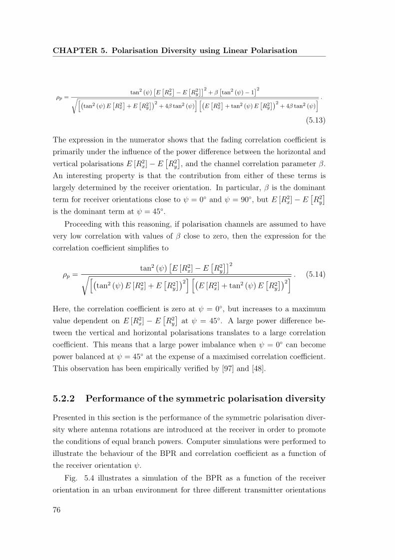
CHAPTER 5. Polarisation Diversity using Linear Polarisation
ρp =tan2 (ψ)
[E[R2
x
]− E
[R2y
]]2+ β
[tan2 (ψ)− 1
]2√[(tan2 (ψ)E
[R2
x
]+ E
[R2y
])2+ 4β tan2 (ψ)
] [(E[R2
x
]+ tan2 (ψ)E
[R2
y
])2+ 4β tan2 (ψ)
] .(5.13)
The expression in the numerator shows that the fading correlation coefficient is
primarily under the influence of the power difference between the horizontal and
vertical polarisations E [R2x]− E
[R2
y
], and the channel correlation parameter β.
An interesting property is that the contribution from either of these terms is
largely determined by the receiver orientation. In particular, β is the dominant
term for receiver orientations close to ψ = 0◦ and ψ = 90◦, but E [R2x] − E
[R2
y
]is the dominant term at ψ = 45◦.
Proceeding with this reasoning, if polarisation channels are assumed to have
very low correlation with values of β close to zero, then the expression for the
correlation coefficient simplifies to
ρp =tan2 (ψ)
[E [R2
x]− E[R2
y
]]2√[(tan2 (ψ)E [R2
x] + E[R2
y
])2] [(E [R2
x] + tan2 (ψ)E[R2
y
])2] . (5.14)
Here, the correlation coefficient is zero at ψ = 0◦, but increases to a maximum
value dependent on E [R2x] − E
[R2
y
]at ψ = 45◦. A large power difference be-
tween the vertical and horizontal polarisations translates to a large correlation
coefficient. This means that a large power imbalance when ψ = 0◦ can become
power balanced at ψ = 45◦ at the expense of a maximised correlation coefficient.
This observation has been empirically verified by [97] and [48].
5.2.2 Performance of the symmetric polarisation diversity
Presented in this section is the performance of the symmetric polarisation diver-
sity where antenna rotations are introduced at the receiver in order to promote
the conditions of equal branch powers. Computer simulations were performed to
illustrate the behaviour of the BPR and correlation coefficient as a function of
the receiver orientation ψ.
Fig. 5.4 illustrates a simulation of the BPR as a function of the receiver
orientation in an urban environment for three different transmitter orientations
76
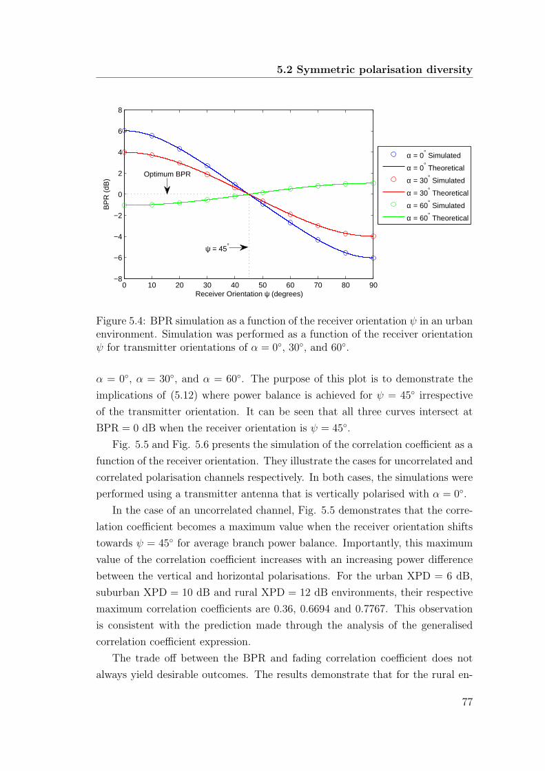
5.2 Symmetric polarisation diversity
0 10 20 30 40 50 60 70 80 90−8
−6
−4
−2
0
2
4
6
8
Receiver Orientation ψ (degrees)
BP
R (
dB)
α = 0° Simulated
α = 0° Theoretical
α = 30° Simulated
α = 30° Theoretical
α = 60° Simulated
α = 60° Theoretical
Optimum BPR
ψ = 45°
Figure 5.4: BPR simulation as a function of the receiver orientation ψ in an urbanenvironment. Simulation was performed as a function of the receiver orientationψ for transmitter orientations of α = 0◦, 30◦, and 60◦.
α = 0◦, α = 30◦, and α = 60◦. The purpose of this plot is to demonstrate the
implications of (5.12) where power balance is achieved for ψ = 45◦ irrespective
of the transmitter orientation. It can be seen that all three curves intersect at
BPR = 0 dB when the receiver orientation is ψ = 45◦.
Fig. 5.5 and Fig. 5.6 presents the simulation of the correlation coefficient as a
function of the receiver orientation. They illustrate the cases for uncorrelated and
correlated polarisation channels respectively. In both cases, the simulations were
performed using a transmitter antenna that is vertically polarised with α = 0◦.
In the case of an uncorrelated channel, Fig. 5.5 demonstrates that the corre-
lation coefficient becomes a maximum value when the receiver orientation shifts
towards ψ = 45◦ for average branch power balance. Importantly, this maximum
value of the correlation coefficient increases with an increasing power difference
between the vertical and horizontal polarisations. For the urban XPD = 6 dB,
suburban XPD = 10 dB and rural XPD = 12 dB environments, their respective
maximum correlation coefficients are 0.36, 0.6694 and 0.7767. This observation
is consistent with the prediction made through the analysis of the generalised
correlation coefficient expression.
The trade off between the BPR and fading correlation coefficient does not
always yield desirable outcomes. The results demonstrate that for the rural en-
77

CHAPTER 5. Polarisation Diversity using Linear Polarisation
0 10 20 30 40 50 60 70 80 900
0.1
0.2
0.3
0.4
0.5
0.6
0.7
0.8
0.9
1
Receiver Orientation ψ (degrees)
Cor
rela
tion
Coe
ffici
ent ρ
Urban SimulatedUrban TheoreticalSuburban SimulatedSuburban TheoreticalRural SimulatedRural Theoretical
ρ = 0.6694ρ = 0.36
ρ = 0.7767
Figure 5.5: Correlation coefficient as a function of the receiver orientation ψ inuncorrelated channels.
0 10 20 30 40 50 60 70 80 900
0.1
0.2
0.3
0.4
0.5
0.6
0.7
0.8
0.9
1
Receiver Orientation ψ (degrees)
Cor
rela
tion
Coe
ffici
ent ρ
Urban SimulatedUrban TheoreticalSuburban SimulatedSuburban TheoreticalRural SimulatedRural Theoretical
ρ = 0.713
ρ = 0.2866
ρ = 0.5912
Figure 5.6: Correlation coefficient as a function of the receiver orientation ψ incorrelated channels.
78

5.3 Summary
vironment, a 12 dB XPD translates to a maximum correlation coefficient greater
than the 0.7 threshold for effective diversity. Even for the suburban environment,
the fading correlation coefficient of 0.6694 is regarded to be very high.
Fig. 5.6 illustrates the behaviour of the fading correlation coefficient in corre-
lated polarisation channels as a function of the receiver orientation. The fading
correlation coefficient now takes a higher value of 0.4 at the orientations ψ = 0◦
and ψ = 90◦. This is to be expected since the channel correlation parameter β
is the dominant term affecting fading correlation at these two orientations. Sim-
ilarly, the contribution of β diminishes when the orientation is at ψ = 45◦, and
it is the power difference between the vertical and horizontal polarisations that
becomes dominant.
For the rural and suburban environments, the variation of the receiver ori-
entation from ψ = 0◦ to ψ = 45◦ causes the fading correlation to increase to a
maximum value. The large power imbalance between the vertical and horizontal
polarisations is responsible for the large fading correlation at ψ = 45◦.
The results for the urban environment may appear unusual, with the value
of the fading correlation coefficient reducing to a minimum at ψ = 45◦. Such
an outcome is reasonable and explainable by once again analysing the relative
contributions from the terms E [R2x]−E
[R2
y
]and β in the numerator of (5.13). A
fading correlation coefficient of 0.4 at ψ = 0◦ is primarily due to the parameter β.
The term E [R2x]−E
[R2
y
]does not contribute to the correlation coefficient at this
receiver orientation. At ψ = 45◦, however, the contribution from β diminishes
and it is E [R2x] − E
[R2
y
]that becomes the dominant term, yielding a fading
correlation coefficient of 0.2886. The reason why this value is a minimum rather
than a maximum is simply because the effects of β at ψ = 0◦ gives a greater
fading correlation than the effects of E [R2x] − E
[R2
y
]at ψ = 45◦. In fact, if
the XPD were equal to 0 dB making E [R2x] = E
[R2
y
], the value of the fading
correlation coefficient will not only minimum, but also ideal at zero.
5.3 Summary
Traditional polarisation diversity is implemented at the base station receiver of
the mobile uplink, and uses two linearly polarised antenna elements at the base
station to capture diversity signals in the vertical and horizontal polarisations.
Studies have historically assumed the mobile station to be in a fixed orientation
79
CHAPTER 5. Polarisation Diversity using Linear Polarisation
emitting only a principally vertically polarised signal. Such a constraint is unreal-
istic since mobile units are hand held devices and can take arbitrary orientations.
This research demonstrates that both the BPR and correlation coefficient for
the traditional polarisation diversity scheme are variable as a function of the
transmitter orientation. Variations of the BPR within the suburban and rural
environments are particularly severe, with values as high as 10 dB and 12 dB
respectively. Despite these large variations, the second order statistics of the po-
larisation channel can be used to calculate an optimum transmitter orientation
αopt, at which a power balanced BPR and minimised correlation coefficient are
maintained. This method to achieve power balanced diversity branches, how-
ever, is easily influenced by changes in the transmitter orientation. This research
demonstrates that a small ±10◦ rotation away from αopt can increase the BPR
by 2 to 3 dB. The arbitrary and variable nature of the transmitter orientation in
the uplink means this solution for a power balanced BPR is infeasible.
The better method to achieve a power balanced BPR is to rotate the tradi-
tional polarisation diversity receiver and realign the antenna elements at angles
±45◦ relative to the vertical axis. Such an implementation converts an otherwise
large XPD into a power balanced BPR. In fact, the equations show that both
diversity antennas will remain power balanced irrespective of the XPD. Most sig-
nificantly, this implies that the BPR remains power balanced irrespective of the
transmitter orientation, as the transmitter orientation variable α is embedded in
the XPD term. An increase in the XPD due to a variation in α has no influence
on the BPR.
The principal disadvantage of this symmetric polarisation diversity scheme
is that the achieved power balanced BPR is at the cost of an increased fading
correlation coefficient. In a typical uncorrelated polarisation channel, a large XPD
was shown to convert into a large fading correlation coefficient. For example, in
the rural environment, a XPD of 12 dB was converted into a BPR of 0 dB, at
the expense of a maximised fading correlation coefficient with a value of 0.7767,
above the acceptable threshold of 0.7.
The generalised expression for the fading correlation coefficient describes this
trade-off behaviour, and demonstrates the interaction between the polarisation
channel correlation parameter β and power difference between vertical and hor-
izontal polarisations E [R2x] − E
[R2
y
]. Significantly, it is the receiver orientation
which determines the how each of these terms contribute to the overall fading
80

5.3 Summary
correlation coefficient. In the case of the symmetric polarisation diversity scheme
where ψ = 45◦, the fading correlation coefficient is entirely influenced by the
power difference between the vertical and horizontal polarisations. The implica-
tion of this result is that excessive increases of the fading correlation coefficient
can be suppressed if the XPD is controlled.
Chapters 6 and 7 of this thesis demonstrates effective techniques to control
the XPD and optimise the operating conditions for polarisation diversity.
81


Chapter 6
Reducing Excess Correlation
With Circular Polarisation
The previous chapter investigated the influence of variable transmitter and re-
ceiver antenna orientations on the traditional polarisation diversity scheme. Di-
versity parameters were demonstrated to be suboptimal, and highly sensitive to
changes in the antenna orientation at both ends of the communications link. Us-
ing a symmetric receiver antenna geometry with ψ = 45◦ successfully achieves
a power balanced BPR irrespective of the transmitter orientation, but is at the
expense of an increased the correlation coefficient.
Two factors influencing the fading correlation coefficient are the power differ-
ence between the vertical and horizontal polarisations E [R2x] − E
[R2
y
], and the
channel correlation parameter β. When the receiver antenna orientation is fixed
at ψ = 45◦, the fading correlation coefficient is primarily determined by the power
difference between the vertical and horizontal polarisations. This means that if
the XPD can be controlled, a power balanced BPR can be achieved without an
excessive increase in the fading correlation coefficient.
The primary objective of this chapter is to resolve the problem of an excess
increase in the fading correlation coefficient when the receiver antenna orienta-
tion is set to ψ = 45◦. The solution proposed in this chapter is to address the
problem from the transmitter side by emitting signals that are less dependent on
the channel for power coupling. A circularly polarised signal is one such example
suitable for this task because the electric field vector has a constant magnitude
that changes direction in a rotary manner in the plane orthogonal to the direc-
tion of propagation. This means that the power of transmitted signal becomes

CHAPTER 6. Reducing Excess Correlation With CircularPolarisation
uniformly distributed in all polarisations and facilitates the conditions for power
coupling, potentially reducing the XPD. A further advantage of circular polarisa-
tion is that the generated signals are invariant to the transmitter orientation. The
direction of the electric field vector is preserved irrespective of the transmitter
orientation or its antenna alignment.
The inspiration of using circularly polarised signals comes from its application
in satellite tracking and communications. Generally, signals can have its polarisa-
tion states changed as it passes through the Earth’s ionosphere. This means that
even if antennas on the Earth station were matched with the orientation of the
satellite there is no guarantee that the polarisation of the received signal matches
with the polarisation of the satellite antenna. Circularly polarised signals pro-
vides greater robustness against polarisation shifts as there is a component of the
electric field in all directions orthogonal to the direction of propagation. Even if
changes in the polarisation states were induced, at least some of the signal will
still be recoverable.
The novelty of this chapter is using circularly polarised signals as a transmitter
orientation invariant method to curtail the XPD and in turn maintain the fading
correlation coefficient below the 0.7 threshold required for effective diversity.
6.1 System model and diversity parameters
In relation to the model of the generalised diversity system modelled in Chapter 4,
the transmission of a circularly polarised signal is achieved with the assignment
of A1 = A, A2 = A and θ = π/2. Both the V1 and V2 antennas are in transmission
and have equal amplitudes, but are out of phase by π/2 radians. A circularly
polarised signal is generated because the tip of the resultant electric field vector
traces out a circle as a function of time.
6.1.1 Mobile uplink
The behaviour of the XPD as a result of using circular polarisation is investigated
in the mobile uplink by assigning an orientation of ψ = 0◦ to the base station
receiver. Such setup aligns the R1 and R2 antenna elements along the vertical
and horizontal axes, with a calculated BPR equal to the XPD. This allows the
XPD, being the variable of interest, to be directly observed.
84

6.1 System model and diversity parameters
y
x
V1
V2
α
Transmitter
H11
H22
H12
H21
Hpol
Vpol
Hpol
Vpol
Channel Receiver
y
x
R1
R2
Figure 6.1: Polarisation diversity using circular polarisation with variable trans-mitter orientation in the mobile uplink.
The mobile station is acting as the transmitter terminal, and its orientation
α is assumed to be variable. The model of the described mobile uplink with
the mobile terminal configured to transmit in a circularly polarised manner is
illustrated in Fig. 6.1.
The diversity parameters, BPR and fading correlation coefficient are calcu-
lated using the generalised expressions of (4.10) and (4.17) as,
BPR = XPD =E [Γ2
21] + E [Γ222]
E [Γ211] + E [Γ2
12]. (6.1)
ρp =E [Γ2
11Γ221]− E [Γ2
11]E [Γ221] + E [Γ2
12Γ222]− E [Γ2
12]E [Γ222]
(E [Γ221] + E [Γ2
22]) (E [Γ212] + E [Γ2
11]), (6.2)
These expressions demonstrate three important features of transmitting a circu-
larly polarised signal. Firstly, both expressions are independent of the transmitter
orientation α and demonstrates that the transmitter orientation invariant prop-
erty has been retained and achieved from the transmitter side.
Secondly, expression of (6.1) shows that the XPD is dependent entirely on
the second order channel statistics. The corresponding XPD values for each the
urban, suburban and rural environments have been calculated using the relative
power ratios defined in Table 4.1 to be 1.761 dB, 1.627 dB and 0 dB respec-
tively. This shows that even if power coupling between the polarisation channels
is low and promotes for a large XPD in linearly polarisation, circularly polarised
transmission can significantly reduce the XPD. These calculated XPD values are
summarised in Table 6.1.
85

CHAPTER 6. Reducing Excess Correlation With CircularPolarisation
y
x
V1
V2
Transmitter
H11
H22
H12
H21
Hpol
Vpol
Hpol
Vpol
Channel Receiver
y
x
ψ R1
R2
Figure 6.2: Polarisation diversity using circular polarisation with variable receiverorientation in the mobile downlink.
Urban Suburban Rural
XPD 1.761 dB 1.627 dB 0 dB
Table 6.1: XPD obtained in each environment under circular polarisation
Thirdly, the numerator of the fading correlation coefficient demonstrates that
it is entirely dependent upon the covariance between Γ211 and Γ2
21; and Γ212 and
Γ222. The review of experimental results in Chapter 2 shows that the polarisation
channel exhibits very low channel correlation, which means these covariance terms
are expected to be small, resulting in a small fading correlation coefficient.
6.1.2 Mobile downlink
Transmission using circularly polarised signals have been demonstrated to effec-
tively suppress high levels of the XPD. This would mean that excessive increases
in fading correlation coefficient should not occur if receiver antennas were re-
aligned to ψ = 45◦ for a power balanced BPR.
Investigation into the behaviour of the BPR and fading correlation coefficient
will continue in the mobile downlink, where the diversity parameters are examined
in the presence of a variable receiver orientation. The base station terminal has
been assumed to be transmitting circular polarisation from a fixed orientation
at α = 0◦. This transmitter orientation was chosen to simplify analysis, though
its choice can be completely arbitrary and does not influence the outcome of
the result. The diagram illustrating the antenna configurations of the mobile
downlink is presented in Fig. 6.2.
86

6.1 System model and diversity parameters
The expression for the BPR as calculated from the generalised BPR expression
(4.10) is
BPR =(E [Γ2
11] + E [Γ212]) tan
2 (ψ) + E [Γ221] + E [Γ2
22]
E [Γ211] + E [Γ2
12] + tan2 (ψ) (E [Γ221] + E [Γ2
22]). (6.3)
Similarly, the correlation coefficient as calculated from the generalised corre-
lation coefficient expression (4.17), is
ρp =tan2 (ψ)
(E[R2x
]− E
[R2y
])2+ 4β
[tan2 (ψ)− 1
]2√[(tan2 (ψ)E
[R2x
]+ E
[R2
y
])2+ 4β tan2 (ψ)
] [(E[R2
x
]+ tan2 (ψ)E
[R2
y
])2+ 4β tan2 (ψ)
] ,(6.4)
with
E[R2
y
]=A2
(E[Γ221
]+ E
[Γ222
])(6.5)
E[R2
x
]=A2
(E[Γ211
]+ E
[Γ212
]), (6.6)
β = A4(E[Γ211Γ
221
]− E
[Γ211
]E[Γ221
]+ E
[Γ212Γ
222
]− E
[Γ212
]E[Γ222
]). (6.7)
In particular, when the receiver orientation is symmetric about the y axis at
ψ = 45◦, the BPR becomes power balanced, with
BPR =E [Γ2
11] + E [Γ212] + E [Γ2
21] + E [Γ222]
E [Γ211] + E [Γ2
12] + E [Γ221] + E [Γ2
22](6.8)
=0 dB . (6.9)
This is consistent with the results of the previous chapter, where a power balanced
BPR is achieved irrespective of the XPD.
For the fading correlation coefficient, the assignment of ψ = 45◦ simplifies
(6.4) to
ρp =
(E [R2
x]− E[R2
y
])2(E [R2
x] + E[R2
y
])2+ 4β
. (6.10)
This result is once again consistent with the observations in the last chapter,
where a symmetric receiver antenna configuration with ψ = 45◦ causes the fading
87

CHAPTER 6. Reducing Excess Correlation With CircularPolarisation
correlation coefficient to be primarily influenced by the power difference between
the vertical and horizontal polarisations. Values of the XPD in circular polari-
sation previously calculated and summarised in Table 6.1 show a small relative
difference between the vertical and horizontal polarisations, implying that the
fading correlation coefficient will not significantly inflate.
A more significant observation, however, is that the fading correlation coeffi-
cient also becomes transmitter orientation invariant. The terms E [R2x], E
[R2
y
]and β as expressed in (6.5), (6.6) and (6.7), are all independent of α.
6.2 Results
Computer simulations were performed to validate the theoretical developments
of the diversity parameters when circularly polarised signals are used for trans-
mission. The mobile uplink and downlink scenarios established in the previous
section were simulated separately and follows the procedure established in Chap-
ter 4.
6.2.1 Mobile uplink
In the scenario of the mobile uplink, the primary objective is to examine the
behaviour of the XPD when circularly polarised signals are transmitted. The
deliberate alignment of receiver antennas along the vertical and horizontal axes
with ψ = 0◦ means the examined BPR is equivalent to the XPD. The simulation
of the BPR as a function of the transmitter orientation is presented in Fig. 6.3.
This result demonstrates two important features. First, the level of power
imbalance between the vertical and horizontal polarisations have significantly re-
duced. For example, in the urban environment, circular polarisation yielded a
maximum XPD of 1.761 dB, where as traditional polarisation diversity using lin-
ear polarisation as illustrated in Fig. 5.2 could be as high as 6 dB. The fact
that the urban channel gave higher values of power imbalance than the suburban
and rural channels, despite being the environment that facilitates the best condi-
tions for power coupling suggests that the observed power difference is the direct
consequence of the asymmetric attenuation between the vertical and horizontal
polarisations.
The second feature of the result is that the XPD remains constant as a function
of the α, and therefore confirms the orientation invariant properties from the
88

6.2 Results
0 10 20 30 40 50 60 70 80 90−1
−0.5
0
0.5
1
1.5
2
2.5
3
Transmitter Orientation α (degrees)
BP
R=
XP
D (
dB)
Urban SimulatedUrban TheoreticalSuburban SimulatedSuburban TheoreticalRural SimulatedRural Theoretical
XPD = 1.761dB
XPD = 0dB
XPD = 1.627dB
Figure 6.3: BPR simulation for the mobile uplink with circular polarisation asa function of the transmitter orientation in different environments. With ψ =0◦, the BPR is equivalent to the XPD. The constant XPD demonstrates theorientation invariant properties of circular polarisation.
transmitter side when circularly polarised signals are used.
Simulation results for the fading correlation coefficient are presented in Fig.
6.4. As expected, following the examination of equation (6.10) in the previous
section, the fading correlation coefficient is also invariant to changes in the trans-
mitter orientation. Comparing the values of the fading correlation coefficient here
against the traditional polarisation diversity with linear polarisation in Fig. 5.3,
shows that circularly polarised transmission is generally at an advantage with
significantly lower values across the majority of orientations. However, linear
polarisation does have slightly lower correlation when α = αopt.
6.2.2 Mobile downlink
In the scenario for the mobile downlink, both the BPR and fading correlation
coefficient are simulated as a function of the receiver orientation. The behaviour
of both diversity parameters at the receiver orientation of ψ = 45◦ is of particular
interest, as the rationale for using circular polarisation was to address the problem
of an excessive increase in fading correlation.
The transmitter orientation was assumed fixed at α = 0◦, however with cir-
89

CHAPTER 6. Reducing Excess Correlation With CircularPolarisation
0 10 20 30 40 50 60 70 80 900
0.02
0.04
0.06
0.08
0.1
0.12
0.14
0.16
0.18
0.2
Transmitter Orientation α (degrees)
Cor
rela
tion
Coe
ffici
ent ρ
Urban SimulatedUrban TheoreticalSuburban SimulatedSuburban TheoreticalRural SimulatedRural Theoretical
ρ = 0.1481
ρ = 0.04466
ρ = 0.07197
Figure 6.4: Correlation coefficient simulation for the mobile uplink with circularpolarisation as a function of the transmitter orientation in different environments.The correlation coefficient is also transmitter orientation invariant.
cular polarisation, this assignment can be arbitrary and yields identical results.
Presented in Fig. 6.5 is the simulated BPR as a function of the receiver
orientation. The results illustrated here are consistent with the characteristics
derived from the theoretical treatment in the previous section and demonstrates
branch power balance when the receiver orientation is set to ψ = 45◦. The power
balance is guaranteed, irrespective of the environment and its XPD.
A second significant feature of the BPR is that the values obtained are better
than linear polarisation. In particular, taking the urban environment result, and
comparing this with Fig. 5.4, a potential ±6 dB variation in the BPR is reduced
to ±1.774 dB.
Results for the correlation coefficient simulated as a function of the receiver
orientation within an uncorrelated and correlated polarisation channel have been
presented in Fig. 6.6 and Fig. 6.7 respectively.
Examining first the results in Fig. 6.6 obtained in the uncorrelated polarisa-
tion channel, it can be seen that a power imbalance is exchanged for a maximised
correlation coefficient at ψ = 45◦. Importantly the correlation coefficient did
not increase too significantly and remains well below the 0.7 threshold required
for diversity. This was due to the fact that using circular polarisation was able
90

6.3 Summary
0 10 20 30 40 50 60 70 80 90−2
−1.5
−1
−0.5
0
0.5
1
1.5
2
Receiver Orientation ψ (degrees)
BP
R (
dB)
Urban SimulatedUrban TheoreticalSuburban SimulatedSuburban TheoreticalRural SimulatedRural Theoretical
Optimum BPR
ψ = 45°
Figure 6.5: BPR simulation for the mobile downlink with circular polarisationas a function of the receiver orientation in different environments.
to subdue the XPD and reduce the power imbalance between the vertical and
horizontal polarisations.
In the case of a correlated polarisation channel, Fig. 6.7, the interactions
between the channel correlation parameter β and XPD can be seen. At receiver
orientations close to ψ = 0◦ and ψ = 90◦, the correlation coefficient is primarily
influenced by β. At ψ = 45◦, however, it is determined by the XPD. In any case,
the correlation coefficient in a correlated polarisation channel also remains well
below the 0.7 threshold required for diversity action.
6.3 Summary
In this chapter, the transmission of a circularly polarised signal was used to resolve
an underlying power imbalance problem causing the fading correlation coefficient
to inflate beyond acceptable limits. The rationale behind the transmission of a
circularly polarised signal was primarily to encourage coupling between the verti-
cal and horizontal polarisations promoting better conditions for a power balanced
XPD. The secondary objective was to maintain symmetry in the polarisation of
the transmitted signal so that power imbalance problems induced by changes in
transmitter orientation are negated.
91

CHAPTER 6. Reducing Excess Correlation With CircularPolarisation
0 10 20 30 40 50 60 70 80 90−0.01
0
0.01
0.02
0.03
0.04
0.05
Receiver Orientation ψ (degrees)
Cor
rela
tion
Coe
ffici
ent ρ
Urban SimulatedUrban TheoreticalSuburban SimulatedSuburban TheoreticalRural SimulatedRural Theoretical
Figure 6.6: Simulation of the correlation coefficient in the uncorrelated downlink.Circular polarisation was transmitted. Simulation is performed as a function ofthe receiver orientation in different environments.
0 10 20 30 40 50 60 70 80 90−0.02
0
0.02
0.04
0.06
0.08
0.1
0.12
0.14
0.16
0.18
Receiver Orientation ψ (degrees)
Cor
rela
tion
Coe
ffici
ent ρ
Urban SimulatedUrban TheoreticalSuburban SimulatedSuburban TheoreticalRural SimulatedRural Theoretical
Figure 6.7: Simulation of the correlation coefficient in the correlated downlink.Circular polarisation was transmitted. Simulation is performed as a function ofthe receiver orientation in different environments.
92
6.3 Summary
Using circular polarisation in the mobile uplink ensures that both the BPR
and correlation coefficient are invariant to the transmitter orientation. Simulated
results in the urban, suburban and rural environments show that circular polari-
sation outperforms linear polarisation, achieving both lower power imbalance and
reduced correlation coefficient. Nevertheless, these diversity parameters with cir-
cular polarisation are still at the mercy of the channel, with the power imbalance
condition being a potential problem.
Power balance can be achieved with the specific alignment of the receiver
orientation to ψ = 45◦. Such a procedure previously caused the correlation
coefficient in linear polarisation to become maximised and increase beyond the
0.7 threshold for effective diversity. The severity of this problem has been reduced
with circular polarisation but it is not an optimum solution. The requirement of
a fixed ψ = 45◦ receiver antenna also means that power balance in the downlink
can be difficult to maintain.
In the next chapter, the solution to achieve power balanced polarisation di-
versity branches that also negate orientation effects is presented.
93


Chapter 7
Adaptive Elliptical Polarisation
for Polarisation Diversity
Transmitting a circularly polarised signal achieved BPR and correlation coeffi-
cient values that are transmitter orientation invariant and more suitable for di-
versity than linear polarisation. The performance, however, is at the mercy of the
channel and its depolarisation effects. Despite the improvement, the conditions
for diversity can be further optimised.
The objective of this chapter is to use a combination of specialised antenna
geometries and transmission of channel specific elliptically polarised signals to
simultaneously optimise diversity parameters and achieve orientation invariance.
Two reasons form the rationale of this approach. Firstly, elliptical polarisation
is similar to circular polarisation in the sense that there is a component of the
electric field in all directions orthogonal to the direction of propagation. This
facilitates power coupling for a power balanced BPR. Secondly, the shape of
the ellipse can be easily modified to create a signal that compensates for power
imbalances induced by the channel. Channel specific elliptically polarised signals
can be generated based on channel statistics to optimise the diversity parameters.
Separate solutions are presented for the uplink and downlink cases, as orien-
tation invariance is required at the transmitter in the uplink, and at the receiver
in the downlink.

CHAPTER 7. Adaptive Elliptical Polarisation for PolarisationDiversity
y
x
V2
V1
Transmitter
H11
H22
H12
H21
Hpol
Vpol
Hpol
Vpol
Channel Receiver
y
x
ψ R1
R2
Figure 7.1: Downlink polarisation diversity with elliptical polarisation.
7.1 Downlink
In the mobile downlink, the base station acts as the transmitter unit and has
a fixed orientation, while the mobile station acts as the receiver unit, and has
variable orientation. The objective is to derive a suitable channel specific ellip-
tically polarised signal that optimises the diversity parameters and is receiver
orientation invariant.
7.1.1 System model
The system model used to derive the optimal elliptical polarisation for the mo-
bile downlink assumes at the transmitter side, antennas that are aligned along
the positive vertical and horizontal axes. In relation to the generalised polari-
sation diversity model established in Chapter 4, such an antenna configuration
corresponds to a transmitter orientation set to α = 90◦. The orientation ψ is
assumed to be variable at the mobile receiver. Fig. 7.1 illustrates a diagram of
this configuration.
Signals emitted from V1 and V2 have amplitudes A1 and A2 respectively, and
their carriers are out of phase by θ radians.
The expression of the BPR as calculated from the generalised BPR expression
(4.10) is
BPR =tan2 (ψ) (A2
1E [Γ211] + A2
2E [Γ212]) + A2
1E [Γ221] + A2
2E [Γ222]
A21E [Γ2
11] + A22E [Γ2
12] + tan2 (ψ) (A21E [Γ2
21] + A22E [Γ2
22]). (7.1)
Similarly, the correlation coefficient as calculated from the generalised corre-
96

7.1 Downlink
lation coefficient expression (4.17) is,
ρp =tan2 (ψ)
[E[R2
x
]− E
[R2y
]]2+ β
[tan2 (ψ)− 1
]2√[(tan2 (ψ)E
[R2x
]+ E
[R2
y
])2+ 4β tan2 (ψ)
] [(E[R2
x
]+ tan2 (ψ)E
[R2
y
])2+ 4β tan2 (ψ)
] ,(7.2)
with
E[R2
y
]=A2
1E[Γ221
]+ A2
2E[Γ222
](7.3)
E[R2
x
]=A2
1E[Γ211
]+ A2
2E[Γ212
], (7.4)
and
β = A41
(E[Γ211Γ
221
]− E
[Γ211
]E[Γ221
])+ A4
2
(E[Γ212Γ
222
]− E
[Γ212
]E[Γ222
]).
(7.5)
This particular model is used specifically for working out the optimum ellipse
that can optimise the diversity parameters. Note that the assumed geometry of
the transmitter antennas with its alignment against the vertical and horizontal
axes are not ideal. The preferred geometry is for antennas to be aligned at angles
±45◦ with respect to the vertical axis. This is because the base station also must
also operate as a receiver in the mobile uplink, for which the symmetric ±45◦
receiver antenna alignment can guarantee power balanced BPR. It is unrealistic
to have one set of antennas in one orientation to work as in transmitter mode and
then to have another in a different orientation to work in receiver mode. A simple
transformation procedure will subsequently be performed to allow a transmitter
antenna aligned at ±45◦ to transmit the same elliptically polarised signal.
7.1.2 Optimising diversity parameters
The objective is to derive the channel specific values of A1, A2 and θ to optimise
diversity parameters that are invariant to changes in the receiver orientation.
Starting with the optimisation of the BPR (7.1), ideally, the average branch
power between R1 and R2 is equal, resulting in a BPR of 0 dB. A further condition
for receiver orientation invariance is that the BPR must be maintained at 0 dB
97

CHAPTER 7. Adaptive Elliptical Polarisation for PolarisationDiversity
for all ψ. Therefore,
BPR =tan2 (ψ) (A2
1E [Γ211] + A2
2E [Γ212]) + A2
1E [Γ221] + A2
2E [Γ222]
A21E [Γ2
11] + A22E [Γ2
12] + tan2 (ψ) (A21E [Γ2
21] + A22E [Γ2
22])(7.6)
=tan2 (ψ)E [R2
x] + E[R2
y
]E [R2
x] + tan2 (ψ)E[R2
y
] (7.7)
=tan2 (ψ) + XPD
1 + XPD tan2 (ψ)= 1 , for every ψ . (7.8)
⇒ tan2 (ψ) + XPD = 1 + XPD tan2 (ψ) (7.9)
⇒ (XPD− 1)(tan2 (ψ)− 1
)= 0 , for every ψ . (7.10)
⇒XPD = 1 . (7.11)
Conversely, when the XPD = 1, the BPR becomes
BPR =tan (ψ) + 1
1 + tan2 (ψ)= 1 , for every ψ . (7.12)
This demonstrates that a necessary and sufficient condition to achieve orientation
invariant branch power balance is to ensure that the XPD = 0 dB.
As for the correlation coefficient, in the case of uncorrelated cross polar chan-
nels with β = 0, (7.2) simplifies to
ρp =tan2 (ψ)
[E [R2
x]− E[R2
y
]]2(tan2 (ψ)E [R2
x] + E[R2
y
]) (E [R2
x] + tan2 (ψ)E[R2
y
]) (7.13)
=tan2 (ψ) (1− XPD)2
(tan2 (ψ) + XPD) (1 + tan2 (ψ)XPD). (7.14)
The combined significance of (7.11) and (7.14) is that optimising for power bal-
anced diversity branches with XPD = 0 dB actually also optimises the correlation
coefficient. Furthermore, the resulting correlation coefficient will also be invariant
to the receiver orientation.
Optimised polarisation diversity for the mobile downlink is achieved when the
values of A1 and A2 are chosen to satisfy the ratio
XPD = 1 =E[R2
y
]E [R2
x](7.15)
1 =A2
1E [Γ221] + A2
2E [Γ222]
A21E [Γ2
11] + A22E [Γ2
12](7.16)
98

7.1 Downlink
⇒ A1
A2
=
√E [Γ2
22]− E [Γ212]
E [Γ211]− E [Γ2
21]. (7.17)
The choice of θ between V1 and V2 does not influence either of the diversity pa-
rameters, since expressions of the BPR and correlation coefficient are independent
of θ. This is an expected outcome as both transmitting antennas were fixed along
the x and y axes. For simplicity however, the value of θ will be set to π/2, and
resulting transmitted elliptical polarisation is[V1
V2
]=
[A1 cos (ωt)
A2 sin (ωt)
](7.18)
A simple transformation procedure to calculate the parameters for an antenna
alignment of ±45◦ to transmit the equivalent elliptically polarised signal is per-
formed with[sin (45◦) − cos (45◦)
cos (45◦) sin (45◦)
][a1 cos (ωt− θ1)
a2 sin (ωt− θ2)
]=
[A1 cos (ωt)
A2 sin (ωt)
]. (7.19)
The ±45◦ transmitter antenna alignment is established on the left side of this
equation. Each antenna transmits with amplitudes a1 and a2 has specific phase
θ1 and θ2. The goal is to calculate these parameters so that the elliptically
polarised signal generated on the left side of the equation is identical to the one
on the right side of the equation.
1√2
[1 −1
1 1
][a1 cos (ωt− θ1)
a2 sin (ωt− θ2)
]=
[A1 cos (ωt)
A2 sin (ωt)
](7.20)
[a1 cos (ωt− θ1)
a2 sin (ωt− θ2)
]=
√2
2
[1 1
−1 1
][A1 cos (ωt)
A2 sin (ωt)
](7.21)
[a1 cos (ωt) cos (θ1) + a1 sin (ωt) sin (θ1)
a2 sin (ωt) cos (θ2)− a2 cos (ωt) sin (θ2)
]=
√2
2
[A1 cos (ωt) + A2 sin (ωt)
−A1 cos (ωt) + A2 sin (ωt)
](7.22)
99

CHAPTER 7. Adaptive Elliptical Polarisation for PolarisationDiversity
Equating the inphase and quadrature components yields the following
a1 cos (θ1) =
√2
2× A1 (7.23)
a1 sin (θ1) =
√2
2× A2 (7.24)
a2 cos (θ1) =
√2
2× A2 (7.25)
a2 sin (θ1) =
√2
2× A1 , (7.26)
to which the solutions are calculated as
a1 = a2 =
√A2
1 + A22
2(7.27)
θ1 = arctan
(A2
A1
)(7.28)
θ2 = arctan
(A1
A2
). (7.29)
These operating parameters allows the transmitter antenna aligned at ±45◦ to
transmit the identical diversity optimised elliptically polarised signal.
7.1.3 Downlink results
The elliptically polarised signals for optimised diversity performance have been
calculated and summarised in Table 7.1. The operating parameters were cal-
culated using the channel definitions previously established in Chapter 4. The
procedure to calculate these values follow the developments of the previous section
and begins with the calculation of A1 and A2, with the assumption of transmit-
ter antennas aligned long the vertical and horizontal axes. The phase difference
between V1 and V2 was then set to θ = π/2. These values were then subsequently
used to calculate the parameters a1, a2, θ1 and θ2 for a transmitter antenna
geometry of ±45◦. The calculated values have been summarised in Table 7.1.
The simulated BPR as a function of the receiver orientation in the urban,
suburban and rural environments are presented in Fig. 7.2, Fig. 7.3 and Fig. 7.4
respectively. In each figure, previous results obtained with linear and circular po-
larisations have been included for comparison. The figures shows that the BPR
of the channel specific elliptically polarised signal optimised for diversity perfor-
100

7.1 Downlink
A1
A2A1 A2 θ a1 and a2 θ1 θ2
Urban 1.4142 0.8165 0.5774 π/2 0.7071 0.6155 0.9553
Suburban 1.2589 0.7830 0.6220 π/2 0.7071 0.6713 0.8995
Rural 1 0.7071 0.7071 π/2 0.7071 0.7854 0.7854
Table 7.1: Operating parameters of elliptical polarisation
mance is power balanced across all receiver orientations. A comparison against
the performance for circularly and linearly polarised signals shows a significant
improvement.
Interestingly, Fig. 7.4 shows that the performance of both the circularly and
optimised elliptically polarised signals result in the same optimum BPR. On closer
examination of the operating parameters in 7.1, the operational parameters of the
ellipse areA1 = 0.7071 = A2 = 0.7071, and θ = π/2 or a1 = a2 = 0.7071, and θ1 =
θ2 = 0.7854 which are equivalently circularly polarised signals. This demonstrates
that circularly polarised signals are a special case of elliptical polarisation and
that the optimisation procedure converges to the same optimum result.
0 10 20 30 40 50 60 70 80 90−8
−6
−4
−2
0
2
4
6
8
Receiver Orientation ψ (degrees)
Bra
nch
Pow
er R
atio
(dB
)
Elliptical SimulatedElliptical TheoreticalLinear SimulatedLinear TheoreticalCircular SimulatedCircular Theoretical
Figure 7.2: BPR of the linear, circular and elliptical polarisations in the urban
downlink. The BPR is simulated as a function of the receiver orientation.
101
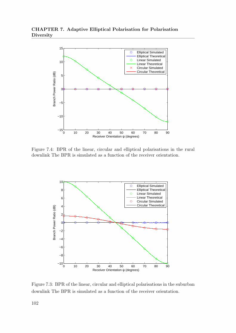
CHAPTER 7. Adaptive Elliptical Polarisation for PolarisationDiversity
0 10 20 30 40 50 60 70 80 90−15
−10
−5
0
5
10
15
Receiver Orientation ψ (degrees)
Bra
nch
Pow
er R
atio
(dB
)
Elliptical SimulatedElliptical TheoreticalLinear SimulatedLinear TheoreticalCircular SimulatedCircular Theoretical
Figure 7.4: BPR of the linear, circular and elliptical polarisations in the ruraldownlink The BPR is simulated as a function of the receiver orientation.
0 10 20 30 40 50 60 70 80 90−10
−8
−6
−4
−2
0
2
4
6
8
10
Receiver Orientation ψ (degrees)
Bra
nch
Pow
er R
atio
(dB
)
Elliptical SimulatedElliptical TheoreticalLinear SimulatedLinear TheoreticalCircular SimulatedCircular Theoretical
Figure 7.3: BPR of the linear, circular and elliptical polarisations in the suburban
downlink The BPR is simulated as a function of the receiver orientation.
102

7.1 Downlink
Simulations of the correlation coefficient as a function of the receiver orienta-
tion have also been performed for the urban, suburban and rural channel envi-
ronments. Both correlated and uncorrelated polarisation channels are examined
for each environment.
For uncorrelated polarisation channels, the simulated fading correlation co-
efficient as a function of the receiver orientation in the urban, suburban and
rural environments are presented in Fig. 7.5, Fig. 7.6 and Fig. 7.7 respectively.
Results obtained previously for linear and circular polarisation have also been
included for comparison. In can be seen across all three figures that the channel
specific elliptical polarisation is invariant to the receiver orientation and remains
uncorrelated across all orientations. The improvements gained over traditional
polarisation diversity techniques are most noticeable in the suburban and ru-
ral environments, where the correlation coefficient was reduced from 0.6694 and
0.7767 to 0.
Also of significance is that the use of circular polarisation is already optimum
the rural environment Fig. 7.7. This is an expected result since the operational
parameters for elliptical polarisation optimised to the circularly polarised signal.
0 10 20 30 40 50 60 70 80 90−0.05
0
0.05
0.1
0.15
0.2
0.25
0.3
0.35
0.4
Receiver Orientation ψ (degrees)
Cor
rela
tion
Coe
ffici
ent ρ
Simulated EllipticalTheoretical EllipticalSimulated CircularTheoretical CircularSimulated LinearTheoretical Linear
Figure 7.5: Simulation of the correlation coefficient in an uncorrelated urban
downlink. The simulation is performed as a function of the receiver orientation.
103

CHAPTER 7. Adaptive Elliptical Polarisation for PolarisationDiversity
0 10 20 30 40 50 60 70 80 90−0.1
0
0.1
0.2
0.3
0.4
0.5
0.6
0.7
Receiver Orientation ψ (degrees)
Cor
rela
tion
Coe
ffici
ent ρ
Simulated EllipticalTheoretical EllipticalSimulated CircularTheoretical CircularSimulated LinearTheoretical Linear
Figure 7.6: Simulation of the correlation coefficient in an uncorrelated suburban
downlink. The simulation is performed as a function of the receiver orientation.
0 10 20 30 40 50 60 70 80 90−0.1
0
0.1
0.2
0.3
0.4
0.5
0.6
0.7
0.8
Receiver Orientation ψ (degrees)
Cor
rela
tion
Coe
ffici
ent ρ
Simulated EllipticalTheoretical EllipticalSimulated CircularTheoretical CircularSimulated LinearTheoretical Linear
Figure 7.7: Simulation of the correlation coefficient in an uncorrelated rural down-
link. The simulation is performed as a function of the receiver orientation.
104

7.1 Downlink
0 10 20 30 40 50 60 70 80 900
0.05
0.1
0.15
0.2
0.25
0.3
0.35
0.4
0.45
Receiver Orientation ψ (degrees)
Cor
rela
tion
Coe
ffici
ent ρ
Simulated EllipticalTheoretical EllipticalSimulated CircularTheoretical CircularSimulated LinearTheoretical Linear
Figure 7.8: Simulation of the correlation coefficient in a correlated urban down-link. The simulated is performed as a function of the receiver orientation.
For correlated channels, the simulated fading correlation coefficient results are
presented in Fig. 7.8, Fig. 7.9 and Fig. 7.10 respectively. In this case, the corre-
lation coefficient is no longer receiver orientation invariant. This is an expected
outcome since the channel correlation between the cross polar links β could not
be directly controlled. Nevertheless using the channel specific elliptical polarisa-
tion maintains a power balanced XPD, which means the fading correlation now
becomes primarily a result of the channel. This implies that a fading correlation
of zero is guaranteed at the receiver orientation of ψ = 45◦, since the effect of
β is eliminated at this orientation. This feature can be observed across all three
figures. Even though the correlation coefficient could not be kept receiver orien-
tation invariant in the case of correlated channels, the results obtained are still a
significant improvement over the traditional linear polarisation based techniques.
105

CHAPTER 7. Adaptive Elliptical Polarisation for PolarisationDiversity
0 10 20 30 40 50 60 70 80 900
0.1
0.2
0.3
0.4
0.5
0.6
0.7
Receiver Orientation ψ (degrees)
Cor
rela
tion
Coe
ffici
ent ρ
Simulated EllipticalTheoretical EllipticalSimulated CircularTheoretical CircularSimulated LinearTheoretical Linear
Figure 7.9: Simulation of the correlation coefficient in a correlated suburban
downlink. The simulated is performed as a function of the receiver orientation.
0 10 20 30 40 50 60 70 80 90−0.1
0
0.1
0.2
0.3
0.4
0.5
0.6
0.7
0.8
Receiver Orientation ψ (degrees)
Cor
rela
tion
Coe
ffici
ent ρ
Simulated EllipticalTheoretical EllipticalSimulated CircularTheoretical CircularSimulated LinearTheoretical Linear
Figure 7.10: Simulation of the correlation coefficient in a correlated rural down-
link. The simulated is performed as a function of the receiver orientation.
106

7.2 Uplink
y
x
V1
V2
α
Transmitter
H11
H22
H12
H21
Hpol
Vpol
Hpol
Vpol
Channel Receiver
y
x
45◦
R1R2
Figure 7.11: Uplink polarisation diversity with elliptical polarisation.
7.2 Uplink
In the mobile uplink, the base station acts as the receiver and has a fixed orienta-
tion, while the mobile station acts as the transmitter, and has variable orientation.
The objective is therefore to derive the parameters for an elliptically polarised
signal optimised for transmitter orientation invariance.
7.2.1 System model
The mobile transmitter orientation, α is an assumed variable, and the mobile is
allowed to rotate within the xy plane. An elliptically polarised signal is transmit-
ted with antennas V1 and V2. At the base station, the orientation of the receiver
antennas are assumed to be fixed at ψ = 45◦. Fig. 7.11 illustrates this antenna
configuration.
The rationale behind using this antenna configuration was that an antenna
geometry with ψ = 45◦ guarantees power balance properties. The consequence
of an increased correlation coefficient due to a large power difference between
the vertical and horizontal polarisations or XPD need to be considered to be a
disadvantage. This is because when ψ = 45◦, the value of the fading correlation
coefficient (4.17) is primarily influenced by this power difference. Importantly,
the XPD can be controlled with an elliptically polarised signal, where as the
channel correlation parameter β is not easily controlled for ψ = 45◦.
Equation (4.17) shows that the fading correlation coefficient is optimum at 0
when the XPD to 0 dB. The primary objective therefore to derive the values of A1,
A2, and θ to achieve a power balanced XPD for any given channel. The challenge,
however, is that the XPD is transmitter orientation specific, which means there
107
CHAPTER 7. Adaptive Elliptical Polarisation for PolarisationDiversity
is no single set of operating parameters that can achieve XPD = 0 dB for all
transmitter orientations.
Nevertheless, if the condition for orientation invariance is relaxed slightly, it is
possible to achieve a 0 dB XPD that is robust to small changes in the transmitter
orientation. This is demonstrated in the following section.
7.2.2 Optimum parameters
Deriving the values of A1, A2, and θ begins with the generalised expression of the
XPD,
XPD =E[R2
y
]E [R2
x]=KdE [Γ2
21] +KsE [Γ222]
KdE [Γ211] +KsE [Γ2
12], (7.30)
where
Kd = A21 sin (α) + A2
2 cos2 (α)− 2A1A2 sin (α) cos (α) cos (θ) (7.31)
Ks = A21 cos (α) + A2
2 sin2 (α) + 2A1A2 sin (α) cos (α) cos (θ) . (7.32)
The optimisation procedure must achieve two conditions. Firstly, the value
of the XPD=0 dB at a given operating transmitter orientation α, such that,
XPD =E[R2
y
]E [R2
x]= 1 , (7.33)
and secondly, the gradient of XPD with respect to α must zero for the defined α
dXPD
dα= 0 . (7.34)
These two conditions are used to form two equations, which are used to derive a
solution for θ and the ratio between the antenna amplitudes T = A1/A2. A third
constraint is then introduced to specify the total transmitted power to finally
obtain values for A1 and A2.
The first equation is obtained through the first condition. The XPD is set to
equal 1 and the resulting expression rearranged to obtain cos (θ) as the subject.
XPD =KdE [Γ2
21] +KsE [Γ222]
KdE [Γ211] +KsE [Γ2
12]= 1 (7.35)
108

7.2 Uplink
⇒ KdE[Γ221
]+KsE
[Γ222
]= KdE
[Γ211
]+KsE
[Γ212
](7.36)
⇒E[Γ222
]− E
[Γ212
]E [Γ2
11]− E [Γ221]
=Ks
Kd=A2
1 cos (α) +A22 sin
2 (α) + 2A1A2 sin (α) cos (α) cos (θ)
A21 sin (α) +A2
2 cos2 (α)− 2A1A2 sin (α) cos (α) cos (θ)
(7.37)
Rearranging this expression for cos (θ) yields
cos (θ) =sin2 (α) (T 2 −G) + cos2 (α) (1− T 2G)
2T sin (α) cos (α) (G+ 1), (7.38)
for α = nπ2
where n is integer, and where
G =E [Γ2
22]− E [Γ212]
E [Γ211]− E [Γ2
21]. (7.39)
To obtain the second equation, the gradient of the XPD is taken with respect
to α and equated to zero. The aim is once again to obtain an equation with
cos (θ) as the subject.
dXPD
dα=E [R2
x] · ddα
{E[R2
y
]}− E
[R2
y
]· ddα
{E [R2x]}
E2 [R2x]
= 0 (7.40)
⇒E[R2
x
]· ddα
{E[R2
y
]}− E
[R2
y
]· ddα
{E[R2
x
]}= 0 (7.41)
⇒E[R2
x
]· ddα
{E[R2
y
]}= E
[R2
y
]· ddα
{E[R2
x
]}(7.42)
⇒(KdE
[Γ211
]+KsE
[Γ212
]) (K ′
dE[Γ221
]+K ′
sE[Γ222
])=(KdE
[Γ221
]+KsE
[Γ222
]) (K ′
dE[Γ211
]+K ′
sE[Γ212
])(7.43)
⇒ KdK′sE[Γ222
]E[Γ211
]+K ′
dKsE[Γ212
]E[Γ221
]= KdK
′sE[Γ212
]E[Γ221
]+K ′
dKsE[Γ222
]E[Γ211
](7.44)
109

CHAPTER 7. Adaptive Elliptical Polarisation for PolarisationDiversity
⇒K ′dKs −K ′
sKd = 0 . (7.45)
Where K ′d and K ′
s are the first derivatives of Kd and Ks with respect to α, and
are calculated as,
K ′d = 2A2
1 sin (α) cos (α)− 2A22 sin (α) cos (α)− 2A1A2 cos (θ)
(cos2 (α)− sin2 (α)
)(7.46)
K ′s = −2A2
1 sin (α) cos (α) + 2A22 sin (α) cos (α) + 2A1A2 cos (θ)
(cos2 (α)− sin2 (α)
)= −K ′
d . (7.47)
Substituting (7.47) into (7.45) and factorising, the expression simplifies to
−K ′s (Ks +Kd) = 0 , (7.48)
which means that either Ks +Kd = 0, or −K ′s = 0.
However, Ks +Kd = A21 + A2
2 = 0, which means,
K ′s = 0 (7.49)
⇒− 2A21 sin (α) cos (α) + 2A2
2 sin (α) cos (α) + 2A1A2 cos (θ)(cos2 (α)− sin2 (α)
)= 0 (7.50)
⇒T 2 sin (α) cos (α)− sin (α) cos (α)− T cos (θ) cos (2α) = 0 (7.51)
Expressing (7.51) with cos (θ) as the subject yields,
cos (θ) =sin (α) cos (α) (T 2 − 1)
T cos (2α), (7.52)
for α = π4+ 2nπ,3π
4+ 2nπ where n is integer.
Finally, the expression for T is obtained with the combination of (7.38) and
(7.52),
T =
√G sin2 (α) + cos2 (α)
sin2 (α) +G cos2 (α). (7.53)
In summary, the procedure to compute the optimal transmission parameters
is to first obtain knowledge on the transmitter orientation α and the second
order channel statistics for calculating G. The ratio of A1 to A2 is then obtained
through T in (7.53). Then, the phase offset θ is calculated from either (7.38) or
110

7.2 Uplink
(7.52), depending on the value of α. Finally, the values of A1 and A2 are obtained
after setting a constraint on the total transmit power. The parameters need to be
recalculated following changes in the channel statistics or transmitter orientation.
An example of the ideal operating parameters for mobile transmitters ori-
entated at 20◦, 40◦ and 60◦ assuming an urban environment are calculated and
summarised in Table 7.2. Diversity performance using these operating parameters
will be examined in the following results section.
α 20◦ 40◦ 60◦
T 0.7702 0.9437 1.1832
A1 0.6102 0.6863 0.7638
A2 0.7923 0.7273 0.6455
θ 1.7943 1.9059 1.8679
Table 7.2: Operating parameters for a mobile transmitter in an urban environ-
ment orientated at angles 20◦, 40◦ and 60◦.
7.2.3 Uplink results
In the mobile uplink, when the receiver orientation is set to ψ = 45◦, power
balanced is guaranteed, however the correlation coefficient becomes primarily
affected by the XPD. The objective in the uplink was to optimise the transmission
parameters to achieve an orientation invariant XPD equal to 0 dB at a given
transmitter orientation and a given set of channel statistics.
For an urban environment with the transmitter orientations at 20◦, 40◦ and
60◦, the operation parameters A1, A2 and θ have been calculated and summarised
in Table 7.2. Simulation results of the XPD for each of these three systems as a
function of the transmitter orientation in the urban environment are illustrated
in Fig. 7.12. At the respective transmitter orientations, the XPD is optimally
power balanced and also resides at a local minimum. This means that changes in
the transmitter orientation will not induce large changes in the XPD. For example
the XPD does not increase by more than 0.12 dB following a ±10◦ deviation from
the operating orientation.
Simulations for the fading correlation coefficient as a function of the transmit-
ter orientation in uncorrelated and correlated channels are presented in Fig. 7.13
and Fig. 7.14 respectively. Once again, the operating parameters, optimised for
111

CHAPTER 7. Adaptive Elliptical Polarisation for PolarisationDiversity
0 10 20 30 40 50 60 70 80 90−0.5
0
0.5
1
1.5
2
2.5
3
Transmitter Orientation α (degrees)
XP
D (
dB)
A1=0.6863, A
2=0.7273, θ=1.9059
A1= 0.7638, A
2=0.6455, θ=1.8679
A1=0.6102, A
2=0.7923, θ=1.7943
Figure 7.12: Uplink simulation of the XPD as a function of the transmitter orien-tation in an urban environment. The three systems plotted have their parametersoptimised at transmitter orientations of 20◦, 40◦ and 60◦.
transmitter orientations 20◦, 40◦ and 60◦ as summarised in Table 7.2 were used
for the simulation. With the fading correlation coefficient being chiefly affected
by the XPD when the receiver orientation is fixed to ψ = 45◦, and coupled with
the demonstration in Fig. 7.12 that the XPD was power balanced and robust
to changes in the transmitter orientation means the fading correlation coefficient
should also be optimum and robust to orientation. This reasoning is substanti-
ated by the simulations for both types of channels, demonstrating the ideal and
robust nature of the fading correlation coefficient when channel specific elliptically
polarised signals optimised for diversity are used.
There appears to be little difference between the simulated results of the
correlated and uncorrelated channels, with correlated channels yielding a slightly
lower result. This is to be expected since the channel correlation parameter β
has little influence over the correlation coefficient at ψ = 45◦. The reason for this
is that β resides in the denominator of (7.2), and therefore slightly reduces the
fading correlation coefficient in correlated channels, where β = 0.
112
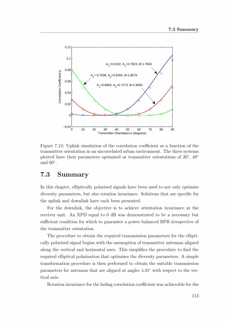
7.3 Summary
0 10 20 30 40 50 60 70 80 90−0.02
0
0.02
0.04
0.06
0.08
0.1
0.12
Transmitter Orientation α (degrees)
Cor
rela
tion
Coe
ffici
ent ρ
A1= 0.7638, A
2=0.6455, θ=1.8679
A1=0.6102, A
2=0.7923, θ=1.7943
A1=0.6863, A
2=0.7273, θ=1.9059
Figure 7.13: Uplink simulation of the correlation coefficient as a function of thetransmitter orientation in an uncorrelated urban environment. The three systemsplotted have their parameters optimised at transmitter orientations of 20◦, 40◦
and 60◦.
7.3 Summary
In this chapter, elliptically polarised signals have been used to not only optimise
diversity parameters, but also rotation invariance. Solutions that are specific for
the uplink and downlink have each been presented.
For the downlink, the objective is to achieve orientation invariance at the
receiver unit. An XPD equal to 0 dB was demonstrated to be a necessary but
sufficient condition for which to guarantee a power balanced BPR irrespective of
the transmitter orientation.
The procedure to obtain the required transmission parameters for the ellipti-
cally polarised signal begins with the assumption of transmitter antennas aligned
along the vertical and horizontal axes. This simplifies the procedure to find the
required elliptical polarisation that optimises the diversity parameters. A simple
transformation procedure is then performed to obtain the suitable transmission
parameters for antennas that are aligned at angles ±45◦ with respect to the ver-
tical axis.
Rotation invariance for the fading correlation coefficient was achievable for the
113

CHAPTER 7. Adaptive Elliptical Polarisation for PolarisationDiversity
0 10 20 30 40 50 60 70 80 90−0.02
0
0.02
0.04
0.06
0.08
0.1
0.12
Transmitter Orientation α (degrees)
Cor
rela
tion
Coe
ffici
ent ρ
A1= 0.7638, A
2=0.6455, θ=1.8679
A1=0.6863, A
2=0.7273, θ=1.9059
A1=0.6102, A
2=0.7923, θ=1.7943
Figure 7.14: Uplink simulation of the correlation coefficient as a function of thetransmitter orientation in a correlated urban environment. The three systemsplotted have their parameters optimised at transmitter orientations of 20◦, 40◦
and 60◦.
uncorrelated channel, but not the correlated channel. This was due to the fact
that the channel correlation coefficient β could not be easily controlled. Despite
this, values of the fading correlation coefficient were shown to be very low, and
outperforms polarisation diversity systems that transmit circularly and linearly
polarised signals.
For the mobile uplink, the objective is to achieve orientation invariance at the
transmitter unit. The base station receiver orientation is set to ψ = 45◦, so that
a power balanced BPR can be guaranteed. A second but more significant reason
for such assignment is that the fading correlation coefficient becomes primarily
influenced by the XPD, which can be easily controlled. This therefore allows the
fading correlation coefficient to be controlled and optimised.
The transmitter parameters to generate the required elliptically polarised sig-
nal are calculated using second order statistics of the polarisation channel and
the current transmitter antenna orientation. The resulting fading correlation co-
efficient is not strictly orientation invariant, but has been designed to be robust
to moderate changes in the transmitter orientation.
114

7.3 Summary
The most significant disadvantage of using elliptical polarisation for diversity
is that it requires the estimation of the second order channel statistics. Param-
eters need to be updated periodically to account for changes in the channel.
Specific to the uplink, an estimation for the transmitter orientation is also re-
quired.
115


Chapter 8
Conclusion and future research
Multipath fading adversely effects mobile communication because erratic vari-
ations in signal intensity across short distances degrades communication qual-
ity and interferes with signal detection. Diversity techniques counteract fad-
ing by combining multiple signals affected by independent channel conditions to
minimise the occurrence and duration of signal nulls. A reduction in fading is
achieved because the probability of a deep fade occurring simultaneously across
all branches is significantly less than a fade experienced by any individual branch.
Signal diversity can be achieved in the time, frequency and spatial domains.
Spatial domain techniques uses multiple independent antenna elements to cap-
ture diversity signals, and are popular because diversity signals can be captured
without the need for additional allocations of spectra. However, the physical di-
mensions required by some types of space diversity are infeasible for terrestrial
mobile communications.
Polarisation diversity is a subset of spatial diversity which allows for very
compact antenna profiles. This kind of diversity exploits signals residing across
orthogonal polarisations for diversity purposes which means antenna elements
can be mounted in close proximity.
Ideally, diversity requires that two or more independently captured signals
have low fading correlation and equal average branch powers. Diversity perfor-
mance becomes severely limited when the fading correlation coefficient exceeds
0.7 or exhibits an average branch power imbalance in excess of 6 dB. Traditional
implementations of polarisation diversity can capture diversity signals with very
low fading correlation, but generally exhibit significant levels of average power
imbalance. The level of imbalance often exceeds this threshold, especially in the
CHAPTER 8. Conclusion and future research
suburban and rural environments. Because of this, polarisation diversity is gen-
erally avoided in favour of spatial diversity, and only used if absolutely necessary.
The function of polarisation diversity was also found to be sensitive to an-
tenna orientation both at the transmitter and receiver side. Acceptable diversity
parameters achieved for a particular antenna geometry does not automatically
imply that they will remain this way for another orientation. This introduces a
further challenge for terrestrial mobile communications since cellular phones are
hand held devices and can assume arbitrary and variable orientations.
The implications of the power imbalance problem was explored in Chapter
3, where polarisation diversity was combined with the MC-CDMA scheme. The
findings of this research challenged the acceptable bounds for diversity parame-
ters and demonstrated that performance improvements were only possible if the
average power imbalance was less than 3 dB. The presence of diversity with higher
levels of power imbalance was observed to have an adverse effect on system per-
formance. Results demonstrate that it is better to have no diversity, rather than
one that performs poorly. This highlights the importance for the proper deploy-
ment of diversity systems to capture signals that have low fading correlation and
equal average branch powers.
In making polarisation diversity a more successful antenna diversity tech-
nique, this research developed a generalised polarisation model that accounts for
the transmitter orientation, the receiver orientation, and also the possibility of
correlated polarisation channels. This is presented in Chapter 4, and also derives
the generalised expressions for the branch power ratio and the fading correlation
coefficient. This development allowed a more detailed insight into the factors
contributing to the large power imbalance and its interactions with the fading
correlation coefficient.
The traditional implementation of polarisation diversity with diversity anten-
nas at the receiver aligned along the vertical and horizontal axes was revisited in
Chapter 5 to complete a thorough treatment on the effects of antenna orientations.
Both the uplink and downlink scenarios were examined using the mathematical
model developed in Chapter 4. The variation of the diversity parameters as a
function of both the transmitter and receiver orientations were simulated. The
variation of the BPR was observed to be particularly severe in the suburban and
rural environments.
For the mobile uplink, average branch power balance could be achieved by
118

8 Conclusion and future research
aligning the transmitter antenna to a calculated optimum orientation. However,
the power balance is easily disturbed following small changes in the transmitter
orientation. Since it is unrealistic to expect a mobile transmitter to remain in a
fixed orientation, this mode of polarisation diversity is not suitable for the uplink.
Addressing the large power imbalance from the receiver end of the mobile
downlink can be achieved with the use of an antenna geometry that is symmetric
at ±45◦ relative to the vertical axis. However, the balanced average branch power
is achieved at the expense of an increased correlation coefficient. A large power
imbalance between the vertical and horizontal polarisations converts to a high
fading correlation coefficient that often exceeds the 0.7 threshold required for
effective diversity.
Excessive increases in the fading correlation were identified to be caused by a
large XPD. Chapter 6 explores the use of circularly polarised signals to reduce the
XPD. The rationale behind using circular polarisation is that there is component
of the electric field in every direction in the plane orthogonal to the direction of
propagation. This encourages power coupling between the vertical and horizon-
tal polarisations and therefore promotes the conditions for a lower XPD. Using
circular polarisation for polarisation diversity is a significant improvement over
traditional linear polarisation based diversity techniques. Nevertheless, the re-
sults obtained for the branch power ratio and the correlation coefficient indicate
that performance is dictated by the channel, and therefore generally suboptimal.
Optimising polarisation diversity to achieve diversity branches that exhibit
power balance, zero fading correlation and simultaneously negates the effects of
antenna rotation is presented in Chapter 7. The solution is to use a combination of
specialised antenna geometries and channel specific elliptically polarised signals.
Since the requirements for rotation invariance in the uplink and downlink are
different, independent solutions have been presented.
In the mobile downlink, orientation invariance is required at the mobile re-
ceiver. A necessary but sufficient condition to guarantee a power balanced BPR
irrespective of the receiver orientation was to achieve and maintain XPD = 0 dB.
The procedure to calculate the required operating parameters for the elliptical
polarisation begins with the derivation of the required elliptically polarised signal
that achieves a 0 dB XPD with transmitter antennas aligned along the vertical
and horizontal axes. A simple transformation is then applied to obtain the op-
erating parameters for transmitter antennas aligned at angles ±45◦ with respect
119

CHAPTER 8. Conclusion and future research
to the vertical axis.
For the mobile uplink, rotation invariance is required at the mobile trans-
mitter. In this scenario, the base station receiver must assume an orientation
of ψ = 45◦. This not only guarantees a power balanced BPR, but more im-
portantly, allows the fading correlation coefficient to be controlled via the XPD.
The transmission parameters for the elliptically polarised signal are calculated
using the second order polarisation channel statistics and the current transmitter
orientation to satisfy an XPD of 0 dB and a stationary gradient with respect to
the transmitter orientation. This scheme, though optimum, is not strictly rota-
tion invariant. Diversity parameters, however, are robust to moderate changes in
transmitter orientation.
Using the channel specific elliptically polarised signals provides the optimum
conditions for polarisation diversity to counteract fading, and are significant im-
provements over traditional polarisation diversity techniques using linearly and
circularly polarised signals. The outcomes of this research enhances the perfor-
mance of polarisation diversity and promotes greater reliability in mobile com-
munications.
8.0.1 Future research
Calculating the suitable transmission parameters for the channel specific ellipti-
cally polarised signals requires the knowledge of the second order statistics of the
polarisation channel. The fact that this knowledge is required at the transmitter
side introduces further challenges. While the availability of the channel statistics
is not as time critical as the instantaneous channel state information, accurate
knowledge is still required to ensure optimum diversity performance.
While the research conducted by this thesis have demonstrated an optimised
performance when perfect knowledge of the polarisation channel statistics are
available, effects of incorrect channel estimations have not been investigated.
Analysing how the diversity parameters will behave in the presence of noisy chan-
nel statistics therefore constitutes the next logical step for future research.
Also of particular interest is to determine exactly how often the operating
parameters of the ellipse need to be recalculated. Since it is the second order
channel statistics that are required, and not the instantaneous channel state in-
formation, the update frequency need not occur as frequently as the coherence
time. Perhaps a more suitable time frame would be in the order of 30 to 120
120

8 Conclusion and future research
wavelengths to allow the second order statistics to be properly observed. For a
mobile station operating at 1.2GHz travelling at 60km/hr, this translates into a
time frame of 450ms to 1.8s respectively.
A recalculation of the ellipse parameters, however, should definitely occur if
the mobile unit detects a significant antenna rotation.
121


Appendix A
Power Correlation Coefficient for
the Generalised Polarisation
Diversity Model
This appendix presents the derivation of the correlation coefficient for the gener-
alised polarisation diversity system described in Chapter 4.
The expression for the power correlation coefficient between antenna branches
R1 and R2 is defined as the covariance of R21 and R2
2, normalised by the product
of their respective standard deviations,
ρp =E [R2
1R22]− E [R2
1]E [R22]√
(E [R41]− E2 [R2
1]) (E [R42]− E2 [R2
2]). (A.1)
The objective is to calculate the required moments and joint moments of R1 and
R2, and then substitute them back into (A.1).
First the expressions for R1 and R2 must be obtained. Mathematically, they
are evaluated through the multiplication of the receiver rotation matrix, the chan-
nel matrix, the transmitter rotation matrix and the transmit signal vector. This
model has been presented in Chapter 4.
R1
R2
=
sin (ψ) cos (ψ)
− cos (ψ) sin (ψ)
Γ11ejϕ11 Γ12e
jϕ12
Γ21ejϕ21 Γ22e
jϕ22
sin (α) − cos (α)
cos (α) sin (α)
A1ejωt
A2ej(ωt−θ)
.(A.2)
The received signal vector [R1R2]T can alternatively be expressed in terms of the

APPENDIX A. Power Correlation Coefficient for the GeneralisedPolarisation Diversity Model
Rx and Ry which are the signals residing in the vertical and horizontal polarisa-
tions, respectively, after the channel,[R1
R2
]=
[sin (ψ) cos (ψ)
− cos (ψ) sin (ψ)
][Rx
Ry
](A.3)
where[Rx
Ry
]=
[Γ11e
jϕ11 Γ12ejϕ12
Γ21ejϕ21 Γ22e
jϕ22
][sin (α) − cos (α)
cos (α) sin (α)
][A1e
jωt
A2ej(ωt−θ)
]. (A.4)
A.1 Moments E[R2
1
]and E
[R2
2
][R1
R2
]=
[Rx sin (ψ) +Ry cos (ψ)
−Rx cos (ψ) +Ry sin (ψ)
](A.5)
R21 = R1 ×R∗
1
= [Rx sin (ψ) +Ry cos (ψ)][R∗
x sin (ψ) +R∗y cos (ψ)
]= R2
x sin2 (ψ) +R2
y cos2 (ψ) + sin (ψ) cos (ψ)
(RxR
∗y +R∗
xRy
)(A.6)
R22 = R2 ×R∗
2
= [−Rx cos (ψ) +Ry sin (ψ)][−R∗
x cos (ψ) +R∗y sin (ψ)
]= R2
x cos2 (ψ) +R2
y sin2 (ψ)− sin (ψ) cos (ψ)
(RxR
∗y +R∗
xRy
)(A.7)
E[R2
1
]= E
[R2
x
]sin2 (ψ) + E
[R2
y
]cos2 (ψ) + sin (ψ) cos (ψ)E
[RxR
∗y +R∗
xRy
](A.8)
E[R2
2
]= E
[R2
x
]cos2 (ψ) + E
[R2
y
]sin2 (ψ)− sin (ψ) cos (ψ)E
[RxR
∗y +R∗
xRy
](A.9)
The moments E [R2x], E [Ry] and E
[RxR
∗y +R∗
xRy
]are required.
124

A.1 Moments E [R21] and E [R2
2]
A.1.1 Moments E[R2x
]and E
[R2y
]Rx =A1Γ11 sin (α) e
j(ωt+ϕ11) − A2Γ11 cos (α) ej(ωt−θ+ϕ11)
+ A1Γ12 cos (α) ej(ωt+ϕ12) + A2Γ12 sin (α) e
j(ωt−θ+ϕ12) (A.10)
Ry =A1Γ21 sin (α) ej(ωt+ϕ21) − A2Γ21 cos (α) e
j(ωt−θ+ϕ21)
+ A1Γ22 cos (α) ej(ωt+ϕ22) + A2Γ22 sin (α) e
j(ωt−θ+ϕ22) (A.11)
R2x = A2
1Γ211 sin
2 (α) + A22Γ
211 cos
2 (α) + A21Γ
212 cos
2 (α) + A21Γ
212 sin
2 (α)
− 2A1A2Γ211 sin (α) cos (α) cos (θ) + 2A2
1Γ11Γ12 sin (α) cos (α) cos (ϕ11 − ϕ12)
+ 2A1A2Γ212 sin (α) cos (α) cos (θ)− 2A2
2Γ11Γ12 sin (α) cos (α) cos (ϕ11 − ϕ12)
+ 2A1A2Γ11Γ12 sin2 (α) cos (ϕ11 − ϕ12 + θ)
− 2A1A2Γ11Γ12 cos2 (α) cos (ϕ11 − ϕ12 − θ) (A.12)
= Γ211
(A2
1 sin2 (α) + A2
2 cos2 (α)− 2A1A2 sin (α) cos (α) cos (θ)
)+ Γ2
12
(A2
1 cos2 (α) + A2
2 sin2 (α) + 2A1A2 sin (α) cos (α) cos (θ)
)+ 2A2
1Γ11Γ12 sin (α) cos (α) cos (ϕ11 − ϕ12)
− 2A22Γ11Γ12 sin (α) cos (α) cos (ϕ11 − ϕ12)
+ 2A1A2Γ11Γ12 sin2 (α) cos (ϕ11 − ϕ12) cos (θ)
− 2A1A2Γ11Γ12 sin2 (α) sin (ϕ11 − ϕ12) sin (θ)
− 2A1A2Γ11Γ12 cos2 (α) cos (ϕ11 − ϕ12) cos (θ)
− 2A1A2Γ11Γ12 cos2 (α) sin (ϕ11 − ϕ12) sin (θ) (A.13)
= Γ211Kd + Γ2
12Ks + 2Γ11Γ12 cos (ϕ11 − ϕ12)KA − 2Γ11Γ12 sin (ϕ11 − ϕ12)KB
(A.14)
where
Kd = A21 sin
2 (α) + A22 cos
2 (α)− 2A1A2 sin (α) cos (α) cos (θ) (A.15)
Ks = A21 cos
2 (α) + A22 sin
2 (α) + 2A1A2 sin (α) cos (α) cos (θ) (A.16)
KA = A21 sin (α) cos (α)− A2
2 sin (α) cos (α)
+ A1A2 sin2 (α) cos (θ)− A1A2 cos
2 (α) cos (θ) (A.17)
125

APPENDIX A. Power Correlation Coefficient for the GeneralisedPolarisation Diversity Model
KB = A1A2 sin (θ) (A.18)
R2y = A2
1Γ221 sin
2 (α) + A22Γ
221 cos
2 (α) + A21Γ
222 cos
2 (α) + A22Γ
222 sin
2 (α)
− 2A1A2Γ221 sin (α) cos (α) cos (θ) + 2A2
1Γ21Γ22 sin (α) cos (α) cos (ϕ21 − ϕ22)
+ 2A1A2Γ222 sin (α) cos (α) cos (θ)− 2A2
2Γ21Γ22 sin (α) cos (α) cos (ϕ21 − ϕ22)
+ 2A1A2Γ21Γ22 sin2 (α) cos (ϕ21 − ϕ22 + θ)
− 2A1A2Γ21Γ22 cos2 (α) cos (ϕ21 − ϕ22 − θ) (A.19)
= Γ221
(A2
1 sin2 (α) + A2
2 cos2 (α)− 2A1A2 sin (α) cos (α) cos (θ)
)+ Γ2
22
(A2
1 cos2 (α) + A2
2 sin2 (α) + 2A1A2 sin (α) cos (α) cos (θ)
)+ 2A2
1Γ21Γ22 sin (α) cos (α) cos (ϕ21 − ϕ22)
− 2A22Γ21Γ22 sin (α) cos (α) cos (ϕ21 − ϕ22)
+ 2A1A2Γ21Γ22 sin2 (α) cos (ϕ21 − ϕ22) cos (θ)
− 2A1A2Γ21Γ22 sin2 (α) sin (ϕ21 − ϕ22) sin (θ)
− 2A1A2Γ21Γ22 cos2 (α) cos (ϕ21 − ϕ22) cos (θ)
− 2A1A2Γ21Γ22 cos2 (α) sin (ϕ21 − ϕ22) sin (θ) (A.20)
= Γ221Kd + Γ2
22Ks + 2Γ21Γ22 cos (ϕ21 − ϕ22)KA − 2Γ21Γ22 sin (ϕ21 − ϕ22)KB
(A.21)
E[R2
x
]=KdE
[Γ211
]+KsE
[Γ212
](A.22)
E[R2
y
]=KdE
[Γ221
]+KsE
[Γ222
](A.23)
A.1.2 Moment E[RxR
∗y +R∗
xRy
]RxR
∗y +R∗
xRy = 2R{RxR
∗y
}= 2R
{(A1Γ11 sin (α) e
j(ωt+ϕ11) − A2Γ11 cos (α) ej(ωt−θ+ϕ11)
+A1Γ12 cos (α) ej(ωt+ϕ12) + A2Γ12 sin (α) e
j(ωt−θ+ϕ12))
×(A1Γ21 sin (α) e
−j(ωt+ϕ21) − A2Γ21 cos (α) e−j(ωt−θ+ϕ21)
+A1Γ22 cos (α) e−j(ωt+ϕ22) + A2Γ22 sin (α) e
−j(ωt−θ+ϕ22))}
(A.24)
126

A.2 Joint Moment E [R21R
22]
R{RxR
∗y
}= A2
1Γ11Γ21 sin2 (α) cos (ϕ11 − ϕ21)
− A1A2Γ11Γ21 sin (α) cos (α) cos (ϕ11 − ϕ21 + θ)
+ A21Γ11Γ22 sin (α) cos (α) cos (ϕ11 − ϕ22)
+ A1A2Γ11Γ22 sin2 (α) cos (ϕ11 − ϕ22 + θ)
− A1A2Γ11Γ21 sin (α) cos (α) cos (ϕ11 − ϕ21 − θ)
+ A22Γ11Γ21 cos
2 (α) cos (ϕ11 − ϕ21)
− A1A2Γ11Γ22 cos2 (α) cos (ϕ11 − ϕ22 − θ)
− A22Γ11Γ22 sin (α) cos (α) cos (ϕ11 − ϕ22)
+ A21Γ12Γ21 sin (α) cos (α) cos (ϕ12 − ϕ21)
− A1A2Γ12Γ21 cos2 (α) cos (ϕ12 − ϕ21 + θ)
+ A21Γ12Γ22 cos
2 (α) cos (ϕ12 − ϕ22)
+ A1A2Γ12Γ22 sin (α) cos (α) cos (ϕ12 − ϕ22 + θ)
+ A1A2Γ12Γ21 sin2 (α) cos (ϕ12 − ϕ21 − θ)
− A22Γ12Γ21 sin (α) cos (α) cos (ϕ12 − ϕ21)
+ A1A2Γ12Γ22 sin (α) cos (α) cos (ϕ12 − ϕ22 + θ)
+ A22Γ12Γ22 sin
2 (α) cos (ϕ12 − ϕ22) (A.25)
= Γ11Γ21 cos (ϕ11 − ϕ21)Kd + Γ12Γ22 cos (ϕ12 − ϕ22)Ks
+ Γ11Γ22 cos (ϕ11 − ϕ22)KA + Γ12Γ21 cos (ϕ12 − ϕ21)KA
− Γ11Γ22 sin (ϕ11 − ϕ22)KB + Γ12Γ21 sin (ϕ12 − ϕ21)KB (A.26)
E[RxR
∗y +R∗
xRy
]= 2E
[R{RxR
∗y
}]= 0 (A.27)
A.2 Joint Moment E[R2
1R22
]R2
1R22 =
(R2
x sin2 (ψ) +R2
y cos2 (ψ) + sin (ψ) cos (ψ)
(RxR
∗y +R∗
xRy
))×(R2
x cos2 (ψ) +R2
y sin2 (ψ)− sin (ψ) cos (ψ)
(RxR
∗y +R∗
xRy
))(A.28)
127

APPENDIX A. Power Correlation Coefficient for the GeneralisedPolarisation Diversity Model
R21R
22 = R4
x sin2 (ψ) cos2 (ψ) +R2
xR2y sin
4 (ψ)− sin3 (ψ) cos (ψ)R2x
(RxR
∗y +R∗
xRy
)+R2
xR2y cos
4 (ψ) +R4y sin
2 (ψ) cos2 (ψ)
− sin (ψ) cos3 (ψ)R2y
(RxR
∗y +R∗
xRy
)+ sin (ψ) cos3 (ψ)R2
x
(RxR
∗y +R∗
xRy
)+ sin3 (ψ) cos (ψ)R2
y
(RxR
∗y +R∗
xRy
)− sin2 (ψ) cos2 (ψ)
(RxR
∗y +R∗
xRy
)2(A.29)
E[R2
1R22
]= sin2 (ψ) cos2 (ψ)E
[R4
x
]+ sin4 (ψ)E
[R2
xR2y
]+ cos4 (ψ)E
[R2
xR2y
]+ sin2 (ψ) cos2 (ψ)E
[R4
y
]− sin2 (ψ) cos2 (ψ)E
[(RxR
∗y +R∗
xRy
)2]− sin3 (ψ) cos (ψ)E
[R2
x
(RxR
∗y +R∗
xRy
)]− sin (ψ) cos3 (ψ)E
[R2
y
(RxR
∗y +R∗
xRy
)]+ sin (ψ) cos3 (ψ)E
[R2
x
(RxR
∗y +R∗
xRy
)]+ sin3 (ψ) cos (ψ)E
[R2
y
(RxR
∗y +R∗
xRy
)](A.30)
The following moments are required:
• E [R4x]
• E[R4
y
]• E
[R2
xR2y
]• E
[R2
x
(RxR
∗y +R∗
xRy
)]• E
[R2
y
(RxR
∗y +R∗
xRy
)]• E
[(RxR
∗y +R∗
xRy
)2]A.2.1 Moment E
[R4x
]R4
x =(R2
x
)2(A.31)
128

A.2 Joint Moment E [R21R
22]
R2x = Γ2
11Kd + Γ212Ks + 2Γ11Γ12 cos (ϕ11 − ϕ12)KA − 2Γ11Γ12 sin (ϕ11 − ϕ12)KB
(A.32)
R4x = Γ4
11K2d + 2Γ2
11Γ212KdKs + 4Γ3
11Γ12 cos (ϕ11 − ϕ12)KAKd + Γ412K
2s
− 4Γ311Γ12 sin (ϕ11 − ϕ12)KBKd + 4Γ11Γ
312 cos (ϕ11 − ϕ12)KAKs
− 4Γ11Γ312 sin (ϕ11 − ϕ12)KBKs + 4Γ2
11Γ212 cos
2 (ϕ11 − ϕ12)K2A
− 8Γ211Γ
212 sin (ϕ11 − ϕ12) cos (ϕ11 − ϕ12)KAKB
+ 4Γ211Γ
212 sin
2 (ϕ11 − ϕ12)K2B (A.33)
E[R4
x
]= E
[Γ411
]K2
d + E[Γ412
]K2
s + 2E[Γ211
]E[Γ212
]KdKs
+ 2E[Γ211
]E[Γ212
]K2
A + 2E[Γ211
]E[Γ212
]K2
B (A.34)
= 2E2[Γ211
]K2
d + 2E2[Γ212
]K2
s + 4E[Γ211
]E[Γ212
]KdKs
− 2E[Γ211
]E[Γ212
]KdKs + 2E
[Γ211
]E[Γ212
]K2
A + 2E[Γ211
]E[Γ212
]K2
B
(A.35)
E[R4
x
]= 2E2
[R2
x
]+ 2E
[Γ211
]E[Γ212
] (K2
A +K2B −KdKs
)(A.36)
A.2.2 Moment E[R4y
]
R4y =
(R2
y
)2(A.37)
R2y = Γ2
21Kd + Γ222Ks + 2Γ21Γ22 cos (ϕ21 − ϕ22)KA − 2Γ21Γ22 sin (ϕ21 − ϕ22)KB
(A.38)
129

APPENDIX A. Power Correlation Coefficient for the GeneralisedPolarisation Diversity Model
R4y = Γ4
21K2d + 2Γ2
21Γ222KdKs + 4Γ3
21Γ22 cos (ϕ21 − ϕ22)KAKd + Γ422K
2s
− 4Γ321Γ22 sin (ϕ21 − ϕ22)KBKd + 4Γ21Γ
322 cos (ϕ21 − ϕ22)KAKs
− 4Γ21Γ322 sin (ϕ21 − ϕ22)KBKs + 4Γ2
21Γ222 cos
2 (ϕ21 − ϕ22)K2A
− 8Γ221Γ
222 sin (ϕ21 − ϕ22) cos (ϕ21 − ϕ22)KAKB
+ 4Γ221Γ
222 sin
2 (ϕ21 − ϕ22)K2B (A.39)
E[R4
y
]= E
[Γ421
]K2
d + E[Γ422
]K2
s + 2E[Γ221
]E[Γ222
]KdKs
+ 2E[Γ221
]E[Γ222
]K2
A + 2E[Γ221
]E[Γ222
]K2
B (A.40)
= 2E2[Γ221
]K2
d + 2E2[Γ222
]K2
s + 4E[Γ221
]E[Γ222
]KdKs
− 2E[Γ221
]E[Γ222
]KdKs + 2E
[Γ221
]E[Γ222
]K2
A + 2E[Γ221
]E[Γ222
]K2
B
(A.41)
E[R4
y
]= 2E2
[R2
y
]+ 2E
[Γ221
]E[Γ222
] (K2
A +K2B −KdKs
)(A.42)
Simplification of K2A +K2
B −KdKs
K2A =
(A2
1 sin (α) cos (α)− A22 sin (α) cos (α)
+A1A2 sin2 (α) cos (θ)− A1A2 cos
2 (α) cos (θ)
)2
(A.43)
K2A = A4
1 sin2 (α) cos2 (α) + A4
2 sin2 (α) cos2 (α)
+ A21A
22 sin
4 (α) cos2 (α) + A21A
22 cos
4 (α) cos2 (α)
− 2A21A
22 sin
2 (α) cos2 (α)
+ 2A31A2 sin
3 (α) cos (α) cos (θ)− 2A31A2 sin (α) cos
3 (α) cos (θ)
− 2A1A32 sin
3 (α) cos (α) cos (θ) + 2A1A32 sin (α) cos
3 (α) cos (θ)
− 2A21A
22 sin
2 (α) cos2 (α) cos2 (θ) (A.44)
K2B = A2
1A22 sin
2 (θ) (A.45)
130

A.2 Joint Moment E [R21R
22]
KdKs =(A2
1 sin2 (α) + A2
2 cos2 (α)− 2A1A2 sin (α) cos (α) cos (θ)
)×(A2
1 cos2 (α) + A2
2 sin2 (α) + 2A1A2 sin (α) cos (α) cos (θ)
)(A.46)
= A41 sin
2 (α) cos2 (α) + A21A
22 sin
4 (α) + 2A31A2 sin
3 (α) cos (α) cos (θ)
+ A21A
22 cos
4 (α) + A42 sin
2 (α) cos2 (α) + 2A1A32 sin (α) cos
3 (α) cos (θ)
− 2A31A2 sin (α) cos
3 (α) cos (θ)− 2A1A32 sin
3 (α) cos (α) cos (θ)
− 4A21A
22 sin
2 (α) cos2 (α) cos2 (θ) (A.47)
K2A +K2
B −KdKs
= A21A
22 sin
4 (α) cos2 (θ) + A21A
22 cos
4 (α) cos2 (θ)
+ 2A21A
22 sin
2 (α) cos2 (α) cos2 (θ)
− A21A
22 sin
4 (α)− A21A
22 cos
4 (α)− 2A21A
22 sin
2 (α) cos2 (α)
+ A21A
22 sin
2 (θ) (A.48)
= A21A
22 cos
2 (θ)(sin2 (α) + cos2 (α)
)2+ A2
1A22 sin
2 (θ)
− A21A
22
(sin2 (α) + cos2 (α)
)2(A.49)
= A21A
22 − A2
1A22 (A.50)
K2A +K2
B −KdKs = 0 (A.51)
conversely,
K2A +K2
B = KdKs (A.52)
131

APPENDIX A. Power Correlation Coefficient for the GeneralisedPolarisation Diversity Model
A.2.3 Moment E[R2xR
2y
]
R2xR
2y =
(Γ211Kd + Γ2
12Ks + 2Γ11Γ12 cos (ϕ11 − ϕ12)KA
−2Γ11Γ12 sin (ϕ11 − ϕ12)KB
)
×
(Γ221Kd + Γ2
22Ks + 2Γ21Γ22 cos (ϕ21 − ϕ22)KA
−2Γ21Γ22 sin (ϕ21 − ϕ22)KB
)(A.53)
R2xR
2y = Γ2
11Γ221K
2d + Γ2
11Γ222KdKs + Γ2
12Γ221KdKs + Γ2
12Γ222K
2s
+ 2Γ211Γ21Γ22 cos (ϕ21 − ϕ22)KAKd − 2Γ2
11Γ21Γ22 sin (ϕ21 − ϕ22)KBKd
+ 2Γ212Γ21Γ22 cos (ϕ21 − ϕ22)KAKs − 2Γ2
12Γ21Γ22 sin (ϕ21 − ϕ22)KBKs
+ 2Γ221Γ11Γ12 cos (ϕ11 − ϕ12)KAKd + 2Γ2
22Γ11Γ12 cos (ϕ11 − ϕ12)KAKs
+ 4Γ11Γ12Γ21Γ22 cos (ϕ11 − ϕ12) cos (ϕ21 − ϕ22)K2A
− 4Γ11Γ12Γ21Γ22 cos (ϕ11 − ϕ12) sin (ϕ21 − ϕ22)KAKB
− 2Γ221Γ11Γ12 sin (ϕ11 − ϕ12)KBKd − 2Γ2
22Γ11Γ12 sin (ϕ11 − ϕ12)KBKs
− 4Γ11Γ12Γ21Γ22 sin (ϕ11 − ϕ12) cos (ϕ21 − ϕ22)KAKB
+ 4Γ11Γ12Γ21Γ22 sin (ϕ11 − ϕ12) sin (ϕ21 − ϕ22)K2B (A.54)
E[R2
xR2y
]= K2
dE[Γ211Γ
221
]+KdKsE
[Γ211
]E[Γ222
]+KdKsE
[Γ212
]E[Γ221
]+K2
sE[Γ212Γ
222
](A.55)
A.2.4 Moment E[R2x
(RxR
∗y +R∗
xRy
)]R2
x
(RxR
∗y +R∗
xRy
)=(
Γ211Kd + Γ2
12Ks + 2Γ11Γ12 cos (ϕ11 − ϕ12)KA − 2Γ11Γ12 sin (ϕ11 − ϕ12)KB
)× (Γ11Γ21 cos (ϕ11 − ϕ21)Kd + Γ12Γ22 cos (ϕ12 − ϕ22)Ks
+ Γ11Γ22 cos (ϕ11 − ϕ22)KA + Γ12Γ21 cos (ϕ12 − ϕ21)KA
−Γ11Γ22 sin (ϕ11 − ϕ22)KB + Γ12Γ21 sin (ϕ12 − ϕ21)KB) (A.56)
132
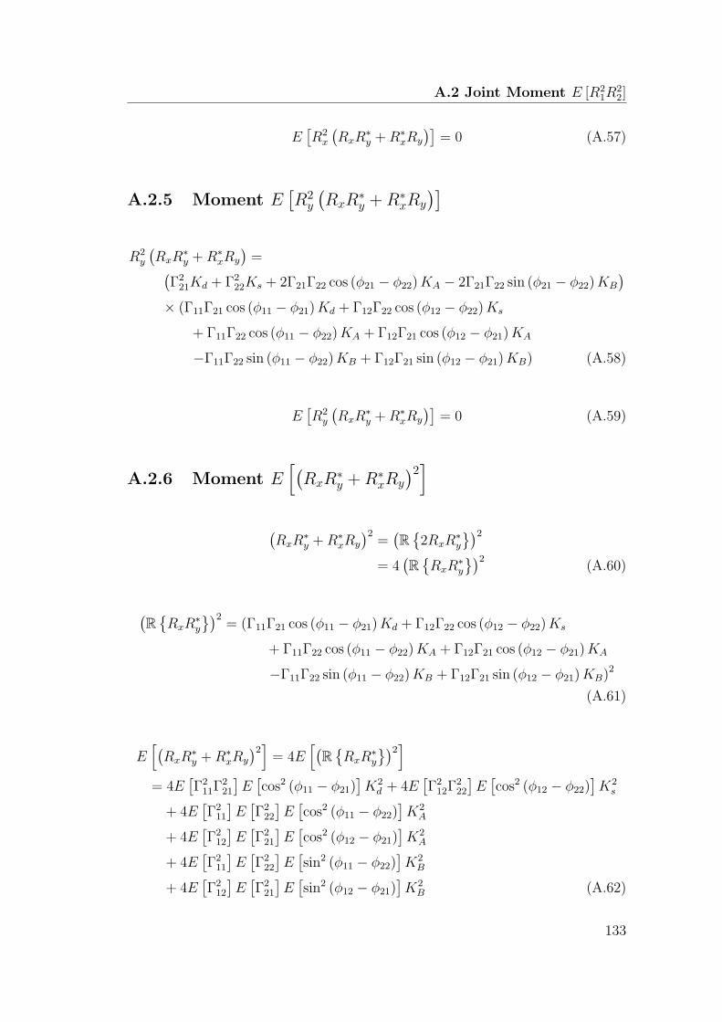
A.2 Joint Moment E [R21R
22]
E[R2
x
(RxR
∗y +R∗
xRy
)]= 0 (A.57)
A.2.5 Moment E[R2y
(RxR
∗y +R∗
xRy
)]R2
y
(RxR
∗y +R∗
xRy
)=(
Γ221Kd + Γ2
22Ks + 2Γ21Γ22 cos (ϕ21 − ϕ22)KA − 2Γ21Γ22 sin (ϕ21 − ϕ22)KB
)× (Γ11Γ21 cos (ϕ11 − ϕ21)Kd + Γ12Γ22 cos (ϕ12 − ϕ22)Ks
+ Γ11Γ22 cos (ϕ11 − ϕ22)KA + Γ12Γ21 cos (ϕ12 − ϕ21)KA
−Γ11Γ22 sin (ϕ11 − ϕ22)KB + Γ12Γ21 sin (ϕ12 − ϕ21)KB) (A.58)
E[R2
y
(RxR
∗y +R∗
xRy
)]= 0 (A.59)
A.2.6 Moment E[(RxR
∗y +R∗
xRy
)2](RxR
∗y +R∗
xRy
)2=(R{2RxR
∗y
})2= 4
(R{RxR
∗y
})2(A.60)
(R{RxR
∗y
})2= (Γ11Γ21 cos (ϕ11 − ϕ21)Kd + Γ12Γ22 cos (ϕ12 − ϕ22)Ks
+ Γ11Γ22 cos (ϕ11 − ϕ22)KA + Γ12Γ21 cos (ϕ12 − ϕ21)KA
−Γ11Γ22 sin (ϕ11 − ϕ22)KB + Γ12Γ21 sin (ϕ12 − ϕ21)KB)2
(A.61)
E[(RxR
∗y +R∗
xRy
)2]= 4E
[(R{RxR
∗y
})2]= 4E
[Γ211Γ
221
]E[cos2 (ϕ11 − ϕ21)
]K2
d + 4E[Γ212Γ
222
]E[cos2 (ϕ12 − ϕ22)
]K2
s
+ 4E[Γ211
]E[Γ222
]E[cos2 (ϕ11 − ϕ22)
]K2
A
+ 4E[Γ212
]E[Γ221
]E[cos2 (ϕ12 − ϕ21)
]K2
A
+ 4E[Γ211
]E[Γ222
]E[sin2 (ϕ11 − ϕ22)
]K2
B
+ 4E[Γ212
]E[Γ221
]E[sin2 (ϕ12 − ϕ21)
]K2
B (A.62)
133

APPENDIX A. Power Correlation Coefficient for the GeneralisedPolarisation Diversity Model
E[(RxR
∗y +R∗
xRy
)2]= 2E
[Γ211Γ
221
]K2
d + 2E[Γ212Γ
222
]K2
s
+ 2(K2
A +K2B
) (E[Γ211
]E[Γ222
]+ E
[Γ212
]E[Γ221
])(A.63)
= 2E[Γ211Γ
221
]K2
d + 2E[Γ212Γ
222
]K2
s
+ 2 (KdKs)(E[Γ211
]E[Γ222
]+ E
[Γ212
]E[Γ221
])(A.64)
A.3 Simplification of E [R1R2]− E [R1]E [R2]
E [R1R2]− E [R1]E [R2]
= sin2 (ψ) cos2 (ψ)E[R4
x
]+ sin4 (ψ)E
[R2
xR2y
]+ cos4 (ψ)E
[R2
xR2y
]+ sin2 (ψ) cos2 (ψ)E
[R4
y
]− sin2 (ψ) cos2 (ψ)E
[(RxR
∗y +R∗
xRy
)2]− sin2 (ψ) cos2 (ψ)E2
[R2
x
]− sin4 (ψ)E
[R2
x
]E[R2
y
]− cos4 (ψ)E
[R2
x
]E[R2
y
]− sin2 (ψ) cos2 (ψ)E2
[R2
y
](A.65)
=1
cos4 (ψ)
(tan2 (ψ)E
[R4
x
]+ tan4 (ψ)E
[R2
xR2y
]+ E
[R2
xR2y
]+ tan2 (ψ)E
[R4
y
]− tan2 (ψ)E
[(RxR
∗y +R∗
xRy
)2]− tan2 (ψ)E2[R2
x
]− tan4 (ψ)E
[R2
x
]E[R2
y
]− E
[R2
x
]E[R2
y
]− tan2 (ψ)E2
[R2
y
])(A.66)
=1
cos4 (ψ)
(2 tan2 (ψ)E2
[R2
x
]+ 2 tan2 (ψ)E2
[R2
y
]− tan2 (ψ)E2
[R2
x
]− tan2 (ψ)E2
[R2
y
]+ tan4 (ψ)K2
dE[Γ211Γ
221
]+ tan4 (ψ)KdKsE
[Γ211
]E[Γ222
]+ tan4 (ψ)KdKsE
[Γ212
]E[Γ221
]+ tan4 (ψ)K2
sE[Γ212Γ
222
]+K2
dE[Γ211Γ
221
]+KdKsE
[Γ211
]E[Γ222
]+KdKsE
[Γ212
]E[Γ221
]+K2
sE[Γ212Γ
222
]− 2 tan2 (ψ)K2
dE[Γ211Γ
221
]− 2 tan2 (ψ)KdKsE
[Γ211
]E[Γ222
]− 2 tan2 (ψ)KdKsE
[Γ212
]E[Γ221
]− 2 tan2 (ψ)K2
sE[Γ212Γ
222
]− tan4 (ψ)E
[R2
x
]E[R2
x
]− E
[R2
x
]E[R2
x
])(A.67)
134

A.4 Moment E [R41]
=1
cos4 (ψ)
(tan2 (ψ)E2
[R2
x
]+ tan2 (ψ)E2
[R2
y
]− 2 tan2 (ψ)E
[R2
x
]E[R2
y
]+ 2 tan2 (ψ)E
[R2
x
]E[R2
y
]− tan4 (ψ)E
[R2
x
]E[R2
y
]− E
[R2
x
]E[R2
y
]+(tan2 (ψ)− 1
)2K2
dE[Γ211Γ
221
]+(tan2 (ψ)− 1
)2KsKdE
[Γ211
]E[Γ222
]+(tan2 (ψ)− 1
)2KsKdE
[Γ212
]E[Γ221
]+(tan2 (ψ)− 1
)2K2
sE[Γ212Γ
222
])(A.68)
E [R1R2]− E [R1]E [R2]
=1
cos4 (ψ)
(tan2 (ψ)
(E[R2
x
]− E
[R2
y
])2+K2
d
(tan2 (ψ)− 1
)2 (E[Γ211Γ
221
]− E
[Γ211
]E[Γ221
])+K2
s
(tan2 (ψ)− 1
)2 (E[Γ212Γ
222
]− E
[Γ212
]E[Γ222
]))(A.69)
=1
cos4 (ψ)
(tan2 (ψ)
(E[R2
x
]− E
[R2
y
])2+ β
(tan2 (ψ)− 1
)2)(A.70)
where
β = K2d
(E[Γ211Γ
221
]− E
[Γ211
]E[Γ221
])+K2
s
(E[Γ212Γ
222
]− E
[Γ212
]E[Γ222
])(A.71)
A.4 Moment E[R4
1
]R4
1 =(R2
x sin2 (ψ) +R2
y cos2 (ψ) + sin (ψ) cos (ψ)
(RxR
∗y +R∗
xRy
))2(A.72)
= R4x sin
4 (ψ) + 2R2xR
2y sin
2 (ψ) cos2 (ψ) + 2 sin3 (ψ) cos (ψ)R2x
(RxR
∗y +R∗
xRy
)+R4
y cos4 (ψ) + 2 sin (ψ) cos3 (ψ)R2
y
(RxR
∗y +R∗
xRy
)+ sin2 (ψ) cos2 (ψ)
(RxR
∗y +R∗
xRy
)2(A.73)
135

APPENDIX A. Power Correlation Coefficient for the GeneralisedPolarisation Diversity Model
E[R4
1
]= sin4 (ψ)E
[R4
x
]+ 2 sin2 (ψ) cos2 (ψ)E
[R2
xR2y
]+ cos4 (ψ)E
[R4
y
]+ sin2 (ψ) cos2 (ψ)E
[(RxR
∗y +R∗
xRy
)2](A.74)
A.5 Moment E[R4
2
]R4
2 =(R2
x cos2 (ψ) +R2
y sin2 (ψ)− sin (ψ) cos (ψ)
(RxR
∗y +R∗
xRy
))2(A.75)
= R4x cos
4 (ψ) + 2R2xR
2y sin
2 (ψ) cos2 (ψ)− 2 sin (ψ) cos3 (ψ)R2x
(RxR
∗y +R∗
xRy
)+R4
y sin4 (ψ)− 2 sin3 (ψ) cos (ψ)R2
y
(RxR
∗y +R∗
xRy
)+ sin2 (ψ) cos2 (ψ)
(RxR
∗y +R∗
xRy
)2(A.76)
E[R4
2
]= cos4 (ψ)E
[R4
x
]+ 2 sin2 (ψ) cos2 (ψ)E
[R2
xR2y
]+ sin4 (ψ)E
[R4
y
]+ sin2 (ψ) cos2 (ψ)E
[(RxR
∗y +R∗
xRy
)2](A.77)
A.6 Simplification of E[R4
1
]− E2
[R2
1
]E[R4
1
]− E2
[R2
1
]= sin4 (ψ)E
[R4
x
]+ 2 sin2 (ψ) cos2 (ψ)E
[R2
xR2y
]+ cos4 (ψ)E
[R4
y
]+ sin2 (ψ) cos2 (ψ)E
[(RxR
∗y +R∗
xRy
)2]− sin4 (ψ)E2[R2
x
]− cos4 (ψ)E2
[R2
y
]− 2 sin2 (ψ) cos2 (ψ)E
[R2
x
]E[R2
y
](A.78)
= 2 sin4 (ψ)E2[R2
x
]+ 2 cos2 (ψ)E2
[R2
y
]− sin4 (ψ)E2
[R2
x
]− cos4 (ψ)E2
[R2
y
]+ 2 sin2 (ψ) cos2 (ψ)
(E[R2
xR2y
]− E
[R2
x
]E[R2
y
])+ sin2 (ψ) cos2 (ψ)E
[(RxR
∗y +R∗
xRy
)2](A.79)
=1
cos4 (ψ)
(tan4 (ψ)E2
[R2
x
]+ 2 tan2 (ψ)E
[R2
x
]E[R2
y
]+ E2
[R2
y
]+4 tan2 (ψ)
(E[R2
xR2y
]− E
[R2
x
]E[R2
y
]))(A.80)
=1
cos4 (ψ)
((tan2 (ψ)E
[R2
x
]+ E
[R2
y
])2+ 4β tan2 (ψ)
)(A.81)
136

A.7 Simplification of E [R42]− E2 [R2
2]
A.7 Simplification of E[R4
2
]− E2
[R2
2
]E[R4
2
]− E2
[R2
2
]= cos4 (ψ)E
[R4
x
]+ 2 sin2 (ψ) cos2 (ψ)E
[R2
xR2y
]+ sin4 (ψ)E
[R4
y
]+ sin2 (ψ) cos2 (ψ)E
[(RxR
∗y +R∗
xRy
)2]− cos4 (ψ)E2[R2
x
]− sin4 (ψ)E2
[R2
y
]− 2 sin2 (ψ) cos2 (ψ)E
[R2
x
]E[R2
y
](A.82)
= 2 cos4 (ψ)E2[R2
x
]+ 2 sin2 (ψ)E2
[R2
y
]− cos4 (ψ)E2
[R2
x
]− sin4 (ψ)E2
[R2
y
]+ 2 sin2 (ψ) cos2 (ψ)
(E[R2
xR2y
]− E
[R2
x
]E[R2
y
])+ sin2 (ψ) cos2 (ψ)E
[(RxR
∗y +R∗
xRy
)2](A.83)
=1
cos4 (ψ)
(E2[R2
x
]+ 2 tan2 (ψ)E
[R2
x
]E[R2
y
]+ tan4 (ψ)E2
[R2
y
]+4 tan2 (ψ)
(E[R2
xR2y
]− E
[R2
x
]E[R2
y
]))(A.84)
=1
cos4 (ψ)
((E[R2
x
]+ tan2 (ψ)E
[R2
y
])2+ 4β tan2 (ψ)
)(A.85)
A.8 Generalised Correlation Coefficient Expres-
sion
The expression of the generalised correlation coefficient is obtained by substitut-
ing the results of Sections A.3, A.6 and A.7 into (A.1).
ρp =E [R2
1R22]− E [R2
1]E [R22]√
(E [R41]− E2 [R2
1]) (E [R42]− E2 [R2
2])(A.86)
ρp =tan2 (ψ)
(E[R2x
]− E
[R2y
])2+ β
(tan2 (ψ)− 1
)2√[(tan2 (ψ)E
[R2
x
]+ E
[R2y
])2+ 4β tan2 (ψ)
] [(E[R2x
]+ tan2 (ψ)E
[R2
y
])2+ 4β tan2 (ψ)
](A.87)
where
β = K2d
(E[Γ211Γ
221
]− E
[Γ211
]E[Γ221
])+K2
s
(E[Γ212Γ
222
]− E
[Γ212
]E[Γ222
])(A.88)
137


References
[1] “Telstra 4G (LTE) on the Next G R⃝network.” [Online]. Available:
http://telstra.com.au/mobile/networks/network info/4g.html
[2] F. Adachi, M. Feeney, J. Parsons, and A. Williamson, “Crosscorrelation
between the envelopes of 900 mhz signals received at a mobile radio base
station site,” Communications, Radar and Signal Processing, IEE Proceed-
ings F, vol. 133, no. 6, pp. 506 – 512, October 1986.
[3] H. Alasti, K. Xu, and Z. Dang, “Efficient experimental path loss exponent
measurement for uniformly attenuated indoor radio channels,” in South-
eastcon, 2009. SOUTHEASTCON ’09. IEEE, March 2009, pp. 255 – 260.
[4] F. Altman and W. Sichak, “A simplified diversity communication system
for beyond-the-horizon links,” Communications Systems, IRE Transactions
on, vol. 4, no. 1, pp. 50 – 55, March 1956.
[5] V. Anreddy and M. Ingram, “Capacity of measured Ricean and Rayleigh in-
door MIMO channels at 2.4 GHz with polarization and spatial diversity,” in
Wireless Communications and Networking Conference, 2006. WCNC 2006.
IEEE, vol. 2, April 2006, pp. 946 – 951.
[6] C. Balanis, Advanced engineering electromagnetics. New York: Wiley,
1989.
[7] S. Bergmann and H. Arnold, “Polarisation diversity in portable communi-
cations environment,” Electronics Letters, vol. 22, no. 11, pp. 609 – 610,
1986.
[8] R. Bernhardt, “Macroscopic diversity in frequency reuse radio systems,”
Selected Areas in Communications, IEEE Journal on, vol. 5, no. 5, pp. 862
– 870, Jun 1987.

REFERENCES
[9] A. Broumandan, J. Nielsen, and G. Lachapelle, “Signal detection perfor-
mance in rayleigh fading environments with a moving antenna,” Signal
Processing, IET, vol. 4, no. 2, pp. 117 – 129, April 2010.
[10] T. W. C. Brown, S. R. Saunders, S. Stavrou, and M. Fiacco, “Characteri-
zation of polarization diversity at the mobile,” Vehicular Technology, IEEE
Transactions on, vol. 56, no. 5, pp. 2440 – 2447, 2007.
[11] A. Buke, M. Hajian, L. Ligthart, and P. Gardner, “Indoor channel measure-
ments using polarisation diversity,” in Vehicular Technology Conference,
1999. VTC 1999 - Fall. IEEE VTS 50th, vol. 4, 1999, pp. 2282 – 2287.
[12] R. Bultitude, “Measured characteristics of 800/900 mhz fading radio chan-
nels with high angle propagation through moderately dense foliage,” Se-
lected Areas in Communications, IEEE Journal on, vol. 5, no. 2, pp. 116 –
127, Feb 1987.
[13] D. Chizhik, J. Ling, and R. Valenzuela, “The effect of electric field polariza-
tion on indoor propagation,” in Universal Personal Communications, 1998.
ICUPC ’98. IEEE 1998 International Conference on, vol. 1, Oct 1998, pp.
459 – 462.
[14] K. Cho, T. Hori, and K. Kagoshima, “Effectiveness of four-branch height
and polarization diversity configuration for street microcell,” Antennas and
Propagation, IEEE Transactions on, vol. 46, no. 6, pp. 776 – 781, Jun 1998.
[15] J. Colburn, Y. Rahmat-Samii, M. Jensen, and G. Pottie, “Evaluation of
personal communications dual-antenna handset diversity performance,” Ve-
hicular Technology, IEEE Transactions on, vol. 47, no. 3, pp. 737 – 746,
Aug 1998.
[16] N. S. Correal and B. D. Woerner, “Enhanced ds-cdma uplink performance
through base station polarization diversity and multistage interference can-
cellation,” in Global Telecommunications Conference, 1998. GLOBECOM
98. The Bridge to Global Integration. IEEE, vol. 4, 1998, pp. 1905 – 1910.
[17] D. Cox, “Antenna diversity performance in mitigating the effects of portable
radiotelephone orientation and multipath propagation,” Communications,
IEEE Transactions on, vol. 31, no. 5, pp. 620 – 628, May 1983.
140

REFERENCES
[18] D. Cox, R. Murray, H. Arnold, A. Norris, and M. Wazowicz, “Cross-
polarization coupling measured for 800 mhz radio transmission in and
around houses and large buildings,” Antennas and Propagation, IEEE
Transactions on, vol. 34, no. 1, pp. 83 – 87, Jan 1986.
[19] ——, “Crosspolarization coupling measured for 800 mhz radio transmis-
sion in and around houses and large buildings,” in Vehicular Technology
Conference, 1985. 35th IEEE, vol. 35, May 1985, pp. 50 – 55.
[20] D. Cox, R. Murray, and A. Norris, “800mhz attenuation measured in and
around suburban houses,” AT&T Bell Laboratory Technical Journal, vol.
673, no. 6, July-August 1984.
[21] I. Cuinas, M. Sanchez, and A. Alejos, “Depolarization due to scattering on
walls in the 5 ghz band,” Antennas and Propagation, IEEE Transactions
on, vol. 57, no. 6, pp. 1804 – 1812, June 2009.
[22] K. Davies and E. Smith, “Ionospheric effects on satellite land mobile sys-
tems,” Antennas and Propagation Magazine, IEEE, vol. 44, no. 6, pp. 24 –
31, Dec 2002.
[23] V. Dehghanian, J. Nielsen, and G. Lachapelle, “Combined spatial-
polarization correlation function for indoor multipath environments,” in
Wireless Communication Systems (ISWCS), 2010 7th International Sym-
posium on, Sept. 2010, pp. 874 – 876.
[24] J. Dietrich, C.B., K. Dietze, J. Nealy, and W. Stutzman, “Spatial, polar-
ization, and pattern diversity for wireless handheld terminals,” Antennas
and Propagation, IEEE Transactions on, vol. 49, no. 9, pp. 1271 – 1281,
Sept 2001.
[25] Y. Ebine and Y. Yamada, “A vehicular-mounted vertical space diversity
antenna for a land mobile radio,” Vehicular Technology, IEEE Transactions
on, vol. 40, no. 2, pp. 420 – 425, May 1991.
[26] P. Eggers, I. Kovacs, and K. Olesen, “Penetration effects on xpd with gsm
1800 handset antennas, relevant for bs polarization diversity for indoor
coverage,” in Vehicular Technology Conference, 1998. VTC 98. 48th IEEE,
vol. 3, May 1998, pp. 1959 – 1963.
141

REFERENCES
[27] P. Eggers, J. Toftgard, and A. Oprea, “Antenna systems for base station di-
versity in urban small and micro cells,” Selected Areas in Communications,
IEEE Journal on, vol. 11, no. 7, pp. 1046 – 1057, Sep 1993.
[28] D. Emmer, E. Humburg, P. Weber, and M. Weckerle, “Measurements of
base station two-branch space and polarization diversity reception and a
comparison of the diversity gain based on the cdf of signal level and simu-
lations of ber in a gsm system,” in Vehicular Technology Conference, 1998.
VTC 98. 48th IEEE, vol. 1, May 1998, pp. 5 – 10.
[29] V. Erceg, L. Greenstein, S. Tjandra, S. Parkoff, A. Gupta, B. Kulic,
A. Julius, and R. Jastrzab, “An empirically-based path loss model for
wireless channels in suburban environments,” in Global Telecommunica-
tions Conference, 1998. GLOBECOM 98. The Bridge to Global Integration.
IEEE, vol. 2, 1998, pp. 922 – 927.
[30] R. B. Ertel and J. H. Reed, “Generation of two equal power correlated
rayleigh fading envelopes,” Communications Letters, IEEE, vol. 2, no. 10,
pp. 276–278, 1998.
[31] M. Feeney and J. Parsons, “Cross-correlation between 900 mhz signals re-
ceived on vertically separated antennas in small-cell mobile radio systems,”
Communications, Speech and Vision, IEE Proceedings I, vol. 138, no. 2, pp.
81 – 86, April 1991.
[32] E. Florman, “Comparison of space-polarization and space-frequency diver-
sities,” Communication Technology, IEEE Transactions on, vol. 16, no. 2,
pp. 283 – 288, April 1968.
[33] K. Fujimori and H. Arai, “Polarization characteristics under indoor mi-
cro/pico cell environments,” Antennas and Propagation, Tenth Interna-
tional Conference on (Conf. Publ. No. 436), vol. 2, pp. 302 – 305, Apr
1997.
[34] A. Fung, “Scattering and depolarization of em waves from a rough surface,”
Proceedings of the IEEE, vol. 54, no. 3, pp. 395 – 396, March 1966.
[35] J. Glaser and L. Faber, “Evaluation of polarization diversity performance,”
Proceedings of the IRE, vol. 41, no. 12, pp. 1774 – 1778, Dec. 1953.
142

REFERENCES
[36] B. Green and M. Jensen, “Diversity performance of personal communica-
tions handset antennas near operator tissue,” in Antennas and Propagation
Society International Symposium, 1997. IEEE., 1997 Digest, vol. 2, Jul
1997, pp. 1182 – 1185.
[37] X. Gui and T. S. Ng, “Performance of asynchronous orthogonal multicar-
rier cdma system in frequency selective fading channel,” Communications,
IEEE Transactions on, vol. 47, no. 7, pp. 1084–1091, 1999, 0090-6778.
[38] M. Hata, “Empirical formula for propagation loss in land mobile radio ser-
vices,” Vehicular Technology, IEEE Transactions on, vol. 29, no. 3, pp. 317
– 325, Aug. 1980.
[39] S. Haykin, Communication Systems. New York ; Chichester: Wiley, 2001.
[40] K. Herring, J. Holloway, D. Staelin, and D. Bliss, “Path-loss characteristics
of urban wireless channels,” Antennas and Propagation, IEEE Transactions
on, vol. 58, no. 1, pp. 171 – 177, Jan. 2010.
[41] S. H. Hong, Y. S. Lee, M. S. Choi, and Y. J. Yoon, “Polarization diversity
with directional antennas for indoor environments,” Microwave Conference,
1999 Asia Pacific, vol. 3, pp. 785 – 788, 1999.
[42] W. C. Jakes, “A comparison of specific space diversity techniques for re-
duction of fast fading in uhf mobile radio systems,” Vehicular Technology,
IEEE Transactions on, vol. 20, no. 4, pp. 81 – 92, 1971.
[43] W. Jakes, Microwave mobile communications, ser. An IEEE Press classic
reissue. IEEE Press, 1994.
[44] J. Jootar, J.-F. Diouris, and J. Zeidler, “Performance of polarization di-
versity in correlated nakagami-m fading channels,” Vehicular Technology,
IEEE Transactions on, vol. 55, no. 1, pp. 128 – 136, Jan. 2006.
[45] R. M. Joyce, D. E. Barker, M. A. McCarthy, and M. T. Feeney, “A study
into the use of polarisation diversity in a dual band 900/1800 mhz gsm net-
work in urban and suburban environments,” in Antennas and Propagation,
1999. IEE National Conference on., 1999, pp. 316 – 319.
143

REFERENCES
[46] J. Karlellopoulos and A. Serras, “Prediction of the rain depolarization
statistics for a microwave radio link,” in Microwave Conference, 1983. 13th
European, Sept. 1983, pp. 615 – 620.
[47] D. Kitchener, J. Dalley, and M. Smith, “Antenna diversity in outdoor mi-
crocells,” Antennas and Propagation, 1995., Ninth International Confer-
ence on (Conf. Publ. No. 407), vol. 2, pp. 1 – 4, Apr 1995.
[48] S. Kozono, T. Tsuruhara, and M. Sakamoto, “Base station polarization
diversity reception for mobile radio,” Vehicular Technology, IEEE Trans-
actions on, vol. 33, no. 4, pp. 301 – 306, Nov 1984.
[49] A. Kucar, “Mobile radio: An overview,” Communications Magazine, IEEE,
vol. 29, no. 11, pp. 72 – 85, Nov 1991.
[50] Y. Kurdi, L. de Haro y Ariel, and M. Sanchez, “Doa for polarization compo-
nents and diversity combination from indoor measurements,” in Antennas
and Propagation Society International Symposium, 2005 IEEE, vol. 4A,
July 2005, pp. 142 – 145.
[51] S.-C. Kwon and G. Stuber, “Cross-polarization discrimination in vehicle-
to-vehicle channels: Geometry-based statistical modeling,” in GLOBECOM
2010, 2010 IEEE Global Telecommunications Conference, Dec. 2010, pp. 1
– 5.
[52] J. Laiho-Steffens, J. Lempiainen, M. Salmenkaita, J. Siltaniemi, and
O. Jukarainen, “Experimental evaluation of polarisation diversity gain at
the base station end in a gsm900 network,” Vehicular Technology Confer-
ence, 1998. VTC 98. 48th IEEE, vol. 1, pp. 16 – 20, May 1998.
[53] J. Laiho-Steffens and J. Lempiainen, “Impact of the mobile antenna incli-
nation on the polarisation diversity gain in a dcs 1800 network,” Personal,
Indoor and Mobile Radio Communications, 1997. ’Waves of the Year 2000’.
PIMRC ’97., The 8th IEEE International Symposium on, vol. 2, pp. 580 –
583, Sep 1997.
[54] W. Lee, “Effects on correlation between two mobile radio base-station an-
tennas,” Communications, IEEE Transactions on, vol. 21, no. 11, pp. 1214
– 1224, Nov 1973.
144

REFERENCES
[55] W. Lee and Y. Yeh, “Polarization diversity system for mobile radio,” Com-
munications, IEEE Transactions on, vol. 20, no. 5, pp. 912 – 923, Oct
1972.
[56] W. Lee, Mobile communications engineering: theory and applications, ser.
McGraw-Hill telecommunications. McGraw-Hill, 1998.
[57] M. LeFevre, M. Jensen, and M. Rice, “Indoor measurement of handset
dual-antenna diversity performance,” in Vehicular Technology Conference,
1997, IEEE 47th, vol. 3, may 1997, pp. 1763 – 1767.
[58] J. F. Lemieux, M. S. El-Tanany, and H. M. Hafez, “Experimental evaluation
of space/frequency/polarization diversity in the indoor wireless channel,”
Vehicular Technology, IEEE Transactions on, vol. 40, no. 3, pp. 569 – 574,
1991.
[59] J. Lempiainen and J. Laiho-Steffens, “The performance of polarization di-
versity schemes at a base station in small/micro cells at 1800 mhz,” Ve-
hicular Technology, IEEE Transactions on, vol. 47, no. 3, pp. 1087 – 1092,
Aug 1998.
[60] J. Lempiainen, J. Laiho-Steffens, and A. Wacker, “Experimental results
of cross polarization discrimination and signal correlation values for a po-
larization diversity scheme,” Vehicular Technology Conference, 1997 IEEE
47th, vol. 3, pp. 1498 – 1502, May 1997.
[61] Y. Liang, J. Zhang, Y. Zhang, and X. Nie, “Investigation of polarization
configurations and the impacts on fading correlation characteristics,” in
Vehicular Technology Conference Fall (VTC 2009-Fall), 2009 IEEE 70th,
Sept. 2009, pp. 1 – 5.
[62] S. Lin, T. Lee, and M. Gardina, “Diversity protections for digital radio-
summary of ten-year experiments and studies,” Communications Magazine,
IEEE, vol. 26, no. 2, pp. 51 – 63, Feb 1988.
[63] F. Lotse, J. E. Berg, U. Forssen, and P. Idahl, “Base station polarization
diversity reception in macrocellular systems at 1800 mhz,” in Vehicular
Technology Conference, 1996. ’Mobile Technology for the Human Race’.,
IEEE 46th, vol. 3, 1996, pp. 1643 – 1646.
145

REFERENCES
[64] L. C. Lukama, D. J. Edwards, and A. Wain, “Application of three-branch
polarisation diversity in the indoor environment,” Communications, IEE
Proceedings-, vol. 150, no. 5, pp. 399 – 403, 2003.
[65] P. Mattheijssen, M. Herben, G. Dolmans, and L. Leyten, “Antenna-pattern
diversity versus space diversity for use at handhelds,” Vehicular Technology,
IEEE Transactions on, vol. 53, no. 4, pp. 1035 – 1042, July 2004.
[66] T. May and H. Rohling, “Reducing the peak-to-average power ratio in ofdm
radio transmission systems,” in Vehicular Technology Conference, 1998.
VTC 98. 48th IEEE, vol. 3, May 1998, pp. 2474 – 2478.
[67] W. McGladdery and S. Stapleton, “Investigation of polarization effects in
indoor radio propagation,” Wireless Communications, 1992. Conference
Proceedings., 1992 IEEE International Conference on Selected Topics in,
pp. 53 – 56, Jun 1992.
[68] M. Nakano, S. Aizawa, T. Satoh, T. Matsuoka, and H. Arai, “Up-link po-
larization diversity measurement for cellular communication systems using
hand-held terminal,” in Antennas and Propagation Society International
Symposium, 1997. IEEE., 1997 Digest, vol. 2, Jul 1997, pp. 1360 – 1363.
[69] R. M. Narayanan, K. Atanassov, V. Stoiljkovic, and G. R. Kadambi, “Po-
larization diversity measurements and analysis for antenna configurations
at 1800 mhz,” Antennas and Propagation, IEEE Transactions on, vol. 52,
no. 7, pp. 1795 – 1810, 2004.
[70] T. Neubauer and P. Eggers, “Simultaneous characterization of polariza-
tion matrix components in pico cells,” in Vehicular Technology Conference,
1999. VTC 1999 - Fall. IEEE VTS 50th, vol. 3, 1999, pp. 1361 – 1365.
[71] S. Oh, S. Kaul, and M. Gruteser, “Exploiting vertical diversity in vehicular
channel environments,” in Personal, Indoor and Mobile Radio Communi-
cations, 2009 IEEE 20th International Symposium on, Sept. 2009, pp. 958
– 962.
[72] J. D. Parsons, The mobile radio propagation channel. New York: Halsted
Press, 1992.
146

REFERENCES
[73] G. Pedersen, S. Widell, and T. Ostervall, “Handheld antenna diversity eval-
uation in a dcs-1800 small cell,” in Personal, Indoor and Mobile Radio
Communications, 1997. ’Waves of the Year 2000’. PIMRC ’97., The 8th
IEEE International Symposium on, vol. 2, Sep 1997, pp. 584 – 588.
[74] P. Peebles, Probability, random variables, and random signal principles, ser.
McGraw-Hill series in electrical and computer engineering. McGraw Hill,
2001.
[75] P. L. Perini and C. L. Holloway, “Angle and space diversity comparisons
in different mobile radio environments,” Antennas and Propagation, IEEE
Transactions on, vol. 46, no. 6, pp. 764 – 775, 1998.
[76] J. Pierce and S. Stein, “Multiple diversity with nonindependent fading,”
Proceedings of the IRE, vol. 48, no. 1, pp. 89 – 104, Jan. 1960.
[77] M. Prasad, “Path loss exponents deduced from vhf amp; uhf measure-
ments over indian subcontinent and model comparison,” Broadcasting,
IEEE Transactions on, vol. 52, no. 3, pp. 290 – 298, Sept. 2006.
[78] R. Prasad, OFDM for wireless communications systems, ser. Artech House
universal personal communications series. Artech House, 2004.
[79] T. Rappaport, Wireless communications: principles and practice, ser. Pren-
tice Hall communications engineering and emerging technologies series.
Prentice Hall PTR, 2002.
[80] A. Ribeiro, C. Castelli, E. Barrientos, and E. Conforti, “Coherence band-
width in a 1.8-ghz urban mobile radio channel,” inMicrowave and Optoelec-
tronics Conference, 2007. IMOC 2007. SBMO/IEEE MTT-S International,
Oct. 2007, pp. 599 – 602.
[81] S. Ruiz-Boque, M. Vilades, and J. Rodriguez, “Performance of two branch
space and polarization diversity at 900 mhz,” in Vehicular Technology Con-
ference, 1997, IEEE 47th, vol. 3, May 1997, pp. 1493 – 1497.
[82] M. Sadiku, Elements of electromagnetics, ser. Oxford series in electrical and
computer engineering. Oxford University Press, 2001.
147

REFERENCES
[83] M. Sanchez and M. Sanchez, “Analysis of polarization diversity at digital
tv indoor receivers,” Broadcasting, IEEE Transactions on, vol. 46, no. 4,
pp. 233 – 239, Dec 2000.
[84] M. Saunders, “Cross polarization at 18 and 30 ghz due to rain,” Antennas
and Propagation, IEEE Transactions on, vol. 19, no. 2, pp. 273 – 277, Mar.
1971.
[85] A. Serra, A. Guraliuc, P. Nepa, G. Manara, I. Khan, and P. Hall, “Dual-
polarisation and dual-pattern planar antenna for diversity in body-centric
communications,” Microwaves, Antennas Propagation, IET, vol. 4, no. 1,
pp. 106 – 112, January 2010.
[86] B. Sklar, Digital Communications: Fundamentals and Applications. Pren-
tice Hall, 1987.
[87] M. Smith and L. Neal, “A comparison of polarisation and space diversity for
indoor propagation at 900 mhz,” in Universal Personal Communications,
1993. Personal Communications: Gateway to the 21st Century. Conference
Record., 2nd International Conference on, vol. 1, Oct 1993, pp. 74 – 78.
[88] T. B. Sorensen, A. O. Nielsen, P. E. Mogensen, M. Tolstrup, and K. Stef-
fensen, “Performance of two-branch polarisation antenna diversity in an
operational gsm network,” in Vehicular Technology Conference, 1998. VTC
98. 48th IEEE, vol. 2, 1998, pp. 741 – 746.
[89] S. Sorooshyari and D. Daut, “Generation of correlated rayleigh fading en-
velopes for accurate performance analysis of diversity systems,” in Personal,
Indoor and Mobile Radio Communications, 2003. PIMRC 2003. 14th IEEE
Proceedings on, vol. 2, sept. 2003, pp. 1800 – 1804 vol.2.
[90] K. Takahashi, “Diversity effect on vhf space communications,” Antennas
and Propagation, IEEE Transactions on, vol. 17, no. 3, pp. 331 – 337, May
1969.
[91] R. E. Taylor, “Satellite tracking simultaneous-lobing monopulse receiving
system with polarization diversity capability,” Aerospace and Electronic
Systems, IEEE Transactions on, vol. AES-3, no. 4, pp. 664 – 680, July
1967.
148

REFERENCES
[92] H. Thomas, G. Siqueira, and R. Cole, “Polarization diversity for urban
millimetric mobile radio communications: comparison of initial propagation
measurement results with prediction,” in Vehicular Technology Conference,
1992, IEEE 42nd, vol. 2, May 1992, pp. 947 – 950.
[93] J. Turkka and M. Renfors, “Path loss measurements for a non-line-of-sight
mobile-to-mobile environment,” in ITS Telecommunications, 2008. ITST
2008. 8th International Conference on, Oct. 2008, pp. 274 – 278.
[94] A. Turkmani, A. Arowojolu, P. Jefford, and C. Kellett, “An experimental
evaluation of the performance of two-branch space and polarization diver-
sity schemes at 1800 mhz,” Vehicular Technology, IEEE Transactions on,
vol. 44, no. 2, pp. 318 – 326, May 1995.
[95] S. VanWambeck and A. Ross, “Performance of diversity receiving systems,”
Proceedings of the IRE, vol. 39, no. 3, pp. 256 – 264, March 1951.
[96] R. G. Vaughan and J. B. Andersen, “Antenna diversity in mobile commu-
nications,” Vehicular Technology, IEEE Transactions on, vol. 36, no. 4, pp.
149 – 172, 1987.
[97] R. Vaughan, “Polarization diversity in mobile communications,” Vehicular
Technology, IEEE Transactions on, vol. 39, no. 3, pp. 177 – 186, Aug 1990.
[98] ——, “Beam spacing for angle diversity,” in Global Telecommunications
Conference, 1998. GLOBECOM 98. The Bridge to Global Integration.
IEEE, vol. 2, 1998, pp. 928 – 933.
[99] U. Wahlberg, S. Widell, and C. Beckman, “The performance of polariza-
tion diversity antennas at 1800 mhz,” in Antennas and Propagation Society
International Symposium, 1997. IEEE., 1997 Digest, vol. 2, Jul 1997, pp.
1368 – 1371.
[100] J. Walfisch and H. Bertoni, “A theoretical model of uhf propagation in
urban environments,” Antennas and Propagation, IEEE Transactions on,
vol. 36, no. 12, pp. 1788 – 1796, Dec. 1988.
[101] J. Webber, M. Beach, B. Allen, and N. Canagarajah, “Performance in-
vestigation of ds-cdma detectors employing a dual polarised antenna,” in
149

REFERENCES
Vehicular Technology Conference, 2001. VTC 2001 Fall. IEEE VTS 54th,
vol. 3, 2001, pp. 1518 – 1522.
[102] L. Yang, S. Cheng, and H. Wang, “Effects of cyclic prefix on ofdm systems
over time-varying channels,” in Personal, Indoor and Mobile Radio Com-
munications, 2005. PIMRC 2005. IEEE 16th International Symposium on,
vol. 2, Sept. 2005, pp. 750 – 753.
[103] L.-L. Yang and L. Hanzo, “Multicarrier ds-cdma: a multiple access scheme
for ubiquitous broadband wireless communications,” Communications Mag-
azine, IEEE, vol. 41, no. 10, pp. 116–124, 2003, 0163-6804.
150